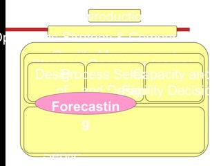
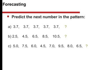
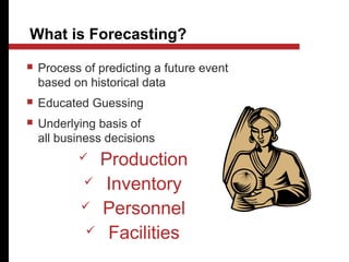
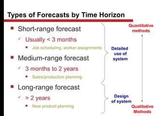
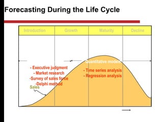
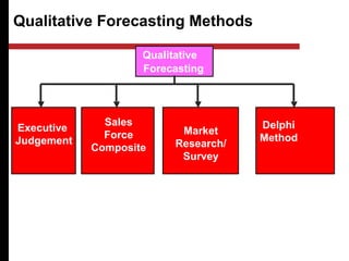
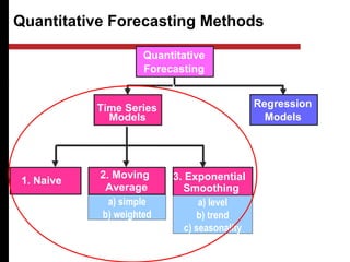
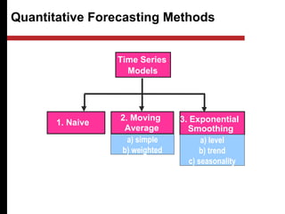
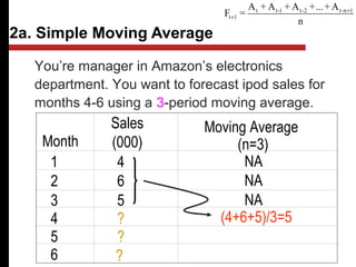
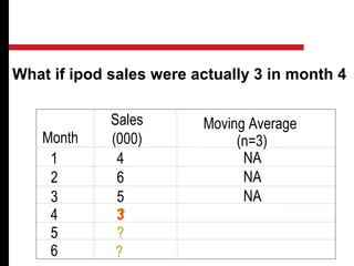
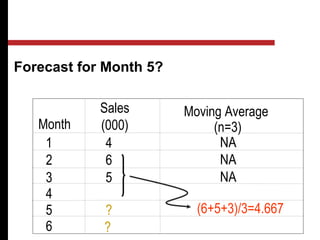
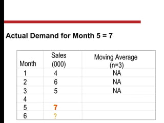
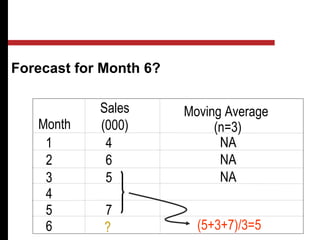
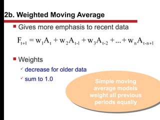
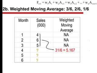
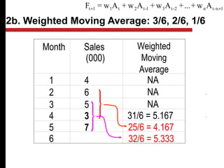
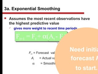
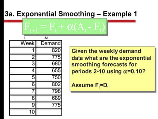
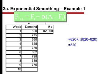
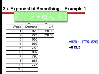
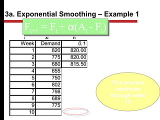
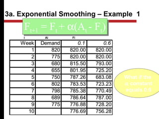
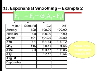
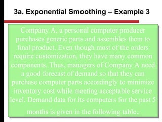
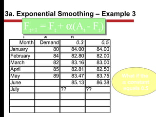
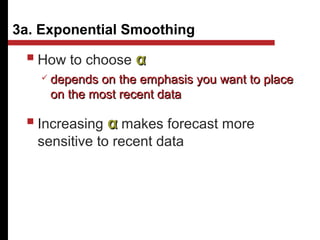
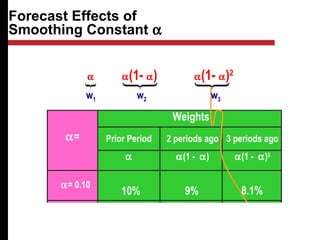
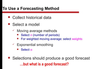
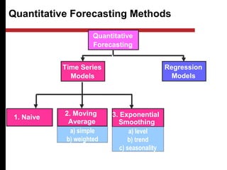
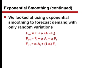
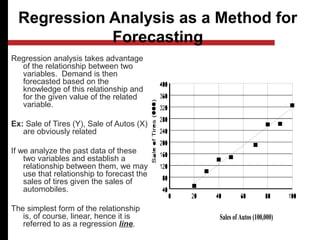
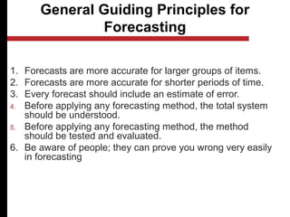
Forecasting
August 29, Wednesday
Introduction
Operations Strategy & Competitivenes
Quality Management
Strategic Decisions (some)
Design
of
Produc
ts
and
Servic
Process Selection
and Design
Capacity and
Facility Decisions
Course
Structure
Forecastin
g
Forecasting
 Predict the next number in the pattern:
a) 3.7, 3.7, 3.7, 3.7, 3.7, ?
b) 2.5, 4.5, 6.5, 8.5, 10.5, ?
c) 5.0, 7.5, 6.0, 4.5, 7.0, 9.5, 8.0, 6.5, ?
Forecasting
 Predict the next number in the pattern:
a) 3.7, 3.7, 3.7, 3.7, 3.7,
b) 2.5, 4.5, 6.5, 8.5, 10.5,
c) 5.0, 7.5, 6.0, 4.5, 7.0, 9.5, 8.0, 6.5,
3.7
12.5
9.0
Outline
 What is forecasting?
 Types of forecasts
 Time-Series forecasting
 Naïve
 Moving Average
 Exponential Smoothing
 Regression
 Good forecasts
What is Forecasting?
 Process of predicting a future event
based on historical data
 Educated Guessing
 Underlying basis of
all business decisions
 Production
 Inventory
 Personnel
 Facilities
In general, forecasts are almost always wrong. So,
Why do we need to forecast?
Throughout the day we forecast very different
things such as weather, traffic, stock market, state
of our company from different perspectives.
Virtually every business attempt is based on
forecasting. Not all of them are derived from
sophisticated methods. However, “Best" educated
guesses about future are more valuable for
purpose of Planning than no forecasts and hence
no planning.
Departments throughout the organization depend on
forecasts to formulate and execute their plans.
Finance needs forecasts to project cash flows and
capital requirements.
Human resources need forecasts to anticipate hiring
needs.
Production needs forecasts to plan production
levels, workforce, material requirements,
inventories, etc.
Importance of Forecasting in OM
Demand is not the only variable of interest to
forecasters.
Manufacturers also forecast worker
absenteeism, machine availability, material
costs, transportation and production lead
times, etc.
Besides demand, service providers are also
interested in forecasts of population, of other
demographic variables, of weather, etc.
Importance of Forecasting in OM
 Short-range forecast
 Usually < 3 months
 Job scheduling, worker assignments
 Medium-range forecast
 3 months to 2 years
 Sales/production planning
 Long-range forecast
 > 2 years
 New product planning
Types of Forecasts by Time Horizon
Design
of system
Detailed
use of
system
Quantitative
methods
Qualitative
Methods
Forecasting During the Life Cycle
Introduction Growth Maturity Decline
Sales
Time
Quantitative models
- Time series analysis
- Regression analysis
Qualitative models
- Executive judgment
- Market research
-Survey of sales force
-Delphi method
Qualitative Forecasting Methods
Qualitative
Forecasting
Models
Market
Research/
Survey
Sales
Force
Composite
Executive
Judgement
Delphi
Method
Smoothing
Briefly, the qualitative methods are:
Executive Judgment: Opinion of a group of high level
experts or managers is pooled
Sales Force Composite: Each regional salesperson
provides his/her sales estimates. Those forecasts are then
reviewed to make sure they are realistic. All regional
forecasts are then pooled at the district and national levels
to obtain an overall forecast.
Market Research/Survey: Solicits input from customers
pertaining to their future purchasing plans. It involves the
use of questionnaires, consumer panels and tests of new
products and services.
Qualitative Methods
Delphi Method: As opposed to regular panels where the individuals
involved are in direct communication, this method eliminates the
effects of group potential dominance of the most vocal members. The
group involves individuals from inside as well as outside the
organization.
Typically, the procedure consists of the following steps:
Each expert in the group makes his/her own forecasts in form of
statements
The coordinator collects all group statements and
summarizes them
The coordinator provides this summary and gives another set
of questions to each
group member including feedback as to the input of other
experts.
The above steps are repeated until a consensus is reached.
.
Qualitative Methods
Quantitative Forecasting Methods
Quantitative
Forecasting
Regression
Models
2. Moving
Average
1. Naive
Time Series
Models
3. Exponential
Smoothing
a) simple
b) weighted
a) level
b) trend
c) seasonality
Quantitative Forecasting Methods
Quantitative
Forecasting
Regression
Models
2. Moving
Average
1. Naive
Time Series
Models
3. Exponential
Smoothing
a) simple
b) weighted
a) level
b) trend
c) seasonality
Time Series Models
 Try to predict the future based on past
data
 Assume that factors influencing the past will
continue to influence the future
RandomRandom
SeasonalSeasonal
TrendTrend
CompositeComposite
Time Series Models: Components
Product Demand over Time
Year
1
Year
2
Year
3
Year
4
Demandforproductorservice
Product Demand over Time
Year
1
Year
2
Year
3
Year
4
Demandforproductorservice
Trend component
Actual
demand line
Seasonal peaks
Random
variation
Now let’s look at some time series approaches to forecasting…
Borrowed from Heizer/Render - Principles of Operations Management, 5e, and Operations Management, 7e
Quantitative Forecasting Methods
Quantitative
Models
2. Moving
Average
1. Naive
Time Series
Models
3. Exponential
Smoothing
a) simple
b) weighted
a) level
b) trend
c) seasonality
1. Naive Approach
 Demand in next period is the same as
demand in most recent period
 May sales = 48 →
 Usually not good
June forecast = 48
2a. Simple Moving Average
n
A+...+A+A+A
=F 1n-t2-t1-tt
1t
+
+
 Assumes an average is a good estimator of
future behavior
 Used if little or no trend
 Used for smoothing
Ft+1 = Forecast for the upcoming period, t+1
n = Number of periods to be averaged
A t = Actual occurrence in period t
2a. Simple Moving Average
You’re manager in Amazon’s electronics
department. You want to forecast ipod sales for
months 4-6 using a 3-period moving average.
n
A+...+A+A+A
=F 1n-t2-t1-tt
1t
+
+
Month
Sales
(000)
1 4
2 6
3 5
4 ?
5 ?
6 ?
2a. Simple Moving Average
Month
Sales
(000)
Moving Average
(n=3)
1 4 NA
2 6 NA
3 5 NA
4 ?
5 ?
(4+6+5)/3=5
6 ?
n
A+...+A+A+A
=F 1n-t2-t1-tt
1t
+
+
You’re manager in Amazon’s electronics
department. You want to forecast ipod sales for
months 4-6 using a 3-period moving average.
What if ipod sales were actually 3 in month 4
Month
Sales
(000)
Moving Average
(n=3)
1 4 NA
2 6 NA
3 5 NA
4 3
5 ?
5
6 ?
2a. Simple Moving Average
?
Forecast for Month 5?
Month
Sales
(000)
Moving Average
(n=3)
1 4 NA
2 6 NA
3 5 NA
4 3
5 ?
5
6 ?
(6+5+3)/3=4.667
2a. Simple Moving Average
Actual Demand for Month 5 = 7
Month
Sales
(000)
Moving Average
(n=3)
1 4 NA
2 6 NA
3 5 NA
4 3
5 7
5
6 ?
4.667
2a. Simple Moving Average
?
Forecast for Month 6?
Month
Sales
(000)
Moving Average
(n=3)
1 4 NA
2 6 NA
3 5 NA
4 3
5 7
5
6 ?
4.667
(5+3+7)/3=5
2a. Simple Moving Average
 Gives more emphasis to recent data
 Weights
 decrease for older data
 sum to 1.0
2b. Weighted Moving Average
1n-tn2-t31-t2t11t Aw+...+Aw+Aw+Aw=F ++
Simple moving
average models
weight all previous
periods equally
Simple moving
average models
weight all previous
periods equally
2b. Weighted Moving Average: 3/6, 2/6, 1/6
Month Weighted
Moving
Average
1 4 NA
2 6 NA
3 5 NA
4 31/6 = 5.167
5
6 ?
?
?
1n-tn2-t31-t2t11t Aw+...+Aw+Aw+Aw=F ++
Sales
(000)
2b. Weighted Moving Average: 3/6, 2/6, 1/6
Month Sales
(000)
Weighted
Moving
Average
1 4 NA
2 6 NA
3 5 NA
4 3 31/6 = 5.167
5 7
6
25/6 = 4.167
32/6 = 5.333
1n-tn2-t31-t2t11t Aw+...+Aw+Aw+Aw=F ++
3a. Exponential Smoothing
 Assumes the most recent observations have
the highest predictive value
 gives more weight to recent time periods
Ft+1 = Ft + α(At - Ft)Ft+1 = Ft + α(At - Ft)
et
Ft+1 = Forecast value for time t+1
At = Actual value at time t
α = Smoothing constant
Need initia
forecast F
to start.
Need initia
forecast F
to start.
3a. Exponential Smoothing – Example 1
Week Demand
1 820
2 775
3 680
4 655
5 750
6 802
7 798
8 689
9 775
10
Given the weekly demand
data what are the exponential
smoothing forecasts for
periods 2-10 using α=0.10?
Assume F1=D1
Given the weekly demand
data what are the exponential
smoothing forecasts for
periods 2-10 using α=0.10?
Assume F1=D1
Ft+1 = Ft + α(At - Ft)Ft+1 = Ft + α(At - Ft)
i Ai
Week Demand 0.1 0.6
1 820 820.00 820.00
2 775 820.00 820.00
3 680 815.50 793.00
4 655 801.95 725.20
5 750 787.26 683.08
6 802 783.53 723.23
7 798 785.38 770.49
8 689 786.64 787.00
9 775 776.88 728.20
10 776.69 756.28
Ft+1 = Ft + α(At - Ft)Ft+1 = Ft + α(At - Ft)
3a. Exponential Smoothing – Example 1
α =
F2 = F1+ α(A1–F1) =820+.1(820–820)
=820
i Ai Fi
Week Demand 0.1 0.6
1 820 820.00 820.00
2 775 820.00 820.00
3 680 815.50 793.00
4 655 801.95 725.20
5 750 787.26 683.08
6 802 783.53 723.23
7 798 785.38 770.49
8 689 786.64 787.00
9 775 776.88 728.20
10 776.69 756.28
Ft+1 = Ft + α(At - Ft)Ft+1 = Ft + α(At - Ft)
3a. Exponential Smoothing – Example 1
α =
F3 = F2+ α(A2–F2) =820+.1(775–820)
=815.5
i Ai Fi
Week Demand 0.1 0.6
1 820 820.00 820.00
2 775 820.00 820.00
3 680 815.50 793.00
4 655 801.95 725.20
5 750 787.26 683.08
6 802 783.53 723.23
7 798 785.38 770.49
8 689 786.64 787.00
9 775 776.88 728.20
10 776.69 756.28
Ft+1 = Ft + α(At - Ft)Ft+1 = Ft + α(At - Ft)
This process
continues
through week
10
3a. Exponential Smoothing – Example 1
α =
i Ai Fi
Week Demand 0.1 0.6
1 820 820.00 820.00
2 775 820.00 820.00
3 680 815.50 793.00
4 655 801.95 725.20
5 750 787.26 683.08
6 802 783.53 723.23
7 798 785.38 770.49
8 689 786.64 787.00
9 775 776.88 728.20
10 776.69 756.28
Ft+1 = Ft + α(At - Ft)Ft+1 = Ft + α(At - Ft)
What if the
α constant
equals 0.6
3a. Exponential Smoothing – Example 1
α = α =
i Ai Fi
Month Demand 0.3 0.6
January 120 100.00 100.00
February 90 106.00 112.00
March 101 101.20 98.80
April 91 101.14 100.12
May 115 98.10 94.65
June 83 103.17 106.86
July 97.12 92.54
August
September
Ft+1 = Ft + α(At - Ft)Ft+1 = Ft + α(At - Ft)
What if the
α constant
equals 0.6
3a. Exponential Smoothing – Example 2
α = α =
i Ai Fi
Company A, a personal computer producer
purchases generic parts and assembles them to
final product. Even though most of the orders
require customization, they have many common
components. Thus, managers of Company A need
a good forecast of demand so that they can
purchase computer parts accordingly to minimize
inventory cost while meeting acceptable service
level. Demand data for its computers for the past 5
months is given in the following table.
3a. Exponential Smoothing – Example 3
Month Demand 0.3 0.5
January 80 84.00 84.00
February 84 82.80 82.00
March 82 83.16 83.00
April 85 82.81 82.50
May 89 83.47 83.75
June 85.13 86.38
July ?? ??
Ft+1 = Ft + α(At - Ft)Ft+1 = Ft + α(At - Ft)
What if the
α constant
equals 0.5
3a. Exponential Smoothing – Example 3
α = α =
i Ai Fi
 How to choose αα
 depends on the emphasis you want to placedepends on the emphasis you want to place
on the most recent dataon the most recent data
 Increasing αα makes forecast more
sensitive to recent data
3a. Exponential Smoothing
Ft+1 = α At + α(1- α) At - 1 + α(1- α)2
At - 2 + ...
Forecast Effects of
Smoothing Constant α
Weights
Prior Period
α
2 periods ago
α(1 - α)
3 periods ago
α(1 - α)2
α=
α= 0.10
α= 0.90
10% 9% 8.1%
90% 9% 0.9%
Ft+1 = Ft + α (At - Ft)
or
w1 w2 w3
 Collect historical data
 Select a model
 Moving average methods
 Select n (number of periods)
 For weighted moving average: select weights
 Exponential smoothing
 Select α
 Selections should produce a good forecast
To Use a Forecasting Method
…but what is a good forecast?
A Good Forecast
♦Has a small error
♦ Error = Demand - Forecast
Measures of Forecast Error
b. MSE = Mean Squared Error ( )
n
F-A
=MSE
n
1=t
2
tt∑
MAD =
A - F
n
t t
t=1
n
∑
et
 Ideal values =0 (i.e., no forecasting error)
MSE=RMSEc. RMSE = Root Mean Squared Error
a. MAD = Mean Absolute Deviation
MAD Example
Month Sales Forecast
1 220 n/a
2 250 255
3 210 205
4 300 320
5 325 315
What is the MAD value given the
forecast values in the table below?
What is the MAD value given the
forecast values in the table below?
MAD =
A - F
n
t t
t=1
n
∑
5
5
20
10
|At – Ft|
FtAt
= 40
= 40
4
=10
MSE/RMSE Example
Month Sales Forecast
1 220 n/a
2 250 255
3 210 205
4 300 320
5 325 315
What is the MSE value?What is the MSE value?
5
5
20
10
|At – Ft|
FtAt
= 550
4
=137.5
(At – Ft)2
25
25
400
100
= 550
( )
n
F-A
=MSE
n
1=t
2
tt∑
RMSE = √137.5
=11.73
Measures of Error
t At
Ft
et
|et
| et
2
Jan 120 100 20 20 400
Feb 90 106 256
Mar 101 102
April 91 101
May 115 98
June 83 103
1. Mean
Absolute
Deviation
(MAD)n
e
MAD
n
t∑
= 12a. Mean
Squared
Error
(MSE)
( )
MSE
e
n
t
n
=
∑
2
1
2b. Root
Mean
Squared
Error
(RMSE)
RMSE MSE=
-16 16
-1 1
-10
17
-20
10
17
20
1
100
289
400
-10 84 1,446
84
6
= 14
1,446
6
= 241
= SQRT(241)
=15.52
An accurate forecasting system will have small MAD,
MSE and RMSE; ideally equal to zero. A large error may
indicate that either the forecasting method used or the
parameters such as αused in the method are wrong.
deviationabsoluteMean
)(
=
MAD
RSFE
=TS
∑ −
t
tt forecastactual
30
 How can we tell if a forecast has a positive or
negative bias?
 TS = Tracking Signal
 Good tracking signal has low values
Forecast Bias
MAD
Quantitative Forecasting Methods
Quantitative
Forecasting
Regression
Models
2. Moving
Average
1. Naive
Time Series
Models
3. Exponential
Smoothing
a) simple
b) weighted
a) level
b) trend
c) seasonality
 We looked at using exponential
smoothing to forecast demand with
only random variations
Exponential Smoothing (continued)
Ft+1 = Ft + α (At - Ft)
Ft+1 = Ft + α At – α Ft
Ft+1 = α At + (1-α) Ft
Exponential Smoothing (continued)
 We looked at using exponential
smoothing to forecast demand with
only random variations
 What if demand varies due to
randomness and trend?
 What if we have trend and seasonality
in the data?
Regression Analysis as a Method for
Forecasting
Regression analysis takes advantage
of the relationship between two
variables. Demand is then
forecasted based on the
knowledge of this relationship and
for the given value of the related
variable.
Ex: Sale of Tires (Y), Sale of Autos (X)
are obviously related
If we analyze the past data of these
two variables and establish a
relationship between them, we may
use that relationship to forecast the
sales of tires given the sales of
automobiles.
The simplest form of the relationship
is, of course, linear, hence it is
referred to as a regression line.
Sales of Autos (100,000)
Formulas
xbya −=
∑
∑
−
−
= 22
xnx
yxnxy
b
x
y
=x
=y
y = a + b x
where,
MonthAdvertising Sales X 2
XY
January 3 1 9.00 3.00
February 4 2 16.00 8.00
March 2 1 4.00 2.00
April 5 3 25.00 15.00
May 4 2 16.00 8.00
June 2 1 4.00 2.00
July
TOTAL 20 10 74 38
y = a + b Xy = a + b X
Regression – Example
∑
∑
−
−
= 22
xnx
yxnxy
b xbya −=
General Guiding Principles for
Forecasting
1. Forecasts are more accurate for larger groups of items.
2. Forecasts are more accurate for shorter periods of time.
3. Every forecast should include an estimate of error.
4. Before applying any forecasting method, the total system
should be understood.
5. Before applying any forecasting method, the method
should be tested and evaluated.
6. Be aware of people; they can prove you wrong very easily
in forecasting
FOR JULY 2nd
MONDAY
 READ THE CHAPTERS ON
 Forecasting
 Product and service design

Forecasting

  • 1.
  • 2.
    Introduction Operations Strategy &Competitivenes Quality Management Strategic Decisions (some) Design of Produc ts and Servic Process Selection and Design Capacity and Facility Decisions Course Structure Forecastin g
  • 3.
    Forecasting  Predict thenext number in the pattern: a) 3.7, 3.7, 3.7, 3.7, 3.7, ? b) 2.5, 4.5, 6.5, 8.5, 10.5, ? c) 5.0, 7.5, 6.0, 4.5, 7.0, 9.5, 8.0, 6.5, ?
  • 4.
    Forecasting  Predict thenext number in the pattern: a) 3.7, 3.7, 3.7, 3.7, 3.7, b) 2.5, 4.5, 6.5, 8.5, 10.5, c) 5.0, 7.5, 6.0, 4.5, 7.0, 9.5, 8.0, 6.5, 3.7 12.5 9.0
  • 5.
    Outline  What isforecasting?  Types of forecasts  Time-Series forecasting  Naïve  Moving Average  Exponential Smoothing  Regression  Good forecasts
  • 6.
    What is Forecasting? Process of predicting a future event based on historical data  Educated Guessing  Underlying basis of all business decisions  Production  Inventory  Personnel  Facilities
  • 7.
    In general, forecastsare almost always wrong. So, Why do we need to forecast? Throughout the day we forecast very different things such as weather, traffic, stock market, state of our company from different perspectives. Virtually every business attempt is based on forecasting. Not all of them are derived from sophisticated methods. However, “Best" educated guesses about future are more valuable for purpose of Planning than no forecasts and hence no planning.
  • 8.
    Departments throughout theorganization depend on forecasts to formulate and execute their plans. Finance needs forecasts to project cash flows and capital requirements. Human resources need forecasts to anticipate hiring needs. Production needs forecasts to plan production levels, workforce, material requirements, inventories, etc. Importance of Forecasting in OM
  • 9.
    Demand is notthe only variable of interest to forecasters. Manufacturers also forecast worker absenteeism, machine availability, material costs, transportation and production lead times, etc. Besides demand, service providers are also interested in forecasts of population, of other demographic variables, of weather, etc. Importance of Forecasting in OM
  • 10.
     Short-range forecast Usually < 3 months  Job scheduling, worker assignments  Medium-range forecast  3 months to 2 years  Sales/production planning  Long-range forecast  > 2 years  New product planning Types of Forecasts by Time Horizon Design of system Detailed use of system Quantitative methods Qualitative Methods
  • 11.
    Forecasting During theLife Cycle Introduction Growth Maturity Decline Sales Time Quantitative models - Time series analysis - Regression analysis Qualitative models - Executive judgment - Market research -Survey of sales force -Delphi method
  • 12.
  • 13.
    Briefly, the qualitativemethods are: Executive Judgment: Opinion of a group of high level experts or managers is pooled Sales Force Composite: Each regional salesperson provides his/her sales estimates. Those forecasts are then reviewed to make sure they are realistic. All regional forecasts are then pooled at the district and national levels to obtain an overall forecast. Market Research/Survey: Solicits input from customers pertaining to their future purchasing plans. It involves the use of questionnaires, consumer panels and tests of new products and services. Qualitative Methods
  • 14.
    Delphi Method: Asopposed to regular panels where the individuals involved are in direct communication, this method eliminates the effects of group potential dominance of the most vocal members. The group involves individuals from inside as well as outside the organization. Typically, the procedure consists of the following steps: Each expert in the group makes his/her own forecasts in form of statements The coordinator collects all group statements and summarizes them The coordinator provides this summary and gives another set of questions to each group member including feedback as to the input of other experts. The above steps are repeated until a consensus is reached. . Qualitative Methods
  • 15.
    Quantitative Forecasting Methods Quantitative Forecasting Regression Models 2.Moving Average 1. Naive Time Series Models 3. Exponential Smoothing a) simple b) weighted a) level b) trend c) seasonality
  • 16.
    Quantitative Forecasting Methods Quantitative Forecasting Regression Models 2.Moving Average 1. Naive Time Series Models 3. Exponential Smoothing a) simple b) weighted a) level b) trend c) seasonality
  • 17.
    Time Series Models Try to predict the future based on past data  Assume that factors influencing the past will continue to influence the future
  • 18.
  • 19.
    Product Demand overTime Year 1 Year 2 Year 3 Year 4 Demandforproductorservice
  • 20.
    Product Demand overTime Year 1 Year 2 Year 3 Year 4 Demandforproductorservice Trend component Actual demand line Seasonal peaks Random variation Now let’s look at some time series approaches to forecasting… Borrowed from Heizer/Render - Principles of Operations Management, 5e, and Operations Management, 7e
  • 21.
    Quantitative Forecasting Methods Quantitative Models 2.Moving Average 1. Naive Time Series Models 3. Exponential Smoothing a) simple b) weighted a) level b) trend c) seasonality
  • 22.
    1. Naive Approach Demand in next period is the same as demand in most recent period  May sales = 48 →  Usually not good June forecast = 48
  • 23.
    2a. Simple MovingAverage n A+...+A+A+A =F 1n-t2-t1-tt 1t + +  Assumes an average is a good estimator of future behavior  Used if little or no trend  Used for smoothing Ft+1 = Forecast for the upcoming period, t+1 n = Number of periods to be averaged A t = Actual occurrence in period t
  • 24.
    2a. Simple MovingAverage You’re manager in Amazon’s electronics department. You want to forecast ipod sales for months 4-6 using a 3-period moving average. n A+...+A+A+A =F 1n-t2-t1-tt 1t + + Month Sales (000) 1 4 2 6 3 5 4 ? 5 ? 6 ?
  • 25.
    2a. Simple MovingAverage Month Sales (000) Moving Average (n=3) 1 4 NA 2 6 NA 3 5 NA 4 ? 5 ? (4+6+5)/3=5 6 ? n A+...+A+A+A =F 1n-t2-t1-tt 1t + + You’re manager in Amazon’s electronics department. You want to forecast ipod sales for months 4-6 using a 3-period moving average.
  • 26.
    What if ipodsales were actually 3 in month 4 Month Sales (000) Moving Average (n=3) 1 4 NA 2 6 NA 3 5 NA 4 3 5 ? 5 6 ? 2a. Simple Moving Average ?
  • 27.
    Forecast for Month5? Month Sales (000) Moving Average (n=3) 1 4 NA 2 6 NA 3 5 NA 4 3 5 ? 5 6 ? (6+5+3)/3=4.667 2a. Simple Moving Average
  • 28.
    Actual Demand forMonth 5 = 7 Month Sales (000) Moving Average (n=3) 1 4 NA 2 6 NA 3 5 NA 4 3 5 7 5 6 ? 4.667 2a. Simple Moving Average ?
  • 29.
    Forecast for Month6? Month Sales (000) Moving Average (n=3) 1 4 NA 2 6 NA 3 5 NA 4 3 5 7 5 6 ? 4.667 (5+3+7)/3=5 2a. Simple Moving Average
  • 30.
     Gives moreemphasis to recent data  Weights  decrease for older data  sum to 1.0 2b. Weighted Moving Average 1n-tn2-t31-t2t11t Aw+...+Aw+Aw+Aw=F ++ Simple moving average models weight all previous periods equally Simple moving average models weight all previous periods equally
  • 31.
    2b. Weighted MovingAverage: 3/6, 2/6, 1/6 Month Weighted Moving Average 1 4 NA 2 6 NA 3 5 NA 4 31/6 = 5.167 5 6 ? ? ? 1n-tn2-t31-t2t11t Aw+...+Aw+Aw+Aw=F ++ Sales (000)
  • 32.
    2b. Weighted MovingAverage: 3/6, 2/6, 1/6 Month Sales (000) Weighted Moving Average 1 4 NA 2 6 NA 3 5 NA 4 3 31/6 = 5.167 5 7 6 25/6 = 4.167 32/6 = 5.333 1n-tn2-t31-t2t11t Aw+...+Aw+Aw+Aw=F ++
  • 33.
    3a. Exponential Smoothing Assumes the most recent observations have the highest predictive value  gives more weight to recent time periods Ft+1 = Ft + α(At - Ft)Ft+1 = Ft + α(At - Ft) et Ft+1 = Forecast value for time t+1 At = Actual value at time t α = Smoothing constant Need initia forecast F to start. Need initia forecast F to start.
  • 34.
    3a. Exponential Smoothing– Example 1 Week Demand 1 820 2 775 3 680 4 655 5 750 6 802 7 798 8 689 9 775 10 Given the weekly demand data what are the exponential smoothing forecasts for periods 2-10 using α=0.10? Assume F1=D1 Given the weekly demand data what are the exponential smoothing forecasts for periods 2-10 using α=0.10? Assume F1=D1 Ft+1 = Ft + α(At - Ft)Ft+1 = Ft + α(At - Ft) i Ai
  • 35.
    Week Demand 0.10.6 1 820 820.00 820.00 2 775 820.00 820.00 3 680 815.50 793.00 4 655 801.95 725.20 5 750 787.26 683.08 6 802 783.53 723.23 7 798 785.38 770.49 8 689 786.64 787.00 9 775 776.88 728.20 10 776.69 756.28 Ft+1 = Ft + α(At - Ft)Ft+1 = Ft + α(At - Ft) 3a. Exponential Smoothing – Example 1 α = F2 = F1+ α(A1–F1) =820+.1(820–820) =820 i Ai Fi
  • 36.
    Week Demand 0.10.6 1 820 820.00 820.00 2 775 820.00 820.00 3 680 815.50 793.00 4 655 801.95 725.20 5 750 787.26 683.08 6 802 783.53 723.23 7 798 785.38 770.49 8 689 786.64 787.00 9 775 776.88 728.20 10 776.69 756.28 Ft+1 = Ft + α(At - Ft)Ft+1 = Ft + α(At - Ft) 3a. Exponential Smoothing – Example 1 α = F3 = F2+ α(A2–F2) =820+.1(775–820) =815.5 i Ai Fi
  • 37.
    Week Demand 0.10.6 1 820 820.00 820.00 2 775 820.00 820.00 3 680 815.50 793.00 4 655 801.95 725.20 5 750 787.26 683.08 6 802 783.53 723.23 7 798 785.38 770.49 8 689 786.64 787.00 9 775 776.88 728.20 10 776.69 756.28 Ft+1 = Ft + α(At - Ft)Ft+1 = Ft + α(At - Ft) This process continues through week 10 3a. Exponential Smoothing – Example 1 α = i Ai Fi
  • 38.
    Week Demand 0.10.6 1 820 820.00 820.00 2 775 820.00 820.00 3 680 815.50 793.00 4 655 801.95 725.20 5 750 787.26 683.08 6 802 783.53 723.23 7 798 785.38 770.49 8 689 786.64 787.00 9 775 776.88 728.20 10 776.69 756.28 Ft+1 = Ft + α(At - Ft)Ft+1 = Ft + α(At - Ft) What if the α constant equals 0.6 3a. Exponential Smoothing – Example 1 α = α = i Ai Fi
  • 39.
    Month Demand 0.30.6 January 120 100.00 100.00 February 90 106.00 112.00 March 101 101.20 98.80 April 91 101.14 100.12 May 115 98.10 94.65 June 83 103.17 106.86 July 97.12 92.54 August September Ft+1 = Ft + α(At - Ft)Ft+1 = Ft + α(At - Ft) What if the α constant equals 0.6 3a. Exponential Smoothing – Example 2 α = α = i Ai Fi
  • 40.
    Company A, apersonal computer producer purchases generic parts and assembles them to final product. Even though most of the orders require customization, they have many common components. Thus, managers of Company A need a good forecast of demand so that they can purchase computer parts accordingly to minimize inventory cost while meeting acceptable service level. Demand data for its computers for the past 5 months is given in the following table. Company A, a personal computer producer purchases generic parts and assembles them to final product. Even though most of the orders require customization, they have many common components. Thus, managers of Company A need a good forecast of demand so that they can purchase computer parts accordingly to minimize inventory cost while meeting acceptable service level. Demand data for its computers for the past 5 months is given in the following table. 3a. Exponential Smoothing – Example 3
  • 41.
    Month Demand 0.30.5 January 80 84.00 84.00 February 84 82.80 82.00 March 82 83.16 83.00 April 85 82.81 82.50 May 89 83.47 83.75 June 85.13 86.38 July ?? ?? Ft+1 = Ft + α(At - Ft)Ft+1 = Ft + α(At - Ft) What if the α constant equals 0.5 3a. Exponential Smoothing – Example 3 α = α = i Ai Fi
  • 42.
     How tochoose αα  depends on the emphasis you want to placedepends on the emphasis you want to place on the most recent dataon the most recent data  Increasing αα makes forecast more sensitive to recent data 3a. Exponential Smoothing
  • 43.
    Ft+1 = αAt + α(1- α) At - 1 + α(1- α)2 At - 2 + ... Forecast Effects of Smoothing Constant α Weights Prior Period α 2 periods ago α(1 - α) 3 periods ago α(1 - α)2 α= α= 0.10 α= 0.90 10% 9% 8.1% 90% 9% 0.9% Ft+1 = Ft + α (At - Ft) or w1 w2 w3
  • 44.
     Collect historicaldata  Select a model  Moving average methods  Select n (number of periods)  For weighted moving average: select weights  Exponential smoothing  Select α  Selections should produce a good forecast To Use a Forecasting Method …but what is a good forecast?
  • 45.
    A Good Forecast ♦Hasa small error ♦ Error = Demand - Forecast
  • 46.
    Measures of ForecastError b. MSE = Mean Squared Error ( ) n F-A =MSE n 1=t 2 tt∑ MAD = A - F n t t t=1 n ∑ et  Ideal values =0 (i.e., no forecasting error) MSE=RMSEc. RMSE = Root Mean Squared Error a. MAD = Mean Absolute Deviation
  • 47.
    MAD Example Month SalesForecast 1 220 n/a 2 250 255 3 210 205 4 300 320 5 325 315 What is the MAD value given the forecast values in the table below? What is the MAD value given the forecast values in the table below? MAD = A - F n t t t=1 n ∑ 5 5 20 10 |At – Ft| FtAt = 40 = 40 4 =10
  • 48.
    MSE/RMSE Example Month SalesForecast 1 220 n/a 2 250 255 3 210 205 4 300 320 5 325 315 What is the MSE value?What is the MSE value? 5 5 20 10 |At – Ft| FtAt = 550 4 =137.5 (At – Ft)2 25 25 400 100 = 550 ( ) n F-A =MSE n 1=t 2 tt∑ RMSE = √137.5 =11.73
  • 49.
    Measures of Error tAt Ft et |et | et 2 Jan 120 100 20 20 400 Feb 90 106 256 Mar 101 102 April 91 101 May 115 98 June 83 103 1. Mean Absolute Deviation (MAD)n e MAD n t∑ = 12a. Mean Squared Error (MSE) ( ) MSE e n t n = ∑ 2 1 2b. Root Mean Squared Error (RMSE) RMSE MSE= -16 16 -1 1 -10 17 -20 10 17 20 1 100 289 400 -10 84 1,446 84 6 = 14 1,446 6 = 241 = SQRT(241) =15.52 An accurate forecasting system will have small MAD, MSE and RMSE; ideally equal to zero. A large error may indicate that either the forecasting method used or the parameters such as αused in the method are wrong.
  • 50.
    deviationabsoluteMean )( = MAD RSFE =TS ∑ − t tt forecastactual 30 How can we tell if a forecast has a positive or negative bias?  TS = Tracking Signal  Good tracking signal has low values Forecast Bias MAD
  • 51.
    Quantitative Forecasting Methods Quantitative Forecasting Regression Models 2.Moving Average 1. Naive Time Series Models 3. Exponential Smoothing a) simple b) weighted a) level b) trend c) seasonality
  • 52.
     We lookedat using exponential smoothing to forecast demand with only random variations Exponential Smoothing (continued) Ft+1 = Ft + α (At - Ft) Ft+1 = Ft + α At – α Ft Ft+1 = α At + (1-α) Ft
  • 53.
    Exponential Smoothing (continued) We looked at using exponential smoothing to forecast demand with only random variations  What if demand varies due to randomness and trend?  What if we have trend and seasonality in the data?
  • 54.
    Regression Analysis asa Method for Forecasting Regression analysis takes advantage of the relationship between two variables. Demand is then forecasted based on the knowledge of this relationship and for the given value of the related variable. Ex: Sale of Tires (Y), Sale of Autos (X) are obviously related If we analyze the past data of these two variables and establish a relationship between them, we may use that relationship to forecast the sales of tires given the sales of automobiles. The simplest form of the relationship is, of course, linear, hence it is referred to as a regression line. Sales of Autos (100,000)
  • 55.
  • 56.
    MonthAdvertising Sales X2 XY January 3 1 9.00 3.00 February 4 2 16.00 8.00 March 2 1 4.00 2.00 April 5 3 25.00 15.00 May 4 2 16.00 8.00 June 2 1 4.00 2.00 July TOTAL 20 10 74 38 y = a + b Xy = a + b X Regression – Example ∑ ∑ − − = 22 xnx yxnxy b xbya −=
  • 57.
    General Guiding Principlesfor Forecasting 1. Forecasts are more accurate for larger groups of items. 2. Forecasts are more accurate for shorter periods of time. 3. Every forecast should include an estimate of error. 4. Before applying any forecasting method, the total system should be understood. 5. Before applying any forecasting method, the method should be tested and evaluated. 6. Be aware of people; they can prove you wrong very easily in forecasting
  • 58.
    FOR JULY 2nd MONDAY READ THE CHAPTERS ON  Forecasting  Product and service design

Editor's Notes

  • #11 At this point, it may be useful to point out the “time horizons” considered by different industries. For example, some colleges and universities look 30 to fifty years ahead, industries engaged in long distance transportation (steam ship, railroad) or provision of basic power (electrical and gas utilities, etc.) also look far ahead (20 to 100 years). Ask them to give examples of industries having much shorter long-range horizons.
  • #13 A point you may wish to make here is that only in the case of linear regression are we assuming that we know “why” something happened. General time-series models are based exclusively on “what” happened in the past; not at all on “why.” Does operating in a time of drastic change imply limitations on our ability to use time series models?
  • #16 A point you may wish to make here is that only in the case of linear regression are we assuming that we know “why” something happened. General time-series models are based exclusively on “what” happened in the past; not at all on “why.” Does operating in a time of drastic change imply limitations on our ability to use time series models?
  • #17 A point you may wish to make here is that only in the case of linear regression are we assuming that we know “why” something happened. General time-series models are based exclusively on “what” happened in the past; not at all on “why.” Does operating in a time of drastic change imply limitations on our ability to use time series models?
  • #20 This slide illustrates a typical demand curve. You might ask students why it is important to know more than simply the actual demand over time. Why, for example, would one wish to be able to break out a “seasonality” factor?
  • #21 This slide illustrates a typical demand curve. You might ask students why it is important to know more than simply the actual demand over time. Why, for example, would one wish to be able to break out a “seasonality” factor?
  • #22 A point you may wish to make here is that only in the case of linear regression are we assuming that we know “why” something happened. General time-series models are based exclusively on “what” happened in the past; not at all on “why.” Does operating in a time of drastic change imply limitations on our ability to use time series models?
  • #23 This slide introduces the naïve approach. Subsequent slides introduce other methodologies.
  • #31 This slide introduces the “weighted moving average” method. It is probably most important to discuss choice of the weights.
  • #43 These points should have been brought out in the example, but can be summarized here.
  • #44 This slide illustrates the decrease in magnitude of the smoothing constant. In the Power Point presentation, the several previous slides show the steps leading to this slide.
  • #45 This slide introduces the exponential smoothing method of time series forecasting. The following slide contains the equations, and an example follows.
  • #46 This slide indicates one method of selecting .
  • #47 This slide illustrates the equations for two measures of forecast error. Students might be asked if there is an occasion when one method might be preferred over the other.
  • #52 A point you may wish to make here is that only in the case of linear regression are we assuming that we know “why” something happened. General time-series models are based exclusively on “what” happened in the past; not at all on “why.” Does operating in a time of drastic change imply limitations on our ability to use time series models?