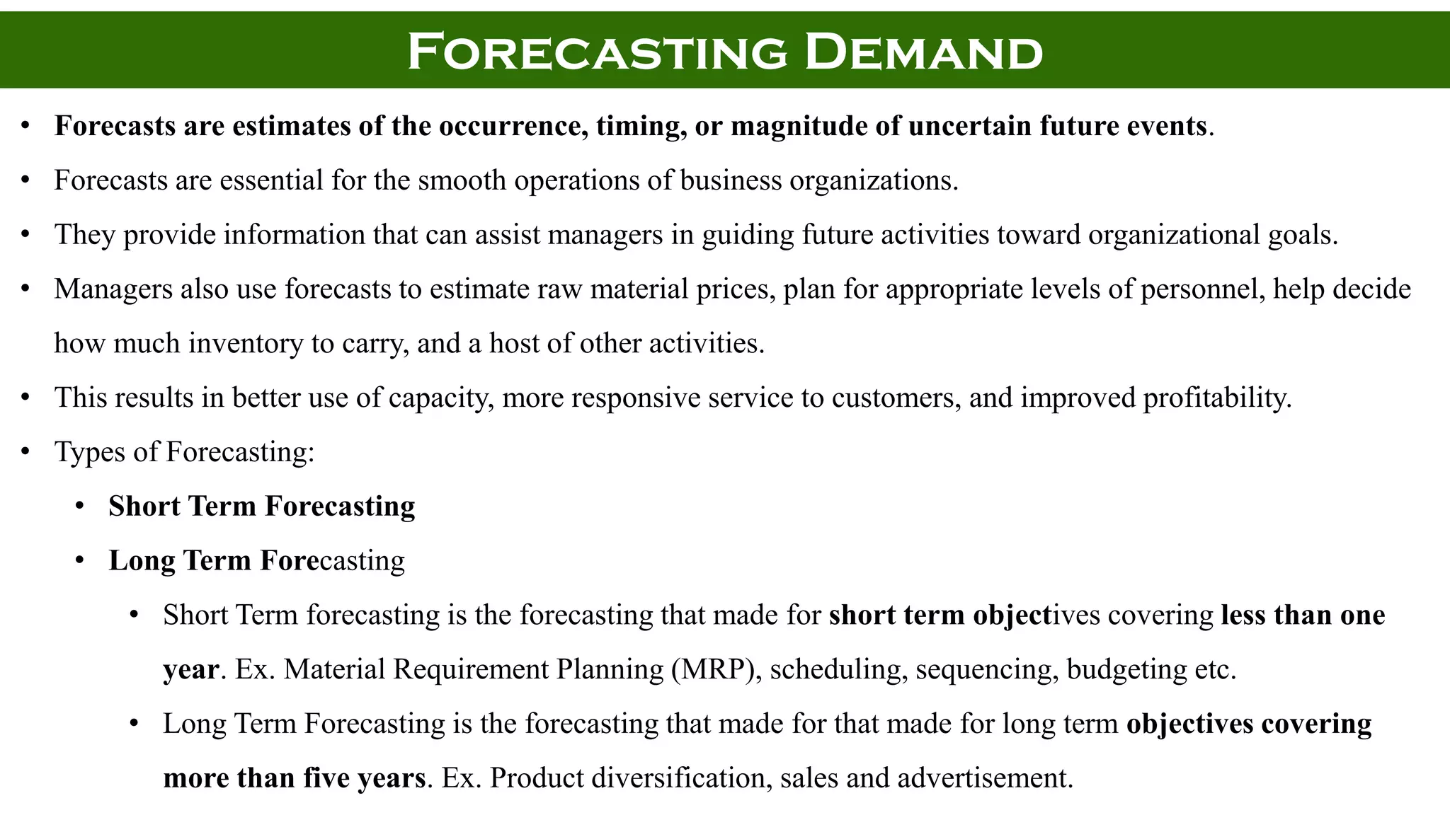
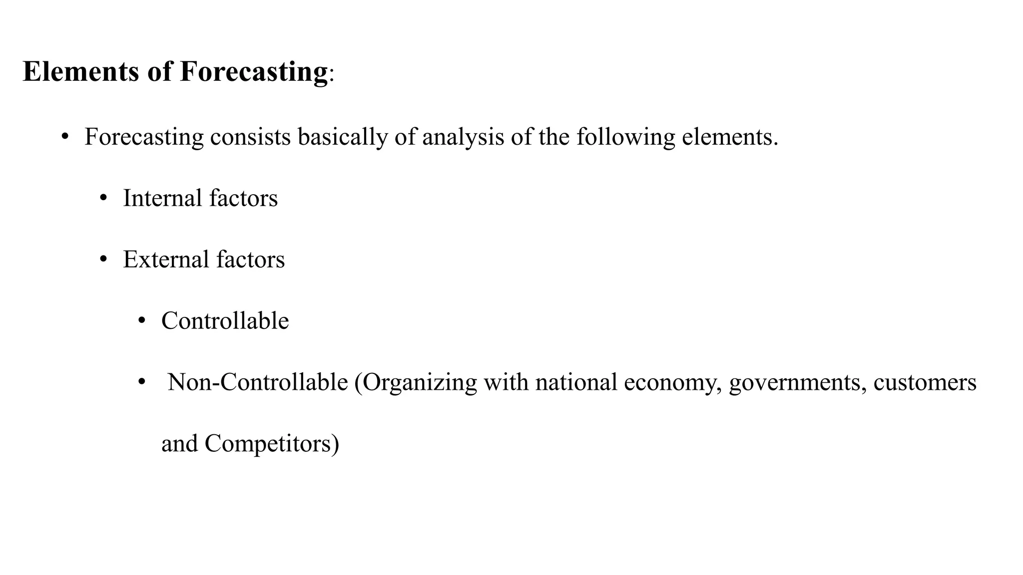
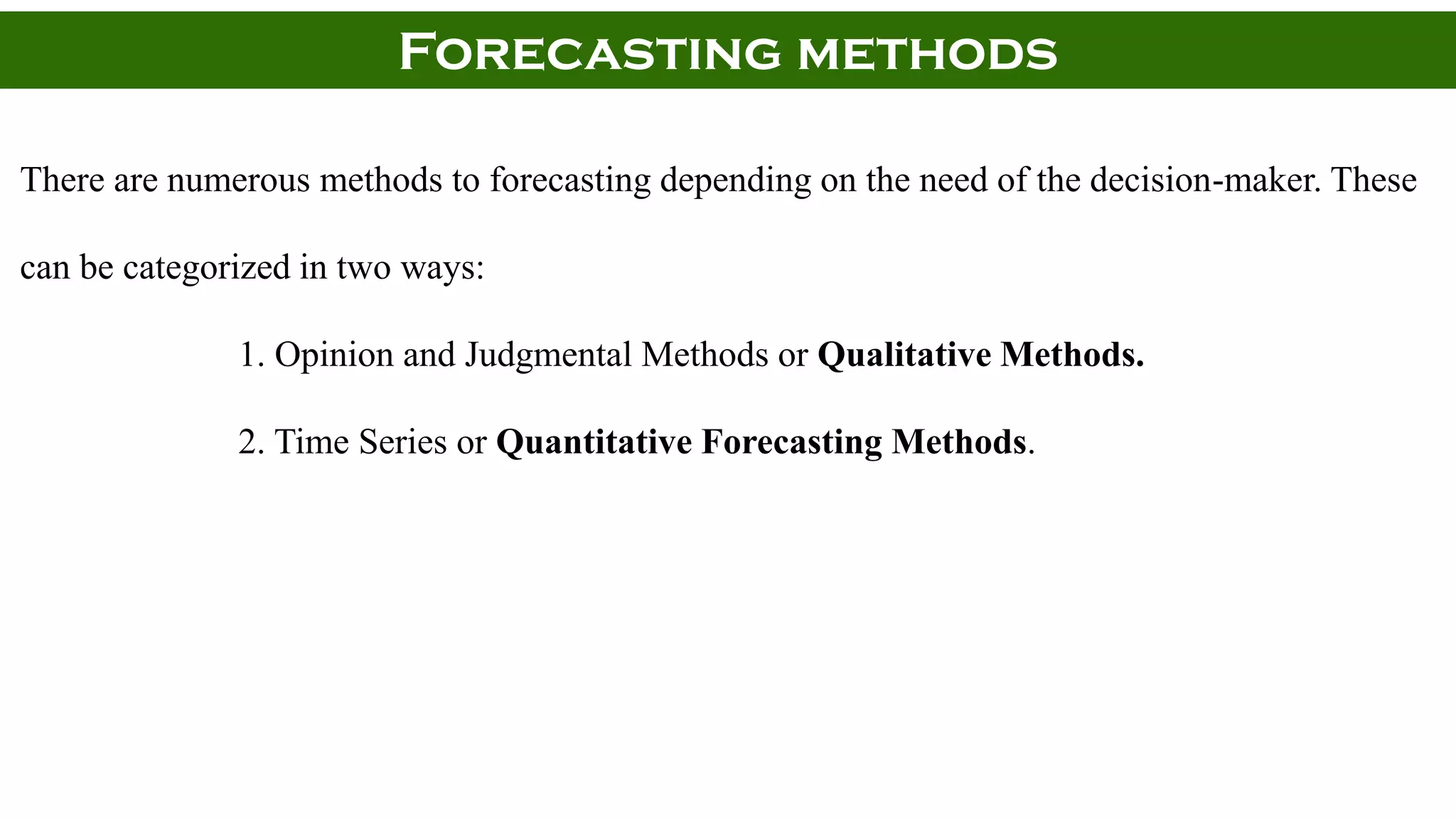
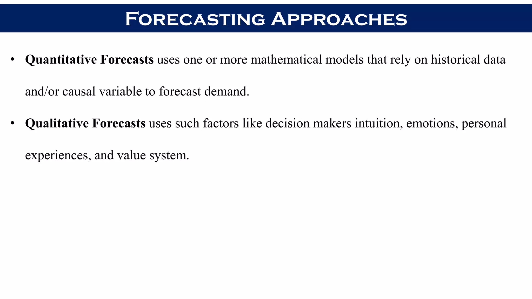
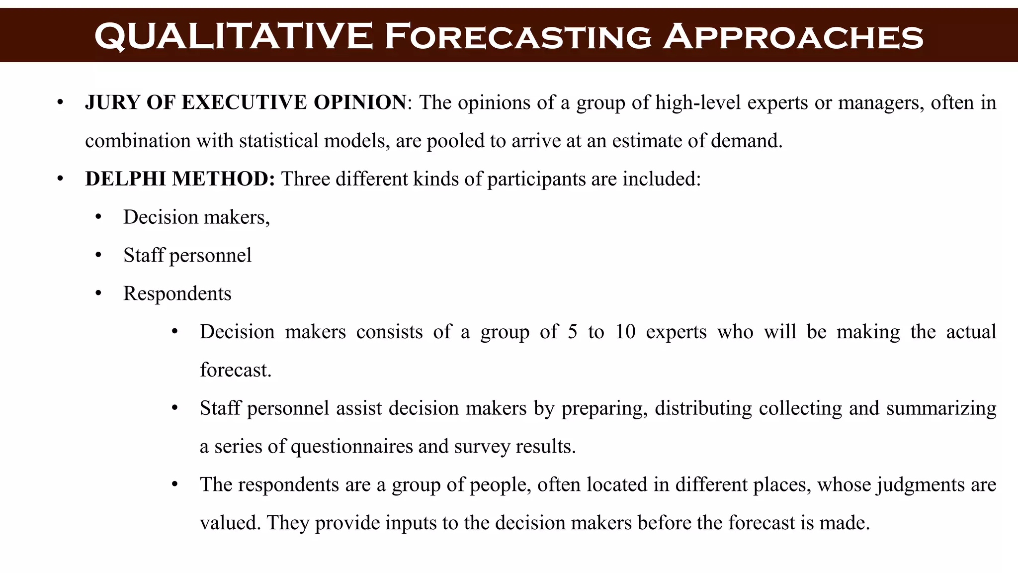
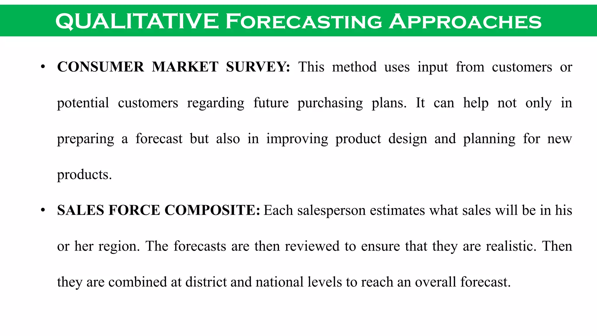
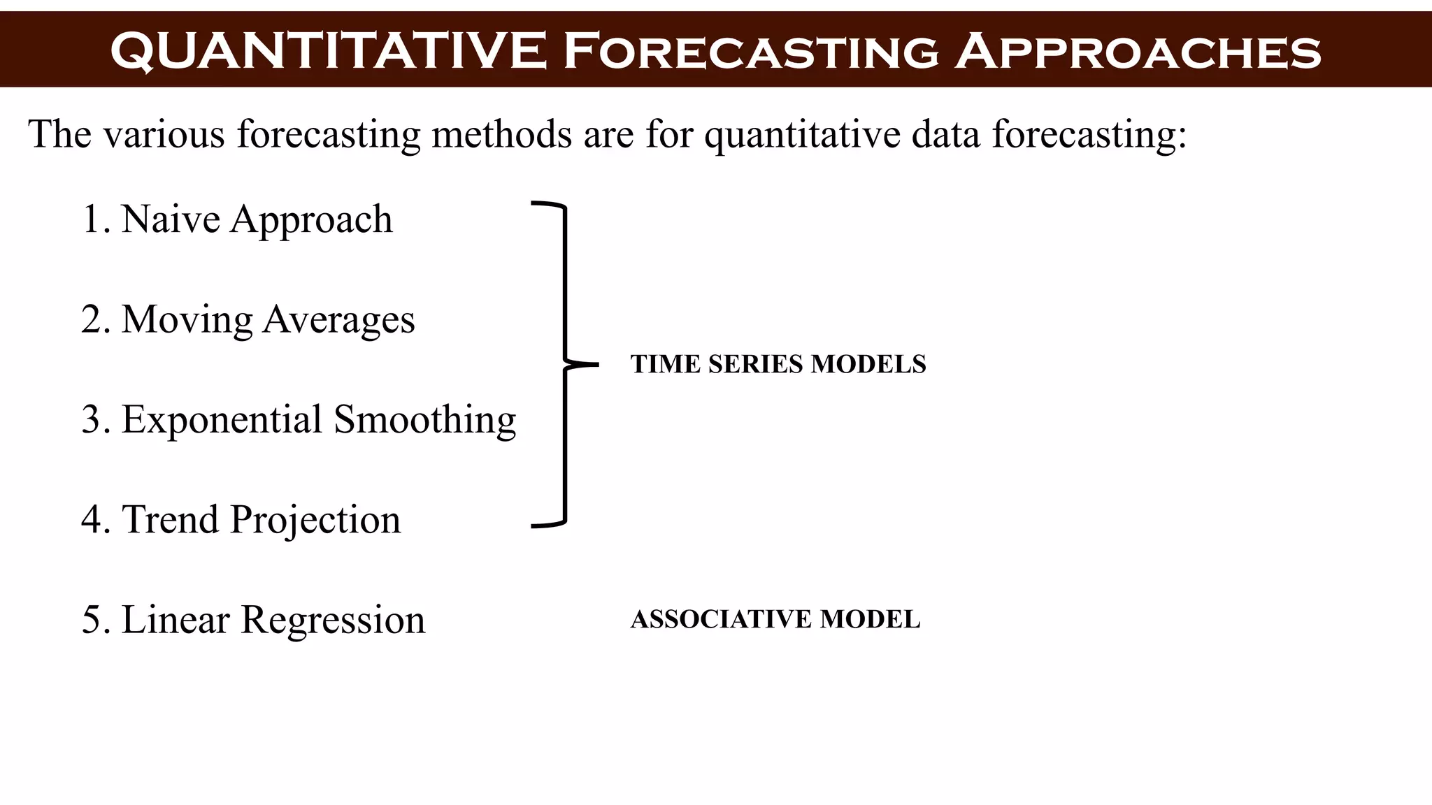
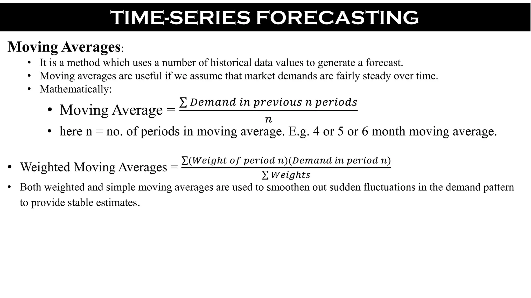
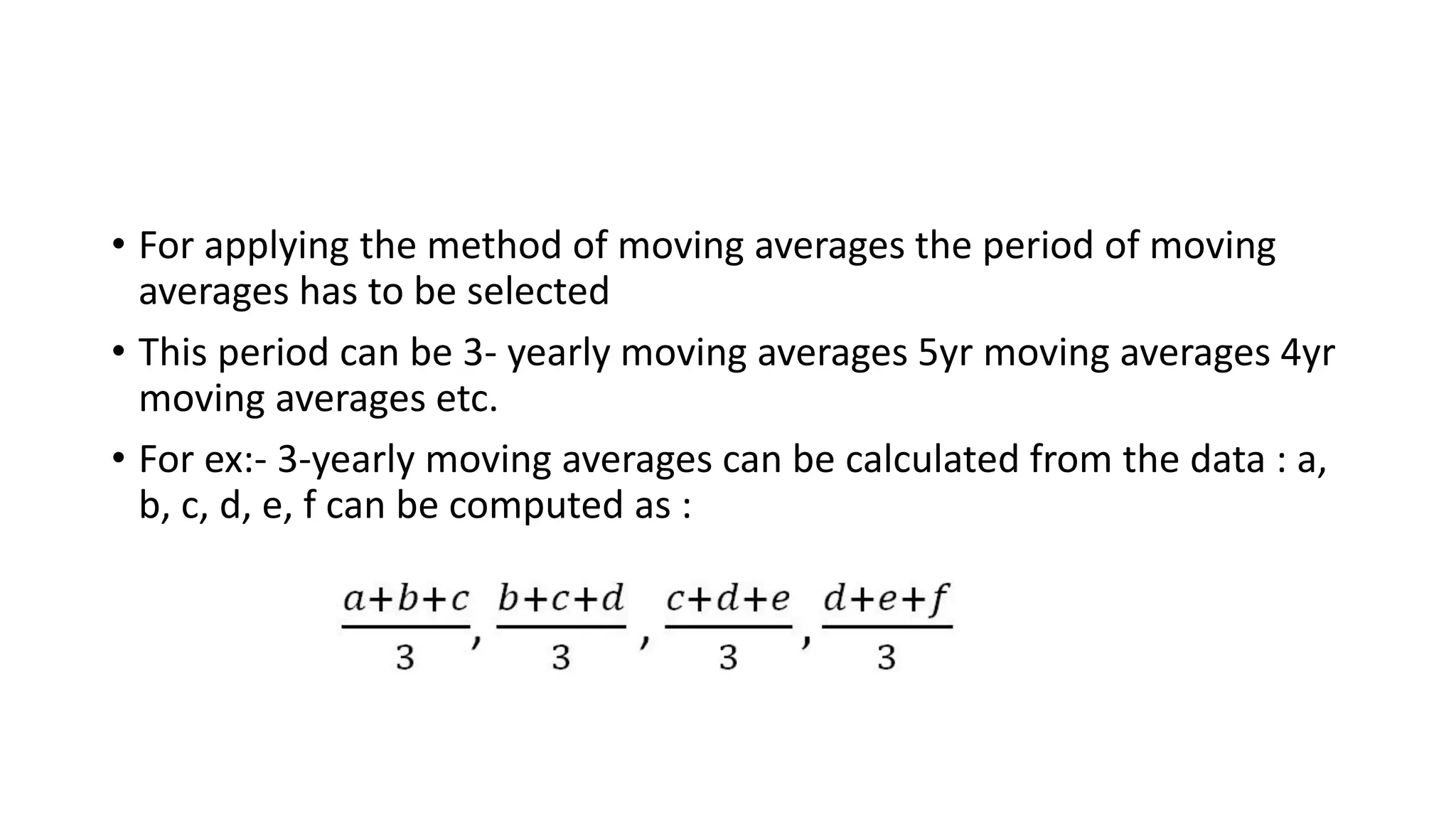
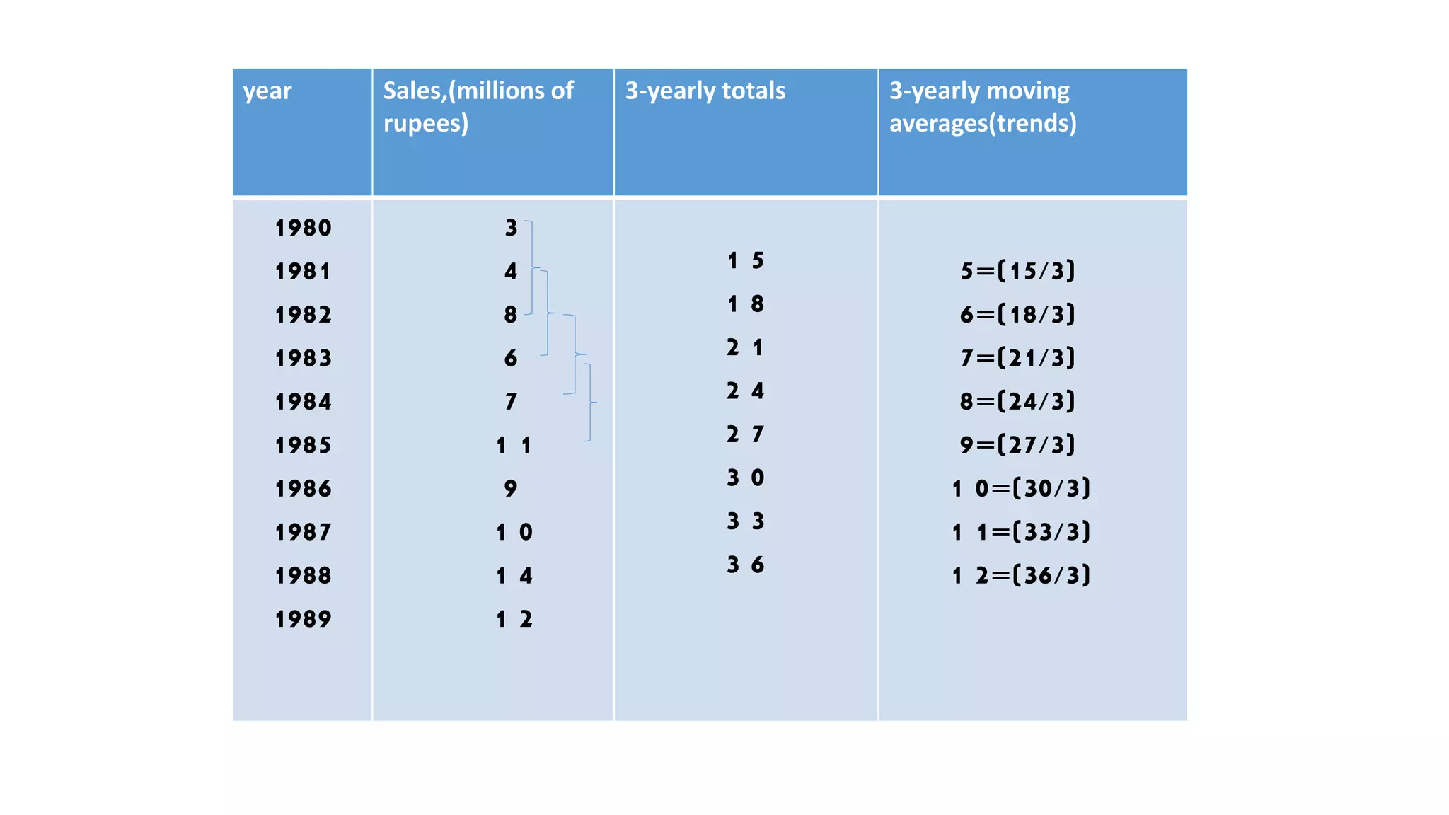
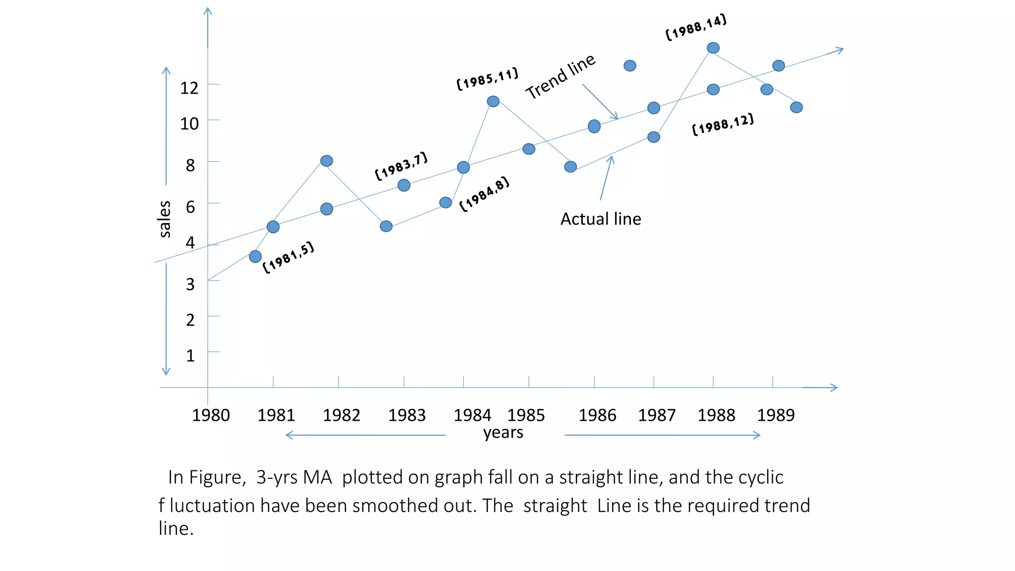
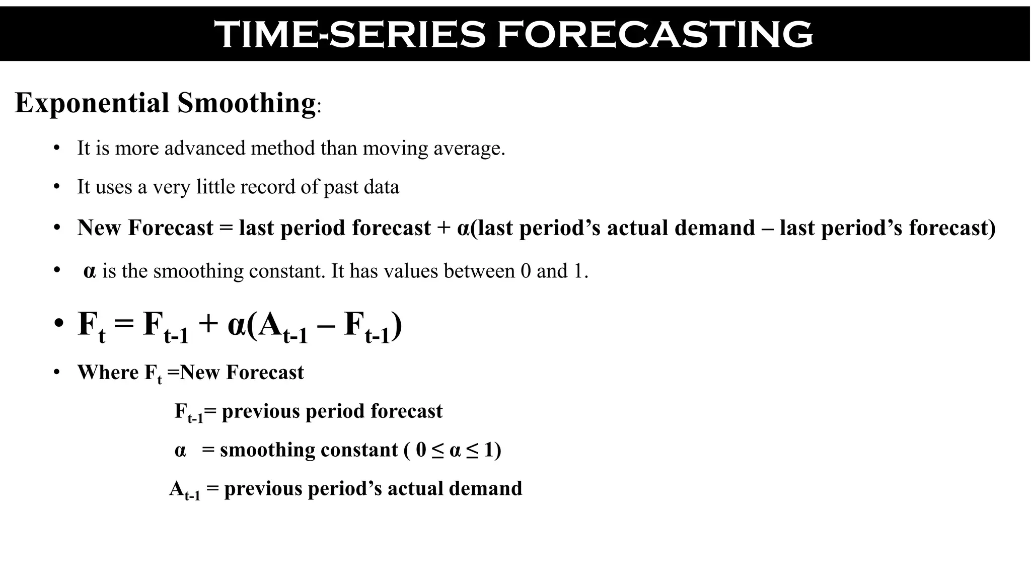
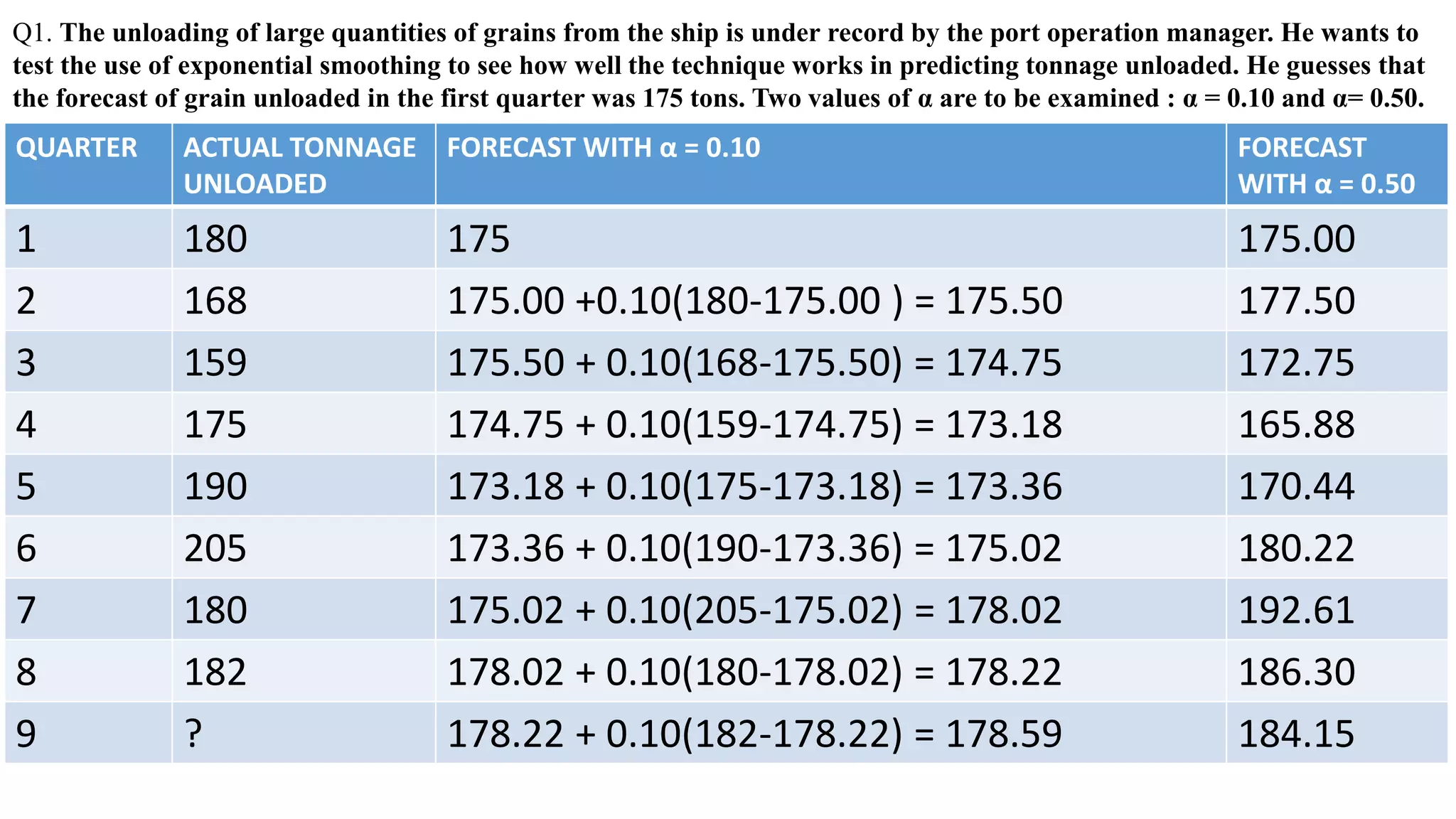
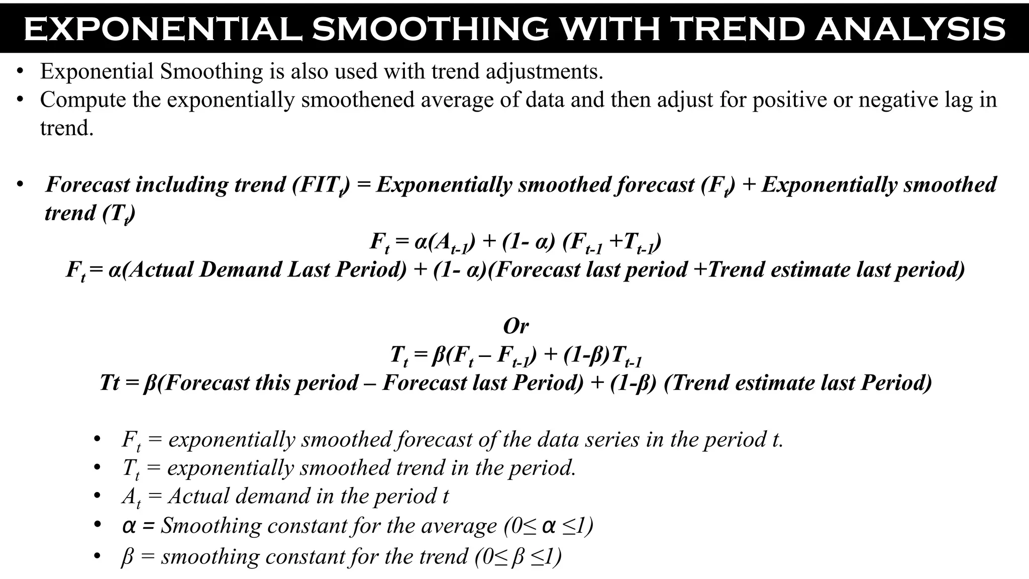
Forecasting is essential for business operations and involves estimating future events and trends. There are two main types of forecasting: quantitative and qualitative. Quantitative forecasting uses historical data and mathematical models, while qualitative forecasting relies on expert opinions. Common quantitative forecasting methods include moving averages, exponential smoothing, and time series models. Moving averages calculate the average demand over a set time period to smooth out fluctuations. Exponential smoothing places more emphasis on recent data by applying weighting factors. Qualitative methods include jury of executive opinion, Delphi method, and consumer surveys. Forecasting allows businesses to better plan operations and prepare for the future.

1. OPERATIONS MANAGEMENT
By-:
Er. Vaibhav Agarwal
Asst. Prof.
SOM, BBDU
Lucknow
FORECASTING

2. Forecasting Demand
• Forecasts are estimates of the occurrence, timing, or magnitude of uncertain future events.
• Forecasts are essential for the smooth operations of business organizations.
• They provide information that can assist managers in guiding future activities toward organizational goals.
• Managers also use forecasts to estimate raw material prices, plan for appropriate levels of personnel, help decide
how much inventory to carry, and a host of other activities.
• This results in better use of capacity, more responsive service to customers, and improved profitability.
• Types of Forecasting:
• Short Term Forecasting
• Long Term Forecasting
• Short Term forecasting is the forecasting that made for short term objectives covering less than one
year. Ex. Material Requirement Planning (MRP), scheduling, sequencing, budgeting etc.
• Long Term Forecasting is the forecasting that made for that made for long term objectives covering
more than five years. Ex. Product diversification, sales and advertisement.

3. Elements of Forecasting:
• Forecasting consists basically of analysis of the following elements.
• Internal factors
• External factors
• Controllable
• Non-Controllable (Organizing with national economy, governments, customers
and Competitors)

4. Forecasting methods
There are numerous methods to forecasting depending on the need of the decision-maker. These
can be categorized in two ways:
1. Opinion and Judgmental Methods or Qualitative Methods.
2. Time Series or Quantitative Forecasting Methods.

5. Forecasting Approaches
• Quantitative Forecasts uses one or more mathematical models that rely on historical data
and/or causal variable to forecast demand.
• Qualitative Forecasts uses such factors like decision makers intuition, emotions, personal
experiences, and value system.

6. QUALITATIVE Forecasting Approaches
• JURY OF EXECUTIVE OPINION: The opinions of a group of high-level experts or managers, often in
combination with statistical models, are pooled to arrive at an estimate of demand.
• DELPHI METHOD: Three different kinds of participants are included:
• Decision makers,
• Staff personnel
• Respondents
• Decision makers consists of a group of 5 to 10 experts who will be making the actual
forecast.
• Staff personnel assist decision makers by preparing, distributing collecting and summarizing
a series of questionnaires and survey results.
• The respondents are a group of people, often located in different places, whose judgments are
valued. They provide inputs to the decision makers before the forecast is made.

7. QUALITATIVE Forecasting Approaches
• CONSUMER MARKET SURVEY: This method uses input from customers or
potential customers regarding future purchasing plans. It can help not only in
preparing a forecast but also in improving product design and planning for new
products.
• SALES FORCE COMPOSITE: Each salesperson estimates what sales will be in his
or her region. The forecasts are then reviewed to ensure that they are realistic. Then
they are combined at district and national levels to reach an overall forecast.

8. QUANTITATIVE Forecasting Approaches
The various forecasting methods are for quantitative data forecasting:
1. Naive Approach
2. Moving Averages
3. Exponential Smoothing
4. Trend Projection
5. Linear Regression
TIME SERIES MODELS
ASSOCIATIVE MODEL

9. QUANTITATIVE Forecasting Approaches
TIME SERIES MODELS:
• A time series is a set of observations of a variable at regular intervals over time. In decomposition analysis, the components of a time
series are generally classified as trend T, cyclical C, seasonal S, and random or irregular R.
• Time series are tabulated or graphed to show the nature of the time dependence. The forecast value (Ye) is commonly expressed as a
multiplicative or additive function of its components; examples here will be based upon the commonly used multiplicative model.
• YC =T. S. C. R multiplicative model
• YC =T + S+ C+ R additive model
• Where T is Trend, S is Seasonal, C is Cyclical, and R is Random components of a series.
• Trend is a gradual long-term directional movement in the data (growth or decline).
• Seasonal effects are similar variations occurring during corresponding periods, e.g., December retail sales. Seasonal can be quarterly,
monthly, weekly, daily, or even hourly indexes.
• Cyclical factors are the long-term swings about the trend line. They are often associated with business cycles and may extend out to
several years in length.
• Random component are sporadic (unpredictable) effects due to chance and unusual occurrences. They are the residual after the trend,
cyclical, and seasonal variations are removed.

10. Components of a Time Series
• A time series can consist of five components.
• Horizontal or Stationary – Fluctuations around a
constant mean.
• Long - term trend (T).
• Cyclical effect (C).
• Seasonal effect (S).
• Random variation (R).
A trend is a long term relatively
smooth pattern or direction, that
persists usually for more than one year.
Quantity
Time

11. A cycle is a wavelike pattern describing
a long term behavior (for more than one
year).
Cycles are seldom regular, and often appear in
combination with other components.
6/90 6/93 6/96 6/99 6/02
6/97 12/97 6/98 12/98 6/99
The seasonal component of the time series exhibits
a short term (less than one year) calendar repetitive
behavior.

12. Random variation comprises the irregular unpredictable changes in
the time series.
It tends to hide the other (more predictable)
components.
Random or Irregular Variation –classified into:
•Episodic – unpredictable but identifiable
•Residual – also called chance fluctuation and
unidentifiable

13. TIME-SERIES FORECASTING
• Associative Models: Models like linear regression, incorporate the variables or factors that might influence the
quantity being forecast. E.g. Advertising budget, competitors price etc.
• A time series is based on a sequence of evenly spaced (weekly, monthly, quarterly, an so on) data points.
• E.g. including weekly sales of Nike Air Jordans, quarterly earning reports of Microsoft stocks etc.
• Forecasting time-series data implies that future values are predicted only from pat values and that other variables.

14. TIME-SERIES FORECASTING
Naive Approach:
• It is simplest way to forecast.
• It is a technique that assumes demand in the next period is equal to demand in the most recent period.

16. TIME-SERIES FORECASTING
Moving Averages:
• It is a method which uses a number of historical data values to generate a forecast.
• Moving averages are useful if we assume that market demands are fairly steady over time.
• Mathematically:
• Moving Average =
𝐷𝑒𝑚𝑎𝑛𝑑 𝑖𝑛 𝑝𝑟𝑒𝑣𝑖𝑜𝑢𝑠 𝑛 𝑝𝑒𝑟𝑖𝑜𝑑𝑠
𝑛
• here n = no. of periods in moving average. E.g. 4 or 5 or 6 month moving average.
• Weighted Moving Averages =
(𝑊𝑒𝑖𝑔ℎ𝑡 𝑜𝑓 𝑝𝑒𝑟𝑖𝑜𝑑 𝑛)(𝐷𝑒𝑚𝑎𝑛𝑑 𝑖𝑛 𝑝𝑒𝑟𝑖𝑜𝑑 𝑛)
𝑊𝑒𝑖𝑔ℎ𝑡𝑠
• Both weighted and simple moving averages are used to smoothen out sudden fluctuations in the demand pattern
to provide stable estimates.

17. Moving average method
• A quantitative method of forecasting or smoothing a
time series by averaging each successive group (no. of
observations) of data values.
• term MOVING is used because it is obtained by summing
and averaging the values from a given no of periods,
each time deleting the oldest value and adding a new
value.

18. • For applying the method of moving averages the period of moving
averages has to be selected
• This period can be 3- yearly moving averages 5yr moving averages 4yr
moving averages etc.
• For ex:- 3-yearly moving averages can be calculated from the data : a,
b, c, d, e, f can be computed as :

19. • If the moving average is an odd no of values e.g., 3
years, there is no problem of centring it. Because the
moving total for 3 years average will be centred besides
the 2nd year and for 5 years average be centred besides
3rd year.
• But if the moving average is an even no, e.g., 4 years
moving average, then the average of 1st 4 figures will
be placed between 2nd and 3rd year.
• This process is called centering of the averages. In case
of even period of moving averages, the trend values
are obtained after centering the averages a second
time.

20. Goals : –
• Smooth out the short-term fluctuations.
• Identify the long-term trend.

21. MERITS Of Moving average method
• simple method.
• flexible method.
OBJECTIVE :-
• If the period of moving averages coincides with the period
of cyclic fluctuations in the data , such fluctuations are
automatically eliminated
• This method is used for determining seasonal, cyclic and
irregular variations beside the trend values.

22. LIMITATIONS OF MOVING AVERAGE METHOD
• No trend values for some year.
• M.A is not represented by mathematical function - not helpful in
forecasting and predicting.
• The selection of the period of moving average is a difficult task.
• In case of non-linear trend the values obtained by this method are
biased in one or the other direction.

23. Moving Average Example
Year Units Moving
1994 2
1995 5 3
1996 2 3
1997 2 3.67
1998 7 5
1999 6
John is a building contractor with a record of a total
of 24 single family homes constructed over a 6-year
period. Provide John with a 3-year moving average
graph.
Avg.

24. year Sales,(millions of
rupees)
3-yearly totals 3-yearly moving
averages(trends)
1980
1981
1982
1983
1984
1985
1986
1987
1988
1989
3
4
8
6
7
1 1
9
1 0
1 4
1 2
1 5
1 8
2 1
2 4
2 7
3 0
3 3
3 6
5=(15/3)
6=(18/3)
7=(21/3)
8=(24/3)
9=(27/3)
1 0=(30/3)
1 1=(33/3)
1 2=(36/3)

25. In Figure, 3-yrs MA plotted on graph fall on a straight line, and the cyclic
f luctuation have been smoothed out. The straight Line is the required trend
line.
1980 1981 1982 1983 1984 1985 1986 1987 1988 1989
1
2
3
years
sales
4
6
8
10
12
Actual line

26. TIME-SERIES FORECASTING
Exponential Smoothing:
• It is more advanced method than moving average.
• It uses a very little record of past data
• New Forecast = last period forecast + α(last period’s actual demand – last period’s forecast)
• α is the smoothing constant. It has values between 0 and 1.
• Ft = Ft-1 + α(At-1 – Ft-1)
• Where Ft =New Forecast
Ft-1= previous period forecast
α = smoothing constant ( 0 ≤ α ≤ 1)
At-1 = previous period’s actual demand

27. Q1. The unloading of large quantities of grains from the ship is under record by the port operation manager. He wants to
test the use of exponential smoothing to see how well the technique works in predicting tonnage unloaded. He guesses that
the forecast of grain unloaded in the first quarter was 175 tons. Two values of α are to be examined : α = 0.10 and α= 0.50.
QUARTER ACTUAL TONNAGE
UNLOADED
FORECAST WITH α = 0.10 FORECAST
WITH α = 0.50
1 180 175 175.00
2 168 175.00 +0.10(180-175.00 ) = 175.50 177.50
3 159 175.50 + 0.10(168-175.50) = 174.75 172.75
4 175 174.75 + 0.10(159-174.75) = 173.18 165.88
5 190 173.18 + 0.10(175-173.18) = 173.36 170.44
6 205 173.36 + 0.10(190-173.36) = 175.02 180.22
7 180 175.02 + 0.10(205-175.02) = 178.02 192.61
8 182 178.02 + 0.10(180-178.02) = 178.22 186.30
9 ? 178.22 + 0.10(182-178.22) = 178.59 184.15

28. QUA
RTER
ACTUAL
TONNAGE
UNLOADED
FORECAST
WITH α =
0.10
ABSOLUTE
DEVIATION FOR
α = 0.10
FORECAST WITH α =
0.50
ABSOLUTE DEVIATION
FOR α = 0.50
1 180 175 5.00 175.00 5.00
2 168 175.50 7.50 177.50 9.50
3 159 174.75 15.75 172.75 13.75
4 175 173.18 1.82 165.88 9.12
5 190 173.36 16.64 170.44 19.56
6 205 175.02 29.98 180.22 24.78
7 180 178.02 1.98 192.61 12.61
8 182 178.22 3.78 186.30 4.30
TOTAL = 82.45 TOTAL = 98.62
MAD =
𝑫𝑬𝑽𝑰𝑨𝑻𝑰𝑶𝑵𝑺
𝒏
= 10.31 12.33

29. TIME-SERIES FORECASTING
Mean Squared Error: The mean squared error (MSE) is the average of the
second differences between the forecasted and observed values
MEAN ABSOLUTE DEVIATION: The first measure of the overall forecast error for a model is the mean
absolute deviation (MAD).
MAE =
𝑭𝒐𝒓𝒆𝒄𝒂𝒔𝒕 𝑬𝒓𝒓𝒐𝒓𝒔 2
𝒏

30. TIME-SERIES FORECASTING
Measuring the forecasting Error:
• Comparing forecasted values with the actual or observed values.
• It uses a very little record of past data
• Forecast Error = Actual Demand – Forecast Values
• Fe = At - Ft
• Where Ft = Forecast demand for period t
At = Actual Demand
MEAN ABSOLUTE DEVIATION: The first measure of the overall forecast error for a model is the mean
absolute deviation (MAD).
MAD =
𝑨𝑪𝑻𝑼𝑨𝑳 −𝑭𝑶𝑹𝑬𝑪𝑨𝑺𝑻
𝒏

31. EXPONENTIAL SMOOTHING WITH TREND ANALYSIS
• Exponential Smoothing is also used with trend adjustments.
• Compute the exponentially smoothened average of data and then adjust for positive or negative lag in
trend.
• Forecast including trend (FITt) = Exponentially smoothed forecast (Ft) + Exponentially smoothed
trend (Tt)
Ft = α(At-1) + (1- α) (Ft-1 +Tt-1)
Ft = α(Actual Demand Last Period) + (1- α)(Forecast last period +Trend estimate last period)
Or
Tt = β(Ft – Ft-1) + (1-β)Tt-1
Tt = β(Forecast this period – Forecast last Period) + (1-β) (Trend estimate last Period)
• Ft = exponentially smoothed forecast of the data series in the period t.
• Tt = exponentially smoothed trend in the period.
• At = Actual demand in the period t
• α = Smoothing constant for the average (0≤ α ≤1)
• β = smoothing constant for the trend (0≤ β ≤1)

37. TREND PROJECTIONS
• This technique fits a trend line to a series of historical data points and then projects the line into the future for medium to
long-range forecasts.
• A least square method is used to develop a trend line.
• It has a y-intercept and a slope.
• It can be expressed in a equation
• 𝒚 = a +bx
• Where 𝒚 = computed value of the variable to be predicted (called the dependent variable)
• a = y-axis intercept.
• b = slope of the regression line (or the rate of change in y for given changes in x)
• x = the independent variable (which in this case is time).
• Now we have to calculate the value of ‘a’ and ‘b’ constants.
• b =
𝒙𝒚 −𝒏 𝒙 𝒚
𝒙 𝟐
−𝒏 𝒙 𝟐
• a = 𝒚 − 𝒃 𝒙

38. ASSOCIATIVE FORECASTING METHODS:
REGRESSION ANALYSIS
• Regression model considers the several variables that are related to the quantity being predicted.
• It consists of a dependent variable and an independent variable.
• It may express the relation between sales volume and revenue generated.
• A least square method is used to develop a trend line.
• It has a y-intercept and a slope.
• It can be expressed in a equation
• 𝒚 = a +bx
• Where 𝒚 = computed value of the variable to be predicted (called the dependent variable)
• a = y-axis intercept.
• b = slope of the regression line (or the rate of change in y for given changes in x)
• x = the independent variable (which in this case is time).
• Now we have to calculate the value of ‘a’ and ‘b’ constants.
• b =
𝒙𝒚 −𝒏 𝒙 𝒚
𝒙 𝟐
−𝒏 𝒙 𝟐
• a = 𝒚 − 𝒃 𝒙

39. Note:
1. Solve the numerical questions on the topic of Exponential Smoothing,
Moving Averages, Trend Projection and Regression analysis from the text
book.
2. This topic is numerical based topic and numerical portion is very very
important. So practice well for the numerical portion.

40. THANK YOU
References:
1. Kumar, S. Anil; Suresh, N., ‘Operations Management’, New Age International Publishers, 2e.
2. Heizer, Jay; Render, Barry; Rajashekhar, Jagadeesh, ‘Operations Management’, Pearson, 9e.
3. Chary, S N, ‘Production & Operations Management’, McGraw-Hill Companies, 4e.
4. Ashwathappa, K.; Bhat, K. Shridhara, ‘Productions and Operations Management’, Himalaya
Publishing House, 2e.