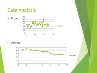
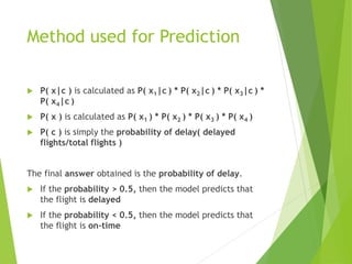
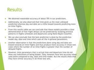
The project focuses on predicting flight departures delays using a Bayesian classification approach, addressing significant challenges in aviation due to unreliability in flight scheduling. Data from February 2008 was analyzed, with various attributes selected and prepared to identify relevant factors influencing delays. The prediction models, utilizing a Naïve Bayes classifier, achieved around 70% accuracy, revealing that including parameters such as day, date, and time improves predictive performance.

1. Flight Departure Delay Prediction
By
Kumar Gaurav(2K12/SE/038)
Vaibhav Goyal(2K12/SE/093)
Vivek Maskara(2K12/SE/097)
Minor Project Report on
Project Guide:
Mr Manoj Kumar

2. Introduction
 Flight delay creates major problems in the current
aviation system and in scheduling of airport operations,
the unreliability of flight arrivals is a serious challenge.
 Punctuality is an issue for all major carriers, with some
struggling more than others.

3. Objective
The objective of the project is to predict whether a flight will be delayed
or not by studying the various features of the flight and calculating
probability for delay using Bayesian Classification.

4. Overview
The project has gone through the following stages
1. Collection of data
2. Selection of attributes
3. Data Preparation
4. Data Analysis
5. Test Set Preparation
6. Prediction method

5. Collection of Data
1. Flight data for last 20 years is available for download
at website for Bureau of Transportation Statistics,
United States of America.
2. For this project, only data of 1 month- Feb 2008 was
considered because of the massive amount of data
available. This month too has record of more than
6,00,000 flights.

6. Selection of Attributes
 Originally there were a large number of attributes in
the original dataset.
 Many were discarded based on their irrelevance or if
they could be found through other attributes. For eg-
flight numbers, aircraft ids etc were discarded because
of this.

7. Selection of Attributes
 For analysis, 12 attributes considered –
1. Day of Month
2. Day of Week
3. Carrier
4. Origin
5. Departure Time
6. Delay minutes
7. DepDel15 – if delay is greater than 15mins
8. Cancelled
9. Diverted
10. Distance Group
11. Arrival Time
12. Destination

8. Data Preparation
1. Import data from csv(comma separated values ) files
to sql tables to make data more manageable.
2. Delete all the data about the flights that were
missing some data due to any reason like it was
diverted, cancelled or distance is less than 0 or data
provided about the flight is incomplete.

9. Data Preparation
3. Dataset is converted into discretized dataset that is
distance and departure time are converted into nominal
categories by placing them in equal width bins.
 For distance, 11 bins are used, each bin of 250 miles of
width. So distance of 0-250 miles is set as 1, 250-500
miles as 2 and so on.
 For departure time and arrival time, 6 bins are used,
each bin of 400 hours of width. So time from 0-400
hours is set as 1, 400-800 as 2 and so on.

10. Data Preparation
4. The dataset is simplified further to remove flights with
uncommon attribute values in either origin or unique
carrier. The top 25 most frequently occurring airports in
origin and destination are considered.
 The instances that do not have values within these two
groups are deleted.

11. Data Preparation
5. During the discretization of dataset in Step3, a lot of
duplicate instances are created again which have
similar values. So all these instances are also deleted
and only one of the duplicate values is kept.

12. Data Analysis
 Various attributes are analyzed to determine which
attributes are relevant in prediction of delays and which
attributes can be discarded as irrelevant.
 It is explored how the delays are distributed across
different variables. This step basically extracts the
importance of each variable in affecting the patterns in
flight departures and delays.

13. Data Analysis
 There are 8 attributes – each of them are studied
separately –
1. Day of Month
2. Day Of Week
3. Unique Carrier
4. Origin
5. Departure Time
6. Distance Group
7. Arrival Time
8. Destination
4 of these attributes are used in all types of prediction

14. Data Analysis
 Day of week
 Unique Carrier
0
10
20
30
40
50
0 2 4 6 8
Series1
0
10
20
30
40
50
60
AA DL MQ OO UA US WN XE
Series1

15. Data Analysis
 Origin
 Distance
0
10
20
30
40
50
60
70
0 10 20 30
Series1
0
10
20
30
40
50
0 2 4 6 8 10 12
Series1

16. Test Sets Preparation
 In all, 3 test cases are created based on the ratio of
number of delayed flights to number of on-time
flights:
1. Ratio is 1:1
2. Ratio is 1:3
3. Ratio is 3:1

17. Types Of Prediction
After exploring these relationships, we now make 7
prediction models on the basis of 4 parameters. The models
are –
 Day
 Date
 Time
 Day and date
 Date and time
 Day and Time
 Day, Date and Time

18. Method used for Prediction
 Naïve Bayes Classifier is used for predicting the delays.
 It uses the following formula for calculating the
probability of an event.

19. Method used for Prediction
 P(c|x) is the posterior probability of class (target)
given predictor (attribute).
 P(c) is the prior probability of class.
 P(x|c) is the likelihood which is the probability
of predictor given class.
 P(x) is the prior probability of predictor.

20. Method used for Prediction
 P( x|c ) is calculated as P( x1|c ) * P( x2|c ) * P( x3|c ) *
P( x4|c )
 P( x ) is calculated as P( x1 ) * P( x2 ) * P( x3 ) * P( x4 )
 P( c ) is simply the probability of delay( delayed
flights/total flights )
The final answer obtained is the probability of delay.
 If the probability > 0.5, then the model predicts that
the flight is delayed
 If the probability < 0.5, then the model predicts that
the flight is on-time

21. Method used for Prediction
 For prediction of the delay minutes, delay classes have
been established and delay minutes are predicted on
the basis of the probability of delay.
 These classes show the range of delay minutes on the
basis of the range of probability
 The range of these classes have been established on the
basis of training set data by calculating the highest,
lowest and median values for a probability range.
 In all there are 10 classes, the range of each class being
10 minutes.

22. Results
Prediction Model TestSet
(Ratio – delayed:on-time)
No of delayed
flights
No of on-time flights Predicted delayed
flights
Predicted on-time
flights
Accuracy
Time TestSet1(3:1) 250 750 435 565 58.5
Time TestSet2(1:1) 500 500 536 474 64.6
Time TestSet3(1:3) 750 250 576 424 61.5
Day and date TestSet1(3:1) 250 750 245 755 69.3
Day and date TestSet2(1:1) 500 500 267 733 581
Day and date TestSet3(1:3) 750 250 322 678 47.4
Day and time TestSet1(3:1) 250 750 264 736 69.2
Day and time TestSet2(1:1) 500 500 313 687 60.3
Day and time TestSet3(1:3) 750 250 415 585 54.9
Date and time TestSet1(3:1) 250 750 232 768 73.2
Date and time TestSet2(1:1) 500 500 312 688 61.0
Date and time TestSet3(1:3) 750 250 376 624 53.4
Day, date and time TestSet1(3:1) 250 750 232 768 74.6
Day, date and time TestSet2(1:1) 500 500 305 695 64.5
Day, date and time TestSet3(1:3) 750 250 390 610 54.4

23. Results
 We obtained reasonable accuracy of about 70% in our predictions.
 Additionally, we also observed that time gives us the most unbiased
prediction whereas day and date are a little biased towards predicting more
on-time flights.
 From this results table we can conclude that these models provides a clear
demonstration of how flight delays can be predicted by studying previous
patterns in flights schedules and departures using Naïve Bayes Classifier.
 We can also conclude that the best prediction is done by the prediction
model day, date and time which uses all the 4 optional parameters.
 Another observation is that the predictions done using day and date are
biased towards on-time flights and thus produce more accuracy in those test
cases where the number of on-time flights is greater than the number of
delayed flights.
 However, time parameters that is arrival time and departure time do not
show any indications of being biased. They, however have less accuracy when
used alone compared to day, date and time model. But the results show that
they have similar accuracy in all three test sets.