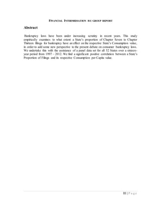
This document is a 5960 word independent study report that examines whether the proportion of Chapter 7 to Chapter 13 bankruptcy filings in the USA influences consumption levels. It contains an introduction outlining the research question, a literature review of previous related studies, a description of the economic framework and methodology, an analysis of the results, and conclusions. The key findings are that a significant positive correlation was found between a state's proportion of bankruptcy filings and its consumption per capita, providing evidence that a higher proportion of Chapter 7 filings may be beneficial to a state's economy.
Power point slide presentation of the final projectobjectivediMARK547399
Β
The document provides guidelines for creating a PowerPoint presentation for a final project. It states that PowerPoint presentations can be a powerful tool to accompany oral presentations but must be carefully prepared to not distract from the speaker. It provides tips for the presentation such as keeping it between 7-15 slides, using readable fonts, and checking it against the grading rubric.
The document discusses two topics: reducing the federal government's discretionary powers and achieving a balanced government budget. For reducing discretionary powers, it summarizes the advocates' view that government spending is inferior to private spending and the critics' view that government spending disrupts efficient allocation of resources. For balanced budgets, it outlines the advocates' position that it increases investment and economic responsibility and the critics' argument that it ties the government's hands and could worsen recessions. The author concludes by supporting the critics' views on both topics.
The next President will need to confront a number of budgetary challenges and will likely sign into law many federal tax and spending changes. Yet too often, election campaigns are about telling voters what they want to hear rather than what they need to know. To separate fiction from reality, the new Fiscal FactChecker series will monitor the 2016 Presidential campaign on an ongoing basis. To start with, we have identified 16 myths that may come up during the campaign.
Fred Dickson, Chief Investment Strategist for DA Davidson spoke at the Southern Oregon Business Conference on January 26, 2011. While our region has some specific challenges, it is good to hear that we are avoiding a double-dip recession and we can expect to continue a slow recovery.
A primer with answers to all your questions about a federal government shutdown. Such as, What services are affected in a shutdown and how?, How would federal employees be affected?, Does a government shutdown save money?, and more.
The document discusses several topics related to financial markets in 2011 and beyond. It first looks at whether anyone can truly predict market performance based on the volatility seen in 2008. It then examines the performance of various asset classes from 2000-2010. The document also covers issues around Social Security, including myths, the current status of the trust fund, and options for reform. Finally, it discusses the growing crisis in public pension plans, comparing defined benefit and defined contribution plans, and how states are dealing with underfunding issues.
This newsletter from Cedar Point Financial Services provides information on upcoming interest rate hikes and how they could impact various financial products. It discusses how adjustable rate mortgages, credit cards, and variable rate student loans may be affected if interest rates rise. The newsletter recommends ways for readers to protect themselves, such as refinancing a mortgage, paying down credit card debt, and reviewing student loan terms. It also provides two articles on estate tax reform possibilities and the connection between health and personal finances.
1) The Congressional Budget Office presentation discusses the challenges of estimating the federal budget and economy in light of the fiscal stimulus and ongoing recovery from recession.
2) It notes that while the recovery is underway, several factors will dampen its strength, including financial market fragility and restrained household spending.
3) A key issue is that under current policies, spending for programs like Social Security and Medicare will exceed total federal revenues by 2020, meaning significant changes will be needed to taxes or other spending.
Australian economic briefing by david rumbens (1)Sebastian Cohen
Β
The document provides an economic briefing and discussion of the recently released Australian Tax Discussion Paper. It summarizes that the paper outlines the tradeoff between efficiency, equity and simplicity in any tax system. It notes that income taxes account for a large share of Australian tax revenue compared to other countries. The briefing discusses how shifting some of the tax burden from direct to indirect taxes could provide an efficiency benefit to the economy.
The document is a January 2014 newsletter from Prism Capital Management that provides investment updates on several topics:
1) It summarizes the history of interest rates in the US, noting they are currently near historic lows but expected to rise in the future.
2) It outlines the economic outlook for 2014, expecting continued slow GDP growth around 2% with little change in employment, inflation expected to increase slightly but remain low.
3) It summarizes new research from Morningstar that challenges common assumptions around retirement costs, finding actual costs are often lower than estimated based on factors like taxes, spending patterns, and life expectancies.
In preparing its baseline projections of the federal budget, CBO models the budgetary costs of programs that insure single-family mortgages. This slide deck provides an overview of that modeling approach for the largest of those programs: the Federal Housing Administration and the government-sponsored enterprises Fannie Mae and Freddie Mac.
The document discusses financial well-being and how it is defined by the Consumer Financial Protection Bureau. Financial well-being has four key components: having control over day-to-day finances, having the capacity to absorb financial shocks, being on track to meet financial goals, and having financial freedom to enjoy life. The document focuses on the first two components - having control over finances and absorbing financial shocks. It emphasizes the importance of an emergency fund and having a back-up plan for income to be prepared for unexpected expenses and job loss.
Long term budget projections, entitlements and demographicsEd Dolan
Β
The document summarizes projections of long-term US federal government debt levels over the next 50 years from the Congressional Budget Office. It discusses the different scenarios and assumptions that produce a wide range of possible debt trajectories, all of which show debt growing to unsustainable levels. The primary drivers are expected growth in entitlement programs like Social Security and Medicare due to an aging population and rising healthcare costs. Delaying fiscal adjustments to address the budget imbalance will only increase the size of changes needed in the future.
An Empirical Study to Investigate the Reasons for the Increase in the Househo...Ehsan Dehghanizadeh
Β
This paper investigates factors that affect household debt levels in Canada using a multiple linear regression model. Previous studies found GDP growth, housing prices, and unemployment and interest rates significantly impact debt levels. The study uses quarterly Canadian data from 2005 to 2014 to examine how GDP, housing prices, inflation, unemployment, and interest rates influence household debt as a percentage of GDP. It aims to determine the main drivers of rising Canadian household indebtedness and inform policy responses.
Why we will not experience a DepressionGaetan Lion
Β
- The document discusses how government interventions on an unprecedented scale, including fiscal stimulus packages, monetary policy actions, and financial industry bailouts, will help prevent another Great Depression.
- During the Great Depression, bad government policies exacerbated the situation, but current interventions aim to stimulate the economy and stabilize financial markets.
- Corporations, small businesses, and households have strong financial positions and ability to finance themselves, giving government policies time to take effect before a depression could occur.
The research paper is based on the US Fiscal Cliff deal, a the popular term to describe the expiry of tax breaks and introduction of spending cuts leading to conundrum that the US economy faced at the end of 2012
The brookings institution webinar covid 19 and the economyTatianaApostolovich
Β
With more than 1,000 deaths, 3 million and counting unemployed, and no definite end in sight, the coronavirus has upended nearly every aspect of American life. In the last two weeks, the Federal Reserve and Congress scrambled to pass policies to mitigate what will be a very deep recession. Americans across the country are askingβ what exactly is going on economically? Is the government responding effectively? How do we set ourselves up for economic recovery once the pandemic recedes? On Monday, March 30, Brookings hosted an online discussion on the current state of the economy, the federal response, and challenges for state and local governments. After the discussion, speakers answered questions from the audience. This was an exclusively virtual event that was streamed live on the Brookings website
Budget Deficit and Economic Growth in Liberia: An Empirical InvestigationAJHSSR Journal
Β
: This paper investigates the relationship between budget deficits and economic growth in Liberia.
The study employed: the Classical Ordinary Least Squares Technique (OLS); The Augmented Dickey Fuller
(ADF) and Phillip Perron unit root tests for stationarity; the Co-integration test using Engle-Granger Two-Step
procedure (EGTS); and a parsimonious Error Correction Model of the relationship between Budget deficit and
economic growth in Liberia. It is evident from the analysis that there exists a long run relationship between Budget
deficit and economic growth in Liberia. There also exists a positive and significant relationship between Budget
deficit and economic growth in Liberia. Therefore, a 1.0 percent increase in deficits will result in an increase of
approximately 0.42 percent in economic growth in Liberia. The study recommends that government, policy makers
and the monetary authorities should ensure an appropriate mix of monetary and fiscal policies such that would
deliberately and strategically maximize the growth potentials of deficits in Liberia.
JEL Classification : C2, E1, E2, O4, O5
KEYWORDS: Budget Deficit, Economic
The alaska state budget (mat su business alliance 3.21.2014)Brad Keithley
Β
The document discusses Alaska's state budget challenges, including growing spending outpacing falling revenues. It notes that without significant changes, Alaska will face a severe fiscal crisis after 2023 that will lead to an economic crash. To avoid this, the state needs to save more revenue above sustainable spending levels and restrict spending growth. The key drivers of increasing spending are K-12 education, Medicaid, and retirement assistance. The document recommends capping overall spending at sustainable levels and prioritizing programs to fit within the budget. Failing to address unsustainable spending trends will likely lead to a fiscal and economic crisis for Alaska.
Sustainable spending and state of alaska fiscal planning (alaska dialogue 9.1...Brad Keithley
Β
This document discusses two policy options for Alaska's fiscal planning and sustainable spending. Option 1 is a "business as usual" approach that will likely require new taxes like an income tax to be phased in by 2026 due to inadequate revenues to support demands on the state. Option 2 advocates for a "sustainable budget" of $5.5 billion by saving more and restricting spending growth, funneling revenues above that level into savings to avoid an economic crisis. The document notes that delaying changes to shift to a sustainable model will only make addressing the state's fiscal challenges harder for future generations.
The document discusses the growing problem of government debt in the United States. It notes that the annual deficit has grown substantially in recent years, reaching over $1 trillion in 2010 and 2011. This level of deficit requires significant government borrowing each year. The total national debt held by the public is over $10 trillion. Cutting spending, raising taxes, and economic growth are the three main strategies proposed to address the debt, but each faces challenges. The high and growing level of debt poses economic risks going forward.
The Wisconsin Retirement System (WRS) faces challenges from shifting demographics, economic uncertainty, and political threats. It provides retirement security for over 600,000 people but faces headwinds like an aging population, a potential economic downturn, and efforts to privatize or reduce the system. The Protecting Our Wisconsin Retirement Security (POWRS) organization advocates to preserve the WRS and engages the public to counter legislative proposals that could weaken retirement security.
The document discusses the fiscal cliff faced by the US economy at the end of 2012. It was caused by the simultaneous expiration of tax cuts and introduction of tax increases and spending cuts. This would have pushed the US back into recession. The fiscal cliff was not caused by typical economic crises but rather the expiration of a number of laws providing tax relief and spending measures. These automatic changes would have raised taxes and cut spending starting in 2013 without Congressional action. The fiscal cliff threatened negative impacts on the US and Indian economies through reduction in consumption, business investment, and outsourcing. It could also increase inflation in India through higher gold prices and a weaker rupee.
What is the "fiscal cliff"? It's the term being used by many to describe the unique combination of tax
increases and spending cuts scheduled to go into effect on January 1, 2013.
Este documento presenta las etapas iniciales del proceso de investigaciΓ³n, incluyendo la concepciΓ³n de una idea de investigaciΓ³n, el planteamiento del problema, y el establecimiento de objetivos claros y alcanzables. Explica que los objetivos guΓan la investigaciΓ³n y evitan desviaciones, y provee ejemplos de objetivos para un estudio sobre los factores que influyen en el desarrollo del noviazgo entre jΓ³venes. Concluye que sin objetivos no puede haber una investigaciΓ³n efectiva.
Android is an open-source software platform and operating system based on the Linux kernel. It was developed by Android Inc which was later acquired by Google in 2005. Android allows developers to use its source code to develop applications and is managed by the Open Handset Alliance consortium of technology companies. It supports communication over cellular data networks as well as WiFi and Bluetooth. Key features include customizable interfaces, access to millions of apps, and support for various media formats.
This document contains the resume of Ashutosh Kulkarni. He has over 19 years of experience in business analysis, project management, and test management. He is proficient with Oracle applications and has experience working with clients in various industries like manufacturing, finance, logistics, and more. Currently he works as an Associate Consultant at Tata Consultancy Services where he is involved in projects like Oracle application software support, BI migrations, and production support.
La mejora continua debe ser un esfuerzo permanente de todos los involucrados en una estructura operativa y administrativa para mejorar los productos, servicios, y procesos de una organizaciΓ³n, es decir trabajo en equipo; considerando que las economΓas y las necesidades de los clientes estΓ‘n en constante evoluciΓ³n y globalizaciΓ³n, por lo que es indispensable evaluar los indicadores para la correcta toma de decisiones en la soluciΓ³n de problemas contribuyendo de esta manera a la mejora continua de la organizaciΓ³n.
This document outlines the sections and contents of a typical business plan, including an executive summary, marketing, legal, operations, financials, risk management, and appendices. The executive summary describes the business, goals, value proposition, and management team. The marketing section covers market analysis, strategies, and tactics. Legal covers structure, agreements, and investors. Operations addresses facilities, staffing, suppliers, and production. Financials include funding requests, budgets, projections, costs, and financing. Risk management evaluates threats and uncertainties. Appendices contain supporting documents. Work products range from a 10-20 slide pitch deck to a full multi-page business plan.
Informatica iv material para actividad 7Arucellly BR
Β
Este documento proporciona sugerencias para crear una presentaciΓ³n eficaz, incluyendo reducir el nΓΊmero de diapositivas, elegir un estilo y tamaΓ±o de fuente legible desde la distancia, simplificar el texto con viΓ±etas o frases cortas, utilizar elementos grΓ‘ficos para transmitir el mensaje pero sin sobrecargar las diapositivas, agregar etiquetas claras para grΓ‘ficos y diagramas, elegir fondos tenues y coherentes, utilizar un alto contraste entre el fondo y el texto, y revisar la ortografΓa y gramΓ‘tica
This document discusses two blog types that Indigo Blog Creations offers - a personal blog to share views and a business blog to share services. Indigo Blog Creations helps users create blogs either for personal use to post opinions and perspectives or to promote business services and offerings.
This document summarizes the design process of a bio-inspired walking robot. It began with four conceptual designs, two using one servo and two using multiple servos. After analysis, a design mimicking a seal gait was selected as the simplest. Statics and kinematics analysis determined a 2:1 gear ratio was needed to provide sufficient torque. The robot was built, but initially the servo could not handle the weight. Weight was reduced and arm lengths adjusted, allowing it to successfully walk 4.9 meters as required. The analysis upfront helped produce a simple, robust design that performed well.
Este catΓ‘logo de productos presenta a ASUS como la segunda marca lΓder mundial en notebooks de consumo. Resalta que ASUS diseΓ±a una amplia gama de productos como notebooks, monitores, tarjetas grΓ‘ficas, entre otros. AdemΓ‘s, destaca algunos modelos especΓficos de notebooks como la serie G752 y Zenbook UX501.
This document discusses how Drupal and HTML5 can work together. It describes the benefits of classic Drupal applications and HTML5 applications. Classic Drupal apps have everything contained on the server, while HTML5 apps download everything to the client and run locally using JavaScript frameworks. Using Drupal as a backend with a JSON REST interface provides content and user management for HTML5 apps. The future of Drupal 8 may include more support for HTML5 features and frameworks.
The document discusses implementing a two-pronged approach to connecting applications and data sources across an enterprise using a middleware platform and APIs. The approach aims to provide loose coupling between systems for flexibility and plug-and-play connectivity through self-service APIs to enable faster delivery. A canonical data model is proposed to allow decoupling from different data formats and an enterprise API portal is suggested to expose data and functionality through a centralized access point for various consumer applications.
Translation of the Meanings of The Noble Quran in the Spanish (Espanol) Langu...The Choice
Β
This Spanish (Espanol) translation was sponsored by the Saudi government and is provided free.
Publisher: King Fahd Complex For The Printing Of The Holy Qurβan Madinah, K.S.A.
The Industrial Marketing and Purchasing IMP ModelAbdinasir Ali
Β
The Industrial Marketing and Purchasing IMP Model
The IMP Model consists of:1) Interaction Process2) Interaction Parties3) Interaction Environment4) Atmosphere
Apart from residential spaces communities consist of various public and semi-public spaces for varied activities. It is public and gathering spaces where community comes to life. The best gathering space will be alive with activity a people of various ages, interacting with each other.
The public spaces are designed by keeping in mind the entertainment and satisfaction of the people relating to the ethos of the surrounding. Just aesthetically appealing design wonβt suffice. The requirement of various other parameters like economy, ecology is needed to be considered for a holistic design approach.
Marathi is a language with rich cultural heritage in terms of theater and literature. Maharashtrians are aware of the latest writers, poets, books through several information medias like newspapers, advertising mediaβs and every yearβs gatherings known as βSahitya Sammelanβ.(literary gatherings)
This year this βSammelanβ(LITERARY GATHERING) was held at Sangli, a town in South west Maharashtra,India. Number of people attending function was far more than estimated value and the space designed took care of the extra population attendingβ Sahitya Sammelanβ
Shortcomings Of Government Financial Management A Generational Accounting Cri...icgfmconference
Β
This paper examines the inter-generational financial dimensions and accounting implications of under-funding practices in the public sector. We explain why inter-generational financial disclosure has become such an urgent issue internationally, and discuss a generational accounting framework for calculating the necessary financial information to reveal the inequities and resource allocation problems afflicting public sector organizations. The main limitations, assumptions and applications of a generational approach to analyse the financial sustainability of public sector enterprises are briefly discussed.
Aitor Erce's discussion of "The Seniority Structure of Sovereign Debt"ADEMU_Project
Β
- The paper presents two new datasets on sovereign debt: one on payment arrears by sovereign debtors to different creditor groups, and one on haircuts applied in sovereign debt restructurings to private and official creditors.
- Analyzing the datasets, the paper finds a clear pecking order among creditors, with multilateral institutions, bonds, bilateral loans, banks, and suppliers at the bottom in terms of seniority.
- The main policy conclusion is that the official sector should reconsider its approach to debt restructuring, as the analysis shows official creditors have become increasingly junior over time.
The document discusses a study that analyzed the stock market reactions to debt relief agreements under the Brady Plan for Less Developed Countries (LDCs). The main findings were:
1) LDC stock markets appreciated by an average of 60% after announcing Brady agreements, representing a $42 billion increase in shareholder value. Control countries without agreements saw no increase.
2) US bank stocks with LDC exposure rose 35% after Brady agreements, a $13 billion increase.
3) The results suggest debt relief generated large efficiency gains when countries suffered from debt overhang, as it increased incentives for investment and growth. Stock market responses successfully predicted higher future resource transfers, investment, and growth.
After the US dollar replaced gold, the US debt became the attention worldwide, thus the demand for the US dollar continued, furthermore the extremely low interest of the dollar. This helped the US government to borrow great amounts of debt as well as kept the creditors pleased. Due to the pandemic, the US economy retrograded because of the tax cut and unproductive rescue spending plan plus surpassing spending of the government. The rising inflation starts to increase to high levels, which certainly the government must cut back spending or its patterns, while this will lead to uncertain consequences for the long future. This paper discusses several different perspectives on the US government's sustainability as its ability to settle the debt in future, the fate of growth burdened with that debt through the neoclassical mode of growth, and also the effect of anxiety of defaults and unfunded obligations. Inversely, it explores the strength of the dollar with a low-interest rate and its sustainability worldwide. We also propose ways helping of strengthen the fiscal government position and solutions to help the economy recover in long term and to easiest the situation. In the synopsis, we propose something that could affect and shake the global market.
This document provides feedback on a student assignment regarding a Sovereign Debt Restructuring Mechanism (SDRM). It discusses the student's strengths in presenting cases for and against an SDRM using insights from international law. If implemented, an SDRM could help resolve debt crises more efficiently than current ad hoc methods. However, there are also challenges to enforcing sovereign debt contracts internationally due to issues with jurisdiction over sovereign assets. The document analyzes examples like Argentina's ongoing debt restructuring to explore legal and institutional aspects of SDRMs.
ECONOMIC COMMENTARY Number 2014-09May 8, 2014Why Do Econom.docxtidwellveronique
Β
ECONOMIC COMMENTARY Number 2014-09May 8, 2014
Why Do Economists Still Disagree over
Government Spending Multipliers?
Daniel Carroll
Public debate about the effects of government spending heated up after record-large stimulus packages were enacted
to address the fallout of the fi nancial crisis. Almost as noticeable as the discord was the absence of consensus among
prominent economists on the issue. While it seems a simple problem to estimate the effect of government spending on
outputβthe size of the government multiplierβit is anything but.
ISSN 0428-1276
Over the past several years, attention has focused on the
dangers of medium- and long-run imbalances in government
budgets. This was less the case at the beginning of the
recent fi nancial crisis, when the question was if and how the
government should try to stimulate the economy. But before
long, the debate surfaced. Some argued that the government
should prop up falling private demand with increased
spending. Others claimed that increased government
spending would have little to no stimulative effect in the
short run and that it might even be contractionary.
Economists could offer little in the way of clarifi cation, with
venerated scholars falling on both sides of the debate. This
failure of economists to agree on the issue leads some in
the public to suppose that economists are incompetent, or
perhaps worse, politically motivated.
The truth is that economists have struggled to answer
the question, βWhat effect does an increase in government
spending today have on output in the future?β In economics,
this effect is called the government spending multiplier,
and unfortunately for those of us who would like certainty
on the matter, there are major challenges associated with
measuring it. An appreciation for these challenges should
explain why competent scholars can hold widely different
opinions about the effect of government spending on output.
Measurement Challenges
Problems with measuring the government spending
multiplier begin at the outsetβwith the way the question
itself is phrased. At fi rst, it seems like a natural question,
but in fact it is far too general.
For starters, it is presumptuous to speak of βtheβ
government spending multiplier as if there is only one.
Because a change in government spending is likely to
infl uence output over multiple periods in the future, separate
multipliers could be created for each period. To calculate
the appropriate multiplier, should we look at how much
output changes one quarter in the future? One year? Five
years? There is no universally accepted answer. Some studies
report a collection of multipliers over a specifi c time period
(for example, a multiplier for each quarter up to three years).
Others average these numbers or report a range.
Taking a stand on timing is not suffi cient however. One
must also consider what type of government spending
is increased. Surely an increase in milita.
Too Big to Fail Whitepaper FINAL 6pgs 03 02 11Marti Kopacz
Β
This document discusses the debate around whether states should be allowed to file for bankruptcy. It outlines arguments on both sides of the issue. The cons of allowing state bankruptcy include challenges to states' sovereignty, interfering with state lawmaking processes, and potentially destabilizing municipal bond markets. However, the pros include establishing a framework to bring all constituencies together to address fiscal issues, avoiding defaults through an orderly process, increasing transparency, and avoiding federal bailouts. The document concludes by suggesting a bipartisan task force be formed to further study the complex issue and make recommendations.
The document discusses several limitations and challenges of fiscal policy as a tool for economic stabilization. It identifies 13 issues that can hamper the effectiveness of fiscal policy: policy lags due to recognition, administrative, and operational delays; difficulties with forecasting economic conditions; challenges determining the appropriate size and timing of fiscal measures; the selective nature of fiscal policy; potential inadequacy or self-offsetting effects of fiscal actions; unintended impacts on income redistribution; issues related to maintaining employment incentives; problems of growing public debt over time; potential adverse psychological reactions; additional difficulties implementing fiscal policy in underdeveloped economies; and administrative challenges in democratic systems with longer legislative and approval processes.
The document summarizes and critiques recommendations made by the Pew Center on the States and the Laura and John Arnold Foundation to reform Kentucky's public pension system. It argues that their recommendations fail to achieve the three goals they set out: [1] reducing the pension funding gap, [2] creating a sustainable plan, and [3] ensuring the system can recruit and retain talented workers. Specifically, it claims their proposals do nothing to prevent future funding shortfalls, underestimate costs which could make the plan unsustainable, and shift more risk and uncertainty onto employees in a way that could hurt recruitment and retention.
The document analyzes potential unemployment scenarios in the United States over the next decade. It first examines current unemployment data and trends, finding the unemployment rate at 10% with 17.3% underemployment. It then presents three scenarios: 1) unemployment peaking in late 2010 and returning to pre-recession levels by 2013, based on historical patterns; 2) unemployment declining more slowly due to factors like declining consumer credit, part-time work, and low labor participation; 3) unemployment remaining elevated for years due to challenges across many industries in creating sufficient new jobs.
The document proposes a six-step plan to reform the Illinois State Universities Retirement System (SURS) and set it on a path to long-term fiscal sustainability. The steps include: 1) linking annual retirement annuity increases to inflation; 2) setting the effective interest rate based on Treasury bond yields; 3) phasing in contributions from universities and colleges and increased employee contributions; 4) requiring the state to pay down unfunded liabilities on a set schedule; 5) replacing the current Tier II plan with a hybrid defined benefit and defined contribution plan for new employees. The proposal aims to reduce costs and liabilities while continuing to provide retirement security.
The document discusses the abuse of prescription neuro enhancers by college students who believe
taking stimulants will help them stay awake longer, focus better, and improve their grades as caffeine
and energy drinks are no longer effective for them. While the document only provides a brief
introduction to the topic, it conveys that some college students inappropriately use prescription drugs
to gain academic advantages.
ECON 301 Week 5 DiscussionsGroup 2 US Trade PolicySummaryFor.docxjack60216
Β
ECON 301 Week 5 Discussions
Group 2 US Trade Policy
Summary
For our group project we have decided to research, analyze, and formulate an argument on the World Trade Organization (WTO) in regards to the US Trade Policy. In our paper we have discussed what WTO stands for and the goal of this organization. We have also addressed the latest form of trade negotiations among the WTO membership β Doha Development Round and the controversial topics of protectionism and free trade. Among the research we have performed, we as a group have come to a conclusion that we support this organization. Although there are incomplete developments that still need to be addressed, we continue to support this organization because of the fact that numerous nations come together in order to reform these conflicts.
Questions:
1. What makes free trade a better option than protectionism for the economic situation in the US?
2. What consequences would the WTO face if they acted unethically given their power?
Group 3 US Fiscal Policy
Fiscal Policy refers to the practice of monitoring spending levels and tax rates to try and influence our economy. Before the Great Depression, which started in the late twenties, our government had a hands off approach to the economy or a laissez-faire approach. After the Second World War it was deemed necessary for the government to become involved in our economy. (Heakal, Reem) They decided this would be necessary in order to attempt to influence unemployment, the business cycle and inflation. Of course there are many different ideas on the best approach and way to accomplish this.
The government takes initiative in trying to regulate unemployment, unemployment benefits, and taxation. They do this through the use of what is known as automatic stabilizers, which are programs and policies meant to balance fluctuations in the economy. During a recession, automatic stabilizers are expanded, and during an economic boom, the automatic stabilizers are reduced. An example of this would be unemployment benefits (David Weil). When there is a recession and unemployment is high, the government spends more money on unemployment benefits, whereas when the unemployment is low, the government spends less money on unemployment benefits. According to William J. Carrington, an analyst of the Congressional budget office, some of the fiscal policies used to reduce unemployment include household assistance (reducing employeesβ taxes, increased unemployment insurance expenditures, and more refundable tax), business assistance, and financial aid to the states. Carrington also shows that to reduce unemployment, unemployment benefit policies must be modified such as an extension to the duration of benefits, reemployment bonuses, and offering wage insurance.Β Fiscal Policy can also be used to influence new ideas like those in alternative energies.
The United States government often tries to finds ways to stimulate the economy while looking towards its future. T ...
The document provides a summary of 16 common budget myths that may come up during the 2016 US presidential campaign. It aims to fact check these myths by presenting data and analysis from nonpartisan groups like the Congressional Budget Office and Committee for a Responsible Federal Budget. The myths are grouped into categories on issues like the national debt, taxes, healthcare/Social Security, and proposed "easy fixes". For each myth, the summary counters arguments with evidence about risks of high debt and limitations of proposals to solve budget problems through tax cuts, targeting only the wealthy, or closing only narrow loopholes.
The document discusses current issues in international accounting, including differences between countries' accounting standards, and efforts toward harmonization and convergence. It notes that historically, accounting grew up differently in different countries, leading to considerable differences. For example, some countries allow reporting assets at market value while others do not. It then examines some of the key causes of these differences, such as countries' legal systems, tax systems, providers of capital, national culture, and historical factors. Finally, it discusses ongoing efforts toward harmonizing and converging standards to increase comparability between countries' financial statements.
The document discusses current issues in international accounting including differences between countries' accounting standards, efforts toward harmonization, and convergence of standards. It notes that historically accounting grew independently in different countries, resulting in considerable differences. Major factors influencing these differences include a country's legal system, taxation practices, capital providers, culture, and historical events. International organizations are working to reduce differences and increase comparability through harmonization and convergence. Critics argue convergence has limitations but supporters believe it will increase transparency and reduce costs for global businesses.
The document discusses current issues in international accounting including differences between countries' accounting standards, efforts toward harmonization, and convergence of standards. It notes that historically accounting grew independently in different countries, resulting in considerable differences. Major factors influencing these differences include a country's legal system, taxation practices, capital providers, culture, and historical events. International organizations are working to reduce differences and increase comparability through harmonization and convergence. Critics argue convergence has limitations and may not suit all countries.
Week 5 Discussion Responses β Financial Accounting
Discussion Response 1
BY: E,S
The CFO has more oversight and needs to make sure areas of ethics, integrity are not questionedΒ Β βHe or she is the last line defense in terms of the moral compass of the company and the accuracy of the financial statementsβ (John Draut, 2017).Β These are tried and true and keep lawlessness away!Β With that said there are laws that allow some room to move numbers such as depreciation, and the GAAP allows equipment to be one of those areas.Β In my company we use this method both on a District and Regional level but with rules of engagement.Β To me accounting calls for more ethics and integrity and honesty than most fields.Β Most fields have honest people but in the Business world the CFO in my eyes is a very important and upstanding person.Β I believe many organizations have CFO as their CEO because of the skill set and complexities that exist today.Β
βDepreciation begins when a taxpayer places property in service for use in a trade or business or for the production of income. The property ceases to be depreciable when the taxpayer has fully recovered the propertyβs cost or other basis or when the taxpayer retires it from service, whichever happens firstβ (IRS Gov).
βDepreciation is an income tax deduction that allows a taxpayer to recover the cost or other basis of certain property. It is an annual allowance for the wear and tear, deterioration, or obsolescence of the propertyβ (IRS Gov.).Β So in reference to changing asset life does occur occasionally, the question is if it has always been five years and the CFO wants seven years for bonus reasons I do not feel this is appropriate and feel it takes a clear cut situation to a grey area I would not feel comfortable with.Β Would the IRS look the other way?Β Could be so for legal reason you may get by, then again there are rules for equipment and if you went from seven years to five you would have to explain the reasoning and tie it to the industry potentially..Β What would I do?Β I would find other areas to generate the $750K they are looking for.Β The grey area doesnβt make me comfortable and there has to be other areas to generate revenue to gain the bonuses such as safety, turnover, overtime, double shifting, hiring etc.Β Not knowing the company or the business there generally are cost cutting initiatives that can help offset cost.Β
Side note:Β Last two weeks we have discussed Fraud and Ethics----Have you heard about the FBIΒ investigation of NCAA Basketball programs tied to shoe manufactures?Β Do you think anyone in the accounting departments knew about the large sums being paid out?Β College sports are big business, and the corruption continues to amaze me.
References:
John Draut
https://www.irs.gov/.../a-brief-overview-of-depreciation
Discussion Response 2
BY: B,R
Β Β Β Β Β Β Ethics is typically not a black and white decision, it often lies in the gray area in between. In general, making an ethical decisi.
This thesis examines how policymakers should respond during times of financial sector distress. It outlines that policymakers face two critical tasks: 1) identifying and addressing the issues critical to the crisis, and 2) ensuring the financial sector reaches a new equilibrium. The importance and nature of these tasks will be illustrated using evidence from the Asian Financial Crisis and the U.S. Savings and Loans Crisis. Frameworks will also be proposed to guide policymakers in accomplishing each task.
1. DOES THE PROPORTION OF CHAPTER SEVEN TO
CHAPTER THIRTEEN BANKRUPTCY FILINGS
INFLUENCE CONSUMPTION LEVELS IN THE USA?
By
603934 β Edward Little
604690 β Edwin Moses
610814 β Anthony Nwaorgu
611357 β Edward Broomhall
615719 β George Barratt
Achim Hauck
Independent Study Unit
Due: 23rd March 2015
Word Count: 5960
2. I | P a g e
Contentsβ¦β¦β¦β¦β¦β¦β¦β¦β¦β¦β¦β¦β¦β¦β¦β¦β¦β¦β¦β¦β¦.β¦..I
List of Tablesβ¦β¦β¦β¦β¦β¦β¦β¦β¦β¦β¦β¦β¦β¦β¦β¦β¦β¦β¦β¦β¦β¦β¦β¦..II
List of Figuresβ¦β¦β¦β¦β¦β¦β¦β¦β¦β¦β¦β¦β¦β¦β¦β¦β¦.β¦β¦β¦β¦β¦β¦β¦II
List of Abbreviationsβ¦β¦β¦β¦β¦β¦β¦β¦β¦β¦β¦β¦β¦β¦β¦..β¦β¦β¦β¦β¦β¦II
Abstractβ¦β¦β¦β¦β¦β¦β¦β¦β¦β¦β¦β¦β¦β¦β¦β¦β¦β¦β¦β¦β¦β¦.β¦β¦β¦β¦III
Main Report
I. Introductionβ¦β¦β¦β¦β¦β¦β¦β¦β¦β¦β¦β¦β¦β¦β¦β¦β¦β¦β¦β¦..β¦1
II. Economic Frameworkβ¦β¦β¦β¦β¦β¦β¦β¦β¦β¦β¦β¦β¦β¦β¦β¦β¦..3
III. Literature Reviewβ¦β¦β¦β¦β¦β¦β¦β¦β¦β¦β¦β¦β¦β¦β¦β¦.β¦β¦β¦5
IV. Methodology β¦β¦β¦β¦β¦β¦β¦β¦β¦β¦β¦β¦β¦β¦β¦β¦β¦...β¦β¦β¦7
V. Data Analysis & Resultsβ¦β¦β¦β¦β¦β¦β¦β¦β¦β¦β¦β¦β¦β¦β¦β¦13
VI. Limitationsβ¦β¦β¦β¦β¦β¦β¦β¦β¦β¦β¦β¦β¦β¦β¦β¦β¦.β¦β¦β¦β¦19
VII. Conclusionβ¦β¦β¦β¦β¦β¦β¦β¦β¦β¦β¦β¦β¦β¦β¦β¦β¦β¦.β¦β¦β¦20
VIII. Appendixβ¦β¦β¦β¦β¦β¦β¦β¦β¦β¦β¦β¦β¦β¦β¦β¦β¦β¦β¦β¦β¦β¦21
IX. Bibliographyβ¦β¦β¦β¦β¦β¦β¦β¦β¦β¦β¦β¦β¦β¦β¦β¦β¦..β¦β¦β¦40
3. II | P a g e
List of Tables
Table Number Table Title Page No.
1 Ordinary Least Squares Regression Results:
Proportion of Filings
11
2 Ordinary Least Squares Regression: State Exemption
Levels
12
3 Johansen Cointegration Test: Trace Test 13
4 Johansen Cointegration Test: Max-Eigenvalues 14
5 Granger Causality Test 15
6 Forecast Error Variance Decomposition 16
List of Figures
Figure Number Figure Description Page No.
1 Initial Ordinary Least Squares Regression Model:
Proportion of Filings
8
2 Revised Ordinary Least Squares Regression Model:
Proportion of Filings
9
3 Revised Ordinary Least Squares Regression Model:
State Exemption Levels
9
List of Abbreviations
Abbreviation Abbreviation Description
BAPCPA Bankruptcy Abuse Prevention and Consumer Protection Act
GDP Gross Domestic Product
OLS Ordinary Least Squares
VAR Vector Autoregression
4. III | P a g e
FINANCIAL INTERMEDIATION ISU GROUP REPORT
Abstract
Bankruptcy laws have been under increasing scrutiny in recent years. This study
empirically examines to what extent a Stateβs proportion of Chapter Seven to Chapter
Thirteen filings for bankruptcy have an effect on the respective Stateβs Consumption value,
in order to add some new perspective to the present debate on consumer bankruptcy laws.
We undertake this with the assistance of a panel data set for all 52 States over a sixteen-
year period from 1997 β 2012. We find a significant positive correlation between a Stateβs
Proportion of Filings and its respective Consumption per Capita value.
5. 1 | P a g e
I. Introduction
The US Bankruptcy code has been in place since 1978 and plays an integral role within
the economy (White, 1987). If it is regulated correctly then it can help stimulate investment
within the economy leading to economic growth. This is due to the fact that individual
consumers are encouraged to borrow and spend because it is possible for them to be
relieved of their debts, should they run into financial difficulties. However, if a large
number of bankruptcies occurred on mass, then this can lead to economic issues such as
low productivity and a subsequent recession. A recession will increase the likelihood of
further bankruptcies as the economy spirals downwards, unless policy makers introduce
macro-economic techniques to stabilise the economy; such as cutting interest rates.
There are two main types of bankruptcy filings that individuals have access to: Chapter
Seven filings and Chapter Thirteen filings.
Under Chapter Seven an individual has exempt assets and non-exempt assets. Once the
non-exempt assets have been used to pay off outstanding creditor debts, all of the
individualβs other debts are written off. The State the individual resides in has local laws
which constitute what will be an exempt asset and what is non-exempt. Under Chapter
Thirteen an individual must submit and have a payment plan approved where they commit
to repaying their debts over three to five years (Cornwell & Xu, 2014).
Prior to 2005, a number of individuals would strategically file for bankruptcy under
Chapter Seven as it meant that they could free themselves of any debts they had acquired.
However, in 2005 The Bankruptcy Abuse Prevention and Consumer Protection Act
(BAPCPA) was introduced to target these individuals and instead try to force them to file
under Chapter Thirteen so their debts were reorganised.
This legislation was generally believed to be an improvement on the bankruptcy system,
due to it offering greater protection to creditors, and in 2006, the difference between
Chapter Seven and Chapter Thirteen filings fell by 85% (Cornwell & Xu, 2014).
However, this report will analyse whether US States with a higher proportion of Chapter
Seven to Chapter Thirteen filings for Bankruptcy also exhibit a higher Consumption per
Capita value.
The aim of the report is to examine whether it is beneficial for a State to have a higher
proportion of Chapter Seven bankruptcy filings, despite the intentions of the BAPCPA,
due to our hypothesis that a high proportion will lead to a higher Consumption per Capita
value. Consumption is recognised as the biggest driver of GDP, (Anbao and Danhua, 2011)
so a higher proportion of Chapter Seven filings could have a knock-on effect from an
increase in Consumption to overall GDP growth.
6. 2 | P a g e
The motivation and reasons for the research is to utilise the results produced from the
investigation to examine if the US Bankruptcy procedure is set up in order to provide an
optimal setting for the economy to grow. Whilst it is generally accepted that the BAPCPA
has made the procedure fairer and now offers more protection for creditors, policy makers
tend to make decisions in order to optimise economic variables. Therefore this report seeks
to present data showing that a higher proportion of Chapter Seven Filings should be
encouraged, in order to give weight to the argument that Bankruptcy Laws should again be
altered, so that economic variables such as Consumption and GDP are optimised.
Our results show a significant positive correlation between a Stateβs Proportion of Filings
and its respective Consumption per Capita value. Although we recognise further research
is required, this provides evidence in support of the hypothesis that a higher proportion of
Chapter Seven Filings is beneficial to a Stateβs Economy.
These results may be particularly useful to US Courts, who may decide given the benefits
to the Economy, it may be practical to adjust the State Exemption Levels so a balance can
be struck between protecting creditors while providing the best foundations for the
Economy to grow.
The paper is organised as follows. The next Section gives a description of the underlying
economic theory. In the following section, we examine previous literature relevant to the
topic. Section Four discusses the Data, Empirical Model and Methodology used. In Section
Five, the results are presented. In Section Six, the various limitations to our investigation
are explored and considerations are made as to where the report could be improved. In the
final section, concluding remarks are given.
7. 3 | P a g e
II. Economic Framework
If an individual files for Bankruptcy under Chapter Seven then they can immediately have
all outstanding debts removed from them. Subsequently, the consumer will immediately
be able to return to their normal pattern of spending, as they are no longer indebted to
creditors and spending a large proportion of their income on repaying outstanding debts.
In comparison, an individual who files under Chapter Thirteen must create a payment plan
to structure the repayment of their debts over three to five years. It can be seen that this
individualβs Consumption will be lower as they must apportion a share of their future
income to the payment plan, rather than being spent on goods and services.
Due to this rationale, we expect to see US States with a higher proportion of Chapter Seven
to Chapter Thirteen Filings exhibiting higher Consumption per Capita values, ceteris
paribus. We expect our empirical methodology to show a positive correlation which is
statistically significant.
As well as this, each State has a differing Exemption Level on what assets can be utilised
in order to repay creditors. The State Exemption Levels are likely to be heavily correlated
with the Proportion of Filings. This is because a high Exemption Level means individuals
are less likely to meet the aforementioned Exemption Level and are more likely to qualify
for Chapter Seven Filing. We have therefore produced a second model to test the effect of
the differing Statesβ Exemption Levels and have substituted the Proportion of Filings for
The Statesβ Exemption Level. Again, we expect to see a positive correlation between
Consumption per Capita and the Stateβs Exemption Level which is statistically significant.
In addition to this we expect to see a time lag effect for the influence of the Proportion of
Filings on Consumption. One reason for this is that bankruptcy proceedings take time,
where it is uncommon for bankruptcy processes to be completed in under four months and
most take six months to a year. (Mann & Porter, 2010). This means that despite the theory
which supports individuals will immediately return to a normal pattern of spending, the
administration of a bankruptcy process could inhibit this for up to a year.
Additionally, when an individual declares bankruptcy, it is unlikely these people will
immediately begin consuming outside their means again. Instead it is more likely these
individuals will act more conservatively so as not to file for bankruptcy a second time. If
an individual declares bankruptcy under Chapter Seven, they are not allowed to file under
Chapter Seven again for six years (Fay, Hurst & White, 2002). Therefore there is an
argument to suggest that these individuals will not return to their normal pattern of
consumption until they have the safety net of Chapter Seven filings in place again.
8. 4 | P a g e
There is a further consideration which the research encompasses in regards to the
consumptions levels and bankruptcy volumes. A high consumption value for a State might
mean a large volume of bankruptcies due to the fact people are spending lavishly beyond
their means. If these States have high Exemption Levels, then they will also have a large
proportion of Chapter Seven filings, so there is an argument to say the causality of a large
proportion of Chapter Seven filings is a large consumption not the other way around. As a
mitigating factor in response to this we have included the Granger Causality test to check
for robustness.
9. 5 | P a g e
III. Literature Review
There is a limited availability of literature concerning the topic in question. To the best of
our knowledge, this report is original in measuring the effect a Stateβs proportion of
Chapter Seven Filings to Chapter Thirteen Filings for bankruptcy has on the respective
Stateβs value of Consumption per Capita.
The most similar piece of literature that appears to be available is written by Filer and
Fisher (2002) who measure the Consumption effects on filing for personal bankruptcy.
They use a relatively very small sample to our own of just 137 bankruptcy filings and
investigate to what extent filing for bankruptcy had an effect on these individualsβ
subsequent consumptions. They found that the households who filed for Chapter Seven
during the sample years of 1990-1995, were able to generate a consumption growth of
15%.
Whilst Filer and Fisher (2002) have tried to accurately measure how the decision to file for
bankruptcy has affected the consumption of these individual households, their small
sample size is a limitation to their research. 137 filings represents a tiny amount in
comparison to the total number of filings each year and is therefore highly likely to not be
representative of the entire country. They focus on the microeconomic effects filing for
bankruptcy has on the utility of a small number of individual consumers, in comparison to
the macroeconomic effects set out by this report, investigating if there is a true correlation
between the Proportion of Filings and the Consumption per Capita.
Whilst Filer and Fisher (2002) conclude that on average, individuals who filed for
bankruptcy are able to subsequently increase their consumption by 15%; Porter and Thorne
(2006, pg.1) on the contrary report the βFailure of Bankruptcyβs Fresh Start.β Through their
investigation they find that one year post bankruptcy, one in three individuals who file for
consumer bankruptcy subsequently report that they are in a financial position similar or
worse than when they originally filed for bankruptcy. Their results are surprising given the
objective of the bankruptcy system is to relieve individuals of their burdening debts,
providing them with a fresh start. However, their results imply that the majority, (two in
three individuals), are in a better financial position a year after declaring bankrupt.
The results also show that the reason for some individuals being in a worse position, is due
to them being committed to a number of costs they cannot support under their current
income, as well as being affected by unexpected shocks such as illness, injury or
unemployment. In this regard they find that income is a decisive factor in an individualβs
well-being post-bankruptcy. Porter and Thorne (2006) also make their conclusions from
qualitative data collected, in the form of questionnaire answers. This is in comparison to
Filer and Fisher (2002) who use quantitative data to investigate how much individuals are
consuming post-bankruptcy, albeit an increase in consumption does not necessarily equate
to a successful fresh start after bankruptcy.
10. 6 | P a g e
In addition to the effect filing for bankruptcy has on Consumption, our report also
investigates to what extent differing Exemption Levels have an effect on Consumption.
Fay, Hurst and White (2002, pg.1) use their report to investigate βThe Household
Bankruptcy Decisionβ, by estimating a model of household bankruptcy decisions, through
the use of regressions of independent variables to test several hypotheses. They find that
an increase of $1000 in the financial benefit from declaring bankruptcy, which is due to
higher Exemption Levels, results in a 7% increase in the probability of an individual
declaring bankruptcy. The hypothesis regarding financial benefit uses a similar variable to
one of the dependent variables being tested in our study; Income Expectations. Both test
the significance of future income in the filing decisions of consumers.
The conditions studied by Fay et. al (2002) are emphasised by the report titled
βConsumption, Debt and Portfolio Choice. Testing the effect of Bankruptcy Lawβ, by
Lehnert and Maki (2002, p.1). They also find that higher Exemption Levels are associated
with a larger volume of bankruptcy filings as individuals look to take advantage of the
opportunity to discharge more of their debts while keeping the assets that they own.
It is widely recognised that the bankruptcy law was initially very debtor friendly, in the
sense that creditors had very little protection from debtors defaulting on their debts by
declaring bankrupt under Chapter Seven. However in 2005, the BAPCPA was brought in
to offer greater protection to Creditors. Cornwell and Xu (2014) used their paper to study
if the BAPCPA had any effect on the proportion of Chapter Seven to Chapter Thirteen
types of bankruptcy declared and they found that between 1998 and 2008 the number of
Chapter Seven filings exceeded that of Chapter Thirteen filings, however a year after the
BAPCPA was passed, the difference between the two fell by 85%.
11. 7 | P a g e
IV. Methodology
The model has been designed to produce reliable and accurate results which can be
analysed to understand the effect a Stateβs Proportion of Filings has on the respective
Stateβs Consumption. In order to isolate the effect that the Proportion of Filings has, it is
necessary to include a number of control variables which have a statistically significant
impact on the dependent variable, Consumption. The various independent variables
considered for the model have been selected from research surrounding current literature
on the consumption function and are as follows:
Income
It is commonly accepted that the biggest factor affecting aggregate consumption is
aggregate Income. This has been the case in Macroeconomic theory since Keynes made it
the keystone of his theoretical structure in The General Theory (Freidman, 1957, pg.3).
Although Income is the biggest driver of Consumption, Keynes (1937) went on to State
that Income does not increase Consumption by an equal absolute amount, as in general, a
greater proportion of Income is saved as real Income increases.
Even though aggregate Income is the most important contributing factor towards aggregate
Consumption, taxation can greatly alter an individualβs final income. Along with
nationwide taxation regulations, state specific and local regulations are also in place in the
US. To mitigate the problem of differing tax rates for the different communities,
Disposable Income per Capita has been used in the model as a measure of Income. As this
excludes taxation it will give a true measure of the Income a household is gaining each
month.
Income Expectations
Alongside Income, Income Expectations play a vital role in the change in Consumption
levels of an economy. Flavin (1981) tells us that as permanent Income is uncertain and
likely to change over time, an individualβs consumption provisions will be revised on a
monthly period as new information about future Income is available. Furthermore, as
permanent Income is heavily related to Consumption in each period, and permanent
Income is determined by estimates using current information, this means that Income
Expectations will have a large effect on current Consumption. Similarly to Aron, Duca,
Muellbauer, Murata and Murphy (2012), information on Income Expectations is sourced
from Thomson Reuters/University of Michigan consumer sentiment index.
Unemployment Rate
Unemployment is another important variable that should be controlled for when
investigating the effect a variable has on Consumption. Davis (1984) highlights the fact
that as Unemployment levels increase in an economy, individualβs uncertainty also
increases meaning an increased level of precautionary saving. Malley and Moutos (1996)
carried out more recent research in the US (1952-1992) and used the number of motor
12. 8 | P a g e
vehicles purchased as a proxy for Consumption. They found that the Unemployment level
had an inversely significant effect on Consumption, even after Income and Interest Rates
have been controlled for. For these reasons Unemployment will be tested in the model.
Interest Rate
It was only 10 years prior to Blinder and Deatonβs (1985) investigation into the
consumption function that Interest Rates varied enough for analysis to be carried out on
interest elasticity of consumption. The authors go on to theorise that an increased Interest
Rate means that individuals holding funds in saving accounts feel an increase in wealth
and are more likely to increase Consumption.
In addition to this, a decision on whether to use the real Interest Rate or nominal Interest
Rate needs to be made. Firstly, Aron et al. (2012) found that whilst formulating a
consumption function for the UK from 1967-2005 that the real Interest Rate produced
insignificant results, yet the nominal Interest Rate produced significant results. In addition
to this, Mishkin (1976) and Hamburger (1967) concluded that nominal Interest Rate
showed a strong inverse relationship on consumer expenditures on durable goods
(Gylfason, 1981). On these grounds nominal Interest Rate will be used in the model.
Mortgage Rate
Through the research conducted by Hurst and Stafford (2004), they were able to find that
there is a correlation between Mortgage Rates and household Consumption. As a result of
the rate dropping, consumers are able to benefit from lower monthly repayments, leading
to increased disposable Income. Another response that households take is that in periods
of relatively low Mortgage Rates, the household can refinance and gauge their new
mortgage to the lower rate. They can benefit from a lower stream of mortgage payments
and subsequently receive an increase in lifetime wealth, referred to as the βfinancial
motivationβ.
Inflation
Paradiso, Casadio and Rao (2012) were able to state that Inflation also has an effect on
Consumption, due to the uncertainty it creates for consumers. Increased Inflation also leads
to pessimism about the future, encouraging consumers to save more for a worst case
scenario. Households also have the incentive of holding real assets rather than assets fixed
in nominal values, including consumer durable purchases.
Average House Price
Campbell and Cocco (2007) showed through their research that there was a relationship
between the Composition of the Household Portfolio (Average House Price) and
Consumption. The research was able to estimate the largest house price elasticity of
consumption and homeowners, and was even able to show that dependent on age, their
elasticity differed. In recent years both the UK and the US have experienced rising property
13. 9 | P a g e
prices and increased levels of Private Consumption.
Further support on the topic was also provided by Flavin and Yamashita (2002), who
described in their paper that by virtue of housings marketsβ magnitude, it has a specific and
important role on the consumption bundle.
Structuring the Panel Dataset and Corresponding Model
We have chosen the sample period 1997-2012, which covers an era of varying
circumstances in the USA, including the financial recession and depression, as well as
different natural disasters occurring over this time period. The dataset includes all 52 states
in the USA and uses a panel data structure, which came from various sources including the
US Bureau of Economic Analysis, the US Courts Bank Statistics, the US Bureau of Labor
Statistics, University of Michigan, the Federal Reserve, US legal information from a third
party, the Lincoln Institute of Land Property and the Federal Housing Finance Agency.
A logarithmic function was applied to the dependent variable, Consumption, whilst the
other variables remained in their original state. This was decided because it would likely
produce a better representation of the movement of the values and fluctuations among
different years and different States. This helps simplify the interpretation of the fluctuations
and results of the tests on the dependent variable. The decision to take the logarithmic value
of the dependent variable follows the example set out by Filer and Fisher (2002). These
values were then put into the model. Initially we started with nine variables in order to
construct our econometric model. As shown below:
Figure 1
πΏππππ‘ = πΌ + π½1 πππ‘ + π½2 π·πΌππΆππ‘ + π½3 πΌπΈππ‘ + π½4 ππ ππ‘ + π½5 πΌπ ππ‘ + π½6 πΌππ‘ + π½7 π΄π»πππ‘ + π½8 ππ ππ‘ + πππ‘
i = {1997, 1998β¦..2012}
The dependent variable, πΏππππ‘, is the consumption per capita where i is the consumption
rate, at time period t. The independent variable, π½1 πππ‘, is the Proportion of Chapter Seven
to Chapter Thirteen Bankruptcy Filings in each year, at time period t. The eight remaining
variables are control variables in order to outline the influence the independent variable
had on the dependent variable. These included the disposable income per capita, π½2 π·πΌππΆππ‘,
income expectations, π½3 πΌπΈππ‘, the unemployment rate, π½4 ππ ππ‘, the interest rate, π½5 πΌπ ππ‘, the
inflation rate, π½6 πΌππ‘, the average house price, π½7 π΄π»πππ‘ and finally the mortgage rate,
π½8 ππ ππ‘. The model also included an error term, πππ‘. A variable of tax was going to be
included into the model, but as we are using disposable income per capita tax has already
been deducted from income.
14. 10 | P a g e
Ordinary Least Squares Model
This study uses an OLS (ordinary least squares) regression model with the application of
Eviews, a piece of econometric computer software, to explore whether all the variables
included in the analysis were significant and therefore influential on the level of
Consumption. The chosen variables are theoretically influential on Consumption, however
numerical backing of this claim needs to be provided in order to strengthen our theory. It
is common in previous literature when analysing Consumption that the variables are
evaluated through an OLS model, making it highly appropriate for this piece of research.
In order to decide which variables are insignificant a probability value is calculated. If this
value is higher than 0.1 then we consider these variables to be insignificant, however if the
probability value produced is lower than 0.1, we accept the corresponding variable at the
10% level of significance.
After applying an OLS regression to the model we found that two variables were
insignificant at the 10% level of significance. These were the Average House Price and the
Inflation Rate. As stated, any insignificant variables would be removed from the model.
These two variables were removed from our initial model, which resulted in all variables
being significant including the interest rate which was originally considered insignificant.
Based from these findings the model was reduced to:
Figure 2
πΏππππ‘ = πΌ + π½1 πππ‘ + π½2 π·πΌππΆππ‘ + π½3 πΌπΈππ‘ + π½4 ππ ππ‘ + π½5 πΌπ ππ‘ + π½6 ππ ππ‘ + πππ‘
i = {1997, 1998β¦..2012}
Alongside the selected model, an additional OLS model is employed in order to produce
coefficient values, which gives a basic understanding to how influential the independent
variable and control variables are on the level of consumption. This test is run for six time
lags to account for households being unable to file under Chapter Seven for six years after
their initial filing.
In addition to the models mentioned above, a similar model has been formulated to
determine the effect State Exemption Level has on consumption, using the same control
variables. As show below:
Figure 3
πΏππππ‘ = πΌ + π½1 ππΈππ‘ + π½2 π·πΌππΆππ‘ + π½3 πΌπΈππ‘ + π½4 ππ ππ‘ + π½5 πΌπ ππ‘ + π½6 ππ ππ‘ + πππ‘
i = {1997, 1998β¦..2012}
15. 11 | P a g e
Where the proportion of filings, π½1 πππ‘, was removed and the state exemption levels,
π½1 ππΈππ‘, replaced this variable.
Test of Cointegration
As with (Shittu, 2012, p174) a Johansen Cointegration test will be applied to the
independent and dependent variables in order to add further demonstration of the link
between the level of Chapter Seven and Chapter Thirteen filings and the level of
Consumption per Capita within the USA. Cointegrating variables are said to be
independent of one another but still move in the same direction (Enders, 2004). In our case
this would mean that if the Proportion of Filings increases the level of Consumption would
also increase. The test runs two procedures, one being a trace test and the second producing
Eigen values in order to test for cointegration. A null and alternative hypothesis will be
constructed for each procedure and will have critical values computed at the 5% level of
significance. The Trace test and Eigen values have the same null hypothesis but varying
alternative hypotheses with the Eigen values pin pointing exactly how many cointegrating
variables there are and the Trace test showing the least amount of cointegrating variables
there are. These results will determine whether the null hypothesis is rejected or accepted.
The Hypotheses for the Trace test are:
Ho = There are r cointegrating variables
Ha = There are more than r cointegrating variables
Where r = Number of cointegrating variables
The Hypotheses for the Eigenvalues are:
Ho = There are r cointegrating variables
Ha = There are r+1 cointegrating variables
Where r = Number of cointegrating variables
The test will produce two values, one being a Trace test value/Eigen value and the second
being a computed 5% critical value. If the value of the Trace test/Eigen value is larger than
the critical value then the null hypothesis for no cointegration is rejected in favour of the
alternative hypothesis indicating at the 95% confidence level there are cointegrating
variables (Enders, 2004).
The main difference between the Trace test and the Eigen values is that the Trace test is a
joint test where the null hypothesis is that the number of cointegrating vectors is less than
or equal to r (level of cointegrating variables), against a general alternative that there is a
greater number of cointegrating vectors than r (Shittu, 2012).
16. 12 | P a g e
Granger Causality Test
The Granger Causality test will outline a similar approach to the test of cointegration, in
that it outlines the influence the dependent and independent variable have on one another
(Asterious & Hall, 2011). In this case the influence the Proportion of Filings has on
Consumption levels and how Consumption influences the Proportion of Filings. In order
to undertake this approach two hypotheses will be computed, each with one null hypothesis
and one alternative hypothesis. This test was similarly run by (Hassan, Sanchez & Suk,
2011) when conducting their macroeconomic research.
These are as follows:
Ho = The Proportion of Filings does not Granger cause Consumption
Ha = The Proportion of Filings Granger causes Consumption
Ho = Consumption does not Granger cause the Proportion of Filings
Ha = Consumption Granger causes the Proportion of Filings
A probability value is calculated, which in turn determines whether we reject or accept the
null hypothesis. If the probability value is lower than 0.1 or 0.05 than the null hypothesis
is rejected at the 10% and 5% levels of significance respectively. This indicates that one
variable influences the other.
Forecast Variance Decomposition Model
The last test is the simplest test to be undertaken. Hassan, Sanchez & Suk (2011) ran a
Forecast Error Variance Decomposition test and is going to be used in the analysis to help
provide an insight to how influential variables are on the level of Consumption and also
outline the overall importance of each variable on the level of Consumption. The results
are simple to interpret; the entire values given total a total value of one hundred. The level
of influence on the dependent variable is given as a percentage value and is simply
interpreted as the higher this consequent value, the higher the influence.
17. 13 | P a g e
V. Data Analysis and Results
Ordinary Least Squares Regression
Ln(consumption): dependent variable
Variable Coefficient at Time Lag (L) on Proportion of Filings
L=0 L=1 L=2 L=3 L=4 L=5 L=6
Proportion of
Filings
0.000565*** 0.000789*** 0.000947*** 0.000870*** 0.001052*** 0.001060*** 0.001118***
Disposable
Income per
Capita
0.0000261
***
0.0000256
***
0.0000247
***
0.0000242
***
0.0000240
***
0.0000234
***
0.0000231
***
Income
Expectations
-0.002303*** -0.002302*** -0.001924*** -0.001320*** -0.000949*** -0.000954*** -0.000733**
Interest Rate 0.005413* 0.005925** 0.009945*** 0.013245*** 0.015795*** 0.016958*** 0.016110***
MortgageRate -0.018448*** -0.14804** -0.021613*** -0.027774*** -0.005611*** -0.028541*** -0.025195***
Unemployment
Rate
-0.005356*** -0.002840* 0.000107 0.002340 0.003484* 0.003085* 0.003469*
Table 1
Significant to:
10% = *
5% = **
1% = ***
Table 1 details the separate coefficients for the various independent variables which have
an effect on the dependent variable, Ln Consumption. The results are interpreted as a one
unit change in the independent variable having a change to the magnitude of the respective
coefficient on the dependent variable. For example, at lag length zero, we find that a one
unit change in Disposable Income Per Capita has an increasing effect of 0.0000261 on Ln
Consumption.
Our results imply that the Proportion of Filings has a positive impact on Ln Consumption
in every time lag, significant at the 1% level of confidence. Our results show that at a lag
level of zero, a State which experiences a 1% increase in the Proportion of Filings with
respect to another State; should also experience an increase of 0.000565 in their Ln
Consumption. The results are similar for every time lag as they all show the Proportion of
Filings have a positive impact on Ln Consumption. The greatest effect on Ln Consumption,
as a result of an increase in the Proportion of Filings, appears to be in the sixth time lag.
This is consistent with the theory that individuals do not return to their initial pattern of
Consumption until they have the safety net of being able to file for bankruptcy under
Chapter Seven in place.
18. 14 | P a g e
Ordinary Least Squares Regression
Ln(consumption): dependent variable
Variable Coefficient
State Exemption Level 0.0000000796***
Disposable Income per Capita 0.0000253***
Income Expectations -0.002423***
Interest Rate 0.003444
Mortgage Rate -0.020525***
Unemployment Rate -0.008569***
Table 2
Significant to:
10% = *
5% = **
1% = ***
Table 2 gives a description of the results when the Proportion of Filings is substituted for
the State Exemption Level. There are no time lags tested for the State Exemption Level,
given that the State Exemption Levels stay constant across all time periods tested. However
our results did not include seven States which had unlimited Exemption Levels, due to the
skewed results they would have produced in E-views. However, the results again show that
an increase in the State Exemption Level also has a positive effect on Consumption. This
can be interpreted as States with a higher Exemption Level also experiencing a higher
Consumption per Capita. However the coefficient shows the State Exemption Level
appears to have a minimal effect on Consumption. This is surprising as it was expected the
Proportion of Filings, and State Exemption Levels would be extremely correlated and
would therefore show similar impacts on Consumption.
19. 15 | P a g e
Johansen Cointegration Test
Trace Test
Hypothesized No. Of CE(s) None At most 1
Trace Test L=0 61.65717** 8.634005**
Critical Value at 5% 15.49471 3.841466
Trace Test L=1 43.05188** 10.16350**
Critical Value at 5% 15.49471 3.84166
Trace Test L=2 37.44316** 10.84350**
Critical Value at 5% 15.49471 3.84166
Trace Test L=3 60.53358** 20.67134**
Critical Value at 5% 15.49471 3.84146
Trace Test L=4 53.48191** 9.225262**
Critical Value at 5% 15.49471 3.841466
Trace Test L=5 34.71973** 6.327052**
Critical Value at 5% 15.49471 3.841466
Trace Test L=6 21.33830** 3.281636
Critical Value at 5% 15.49471 3.841466
Table 3
Max-Eigenvalues
Hypothesized No. Of CE(s) None At most 1
Eigen values L=0 53.02316** 8.634005**
Critical Value at 5% 14.26460 3.841466
Eigen values L=1 32.88838** 10.16350**
Critical Value at 5% 14.26460 3.841466
Eigen values L=2 26.59967** 10.84350**
Critical Value at 5% 14.26460 3.841466
Eigen values L=3 39.86223** 20.67135**
Critical Value at 5% 14.26460 3.841466
Eigen values L=4 44.25665** 9.22562**
Critical Value at 5% 14.26460 3.841466
Eigen values L=5 28.39268** 6.327052**
Critical Value at 5% 14.26460 3.841466
Eigen values L=6 18.05666** 3.281636
Critical Value at 5% 14.26460 3.841466
Table 4
20. 16 | P a g e
Significant to:
10% = *
5% = **
1% = ***
The tables above prove to be consistent with other finding and theory, regarding the
additional time lags. This is due to the fact that each null hypothesis is rejected at the 5%
level of significance as both the Trace test and Eigen values produce a value greater than
the critical value at 5%. The combination of both tests results indicate that both ln-
Consumption and the Proportion of Filings co-integrate. This goes on to show that with
each lag level they are considered cointegrating variables, apart from in lag 6 where the
value for both tests for at most one cointegrating variable are insignificant and only have
at most one cointegrating value. Overall the ln Consumption influences the level of
Proportion of Filings and also that the Proportion of Filings effect ln Consumption. The
Trace test values and Eigen values fluctuate throughout this robustness test, but the results
for βNoneβ are higher than the results for βAt most 1β. Therefore it shows that ln-
Consumption and Proportion of Filings can be considered cointegrating variables.
Granger Causality Test
Null
Hypothesis
L=0 L=1 L=2 L=3 L=4 L=5 L=6
Proportion of
Filings does
not Granger
Cause LN
Consumption
2.E-11** 2.E-21** 0.0010** 1.E-06** 3.E-10** 0.0086** 0.0101**
LN
Consumption
does not
Granger
Cause
Proportion of
Filings
4.E-07** 3.E-05** 0.9540 1.E-15** 0.0090** 2.E-06** 4.E-05**
Table 5
Significant to:
10% = *
5% = **
1% = ***
21. 17 | P a g e
Following the Granger Causality tests done between ln Consumption and Proportion of
Filings, it is proven that Consumption has an influence on the Proportion of Filings, and
that the Proportion of Filings, similarly has an influence on Consumption. One anomalous
result was discovered when analysing lag 2, with a figure showing that consumption is
insignificant with its influence over proportion of filings. Similar to the Johansen
Cointegration test that was run, although confirming our initial thoughts, these co-
coefficients are inconsistent and follow no sort of trend.
Forecast Error Variance Decomposition
Period Disposable
Income
period
Capita
Income
Expectations
Interest
Rate
Mortgage
Rate
Proportion
of Filings
Unemployment
Rate
Ln
Consumption
1 14.65 7.05 4.14 0.718 0.04 0.33 73.06
2 27.97 10.39 2.19 0.95 0.18 0.76 57.56
3 28.03 14.12 4.42 2.91 0.14 0.58 49.79
4 32.21 11.96 10.49 2.77 0.27 0.52 41.78
5 35.57 9.63 13.51 2.14 0.22 0.83 38.09
6 38.97 8.15 13.1 2.25 0.24 0.81 36.46
7 40.63 7.48 11.78 2.87 0.63 1.36 35.81
8 40.79 7.98 10.63 3.2 1.26 2.39 34.78
9 39.71 10.57 9.51 2.89 1.77 3.23 33.14
10 38.24 14.58 8.47 2.67 1.94 3.47 30.87
11 37.19 17.93 8.32 2.79 1.91 3.31 28.38
12 37.25 19.26 9.3 2.91 1.83 3.07 26.14
13 38.4 18.98 10.52 2.75 1.86 2.92 24.42
14 40.13 18.14 11.01 2.51 2.11 2.92 23.18
15 41.67 17.36 10.7 2.41 2.67 2.99 22.2
16 42.56 16.91 10.06 2.35 3.45 3.4 21.26
Table 6
The variance decomposition indicates the amount of information each variable contributes
to the other variables in the auto regression. It determines how much of the forecast error
variance of each of the variables can be explained by exogenous shocks to the other
variables. It is standard in VAR analysis that a variable explains a huge proportion of its
forecast error variable. In our case, this is ln Consumption, which decreases as time
decreases. Other than ln Consumption, the most influential variable is Disposable Income
per Capita. This variable stays consistently high throughout the forecast period.
22. 18 | P a g e
The main aim is to show how Proportion of Filings influences ln Consumption. According
to the results above, a shock in Proportion of Filings accounts for the lowest level of impact
in fluctuation of ln Consumption. This implies that although the Proportion of Filings has
an effect on Consumption, its effect is not as great as other variables such as Disposable
Income per Capita, Income Expectations and the Interest Rate.
23. 19 | P a g e
VI. Limitations
Although the majority of literature analysing Consumption changes does not control for
age, Deaton (2005) explained that consumers make intelligent choices about how much
they wish to consume at each age, due to making provisions for retirement. This means
working individuals build up and run down assets in order to tailor their consumption
patterns at different stages in their life. Further research could include Average Age per
State as it will make the effect that the Proportion of Filings has on Consumption more
distinguishable and mitigate this problem.
Another limitation to our research is the fact that there is evidence to suggest that it is
empirically beneficial to separate Income changes into anticipated and unanticipated
effects. This is due to individuals making rational consumption decisions based on
expectations (Blinder & Deaton, 1985). This was not included as it is beyond the scope of
an undergraduate paper with limited time and resources. Further research could analyse
anticipated and unanticipated changes to determine the exact coefficient of Income.
A further drawback in the model is that it does not account for fundamental disasters that
greatly altered consumption, e.g. Hurricane Katrina hitting southern America in 2005 and
causing over $100 billion in damage (Knabb, Rhome & Brown, 2005). Furthermore, other
events that drastically transform consumption levels could also be controlled for by using
dummy variables for events such as the 2007-2012 financial crisis.
The Exemption Level analysis also experiences a number of problems that could alter the
outcomes of the study. Firstly, the Household Exemption Levels used were for able bodied
working age single people. This means the model excludes the fact that some states have
different regulations for retired and disabled people. Also, many states have rules in place
where if working age adults are married and living in the same property as their spouse,
then the Household Exemption Level doubles. This has not been accounted for in the
research as information on the number of married couples filing for bankruptcy was not
available. Furthermore, 7 states did not have a definitive Household Exemption Level and
were not included in the research, meaning the whole of the US has not been accounted
for.
The research could also be improved by expanding the effect of the Proportion of Filings
on Consumption to overall GDP. A higher proportion of filings in some States has been
found to show there is less confidence from lenders and creditors and also less credit
availability to consumers (Filer and Fisher, 2002). This is because those who are borrowing
are more likely to have their debts written off. This in turn may lead to a negative impact
on Investment in these States. Further research is required to assess if the effect on
Consumption translates to the same effect on overall GDP given that Consumption, is the
biggest driver of GDP (Anbao & Danhua, 2011).
24. 20 | P a g e
VII. Conclusion
There have been a number of debates regarding the impacts of bankruptcy laws within the
United States of America, namely the decision to introduce the BAPCPA creating a system
which offers greater protection for creditors. In this study, we examine whether despite the
introduction of BAPCPA, individuals should be encouraged, from an economic point of
view, to file under Chapter Seven as it means they can return quickly to a normal pattern
of Consumption.
The model uses a panel data set for all 52 states over a sixteen-year period from 1997-2012
in order to examine to what extent a Stateβs Proportion of Chapter Seven to Chapter
Thirteen Bankruptcy Filings has an effect on the respective Stateβs Consumption per Capita
value, both in the same year and the subsequent six years. This was accomplished through
the use of tests on the panel data in the form of an OLS regression, a Johansen cointegration
test and a VAR analysis which included a Granger-causality and forecast error variance
decomposition tests.
This report finds a significant positive correlation between a Stateβs Proportion of Filings
and its respective Consumption per Capita value, with State Exemption Levels also proving
to have a significant positive effect on Consumption. The robustness tests showed results
which supported the aforementioned theory, with the Johansen cointegration and Granger
causality reiterating a strong relationship between the two investigated factors; Proportion
of Filings and Consumption.
This study acts as the foundation for research into US bankruptcy filing investigations and
provides new insights into the current bankruptcy and Consumption debates. However, the
report realises that it is not without limitations which should be taken into account when
the research is expanded. Other Independent Variables should be included in order to more
accurately analyse the effect the Proportion of Filings has on Consumption, whilst further
controls should take place for natural disasters. The research can be expanded to assess if
the Proportion of Filingβs effect on Consumption translates to the same effect on overall
GDP.
25. 21 | P a g e
VIII. Appendix
Tables 1 and 2
Dependent Variable: CONSUMPTION
Method:Panel Least Squares
Date: 03/05/15 Time: 15:08
Sample: 1997 2012
Periods included: 16
Cross-sections included: 52
Totalpanel (unbalanced) observations: 816
Variable Coefficient Std. Error t-Statistic Prob.
C 4846.163 1274.141 3.803475 0.0002
PROPORTION_OF_FILINGS 18.05896 4.530482 3.986101 0.0001
DIPOSABLE_INCOME_PER_CA
P 0.832694 0.013587 61.28735 0.0000
INCOME_EXPECTATIONS -28.36582 8.151064 -3.480014 0.0005
INTEREST_RATE 223.1740 69.60812 3.206148 0.0014
MORTGAGE_RATE -346.6108 146.4283 -2.367102 0.0182
UNEMPLOYMENT_RATE 41.30357 40.47482 1.020476 0.3078
R-squared 0.919785 Mean dependent var 28240.78
Adjusted R-squared 0.919190 S.D. dependent var 6585.962
S.E. of regression 1872.199 Akaike info criterion 17.91616
Sum squared resid 2.84E+09 Schwarz criterion 17.95651
Log likelihood -7302.792 Hannan-Quinn criter. 17.93164
F-statistic 1546.063 Durbin-Watson stat 0.282678
Prob(F-statistic) 0.000000
ABOVE TIMELAG= 0 (no average house prices & inflation rate)
26. 22 | P a g e
Dependent Variable: CONSUMPTION
Method:Panel Least Squares
Date: 03/05/15 Time: 15:08
Sample: 1998 2012
Periods included: 15
Cross-sections included: 52
Totalpanel (unbalanced) observations: 764
Variable Coefficient Std. Error t-Statistic Prob.
C 4040.414 1315.567 3.071233 0.0022
PROP1 20.81317 4.704342 4.424248 0.0000
DIPOSABLE_INCOME_PER_CA
P 0.830553 0.013841 60.00521 0.0000
INCOME_EXPECTATIONS -27.08768 8.212942 -3.298171 0.0010
INTEREST_RATE 211.5163 69.45743 3.045265 0.0024
MORTGAGE_RATE -274.6066 148.3381 -1.851220 0.0645
UNEMPLOYMENT_RATE 75.97280 43.29912 1.754604 0.0797
R-squared 0.914152 Mean dependent var 28803.48
Adjusted R-squared 0.913471 S.D. dependent var 6391.836
S.E. of regression 1880.208 Akaike info criterion 17.92527
Sum squared resid 2.68E+09 Schwarz criterion 17.96777
Log likelihood -6840.454 Hannan-Quinn criter. 17.94163
F-statistic 1343.480 Durbin-Watson stat 0.165723
Prob(F-statistic) 0.000000
ABOVE TIMELAG= 1 (no average house prices & inflation rate)
27. 23 | P a g e
Dependent Variable: CONSUMPTION
Method:Panel Least Squares
Date: 03/05/15 Time: 15:08
Sample: 1999 2012
Periods included: 14
Cross-sections included: 52
Totalpanel (unbalanced) observations: 712
Variable Coefficient Std. Error t-Statistic Prob.
C 3587.721 1361.150 2.635802 0.0086
PROP2 23.50441 4.988134 4.712064 0.0000
DIPOSABLE_INCOME_PER_CA
P 0.821972 0.014209 57.84950 0.0000
INCOME_EXPECTATIONS -19.76159 8.393696 -2.354337 0.0188
INTEREST_RATE 253.1126 72.93631 3.470324 0.0006
MORTGAGE_RATE -339.6450 153.8326 -2.207887 0.0276
UNEMPLOYMENT_RATE 127.4125 46.23753 2.755608 0.0060
R-squared 0.908224 Mean dependent var 29380.38
Adjusted R-squared 0.907443 S.D. dependent var 6193.466
S.E. of regression 1884.248 Akaike info criterion 17.93023
Sum squared resid 2.50E+09 Schwarz criterion 17.97514
Log likelihood -6376.161 Hannan-Quinn criter. 17.94758
F-statistic 1162.794 Durbin-Watson stat 0.133941
Prob(F-statistic) 0.000000
ABOVE TIMELAG= 2 (no average house prices & inflation rate)
28. 24 | P a g e
Dependent Variable: CONSUMPTION
Method:Panel Least Squares
Date: 03/05/15 Time: 15:09
Sample: 2000 2012
Periods included: 13
Cross-sections included: 52
Totalpanel (unbalanced) observations: 660
Variable Coefficient Std. Error t-Statistic Prob.
C 3348.721 1417.831 2.361862 0.0185
PROP3 21.32449 5.288028 4.032597 0.0001
DIPOSABLE_INCOME_PER_CA
P 0.819304 0.014663 55.87684 0.0000
INCOME_EXPECTATIONS -7.964230 8.914325 -0.893419 0.3720
INTEREST_RATE 310.6324 75.24324 4.128375 0.0000
MORTGAGE_RATE -460.5854 156.0773 -2.951009 0.0033
UNEMPLOYMENT_RATE 161.2157 50.78099 3.174726 0.0016
R-squared 0.899936 Mean dependent var 29954.03
Adjusted R-squared 0.899017 S.D. dependent var 6013.261
S.E. of regression 1910.886 Akaike info criterion 17.95907
Sum squared resid 2.38E+09 Schwarz criterion 18.00672
Log likelihood -5919.493 Hannan-Quinn criter. 17.97754
F-statistic 978.8059 Durbin-Watson stat 0.151221
Prob(F-statistic) 0.000000
ABOVE TIMELAG= 3 (no average house prices & inflation rate)
29. 25 | P a g e
Dependent Variable: CONSUMPTION
Method:Panel Least Squares
Date: 03/05/15 Time: 15:32
Sample: 2001 2012
Periods included: 12
Cross-sections included: 51
Totalpanel (unbalanced) observations: 608
Variable Coefficient Std. Error t-Statistic Prob.
C 1960.211 1572.053 1.246912 0.2129
PROP4 24.65468 5.324345 4.630556 0.0000
DIPOSABLE_INCOME_PER_CA
P 0.822841 0.015185 54.18665 0.0000
INCOME_EXPECTATIONS 3.586654 10.28694 0.348661 0.7275
INTEREST_RATE 363.7340 77.71978 4.680070 0.0000
MORTGAGE_RATE -469.3028 160.1771 -2.929899 0.0035
UNEMPLOYMENT_RATE 186.5625 52.66970 3.542122 0.0004
R-squared 0.894216 Mean dependent var 30505.97
Adjusted R-squared 0.893160 S.D. dependent var 5871.625
S.E. of regression 1919.219 Akaike info criterion 17.96867
Sum squared resid 2.21E+09 Schwarz criterion 18.01945
Log likelihood -5455.476 Hannan-Quinn criter. 17.98842
F-statistic 846.7352 Durbin-Watson stat 0.127858
Prob(F-statistic) 0.000000
ABOVE TIMELAG= 4 (no average house prices & inflation rate)
30. 26 | P a g e
Dependent Variable: CONSUMPTION
Method:Panel Least Squares
Date: 03/05/15 Time: 15:34
Sample: 2002 2012
Periods included: 11
Cross-sections included: 51
Totalpanel (unbalanced) observations: 557
Variable Coefficient Std. Error t-Statistic Prob.
C 2043.746 1618.814 1.262496 0.2073
PROP5 23.73550 5.563376 4.266384 0.0000
DIPOSABLE_INCOME_PER_CA
P 0.819037 0.015882 51.57018 0.0000
INCOME_EXPECTATIONS 4.577176 10.50258 0.435814 0.6631
INTEREST_RATE 375.1436 79.41751 4.723689 0.0000
MORTGAGE_RATE -444.1495 168.0122 -2.643556 0.0084
UNEMPLOYMENT_RATE 172.5432 53.55553 3.221763 0.0013
R-squared 0.886359 Mean dependent var 31051.37
Adjusted R-squared 0.885119 S.D. dependent var 5750.282
S.E. of regression 1949.008 Akaike info criterion 18.00052
Sum squared resid 2.09E+09 Schwarz criterion 18.05484
Log likelihood -5006.144 Hannan-Quinn criter. 18.02173
F-statistic 714.9641 Durbin-Watson stat 0.147076
Prob(F-statistic) 0.000000
ABOVE TIMELAG= 5 (no average house prices & inflation rate)
31. 27 | P a g e
Dependent Variable: LN_CONSUMPTION
Method:Panel Least Squares
Date: 03/05/15 Time: 15:54
Sample: 2003 2012
Periods included: 10
Cross-sections included: 51
Totalpanel (unbalanced) observations: 506
Variable Coefficient Std. Error t-Statistic Prob.
C 9.609181 0.059655 161.0780 0.0000
PROP6 0.001118 0.000197 5.662968 0.0000
DIPOSABLE_INCOME_PER_CA
P 2.31E-05 5.41E-07 42.57949 0.0000
INCOME_EXPECTATIONS -0.000733 0.000368 -1.990176 0.0471
INTEREST_RATE 0.016110 0.002990 5.387930 0.0000
MORTGAGE_RATE -0.025195 0.006397 -3.938840 0.0001
UNEMPLOYMENT_RATE 0.003469 0.001818 1.907616 0.0570
R-squared 0.853945 Mean dependent var 10.34702
Adjusted R-squared 0.852189 S.D. dependent var 0.168396
S.E. of regression 0.064742 Akaike info criterion -2.623082
Sum squared resid 2.091558 Schwarz criterion -2.564612
Log likelihood 670.6398 Hannan-Quinn criter. -2.600150
F-statistic 486.2533 Durbin-Watson stat 0.144146
Prob(F-statistic) 0.000000
ABOVE TIMELAG= 6 (no average house prices & inflation rate)
32. 28 | P a g e
Tables 3 and 4
No Lag:
Date: 03/20/15 Time:14:26
Sample (adjusted):2000 2012
Included observations:660 after adjustments
Trend assumption: Linear deterministic trend
Series:LN_CONSUMPTION PROPORTION_OF_FILINGS
Lags interval (in first differences):1 to 2
Unrestricted Cointegration Rank Test(Trace)
Hypothesized Trace 0.05
No. of CE(s) Eigenvalue Statistic Critical Value Prob.**
None * 0.077196 61.65717 15.49471 0.0000
At most 1 * 0.012997 8.634005 3.841466 0.0033
Trace test indicates 2 cointegrating eqn(s) atthe 0.05 level
* denotes rejection ofthe hypothesis at the 0.05 level
**MacKinnon-Haug-Michelis (1999) p-values
Unrestricted Cointegration Rank Test(Maximum Eigenvalue)
Hypothesized Max-Eigen 0.05
No. of CE(s) Eigenvalue Statistic Critical Value Prob.**
None * 0.077196 53.02316 14.26460 0.0000
At most 1 * 0.012997 8.634005 3.841466 0.0033
Max-eigenvalue test indicates 2 cointegrating eqn(s) atthe 0.05 level
* denotes rejection ofthe hypothesis at the 0.05 level
**MacKinnon-Haug-Michelis (1999) p-values
Unrestricted Cointegrating Coefficients (normalized byb'*S11*b=I):
LN_CONSUMPT
ION
PROPORTION_
OF_FILINGS
-4.745836 0.044073
-2.583481 -0.056239
Unrestricted AdjustmentCoefficients (alpha):
D(LN_CONSUM
PTION) 0.005954 -0.000410
D(PROPORTIO
N_OF_FILINGS) 0.157680 0.609856
1 Cointegrating Equation(s): Log likelihood -428.5706
33. 29 | P a g e
Normalized cointegrating coefficients (standard error in parentheses)
LN_CONSUMPT
ION
PROPORTION_
OF_FILINGS
1.000000 -0.009287
(0.00201)
Adjustmentcoefficients (standard error in parentheses)
D(LN_CONSUM
PTION) -0.028257
(0.00388)
D(PROPORTIO
N_OF_FILINGS) -0.748322
(0.99788)
Lag 1:
Date: 03/20/15 Time:14:27
Sample (adjusted):2001 2012
Included observations:608 after adjustments
Trend assumption:Linear deterministic trend
Series:LN_CONSUMPTION PROP1
Lags interval (in first differences):1 to 2
Unrestricted Cointegration Rank Test(Trace)
Hypothesized Trace 0.05
No. of CE(s) Eigenvalue Statistic Critical Value Prob.**
None * 0.052656 43.05188 15.49471 0.0000
At most 1 * 0.016577 10.16350 3.841466 0.0014
Trace test indicates 2 cointegrating eqn(s) atthe 0.05 level
* denotes rejection ofthe hypothesis at the 0.05 level
**MacKinnon-Haug-Michelis (1999) p-values
Unrestricted Cointegration Rank Test(Maximum Eigenvalue)
Hypothesized Max-Eigen 0.05
No. of CE(s) Eigenvalue Statistic Critical Value Prob.**
None * 0.052656 32.88838 14.26460 0.0000
At most 1 * 0.016577 10.16350 3.841466 0.0014
Max-eigenvalue test indicates 2 cointegrating eqn(s) atthe 0.05 level
* denotes rejection ofthe hypothesis at the 0.05 level
**MacKinnon-Haug-Michelis (1999) p-values
Unrestricted Cointegrating Coefficients (normalized byb'*S11*b=I):
LN_CONSUMPT
ION PROP1
-4.139697 0.057907
34. 30 | P a g e
3.838188 0.042839
Unrestricted AdjustmentCoefficients (alpha):
D(LN_CONSUM
PTION) 0.004951 -0.000383
D(PROP1) -0.072196 -0.718816
1 Cointegrating Equation(s): Log likelihood -426.9407
Normalized cointegrating coefficients (standard error in parentheses)
LN_CONSUMPT
ION PROP1
1.000000 -0.013988
(0.00296)
Adjustmentcoefficients (standard error in parentheses)
D(LN_CONSUM
PTION) -0.020498
(0.00358)
D(PROP1) 0.298870
(0.94337)
Lag 2:
Date: 03/20/15 Time:14:28
Sample (adjusted):2002 2012
Included observations:557 after adjustments
Trend assumption:Linear deterministic trend
Series:LN_CONSUMPTION PROP2
Lags interval (in first differences):1 to 2
Unrestricted Cointegration Rank Test(Trace)
Hypothesized Trace 0.05
No. of CE(s) Eigenvalue Statistic Critical Value Prob.**
None * 0.046633 37.44316 15.49471 0.0000
At most 1 * 0.019279 10.84350 3.841466 0.0010
Trace test indicates 2 cointegrating eqn(s) atthe 0.05 level
* denotes rejection ofthe hypothesis at the 0.05 level
**MacKinnon-Haug-Michelis (1999) p-values
Unrestricted Cointegration Rank Test(Maximum Eigenvalue)
Hypothesized Max-Eigen 0.05
No. of CE(s) Eigenvalue Statistic Critical Value Prob.**
None * 0.046633 26.59967 14.26460 0.0004
At most 1 * 0.019279 10.84350 3.841466 0.0010
35. 31 | P a g e
Max-eigenvalue test indicates 2 cointegrating eqn(s) atthe 0.05 level
* denotes rejection ofthe hypothesis at the 0.05 level
**MacKinnon-Haug-Michelis (1999) p-values
Unrestricted Cointegrating Coefficients (normalized byb'*S11*b=I):
LN_CONSUMPT
ION PROP2
-3.373205 0.065391
4.716525 0.030036
Unrestricted Adjustment Coefficients (alpha):
D(LN_CONSUM
PTION) 0.002939 -0.002515
D(PROP2) -0.596483 -0.729390
1 Cointegrating Equation(s): Log likelihood -393.4499
Normalized cointegrating coefficients (standard error in parentheses)
LN_CONSUMPT
ION PROP2
1.000000 -0.019386
(0.00404)
Adjustmentcoefficients (standard error in parentheses)
D(LN_CONSUM
PTION) -0.009915
(0.00323)
D(PROP2) 2.012058
(0.84856)
Lag 3:
Date: 03/20/15 Time:14:28
Sample (adjusted):2003 2012
Included observations:506 after adjustments
Trend assumption:Linear deterministic trend
Series:LN_CONSUMPTION PROP3
Lags interval (in first differences):1 to 2
Unrestricted Cointegration Rank Test(Trace)
Hypothesized Trace 0.05
No. of CE(s) Eigenvalue Statistic Critical Value Prob.**
None * 0.075756 60.53357 15.49471 0.0000
At most 1 * 0.040029 20.67134 3.841466 0.0000
Trace test indicates 2 cointegrating eqn(s) atthe 0.05 level
* denotes rejection ofthe hypothesis at the 0.05 level
36. 32 | P a g e
**MacKinnon-Haug-Michelis (1999) p-values
Unrestricted Cointegration Rank Test(Maximum Eigenvalue)
Hypothesized Max-Eigen 0.05
No. of CE(s) Eigenvalue Statistic Critical Value Prob.**
None * 0.075756 39.86223 14.26460 0.0000
At most 1 * 0.040029 20.67134 3.841466 0.0000
Max-eigenvalue test indicates 2 cointegrating eqn(s) atthe 0.05 level
* denotes rejection ofthe hypothesis at the 0.05 level
**MacKinnon-Haug-Michelis (1999) p-values
Unrestricted Cointegrating Coefficients (normalized byb'*S11*b=I):
LN_CONSUMPT
ION PROP3
-5.327734 0.044286
-2.798295 -0.055257
Unrestricted AdjustmentCoefficients (alpha):
D(LN_CONSUM
PTION) 0.005725 0.001897
D(PROP3) -0.675639 1.029082
1 Cointegrating Equation(s): Log likelihood -384.7244
Normalized cointegrating coefficients (standard error in parentheses)
LN_CONSUMPT
ION PROP3
1.000000 -0.008312
(0.00204)
Adjustmentcoefficients (standard error in parentheses)
D(LN_CONSUM
PTION) -0.030502
(0.00527)
D(PROP3) 3.599626
(1.34835)
Lag 4:
Date: 03/20/15 Time:14:29
Sample (adjusted):2004 2012
Included observations:455 after adjustments
Trend assumption: Linear deterministic trend
Series:LN_CONSUMPTION PROP4
Lags interval (in first differences):1 to 2
37. 33 | P a g e
Unrestricted Cointegration Rank Test(Trace)
Hypothesized Trace 0.05
No. of CE(s) Eigenvalue Statistic Critical Value Prob.**
None * 0.092687 53.48191 15.49471 0.0000
At most 1 * 0.020071 9.225262 3.841466 0.0024
Trace test indicates 2 cointegrating eqn(s) atthe 0.05 level
* denotes rejection ofthe hypothesis at the 0.05 level
**MacKinnon-Haug-Michelis (1999) p-values
Unrestricted Cointegration Rank Test(Maximum Eigenvalue)
Hypothesized Max-Eigen 0.05
No. of CE(s) Eigenvalue Statistic Critical Value Prob.**
None * 0.092687 44.25665 14.26460 0.0000
At most 1 * 0.020071 9.225262 3.841466 0.0024
Max-eigenvalue test indicates 2 cointegrating eqn(s) atthe 0.05 level
* denotes rejection ofthe hypothesis at the 0.05 level
**MacKinnon-Haug-Michelis (1999) p-values
Unrestricted Cointegrating Coefficients (normalized byb'*S11*b=I):
LN_CONSUMPT
ION PROP4
-6.536257 0.009323
0.957078 -0.071815
Unrestricted AdjustmentCoefficients (alpha):
D(LN_CONSUM
PTION) 0.006339 -0.001604
D(PROP4) 0.869204 0.656569
1 Cointegrating Equation(s): Log likelihood -336.6824
Normalized cointegrating coefficients (standard error in parentheses)
LN_CONSUMPT
ION PROP4
1.000000 -0.001426
(0.00157)
Adjustmentcoefficients (standard error in parentheses)
D(LN_CONSUM
PTION) -0.041433
(0.00704)
D(PROP4) -5.681339
(1.65751)
38. 34 | P a g e
Lag 5:
Date: 03/20/15 Time:14:29
Sample (adjusted):2005 2012
Included observations:404 after adjustments
Trend assumption:Linear deterministic trend
Series:LN_CONSUMPTION PROP5
Lags interval (in first differences):1 to 2
Unrestricted Cointegration Rank Test(Trace)
Hypothesized Trace 0.05
No. of CE(s) Eigenvalue Statistic Critical Value Prob.**
None * 0.067866 34.71973 15.49471 0.0000
At most 1 * 0.015539 6.327052 3.841466 0.0119
Trace test indicates 2 cointegrating eqn(s) atthe 0.05 level
* denotes rejection ofthe hypothesis at the 0.05 level
**MacKinnon-Haug-Michelis (1999) p-values
Unrestricted Cointegration Rank Test(Maximum Eigenvalue)
Hypothesized Max-Eigen 0.05
No. of CE(s) Eigenvalue Statistic Critical Value Prob.**
None * 0.067866 28.39268 14.26460 0.0002
At most 1 * 0.015539 6.327052 3.841466 0.0119
Max-eigenvalue test indicates 2 cointegrating eqn(s) atthe 0.05 level
* denotes rejection ofthe hypothesis at the 0.05 level
**MacKinnon-Haug-Michelis (1999) p-values
Unrestricted Cointegrating Coefficients (normalized byb'*S11*b=I):
LN_CONSUMPT
ION PROP5
-6.658695 0.003226
1.623077 -0.073514
Unrestricted AdjustmentCoefficients (alpha):
D(LN_CONSUM
PTION) 0.003913 -0.002435
D(PROP5) 0.936653 0.630576
1 Cointegrating Equation(s): Log likelihood -355.5787
Normalized cointegrating coefficients (standard error in parentheses)
LN_CONSUMPT
ION PROP5
1.000000 -0.000484
(0.00197)
Adjustmentcoefficients (standard error in parentheses)
39. 35 | P a g e
D(LN_CONSUM
PTION) -0.026055
(0.00812)
D(PROP5) -6.236885
(2.04769)
Lag 6:
Date: 03/20/15 Time:14:29
Sample (adjusted):2006 2012
Included observations:353 after adjustments
Trend assumption:Linear deterministic trend
Series:LN_CONSUMPTION PROP6
Lags interval (in first differences):1 to 2
Unrestricted Cointegration Rank Test(Trace)
Hypothesized Trace 0.05
No. of CE(s) Eigenvalue Statistic Critical Value Prob.**
None * 0.049866 21.33830 15.49471 0.0059
At most 1 0.009253 3.281636 3.841466 0.0701
Trace test indicates 1 cointegrating eqn(s) atthe 0.05 level
* denotes rejection ofthe hypothesis at the 0.05 level
**MacKinnon-Haug-Michelis (1999) p-values
Unrestricted Cointegration Rank Test(Maximum Eigenvalue)
Hypothesized Max-Eigen 0.05
No. of CE(s) Eigenvalue Statistic Critical Value Prob.**
None * 0.049866 18.05666 14.26460 0.0120
At most 1 0.009253 3.281636 3.841466 0.0701
Max-eigenvalue test indicates 1 cointegrating eqn(s) atthe 0.05 level
* denotes rejection ofthe hypothesis at the 0.05 level
**MacKinnon-Haug-Michelis (1999) p-values
Unrestricted Cointegrating Coefficients (normalized byb'*S11*b=I):
LN_CONSUMPT
ION PROP6
1.883249 0.061224
6.897612 -0.039800
Unrestricted AdjustmentCoefficients (alpha):
D(LN_CONSUM
PTION) 0.001894 -0.002209
D(PROP6) -1.142453 -0.127087
40. 36 | P a g e
1 Cointegrating Equation(s): Log likelihood -268.9217
Normalized cointegrating coefficients (standard error in parentheses)
LN_CONSUMPT
ION PROP6
1.000000 0.032510
(0.00865)
Adjustmentcoefficients (standard error in parentheses)
D(LN_CONSUM
PTION) 0.003566
(0.00247)
D(PROP6) -2.151523
(0.52156)
41. 37 | P a g e
Table 5
Lag 0
Pairwise Granger Causality Tests
Date: 03/05/15 Time: 16:36
Sample: 1997 2012
Lags: 2
Null Hypothesis: Obs F-Statistic Prob.
PROPORTION_OF_FILINGSdoes not Granger Cause LN_CONSUMPTION 712 25.4533 2.E-11
LN_CONSUMPTION does not Granger Cause PROPORTION_OF_FILINGS 14.9804 4.E-07
lag 1
Pairwise Granger Causality Tests
Date: 03/10/15 Time: 17:03
Sample: 1997 2012
Lags: 2
Null Hypothesis: Obs F-Statistic Prob.
PROP1 does not Granger Cause LN_CONSUMPTION 660 51.1667 2.E-21
LN_CONSUMPTION does not Granger Cause PROP1 10.6736 3.E-05
lag 2
Pairwise Granger Causality Tests
Date: 03/10/15 Time: 17:04
Sample: 1997 2012
Lags: 2
Null Hypothesis: Obs F-Statistic Prob.
PROP2 does not Granger Cause LN_CONSUMPTION 608 7.01196 0.0010
LN_CONSUMPTION does not Granger Cause PROP2 0.04705 0.9540
42. 38 | P a g e
lag 3
Pairwise Granger Causality Tests
Date: 03/10/15 Time: 17:05
Sample: 1997 2012
Lags: 2
Null Hypothesis: Obs F-Statistic Prob.
PROP3 does not Granger Cause LN_CONSUMPTION 557 13.9562 1.E-06
LN_CONSUMPTION does not Granger Cause PROP3 36.7558 1.E-15
lag 4
Pairwise Granger Causality Tests
Date: 03/10/15 Time: 17:06
Sample: 1997 2012
Lags: 2
Null Hypothesis: Obs F-Statistic Prob.
PROP4 does not Granger Cause LN_CONSUMPTION 506 22.8748 3.E-10
LN_CONSUMPTION does not Granger Cause PROP4 4.75032 0.0090
lag 5
Pairwise Granger Causality Tests
Date: 03/10/15 Time: 17:06
Sample: 1997 2012
Lags:
Null Hypothesis: Obs F-Statistic Prob.
PROP5 does not Granger Cause LN_CONSUMPTION 455 4.80535 0.0086
LN_CONSUMPTION does not Granger Cause PROP5 13.3246 2.E-06
43. 39 | P a g e
lag 6
Pairwise Granger Causality Tests
Date: 03/10/15 Time: 17:07
Sample: 1997 2012
Lags: 2
Null Hypothesis: Obs F-Statistic Prob.
PROP6 does not Granger Cause LN_CONSUMPTION 404 4.64595 0.0101
LN_CONSUMPTION does not Granger Cause PROP6 10.4534 4.E-05
Table 6
44. 40 | P a g e
IX. Bibliography
Anbao, T., & Danhua, Z. (2011). A comparative analysis on the factors promoting
Chinaβs economic growth based on demand. Energy Procedia. 5. 1388-1393.
http://dx.doi.org/10.1016/j.egypro.2011.03.240.
Aron, J., Duca, J. V., Muellbauer, J., Murata. J., & Murphy, A. (2012). Credit,
Housing Collateral, and Consumption: Evidence from Japan, the U.K. and the U.S.
Review of Income and Wealth. 58(3), 397-423. http://dx.doi.org.10.1111/j.1475-
4991.2011.00466.x
Asterious, D., & Hall, S. (2011). Applied Econometrics. 2nd ed. London: Palgrave
Macmillan. p322.
Bankruptcy Statistics. (2015). Retrieved from the United State Courts website:
http://www.uscourts.gov/Statistics/BankruptcyStatistics.aspx.
Blinder, A. S., & Deaton, A. (1985). The Time Series Consumption Function
Revisited. Brooklings Paper on Economic Activitiy. 2(1), 465-521.
http://dx.doi.org/10.1016/j.jmoneco.2005.10.016.
Campbell, J & Cocco, J. (2007). How do house prices affect consumption?
Evidence from micro data. Journal of Monetary Economics, 54(3). 591-621.
Cornwell. C., Xu. B. (2014). Effects of the BAPCPA on the chapter composition
of consumer bankruptcies. Economics Letters. 124(3). 439-442.
http://dx.doi.org/10.1016/j.econlet.2014.07.009.
Davis, E. P. (1984). The Consumption Function in Macroeconomic Models: A
Comparative Study. Applied Economics. 16(6), 799-838.
http://dx.doi.org.10.1080/00036848400000053.
Deaton, A. (2005). Franco Modiglani and the Life Cycle Theory of Consumption.
Research Programme in Development Studies and Center for Health and Wellbeing. 1. 1-
20.
Enders, W. (2004). Applied Econometrics Time Series. 2nd ed. New Jersey:
Hamilton Printing. p365.
Fay, S., Hurst, E., & White, M. (2002) The Household Bankruptcy Decision. The
American Economic Review. 92(3). 706-718.
Filer, L., & Fisher, J. D. (2002) The Consumption Effects Associated with Filing
for Personal Bankruptcy. Southern Economic Journal. 71(4). 837-854.
45. 41 | P a g e
Flavin, M. A. (1981). The Adjustment of Consumption to Changing Expectations
about Future Income. Journal of Political Economy. 89(5), 974-1009.
Flavin, M., & Yamashita, T. (2002). Owner-Occupied Housing and the
Composition of the Household Portfolio. The American Economic Review. 92(1). 345-
362. http://dx.doi.org.10.1257/000282802760015775.
Freidman, M. (1957). A Theory of the Consumption Function. New Jersey:
Princeton University Press. p3.
Gylfason, T. (1981). Interest Rates, Inflation and the Aggregate Consumption
Function. The Review of Economics and Statistics. 63(2), 233-245.
Hamburger, M. J. (1967). Interest Rates and the Demand for Consumer Durable
Goods. The American Economic Review. 57(5), 1131-1153.
Hassan, M. K., Sanchez, B., & Suk Yu, J. (2011). Financial Development and
Economic Growth: New Evidence from Panel Data. The Quarterly Review of Economics
and Finance. 51(1), 88-104.
Datasets: House Price Index. (2015). Retrieved from the Federal Housing Finance
Agency website: http://www.fhfa.gov/DataTools/Downloads/Pages/House-Price-
Index.aspx.
Hurst, E., & Stafford, F. (2004). Home is Where the Equity Is: Mortgage
Refinancing and Household Consumption. Journal of Money Credit and Banking. 36(6).
985-1014.
Keynes, J. M. (1937). The General Theory of Employment. The Quarterly
Journal of Economics. 55(2), 229-223.
Knabb, R. D., Rhome, J. R., & Brown, D. P. (2005). Hurricane Katrina. (Tropical
Cyclone Report). Florida: National Hurricane Center.
Land and Property Values in the U.S. (2015). Retrieved from the Lincoln Institute
of Land Policy website: http://www.lincolninst.edu/subcenters/land-values/.
Lehnert, A., & Maki, M. (2002) Consumption, Debt and Portfolio Choice: Testing
the Effect of Bankruptcy Law (FEDS Working Paper 2002-14). Retrieved from the
Federal Reserve website:
http://www.federalreserve.gov/pubs/feds/2002/200214/200214pap.pdf.
Malley, J., & Moutos, T. (1996). Unemployment and Consumption. Oxford
Working Papers. 48(4), 584-600.
46. 42 | P a g e
Mann, R. J., & Porter, K. (2010). Saving Up for Bankruptcy. The Georgetown
Law Journal. 98(289). 289-339.
Mishkin, F. S. (1976). Illiquidity, Consumer Durable Expenditure, and Monetary
Policy. The American Economic Review. 66(4), 642-654.
Open Market Operations. (2015). Retrieved from the Federal Reserve website:
http://www.federalreserve.gov/monetarypolicy/openmarket.htm.
Paradiso, A., Casadio, P. & Rao B. (2012). US inflation and consumption: A
long-term perspective with a level shift. Economic Modelling. 29(5). 1837-1849.
http://dx.doi.org/10.1016/j.econmod.2012.05.037.
Porter, K., & Thorne, D. (2006). The Failure of Bankruptcyβs Fresh Start. Cornell
Law Review. 92(67). 67-128.
Regional Economic Accounts. (2015). Retrieved from the Bureau of Economic
Analysis website: http://www.bea.gov/regional/index.htm.
Shittu, A. I. (2012). Financial Intermediation and Economic Growth in Nigeria.
British Journal of Arts and Social Sciences. 4(2). 164-179.
Subject Area Databases. (2015). Retrieved from the US Bureau of Labor Statistics
website: http://www.bls.gov/bls/proghome.htm.
Survey of Consumers: University of Michigan. (2015). Retrieved from the
ThomsonReuters website: http://www.sca.isr.umich.edu/.
The Federal Bankruptcy Exemptions. (2015). Retrieved from the NOLO website:
http://www.nolo.com/legal-encyclopedia/federal-bankruptcy-exemptions-property.html.
White, M. J. (1987). Personal Bankruptcy Under the 1978 Bankruptcy Code: An
Economic Analysis. Indiana Law Journal. 63(1). 1-53.