Download to read offline

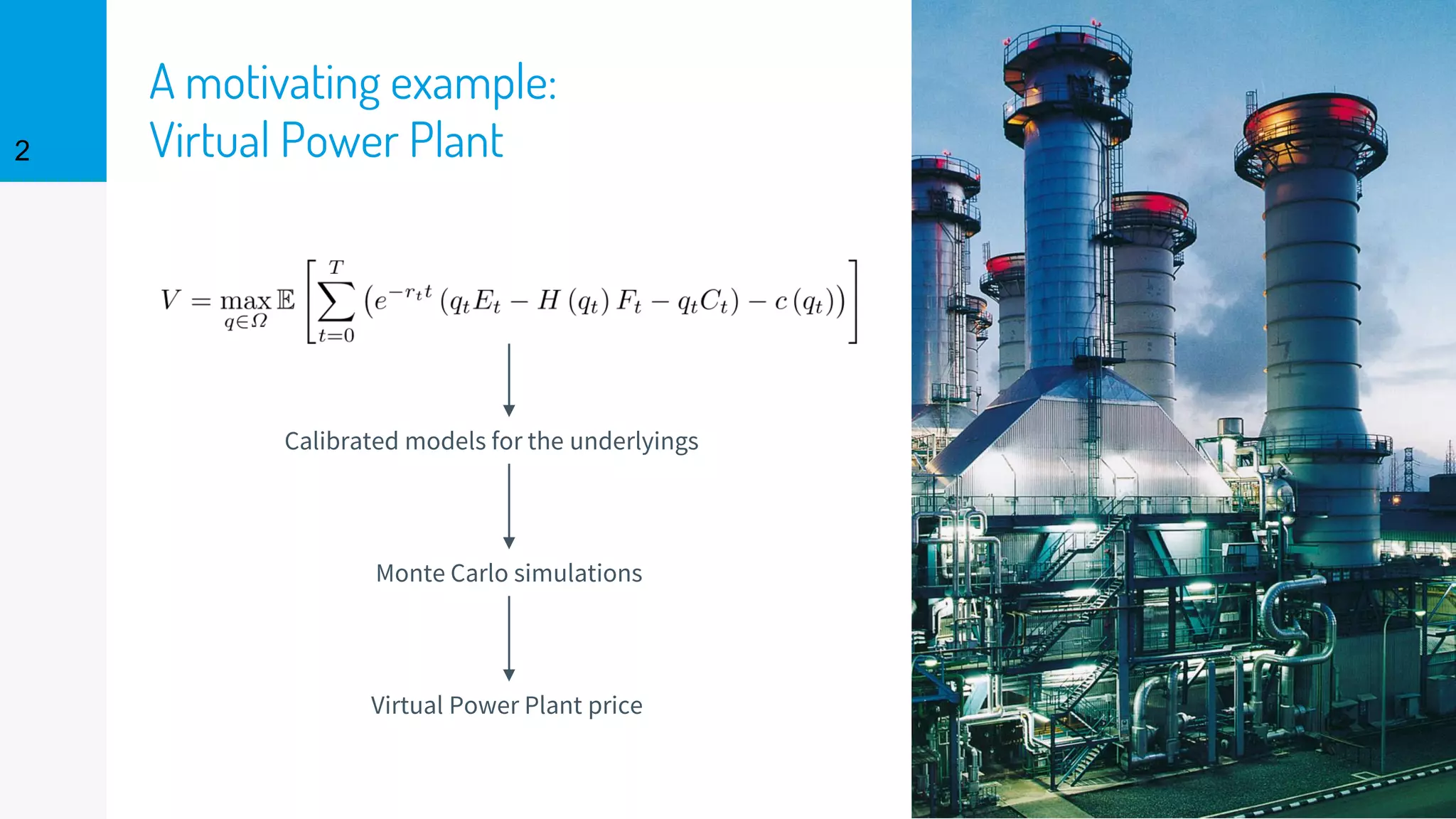
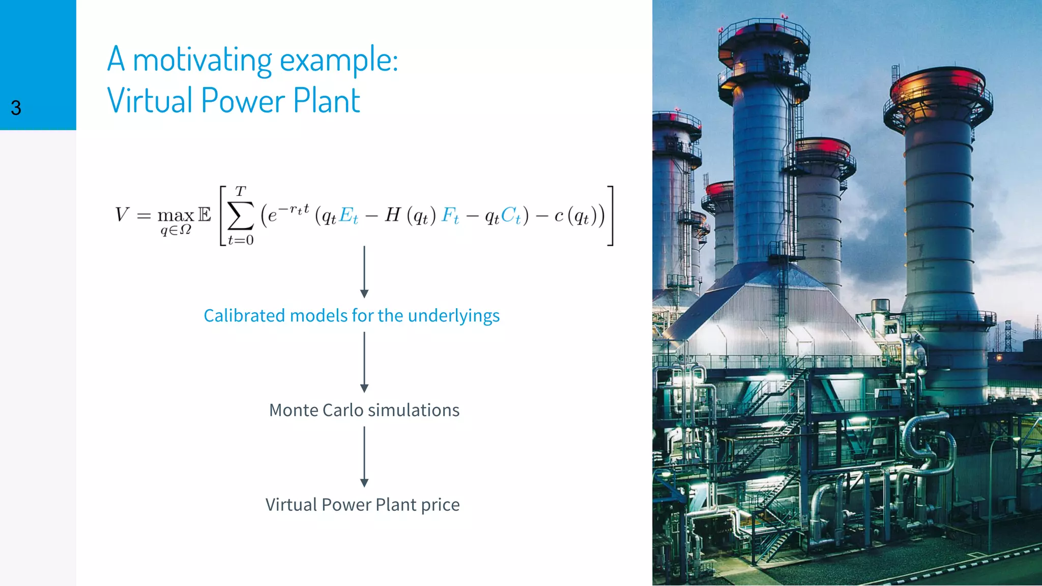

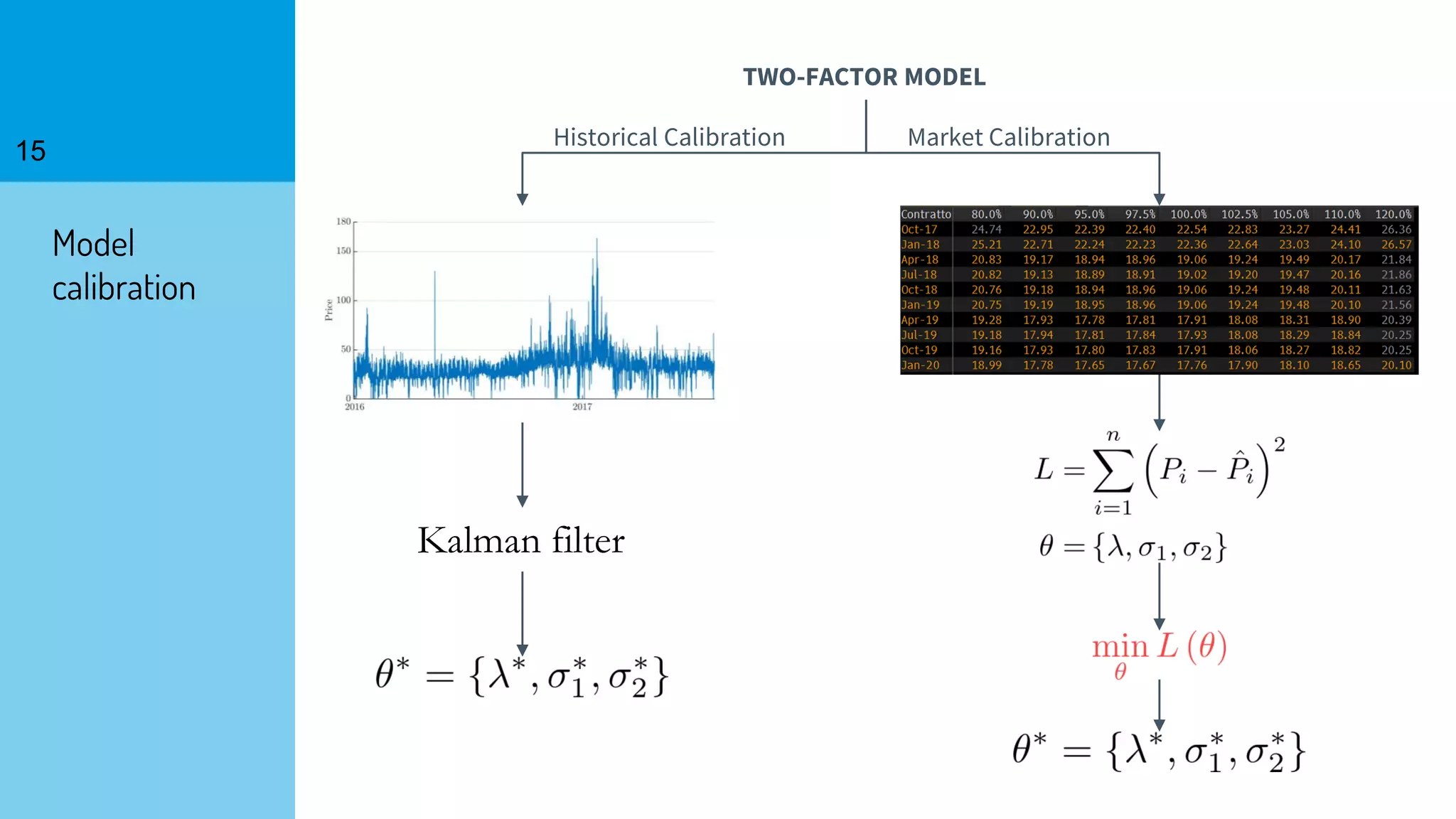
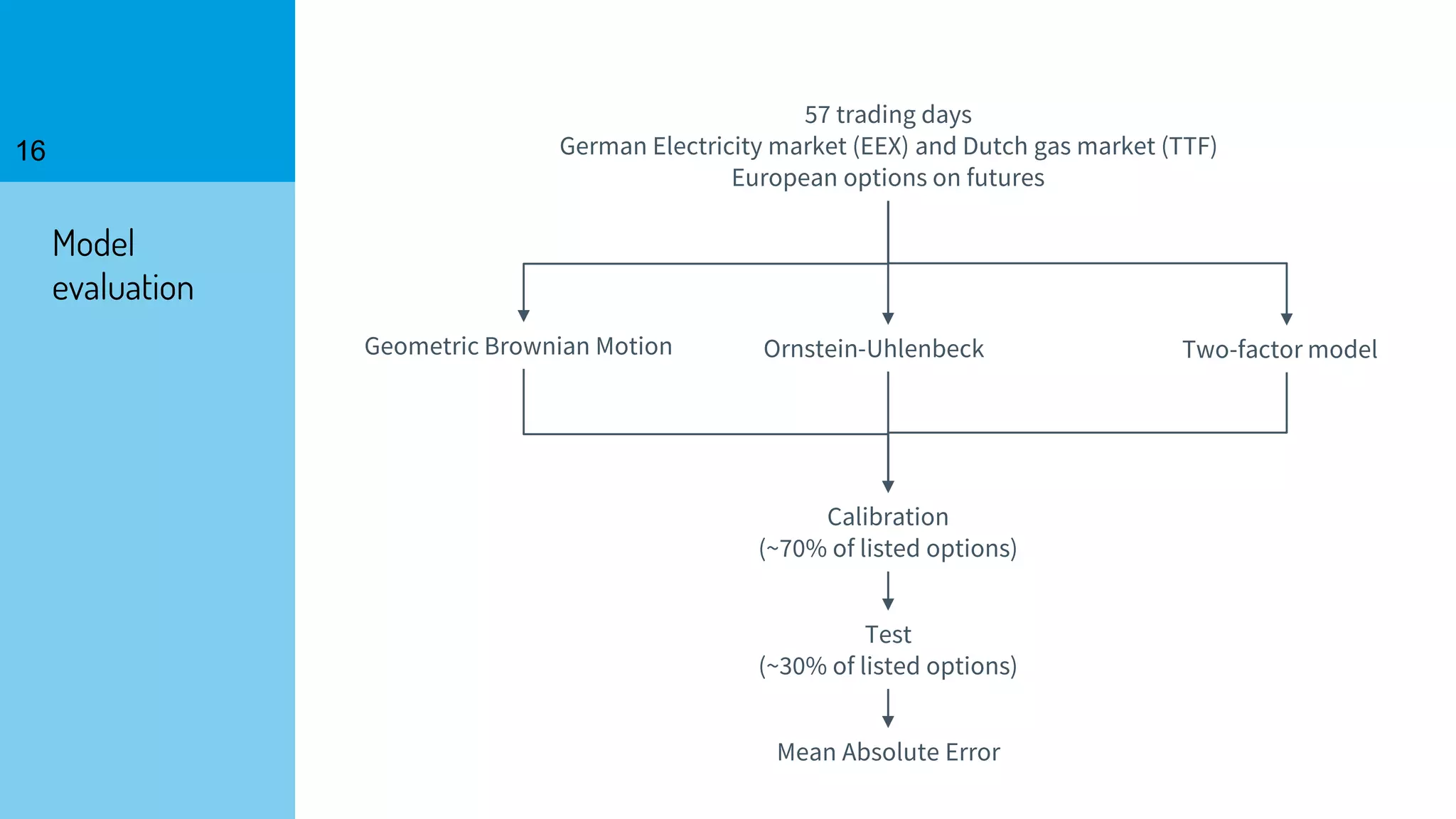
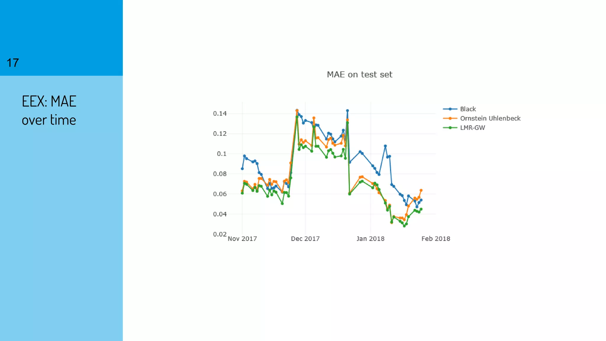
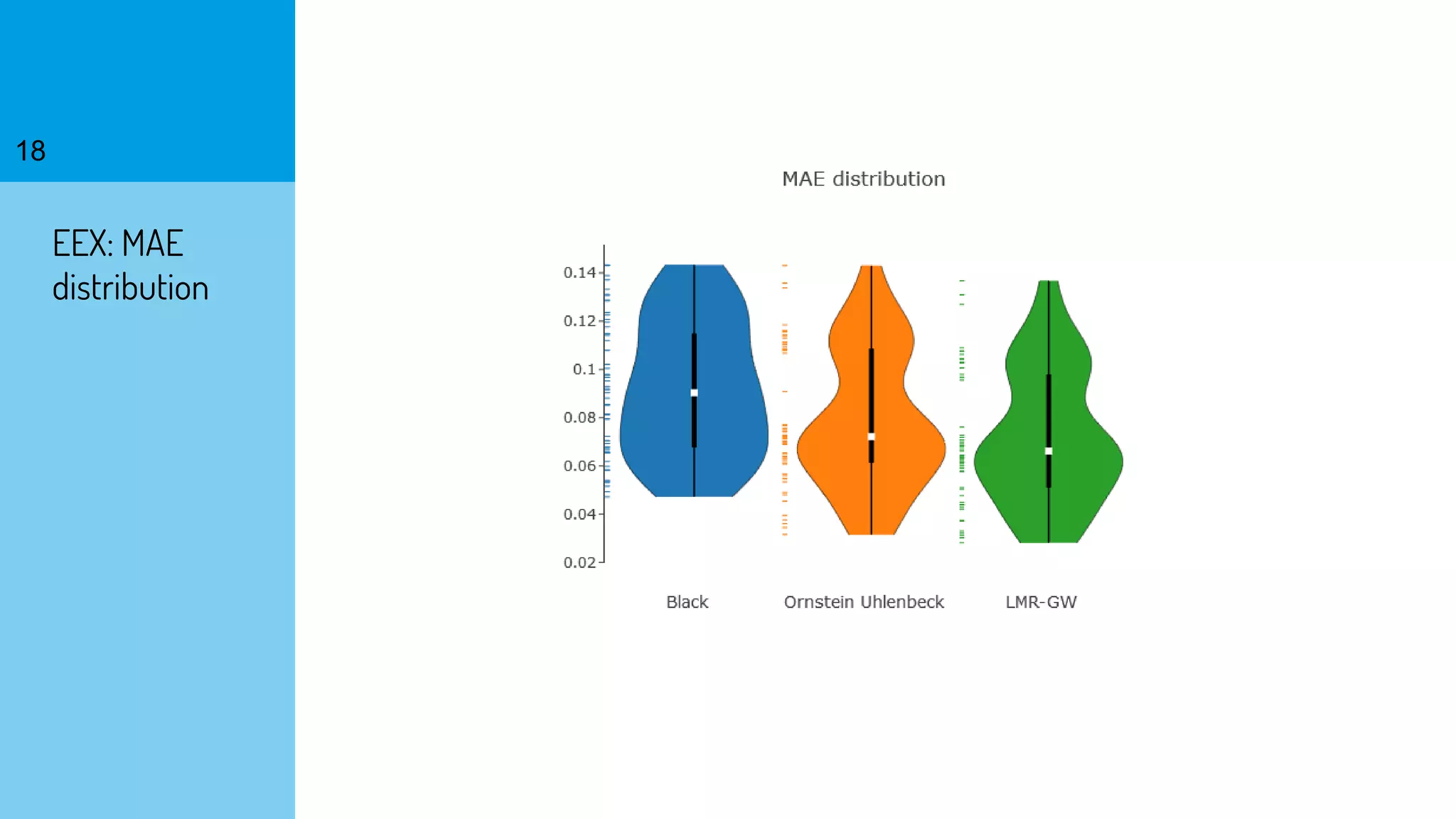
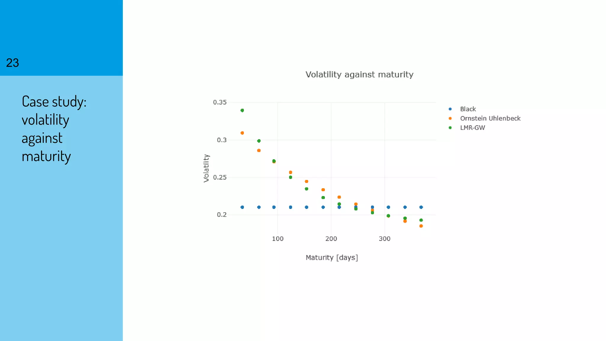
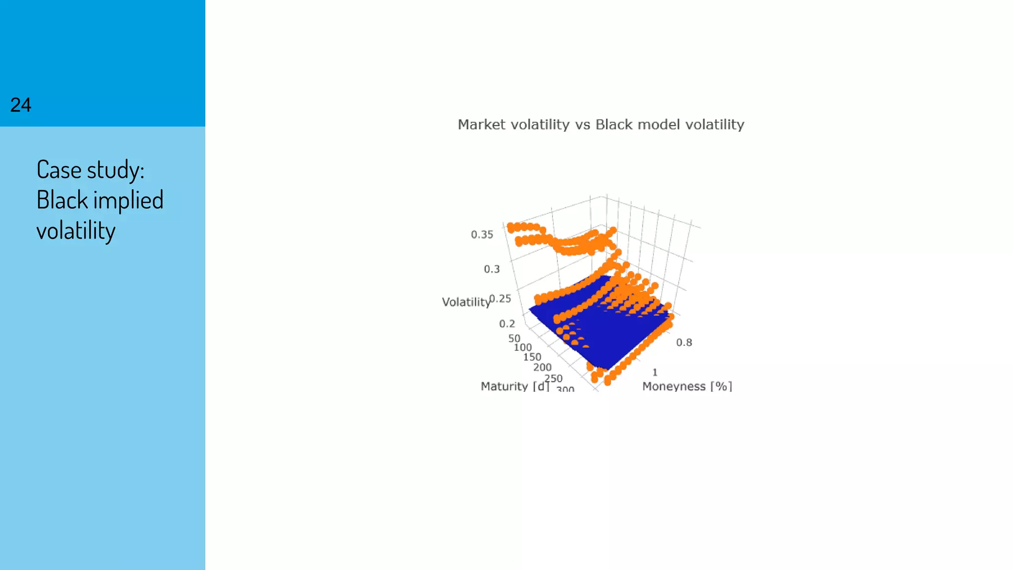
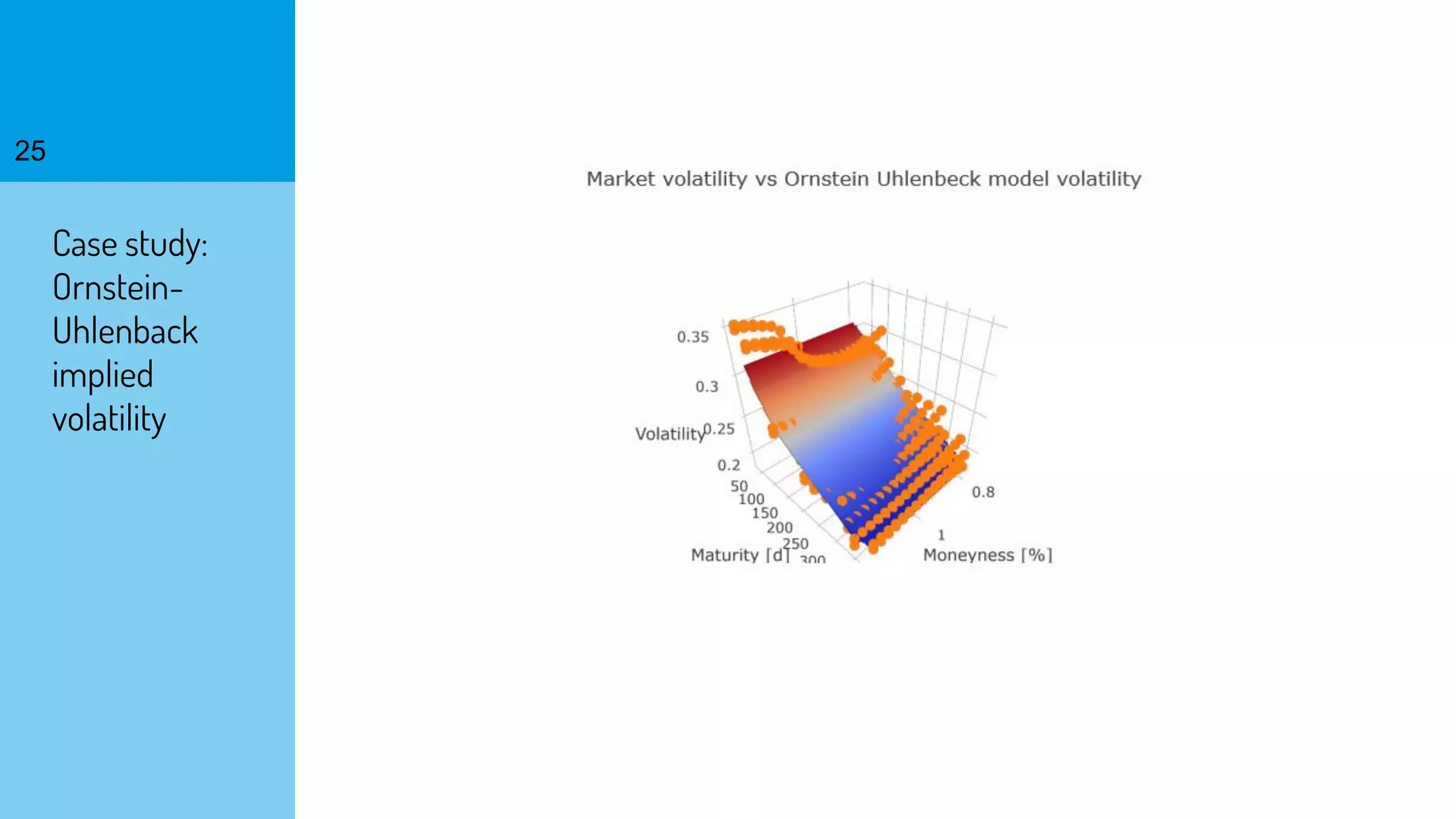
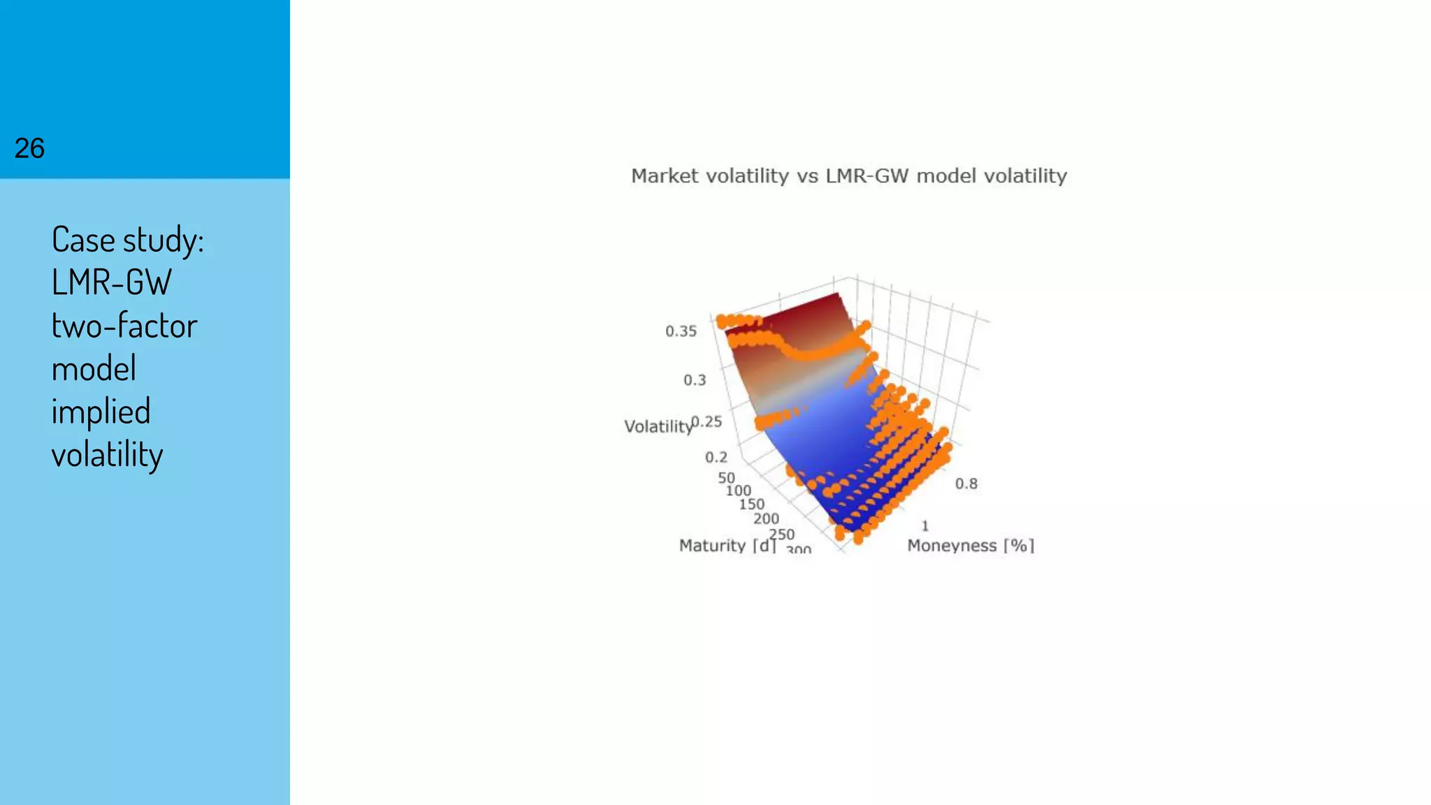


The document discusses the fast calibration of two-factor models for energy options pricing, particularly in relation to virtual power plants. It covers model choice, calibration methodologies, and evaluates models using historical data from the German electricity market and the Dutch gas market. Additionally, it highlights achievements in computational efficiency and suggests future developments such as testing new models and incorporating stochastic volatility.