Fake job predictor

1. Machine Learning Engineer Nanodegree
Capstone Project
Anshupriya Srivastava
January 26th, 2021
I. Definition
Project Overview
Employment scams are on the rise. According to CNBC, the number of employment scams doubled in
2018 as compared to 2017. The current market situation has led to high unemployment. Economic
stress and the impact of the coronavirus have significantly reduced job availability and the loss of jobs
for many individuals. A case like this presents an appropriate opportunity for scammers. Many people
are falling prey to these scammers using the desperation that is caused by an unprecedented incident.
Most scammer do this to get personal information from the person they are scamming. Personal
information can contain address, bank account details, social security number etc. I am a university
student, and I have received several such scam emails. The scammers provide users with a very lucrative
job opportunity and later ask for money in return. Or they require investment from the job seeker with
the promise of a job. This is a dangerous problem that can be addressed through Machine Learning
techniques and Natural Language Processing (NLP).
This project uses data provided from Kaggle. This data contains features that define a job posting. These
job postings are categorized as either real or fake. Fake job postings are a very small fraction of this
dataset. That is as excepted. We do not expect a lot of fake jobs postings. This project follows five
stages. The five stages adopted for this project are –
1. Problem Definition (Project Overview, Project statement and Metrics)
2. Data Collection
3. Data cleaning, exploring and pre-processing
4. Modeling
5. Evaluating
Figure 1. Stages of development
Problem Definition Data Collection
Data cleaning, exploring
and pre-processing
Modeling
Evaluation

2. Problem Statement
This project aims to create a classifier that will have the capability to identify fake and real jobs. The final result will
be evaluated based on two different models. Since the data provided has both numeric and text features one
model will be used on the text data and the other on numeric data. The final output will be a combination of the
two.
The final model will take in any relevant job posting data and produce a final result determining whether the job is
real or not.
Metrics
The models will be evaluated based on two metrics:
1. Accuracy: This metric is defined by this formula -
Accuracy=
True Positive+True Negative
True Positive+ False Positive+False Negative+True Negative
As the formula suggests, this metric produces a ratio of all correctly categorized data points to all data points. This
is particularly useful since we are trying to identify both real and fake jobs unlike a scenario where only one
category is important. There is however one drawback to this metric. Machine learning algorithms tend to favor
dominant classes. Since our classes are highly unbalanced a high accuracy would only be a representative of how
well our model is categorizing the negative class (real jobs).
2. F1-Score: F1 score is a measure of a model’s accuracy on a dataset. The formula for this metric is –
F1=
True Positive
True Positive+
1
2
(False Positive+False Negative)
F1-score is used because in this scenario both false negatives and false positives are crucial. This model needs to
identify both categories with the highest possible score since both have high costs associated to it.
II. Analysis
Data Exploration
The data for this project is available at Kaggle - https://www.kaggle.com/shivamb/real-or-fake-fake-jobposting-
prediction. The dataset consists of 17,880 observations and 18 features.
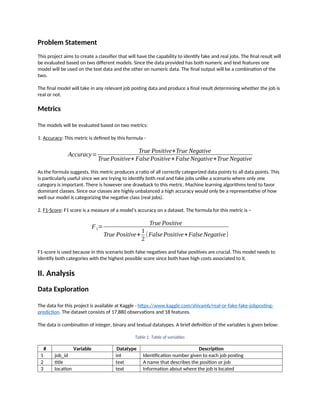
The data is combination of integer, binary and textual datatypes. A brief definition of the variables is given below:
Table 1. Table of variables
# Variable Datatype Description
1 job_id int Identification number given to each job posting
2 title text A name that describes the position or job
3 location text Information about where the job is located

3. 4 department text Information about the department this job is offered by
5 salary_range text Expected salary range
6 company_profile text Information about the company
7 description text A brief description about the position offered
8 requirements text Pre-requisites to qualify for the job
9 benefits text Benefits provided by the job
10 telecommuting boolean Is work from home or remote work allowed
11 has_company_logo boolean Does the job posting have a company logo
12 has_questions boolean Does the job posting have any questions
13 employment_type text 5 categories – Full-time, part-time, contract, temporary and
other
14 required_experience text Can be – Internship, Entry Level, Associate, Mid-senior level,
Director, Executive or Not Applicable
15 required_education text Can be – Bachelor’s degree, high school degree, unspecified,
associate degree, master’s degree, certification, some college
coursework, professional, some high school coursework,
vocational
16 Industry text The industry the job posting is relevant to
17 Function text The umbrella term to determining a job’s functionality
18 Fraudulent boolean The target variable  0: Real, 1: Fake
Since most of the datatypes are either Booleans or text a summary statistic is not needed here. The only integer is
job_id which is not relevant for this analysis. The dataset is further explored to identify null values.
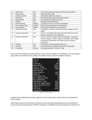
Figure 2. Missing values
Variables such as department and salary_range have a lot of missing values. These columns are dropped from
further analysis.
After initial assessment of the dataset, it could be seen that since these job postings have been extracted from
several countries the postings were in different languages. To simplify the process this project uses data from US

4. based locations that account for nearly 60% of the dataset. This was done to ensure all the data is in English for
easy interpretability.
Also, the location is split into state and city for further analysis. The final dataset has 10593 observations and 20
features.
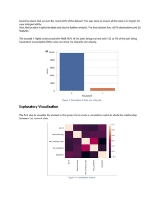
The dataset is highly unbalanced with 9868 (93% of the jobs) being real and only 725 or 7% of the jobs being
fraudulent. A countplot of the same can show the disparity very clearly.
Figure 3. Countplot of Real and fake jobs
Exploratory Visualization
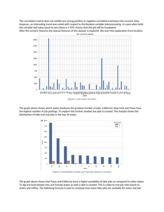
The first step to visualize the dataset in this project is to create a correlation matrix to study the relationship
between the numeric data.
Figure 4. Correlation matrix

5. The correlation matrix does not exhibit any strong positive or negative correlations between the numeric data.
However, an interesting trend was noted with respect to the Boolean variable telecommuting. In cases when both
this variable had value equal to zero there is a 92% chance that the job will be fraudulent.
After the numeric features the textual features of this dataset is explored. We start this exploration from location.
Figure 5. Job counts by states
The graph above shows which states produces the greatest number of jobs. California, New York and Texas have
the highest number of job postings. To explore this further another bar plot is created. This barplot shows the
distribution of fake and real jobs in the top 10 states.
Figure 6. Distribution of fake and real jobs based on location
The graph above shows that Texas and California have a higher possibility of fake jobs as compared to other states.
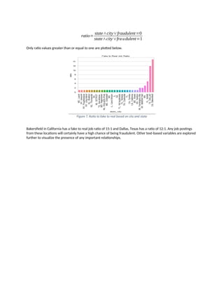
To dig one level deeper into and include states as well a ratio is created. This is a fake to real job ratio based on
states and citifies. The following formula is used to compute how many fake jobs are available for every real job:

6. ratio=
state∧city∨fraudulent=0
state∧city∨fra udulent=1
Only ratio values greater than or equal to one are plotted below.
Figure 7. Ratio to fake to real based on city and state
Bakersfield in California has a fake to real job ratio of 15:1 and Dallas, Texas has a ratio of 12:1. Any job postings
from these locations will certainly have a high chance of being fraudulent. Other text-based variables are explored
further to visualize the presence of any important relationships.

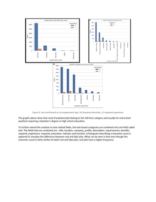
7. Figure 8. Job count based on (a) employment type, (b) Required education, (c) Required experience
The graphs above show that most fraudulent jobs belong to the full-time category and usually for entry-level
positions requiring a bachelor’s degree or high school education.
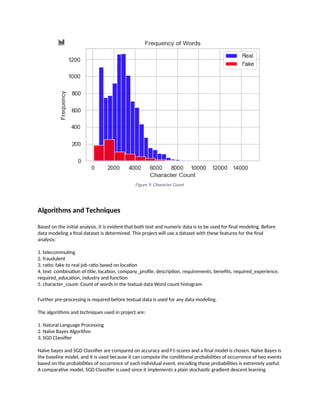
To further extend the analysis on text related fields, the text-based categories are combined into one field called
text. The fields that are combined are - title, location, company_profile, description, requirements, benefits,
required_experience, required_education, industry and function. A histogram describing a character count is
explored to visualize the difference between real and fake jobs. What can be seen is that even though the
character count is fairly similar for both real and fake jobs, real jobs have a higher frequency.

8. Figure 9. Character Count
Algorithms and Techniques
Based on the initial analysis, it is evident that both text and numeric data is to be used for final modeling. Before
data modeling a final dataset is determined. This project will use a dataset with these features for the final
analysis:
1. telecommuting
2. fraudulent
3. ratio: fake to real job ratio based on location
4. text: combination of title, location, company_profile, description, requirements, benefits, required_experience,
required_education, industry and function
5. character_count: Count of words in the textual data Word count histogram
Further pre-processing is required before textual data is used for any data modeling.
The algorithms and techniques used in project are:
1. Natural Language Processing
2. Naïve Bayes Algorithm
3. SGD Classifier
Naïve bayes and SGD Classifier are compared on accuracy and F1-scores and a final model is chosen. Naïve Bayes is
the baseline model, and it is used because it can compute the conditional probabilities of occurrence of two events
based on the probabilities of occurrence of each individual event, encoding those probabilities is extremely useful.
A comparative model, SGD Classifier is used since it implements a plain stochastic gradient descent learning

9. routine which supports different loss functions and penalties for classification. This classifier will need high
penalties when classified incorrectly. These models are used on both the text and numeric data separately and the
final results are combined.
Benchmark
The benchmark model for this project is Naïve bayes. The overall accuracy of this model is 0.971 and the F1-score
is 0.744. The reason behind using this model has been elaborated above. Any other model’s capabilities will be
compared to the results of Naïve bayes.
III. Methodology
Data Preprocessing
The following steps are taken for text processing:
Figure 10. Text Processing
 Tokenization: The textual data is split into smaller units. In this case the data is split into words.
 To Lower: The split words are converted to lowercase
 Stopword removal: Stopwords are words that do not add much meaning to sentences. For example: the,
a, an, he, have etc. These words are removed.
 Lemmatization: The process of lemmatization groups in which inflected forms of words are used together.
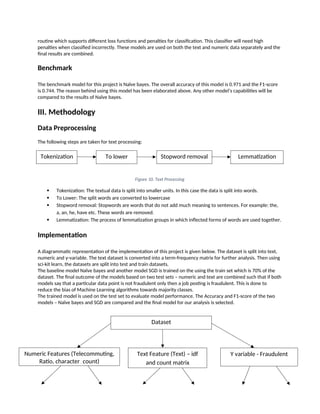
Implementation
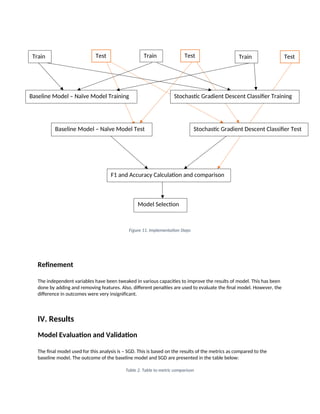
A diagrammatic representation of the implementation of this project is given below. The dataset is split into text,
numeric and y-variable. The text dataset is converted into a term-frequency matrix for further analysis. Then using
sci-kit learn, the datasets are split into test and train datasets.
The baseline model Naïve bayes and another model SGD is trained on the using the train set which is 70% of the
dataset. The final outcome of the models based on two test sets – numeric and text are combined such that if both
models say that a particular data point is not fraudulent only then a job posting is fraudulent. This is done to
reduce the bias of Machine Learning algorithms towards majority classes.
The trained model is used on the test set to evaluate model performance. The Accuracy and F1-score of the two
models – Naïve bayes and SGD are compared and the final model for our analysis is selected.
Tokenization To lower Stopword removal Lemmatization
Dataset
Numeric Features (Telecommuting,
Ratio, character_count)
Text Feature (Text) – idf
and count matrix
Y variable - Fraudulent

10. Figure 11. Implementation Steps
Refinement
The independent variables have been tweaked in various capacities to improve the results of model. This has been
done by adding and removing features. Also, different penalties are used to evaluate the final model. However, the
difference in outcomes were very insignificant.
IV. Results
Model Evaluation and Validation
The final model used for this analysis is – SGD. This is based on the results of the metrics as compared to the
baseline model. The outcome of the baseline model and SGD are presented in the table below:
Table 2. Table to metric comparison
Test Test Test
Train Train Train
Baseline Model – Naïve Model Training Stochastic Gradient Descent Classifier Training
Baseline Model – Naïve Model Test Stochastic Gradient Descent Classifier Test
F1 and Accuracy Calculation and comparison
Model Selection

11. Model Accuracy F1-score
Naïve Bayes (baseline model) 0.971 0.743
SGD 0.974 0.79
Based on these metrics, SGD has a slightly better performance than the baseline model. This is how the final model
is chosen to be SGD.
Justification
As mentioned above, the final model performs better than the established benchmark of the baseline model. The
model will be able to identify real jobs with a very high accuracy. However, it’s identification of fake jobs can still
be improved upon.
V. Conclusion
Free-Form Visualization
A confusion matrix can be used to evaluate the quality of the project. The project aims to identify real and fake
jobs.
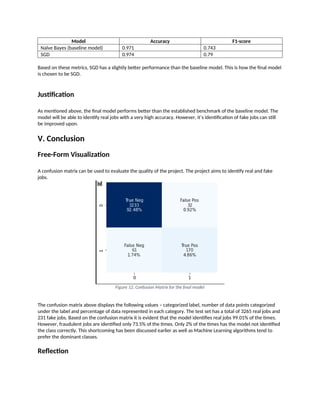
Figure 12. Confusion Matrix for the final model
The confusion matrix above displays the following values – categorized label, number of data points categorized
under the label and percentage of data represented in each category. The test set has a total of 3265 real jobs and
231 fake jobs. Based on the confusion matrix it is evident that the model identifies real jobs 99.01% of the times.
However, fraudulent jobs are identified only 73.5% of the times. Only 2% of the times has the model not identified
the class correctly. This shortcoming has been discussed earlier as well as Machine Learning algorithms tend to
prefer the dominant classes.
Reflection

12. Fake job postings are an important real-world challenge that require active solutions. This project aims to provide a
potential solution to this problem. The textual data is pre-processed to generate optimal results and relevant
numerical fields are chose as well. The output of Multiple models is combined to produce the best possible results.
This is done to reduce the bias that a machine learning model has towards the dominant class.
The most interesting part of this project was how certain locations are an epitome of fraudulent jobs. For example,
Bakersfield, California has a fake to real job ratio of 15:1. Places like this require some extra monitoring. Another
interesting part was that most entry level jobs seem to be fraudulent. It seems like scammers tend to target
younger people who have a bachelor’s degree or high school diploma looking for full-time jobs.
The most challenging part was text data preprocessing. The data was in a very format. Cleaning it required a lot of
effort.
Improvement
The dataset that is used in this project is very unbalanced. Most jobs are real, and few are fraudulent. Due to this,
real jobs are being identified quite well. Certain techniques like SMOTE can be used to generate synthetic minority
class samples. A balanced dataset should be able to generate better results.