Exposureresponse Modeling Methods And Practical Implementation 1st Edition Jixian Wang
Exposureresponse Modeling Methods And Practical Implementation 1st Edition Jixian Wang
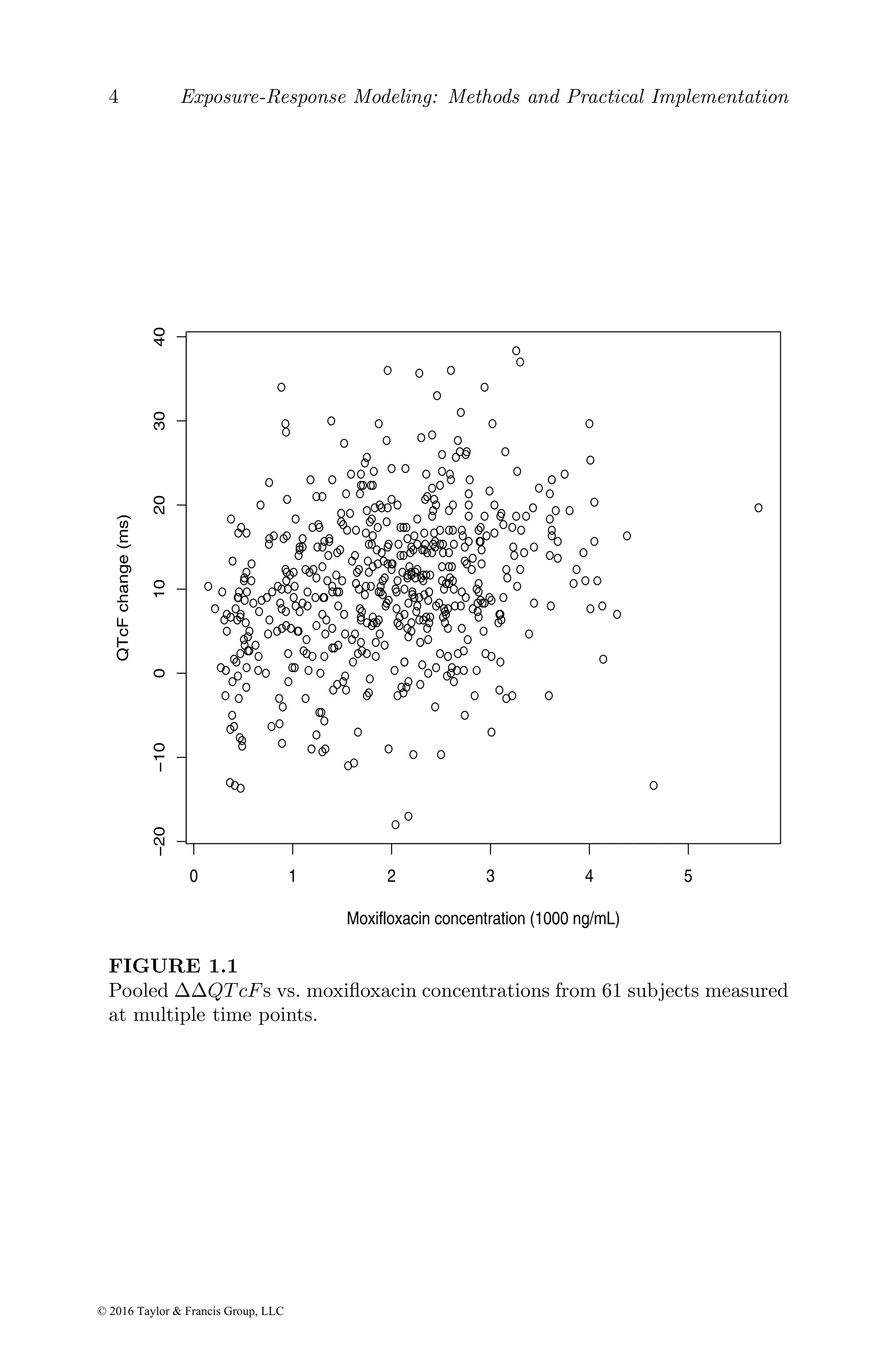
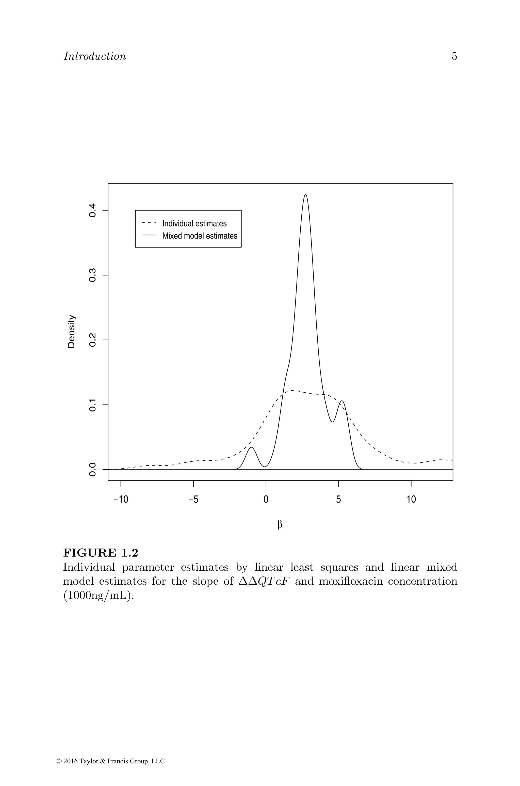
Exposureresponse Modeling Methods And Practical Implementation 1st Edition Jixian Wang


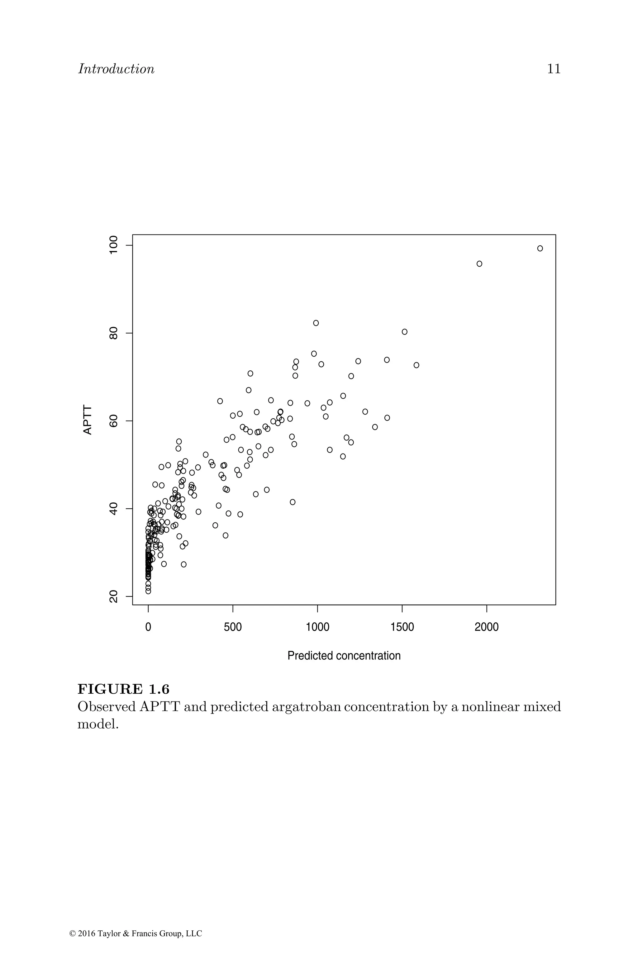
![Basic exposure and exposure–response models 25
approach (TBS, Carroll and Ruppert, 1988). Typically a log TBS is a bridge
between additive and multiplicative models. One reason for using a transfor-
mation from a statistical aspect is to make the distribution of the response
easy to handle with a simple model. The log-transformation is the most com-
mon one to use. The transformation also converts a multiplicative model to
an additive one, and the latter is often much easier to fit. Some transforma-
tions proposed from purely statistical aspects, particularly those depending
on extra-parameters, such as the Box–Cox transformation, are used less fre-
quently than the log-transformation in ER modeling. Here we will mainly
focus on the log-transformation.
Consider the theophylline concentration data. Since there is no dosing
history data, we model the concentration data before any dose adjustment is
made. Let ci be the concentration from patient i at 0.01 h. We fitted a linear
model for log-transformed ci and covariates:
log(ci) = XT
i β + ei, (2.19)
where ei ∼ N(0, σ2
e). Note that this model might be considered as an approx-
imation to model (2.6). The data were fitted by the linear regression function
lm(.) in R. After fitting models with different combinations of covariates in
Xi, we found that only age is related to ci (denoted as THEO in the outputs)
and the fitted model is
lm(formula = log(THEO) ~ log(AGE), data = short[short$TIME ==0.01, ])
Coefficients:
Estimate Std. Error t value Pr(>|t|)
(Intercept) -0.8623 0.9418 -0.916 0.3618
log(AGE) 0.5699 0.2655 2.147 0.0339
The other factors included in the dataset might have been sufficiently adjusted
when planning the initial dose. Transforming back to the original scale, we get
the geometric mean of ci as
exp(XT
i β̂) = exp(−0.862)AGE0.570
(2.20)
which is in the form of the power model. The key feature is that the contri-
butions of the factors are multiplicative to each other. Note that Eg
(yi) =
exp(XT
i β) is the geometric mean of yi and E(yi) = exp(XT
i β)E(exp(ei)) >
exp(XT
i β). Geometric means are commonly used for modeling exposure data,
but may not always be appropriate for PKPD modeling.
Transformations are also used for nonlinear models. The error structure of
the model is a key factor to consider for selecting an appropriate transforma-
tion. We take the Emax model (2.3) as an example to show how to select the
transformation. Suppose that yi is positive (e.g., the tumor size or a positive
valued biomarker) and its relationship with ci has a sigmoid-like shape; then
the following model may be considered:
log(yi) = log(Emax/(1 + EC50/ci)εi)
= log(Emax) − log(1 + EC50/ci) + log(εi) (2.21)
© 2016 Taylor & Francis Group, LLC](https://image.slidesharecdn.com/2645101-250722182738-ee90be60/75/Exposureresponse-Modeling-Methods-And-Practical-Implementation-1st-Edition-Jixian-Wang-47-2048.jpg)
![28 Exposure-Response Modeling: Methods and Practical Implementation
those with knots at 0 and 1 only (known as boundary knots). In this case,
the B-splines are terms of Ck
nxn
(1 − x)k
, k = 0, ..., n, with Ck
n the number of
combinations of taking k balls from a total of n. With only boundary knots,
the cubic B-spline has n = 3 + 1 = 4 such terms. Using function bs() in R
library splines, we can construct
> x=(0:10)/10
> cbind(x,bs(x,degree = 3,intercept=T))
x 1 2 3 4
[1,] 0.0 1.000 0.000 0.000 0.000
[2,] 0.1 0.729 0.243 0.027 0.001
[3,] 0.2 0.512 0.384 0.096 0.008
[4,] 0.3 0.343 0.441 0.189 0.027
[5,] 0.4 0.216 0.432 0.288 0.064
[6,] 0.5 0.125 0.375 0.375 0.125
[7,] 0.6 0.064 0.288 0.432 0.216
[8,] 0.7 0.027 0.189 0.441 0.343
[9,] 0.8 0.008 0.096 0.384 0.512
[10,] 0.9 0.001 0.027 0.243 0.729
[11,] 1.0 0.000 0.000 0.000 1.000
gives the function values at different x. With one interior knot at 0.5, there is
one more term
> bs(x,degree = 3,knots=0.5,intercept=T)
1 2 3 4 5
[1,] 1.000 0.000 0.000 0.000 0.000
[2,] 0.512 0.434 0.052 0.002 0.000
[3,] 0.216 0.592 0.176 0.016 0.000
[4,] 0.064 0.558 0.324 0.054 0.000
[5,] 0.008 0.416 0.448 0.128 0.000
[6,] 0.000 0.250 0.500 0.250 0.000
[7,] 0.000 0.128 0.448 0.416 0.008
[8,] 0.000 0.054 0.324 0.558 0.064
[9,] 0.000 0.016 0.176 0.592 0.216
[10,] 0.000 0.002 0.052 0.434 0.512
[11,] 0.000 0.000 0.000 0.000 1.000
attr(,"degree")
[1] 3
attr(,"knots")
[1] 0.5
attr(,"Boundary.knots")
[1] 0 1
However, one of the terms is redundant as it is a linear combination of the
others. This can be seen from that Ck
nxn
(1−x)k
s are the probability of having
k events in n trials when x is the probability, hence
Pn
k=1 Ck
nxn
(1 − x)k
= 1.
Therefore, to fit B-splines to, e.g.,
√
x, one should use the bs() function without
the option intercept= T , which is the default, of not produce the first term:
© 2016 Taylor & Francis Group, LLC](https://image.slidesharecdn.com/2645101-250722182738-ee90be60/75/Exposureresponse-Modeling-Methods-And-Practical-Implementation-1st-Edition-Jixian-Wang-50-2048.jpg)
![30 Exposure-Response Modeling: Methods and Practical Implementation
which gives
lm(formula = log(resp) ~ log(base) + bs(pred, 3), data = data240)
Coefficients:
(Intercept) log(base) bs(pred, 3)1 bs(pred, 3)2 bs(pred, 3)3
1.2619 0.7671 0.3914 0.3924 0.7522
The coefficients for the spline functions are difficult to interpret directly. But
since the B-spline functions are basis functions between the knots, an increas-
ing trend of the coefficient indicates the same trend in the exposure–response
relationship. This can also be seen from the previous B-spline examples in
(0,1).
In a semiparametric model, it could be that the nonparametric or the
parametric part is of the primary interest. For example, to explore the dose-
response relationship in argatroban data, one may fit a model with spline
functions for the time profile using dose as the covariate. Since this analysis
involves repeated measurements and needs a linear mixed model, it will be
postponed until the next chapter.
Semiparametric methods can also be used to extend GLMs by using a
smoothing method on the linear predictor. For example, one can add spline
functions for exposure to a GLM model and obtain
g(E(yi)) = XT
i β +
K
X
k=1
Bk(ci)ηk. (2.29)
This type of model is known as a generalized additive model, as the spline
function part is additive in the linear predictor. We have seen a large difference
between the fitted logistic models with and without placebo data, indicating
that the data present a more complex ER relationship than a linear model can
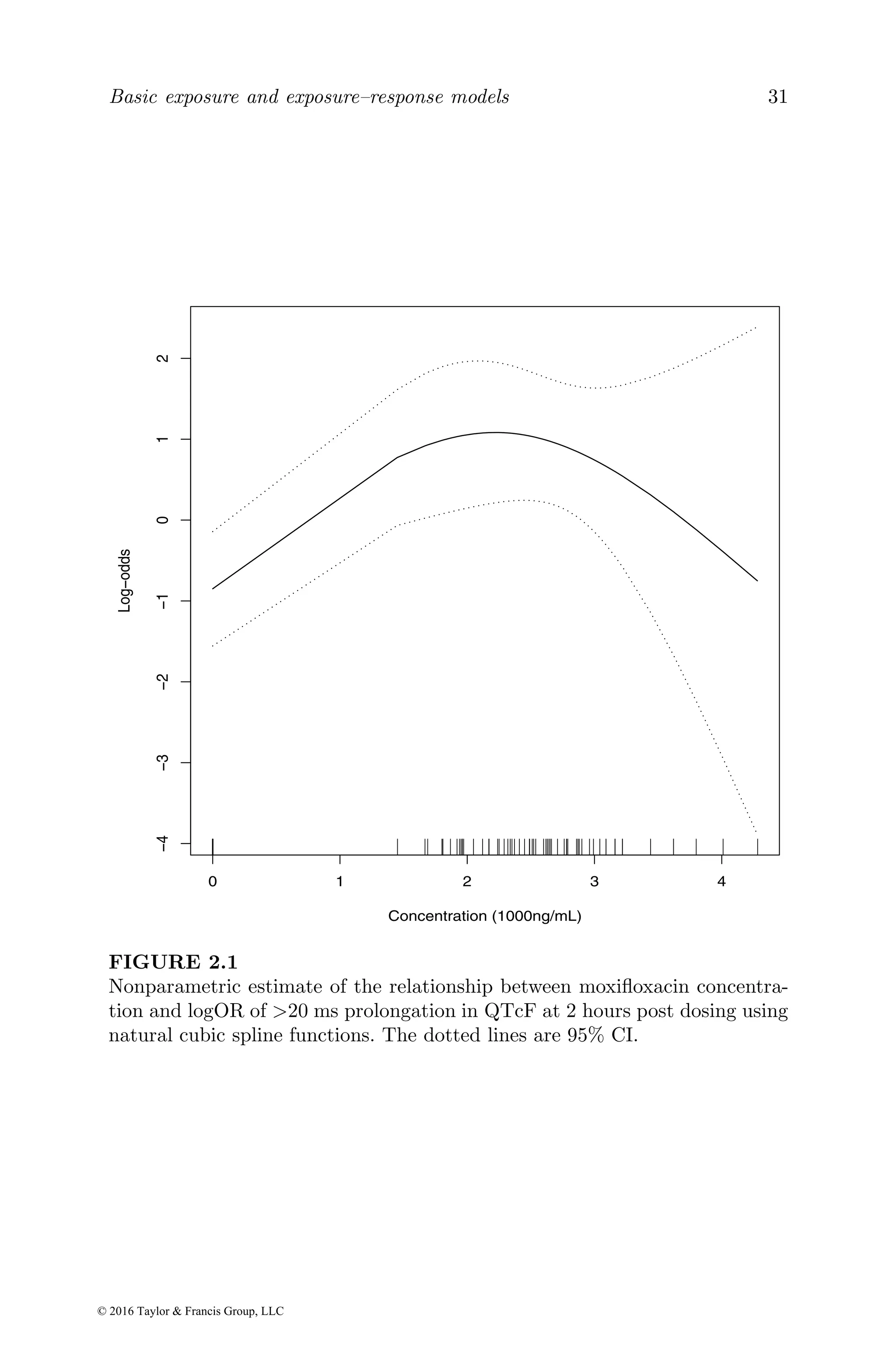
describe. Fitting a logistic model with natural cubic spline functions using
fit=gam(qtp~ns(conc,3),family=binomial,data=moxi[moxi$time==2,])
where qtq and conc are the moxifloxacin concentration and response, respec-
tively, at 2 hours, gives a bell-shaped curve for the relationship between the
concentration and logOR (Figure 2.1). The results indicate a nonlinear rela-
tionship between moxifloxacin exposure and QT prolongation globally. The
model fitted to all the data was driven by the strong impact of the risk in-
crease from zero to low concentration, while that fitted to the moxifloxacin
data was affected by the right end of the curve and resulted in a negative lo-
gOR. The lower and higher ends of the curve are very uncertain, as there was
no event between concentration ranges of zero and 1870 ng/mL and higher
than 3000 ng/mL. Although there is an initial increase in the risk along with
the exposure increase, the left part of the curve cannot be quantified. There
is no evidence of an ER relationship in the higher concentration range. In
summary, there is not sufficient information to quantify the overall ER rela-
tionship based on the parametric and semiparametric models. We will show
© 2016 Taylor & Francis Group, LLC](https://image.slidesharecdn.com/2645101-250722182738-ee90be60/75/Exposureresponse-Modeling-Methods-And-Practical-Implementation-1st-Edition-Jixian-Wang-52-2048.jpg)