The document outlines an Excel project for creating a workbook with four worksheets focusing on car rental revenue analysis for a rental car company. The project requires various Excel functionalities including pivot tables, charts, and written analysis based on provided data. The guidelines specify formatting, data handling, and analysis tasks aimed at generating insights from the rental revenue data.

1. Excel Project 2 – MS Excel
Summer 2018
Use the project description HERE to complete this activity. For
a review of the complete rubric used in grading
this exercise, click on the Assignments tab, then on the title
Excel Project #2. Click on Show Rubrics if the
rubric is not already displayed.
Summary
Create a Microsoft Excel workbook with four worksheets that
provides extensive use of Excel capabilities
including creating a pivot table, charting, and written analysis
and recommendations in support of a business
enterprise.
A large rental car company has two metropolitan locations, one
at the airport and another centrally located in
downtown. It has been operating since 2015 and each location
summarizes its car rental revenue
quarterly. Both locations rent two classes of cars: economy and
premium. Rental revenue is maintained
separately for the two classes of rental vehicles.
The data for this case resides in the file
summer2018rentalcars.txt and can be downloaded by clicking
on the
Assignments tab, then on the data file name. It is a text file
with the file type .txt.

2. Do not create your own data. You must use the data provided,
and only the data provided.
Default Formatting: All labels, text, and numbers will be Arial
10, There will be $ and comma and
decimal point variations for numeric data, but Arial 10 will be
the default font and font size.
Tutorials
Note: Tutorials that address activities used in this project have
been assigned in Week 1 – 5.
Step Requirement
Points
Allocated
Comments
1
Open Excel and save a blank workbook with the following
name:
a. “Student’s First InitialLast Name Excel Project 2”
Example: JSmith Excel Project 2.
b. Set Page Layout Orientation to Landscape.
0.2
Use Print Preview to review
how the first worksheet

3. would print.
2 Change the name of the worksheet to Analysis by. 0.1
3
In the Analysis by worksheet:
a. Beginning in Row 1, enter the four labels in column
A (one label per row) in the following order:
Name:, Class/Section:, Project:, Date Due:
b. Place a blank row between each label. Please note
the colon : after each label.
c. Align the labels to the right side in the cells
It may be necessary to adjust the column width so the four
labels are clearly visible.
0.3
Format for text in column
A:
• Arial 10 point
• Normal font
• Right-align all four
labels in the cells

4. 4
In the Analysis by worksheet with all entries in column C:
a. Enter the appropriate values for your Name, Class
and Section, Project, Date Due across from the
appropriate label in column A.
0.2
Format for text in column
C:
• Arial 10 point
• Bold
Step Requirement
Points
Allocated
Comments
b. Use the formatting in the Comments column (to the
right).
It may be necessary to adjust the column width so the four
labels are clearly visible.
• Left-align all four
values in the cells

5. 5
a. Create new worksheets:
Data, Initial Analysis, Profit Analysis.
Upon completion, there should be Analysis by as
well as the three newly created worksheets.
b. Delete any other worksheets.
Note: The three new worksheets might not have Arial 10
point as the default type so it may be necessary to change
the font and point to Arial 10 for each worksheet.
If necessary, reorder the four worksheets so they are in the
following order: Analysis by, Data, Initial Analysis, Profit
Analysis.
0.2
6
After clicking on the blank cell A1 (to select it) in the Data
worksheet:
a. Import the text file summer2018rentalcars.txt into
the Data worksheet.
b. Adjust all column widths so there is no data or
column header truncation.
Though the intent is to import the text file into the Data
worksheet, sometimes when text data is imported into a
worksheet, a new worksheet is created. If this happens,
delete the blank Data worksheet, and then rename the new

6. worksheet which HAS the recently imported data as “Data.”
It may be necessary to change Revenue data to Currency
format ($ and comma (thousands separators)) with NO
decimal points, and to change NumCars data to Number
format with NO decimal points, but with the comma
(thousands separator) because of the import operation.
This may or may not occur, but in case it does it needs to
be corrected.
0.2
Format for all data
All data (field names, data
text, and data numbers)
• Arial 10 point.
• Normal font
The field names should be
in the top row of the
worksheet with the data
directly under it in rows.
This action may not be
necessary as this is part of
the Excel table creation
process. The data should
begin in Column A.
7

7. In the Data worksheet:
a. Create an Excel table with the recently imported
data.
b. Pick a style with the styles group to format the table
(choose a style that shows banded rows, i.e., rows
that alternate between 2 colors).
c. The style should highlight the field names in the first
row. These are your table headers.
d. Ensure NO blank cells are part of the specified data
range.
e. Ensure that Header Row and Banded Rows are
selected in the Table Style Options Group Box. Do
NOT check the Total Row.
0.5
Some adjustment may be
necessary to column widths
to ensure all field names
and all data are readable
(not truncated or
obscured).
Step Requirement
Points

8. Allocated
Comments
8
In the Data worksheet:
a. Sort the entire table by Year (ascending)
b. Delete all 2017 data. There should be one row for
titles and thirty-two rows of data after the 2017 data
is deleted.
c. There should be no column or data truncation.
0.3
9
Copy the entire table on the Data worksheet (column
headings and data) to the Initial Analysis worksheet.
a. Ensure that all field names as well as the data is
readable
b. Ensure that Revenue data is in Currency format ($
and comma (thousands separators)) with NO
decimal points, and NumCars data is in Number
format with NO decimal points, but with the comma
(thousands separator).
c. The upper left hand corner of the table should be in
cell A1 of the Initial Analysis worksheet
0.3

9. Format
for all data, text and labels
and numerical content:
• Arial 10
• Normal font.
10
In the Initial Analysis worksheet, using the table just
copied there:
a. Create a Pivot Table.
b. Adjust column widths if necessary to eliminate title
and data truncation.
c. Locate the top edge of the Pivot Table in at the top
edge of Row 1 and a few columns to the right of the
data
In the Pivot Table:
d. Display the total revenue for Economy as well as
Premium class cars.
e. Display the total revenue for both Airport and
Downtown locations.
f. Row and column calculations (sum) are required so

10. that the total revenue for EACH location and the
total revenue for EACH carclass are visible in the
pivot table. There must be a grand total that
represents the sum of ALL revenue.
g. Ensure that the formatting is as listed in the
Comments column.
0.7
There should be no 2017
data on the Initial Analysis
worksheet.
Format (for all data):
• Currency (leading dollar
sign)
• No decimal places
• Arial 10 point
• Normal font
Note: Formatting is for
the data copied to this
worksheet AND for the
created pivot table.
11
In the Initial Analysis worksheet:
a. Create a column or bar type of chart that shows the

11. total revenue for both vehicle types at each
location.
b. Add a title that reflects the information presented by
the chart.
c. The upper left corner of the chart should be one or
two rows below the above referenced pivot table
and left aligned with the pivot table.
d. Ensure the location and type of car is clearly
indicated in the chart.
0.7
The chart should allow a
viewer to determine
approximate revenue totals
for each vehicle total
revenue at each location.
The chart should have no
more than 4 bars or
columns.
Step Requirement
Points
Allocated
Comments

12. For the question below, present your answers in a very readable
format. These answers should be placed on
the page below the chart and table, if there is sufficient room on
that page. Do not let the answers be "split"
over more than one page. You can type your answer in one cell
(in Column A), then highlighting and selecting
several rows and columns, selecting merge cells and selecting
Wrap Text. Do NOT widen the columns as this
will adversely impact the appearance of the pivot tables above.
You will want to change the text from Center
to Left justification. Play with this a bit. If you simply type
your answer on a single line in Column A, that will
also be ok. But be sure the entire answer can be read without
the reader having to change any
formatting or view the results in the cell contents box.
12
Question 1: Based on the Initial Analysis worksheet,
which location for 2015 and 2016 combined produced the
most revenue? How much revenue was it?
a. Label your response Question 1. Answer this
question in 2 to 3 sentences. (0.3)
b. Readability, format and location (0.2)
c. No errors in grammar or spelling (0.1)
0.6
Use the following text

13. format:
• Arial 10 point
• Normal/Black
• Left-align text in the cell
13
Copy the entire table (column headings and data) from the
Data worksheet to the Profit Analysis worksheet.
a. In the Profit Analysis worksheet the field names
should be in Row 1 and the Year column should be
in column A.
b. Ensure that Revenue data is in Currency format ($
and comma (thousands separators)) with NO
decimal points, and NumCars data is in Number
format with NO decimal points, but with the comma
(thousands separator).
Some column adjustments may be necessary to ensure the
field names as well as the data is all readable.
0.2
Format
for all data, text and labels
and numerical content:

14. • Arial 10
• Normal font.
14
In the Profit Analysis worksheet:
In the column to the immediate right of NumCars label,
a. Create a label called Overhead.
b. Adjust the newly created column width, if
necessary.
0.2
Format:
• Arial 10 point
• Normal font
15
Overhead costs include maintenance, cleaning, and
administrative expenses associated with a car rental. The
Overhead for one rental transaction is $50 for an economy
car and $75 for a premium car. This Overhead cost
includes maintenance, cleaning, and administrative costs
for each car rental.
a. With this information, in the Profit Analysis
worksheet, in the first cell under the Overhead
label, calculate the overhead that corresponds to
the number of cars rented (NumCars) using an "IF"

15. statement as part of the formula.
b. For clarification, use the "IF" statement to determine
whether to use $50 or $75 times the NumCars so
that the Overhead value represents the total
Overhead costs for the Number of Cars (NumCars)
rented in a given row.
1.0
No credit if an IF
statement is NOT used.
Format:
• Currency with no
decimal points.
• Arial 10 point
• Normal/Black
• Right-align values
in the cell
Step Requirement
Points
Allocated
Comments
No credit if an IF statement is NOT used.

16. 16
In the Profit Analysis worksheet:
a. Copy the overhead formula to all the cells below in
the Overhead column. Adjust the column width if
necessary for legibility.
b. Ensure overhead data format is Currency ($ and
using comma as thousands separators) with NO
decimal points.
Note: Each row in the new column must have the same
general appearance (color, shading) as the other cells to its
left in that same column.
0.2
No credit if an IF
statement is NOT used.
Format:
• Currency with no
decimal points.
• Arial 10 point
• Normal/Black
• Right-align values in the
cell

17. 17
In the Profit Analysis worksheet:
In the next column to the right of the Overhead label,
a. Create a label called Profit.
0.1
Format:
• Arial 10 point
18
In the Profit Analysis worksheet, profit represents the
difference between Revenue and Overhead (Revenue –
(minus) Overhead) for the data IN the same row as the
profit data shown. Profit is for all cars rented during the
quarter.
In the first cell below the label Profit:
a. Calculate the profit,
b. Then copy the formula for all cells in that column (if
necessary).
c. Adjust the column width if necessary for legibility.

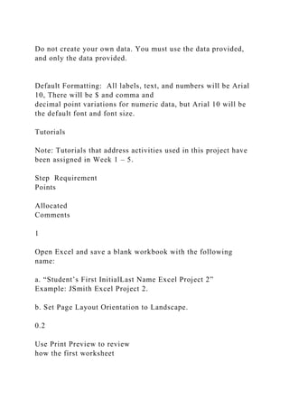
18. Note: If you are clicking on cells to construct a formula, you
may see [@Revenue]-[@Overhead in the cell editor, a
result of using an Excel table. One can create a formula by
typing the cell location instead of clicking on a particular
cell. In Excel, there are often many different ways to
accomplish the same task. Double-checking the
calculation with a hand-held calculator can identify possible
errors.
Note: Each row in the new column must have the same
general appearance (color, shading) as the other cells to its
left in that same column.
0.3
Format:
• Currency ($ and
comma as thousands
separators) with no
decimal points.
• Arial 10 point
• Normal/Black
• Right-align values in the
cell
19

19. In the Profit Analysis worksheet, in the next column to the
right of the label Profit,
a. Create a label called Profit per Car.
b. Adjust the column width if necessary for legibility.
0.2
Format:
• Arial 10 point
• Normal font
20
In the Profit Analysis worksheet, in the next cell down
under the Profit per Car label:
a. Calculate the profit per car rented. Profit per Car
reflects the data in that particular row.
0.3
Format:
• Currency ($) with TWO
decimal points.
• Arial 10 point
• Normal

20. Step Requirement
Points
Allocated
Comments
b. Copy the formula to all cells below. Double-
checking the calculation with a hand-held calculator
can identify possible errors.
c. Adjust the column width if necessary for legibility.
Note: Each row in the new column must have the same
general appearance (color, shading) as the other cells to its
left in that same column.
• Right-align values in the
cell
21
In the Profit Analysis worksheet:
a. Create a Pivot Table
b. Display the total profit for Economy as well as
Premium class cars.
c. Display the total profit for Airport as well as the
Downtown location.
d. Row and column calculations (sum) are required so
that the total profit for EACH location and the total

21. profit for EACH carclass are visible in the pivot
table. There must be a grand total (sum) that
represents the sum of ALL profit.
e. Position the upper left corner of the Pivot Table in
Row 1 two columns to the right of the table in the
Profit Analysis worksheet. Adjust column widths
to avoid data and label truncation.
f. Use format as defined in the Comments .
Locate the top edge of the Pivot Table in at the top edge of
Row 1 and a few columns to the right of the data.
1.0
Format for entire Pivot
Table:
• Text: Arial 10 point
• Normal font
• Data: Currency ($) no
decimal places)
22
In the Profit Analysis worksheet:
a. Create a Pivot Table.
b. Display the average profit per car for Economy as

22. well as Premium class cars.
c. Display the average profit per car for EACH
location.
d. Display the average profit per car for ALL cars.
(Comparable to a grand “total” but is average profit
per car).
e. Position the upper left corner to align with the pivot
table above and two rows below the pivot table
above.
f. The positioning of the column and row categories
should match those of the above pivot table.
Adjust column widths to avoid data and label truncation.
1.0
Format for entire Pivot
Table:
• Text: Arial 10 point
Normal font
• Data: Currency ($) with
TWO decimal places)
For the questions below, present your answers in a very
readable format. These answers may be placed on the
Profit Analysis worksheet below your pivot tables if there is
sufficient room. Do not let the answers be "split"
over more than one page. Or you can type your answer in one

23. cell (in Column A), then highlighting and
selecting several rows and columns, selecting merge cells and
selecting Wrap Text. Do NOT widen the columns
as this will adversely impact the appearance of the pivot tables
above. You will want to change the text from
Center to Left justification. Play with this a bit. If you simply
type your answer on a single line in Column A, that
Step Requirement
Points
Allocated
Comments
will also be ok. But be sure the entire answer can be read
without the reader having to change any
formatting.
23
Question 1: In the Profit Analysis worksheet, which
location generates the greater total profit? How much was
that total profit?
a. Label your response Question 1. Answer this
question (0.35)
b. Use 2 to 3 sentences. (0.05)
c. Readability, format and location (0.1)
d. No errors in grammar or spelling. (0.1)
0.6

24. Format:
• Arial 10 point
• Normal
• Left-align text in the cell
24
Question 2: In the Profit Analysis worksheet, which of
the two classes of vehicles in which of the two locations
has the lowest average profit PER CAR? How much was
that average lowest profit PER CAR?
a. Label your response Question 2. Answer this
question (0.35)
b. Use 2 to 3 sentences. (0.05)
c. Readability, format and location (0.1)
d. No errors in grammar or spelling. (0.1)
0.6
Format:
• Arial 10 point
• Normal/Black
• Align text left in the cell
Total Points 10