Etd unit iii

Engineering Thermodynamics
Unit – III

Learning Material
Limitations of First Law of Thermodynamics
 First law fixes the exchange rate between heat and work, and places no restrictions
on the direction of change.
 Processes proceed spontaneously in certain directions, but the reverse is not
automatically attainable even though the reversal of the processes does not violate
the first law.
 First law provides a necessary but not a sufficient condition for a process to occur,
and
 There does exist some directional law which would tell whether a particular
process occurs or not. Answer is provided by the second law of thermodynamics.
Thermal Reservoir
 A thermal (heat) reservoir is that part of environment which can exchange heat
energy with a system. It has sufficiently large heat capacity and its temperature is
not affected by the quantity of heat transferred to or from it.
 A thermal reservoir is thus characterized by its temperature which remains
constant.
 The reservoir which is at high temperature and supplies heat is known as heat
source. Examples are a boiler furnace, a combustion chamber and a nuclear
reactor, etc.
 The reservoir which is at low temperature and to which heat is transferred is called
the heat sink. Atmospheric air, ocean and river etc. constitute the heat sink.
Heat Engine
 A heat engine may be defined as a device that operates in a thermodynamic cycle
and does a certain amount of net positive work through the transfer of heat from a
high-temperature body to a low-temperature body
 The internal combustion engine and the gas turbine are examples of such devices.
 Another example of a heat engine is the thermoelectric power generation device.
Fig. 3.1: A Simple Steam Power Cycle

 Thermal efficiency is defined as the ratio of net work output to heat input
𝜂𝑡ℎ𝑒𝑟𝑚𝑎𝑙 =
𝑁𝑒𝑡𝑤𝑜𝑟𝑘 𝑜𝑢𝑡𝑝𝑢𝑡
𝐻𝑒𝑎𝑡 𝑖𝑛𝑝𝑢𝑡
=
𝑊𝑛𝑒𝑡
𝑄𝐻
=
𝑄𝐻 −𝑄𝐿
𝑄𝐻
 Typical values for the thermal efficiency of real engines are about 35-50% for
large power plant, 30-35% for gasoline engines, and 35-40% for diesel engines.
Refrigerator or Heat Pump
 A refrigerator or heat pump may be define as a device that operates in a
thermodynamic cycle and transfer heat from a low-temperature space or body to a
high-temperature space or body by receiving work energy as input.
 The purpose of the refrigerator is to maintain the space at a temperature lower
than the surroundings by extracting heat from it.
Fig. 3.2: A Simple Refrigeration Cycle
 The purpose of the heat pump is to maintain the space at a temperature higher
than the surroundings by supplying heat to it.
 The “efficiency” of a refrigerator or heat pump is expressed in terms of the
coefficient of performance, which we designate as COP.
 The coefficient of performance is defined as the ratio of desired effect to the work
input.
 For a refrigerator, the desired effect is the amount of heat extracted from a low
temperature space, QL. Thus, the COP of a refrigerator is
(𝐶𝑂𝑃)𝑅 =
𝑄𝐿
𝑊
 For a heat pump, the desired effect is the amount of heat supplied to a high
temperature space, QH. Thus, the COP of a heat pump is
(𝐶𝑂𝑃)𝐻𝑃 =
𝑄𝐻
𝑊
 The relationship between COP of heat pump and COP of refrigerator is derived as
(𝐶𝑂𝑃)𝐻𝑃 =
𝑄𝐻
𝑊
=
𝑄𝐿 +𝑊
𝑊
= 1 +
𝑄𝐿
𝑊
= 1 + (𝐶𝑂𝑃)𝑅
The Second Law of Thermodynamics
 The Kelvin-Planck statement: It is impossible to construct a device that will
operate in a cycle and produce no effect other than the raising of a weight and the
exchange of heat with a single reservoir.

 This statement ties in with our discussion of the heat engine. It states that it is
impossible to construct a heat engine that operates in a cycle, receives a given
amount of heat from a high-temperature body, and does an equal amount of work.
The only alternative is that some heat must be transferred from the working fluid
to a low-temperature body.
 This implies that it is impossible to build a heat engine that has thermal efficiency
of 100%
 The Clausius Statement: It is impossible to construct a device that operates in a
cycle and produces no effect other than the transfer of heat from a cooler body to
a hotter body.
 This statement is related to the refrigerator or heat pump. It states that it is
impossible to construct a refrigerator that operates without input of work. This
also implies that the coefficient of performance is always less than infinity.
Perpetual-Motion Machine of Second Kind
 A perpetual-motion machine of the second kind would extract heat from a source
and then convert this heat completely into other forms of energy, thus violating
the second law.
Fig. 3.3: Perpetual-Motion Machine of Second Kind
 Perpetual-motion machine of second kind has 100% thermal efficiency.
Equivalence of Kelvin Planck and Classius statement
At first Kelvin-Planck’s and classius statements may appear to be unconnected, but it can
easily be shown that they are virtually two parallel statements of the second law and are
equivalent in all respects.
The equivalence of the two statements will be proved if it can be shown that the
violation of one statement implies the violation of the second, and vice versa.
1. Let us first consider a cyclic heat pump P which transfers heat from a low
temperature reservoir (T2) to a high temperature reservoir (T1) with no other effect,
i.e., with no expenditure of work, violating classius statement. Let us assume a
cyclic heat engine E operating between the same thermal reservoirs, producing
Wnet in one cycle. The rate of working of the engine is such that it draws an
amount of heat Q1 from the hot reservoir equal to that discharged by the heat
pump. Then the hot reservoir may be eliminated and the heat Q1 discharged by the
heat pump is fed to the heat engine. So we see that the heat pump P and the heat
engine E acting together constitute a heat engine operating in cycles and producing
net work while exchanging heat only with one body at a single fixed temperature
(T2). This violates Kelvin-Planck Statement.

2. Let us now consider a perpetual motion machine of second kind (E) which
produces net work in a cycle by exchanging heat with only one thermal reservoir
(at T1) and thus violates the Kelvin-planck statement. Let us assume a cyclic heat
pump (P) extracting heat Q2 from a low temperature reservoir at T2 and
discharging heat to a high temperature reservoir at T1 with the expenditure of work
W equal to what the PMM2 delivers in a complete cycle. So E and P together
constitute a heat pump working in cycles and producing the sole effect of
transferring heat from a lower to a higher temperature body, thus violating the
classius statement.
Carnot Cycle and Carnot Heat Engine
A Carnot cycle is a hypothetical cycle consisting of four distinct processes: two
reversible isothermal processes and two reversible adiabatic processes. The cycle was
proposed in 1824 by a young French engineer, Sadi Carnot.
Fig. 3.4a: Essential Elements ofa Heat Engine Fig. 3.4b: Carnot Heat Engine Cycle
working on Carnot Cycle on P-V plot
The sequence of operation for the different processes constituting a Carnot Cycle is:
Isothermal expansion (1 – 2): The heat is supplied to the working fluid at constant
temperature TH. This is achieved by bringing the heat source in good thermal contact
with the cylinder head through diathermic cover. The gas expands isothermally from
state point 1 to state point 2.
The heat supplied equals the work done which is represented by area under the curve 1-2
on pressure-volume plot and is given by
𝑄𝐻 = 𝑊1−2 = 𝑝𝑎𝑉1𝑙𝑜𝑔𝑒
𝑉2
𝑉1
= 𝑚 𝑅 𝑇1𝑙𝑜𝑔𝑒
𝑉2
𝑉1

Adiabatic Expansion (2-3): At the end of isothermal expansion (state point 2), the heat
source is replaced by adiabatic cover. The expansion continues adiabatically and
reversibly up to state point 3. Work is done by the working fluid at the expense of
internal energy and its temperature falls to TL at state point 3.
Isothermal Compression (3-4): After state point 3, the piston starts moving inwards and
the working fluid is compressed isothermally at temperature TL. The constant
temperature TL is maintained by removing the adiabatic cover and bringing the heat sink
in contact with the cylinder head. The compression continues up to state point 4.
The working fluid loses heat to the sink and its amount equals the work done on the
working fluid. This work is represented by area under the curve 3 - 4 and its amount is
given by.
𝑄𝐿 = 𝑊3−4 = 𝑝3𝑉3𝑙𝑜𝑔𝑒
𝑉3
𝑉4
= 𝑚 𝑅 𝑇3𝑙𝑜𝑔𝑒
𝑉3
𝑉4
Adiabatic Compression (4 – 1): At the end of isothermal compression (state point 4),
the heat sink is removed and is replaced by adiabatic cover. The compression now
proceeds adiabatically and reversibly till the working fluid returns back to its initial state
point 1. Work is done on the working fluid, the internal energy increases and
temperature is raised to TH.
Since all the processes that constitute a Carnot cycle are reversible, the Carnot cycle is
referred to as a reversible cycle. The thermal efficiency of Carnot heat engine is given by
𝜂 =
𝑛𝑒𝑡 𝑤𝑜𝑟𝑘 𝑜𝑢𝑡𝑝𝑢𝑡
ℎ𝑒𝑎𝑡 𝑖𝑛𝑝𝑢𝑡
=
𝑊𝑛𝑒𝑡
𝑄𝐻
There are no heat interactions along the reversible adiabatic processes 2 – 3 and 4 – 1,
and application of the first law of thermodynamics for the complete cycle gives.
∮ 𝛿𝑊 = ∮ 𝛿𝑄 or
𝑊𝑛𝑒𝑡 = 𝑄𝐻 − 𝑄𝐿 = 𝑚𝑅𝑇1𝑙𝑜𝑔𝑒
𝑉2
𝑉1
− 𝑚𝑅𝑇3𝑙𝑜𝑔𝑒
𝑉3
𝑉4
Therefore, 𝜂 =
𝑚𝑅𝑇1𝑙𝑜𝑔𝑒
𝑉2
𝑉1
−𝑚𝑅𝑇3𝑙𝑜𝑔𝑒
𝑉3
𝑉4
𝑉2
𝑉1
= 1 −
𝑇3
𝑇1
𝑋
𝑙𝑜𝑔𝑒
𝑉3
𝑉4
𝑙𝑜𝑔𝑒
𝑉2
𝑉1
For the adiabatic expansion processes 2 – 3 and 4 – 1,
𝑇2
𝑇3
= (
𝑉3
𝑉2
)
𝛾−1
𝑎𝑛𝑑
𝑇1
𝑇4
= (
𝑉4
𝑉1
)
𝛾−1
Since T1 = T2 = TH and T3 = T4 = TL, we have
𝑉3
𝑉2
=
𝑉4
𝑉1
𝑜𝑟
𝑉3
𝑉4
=
𝑉2
𝑉1
Substituting the above relation 3.10 in the equation 3.9, we get
𝜂 = 1 −
𝑇3
𝑇1
= 1 −
𝑇𝐿
𝑇𝐻
=
𝑇𝐻−𝑇𝐿
𝑇𝐻
Following conclusions can be made with respect to efficiency of a Carnot engine:
(1) The efficiency is independent of the working fluid and depends upon the
temperatures of source and sink.
(2) The efficiency is directly proportional to temperature difference (T1 – T2)
between the source and the sink.
(3) Higher the temperature difference between source and sink, the higher will be
the efficiency.
(4) The efficiency increases with an increase in temperature of source and a
decrease in temperature of sink.

(5) If T1 = T2, no work will be done and efficiency will be zero.
Metallurgical considerations and the high cost of temperature resisting materials limit the
higher temperature T1. The lower temperature T2 is limited by atmospheric or sink
conditions.
Reversed Heat Engine (Carnot Heat Pump or Refrigerator)
Refrigerators and heat pumps are reversed heat engines.
Fig. 3.5: Carnot Heat Pump or Refrigerator Cycle on P-V plot
Fig. 3.5 shows the P – V plot of a Carnot heat pump (i.e. reversed Carnot heat engine).
The sequence of operation is:
1 – 4: Isentropic (reversible adiabatic) expansion of working fluid in the clearance space
of the cylinder. The temperature falls from T1 and T2.
4 – 3: Isothermal expansion during which heat QL is absorbed at temperature T2 from the
space being cooled.
3 – 2: Isentropic compression of working fluid. The temperature rises from T2 to T1.
3 – 1: Isothermal compression of working fluid during which heat QH is rejected to a
system at higher temperature.
As outlined above i.e. in the case of heat engine,
𝑄𝐻 = 𝑚𝑅𝑇1𝑙𝑜𝑔𝑒
𝑉2
𝑉1
; 𝑄𝐿 = 𝑚𝑅𝑇3𝑙𝑜𝑔𝑒
𝑉3
𝑉4
Also
𝑉3
𝑉4
=
𝑉2
𝑉1
, T1 = T2 = TH and T3 = T4 = TL
Therefore, for a heat pump
(COP)Heat pump =
𝑄𝐻
=
𝑉2
𝑉1
𝑉2
𝑉1
𝑉3
𝑉4
=
𝑇1
𝑇1−𝑇3
=
𝑇𝐻
𝑇𝐻 −𝑇𝐿
For a refrigerator,
(COP)Refrigerator =
𝑄𝐿
=
𝑉3
𝑉4
𝑉2
𝑉1
𝑉3
𝑉4
=
𝑇3
𝑇1−𝑇3
=
𝑇𝐿
𝑇𝐻 −𝑇𝐿

Carnot Theorem
No heat engine operating in a cycle between two given thermal reservoirs, with fixed
temperatures, can be more efficient than a reversible engine (Carnot Engine) operating
between the same thermal reservoirs.
Proof of Carnot Theorem
Consider a reversible engine EA and an irreversible engine EB operating between the
same thermal reservoirs at temperatures TH and TL. For the same quantity of heat QH
withdrawn from the high temperature source, the work output from these engines is WA
and WB respectively. As such the heat given off by the reversible engine is (QH – WA)
and that from irreversible engine is (QH – WB).
(a) (b)
Fig. 3.6: Proof of Carnot Theorem
Let it be presumed that the irreversible engine EB is more efficient than the reversible
engine EA. Then
𝑊𝐵
𝑄𝐻
>
𝑊𝐴
𝑄𝐻
; 𝑊𝐵 > 𝑊
𝐴 𝑎𝑛𝑑 (𝑄𝐻 − 𝑊
𝐴
) > (𝑄𝐻 − 𝑊𝐵
)𝑖. 𝑒., work output
from irreversible engine is more than that from reversible engine.
Let the reversible engine EA now be made to operate as a refrigerator or heat pump; the
irreversible engine continues to operate as an engine.
Since engine EA is reversible, the magnitudes of heat and work interactions will remain
the same but their direction will be reversed. The work required to drive the refrigerator
can be withdrawn from the irreversible engine by having a direct coupling between the
two. Fig (b) shows the work and heat interactions for the composite system constituted
by the reversible engine (now operating as refrigerator) and the irreversible engine. The
net effect is
 No net interaction with the high temperature heat reservoir. It supplies and
recovers back the same amount of heat.
 The composite system withdraws (QH – WA) – (QH – WB) = (WB – WA) units of
heat from the low temperature reservoir and converts that into equivalent amount
of work output.
The combination thus constitutes a perpetual motion of the second kind in violation of the
second law. Obviously the assumption that the irreversible engine is more efficient than
the reversible engine is wrong. Hence, an irreversible engine cannot have efficiency
higher than that from a reversible engine operating between the same thermal reservoirs.
Corollaries of Carnot’s Theorem:
Corollary 1: All reversible engines operating between the two given thermal reservoirs,
with fixed temperature, have the same efficiency.

Corollary 2: The efficiency of any reversible heat engine operating between two
reservoirs is independent of the nature of working fluid and depends only on the
temperature of the reservoirs.
The Thermodynamic Temperature Scale
 The concept of thermodynamic temperature scale may be developed with the help
of figure 3.7, which shows three reservoirs and three engines that operate on the
Carnot cycle.
Fig. 3.7: Arrangement ofheat engines to demonstrate the Thermodynamic Temperature
scale
 T1 is the highest temperature, T3 is the lowest temperature, and T2 is an
intermediate temperature, and the engines operate between the various reservoirs
as indicated. Q1 is the same for both A and C and, since we are dealing with
reversible cycles, Q3 is the same for B and C. Since the efficiency of a Carnot
cycle is a function only of the temperature, we can write
𝜂𝑡ℎ𝑒𝑟𝑚𝑎𝑙 = 1 −
𝑄𝐿
𝑄𝐻
= 1 −
𝑇𝐿
𝑇𝐻
= 1 − 𝜓(𝑇𝐿,𝑇𝐻)
Where 𝜓 designates a functional relation. Let us apply this functional relation to
the three Carnot Cycles shown in figure 3.7.
𝑄1
𝑄2
= 1 − 𝜓(𝑇1, 𝑇2);
𝑄2
𝑄3
= 1 − 𝜓(𝑇2,𝑇3);
𝑄1
𝑄3
= 1 − 𝜓(𝑇1, 𝑇3)
Since
𝑄1
𝑄3
=
𝑄1𝑄2
𝑄2𝑄3
It follows that 𝜓(𝑇1, 𝑇3
) = 𝜓(𝑇1,𝑇2
) × 𝜓(𝑇2 ,𝑇3
)
Note that the left side is a function of T1 and T3 (and not of T2), and therefore the
right side of this equation must also be a function of T1 and T3 (and not of T2).
From this fact we can conclude that the form of the function 𝜓 must be such that
𝜓(𝑇1,𝑇2
) =
𝑓(𝑇1)
𝑓(𝑇2)
; 𝜓(𝑇2,𝑇3
) =
𝑓(𝑇2)
𝑓(𝑇3)
For in this way f(T2) will cancel from the product of 𝜓(𝑇1,𝑇2) × 𝜓(𝑇2, 𝑇3
).
Therefore, we conclude that
𝑄1
𝑄3
= 𝜓(𝑇1,𝑇3
) =
𝑓(𝑇1)
𝑓(𝑇3)
In general terms,
𝑄𝐻
𝑄𝐿
=
𝑓(𝑇𝐻 )
𝑓(𝑇𝐿 )
Suppose we had a heat engine operating on the Carnot cycle that received heat at
the temperature of the steam point and rejected heat at the temperature of the ice
point. The efficiency of such an engine could be measured to be 26.8%,
𝜂𝑡ℎ = 1 −
𝑇𝐿
𝑇𝐻
= 1 −
𝑇𝑖𝑐𝑒 𝑝𝑜𝑖𝑛𝑡
𝑇𝑠𝑡𝑒𝑎𝑚 𝑝𝑜𝑖𝑛𝑡
= 0.2680

𝑇𝑖𝑐𝑒 𝑝𝑜𝑖𝑛𝑡
𝑇𝑠𝑡𝑒𝑎𝑚 𝑝𝑜𝑖𝑛𝑡
= 0.7320
This gives us one equation concerning the two unknowns TH and TL. The second
equation comes from the difference between the steam point and ice point.
Tsteam point – Tice points = 100
Solving these two equations simultaneously, we find
Tsteam point = 373.15 K and Tice point = 273.15 K
It follows that, T(oC) + 273.15 = T(K)
The Inequality of Clausius
 The inequality of Clausius is expressed as ∮
𝛿𝑄
𝑇
≤ 0.
 The inequality of Clausius is a corollary or a consequence of the second law of
thermodynamics. It will be demonstrated to be valid for all possible cycles,
including both reversible and irreversible heat engines and refrigerators.
Consider first a reversible (Carnot) heat engine cycle operating between reservoirs at
temperatures TH and TL, as shown in Fig. 3.8. For this cycle, the cyclic integral of the
heat transfer, ∮ 𝛿𝑄, is greater than zero.
∮ 𝛿𝑄 = 𝑄𝐻 − 𝑄𝐿 > 0
Since TH and TL are constant, from the definition of the absolute temperature scale and
from the fact this is a reversible cycle, it follows that
∮
𝛿𝑄
𝑇
=
𝑄𝐻
𝑇𝐻
−
𝑄𝐿
𝑇𝐿
= 0
Fig. 3.8: Reversible heat engine cycle for demonstration of the inequality of Clausius
If ∮ 𝛿𝑄, the cyclic integral of 𝛿𝑄, approaches zero (by making TH approach TL) and the
cycle remains reversible, the cyclic integral of 𝛿𝑄/𝑇 remains zero. Thus, we conclude
that for all reversible heat engine cycles
∮
𝛿𝑄
𝑇
= 0
Now consider an irreversible cyclic het engine operating between the same TH and TL as
the reversible engine of Fig. 8.1 and receiving the same quantity of heat QH. Comparing
the irreversible cycle with the reversible one, we conclude from the second law that
Wirr < Wrev
Since QH – QL = W for both the reversible and irreversible cycles, we conclude that
(QH – QL) irr < (QH – QL) rev and therefore, (QL)irr > (QL)rev
Consequently, for the irreversible cyclic engine,

∮ 𝛿𝑄 = (𝑄𝐻 − 𝑄𝐿)𝑖𝑟𝑟 > 0
∮
𝛿𝑄
𝑇
=
𝑄𝐻
𝑇𝐻
−
(𝑄𝐿 )𝑖𝑟𝑟
𝑇𝐿
< 0
Thus, we conclude that for all irreversible heat engine cycles
∮
𝛿𝑄
𝑇
< 0
Therefore, in general, for any heat engine or refrigerator ∮
𝛿𝑄
𝑇
≤ 0
The Significance of the inequality of Clausius may be illustrated by considering the
simple steam power plant cycle shown in Fig.3.9.
Heat is transferred in two places, the boiler and the condenser. Therefore,
∮
𝛿𝑄
𝑇
= ∫ (
𝛿𝑄
𝑇
)
𝑏𝑜𝑖𝑙𝑒𝑟
+∫ (
𝛿𝑄
𝑇
)
𝑐𝑜𝑛𝑑𝑒𝑛𝑠𝑒𝑟
Fig.3.9: A simple Steam Power Plant that demonstrates the Inequality of Clausius
Since the temperature remains constant in both the boiler and condenser, this may be
integrated as follows:
∮
𝛿𝑄
𝑇
=
1
𝑇1
∫ 𝛿𝑄
2
1
+
1
𝑇3
∫ 𝛿𝑄
4
3
=
𝑄12
𝑇1
+
𝑄34
𝑇3
Let us consider a 1 kg mass as the working fluid. We have then
𝑞12 = ℎ2 − ℎ1 = 2066.3 𝑘𝐽/𝑘𝑔, 𝑇1 = 164.97𝑜𝐶
𝑞34 = ℎ4 − ℎ3 = 463.4 − 2361.8 = −1898.4 𝑘𝐽/𝑘𝑔, 𝑇3 = 53.97𝑜𝐶
Therefore,
∮
𝛿𝑄
𝑇
=
2066.3
164.97 + 273.15
−
1898.4
53.97 + 273.15
= −1.087 𝑘𝐽/𝑘𝑔 − 𝐾
Thus, this cycle satisfies the inequality of Clausius, which is equivalent to saying that it
does not violate the second law of thermodynamics.
Entropy – A Property of a System
By applying Eq.3.28 and Fig. 3.10 we can demonstrate that the second law of
thermodynamics leads to a property of a system that we call entropy.
 Entropy is a measure of molecular disorderliness of a substance.

Let a closed system undergo a reversible process from state 1 to state 2 along a path A,
and let the cycle be completed along path B, which is also reversible.
Because this is a reversible cycle, we can write
∮
𝛿𝑄
𝑇
= ∫ (
𝛿𝑄
𝑇
)
𝐴
+ ∫ (
𝛿𝑄
𝑇
)
𝐵
1
2
2
1
= 0
Now consider another reversible cycle, which proceeds first along path C and is then
completed along path B. For this cycle we can write
∮
𝛿𝑄
𝑇
= ∫ (
𝛿𝑄
𝑇
)
𝐶
+ ∫ (
𝛿𝑄
𝑇
)
𝐵
1
2
2
1
= 0
Subtracting the equation 3.30 from the equation 3.29, we get
∫ (
𝛿𝑄
𝑇
)
𝐴
=
2
1
∫ (
𝛿𝑄
𝑇
)
𝐶
2
1
Fig. 3.10: Two reversible cycles demonstrating the fact that entropy is a property of a
substance
Since the ∫ 𝛿𝑄/T is the same for all reversible paths between states 1 and 2, we conclude
that this quantity is independent of the path and it is a function of the end states only; it is
therefore a property. This property is called entropy and is designated by ‘S’. It follows
that entropy may be defined as a property of a substance in accordance with the relation.
𝑑𝑆 = (
𝛿𝑄
𝑇
)
𝑟𝑒𝑣
(Equation 3.32)
 Entropy is an extensive property, and the entropy per unit mass is designated by
‘s’. The change in the entropy of a system as it undergoes a change of state may
be found by integrating Eq.3.32. Thus,
𝑆2 − 𝑆1 = ∫ (
𝛿𝑄
𝑇
)
𝑟𝑒𝑣
2
1
 To perform this integration, we must know the relation between T and Q.
 Since entropy is a property, the change in the entropy of a substance in going from
one state to another is the same for all processes, both reversible and irreversible,
between these two states.
 Equation 3.33 enables us to calculate changes of entropy, but it tells us nothing
about absolute values of entropy.
 From the third law of thermodynamics, which is based on observations of low-
temperature chemical reactions, it is concluded that the entropy of all pure
substances (in the appropriate structural form) can be assigned the absolute value
of zero at the absolute zero of temperature.
 It also follows from the subject of statistical thermodynamics that all pure
substances in the (hypothetical) ideal-gas state at absolute zero temperature have
zero entropy.

Entropy Change of a control mass during a Reversible Process
The entropy change during a reversible process 1 – 2 is given by
𝑆2 − 𝑆1 = ∫ (
𝛿𝑄
𝑇
)
𝑟𝑒𝑣
2
1
The relationship between 𝛿𝑄 and T can be obtained from the thermodynamics property
relations.
The Thermodynamic Property Relations
The two important thermodynamic property relations for a compressible substance can be
derived from the first law of thermodynamics.
𝛿𝑄 = 𝑑𝑈 + 𝛿𝑊
For a reversible process of simple compressible substance, we can write
𝛿𝑄 = 𝑇𝑑𝑆 and 𝛿𝑊 = 𝑃𝑑𝑉
Substituting these relations into the first law equation, we get
𝑇𝑑𝑆 = 𝑑𝑈 + 𝑃𝑑𝑉
Since enthalpy is defined as = 𝑈 + 𝑃𝑉 , on differentiation we get
dH = dU + PdV + VdP
= 𝛿𝑄 + 𝑉𝑑𝑃
= 𝑇𝑑𝑆 + 𝑉𝑑𝑃 or
𝑇𝑑𝑆 = 𝑑𝐻 − 𝑉𝑑𝑃
These equations can also be written for a unit mass,
𝑇𝑑𝑆 = 𝑑𝑢 + 𝑃𝑑𝑣
𝑇𝑑𝑆 = 𝑑ℎ − 𝑣𝑑𝑃
Entropy Change of a Control Mass during an Irreversible Process
Consider a control mass that undergoes the cycles shown in fig. 3.11.
Fig. 3.11: Entropy Change of a Control Mass during an irreversible process
Since the cycle made up of the reversible processes A and B is a reversible cycle, we can
write
∮
𝛿𝑄
𝑇
= ∫ (
𝛿𝑄
𝑇
)
𝐴
+
2
1
∫ (
𝛿𝑄
𝑇
)
𝐵
= 0
1
2
The cycle made of the irreversible process C and the reversible process B is an
irreversible cycle. Therefore, for this cycle the inequality of Clausius may be applied as

∮
𝛿𝑄
𝑇
= ∫ (
𝛿𝑄
𝑇
)
𝐶
+
2
1
∫ (
𝛿𝑄
𝑇
)
𝑩
< 0
1
2
Subtracting the equation 3.34 from the equation 3.33 and rearranging, we have
∫ (
𝛿𝑄
𝑇
)
𝐴
>
2
1
∫ (
𝛿𝑄
𝑇
)
𝐶
2
1
Since path A is reversible, and since entropy is a property,
∫ (
𝛿𝑄
𝑇
)
𝐴
=
2
1
∫ 𝑑𝑆𝐴
2
1
= ∫ 𝑑𝑆𝐶
2
1
Therefore,
∫ 𝑑𝑆𝐶
2
1
> ∫ (
𝛿𝑄
𝑇
)
𝐶
2
1
As path C was arbitrary, the general result is
𝑑𝑆 ≥
𝛿𝑄
𝑇
or 𝑆2 − 𝑆1 ≥ ∫
𝛿𝑄
𝑇
2
1
In these equations the equality holds for a reversible process and the inequality for an
irreversible process.
 Thus, If an amount of heat 𝛿𝑄 is transferred to a control mass at temperature T in
a reversible process, the change of entropy is given by the relation.
𝑑𝑆 = (
𝛿𝑄
𝑇
)
𝑟𝑒𝑣
 If any irreversible effects occur while the amount of heat 𝛿𝑄 is transferred to the
control mass at temperature T, however, the change of entropy will be greater than
that of the reversible process. We would then write
𝑑𝑆 > (
𝛿𝑄
𝑇
)
𝑖𝑟𝑟
Entropy Generation
The conclusion from the previous consideration is that the entropy change for an
irreversible process is larger than the change in a reversible process for the same 𝛿𝑄 and
T. This can be written out in a common form as an equality
𝑑𝑆 =
𝛿𝑄
𝑇
+ 𝛿𝑆𝑔𝑒𝑛
Provided the last term is positive,
𝛿𝑆𝑔𝑒𝑛 ≥ 0
The amount of entropy, 𝛿𝑆𝑔𝑒𝑛, is the entropy generation in the process due to
irreversibilities occurring inside the system.
 This internal generation can be caused by the processes such as friction,
unrestrained expansions, and the internal transfer of energy (redistribution) over a
finite temperature difference.
 In addition to this internal entropy generation, external irreversibilities are possible
by heat transfer over finite temperature differences as the 𝛿𝑄 is transferred from a
reservoir or by the mechanical transfer of work.
 We can generate but not destroy entropy. This is in contrast to energy which we
can neither generate nor destroy.

 Since 𝛿𝑄 = 0 for an adiabatic process, and the increase in entropy is always
associated with the irreversibilities.
 The presence of irreversibilities will cause the actual work to be smaller than the
reversible work. This means less work out in an expansion process and more
work input in a compression process.
Principles of the increase of Entropy
Consider the process shown in Fig. 3.12 in which a quantity of heat 𝛿𝑄 is transferred
from the surroundings at temperature T0 to the control mass at temperature T. Let the
work done during this process be 𝛿𝑊.
Fig. 3.12: Entropy Change for the Control Mass Plus Surroundings
For this process we can apply equation 3.38 to the control mass and write
𝛿𝑆𝑐.𝑚. ≥
𝛿𝑄
𝑇
For the surroundings at T0, 𝛿𝑄 is negative, and we assume a reversible heat extraction so
𝛿𝑆𝑠𝑢𝑟𝑟 =
−𝛿𝑄
𝑇0
The total net change of entropy is therefore
𝛿𝑆𝑛𝑒𝑡 = 𝑑𝑆𝑐.𝑚. + 𝑑𝑆𝑠𝑢𝑟𝑟 ≥
𝛿𝑄
𝑇
−
𝛿𝑄
𝑇0
≥ 𝛿𝑄 (
1
𝑇
−
1
𝑇0
)
If T > T0, the heat transfer is from the control mass to the surroundings, and both 𝛿𝑄 and
the quantity {(1/T) – (1/T0)} are negative, thus yielding the same result.
𝑑𝑆𝑛𝑒𝑡 = 𝑑𝑆𝑐.𝑚. + 𝑑𝑆𝑠𝑢𝑟𝑟 ≥ 0
The net entropy change could also be termed the total entropy generation:
𝑑𝑆𝑛𝑒𝑡 = 𝑑𝑆𝑐.𝑚. + 𝑑𝑆𝑠𝑢𝑟𝑟 = ∑ 𝛿𝑊
𝑔𝑒𝑛 ≥ 0
where the equality holds for reversible processes and the inequality for irreversible
processes.
 This is a very important equation, not only for thermodynamics but also for
philosophical thought. This equation is referred to as the principle of the increase
of entropy.
 The great significance is that the only processes that can take place are those in
which the net change in entropy of the control mass plus its surroundings increases
(or in the limit, remain constant). The reverse process, in which both the control
mass and surroundings are returned to their original state, can never be made to
occur.

 Thus, the principle of the increase of entropy can be considered a quantitative
general statement of the second law and applies to the combustion of fuel in our
automobile engines, the cooling of our coffee, and the processes that take place in
our body.
Entropy Change of a Solid or Liquid
Writing the first thermodynamic property relation,
𝑇𝑑𝑠 = 𝑑𝑢 + 𝑃𝑑𝑣
Since change in specific volume for a solid or liquid is very small,
𝑑𝑠 ≈
𝑑𝑢
𝑇
≈ 𝑐
𝑑𝑇
𝑇
For many processes involving a solid or liquid, we may assume that the specific heat
remains constant, in which case equation 3.47 can be integrated. The result is
𝑠2 − 𝑠1 = 𝑐 𝑖𝑛
𝑇2
𝑇1
Where, C is the specific heat in J/kg -K.
Entropy Change of an Ideal Gas
Writing the first thermodynamic property relation,
𝑇𝑑𝑠 = 𝑑𝑢 + 𝑃𝑑𝑣
For an ideal gas, du = Cv dT and
𝑃
𝑇
=
𝑅
𝑉
Therefore, ds = cv
𝑑𝑇
𝑇
+ 𝑅
𝑑𝑣
𝑉
Upon integration, we have
𝑠2 − 𝑠1 = ∫ 𝑐𝑣
𝑑𝑇
𝑇
+ 𝑅 𝑙𝑛
𝑣2
𝑣1
2
1
Where, cv is the specific heat at constant volume in J/kg –K.
Similarly,
𝑇𝑑𝑠 = 𝑑ℎ − 𝑣𝑑𝑃
For an ideal gas, dh = cp dT and
𝑣
𝑇
=
𝑅
𝑃
Therefore, ds = cp
𝑑𝑇
𝑇
− 𝑅
𝑑𝑃
𝑃
Upon integration, we have
𝑠2 − 𝑠1 = ∫ 𝑐𝑝
𝑑𝑇
𝑇
− 𝑅 𝑙𝑛
𝑃2
𝑃1
2
1
Where, cp is the specific heat at constant pressure in J/kg –K.
Entropy as a Rate Equation
𝑑𝑆
𝛿𝑡
=
1
𝑇
𝛿𝑄
𝛿𝑡
+
𝛿𝑆𝑔𝑒𝑛
𝛿𝑡
High and Low Grade Energy
High Grade Energy: High Grade Energy is the energy that can be completely
transformed into shaft work without any loss and hence is fully utilizable. Examples are

mechanical and electric work, water, wind and ideal power; kinetic energy of jets; animal
and manual power.
Low Grade Energy: Low Grade Energy is the energy of which only a certain portion
can be converted into mechanical work. Examples are heat or thermal energy; heat from
nuclear fission or fusion; heat from combustion of fuels such as coal, wood, oil, etc.
Available and Unavailable Energy
 The portion of thermal energy input to a cyclic heat engine which gets converted
into mechanical work is referred to as available energy.
 The portion of thermal energy which is not utilizable and is rejected to the sink
(surroundings) is called unavailable energy.
 The terms exergy and anergy are synonymous with available energy and
unavailable energy, respectively. Thus Energy = exergy+anergy.
The following two cases arise when considering available and unavailable portions of
heat energy
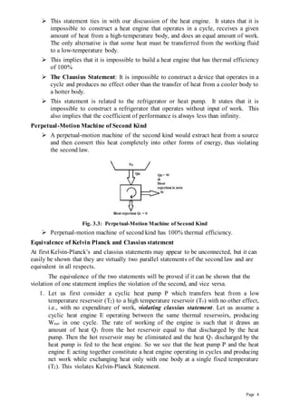
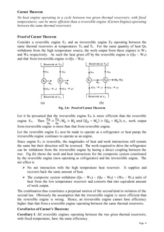
Case 1: Heat is withdrawn at constant temperature
Fig. 3.13: Available and Unavailable Energy: Heat Withdrawn from an Infinite Reservoir
Fig.3.13 represents a reversible engine that operates between a constant temperature
reservoir at temperature T and a sink at temperature T0. Corresponding to heat Q
supplied by the reservoir, the available work Wmax is given by
𝜂 =
𝑊𝑚𝑎𝑥
𝑄
=
𝑇−𝑇0
𝑇
Therefore,
Wmax = Available energy = 𝑄 [
𝑇−𝑇0
𝑇
] = 𝑄 [1 −
𝑇0
𝑇
] = 𝑄 − 𝑇0
𝑄
𝑇
= 𝑄 − 𝑇0 𝑑𝑠
Unavailable energy = 𝑇0 𝑑𝑠
Where 𝑑𝑠 represents the change of entropy of the system during the process of heat
supply 𝑄.
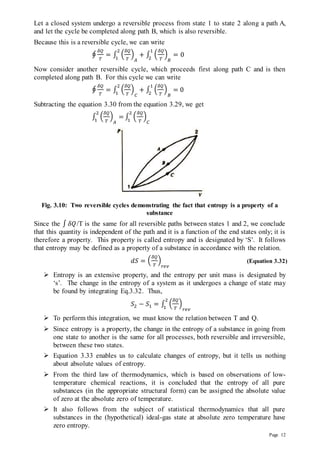
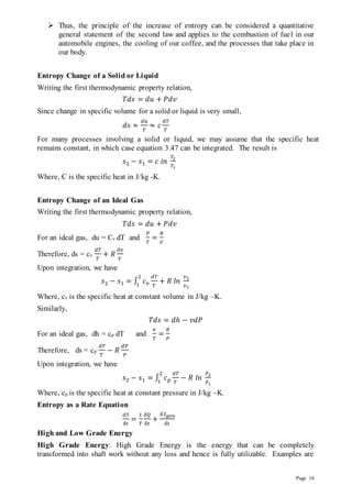
Case 2: Heat is withdrawn at varying temperature.
In case of a finite reservoir, the temperature changes
as heat is withdrawn from it (Fig. 3.14), and as such
the supply of heat to the engine is at varying
temperature. The analysis is then made by breaking
the process into a series of infinitesimal Carnot
cycles each supplying 𝛿𝑄 of heat at the temperature
T (different for each cycle) and rejecting heat at the
constant temperature T0. Maximum amount of work
(available energy) then equals
Fig. 3.14: Available and Unavailable Energy:
Heat Supply at varying Temperature

Wmax = ∫ [1 −
𝑇0
𝑇
] 𝛿𝑄
=∫ 𝛿𝑄 − ∫ 𝑇0
𝛿𝑄
𝑇
=∫ 𝛿𝑄 − 𝑇0 ∫
𝛿𝑄
𝑇
= 𝑄 − 𝑇0 𝑑𝑠
It is to be seen that expressions for both the available and unavailable parts are identical
in the two cases.
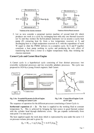
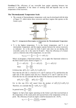
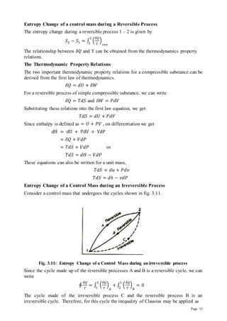
Loss of Available Energy due to Heat Transfer through a Finite Temperature
Difference
Consider a certain quantity of heat Q transferred from a system at constant temperature
T1 to another system at constant temperature T2 (T1>T2) as shown in Fig. 3.15.
Fig. 3.15: Decrease in Available Energy due to Heat Transfer through a Finite Temperature
Difference
Before heat is transferred, the energy Q is available at T1 and the ambient temperature is
T0.
Therefore, Initial available energy, (𝐴𝐸)1 = 𝑄 [1 −
𝑇0
𝑇1
]
After heat transfer, the energy Q is available at T2 and again the ambient temperature is T0.
Therefore, Final available energy, (𝐴𝐸)2 = 𝑄 [1 −
𝑇0
𝑇2
]
Change in available energy = (𝐴𝐸)1 − (𝐴𝐸)2 = 𝑄 [1 −
𝑇0
𝑇1
] − 𝑄 [1 −
𝑇0
𝑇2
]
= 𝑇0 [
−𝑄
𝑇1
+
𝑄
𝑇2
] = 𝑇0
(𝑑𝑆1 + 𝑑𝑆2
) = 𝑇0
(𝑑𝑆)𝑛𝑒𝑡
Where 𝑑𝑆1 = −
𝑄
𝑇1
, 𝑑𝑆2 =
𝑄
𝑇2
and (𝑑𝑆)𝑛𝑒𝑡 is the net change in the entropy of the
combination to the two interacting systems. This net entropy change is called the entropy
change of universe or entropy production.
Since the heat transfer has been through a finite temperature difference, the process is
irreversible, i.e., (dS)net>0 and hence there is loss or decrease of available energy.
The above aspects lead us to conclude that:
 Whenever heat is transferred through a finite temperature difference, there is
always a loss of available energy.
 Greater the temperature difference (T1–T2), the more net increase in entropy and,
therefore, more is the loss of available energy.
 The available energy of a system at a higher temperature is more than at a lower
temperature, and decreases progressively as the temperature falls.

 The concept of available energy provides a useful measure of the quality of
energy. Energy is said to be degraded each time it flows through a finite
temperature difference. The second law may, therefore, be referred to as law of
degradation of energy.
Availability
 The work potential of a system relative to its dead state, which exchanges heat
solely with the environment, is called the availability of the system at that state.
 When a system and its environment are in equilibrium with each other, the system
is said to be in its dead state.
 Specifically, a system in a dead state is in thermal and mechanical equilibrium
with the environment at T0 and P0.
 The numerical values of (T0, P0) recommended for the dead state are those of the
standard atmosphere, namely, 298.15 K and 1.01325 bars (1 atm).
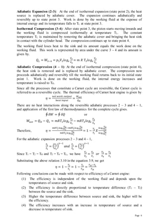
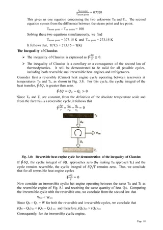
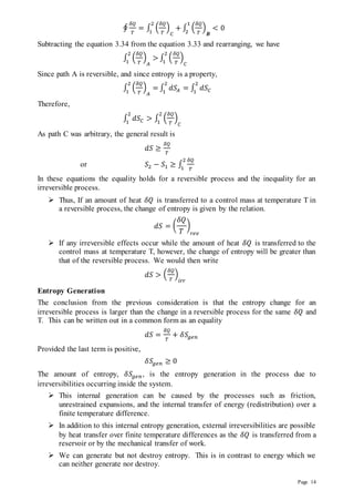
Availability of Non-flow or Closed System
Consider a piston-cylinder arrangement (closed system) in which the fluid at P1, V1, T1,
expands reversibly to the environmental state with parameters P0, V0, T0. The following
energy (work and het) interactions take place:
 The fluid expands and expansion work Wexp is obtained. From the principle of
energy conservation, 𝛿𝑄 = 𝛿𝑊 + 𝑑𝑈, 𝑤𝑒 𝑔𝑒𝑡 ∶ −𝑄 = 𝑊
𝑒𝑥𝑝 + (𝑈0 − 𝑈1
)
The heat interaction is negative as it leaves the system.
Therefore 𝑊
𝑒𝑥𝑝 = (𝑈1 –𝑈0)–𝑄
 The heat Q rejected by the piston-cylinder
assembly may be made to run a reversible heat
engine. The output from the reversible engine
equals
Weng = 𝑄 [1 −
𝑇0
𝑇1
] = 𝑄 − 𝑇0(𝑆1 − 𝑆0 ) (Equ.3.60)
The sum total of expansion work Wexp and the engine
work Weng gives maximum work obtainable from the
arrangement.
Fig. 3.16: Availability of a Non-Flow System
𝑊
𝑚𝑎𝑥 = [(𝑈1–𝑈0)–𝑄] + [𝑄–𝑇0(𝑆1– 𝑆0)]
= (𝑈1–𝑈0)–𝑇0(𝑆1– 𝑆0)
The piston moving outwards has to spend a work in pushing the atmosphere against its
own pressure. This work, which may be called as the surrounding work is simply
dissipated, and as such is not useful. It is given by
𝑊
𝑠𝑢𝑟𝑟 = 𝑃0
(𝑉0 − 𝑉1
)
The energy available for work transfer less the work absorbed in moving the environment
is called the useful work or net work.
Therefore, Maximum available useful work or net work,

(Wuseful)max = Wmax - Wsurr
= (U1 – U0) – T0(S1 – S0) – P0(V0 – V1)
= (U1 + P0V1 – T0S1) – (U0 + P0V0 – T0S0)
= A1 – A0
Where A = (U+P0V – T0S) is known as non-flow availability function. It is a composite
property of the system and surroundings as it consists of three extensive properties of the
system (U, V and S) and two intensive properties of the surroundings (P0 and T0).
When the system undergoes a change from state 1 to state 2 without reaching the dead
state, then
(Wuseful)max = Wnet = (A1 – A0) – (A2 – A0) = A1 – A2
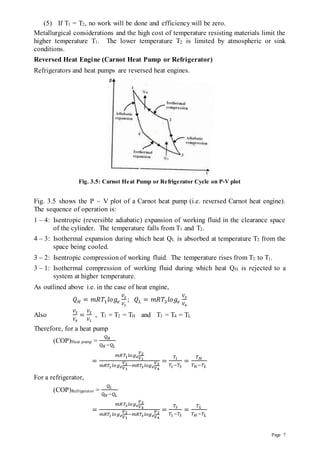
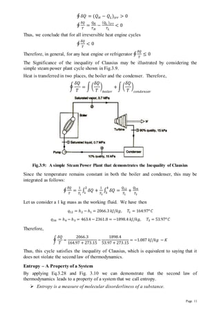
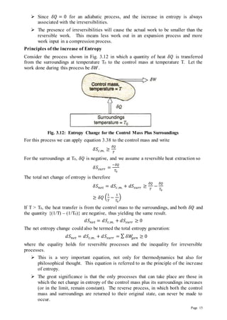
Availability of Steady Flow System
Consider a steady flow system and let it be assumed that the following fluid has the
following properties and characteristics:
Internal energy U, specific volume V, specific enthalpy H, pressure P, velocity C and
location Z.
The properties of the fluid would change when flowing through the system. Let subscript
1 indicate the properties of the system at inlet and subscript 0 be used to designate the
fluid parameters at outlet corresponding to dead state. Further let Q units of heat be
rejected by the system and let the system deliver Wshaft units of work.
𝑈1 + 𝑃1𝑉1 +
𝐶1
2
2
+ 𝑔𝑍1 − 𝑄 = 𝑈0 + 𝑃0𝑉0 +
𝐶0
2
2
+ 𝑔𝑍0 + 𝑊𝑠ℎ𝑎𝑓𝑡
Neglecting potential and kinetic energy changes,
U1 + P1V1 – Q = U0 + P0V0 + Wshaft
H1 – Q + H0 + Wshaft
Therefore, Shaft work Wshaft = (H1 – H0) – Q
The heat Q rejected by the system may be made to
run a reversible heat engine. The output from this
engine equals
Weng = Q [1 −
𝑇0
𝑇1
] = 𝑄 − 𝑇0
(𝑆1 − 𝑆0
) (Equation 3.67)
Therefore, Maximum available useful work or net
work
Wnet = Ws + Weng =(H1 – H0) – Q + Q – T0(S1 – S0)
= (H1 – T0 S1) – (H0 – T0 S0)
= B1 – B0 (Equation 3.68) Fig. 3.17: Availability of a Steady flow System
Where B = (H – T0S) is known as the steady flow availability function. It is composite
property of system and surroundings involving two extensive properties H and S of the
system and one intensive property T0 of the surroundings.
When the system changes from state 1 to some intermediate state 2, the change in steady
flow availability function is given by

dB = (B1 – B0) – (B2 – B0) = B1 – B2
Helmholtzand Gibb’s Functions
For a non-flow process, the maximum work output from the system when T1 = T2 = T0, is
given by
𝑊
𝑚𝑎𝑥 = (𝑈1 – 𝑇1𝑆1) – (𝑈2 – 𝑇2𝑆2) = 𝐴1–𝐴2
 The term (U – TS) is called the Helmholtz function and is defined as the
difference between the internal energy and the product of temperature and entropy.
 The maximum work of the process is equal to the decrease in Helmholtz function
of the system.
In the case of flow process, the maximum work output from the system when T1 = T2 =
T0 and neglecting kinetic and potential energies, is given by
Wmax = (U1 + P1V1 – T1S1) – (U2 + P2V2 – T2S2)
= (H1 – T1S1) – (H2 – T2 S2) = G1 – G2
 The term (H – TS) is called Gibb’s function and is defined as the difference
between enthalpy and product of temperature and entropy.
 The changes of both Helmholtz and Gibb’s functions are called free energy i.e.,
energy that is free to be converted into work. Further, both the Helmholtz and
Gibb’s functions establish a criterion for thermodynamic equilibrium. At
equilibrium, these functions are at their minimum values.
Maxwell Relations
The Maxwell relations can be derived from the different forms of the thermodynamic
property relations discussed earlier such as
𝑑𝑢 = 𝑇𝑑𝑠 − 𝑃𝑑𝑣; 𝑑ℎ = 𝑇𝑑𝑠 + 𝑣𝑑𝑃;
𝐴 = 𝑈 − 𝑇𝑆 (𝑜𝑟) 𝑎 = 𝑢 − 𝑇𝑠 and 𝐺 = 𝐻 − 𝑇𝑆 (𝑜𝑟) 𝑔 = ℎ − 𝑇𝑠
These relations are exact differentials and are of the general form 𝑑𝑧 = 𝑀 𝑑𝑥 + 𝑁 𝑑𝑦.
For exact differentials, we have
(
𝜕𝑀
𝜕𝑦
)
𝑥
= (
𝜕𝑁
𝜕𝑥
)
𝑦
.
Therefore using this relationship we can derive the following equations:
(
𝜕𝑇
𝜕𝑣
)
𝑠
= − (
𝜕𝑃
𝜕𝑠
)
𝑣
; (
𝜕𝑇
𝜕𝑃
)
𝑠
= − (
𝜕𝑣
𝜕𝑠
)
𝑃
(
𝜕𝑃
𝜕𝑇
)
𝑣
= − (
𝜕𝑠
𝜕𝑣
)
𝑇
; (
𝜕𝑣
𝜕𝑇
)
𝑃
= − (
𝜕𝑠
𝜕𝑃
)
𝑇
These four equations are known as the Maxwell Relations for a simple compressible
fluid.
Third Law of Thermodynamics (Nernst Law)
At absolute zero temperature, the entropy of all homogeneous crystalline (condensed) substances
in a state of equilibrium becomes zero. the molecules of a substance in solid phase continually
oscillate, creating an uncertainty about their position. These oscillations, however, fade as the
temperature is decreased, and the molecules supposedly become motionless at absolute zero.
This represents a state of ultimate molecular order (and minimum energy). Therefore, the
entropy of a pure crystalline substance at absolute zero temperature is zero since there is no

uncertainty about the state of the molecules at that instant. This statement is known as the third
law of thermodynamics. The third law of thermodynamics provides an absolute reference point
for the determination of entropy. The entropy determined relative to this point is called absolute
entropy, and it is extremely useful in the thermodynamic analysis of chemical reactions. Notice
that the entropy of a substance that is not pure crystalline (such as a solid solution) is not zero at
absolute zero temperature. This is because more than one molecular configuration exists for such
substances, which introduces some uncertainty about the microscopic state of the substance.

Etd unit iii

Recommended

Recommended

More Related Content

What's hot

What's hot (20)

Similar to Etd unit iii

Similar to Etd unit iii (20)

Recently uploaded

Recently uploaded (20)

Etd unit iii