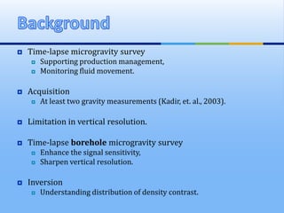
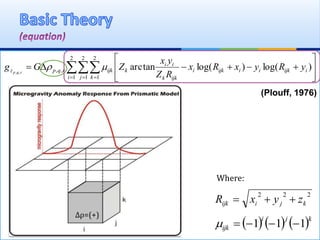
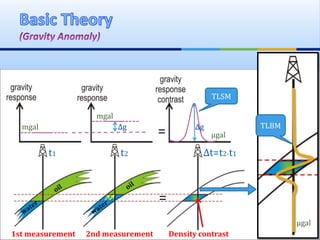
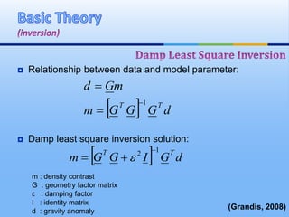
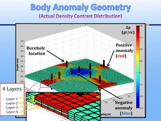
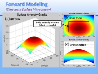
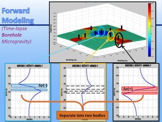
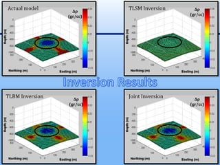
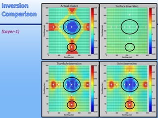
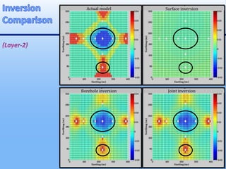
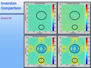
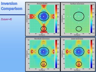
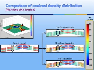
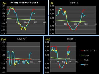
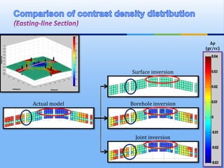
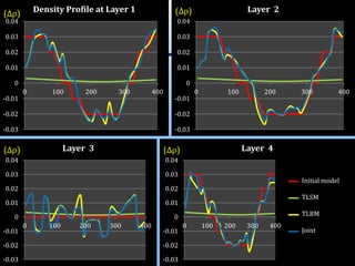
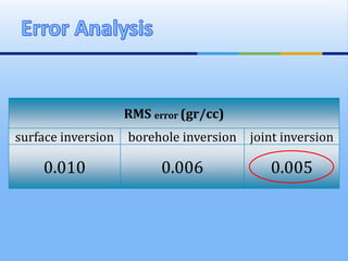
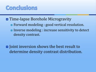
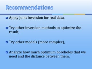
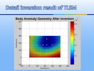
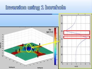
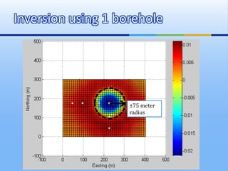
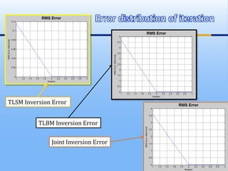
Enhance Gravity Inversion Result Using
Integration of Time-lapse Surface and
Borehole Microgravity
By:
Andika Perbawa(1)(2), Wawan G. A. K(3)
(1)Medco E&P Indonesia
(2) Formerly Geophysical Engineering ITB
(3) Geophysical Engineering ITB
The Bali 2010 International Geosciences Conference and Exposition,
Bali, Indonesia, 19-22 July 2010
 Background
 Basic Theory
 Forward Modeling
 Inverse Modeling
 Analysis
 Conclusions
 Recommendations
 Time-lapse microgravity survey
 Supporting production management,
 Monitoring fluid movement.
 Acquisition
 At least two gravity measurements (Kadir, et. al., 2003).
 Limitation in vertical resolution.
 Time-lapse borehole microgravity survey
 Enhance the signal sensitivity,
 Sharpen vertical resolution.
 Inversion
 Understanding distribution of density contrast.
 Background
 Basic Theory
 Forward Modeling
 Inverse Modeling
 Analysis
 Conclusions
 Recommendations
(Plouff, 1976)
   








2
1
2
1
2
1
,, )log()log(arctan,,
i j
iijkiiijki
ijkk
ii
k
k
ijkrqpz yRyxRx
RZ
yx
ZGg rqp

222
kjiijk zyxR 
     kji
ijk 111 
Where:
∆ρ=(+)
∆gmgal
mgal
1st measurement 2nd measurement
=
=
TLSM
TLBM
Density contrast
t1 t2 ∆t=t2-t1
µgal
µgal
∆g
ρmatrix (gr/cc) ρoil (gr/cc) ρwater (gr/cc) Φ
2.65 0.85 1 27%
ρb= (1-Φ) ρmatrix + Φ (So*ρoil+Sw*ρwater)
1st Condition (100% oil)
ρb(1) = (100% - 27%)2.65 + 27%(100%*0.85 + 0%*1)
ρb(1) = 2.16 gr/cc
2nd Condition (100% water)
ρb(2) = (100% - 27%)2.65 + 27%(0%*0.85 + 100%*1)
ρb(2) = 2.2 gr/cc
∆ρ=ρb(2)-ρb(1)
∆ρ=2.16-2.2
∆ρ=0.04 gr/cc
(Schön, 1995)
ρ1=2
ρ1=2.1
ρ1=2.16
ρ1=2.3
ρ1=2.4
ρ2=2
ρ2=2.1
ρ2=2.2
ρ2=2.3
ρ2=2.4
∆ρ=0
∆ρ=0
∆ρ=0.04
∆ρ=0
∆ρ=0
- =
2nd
condition
1st
condition
Density
contrast
TLBM
response
(+)
(-)
ρ in (gr/cc)
 Relationship between data and model parameter:
 Damp least square inversion solution:
  dGGGm
mGd
TT 1


  dGIGGm
TT 12 
 
(Grandis, 2008)
m : density contrast
G : geometry factor matrix
ε : damping factor
I : identity matrix
d : gravity anomaly
 Background
 Basic Theory
 Forward Modeling
 Inverse Modeling
 Analysis
 Conclusions
 Recommendations
Δρ
(gr/cc)
Borehole
location
Positive
anomaly
(red)
Negative
anomaly
(blue)
4 Layers
Layer-1
Layer-2
Layer-3
Layer-4
(a)3D view (b)map view
(c)Cross section
Body anomaly location
(black rectangle)
Separate into two bodies
∆ρ(-)
∆ρ(+)
 Background
 Basic Theory
 Forward Modeling
 Inverse Modeling
 Analysis
 Conclusions
 Recommendations
Actual Model TLSM Inversion
TLBM Inversion Joint Inversion
Δρ
(gr/cc)
Actual model Δρ
(gr/cc)
TLSM Inversion
Δρ
(gr/cc)
TLBM Inversion Δρ
(gr/cc)
Joint Inversion
Actual model Surface inversion
Borehole inversion Joint inversion
Actual model Surface inversion
Borehole inversion Joint inversion
Actual model Surface inversion
Borehole inversion Joint inversion
Actual model Surface inversion
Borehole inversion Joint inversion
 Background
 Basic Theory
 Forward Modeling
 Inverse Modeling
 Analysis
 Conclusions
 Recommendations
Δρ
(gr/cc)
Actual model
Joint inversion
Borehole inversion
Surface inversion
-0.04
-0.03
-0.02
-0.01
0
0.01
0.02
0.03
0.04
0 100 200 300 400
Density Profile at Layer 1
-0.03
-0.02
-0.01
0
0.01
0.02
0.03
0.04
0 100 200 300 400
Layer 2
-0.03
-0.02
-0.01
0
0.01
0.02
0.03
0.04
0 100 200 300 400
Layer 3
-0.03
-0.02
-0.01
0
0.01
0.02
0.03
0.04
0 100 200 300 400
Layer 4
Layer 4 Origin
Layer 4 from surface
inversion
Layer 4 from All
Borehole inversion
Layer 4 from Join
Inversion
Initial model
TLSM
TLBM
Joint
(∆ρ) (∆ρ)
(∆ρ) (∆ρ)
Δρ
(gr/cc)
Actual model
Joint inversion
Borehole inversion
Surface inversion
-0.03
-0.02
-0.01
0
0.01
0.02
0.03
0.04
0 100 200 300 400
Density Profile at Layer 1
-0.03
-0.02
-0.01
0
0.01
0.02
0.03
0.04
0 100 200 300 400
Layer 2
-0.03
-0.02
-0.01
0
0.01
0.02
0.03
0.04
0 100 200 300 400
Layer 3
-0.03
-0.02
-0.01
0
0.01
0.02
0.03
0.04
0 100 200 300 400
Layer 4
Layer 4 Origin
layer 4 from surface
inversion
Layer 4 from all
borehole inversion
Layer 4 from join
inversion
Initial model
TLSM
TLBM
Joint
(∆ρ) (∆ρ)
(∆ρ) (∆ρ)
RMS error (gr/cc)
surface inversion borehole inversion joint inversion
0.010 0.006 0.005
 Background
 Basic Theory
 Forward Modeling
 Inverse Modeling
 Analysis
 Conclusions
 Recommendations
 Time-lapse Borehole Microgravity
 Forward modeling : good vertical resolution.
 Inverse modeling : increase sensitivity to detect
density contrast.
 Joint inversion shows the best result to
determine density contrast distribution.
 Background
 Basic Theory
 Forward Modeling
 Inverse Modeling
 Analysis
 Conclusions
 Recommendations
 Apply joint inversion for real data.
 Try other inversion methods to optimize the
result,
 Try other models (more complex),
 Analyze how much optimum boreholes that we
need and the distance between them,
Thank You
Back Slide
Detail inversion result of TLSM
Inversion using 1 borehole
Δρ
(gr/cc)
Inversion using 1 borehole
±75 meter
radius
Error distribution of iteration
TLSM Inversion Error
TLBM Inversion Error
Joint Inversion Error
 Resolution : 1-20 µgal
 Gas-oil  ± 2 µgal
 Gas-water  ± 5 µgal
 Oil-water  0.7-3 µgal
 Accessable casing up to 5½ inch.
 14 degree from vertical.
(Nabighian, et. al., 2005)
Instrument
Instrument of
boreholegravitymeter.
(Goodell, R. R., 1964).

Enhance Gravity Inversion Result Using Integration of Time-lapse Surface and Borehole Microgravity

Editor's Notes

  • #2 bAss.wr.wb. Good morning ladies and gantleman.. Glad to see u here.. And thanks for coming to attend in my dry run presentation with title “Enhance Gravity Inversion Result Using Integration of Time-lapse Surface and Borehole Microgravity”.
  • #3 This is outline that i propose Start from .... And recommendations
  • #5 This is outline that i propose Start from .... And recommendations
  • #6 Gravity attraction in vertical direction caused of prismatic body in subsurface shown as equation fom plouff, 1976......
  • #9 This is the schematic TLBM anomaly. Actualy, what is time-lapse microgravity anomaly? TLM is like this... There are 2 measurement in certain time interval... And we measure the differences gravity anomaly from a both of measurement. This is the final condition (2nd measurement) This is the initial condition (1st measurement) Then this is the density differences (density contrast) The density contrast thats we call body gravity anomaly... Then this is the TLBM response in borehole.
  • #10 To understand about contrast density distribution in our body, we hate to invert gravity anomaly by using inversion step. In this paper i use damp least square inversion method.
  • #11 This is outline that i propose Start from .... And recommendations
  • #12 This is a model that i create... This model looks like anticline with 4 way dip structure. From 4 ways there are injection activity represented by red colour (positive anomaly) While in the crest of anticline there is production activities that represented by blue colour (negative anomaly) Injection produce positive anomaly because it increasing density of pore fluid reservoir. From original oil replaced by water which is higher density. Production produce negative anomaly because it decreasing density of pore fluid reservoir. From more oil to less oil which is makes density decrease.
  • #13 This is the forward modeling of TLSM. Usually, The gravity anomaly distribusion of TLSM is quite similar with distribusion of contrast density. But, in this model is different. Why? It could be caused by small geometry of body. My body is around 0.12 KM square. Is too small for being the field. Then this is the challenge for geophysicist if we get the problem like this. The important thing in this picture is i cannot measure the accuracy in vertical direction. We just know the distribution in lateral direction. So, to handle this problem TLBM can answer that.
  • #15 This is outline that i propose Start from .... And recommendations
  • #21 This is outline that i propose Start from .... And recommendations
  • #22 This is northing line section of contrast density distribution. Joint inversion gives the best result among them
  • #23 Joint inversion have the best fit to initial model than another inversion method
  • #24 This is easting-line section of contrast density distribution. Joint inversion gives the best result among them
  • #25 Joint inversion have the best fit to initial model than another inversion method
  • #26 This is RMS error of density distribution over three inversion method. And joint inversion has the lowest error than TLSM or TLBM.
  • #27 This is outline that i propose Start from .... And recommendations
  • #29 This is outline that i propose Start from .... And recommendations
  • #32 Last sentences i would like to share is. When the man brains is thinking about oil and gas exploration, it simple and cheap if we optimize our production field first, Monitoring is a way to make sure is our injection works well or not... Then, time-lapse microgravity born to answer that. Again, thank you for coming here... And its time for discussion and answer-question time.