Download to read offline


![12 mentor.com/mechanical
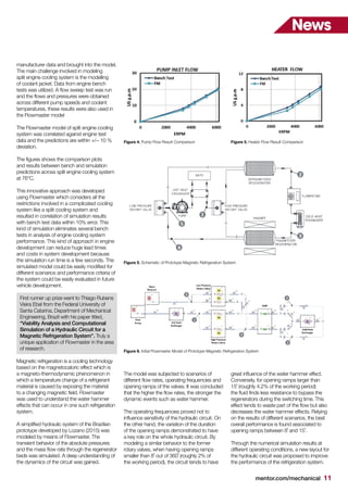
Based on the obtained results in this work,
the most suitable solution is to include a
proportional returning valve before the high
pressure valves and after the low pressure
valves. Such a device would be capable of
absorbing the water hammer effects and to
make the flow through the regenerators’ beds
smoother. Even though the system would
require higher pumping capacity, due to flow
bypass, an estimation of the novel hydraulic
circuit would have a COP of 1.34 and a
second law efficiency of η2nd = 9.55% (the
actual system had a maximum second law
efficiency of η2nd = 1.16%).
Second Runner up Award went to “Study
on the one-dimensional carriage and
ventilation system of high-speed train”
from Yifei Zhu, Yugong Xu, Xiangdong Chen
of the School of Mechanical Electronic
and Control Engineering, Beijing Jiaotong
University, Beijing, China.
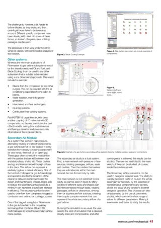
Their work investigated the interaction of the
outside environment and the interior airflow
through the ventilation system of a high
speed train during operation. In past studies,
this interaction has been ignored resulting
in significant inaccuracies in the results.
The composition of the complex ventilation
system includes: air inlet, grill, controllable
dampers, ducts, air conditioning units, air
orifice, return air valves, and waste discharge
units. Due to the overall complexity and length
vs. the hydraulic diameter of the ducts, a
1D simulation with Flowmaster was the only
practical solution to the simulation problem.
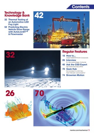
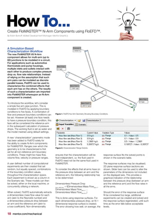
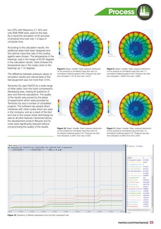
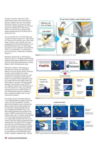
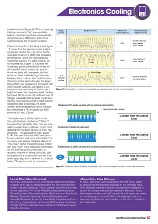
Figure 9 is the 3D CAD drawing of the
ventilation of the high-speed train carriage. It
consists of a combination of fresh air ventilation
system parts, exhaust section and return air
section together.
Because the model is so complicated, a
simplification process was used to reduce the
complexity of the model. This included:
1. The pressure protection valve is open in
normal operation, so it was ignored,
2. Air conditioning mixing box. This is just
a confluence of container shaped like a
Y-pipe, the drag coefficient is small, and
therefore considered as a modeling point
of convergence, and
3. Because the study was only interested
in the airflow distribution and not
temperature the components of the
air conditioning and heating units were
simplified to resistance elements based
on local resistance.
The supply duct system lines consists mainly
of long straight pipes with only a few individual
bends and corners which have very small
additional resistance relative to the long pipes
so they were omitted as well.
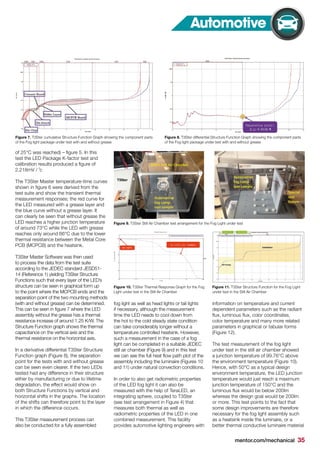
After these simplifications were made, the
Flowmaster model was constructed as shown
in figure 10.
Results of the simulation showed that the new
outlet flow, exhaust port flow, return airflow,
and airflow rate of each branch meet design
conditions and the calculation results are
consistent with the actual operating point of
the ventilation system, which demonstrates
the rationality and accuracy of the simulation
model. This modeling approach will be used to
predict other environmental conditions inside
the train carriage.
From these award winning papers it is easy
to see the versatility of Flowmaster and how
creative engineers from around the world are
finding new and innovative ways to use it to
solve their simulation and design problems.
References:
[1] C, S., Sundaram, V., and S, S., "Simulation
of Split Engine Cooling System," SAE
Technical Paper 2015-26-0196, 2015,
doi:10.4271/2015-26-0196
[2] Thiago Rubens Vieira Ebel, "VIABILITY
ANALYSIS AND COMPUTATIONAL
SIMULATION OF A HYDRAULIC CIRCUIT
FOR A MAGNETIC REFRIGERATION
SYSTEM"Florianópolis - SC, February, 2016
[3] Yifei Zhu, Yugong Xu, Xiangdong Chen,
" Study on the one-dimensional carriage
and ventilation system of high-speed train"
International Power, Electronics and Materials
Engineering Conference (IPEMEC 2015)
Figure 8. Flowmaster Model of Redesigned Prototype Magnetic Refrigeration System
Figure 7. Typical Water Hammer results in the System
Figure 9. 3D CAD Drawing of Ventilation System of High-
Speed Train Carriage
Table 1. Comparison of Flowmaster Simulation Results Vs Actual Operating Point Values
Figure 10. Flowmaster Network of Ventilation System of
High-Speed Train Carriage](https://image.slidesharecdn.com/afb16ffc-081e-48c5-993e-067049b05c6c-161109101320/85/engineering-edge-vol-5-iss-2-LR-12-320.jpg)


![36 mentor.com/mechanical
to reduce the LED junction temperature
and increase the luminous flux, while
at the same time increasing the lifetime
expectancy of the fog light.
Summary
This MicReD T3Ster/TeraLED thermal
characterization testing process can
be conducted at various stages of an
automotive fog light’s development from the
initial LED selection process from different
vendors, to its lifetime tests, up to the
point where the LEDs are mounted on the
PCB, or even in a full fog light assembly
to validate the quality of the assembly.
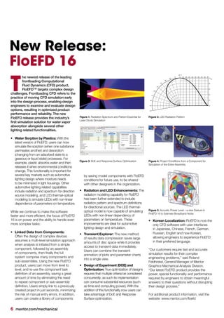
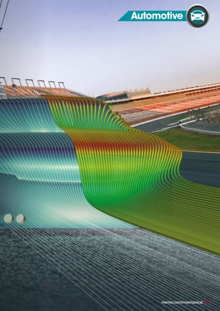
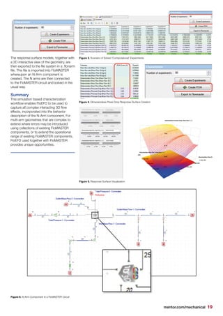
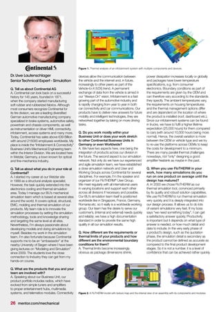
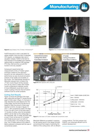
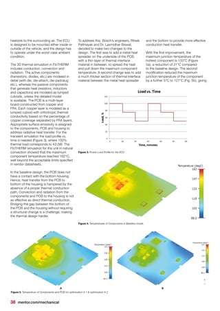
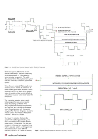
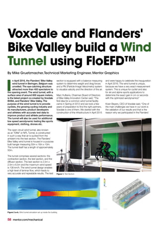
A combination of thermal transient
measurement data from T3Ster coupled to
thermal simulation with a CAD-embedded
3D CFD code like FloEFD (Figure 13) can
then be used to provide highly accurate
simulations this predicting LED assembly
thermal performance, and ultimately helping
to ensure fog light reliability over its lifetime.
Reference
[1] JEDEC, "JESD51-14 Transient Dual
Interface Test Method for the Measurement
of the Thermal Resistance Junction to Case
of Semiconductor Devices with Heat Flow
Through a Single Path," vol. JESD51-14, ed.
http://www.jedec.org/standards-documents/
results/51-14: Joint Electron Device
Engineering Council, November 2012, p. 4
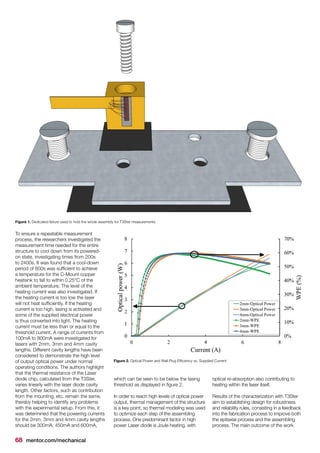
Figure 12. TeraLED output variables for the Fog Light under test
Figure 13. Automotive Lighting Workflow for Measurement and Simulation of LED Components](https://image.slidesharecdn.com/afb16ffc-081e-48c5-993e-067049b05c6c-161109101320/85/engineering-edge-vol-5-iss-2-LR-36-320.jpg)


![52 mentor.com/mechanical
ould the era of the electric
car finally be upon us? The
answer is yes, but there is
still a long way to go. A major
concern for consumers of electric vehicles
has been that the range of these vehicles
has shown to be extremely variable with
ambient temperature, [1,2] The ability
to understand the effects that potential
factors will have to the range of any EV
is critical to creating a better design and
thus improving the product for customers,
ultimately driving increasing adoption.
For this reason, the earlier an engineer is
able to quantify how different factors will
affect the EV, the better, and one of the
most efficient ways to do this is through
computer simulation.
The purpose of this study was to quantify
the ability to capture at least some of these
effects using a co-simulation approach to
represent different segments of the vehicle.
The results were then compared against
published empirical data collected by
Charged[3] magazine to determine how well
the approach fits real world test results. The
co-simulation was done using three different
software packages to model different parts of
the vehicle.
C
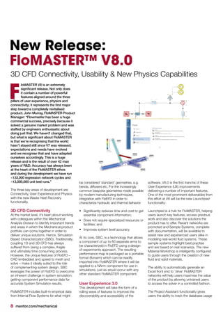
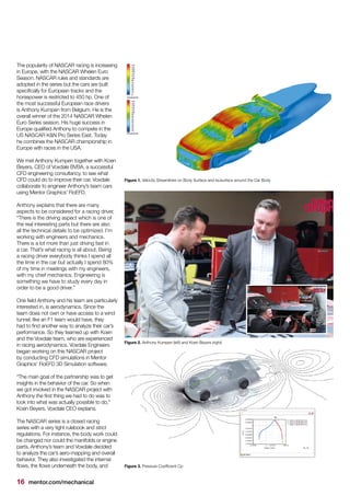
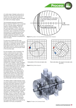
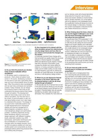
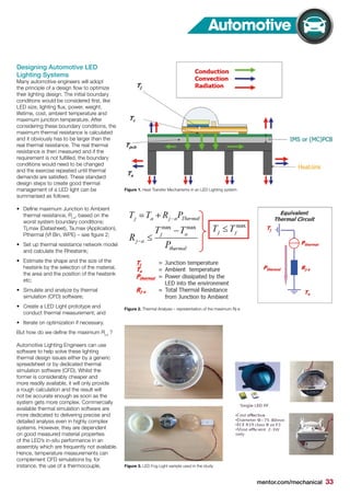
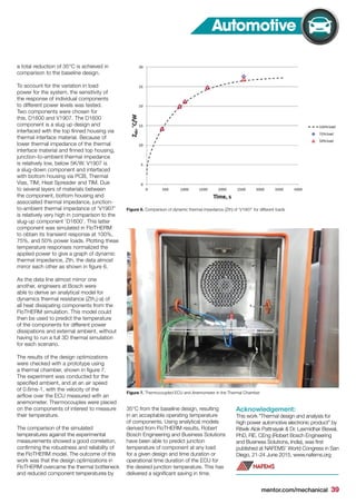
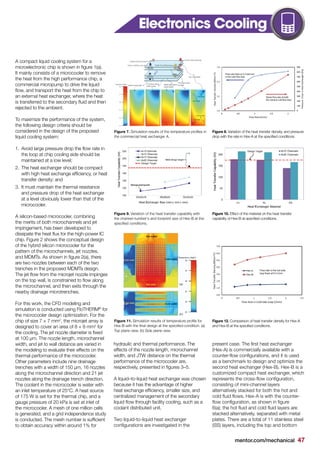
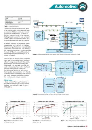
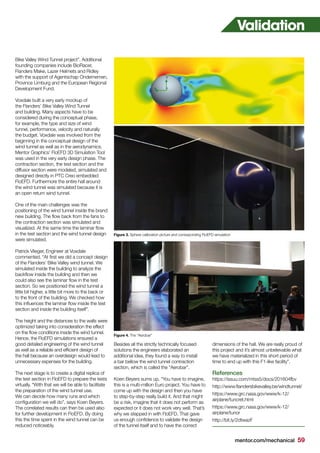
Figure 1. C/3 Discharge Curve for a Single 70/30 LMO/NMC 33Ah Cell
Table 1. Battery Design Parameters
Predicting EV
Drive Range
Battery Pack Model
The performance of the battery was modeled
using EC Power’s AutoLion-STTM
. The pack
and cells were loosely configured to represent
the first generation Nissan Leaf design. The
model was responsible for handling three
aspects of the simulation, calculating the
temperature of the battery pack, calculating
the pack voltage, and calculating the State
of Charge (SoC).
From the vehicle model, the battery
model received a total pack power
requirement with the simulation continuing
until the battery model reached a SoC
state of 20%.
Parameter Value
Energy 24 kWh
Cells in Series 96
Cells in Parallel 2
Cell Shape Prismatic
Cathode 70/30 LMO/NMC
Anode Graphite
By Doug Kolak,Technical Marketing
Engineer, Mentor Graphics](https://image.slidesharecdn.com/afb16ffc-081e-48c5-993e-067049b05c6c-161109101320/85/engineering-edge-vol-5-iss-2-LR-52-320.jpg)
![mentor.com/mechanical 53
Vehicle Model
The vehicle portion of the model was
constructed in MATLAB Simulink®
. The
vehicle model acted as the platform for the
entire co-simulation collecting and distributing
data between models. As part of this task,
the model also set several of the initial
conditions including: ambient, cabin, and
battery temperatures; cabin set-point; drive
cycle and driver aggressiveness factor.
The vehicle model was also responsible for
determining the total power requirement
of the vehicle. This included the effects of
drag, braking, drivetrain inefficiencies, and
propulsion/regeneration from the electric
motor. The model also separately determined
the cooling fan on/off state with the required
power added to the total requirement if
necessary.
Cabin Thermal & Battery
Cooling Model
The cabin and battery cooling air portions
of the model were constructed in Mentor
Graphics 1D Computational Fluid Dynamics
tool, Flowmaster. The primary purpose of
the Flowmaster model was to calculate the
power required to maintain the given set-
point temperature of the cabin at the different
ambient temperatures and vehicle velocities.
To accomplish this, the Automotive 1D Cabin
component was used to calculate the average
cabin temperature as a function of inlet airflow
rate, air temperature, and vehicle velocity. The
model was able to account for the difference
in external heat transfer based on when the
vehicle was moving or stationary as well as the
heat input due to solar radiation.
The HVAC system was modeled as a
simplified heating or cooling generation
component. This component added or
removed heat to the airflow entering the cabin
based on the feedback from Flowmaster‘s
PID controller. A Coefficient of Performance
(CoP) of two was used to account for the
inefficiencies in the HVAC system.
The Flowmaster model was also responsible
for calculating the temperature of the battery
pack cooling air and the cooling fan power
requirement. If the temperature rose high
enough, the vehicle model would signal
that the fan should be running. Under these
circumstances, Flowmaster would calculate
the heat added to the airflow due to the
fan inefficencies as well as the power the
fan required. The overall Flowmaster power
requirement fed back to the vehicle level
model to be included in the total power
requirement of the battery.
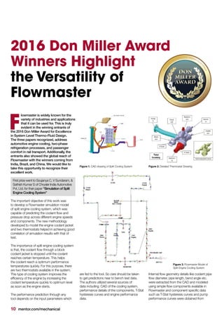
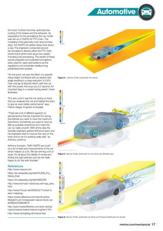
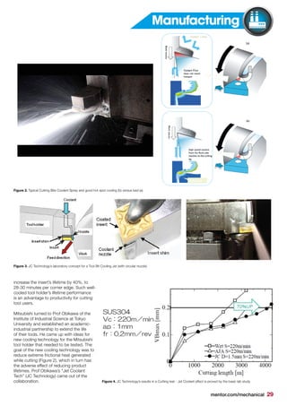
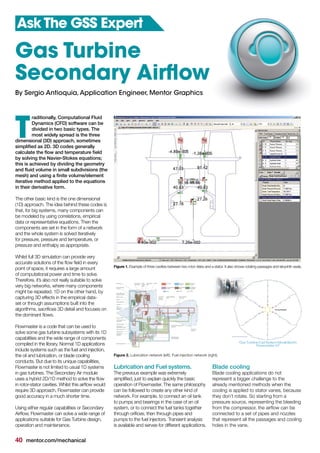
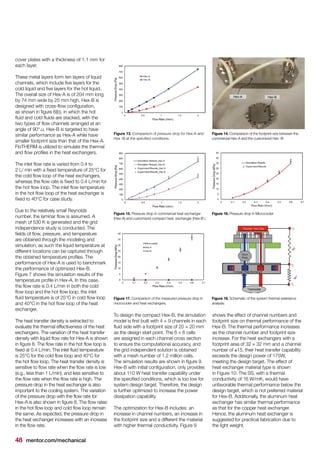
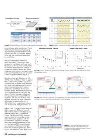
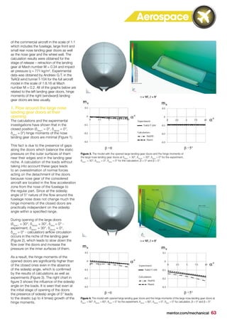
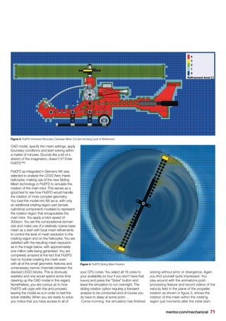
Figure 2. Predicted Drive Range for different Ambient Pressures vs. Published Data
Results and Conclusions
The purpose of the study was to understand
how different factors effected the overall drive
range of the vehicle through simulation. The
three factors chosen for the study were driver
aggressiveness, cabin set point temperature,
and ambient temperature. Several values for
each factor were used in the study as a full
factorial study:
Each co-simulation ran for between five
and ten minutes ending once the SoC of
the battery model reached 20%. In total,
the seventy-two studies were run over two
days requiring approximately eight hours of
engineering time.
The results can also be shown against the
data publish in Charged magazine. In figure 2,
the yellow band represents the middle 50% of
test data collected while the solid purple line
represents the longest 10% of drive ranges.
Overall the trends seen from the analysis, are
what was expected before the study began.
As shown in figure 2, the results were on the
upper end of what was seen by Charged
magazine as part of their data collection.
Further refinement to the estimates for
drive cycle and driver aggressiveness could
improve this correlation. The model could also
be further developed, including more accurate
data for the cabin materials as well as the
performance of the HVAC system.
With improvements to the model the spread
of distance results would likely decrease to
be more consistent with test data. The study
showed that while drive range information
can be determined through test, using
a co-simulation approach, a reasonable
approximation was possible from a full
factorial of driving scenarios in less than one
engineering day.
Literature
[1] Heather Hunter, AAA News Room,
“Extreme Temperatures Affect Electric Vehicle
Driving Range, AAA Says,” March 20, 2014
http://newsroom.aaa.com/2014/03/extreme-
temperatures-affect-electric-vehicle-driving-
range-aaa-says/
[2] Consumer Reports News, “Winter chills
limit range of the Tesla Model S electric
car,” February 15, 2013. http://www.
consumerreports.org/cro/news/2013/02/w
inter-chills-limit-range-of-the-tesla-model-s-
electric-car/index.htm
[3] “FleetCarma Goes Deep into the Data”,
Charged. Pg. 56-61. Jan/Feb 2015.
[4] Kolak, D., Shaffer, C., Marovic, B., Sinha, P.
Prediction of EV Drive Range Reduction
under Extreme Environmental conditions
using Computer Aided Engineering Tools
June 2016, EEHE2016
Automotive
Table 2. Study Factors and Values
Factor Values
Driver Aggressiveness 0.8, 1.0, 1.2
Cabin Set Point Temperature 15, 20, 24 (°C)
Ambient Temperature -10, 0, 10, 20, 30, 40, 50 (°C)](https://image.slidesharecdn.com/afb16ffc-081e-48c5-993e-067049b05c6c-161109101320/85/engineering-edge-vol-5-iss-2-LR-53-320.jpg)


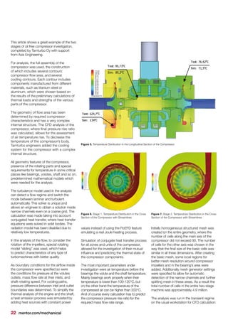
![o investigate the impact of
the fluid flow on the aircraft’s
units CFD (Computational Fluid
Dynamics) methods based
on the numerical calculation of the
hydrodynamic equations becomes
widely used along with the conventional
analytical approaches and experimental
tests. Continuously developed and
improved CFD methods can serve
as a good alternative of the natural
experiments in solving many practical
problems [1].
Thus, at the design stage of the landing
gear doors production often without being
able to carry out the natural experiment,
designers need to have level
of aerodynamic loads
acting on the
closed doors at high speed of aircraft as
well as during aircraft’s maneuvers with the
opened doors and gear release/retraction.
The aerodynamic loads data obtained
from CFD analysis gives the possibility to
estimate the doors strength and define
characteristics of the opening actuator, run
the optimization of the kinematic connection
between small rear doors with the landing
gear strut. For instance, for the considered
aircraft the initial variant of the small landing
gear door rod mounting to the
landing gear main fitting has
been replaced
T
Cleared
for Landing
Numerical Methods for the Definition of the
Hinge Moments of the Nose Landing Gear
Doors of the Commercial Aircraft
By O.V. Pavlenko,TsAGI,A.V. Makhankov,A.V. Chuban, Irkut Corporation
60 mentor.com/mechanical](https://image.slidesharecdn.com/afb16ffc-081e-48c5-993e-067049b05c6c-161109101320/85/engineering-edge-vol-5-iss-2-LR-60-320.jpg)

![62 mentor.com/mechanical
by the mounting to the landing gear strut to
reduce the loads on the rod. The calculation
results obtained for the selected variant of
the doors were confirmed experimentally
that indicates good accuracy of the modern
software.
The results of the numerical study of
aerodynamic loads on the nose landing
gear doors demonstrated in this paper were
obtained in ANSYS®
Fluent and Mentor
Graphics FloEFD™ software, based on
the solution of the Reynolds averaged and
Favre averaged Navier-Stokes equations
accordingly.
The calculation in ANSYS Fluent software
(license number 501024) was done using
the structured computational mesh (about
6 million cells) with « κ - ε realizable»
turbulence model (κ - ε method based on
a simultaneous solution of the momentum
transport equations, the kinetic energy
and the dissipation rate equations) with
the enhanced modeling of turbulence
parameters near the wall and with taking
into account the influence of the pressure
gradient. The solved equations were
approximated with a finite-volume scheme
of the second order.
The numerical study in FloEFD software was
performed using rectangular computational
mesh adapted to the surface (about
2.5 million cells) [3]. To speed up the
calculations the local meshes with the
increased mesh resolution around the nose
of the fuselage and landing gear doors
FloEFD Fluent
Figure 2. Streamlines on the doors and in the niche at δdoor1
= 30°, δdoor2
= 0°.
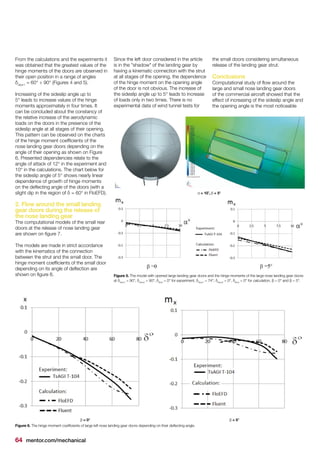
Figure 1. The model with the closed landing gear doors and hinge moments of the large left nose landing gear doors at
δdoor1
= 0°, δdoor2
= 0°, δstrut
= 0°, β = 0° and β = 5°.
α = 10˚, β = 5°
were used. The automatically adapting
computational mesh with concentration in
the areas of high gradients of velocity was
applied. It should be noted that FloEFD
uses a relatively small number of cells of
the computational mesh as far as in case of
a low resolution of the boundary layer the
theory based on the Prandtl boundary layer
hypothesis is applied. Turbulence model
used in FloEFD bases on the modified
model with damping functions proposed by
Lam and Bremhorstom [4].
The calculations of the hinge moments of
the nose landing gear doors were performed
for the three-dimensional model of the part](https://image.slidesharecdn.com/afb16ffc-081e-48c5-993e-067049b05c6c-161109101320/85/engineering-edge-vol-5-iss-2-LR-62-320.jpg)
![mentor.com/mechanical 65
for the large doors with a big aerodynamic
surface.
Loads acting on the small doors
kinematically connected with the landing
gear strut depend on the sideslip angle
much less. The dependence of the loads
on the small doors on their opening angle
occurs only in the presence of sideslip
angle.
The results of calculations performed in
Fluent and FloEFD presented in this article
show good agreement with the experimental
data and demonstrate the ability to use
these software for the calculation of the
loads on the landing gear doors during the
design stages.
Figure 7. The computational models with different angles of the strut, large and small doors.
δstrut
= 15°, δlarge door
= 74°,
δsmall door
= 14.304°
δstrut
= 60°, δlarge door
= 74°,
δsmall door
= 55.378°
δstrut
= 30°, δlarge door
= 74°,
δsmall door
= 27.846°
δstrut
= 75°, δlarge door
= 74°,
δsmall door
= 68.125°
δstrut
= 45°, δlarge door
= 74°,
δsmall door
= 41.498°
δstrut
= 100°, δlarge door
= 74°,
δsmall door
= 72.232°
Figure 8. The hinge moment coefficients of small left nose landing gear doors depending on their deflecting angle.
β = 0° β = 5°
The use of FloEFD software does not
require thorough preparation of the
computational model as far as this tool uses
an automatic meshing and it is embedded in
all modern CAD-software. On the contrary
the use of Fluent software with structured
mesh requires long preparation of the
computational model but allows to perform
a fast calculation.
References
[1] Platonov D.V., Minakov A.V., Dekterev A.A.,
Kharlamov E.B., Comparative Analysis of CFD-
packages SigmaFlow and Ansys Fluent on the
solution of the laminar problems // Bulletin of
the Tomsk State University, 2013, №1 (21)
[2] Pavlenko O.V., Determination of loads on
the nose landing gear doors and strut of a
commercial aircraft based on the numerical
solution of the Navier-Stokes equations //
TVF. 2011, Volume LXXXV, №2 (703), p.
19-25
[3] Dr. A. Sobachkin, Dr. G. Dumnov
Numerical Basis of CAD-embedded CFD,
NAFEMS World Congress 2013
[4] Lam, C.K.G. and Bremhorst, K.A. (1981)
Modified Form of Model for Predicting
Wall Turbulence, ASME Journal of Fluids
Engineering, Vol.103, pp. 456-46
Aerospace](https://image.slidesharecdn.com/afb16ffc-081e-48c5-993e-067049b05c6c-161109101320/85/engineering-edge-vol-5-iss-2-LR-65-320.jpg)
![By Roberto Mostallino, M. Garcia1
,Y. Deshayes2
,A. Larrue1
,Y. Robert1
,
E.Vinet1
, L. Bechou2
, M. Lecomte1
, O. Parillaud1
, and M. Krakowski1
1 III-V lab, France 2 Laboratoire IMS, Université de Bordeaux, France.
he demand of high power
Laser diodes is ever increasing.
Especially devices in the 910-
980nm range are used for fibre
laser pumping, material processing,
solid-state laser pumping, defense and
medical/dental applications.
Critical to the device’s operation is its ability
to convert the input electrical power into
output optical power with high efficiency,
since such devices need a stable wavelength
that is affected by the device temperature.
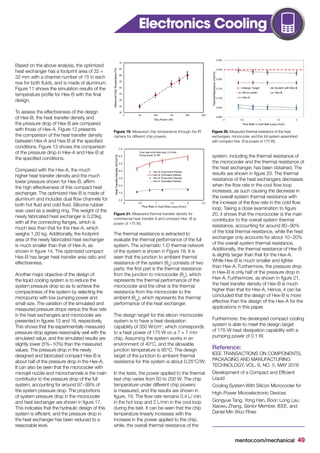
Researchers at III-V Lab/THALES Research
Technology in Palaiseau, France have
recently developed a structure for a diode
laser based on a Al-free Large Optical
Cavity (LOC), [1], and a uniform distributed
feedback grating (DFB) and processing
techniques that are able to achieve the best
up-to-date optical performances with an
optimized thermal management through one
of the lower thermal resistance. In such a
context, low thermal resistance of the
entire assembly (< 2K/W) is
difficult to measure
through classical optical techniques. Detail
and precise characterizations of the high
power Laser diode assembly have been
carried out at IMS Laboratory (CNRS UMR
5218) from the University of Bordeaux.
Regular practice is to use an infrared camera,
spectral measurements vs temperature
and the pulse electrical method. Infrared
cameras are not particularly accurate or
required emissivity calibration and spectral
measurements that monitor temperature
variations versus drifts of the central
wavelength, are not well-suited for these
high power laser diodes mainly due to their
spectral multimode behavior. Therefore,
the two research teams devised a new
measurement approach based on Mentor
Graphics’ T3Ster®
equipment. The method
is well-known for conventional electronic
devices and LEDs, being a crucial technique
for understanding both the
thermal management of
the structure and its improvement through
design for reliability. Part of this approach
involved mixing 2D finite element modeling
of the Laser diode and structure functions
created using the T3Ster-Master software
in order to correctly predict the temperature
distribution within the structure.
Many papers have been recently published
on the use of T3Ster, especially in the field of
thermal resistance extraction of high-power
GaN-based LEDs, as reported in references
2 to 4. However, application to laser diodes,
particularly for a high-power diode laser
emitting at 975nm, has been published
publicly very recently (See reference in
acknowledgements).
T
Achieving a 60%
Efficient Laser Diode
Design With Optimized
Thermal Management
66 mentor.com/mechanical](https://image.slidesharecdn.com/afb16ffc-081e-48c5-993e-067049b05c6c-161109101320/85/engineering-edge-vol-5-iss-2-LR-66-320.jpg)

![mentor.com/mechanical 69
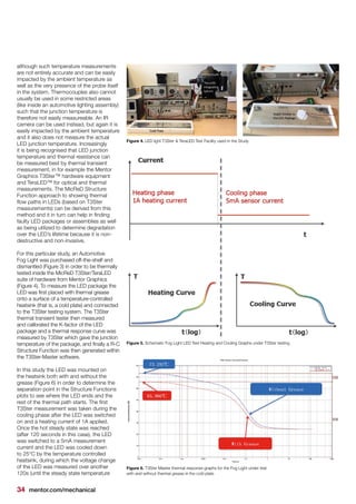
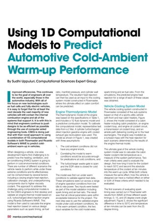
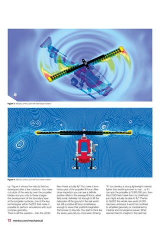
Figure 4. Cumulative Structure Function of three-cavity length laser. The numbers on the plot correspond to the
different parts in figure 1.
Figure 3. Optical spectrum of a DFB 4mm cavity laser at 60°C in CW operation at 5A.
emphasizes a laser diode that has a wall
plug efficiency above 60%, that remains
stable when driven with a current of up to
8A, exhibits a side mode suppression ratio
greater than 30dB (so that emits strongly at
975nm and much more weakly either side
of that peak frequency). The spectral line
width at 975nm is less than 1nm, putting this
device among the very few laser diode with
stabilization wavelength thanks to internal
gratings (DFB). This laser diode shows also
one of the best thermal resistance reported in
literature [5].
The Structure Function is shown in figure 4,
in which each part of the structure can be
identified by the numbers corresponding
to those in figure 1. From the Structure
Functions it is possible to extrapolate the
thermal resistance of the 2, 3 and 4mm
cavity length laser diode chips to be 3.2,
2.8 and 1.5°C /W respectively, dealing with
a more reliable approach than using the
classical optical method. Such technique
allows to investigate the contribution of each
part of the laser diode assembly. Moreover,
T3Ster provides the opportunity to identify
any atypical behavior for the device, such as
assembly interface degradation.
Acknowledgements:
This article is abstracted from the paper
“THERMAL INVESTIGATION ON HIGH
POWER DFB BROAD AREA LASERS AT
975nm, WITH 60% EFFICIENCY” by R.
Mostallino1,2
, M. Garcia1
, Y. Deshayes2
, A.
Larrue1
, Y. Robert1
, E. Vinet1, L. Bechou2
, M.
Lecomte1
, O. Parillaud1
, and M. Krakowski1
1 III-V lab, 1 avenue Augustin Fresnel 91767
Palaiseau, France
2 Laboratoire IMS, Université de Bordeaux,
CNRS UMR 5218, 351 Cours de la
Libération, 33405 Talence Cedex, France.
References:
[1] N. Michel, M. Calligaro, M. Lecompte,
O. Parillaud, and M. Krakowki, “High wall-
plug efficiency diode lasers with an Al free
active region at 975nm,” in Photonics West
Conference, San Jose, USA, 2009, vol.
Paper 7198–53.
[2] S. Shanmugan and D. Mutharasu,
“Thermal transient analysis of high power
led employing spin coated silver doped zno
thin film on al substrates as heat sink,” J.
Optoelectron. Biomed. Mater., vol. 7, no. 1,
pp. 1–9, 2015.
[3] S. Shanmugan and Mutharasu, D.,
“Thermal transient analysis of high power
LED tested on Al2O3 thin film coated Al
substrate,” Int. J. Eng. Trends Technol., vol.
30, no. 6, p. 6, 2015.
[4] C. Jong Hwa and S. Moo Whan, “Thermal
investigation of LED lighting module,”
Microelectron. Reliab., vol. 52, no. 5, pp.
830–835, 2012.
[5] A. Pietrzak, R. Hülsewede, M. Zorn,
O. Hirsekorn, J. Sebastian, J. Meusel, P.
Hennig, P. Crump, H. Wenzel, S. Knigge,
A. Maaßdorf, F. Bugge, and G. Erbert,
“Progress in efficiency-optimized highpower
diode lasers,” in SPIE, 2013, vol. 8898, pp.
08–22.
Electronics Cooling](https://image.slidesharecdn.com/afb16ffc-081e-48c5-993e-067049b05c6c-161109101320/85/engineering-edge-vol-5-iss-2-LR-69-320.jpg)


The document is a newsletter from Mentor Graphics announcing new releases and features of their computational fluid dynamics (CFD) and thermal analysis software products. Some key points: - FloEFD 16 includes new capabilities for simulating water vapor absorption in plastics and improved radiation modeling for automotive lighting design. - A new version of FloMASTER (V8.0) features improved 3D CFD connectivity through Simulation Based Characterization, which allows 1D system models to be coupled with 3D CFD component models. - Usability improvements include a new user interface and physics additions like a waste heat recovery capability. - Awards were given for applications of the software in automotive, aerospace


