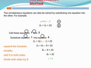
electric calculation for power engineering

Electrical Calculations
(70-292)
Dr. Nabil A. Ahmed
Electrical Eng. Dept.,
College of Technological Studies, Kuwait
Contact Hours: Sunday, Tuesday: 12:00-13:50 (Lecture)
Monday, Wednesday: 12:00-13:50 (Lecture)

 Matrix Algebra
 Rational Functions and Partial Fractions
 Laplace Transform
 Numerical Methods
 Vectors and Complex Numbers
 Introduction to Linear Programming and
Optimization
Course Contents

Chapter 2
Chapter 1
Matrix Algebra

Matrix Equality
echanical "o,er% As ,
ical "o,er.Synchronou

Scalar Muliplicaton

Example 1

Matrix Multiplication
 To multiply A × B, the number of rows of A and B need to be the same.
 The entry in the 2nd row and 3rd column of the product AB comes from
multiplying the 2nd row of A with the 3rd column of B.
 Name two properties of matrix multiplication that also hold for “regular
multiplication” of numbers.
 Name a property of “regular multiplication” of numbers that does not
hold for matrix multiplication.
 A 3
= A · A · A

Properties of Matrix Multiplication

47
Properties of Matrix Transpose

The Matrix Inverse
Use the inversion algorithm to find the inverse of the matrix
Apply elementary row operations to the double matrix
so as to carry to . First interchange rows 1 and 2.

The Matrix Inverse
Next subtract times row 1 from row 2, and subtract row 1 from row 3.

Chapter 2
Chapter 2
Rational Functions,
Partial fractions

Rational Function
In mathematics, a rational function is any function that can be defined by
a rational fraction, which is an algebraic fraction such that both the
numerator and the denominator are polynomials.
A function is called a rational function if and only if it can be written in
the form:

Partial Fractions are used to decompose a complex rational expression
into two or more simpler fractions. Generally, fractions with algebraic
expressions are difficult to solve and hence we use the concepts of
partial fractions to split the fractions into numerous subfractions.
What is a Partial Fraction

Chapter 2
Chapter 3
Solving Simultaneous
Equations

Simultaneous
Equations
Equations in two unknowns have an infinite number of solution pairs. For example,
x + y = 3
is true when x = 1 and y = 2
x = 3 and y = 0
x = –2 and y = 5 and so on …
We can represent the set of
solutions on a graph:
0
3
3 x
y
x + y = 3

Another equation in two unknowns will also have an infinite number of solution pairs.
For example,
y – x = 1
is true when x = 1 and y = 2
x = 3 and y = 4
x = –2 and y = –1 and so on …
This set of solutions can also be
represented in a graph:
0 x
y
3
3
y – x = 1
Simultaneous
Equations

There is one pair of values that solves both these equations:
y – x = 1
We can find the pair of values by drawing the lines x + y = 3 and y – x = 1 on the
same graph.
0 x
y
3
3
y – x = 1
x + y = 3
x + y = 3
The point where the two lines intersect gives us
the solution to both equations.
This is the point (1, 2).
At this point x = 1 and y = 2.
Simultaneous
Equations

y – x = 1
are called a pair of simultaneous equations.
x + y = 3
The values of x and y that solve both equations are x = 1 and y = 2, as we found
by drawing graphs.
We can check this solution by substituting these values into the original equations.
1 + 2 = 3
2 – 1 = 1
Both the equations are satisfied and so the solution is correct.
Simultaneous
Equations

Sometimes pairs of simultaneous equations produce graphs that are parallel.
Parallel lines never meet, and so there is no point of intersection.
When two simultaneous equations produce graphs which are
parallel there are no solutions.
How can we tell whether the graphs of two lines are
parallel without drawing them?
Two lines are parallel if they have the same gradient.
Simultaneous Equations with No
Solutions

We can find the gradient of the line given by a linear equation by rewriting it in the
form y = mx + c.
The value of the gradient is given by the value of m.
Show that the simultaneous equations
y – 2x = 3
2y = 4x + 1
have no solutions.
Rearranging these equations in the form y = mx + c gives,
y = 2x + 3
y = 2x + ½
The gradient m is 2 for both equations and so there are no solutions.
Simultaneous Equations with No
Solutions

Sometimes pairs of simultaneous equations are represented by the same graph.
For example,
Notice that each term in the second equation is 3 times the value of the
corresponding term in the first equation.
2x + y = 3
6x + 3y = 9
Both equations can be rearranged to give
y = –2x + 3
When two simultaneous equations can be rearranged to give the same equation
they have an infinite number of solutions.
Simultaneous Equations with Infinite
Solutions

If two equations are true for the same values, we can add or subtract them to give a
third equation that is also true for the same values. For example, suppose
3x + y = 9
5x – y = 7
Adding these equations:
3x + y = 9
5x – y = 7
+
8x = 16
The y terms
have been
eliminated.
divide both sides by 8: x = 2
The Elimination
Method

Adding the two equations eliminated the y terms and gave us a single equation
in x.
3x + y = 9
5x – y = 7
To find the value of y when x = 2 substitute this value into one of the equations.
Solving this equation gave us the solution x = 2.
Substituting x = 2 into the first equation gives us:
3 × 2 + y = 9
6 + y = 9
y = 3
subtract 6 from both sides:
The Elimination
Method

We can check whether x = 2 and y = 3 solves both:
3x + y = 9
5x – y = 7
by substituting them into the second equation.
5 × 2 – 3 = 7
10 – 3 = 7
This is true, so we have confirmed that
x = 2
y = 3
solves both equations.
The Elimination
Method

Solve these equations: 3x + 7y = 22
3x + 4y = 10
Subtracting gives:
3x + 7y = 22
3x + 4y = 10
–
3y = 12
The x terms
have been
eliminated.
divide both sides by 3: y = 4
Substituting y = 4 into the first equation gives us,
3x + 7 × 4 = 22
3x + 28 = 22
x = –2
divide both sides by 3:
subtract 28 from both sides: 3x = –6
The Elimination
Method

We can check whether x = –2 and y = 4 solves both,
3x + 7y = 22
3x + 4y = 10
by substituting them into the second equation.
3 × –2 + 7 × 4 = 22
–6 + 28 = 22
This is true and so,
x = –2
y = 4
solves both equations.
The Elimination
Method

Sometimes we need to multiply one or both of the equations before we can
eliminate one of the variables. For example,
4x – y = 29
3x + 2y = 19
We need to have the same number in front of either the x or the y before adding or
subtracting the equations.
8x – 2y = 58
11x = 77
Call these equations 1 and 2 .
1
2
2 × 1 : 3
3x + 2y = 19
+
3 + 2 :
The Elimination
Method

To find the value of y when x = 7 substitute this value into one of the equations,
4x – y = 29 1
3x + 2y = 19 2
4 × 7 – y = 29
28 – y = 29
Substituting x = 7 into 1 gives,
subtract 28 from both sides: –y = 1
y = –1
multiply both sides by –1:
Check by substituting x = 7 and y = –1 into 2 ,
3 × 7 + 2 × –1 = 19
21 – 2 = 19
The Elimination
Method

6x – 15y = 75
Solve: 2x – 5y = 25
3x + 4y = 3
1
2
3 × 1
– 6x + 8y = 6
2 × 2
– 23y =
3
4
3 – 4 ,
y = –3
divide both sides by –23:
Substitute y = –3 in 1 ,
2x – 5 × –3 = 25
2x + 15 = 25
2x = 10
subtract 15 from both sides:
x = 5
69
The Elimination
Method

Two simultaneous equations can also be solved by substituting one equation into
the other. For example,
y = 2x – 3
2x + 3y = 23
1
2
Substitute equation 1 into equation 2 .
y = 2x – 3
2x + 3(2x – 3) = 23
expand the brackets: 2x + 6x – 9 = 23
simplify: 8x – 9 = 23
add 9 to both sides: 8x = 32
x = 4
The Substitution
Method

To find the value of y when x = 4 substitute this value into one of the equations,
y = 2x – 3 1
2x + 3y = 23 2
y = 2 × 4 – 3
y = 5
Substituting x = 4 into 1 gives
Check by substituting x = 4 and y = 5 into 2 ,
2 × 4 + 3 × 5 = 23
8 + 15 = 23
This is true and so the solutions are correct.
The Substitution
Method

How could the following pair of simultaneous equations be solved
using substitution?
3x – y = 9
8x + 5y = 1
1
2
One of the equations needs to be arranged in the form x = … or y = … before it
can be substituted into the other equation.
Rearrange equation 1 .
3x – y = 9
add y to both sides: 3x = 9 + y
subtract 9 from both sides: 3x – 9 = y
y = 3x – 9
The Substitution
Method

3x – y = 9
8x + 5y = 1
1
2
Now substitute y = 3x – 9 into equation 2 .
8x + 5(3x – 9) = 1
expand the brackets: 8x + 15x – 45 = 1
simplify: 23x – 45 = 1
add 45 to both sides: 23x = 46
Substitute x = 2 into equation 1 to find the value of y.
3 × 2 – y = 9
6 – y = 9
–y = 3
y = –3
The Substitution
Method

3x – y = 9
8x + 5y = 1
1
2
Check the solutions x = 2 and y = –3 by substituting them into equation 2 .
8 × 2 + 5 × –3 = 1
16 – 15 = 1
This is true and so the solutions are correct.
Solve these equations using the elimination method to see if you get the
same solutions for x and y.
The Substitution
Method

Dealing with 3 simultaneous equations
We may have 3 equations with 3 unknowns!
First eliminate one of the
variables to leave 2
equations with two
unknowns.
? Key Strategy
Solve:

Dealing with 3 simultaneous equations
Let’s add the last two equations:
Solve:
We can see that
either adding or
subtracting these
two equations
eliminates of or
respectively.
2𝑥−4𝑧=0
4𝑧−5𝑦+4𝑧=22
Eliminate by substituting into other
equations:
−5 𝑦+8𝑧=22
Solve these equations in
normal way:
?
?
?

Further Example
Solve:
1
2
3
Let’s attempt to eliminate to
leave two equations in and :
3 𝑥+4 𝑦=11 1 3
+¿
1 2
+¿
4 𝑥+ 𝑦=6 3
Your three equation
pairs are (1)(2), (2)(3)
and (1)(3). You’ll need
to use two of them
(potentially with
scaling).
Solve in usual way:
3𝑥+4𝑦=11 3+4 𝑦=11 1+2−𝑧=4
?
Eliminate to find
?
Determine
?
Substitute into
any original
equation to
determine

𝒙=𝟒
?
Test Your Understanding
Solve:
1
2
3

Exercise
Solve the following.
Solution:
1
Solution:
2
Solution:
3
Solution:
4
Solution:
5
Solution:
6
Solution:
7
Solution:
8
Solution:
9
Solution:
1
0
?
?
?
?
?
?
?
?
?
?

Matrices - Solving Simultaneous Equations
Consider the Simultaneous Equations
It can be written in matrix form as

Matrices - Solving Simultaneous Equations
We can multiply both sides by the inverse of A, provided
this exists, to give
Then,

Example
Solve the simultaneous equations
In matrix form:

Example
Solve the simultaneous equations

Chapter 2
Chapter 4
Laplace Transform

Engineering Application of Laplace Transform
 System Modeling3ystem 5odeling
 Analysis of Electrical Circuits
 Analysis of Electronic Circuits
 Digital Signal Processing
 Automatic Control
 Nuclear Physics

120
Laplace Transforms
• Important analytical method for solving linear ordinary
differential equations.
- Application to nonlinear ODEs? Must linearize first.
• Laplace transforms play a key role in important process
control concepts and techniques.
- Examples:
• Transfer functions
• Frequency response
• Control system design
• Stability analysis

121
𝐹 (𝑠)=𝐿[ 𝑓 (𝑡)]=∫
0
∞
𝑓 (𝑡)𝑒
− 𝑠𝑡
𝑑𝑡
Definition
The Laplace transform of a function, f(t), is defined as
where F(s) is the symbol for the Laplace transform, L is the
Laplace transform operator, and f(t) is some function of time, t.

Inverse Laplace Transform, L-1
By definition, the inverse Laplace transform operator, L-1
,
converts an s-domain function back to the corresponding time
domain function:
𝑓 (𝑡)=𝐿− 1
[𝐹 ( 𝑠) ]
Important Properties:
Both L and L-1
are linear operators. Thus,
L

where:
- x(t) and y(t) are arbitrary functions
- a and b are constants
- 𝑋 (𝑠)≜ 𝐿 [𝑥 (𝑡 )] and 𝑌 (𝑠)≜ 𝐿[ 𝑦 (𝑡) ]
Similarly,
𝐿−1
[𝑎𝑋 (𝑠)+𝑏𝑌 (𝑠)]=𝑎 𝑥(𝑡 )+𝑏 𝑦 (𝑡)

Laplace Transforms of Common Functions
1. Constant Function
Let f(t) = a (a constant). Then from the definition of the
Laplace transform in (3-1),
L

2. Step Function
The unit step function is widely used in the analysis of process
control problems. It is defined as:
𝑆 ( 𝑡 ) ≜
{0 for 𝑡 < 0
1 for 𝑡 ≥ 0
Because the step function is a special case of a “constant”, its
laplace transform is
𝐿 [ 𝑆 ( 𝑡 ) ] =
1
𝑠

2. Derivatives
This is a very important transform because derivatives appear
in the ODEs we wish to solve. In the text (p.53), it is shown
that
𝐿
[ 𝑑𝑓
𝑑𝑡 ]= 𝑠𝐹 (𝑠 ) − 𝑓 (0)
initial condition at t = 0
Similarly, for higher order derivatives:

127
where:
- n is an arbitrary positive integer
- 𝑓
(𝑘)
(0)≜
𝑑𝑘
𝑓
𝑑𝑡
𝑘 | ¿
¿𝑡=0❑
Special Case: All Initial Conditions are Zero
Suppose Then
In process control problems, we usually assume zero initial
conditions. Reason: This corresponds to the nominal steady state
when “deviation variables” are used, as shown in Ch. 4.
𝑓 (0)=𝑓
(1)
(0)=...=𝑓
(𝑛−1)
(0).
L

4. Exponential Functions
Consider where b > 0. Then,
𝑓 (𝑡)=𝑒− 𝑏𝑡

Solution of ODEs by Laplace Transforms
Procedure:
1. Take the L of both sides of the ODE.
2. Rearrange the resulting algebraic equation in the s domain to
solve for the L of the output variable, e.g., Y(s).
3. Perform a partial fraction expansion.
4. Use the L-1
to find y(t) from the expression for Y(s).

131
Example 1
Solve the ordinary differential equation
𝟓
𝒅𝒚
𝒅𝒕
+𝟒 𝒚 =𝟐 , 𝒚 (𝟎 )=𝟏
First, take L of both sides of,
5 ¿
Rearrange,
𝑌 ( 𝑠 )=
2
𝑠 (5 𝑠+ 4 )
Take L-1
,
𝑦 (𝑡)=𝐿
−1
[ 2
𝑠(5 𝑠+4)]
From Table 3.1,
Solution:

𝑦 (𝑡 )=𝐿
−1
[ 2
𝑠(5 𝑠+4 ) ]
𝑦 (𝑡 )=𝐿−1
[𝐴
𝑠
+
𝐵
(5𝑠+4) ]=𝐿− 1
[𝐴
𝑠
+
𝐵/5
(𝑠+4/5) ]
𝑈𝑠𝑖𝑛𝑔𝑡h𝑒𝑝𝑎𝑟𝑡𝑖𝑎𝑙 𝑓𝑟𝑎𝑐𝑡𝑖𝑜𝑛, 𝐴=0.5 𝑎𝑛𝑑𝐵=−2.5
𝑦 (𝑡 )=𝐿
−1
[0 . 5
𝑠
−
2. 5
( 𝑠+ 0 . 8) ]
𝑦 (𝑡 )=0 .5−0.5𝑒− 0.8𝑡
Example 1 (continued)

133
Partial Fraction Expansions
Basic idea: Expand a complex expression for Y(s) into
simpler terms, each of which appears in the Laplace
Transform table. Then you can take the L-1
of both sides of
the equation to obtain y(t).
Example 2
𝑌 ( 𝑠 )=
𝑠+5
(𝑠 +1) ( 𝑠 +4 )
Perform a partial fraction expansion (PFE)
𝑠+5
(𝑠 +1) (𝑠 +4 )
=
𝛼1
𝑠 +1
+
𝛼2
𝑠+ 4
where coefficients and have to be determined.
𝛼1 𝛼2

To find : Multiply both sides by s + 1 and let s = -1
𝛼1
∴ 𝛼1=
𝑠+5
𝑠+4 | ¿
¿ 𝑠=−1
=
4
3
To find : Multiply both sides by s + 4 and let s = -4
𝛼2
∴𝛼2=
𝑠+5
𝑠+1| ¿
¿𝑠=−4
=−
1
3

Recall that the ODE, , with zero
initial conditions resulted in the expression
𝑌 (𝑠 )=
1
𝑠 (𝑠3
+6 𝑠2
+ 11 𝑠 +6 )
The denominator can be factored as
𝑠(𝑠
3
+6𝑠
2
+11 𝑠+6)=𝑠 (𝑠+1)( 𝑠+2) (𝑠+3)
Note: Normally, numerical techniques are required in order to
calculate the roots.
The PFE is
𝑌 (𝑠)=
1
𝑠 (𝑠+1)( 𝑠+2) (𝑠+3)
=
𝛼1
𝑠
+
𝛼2
𝑠+1
+
𝛼3
𝑠+2
+
𝛼4
𝑠+3
⃛
𝑦 + +6 ¨
𝑦 +11 ˙
𝑦 + 6 𝑦 =1

Solve for coefficients to get
𝛼1=
1
6
,𝛼2=−
1
2
,𝛼3=
1
2
,𝛼4=−
1
6
(For example, find , by multiplying both sides by s and then
setting s = 0.)
𝑌 (𝑠)=
1/6
𝑠
−
1/2
𝑠+1
+
1/2
𝑠+2
−
1/6
𝑠+3
Take L-1
of both sides:
𝐿
−1
[𝑌 (𝑠)]=𝐿
− 1
[1/6
𝑠 ]− 𝐿
− 1
[1/2
𝑠+1 ]+ 𝐿
− 1
[1/2
𝑠+2 ]−𝐿
−1
[1/6
𝑠+3 ]
Substitute numerical values into (3-51):
From Table 3.1,
𝑦 (𝑡 )=
1
−
1
𝑒
−𝑡
+
1
𝑒
− 2 𝑡
−
1
𝑒
− 3 𝑡
𝛼

Important Properties of Laplace Transforms
1. Final Value Theorem
It can be used to find the steady-state value of a closed loop
system (providing that a steady-state value exists.
Statement of FVT:
   
0
lim
lim
t s
sY s
y t
  
 
  

Example 4
Suppose,
𝑌 ( 𝑠 )=
5 𝑠 +2
𝑠 (5 𝑠+ 4 )
Then,
   
0
5 2
lim 0.5
lim
5 4
t s
s
y y t
s
  

 
   
 

 
2. Time Delay
Time delays occur due to fluid flow, time required to do an
analysis (e.g., gas chromatograph). The delayed signal can be
represented as
𝑦 (𝑡 − θ) where , θ=time delay
Also,
L

3) Initial Value Theorem
The initial value theorem of Laplace transform enables us to
calculate the initial value of a function x(t) (i.e. x(0) directly
from its Laplace transform X(s) without the need for finding
the inverse Laplace transform of X(s).
Statement
The initial value theorem of Laplace transform states that:

Example 4
Verify the initial value theorem of the function given by

electric calculation for power engineering

More Related Content

Similar to electric calculation for power engineering

Recently uploaded

electric calculation for power engineering

Editor's Notes