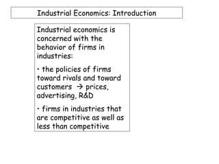
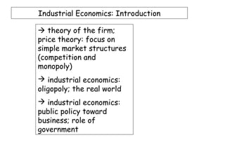
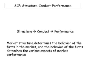
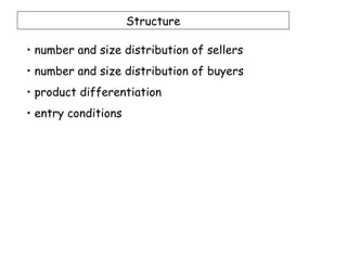
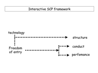
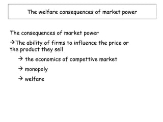
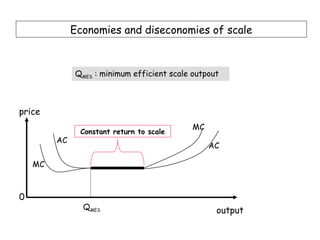
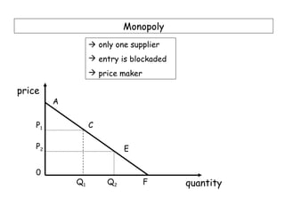
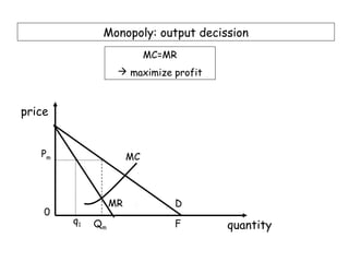
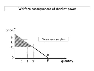
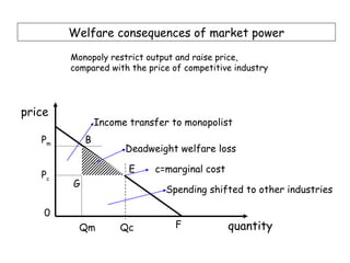
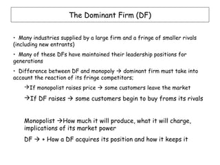
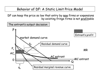
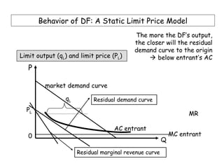
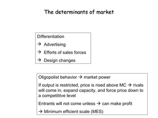
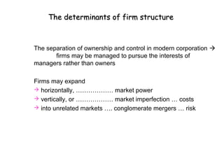
Industrial Economics: Introduction

Industrial economics is
concerned with the
behavior of firms in
industries:
• the policies of firms
toward rivals and toward
customers  prices,
advertising, R&D
• firms in industries that
are competitive as well as
less than competitive
Industrial Economics: Introduction

 theory of the firm;
price theory: focus on
simple market structures
(competition and
monopoly)
 industrial economics:
oligopoly; the real world
 industrial economics:
public policy toward
business; role of
government
SCP: Structure-Conduct-Performance


      Structure  Conduct  Performance


Market structure determines the behavior of the
firms in the market, and the behavior of the firms
detrmines the various aspects of market
performance
Structure

• number and size distribution of sellers
• number and size distribution of buyers
• product differentiation
• entry conditions
Conduct

• collusion
• strategic behavior
• advertising
• research and development
Performance

• profitability
• efficiency
• progressiveness
Interactive SCP framework


                progressiveness
                               profitability
technology
                 structure

                  strategy               perfomance

demand            conduct


                sales effort
Interactive SCP framework


technology
                                         structure

                                         conduct
Freedom
of entry
                                         perfomance
The welfare consequences of market power


The consequences of market power
The ability of firms to influence the price or
the product they sell
    the economics of compettive market
    monopoly
    welfare
Competition

Formal assumption of the competitive model:
• many small buyers and sellers
• standardized product
• free and easy entry and exit
• complete and perfect knowledge
Inputs and costs: fixed and variable

• fixed inputs  past investment decission
• variable inputs  level of output
• fixed costs  services of fixed factors
• variable costs  variable factors of production
        variable factor: labor
       fixed factor: capital
      opportunity cost, rental cost of capital services
       normal profit: (average cost-AVC)
       economic profit: (price-average cost)
Costs curves: typical firm & market

AC: average cost
AVC: average variable cost
MC: marginal cost
S1, S1   : short-run supply curves
D: demand curve
(qSD , pSD): shutdown point  minimizes losses
(qLR , pLR): long-run equilibrium for a typical firm
(QLR , PLR): market long-run equilibrium
Cost curves  under competition

      The firm’s supply decission: to maximize profit

       Firm is a price taker  choose the ouput that MC=P1  q1

                typical firm                            market
     price                MC

                               AC                            S1

P1                                  AVC                                 S2

PLR
PSD                                                                          D

             qSD qLR q1               firm              Q1        QLR        market
                                      output                                 output
Short-run and Long-run equilibrium: Competition

S1   : short-run supply curves
D: demand curve
           P1 : initial short-run equilibrium price
             Q1 : market output in the short-run

           q1 : firm’s output in the short-run equilibrium
Firm’s profit  economic profit  attract new firms
S1  S2

           PLR : long-run equilibrium price
             QLR : market output in the long-run

           qLR : firm’s output in the long-run equilibrium
Economies and diseconomies of scale


              QMES : minimum efficient scale outpout


price
                                             MC
               Constant return to scale
         AC
                                                  AC

    MC


0
                QMES                               output
Monopoly
                   only one supplier
                   entry is blockaded
                   price maker

price
         A


    P1            C

    P2                      E


    0
             Q1        Q2         F      quantity
Monopoly: output decission
                            MC=MR
                    maximize profit


price


   Pm                  MC


                  MR            D
    0
        q1   Qm                 F      quantity
Welfare consequences of market power


price

   P1
                      Consumers’ surplus
   P2
   P3


                          D
    0
         1   2   3        F          quantity
Welfare consequences of market power

        Monopoly restrict output and raise price,
        compared with the price of competitive industry


price
                Income transfer to monopolist
   Pm       B
                      Deadweight welfare loss

                       E    c=marginal cost
   Pc
        G
                               Spending shifted to other industries

    0
          Qm         Qc          F            quantity
The Dominant Firm (DF)


• Many industries supplied by a large firm and a fringe of smaller rivals
(including new entrants)
• Many of these DFs have maintained their leadership positions for
generations
• Difference between DF and monopoly  dominant firm must take into
account the reaction of its fringe competitors;
    If monopolist raises price  some customers leave the market
    If DF raises  some customers begin to buy froms its rivals


    Monopolist How much it will produce, what it will charge,
    implications of its market power
    DF  + How a DF acquires its position and how it keeps it
Behavior of DF: A Static Limit Price Model
DF can keep the price so low that entry by new firms or expansions
                          by existing fringe firms is not profitable

The entrant’s output decission

   P
                                                           Entrant’s profit
         market demand curve

                qd         Residual demand curve
   Pe
                                                                  MR
 ACe
                                  AC entrant
   0                                                       MC entrant
                                                       Q

        qe           Residual marginal revenue curve
Behavior of DF: A Static Limit Price Model
                                           The more the DF’s output,
                                           the closer will the residual
                                           demand curve to the origin
Limit output (qL) and limit price (PL)           below entrant’s AC
   P

         market demand curve

                 qL         Residual demand curve
  PL
                                                                  MR

                                   AC entrant
   0                                                        MC entrant
                                                        Q

                      Residual marginal revenue curve
A natural monopoly  government regulation
                               If the market is very small
                                 and entry costs are very
                                         high  it will not
Blockaded entry                profitable for new entrant
 P

       market demand curve


Pm
                                 AC entrant


                                            MC df
 0
                                        Q
             qm
Dynamic limit pricing


The static model ignores the fact that entry takes time  trade off
                                  between current and future profit


   the difference between the limit profit if it sets a low price
  and the larger short run profit if it sets a higher price
     the rate at which DF loses market share (profit) to the fringe if the
      fringe begins to expand
     the discount rate
Strategy to achieve and maintain dominance


Dominance is a power relation between two agents in which
the dominator restricts the action of the dominated
DF’s weapon: its output level which influence the price
DF is giving up the profit to maintain position
STRATEGIC BEHAVIOR:
      MERGER
      DIRECT COST-BASED STRATEGIES: increasing rival’s costs
    TECHNOLOGY-BASED STRATEGIES: capacity expansion, vertical
   integration
      MARKETING-BASED STRATEGIES: product differentiation, access
       to consumers
Summary

Firms may achieve a dominant position
 By superior competitive
performance
 By merger
 By strategic behavior design to
        exclude competitors and
prevent competition on the
merits


         PUBLIC POLICY
              toward
       DOMINANT FIRMS
Oligopoly: The recognition of interdependence


 Competititve market  each firm is so small  price taker
 Monopolist has no rival  price maker

 Dominant firm
    does consider the reaction of fringe firms  one sided
   recognition
    no recognition  if entry cost is low  give up mkt share
    fringe firms approach the size of DF  OLIGOPOLY


                                             supplied by few firms,
                      which recognize their mutual interdependence
Oligopoly: measuring fewness


 percentage of industry sales  the largest 4, the largest 10
 when the largest 4  40% of supply
     each must be aware of the others
     OLIGOPOLY


concentration ratio  summary index of fewness


 the Herfindahl Index
          combining information about market shares of all
firms in the market
Oligopoly: the decision making


 decide how much to produce
         let the market determine the price
         sunk cost

set the price
         sell whatever quantity demanded at that price
         the technology allows rapid changes in the rate of output
Oligopoly: the quantity-setting
                                     Cournot Duopoly
                                          a market supplied by
                                        two identical firms


P

     market demand curve

                     Residual demand curve


                     q2
                                                 MC = AC
                                             Q
                 Residual marginal
    q1(q2)       revenue curve
Oligopoly: the quantity-setting

                                            The ouput each firm will choose
                                depends on what it thinks the other firm will do

Firm’s 2 output
   qc
                          Firm’s 1 reaction curve

   qm
                   A
q2,A
                                       Firm’s 2 reaction curve
    q2’,B    B


                                                         Firm’s 1 output
            q1,A           qm         qc
Oligopoly: price-setting


 homogenous product
 differentiated product


 public policy toward oligopoly
         conspiracy to monopolize


                           COLLUSION
The determinants of market structure


3 faktor penting dalam struktur pasar
                  entry condition

 economies of scale
 product differentiation
 absolute cost advantages of existing firms
The determinants of market


          If there is economies of scale
      average cost falls as output increases

for constant MC = c
        C (q)   = F = cq
        AC(q) = c + (F/q)
Function coefficient: economies of scale
        FC = AC/MC = (c+(F/q)/c = 1 + F/cq


Economies of scale becomes more important as fixed
cost increases
Short-run equilibrium, n-firm Cournot oligopoly


      a
           market demand curve:    P=a-bQ

                          Residual demand curve
PSR
                                       AC=(F/q)+c
ACSR
                                                        MC = c
                                                    Q
              qSR              S

                      Residual marginal revenue
Short-run equilibrium, n-firm Cournot oligopoly


  Firm i’s MR
   Firm i’s revenue will change as firm i changes its output
          MRi = P + qi( ∆Pi/ ∆qi) = P-bqi = a – bQ – bqi
   maximizing profit by picking the output level that
          MR=MC atau a – bQ – bqi = c atau Q + qi = (a-c)/b
  a natural measure of market size = S = (a-c)/b
  All firms produce the same output in equilibrium: Q=Nq
   qSR = S/(n+1)
   PSR = c + (bS/(n+1))
Long-run equilibrium, Cournot oligopoly


               Residual demand curve

         a
             market demand curve:      P=a-bQ

                                                AC=(F/q)+c
PLR = ACLR

                                                     MC = c
                                                 Q
               qLR            S
Number of firms


In SR equilibrium, each firm earns a profit:
        ΠSR = b (S/(N+1))2 – F
the LR equilibrium number of firms  SR firm’s profit = 0
        nLR= (S/√(F/b)) – 1
number of firms ↓ ∼ market concentration ↑ ∼ fixed cost ↑


 The market ought to be more concentrated in the long
run, the greater the economies of large scale production
The determinants of market


Differentiation
 Advertising
 Efforts of sales forces
 Design changes


Oligopolist behavior  market power
If output is restricted, price is rised above MC  rivals
will come in, expand capacity, and force price down to
a competititve level
Entrants will not come unless  can make profit
 Minimum efficient scale (MES)
The determinants of firm structure


The separation of ownership and control in modern corporation 
       firms may be managed to pursue the interests of
managers rather than owners

Firms may expand
 horizontally, ……………… market power
 vertically, or ……………… market imperfection … costs
 into unrelated markets …. conglomerate mergers … risk

Ekonomi industri hands out

  • 1.
    Industrial Economics: Introduction Industrialeconomics is concerned with the behavior of firms in industries: • the policies of firms toward rivals and toward customers  prices, advertising, R&D • firms in industries that are competitive as well as less than competitive
  • 2.
    Industrial Economics: Introduction theory of the firm; price theory: focus on simple market structures (competition and monopoly)  industrial economics: oligopoly; the real world  industrial economics: public policy toward business; role of government
  • 3.
    SCP: Structure-Conduct-Performance Structure  Conduct  Performance Market structure determines the behavior of the firms in the market, and the behavior of the firms detrmines the various aspects of market performance
  • 4.
    Structure • number andsize distribution of sellers • number and size distribution of buyers • product differentiation • entry conditions
  • 5.
    Conduct • collusion • strategicbehavior • advertising • research and development
  • 6.
  • 7.
    Interactive SCP framework progressiveness profitability technology structure strategy perfomance demand conduct sales effort
  • 8.
    Interactive SCP framework technology structure conduct Freedom of entry perfomance
  • 9.
    The welfare consequencesof market power The consequences of market power The ability of firms to influence the price or the product they sell  the economics of compettive market  monopoly  welfare
  • 10.
    Competition Formal assumption ofthe competitive model: • many small buyers and sellers • standardized product • free and easy entry and exit • complete and perfect knowledge
  • 11.
    Inputs and costs:fixed and variable • fixed inputs  past investment decission • variable inputs  level of output • fixed costs  services of fixed factors • variable costs  variable factors of production  variable factor: labor  fixed factor: capital opportunity cost, rental cost of capital services  normal profit: (average cost-AVC)  economic profit: (price-average cost)
  • 12.
    Costs curves: typicalfirm & market AC: average cost AVC: average variable cost MC: marginal cost S1, S1 : short-run supply curves D: demand curve (qSD , pSD): shutdown point  minimizes losses (qLR , pLR): long-run equilibrium for a typical firm (QLR , PLR): market long-run equilibrium
  • 13.
    Cost curves under competition The firm’s supply decission: to maximize profit  Firm is a price taker  choose the ouput that MC=P1  q1 typical firm market price MC AC S1 P1 AVC S2 PLR PSD D qSD qLR q1 firm Q1 QLR market output output
  • 14.
    Short-run and Long-runequilibrium: Competition S1 : short-run supply curves D: demand curve  P1 : initial short-run equilibrium price  Q1 : market output in the short-run  q1 : firm’s output in the short-run equilibrium Firm’s profit  economic profit  attract new firms S1  S2  PLR : long-run equilibrium price  QLR : market output in the long-run  qLR : firm’s output in the long-run equilibrium
  • 15.
    Economies and diseconomiesof scale QMES : minimum efficient scale outpout price MC Constant return to scale AC AC MC 0 QMES output
  • 16.
    Monopoly  only one supplier  entry is blockaded  price maker price A P1 C P2 E 0 Q1 Q2 F quantity
  • 17.
    Monopoly: output decission MC=MR  maximize profit price Pm MC MR D 0 q1 Qm F quantity
  • 18.
    Welfare consequences ofmarket power price P1 Consumers’ surplus P2 P3 D 0 1 2 3 F quantity
  • 19.
    Welfare consequences ofmarket power Monopoly restrict output and raise price, compared with the price of competitive industry price Income transfer to monopolist Pm B Deadweight welfare loss E c=marginal cost Pc G Spending shifted to other industries 0 Qm Qc F quantity
  • 20.
    The Dominant Firm(DF) • Many industries supplied by a large firm and a fringe of smaller rivals (including new entrants) • Many of these DFs have maintained their leadership positions for generations • Difference between DF and monopoly  dominant firm must take into account the reaction of its fringe competitors; If monopolist raises price  some customers leave the market If DF raises  some customers begin to buy froms its rivals Monopolist How much it will produce, what it will charge, implications of its market power DF  + How a DF acquires its position and how it keeps it
  • 21.
    Behavior of DF:A Static Limit Price Model DF can keep the price so low that entry by new firms or expansions by existing fringe firms is not profitable The entrant’s output decission P Entrant’s profit market demand curve qd Residual demand curve Pe MR ACe AC entrant 0 MC entrant Q qe Residual marginal revenue curve
  • 22.
    Behavior of DF:A Static Limit Price Model The more the DF’s output, the closer will the residual demand curve to the origin Limit output (qL) and limit price (PL)  below entrant’s AC P market demand curve qL Residual demand curve PL MR AC entrant 0 MC entrant Q Residual marginal revenue curve
  • 23.
    A natural monopoly government regulation If the market is very small and entry costs are very high  it will not Blockaded entry profitable for new entrant P market demand curve Pm AC entrant MC df 0 Q qm
  • 24.
    Dynamic limit pricing Thestatic model ignores the fact that entry takes time  trade off between current and future profit  the difference between the limit profit if it sets a low price and the larger short run profit if it sets a higher price  the rate at which DF loses market share (profit) to the fringe if the fringe begins to expand  the discount rate
  • 25.
    Strategy to achieveand maintain dominance Dominance is a power relation between two agents in which the dominator restricts the action of the dominated DF’s weapon: its output level which influence the price DF is giving up the profit to maintain position STRATEGIC BEHAVIOR:  MERGER  DIRECT COST-BASED STRATEGIES: increasing rival’s costs  TECHNOLOGY-BASED STRATEGIES: capacity expansion, vertical integration  MARKETING-BASED STRATEGIES: product differentiation, access to consumers
  • 26.
    Summary Firms may achievea dominant position  By superior competitive performance  By merger  By strategic behavior design to exclude competitors and prevent competition on the merits PUBLIC POLICY toward DOMINANT FIRMS
  • 27.
    Oligopoly: The recognitionof interdependence  Competititve market  each firm is so small  price taker  Monopolist has no rival  price maker  Dominant firm  does consider the reaction of fringe firms  one sided recognition  no recognition  if entry cost is low  give up mkt share  fringe firms approach the size of DF  OLIGOPOLY supplied by few firms, which recognize their mutual interdependence
  • 28.
    Oligopoly: measuring fewness percentage of industry sales  the largest 4, the largest 10  when the largest 4  40% of supply  each must be aware of the others  OLIGOPOLY concentration ratio  summary index of fewness  the Herfindahl Index  combining information about market shares of all firms in the market
  • 29.
    Oligopoly: the decisionmaking  decide how much to produce  let the market determine the price  sunk cost set the price  sell whatever quantity demanded at that price  the technology allows rapid changes in the rate of output
  • 30.
    Oligopoly: the quantity-setting Cournot Duopoly  a market supplied by two identical firms P market demand curve Residual demand curve q2 MC = AC Q Residual marginal q1(q2) revenue curve
  • 31.
    Oligopoly: the quantity-setting The ouput each firm will choose depends on what it thinks the other firm will do Firm’s 2 output qc Firm’s 1 reaction curve qm A q2,A Firm’s 2 reaction curve q2’,B B Firm’s 1 output q1,A qm qc
  • 32.
    Oligopoly: price-setting  homogenousproduct  differentiated product  public policy toward oligopoly  conspiracy to monopolize COLLUSION
  • 33.
    The determinants ofmarket structure 3 faktor penting dalam struktur pasar  entry condition  economies of scale  product differentiation  absolute cost advantages of existing firms
  • 34.
    The determinants ofmarket If there is economies of scale  average cost falls as output increases for constant MC = c C (q) = F = cq AC(q) = c + (F/q) Function coefficient: economies of scale FC = AC/MC = (c+(F/q)/c = 1 + F/cq Economies of scale becomes more important as fixed cost increases
  • 35.
    Short-run equilibrium, n-firmCournot oligopoly a market demand curve: P=a-bQ Residual demand curve PSR AC=(F/q)+c ACSR MC = c Q qSR S Residual marginal revenue
  • 36.
    Short-run equilibrium, n-firmCournot oligopoly Firm i’s MR  Firm i’s revenue will change as firm i changes its output MRi = P + qi( ∆Pi/ ∆qi) = P-bqi = a – bQ – bqi maximizing profit by picking the output level that MR=MC atau a – bQ – bqi = c atau Q + qi = (a-c)/b a natural measure of market size = S = (a-c)/b All firms produce the same output in equilibrium: Q=Nq  qSR = S/(n+1)  PSR = c + (bS/(n+1))
  • 37.
    Long-run equilibrium, Cournotoligopoly Residual demand curve a market demand curve: P=a-bQ AC=(F/q)+c PLR = ACLR MC = c Q qLR S
  • 38.
    Number of firms InSR equilibrium, each firm earns a profit: ΠSR = b (S/(N+1))2 – F the LR equilibrium number of firms  SR firm’s profit = 0 nLR= (S/√(F/b)) – 1 number of firms ↓ ∼ market concentration ↑ ∼ fixed cost ↑  The market ought to be more concentrated in the long run, the greater the economies of large scale production
  • 39.
    The determinants ofmarket Differentiation  Advertising  Efforts of sales forces  Design changes Oligopolist behavior  market power If output is restricted, price is rised above MC  rivals will come in, expand capacity, and force price down to a competititve level Entrants will not come unless  can make profit  Minimum efficient scale (MES)
  • 40.
    The determinants offirm structure The separation of ownership and control in modern corporation  firms may be managed to pursue the interests of managers rather than owners Firms may expand  horizontally, ……………… market power  vertically, or ……………… market imperfection … costs  into unrelated markets …. conglomerate mergers … risk