Download to read offline


![Intro Model Equilibrium E¢ ciency Frictionless Implications Policy Examples Conclusion Appx.
The model
A trading session in continuous time, t 2 [0, T], τ T t
Unit measure of banks hold reserve balances k (τ) 2 f0, 1, 2g
fnk (τ)g : distribution of balances at time T τ
Linear payo¤s from balances, discount at rate r
Uk : payo¤ from holding balance k at the end of the session
Trade opportunities are bilateral and random (Poisson rate α)
Loan and repayment amounts determined by Nash bargaining
Assume all loans repaid at time T + ∆, where ∆ 2 R+](https://image.slidesharecdn.com/economicsslides-161007195739/85/Economicsslides-10-320.jpg)


![Intro Model Equilibrium E¢ ciency Frictionless Implications Policy Examples Conclusion Appx.
Institutional features of the fed funds market
Model Fed funds market
Search and bargaining Over-the-counter market
[0, T]](https://image.slidesharecdn.com/economicsslides-161007195739/85/Economicsslides-13-320.jpg)
![Intro Model Equilibrium E¢ ciency Frictionless Implications Policy Examples Conclusion Appx.
Institutional features of the fed funds market
Model Fed funds market
Search and bargaining Over-the-counter market
[0, T] 4:00pm-6:30pm](https://image.slidesharecdn.com/economicsslides-161007195739/85/Economicsslides-14-320.jpg)
![Intro Model Equilibrium E¢ ciency Frictionless Implications Policy Examples Conclusion Appx.
Institutional features of the fed funds market
Model Fed funds market
Search and bargaining Over-the-counter market
[0, T] 4:00pm-6:30pm
fnk (T)g](https://image.slidesharecdn.com/economicsslides-161007195739/85/Economicsslides-15-320.jpg)
![Intro Model Equilibrium E¢ ciency Frictionless Implications Policy Examples Conclusion Appx.
Institutional features of the fed funds market
Model Fed funds market
Search and bargaining Over-the-counter market
[0, T] 4:00pm-6:30pm
fnk (T)g
Distribution of reserve
balances at 4:00pm](https://image.slidesharecdn.com/economicsslides-161007195739/85/Economicsslides-16-320.jpg)
![Intro Model Equilibrium E¢ ciency Frictionless Implications Policy Examples Conclusion Appx.
Institutional features of the fed funds market
Model Fed funds market
Search and bargaining Over-the-counter market
[0, T] 4:00pm-6:30pm
fnk (T)g
Distribution of reserve
balances at 4:00pm
fUk g](https://image.slidesharecdn.com/economicsslides-161007195739/85/Economicsslides-17-320.jpg)
![Intro Model Equilibrium E¢ ciency Frictionless Implications Policy Examples Conclusion Appx.
Institutional features of the fed funds market
Model Fed funds market
Search and bargaining Over-the-counter market
[0, T] 4:00pm-6:30pm
fnk (T)g
Distribution of reserve
balances at 4:00pm
fUk g Reserve requirements,
interest on reserves...](https://image.slidesharecdn.com/economicsslides-161007195739/85/Economicsslides-18-320.jpg)

![Intro Model Equilibrium E¢ ciency Frictionless Implications Policy Examples Conclusion Appx.
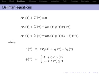
Bellman equations
rV1 (τ) + ˙V1 (τ) = 0
rV0 (τ) + ˙V0 (τ) = αn2 (τ) max fV1 (τ) V0 (τ) ¯R (τ) , 0g
rV2 (τ) + ˙V2 (τ) = αn0 (τ) max fV1 (τ) V2 (τ) + ¯R (τ) , 0g
Vk (0) = Uk
¯R (τ) = arg max
R
[V1 (τ) R V0 (τ)]θ
[V1 (τ) + R V2 (τ)]1 θ
= θ [V2 (τ) V1 (τ)] + (1 θ) [V1 (τ) V0 (τ)]
¯R (τ) e r(τ+∆)
R (τ) (PDV of repayment)](https://image.slidesharecdn.com/economicsslides-161007195739/85/Economicsslides-20-320.jpg)
![Intro Model Equilibrium E¢ ciency Frictionless Implications Policy Examples Conclusion Appx.
Analysis
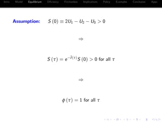
˙S (τ) = δ (τ) S (τ)
δ (τ) fr + αφ (τ) [θn2 (τ) + (1 θ) n0 (τ)]g
)
S (τ) = e
¯δ(τ)
S (0)
¯δ (τ)
Z τ
0
δ (x) dx
S (τ) 2V1 (τ) V0 (τ) V2 (τ)](https://image.slidesharecdn.com/economicsslides-161007195739/85/Economicsslides-24-320.jpg)
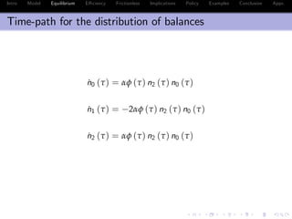
![Intro Model Equilibrium E¢ ciency Frictionless Implications Policy Examples Conclusion Appx.
Analysis
˙S (τ) = δ (τ) S (τ)
δ (τ) fr + αφ (τ) [θn2 (τ) + (1 θ) n0 (τ)]g
)
S (τ) = e
¯δ(τ)
S (0)
¯δ (τ)
Z τ
0
δ (x) dx
S (τ) 2V1 (τ) V0 (τ) V2 (τ)](https://image.slidesharecdn.com/economicsslides-161007195739/85/Economicsslides-25-320.jpg)


![Intro Model Equilibrium E¢ ciency Frictionless Implications Policy Examples Conclusion Appx.
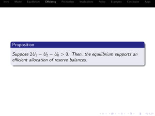
Proposition
Suppose 2U1 U2 U0 > 0. Then the unique equilibrium is:
n2 (τ) = n0 (τ) + n2 (T) n0 (T)
n1 (τ) = 1 2n0 (τ) + n0 (T) n2 (T)
n0 (τ) = [n2(T ) n0(T )]n0(T )
eα[n2(T ) n0(T )](T τ)n2(T ) n0(T )
S (τ) =
[n2(T ) e α[n2(T ) n0(T )](T τ)n0(T )]e fr+αθ[n2(T ) n0(T )]gτ
n2(T ) e α[n2(T ) n0(T )]T n0(T )
S (0)
R (τ) = er∆
fβ (τ) (U2 U1) + [1 β (τ)] (U1 U0)g
β (τ)
θ[n2(T ) e α[n2(T ) n0(T )](T τ)n0(T )]e αθ[n2(T ) n0(T )]τ
n2(T ) e α[n2(T ) n0(T )]T n0(T )
+
[1 e αθ[n2(T ) n0(T )]τ
]n2(T )
n2(T ) e α[n2(T ) n0(T )]T n0(T )](https://image.slidesharecdn.com/economicsslides-161007195739/85/Economicsslides-29-320.jpg)
![Intro Model Equilibrium E¢ ciency Frictionless Implications Policy Examples Conclusion Appx.
Proposition
Suppose 2U1 U2 U0 > 0. Then the unique equilibrium is:
n2 (τ) = n0 (τ) + n2 (T) n0 (T)
n1 (τ) = 1 2n0 (τ) + n0 (T) n2 (T)
n0 (τ) = [n2(T ) n0(T )]n0(T )
eα[n2(T ) n0(T )](T τ)n2(T ) n0(T )
S (τ) =
[n2(T ) e α[n2(T ) n0(T )](T τ)n0(T )]e fr+αθ[n2(T ) n0(T )]gτ
n2(T ) e α[n2(T ) n0(T )]T n0(T )
S (0)
R (τ) = er∆
fβ (τ) (U2 U1) + [1 β (τ)] (U1 U0)g
β (τ)
θ[n2(T ) e α[n2(T ) n0(T )](T τ)n0(T )]e αθ[n2(T ) n0(T )]τ
n2(T ) e α[n2(T ) n0(T )]T n0(T )
+
[1 e αθ[n2(T ) n0(T )]τ
]n2(T )
n2(T ) e α[n2(T ) n0(T )]T n0(T )](https://image.slidesharecdn.com/economicsslides-161007195739/85/Economicsslides-30-320.jpg)
![Intro Model Equilibrium E¢ ciency Frictionless Implications Policy Examples Conclusion Appx.
Proposition
Suppose 2U1 U2 U0 > 0. Then the unique equilibrium is:
n2 (τ) = n0 (τ) + n2 (T) n0 (T)
n1 (τ) = 1 2n0 (τ) + n0 (T) n2 (T)
n0 (τ) = [n2(T ) n0(T )]n0(T )
eα[n2(T ) n0(T )](T τ)n2(T ) n0(T )
S (τ) =
[n2(T ) e α[n2(T ) n0(T )](T τ)n0(T )]e fr+αθ[n2(T ) n0(T )]gτ
n2(T ) e α[n2(T ) n0(T )]T n0(T )
S (0)
R (τ) = er∆
fβ (τ) (U2 U1) + [1 β (τ)] (U1 U0)g
β (τ)
θ[n2(T ) e α[n2(T ) n0(T )](T τ)n0(T )]e αθ[n2(T ) n0(T )]τ
n2(T ) e α[n2(T ) n0(T )]T n0(T )
+
[1 e αθ[n2(T ) n0(T )]τ
]n2(T )
n2(T ) e α[n2(T ) n0(T )]T n0(T )](https://image.slidesharecdn.com/economicsslides-161007195739/85/Economicsslides-31-320.jpg)
![Intro Model Equilibrium E¢ ciency Frictionless Implications Policy Examples Conclusion Appx.
Proposition
Suppose 2U1 U2 U0 > 0. Then the unique equilibrium is:
n2 (τ) = n0 (τ) + n2 (T) n0 (T)
n1 (τ) = 1 2n0 (τ) + n0 (T) n2 (T)
n0 (τ) = [n2(T ) n0(T )]n0(T )
eα[n2(T ) n0(T )](T τ)n2(T ) n0(T )
S (τ) =
[n2(T ) e α[n2(T ) n0(T )](T τ)n0(T )]e fr+αθ[n2(T ) n0(T )]gτ
n2(T ) e α[n2(T ) n0(T )]T n0(T )
S (0)
R (τ) = er∆
fβ (τ) (U2 U1) + [1 β (τ)] (U1 U0)g
β (τ)
θ[n2(T ) e α[n2(T ) n0(T )](T τ)n0(T )]e αθ[n2(T ) n0(T )]τ
n2(T ) e α[n2(T ) n0(T )]T n0(T )
+
[1 e αθ[n2(T ) n0(T )]τ
]n2(T )
n2(T ) e α[n2(T ) n0(T )]T n0(T )](https://image.slidesharecdn.com/economicsslides-161007195739/85/Economicsslides-32-320.jpg)
![Intro Model Equilibrium E¢ ciency Frictionless Implications Policy Examples Conclusion Appx.
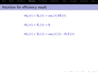
Intuition for e¢ ciency result
rV0 (τ) + ˙V0 (τ) = αn2 (τ) θS (τ)
rλ0 (τ) + ˙λ0 (τ) = αn2 (τ) S (τ)
rV1 (τ) + ˙V1 (τ) = 0
rλ1 (τ) + ˙λ1 (τ) = 0
rV2 (τ) + ˙V2 (τ) = αn0 (τ) (1 θ) S (τ)
rλ2 (τ) + ˙λ2 (τ) = αn0 (τ) S (τ)
S (τ) = e
¯δ(τ)
S (0)
S (τ) = e
¯δ (τ)
S (0)
¯δ (τ) ¯δ (τ) = α
Z τ
0
[(1 θ) n2 (z) + θn0 (z)] dz 0](https://image.slidesharecdn.com/economicsslides-161007195739/85/Economicsslides-35-320.jpg)
![Intro Model Equilibrium E¢ ciency Frictionless Implications Policy Examples Conclusion Appx.
Intuition for e¢ ciency result
rV0 (τ) + ˙V0 (τ) = αn2 (τ) θS (τ)
rλ0 (τ) + ˙λ0 (τ) = αn2 (τ) S (τ)
rV1 (τ) + ˙V1 (τ) = 0
rλ1 (τ) + ˙λ1 (τ) = 0
rV2 (τ) + ˙V2 (τ) = αn0 (τ) (1 θ) S (τ)
rλ2 (τ) + ˙λ2 (τ) = αn0 (τ) S (τ)
S (τ) = e
¯δ(τ)
S (0)
S (τ) = e
¯δ (τ)
S (0)
¯δ (τ) ¯δ (τ) = α
Z τ
0
[(1 θ) n2 (z) + θn0 (z)] dz 0](https://image.slidesharecdn.com/economicsslides-161007195739/85/Economicsslides-36-320.jpg)
![Intro Model Equilibrium E¢ ciency Frictionless Implications Policy Examples Conclusion Appx.
Intuition for e¢ ciency result
rV0 (τ) + ˙V0 (τ) = αn2 (τ) θS (τ)
rλ0 (τ) + ˙λ0 (τ) = αn2 (τ) S (τ)
rV1 (τ) + ˙V1 (τ) = 0
rλ1 (τ) + ˙λ1 (τ) = 0
rV2 (τ) + ˙V2 (τ) = αn0 (τ) (1 θ) S (τ)
rλ2 (τ) + ˙λ2 (τ) = αn0 (τ) S (τ)
S (τ) = e
¯δ(τ)
S (0)
S (τ) = e
¯δ (τ)
S (0)
¯δ (τ) ¯δ (τ) = α
Z τ
0
[(1 θ) n2 (z) + θn0 (z)] dz 0](https://image.slidesharecdn.com/economicsslides-161007195739/85/Economicsslides-37-320.jpg)
![Intro Model Equilibrium E¢ ciency Frictionless Implications Policy Examples Conclusion Appx.
Intuition for e¢ ciency result
Equilibrium:
Gain from trade as perceived by borrower: θS (τ)
Gain from trade as perceived by lender: (1 θ) S (τ)
Planner:
Each of their marginal contributions equals S (τ)
δ (τ) δ (τ) for all τ 2 [0, T], with “=” only for τ = 0
) The planner “discounts”more heavily than the equilibrium
) S (τ) < S (τ) for all τ 2 (0, 1]
) Social value of loan < joint private value of loan](https://image.slidesharecdn.com/economicsslides-161007195739/85/Economicsslides-38-320.jpg)
![Intro Model Equilibrium E¢ ciency Frictionless Implications Policy Examples Conclusion Appx.
Intuition for e¢ ciency result
Equilibrium:
Gain from trade as perceived by borrower: θS (τ)
Gain from trade as perceived by lender: (1 θ) S (τ)
Planner:
Each of their marginal contributions equals S (τ)
δ (τ) δ (τ) for all τ 2 [0, T], with “=” only for τ = 0
) The planner “discounts”more heavily than the equilibrium
) S (τ) < S (τ) for all τ 2 (0, 1]
) Social value of loan < joint private value of loan](https://image.slidesharecdn.com/economicsslides-161007195739/85/Economicsslides-39-320.jpg)
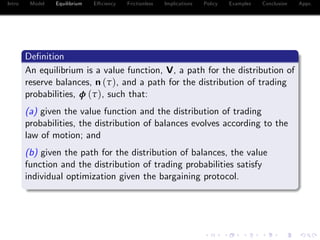
![Intro Model Equilibrium E¢ ciency Frictionless Implications Policy Examples Conclusion Appx.
Intuition for e¢ ciency result
Equilibrium:
Gain from trade as perceived by borrower: θS (τ)
Gain from trade as perceived by lender: (1 θ) S (τ)
Planner:
Each of their marginal contributions equals S (τ)
δ (τ) δ (τ) for all τ 2 [0, T], with “=” only for τ = 0
) The planner “discounts”more heavily than the equilibrium
) S (τ) < S (τ) for all τ 2 (0, 1]
) Social value of loan < joint private value of loan](https://image.slidesharecdn.com/economicsslides-161007195739/85/Economicsslides-40-320.jpg)
![Intro Model Equilibrium E¢ ciency Frictionless Implications Policy Examples Conclusion Appx.
Intuition for e¢ ciency result
Equilibrium:
Gain from trade as perceived by borrower: θS (τ)
Gain from trade as perceived by lender: (1 θ) S (τ)
Planner:
Each of their marginal contributions equals S (τ)
δ (τ) δ (τ) for all τ 2 [0, T], with “=” only for τ = 0
) The planner “discounts”more heavily than the equilibrium
) S (τ) < S (τ) for all τ 2 (0, 1]
) Social value of loan < joint private value of loan](https://image.slidesharecdn.com/economicsslides-161007195739/85/Economicsslides-41-320.jpg)
![Intro Model Equilibrium E¢ ciency Frictionless Implications Policy Examples Conclusion Appx.
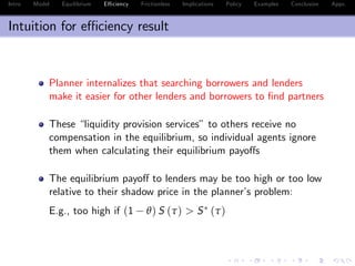
Intuition for e¢ ciency result
Equilibrium:
Gain from trade as perceived by borrower: θS (τ)
Gain from trade as perceived by lender: (1 θ) S (τ)
Planner:
Each of their marginal contributions equals S (τ)
δ (τ) δ (τ) for all τ 2 [0, T], with “=” only for τ = 0
) The planner “discounts”more heavily than the equilibrium
) S (τ) < S (τ) for all τ 2 (0, 1]
) Social value of loan < joint private value of loan](https://image.slidesharecdn.com/economicsslides-161007195739/85/Economicsslides-42-320.jpg)
![Intro Model Equilibrium E¢ ciency Frictionless Implications Policy Examples Conclusion Appx.
Intuition for e¢ ciency result
Equilibrium:
Gain from trade as perceived by borrower: θS (τ)
Gain from trade as perceived by lender: (1 θ) S (τ)
Planner:
Each of their marginal contributions equals S (τ)
δ (τ) δ (τ) for all τ 2 [0, T], with “=” only for τ = 0
) The planner “discounts”more heavily than the equilibrium
) S (τ) < S (τ) for all τ 2 (0, 1]
) Social value of loan < joint private value of loan](https://image.slidesharecdn.com/economicsslides-161007195739/85/Economicsslides-43-320.jpg)


![Intro Model Equilibrium E¢ ciency Frictionless Implications Policy Examples Conclusion Appx.
Frictionless limit
Proposition
Let Q ∑2
k=0 knk (T) = 1 + n2 (T) n0 (T).
For τ 2 [0, T], as α ! ∞, ρ (τ) ! ρ∞, where
1 + ρ∞
=
8
<
:
er∆
(U1 U0) if Q < 1
er∆
[θ (U2 U1) + (1 θ) (U1 U0)] if Q = 1
er∆
(U2 U1) if 1 < Q.](https://image.slidesharecdn.com/economicsslides-161007195739/85/Economicsslides-47-320.jpg)


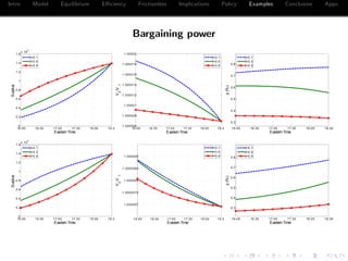
![Intro Model Equilibrium E¢ ciency Frictionless Implications Policy Examples Conclusion Appx.
Fed funds rate
The gross rate on a loan at time T τ is:
1 + ρ (τ) = er∆
fβ (τ) (U2 U1) + [1 β (τ)] (U1 U0)g
with
β (τ) 2 [0, 1]
The average daily rate is:
¯ρ =
1
T
Z T
0
ρ (τ) dτ](https://image.slidesharecdn.com/economicsslides-161007195739/85/Economicsslides-50-320.jpg)
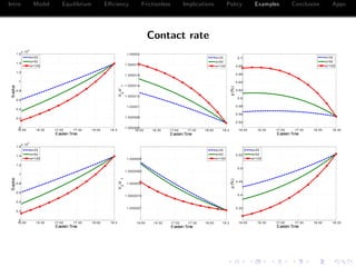
![Intro Model Equilibrium E¢ ciency Frictionless Implications Policy Examples Conclusion Appx.
Cross-sectional distribution of reserve balances
Let µ (τ) and σ2
(τ) denote the mean and variance of the
cross-sectional distribution of reserve balances at t = T τ
µ (τ) = 1 + n2 (T) n0 (T) Q
σ2
(τ) = σ2
(T) 2 [2 + n2 (T) n0 (T)] [n0 (T) n0 (τ)]](https://image.slidesharecdn.com/economicsslides-161007195739/85/Economicsslides-51-320.jpg)

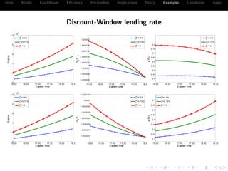
![Intro Model Equilibrium E¢ ciency Frictionless Implications Policy Examples Conclusion Appx.
U1 = e r∆
(1 + ir
f )
U2 = e r∆
(2 + ir
f + ie
f )
U0 = e r∆
(iw
f ir
f + Pw
)
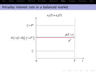
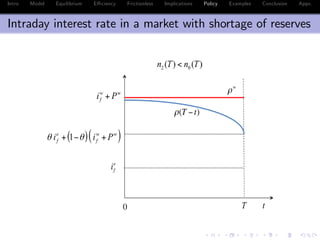
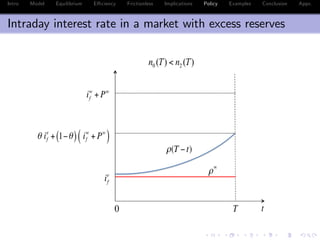
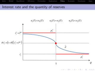
Proposition
ρ (τ) = β (τ) ie
f + [1 β (τ)] (iw
f + Pw
) where
1 If n2 (T) = n0 (T), β (τ) = θ
2 If n2 (T) < n0 (T), β (τ) 2 [0, θ], β (0) = θ and β0
(τ) < 0
3 If n0 (T) < n2 (T), β (τ) 2 [θ, 1], β (0) = θ and β0
(τ) > 0.](https://image.slidesharecdn.com/economicsslides-161007195739/85/Economicsslides-53-320.jpg)


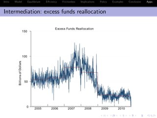
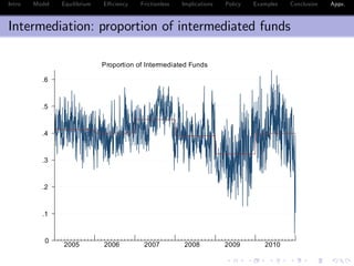


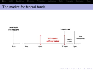
This document presents a model of the over-the-counter federal funds market. It uses a search-and-bargaining framework to model how banks with reserve shortages and surpluses are matched to reallocate balances. The model shows the fed funds rate is determined by banks' discount rates and the distribution of reserve balances held by banks. It also shows under certain conditions, the market structure achieves efficient reallocation of funds among banks.