Prepared By Brock Williams
Chapter 6
Market Efficiency
and Government
Intervention
The housing market in New York
City is highly regulated. The city
issues a relatively small number of
permits for new condominium
buildings, and rapid growth in the
demand for condominiums has
resulted in soaring condominium
prices.
Copyright ©2014 Pearson Education, Inc. All rights reserved. 6-2
Learning Objectives
1. Use demand and supply curves to compute
the value of markets
2. Explain why the market equilibrium
maximizes the value of a market
3. Describe the market effects of price
controls
4. Describe the market effects of quantity
controls
5. Explain how a tax is shifted to consumers
and input suppliers
Copyright ©2014 Pearson Education, Inc. All rights reserved. 6-3
● efficiency
A situation in which people do the best
they can, given their limited resources.
A market equilibrium will generate the largest possible surplus when four conditions
are met:
• No external benefits: The benefits of a product (a good or service) are confined
to the person who pays for it.
• No external costs: The cost of producing a product is confined to the person
who sells it.
• Perfect information: Buyers and sellers know enough about the product to make
informed decisions about whether to buy or sell it.
• Perfect competition: Each firm produces such a small quantity that the firm
cannot affect the price.
P R I N C I P L E O F V O L U N T A R Y E X C H A N G E
A voluntary exchange between two people makes both people better off.
Market Efficiency and
Government Intervention
Copyright ©2014 Pearson Education, Inc. All rights reserved. 6-4
● willingness to pay
The maximum amount a
consumer is willing to pay for a
product.
The Demand Curve and Consumer Surplus
● consumer surplus
The amount a consumer is willing
to pay for a product minus the
price the consumer actually pays.
6.1 CONSUMER SURPLUS AND
PRODUCER SURPLUS
Copyright ©2014 Pearson Education, Inc. All rights reserved. 6-5
The Demand Curve and Consumer Surplus
► FIGURE 6.1
The Demand Curve and
Consumer Surplus
Consumer surplus equals the
maximum amount a consumer is
willing to pay (shown by the
demand curve) minus the price
paid.
Juan is willing to pay $22, so if
the price is $10, his consumer
surplus is $12. The market
consumer surplus equals the
sum of the surpluses earned by
all consumers in the market. In
this case, the market consumer
surplus is $30 = $12 + $9 + $6 +
$3 + $0.
6.1 CONSUMER SURPLUS AND
PRODUCER SURPLUS (cont.)
Copyright ©2014 Pearson Education, Inc. All rights reserved. 6-6
The Supply Curve and Producer Surplus
● willingness to accept
The minimum amount a producer
is willing to accept as payment for
a product; equal to the marginal
cost of production.
● producer surplus
The price a producer receives for
a product minus the marginal cost
of production.
6.1 CONSUMER SURPLUS AND
PRODUCER SURPLUS (cont.)
Copyright ©2014 Pearson Education, Inc. All rights reserved. 6-7
The Supply Curve and Producer Surplus
 FIGURE 6.2
The Supply Curve and Producer Surplus
Producer surplus equals the market price minus the producer’s willingness to accept, or marginal cost
(shown by the supply curve).
Abe’s marginal cost is $2, so if the price is $10, his producer surplus is $8. The market producer
surplus equals the sum of the surpluses earned by all producers in the market. In this case, the
market producer surplus is $20 = $8 + $6 + $4 + $2 + $0.
6.1 CONSUMER SURPLUS AND
PRODUCER SURPLUS (cont.)
Copyright ©2014 Pearson Education, Inc. All rights reserved. 6-8
• What is the consumer surplus from Internet service? Two recent studies
compute consumers’ willingness to pay for Internet service. For Japanese
consumers, the average willingness to pay for Internet service (email and web
browsing delivered over personal computers) is $5,623 per month, compared to
an average price of broadband Internet service of $4,000.
• In other words, the average consumer surplus is $1,623, or about 40 percent of
the price.
• For US consumers, the average willingness to pay for Internet service is $85
per month, and with an average monthly price of $40, the consumer surplus is
$45 per month.
COMPUTER SURPLUS OF INTERNET SERICES
APPLYING THE CONCEPTS #1: How do we compute
consumer surplus?
A P P L I C A T I O N 1
Copyright ©2014 Pearson Education, Inc. All rights reserved. 6-9
 FIGURE 6.3
Market Equilibrium and the
Total Market Surplus
The total surplus of the market
equals consumer surplus (the
lightly shaded areas) plus
producer surplus (the darkly
shaded areas).
The market equilibrium
generates the highest possible
total market value, equal to
$50 = $30 (consumer surplus)
+ $20 (producer surplus).
● total surplus
The sum of consumer surplus and producer surplus.
6.2 MARKET EQUILIBRIUM AND
EFFICIENCY
Copyright ©2014 Pearson Education, Inc. All rights reserved. 6-10
Total Surplus Is Lower with a Price below the Equilibrium Price
● price ceiling
A maximum price set by the government.
Total Surplus Is Lower with a Price above the Equilibrium Price
● price floor
A minimum price set by the government.
6.2 MARKET EQUILIBRIUM AND
EFFICIENCY (cont.)
Copyright ©2014 Pearson Education, Inc. All rights reserved. 6-11
Total Surplus Is Lower with a Price above the Equilibrium Price
 FIGURE 6.4
Price Controls Decrease the Total Surplus of the Market
(A) A maximum price of $4 reduces the total surplus of the market. The first two consumers gain at the
expense of the first two producers. The consumer and producer surpluses for the third and fourth lawns are
lost entirely, so the total value of the market decreases.
(B) A minimum price of $19 reduces the total surplus of the market. The first two producers gain at the
expense of the first two consumers. The consumer and producer surpluses for the third and fourth lawns are
lost entirely, so the total value of the market decreases.
6.2 MARKET EQUILIBRIUM AND
EFFICIENCY (cont.)
Copyright ©2014 Pearson Education, Inc. All rights reserved. 6-12
Efficiency and the Invisible Hand
The market equilibrium maximizes the total surplus of the market because it
guarantees that all mutually beneficial transactions will happen.
Instead of using a bureaucrat to coordinate the actions of everyone in the
market, we can rely on the actions of individual consumers and individual
producers, each guided only by self-interest. This is Adam Smith’s invisible hand
in action.
In most modern economies, governments take an active role.
For a market that meets the four efficiency conditions, the market equilibrium
generates the largest possible total surplus, so government intervention can only
decrease the surplus and cause inefficiency.
Government Intervention in Efficient Markets
6.2 MARKET EQUILIBRIUM AND
EFFICIENCY (cont.)
Copyright ©2014 Pearson Education, Inc. All rights reserved. 6-13
• Under rent control, the government sets a maximum price for housing, decreasing
the quantity supplied and the total value of the market. Rent control and other
maximum prices cause inefficiency of another sort.
• Consider a consumer living in a rent-controlled apartment who experiences a change
in circumstances that would normally cause the consumer to a move to a different
apartment. For example, when a single person renting a tiny apartment gets
married, he or she is likely to move to a larger place. But a consumer in a rent-
controlled apartment may stay in the tiny but inexpensive apartment, generating a
housing mismatch. A recent study suggests that in New York City, about 20 percent
of rent-controlled apartments are mismatched.
• The most famous case of a mismatched tenant is former Mayor Koch of New York.
When he was elected mayor and moved into the mayor’s official residence, he held
onto his rent-controlled apartment, presumably anticipating his post-mayor life in an
apartment at a controlled rent that was roughly one-third the market rent.
RENT CONTROL AND MISMATCHES
APPLYING THE CONCEPTS #2: Why does the
market equilibrium maximize the value of a
market?
A P P L I C A T I O N 2
Copyright ©2014 Pearson Education, Inc. All rights reserved. 6-14
Setting Maximum Prices
Here are some examples of goods that have been subject to maximum prices or
may be subject to maximum prices in the near future:
• Rental housing.
• Gasoline.
• Medical goods and services.
In all three cases, a maximum price will cause excess demand and reduce the
total surplus of the market.
6.3 CONTROLLING PRICES—MAXIMUM
AND MINIMUM PRICES
Copyright ©2014 Pearson Education, Inc. All rights reserved. 6-15
Rent Control  FIGURE 6.5
Rent Control
Decreases Total
Surplus
(A) In the market
equilibrium, with a price
of $400 and 1,000
apartments, the total
surplus is the area
between the demand
curve and the supply
curve.
(B) Rent control, with a
maximum price of
$300, reduces the
quantity to 700
apartments and
decreases the total
surplus.● deadweight loss
The decrease in the total surplus of the market
that results from a policy such as rent control.
6.3 CONTROLLING PRICES—MAXIMUM
AND MINIMUM PRICES (cont.)
Copyright ©2014 Pearson Education, Inc. All rights reserved. 6-16
Rent Control
Because rent control outlaws transactions that would make both parties better
off, it causes inefficiency.
Three more subtle effects associated with rent control add to its inefficiency:
• Search costs.
• Cheating.
• Decrease in quality of housing.
P R I N C I P L E O F V O L U N T A R Y E X C H A N G E
A voluntary exchange between two people makes both people better off.
6.3 CONTROLLING PRICES—MAXIMUM
AND MINIMUM PRICES (cont.)
Copyright ©2014 Pearson Education, Inc. All rights reserved. 6-17
Setting Minimum Prices
• Recall that when government sets a minimum price above the
equilibrium price, the result is permanent excess supply.
• Governments around the world establish minimum prices for
agricultural goods.
• Under a price-support program, a government sets a minimum
price for an agricultural product and then buys any resulting
surpluses at that price.
6.3 CONTROLLING PRICES—MAXIMUM
AND MINIMUM PRICES (cont.)
Copyright ©2014 Pearson Education, Inc. All rights reserved. 6-18
• During World War II, the U.S. government used a system of price controls to set
maximum prices on all sorts of products, including candy bars.
• Consumer Reports compared the weights of candy bars in 1943 to their weights in
1939, before the maximum prices were imposed. In 19 of 20 cases, the candy bars
had shrunk, causing the price per ounce to increase by an average of 23 percent.
• In other words, producers reacted to maximum prices by shrinking candy bars to
match the relatively low maximum price. In the words of Consumer Reports, the
shrinkage of candy bars is an example of “hidden price increases.”
PRICE CONTROLS AND THE SHRINKING CANDY
BAR
APPLYING THE CONCEPTS #3: How Do Price
Controls Affect the Market?
A P P L I C A T I O N 3
Copyright ©2014 Pearson Education, Inc. All rights reserved. 6-19
Taxi Medallions
▼ FIGURE 6.6
The Market Effects of Taxi
Medallions
(A) The market equilibrium is shown by
point a, with a price of $3.00 and a
quantity of 10,000 miles of service per
day (100 taxis and 100 miles per taxi).
The total surplus is the area between
the demand and supply curves.
(B) A medallion policy reduces the
quantity of taxi service to 8,000 miles
per day (80 taxis and 100 miles per taxi)
and increases the price to $3.60 (point
c).
The producers of the first 8,000 miles
gain at the expense of consumers, but
the surpluses for between 8,000 and
10,000 miles are lost entirely.
Therefore, the total surplus decreases.
6.4 CONTROLLING QUANTITIES—LICENSING
AND IMPORT RESTRICTIONS
Copyright ©2014 Pearson Education, Inc. All rights reserved. 6-20
Licensing and Market Efficiency
Winners and Losers from Licensing
Our analysis of taxi medallions applies to any market subject to quantity controls.
In general, a policy that limits entry into a market
▪ increases price,
▪ decreases quantity, and
▪ causes inefficiency in the market.
In evaluating such a policy, we must compare the possible benefits from
controlling nuisances to the losses of consumer and producer surplus.
Who benefits and who loses from licensing programs such as a taxi medallion
policy?
The losers are consumers, who pay more for taxi rides.
The winners are the people who receive a free medallion and the right to charge
an artificially high price for taxi service.
6.4 CONTROLLING QUANTITIES—LICENSING
AND IMPORT RESTRICTIONS (cont.)
Copyright ©2014 Pearson Education, Inc. All rights reserved. 6-21
Import Restrictions
▼ FIGURE 6.7
The Effects of an Import Ban on U.S. Prices and Consumer and Producer Surplus
(A) With free trade, the demand intersects the total supply curve at point a with a price of $0.12 and a quantity
of 360 million pounds. This price is below the minimum price of domestic suppliers ($0.26, as shown by point
m), so domestic firms do not participate in the market. The total surplus is shown by the shaded areas (U.S.
consumer surplus and foreign producer surplus).
(B) If sugar imports are banned, the equilibrium is shown by the intersection of the demand curve and the
domestic (U.S.) supply curve (point b). The price increases to $0.30. Although the ban generates a producer
surplus for domestic producers, their gain is less than the loss of domestic consumers.
6.4 CONTROLLING QUANTITIES—LICENSING
AND IMPORT RESTRICTIONS (cont.)
Copyright ©2014 Pearson Education, Inc. All rights reserved. 6-22
• What is the cost of using import restrictions to protect jobs in the luggage
industry? Luggage and handbags are subject to import quotas (quantity
restrictions) and tariffs (import taxes) that decrease the supply of luggage and
increase the price to consumers by 13 percent.
• These policies protect about 226 jobs in the industry and reduce consumer
surplus by $290 million, so the cost per job protected is roughly $1.29 million
per year.
• Similar calculations show that the cost per job protected is $826,000 for the
sugar industry, $685,000 for the dairy industry, and $199,000 for the apparel
industry.
THE COST OF PROTECTING A LUGGAGE JOB
APPLYING THE CONCEPTS #4: What Are The Effects of
Import Restrictions?
A P P L I C A T I O N 4
Copyright ©2014 Pearson Education, Inc. All rights reserved. 6-23
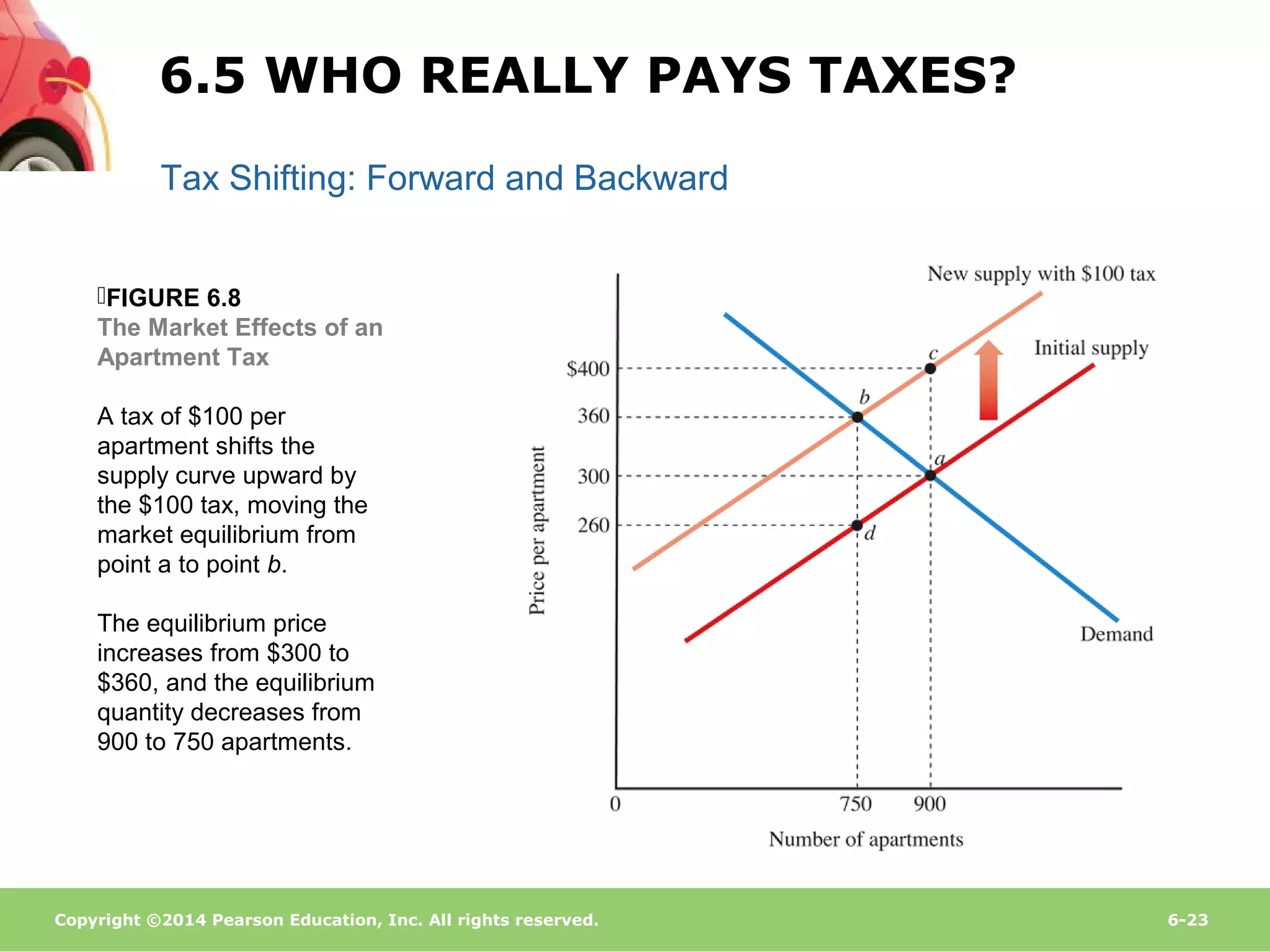
Tax Shifting: Forward and Backward
FIGURE 6.8
The Market Effects of an
Apartment Tax
A tax of $100 per
apartment shifts the
supply curve upward by
the $100 tax, moving the
market equilibrium from
point a to point b.
The equilibrium price
increases from $300 to
$360, and the equilibrium
quantity decreases from
900 to 750 apartments.
6.5 WHO REALLY PAYS TAXES?
Copyright ©2014 Pearson Education, Inc. All rights reserved. 6-24
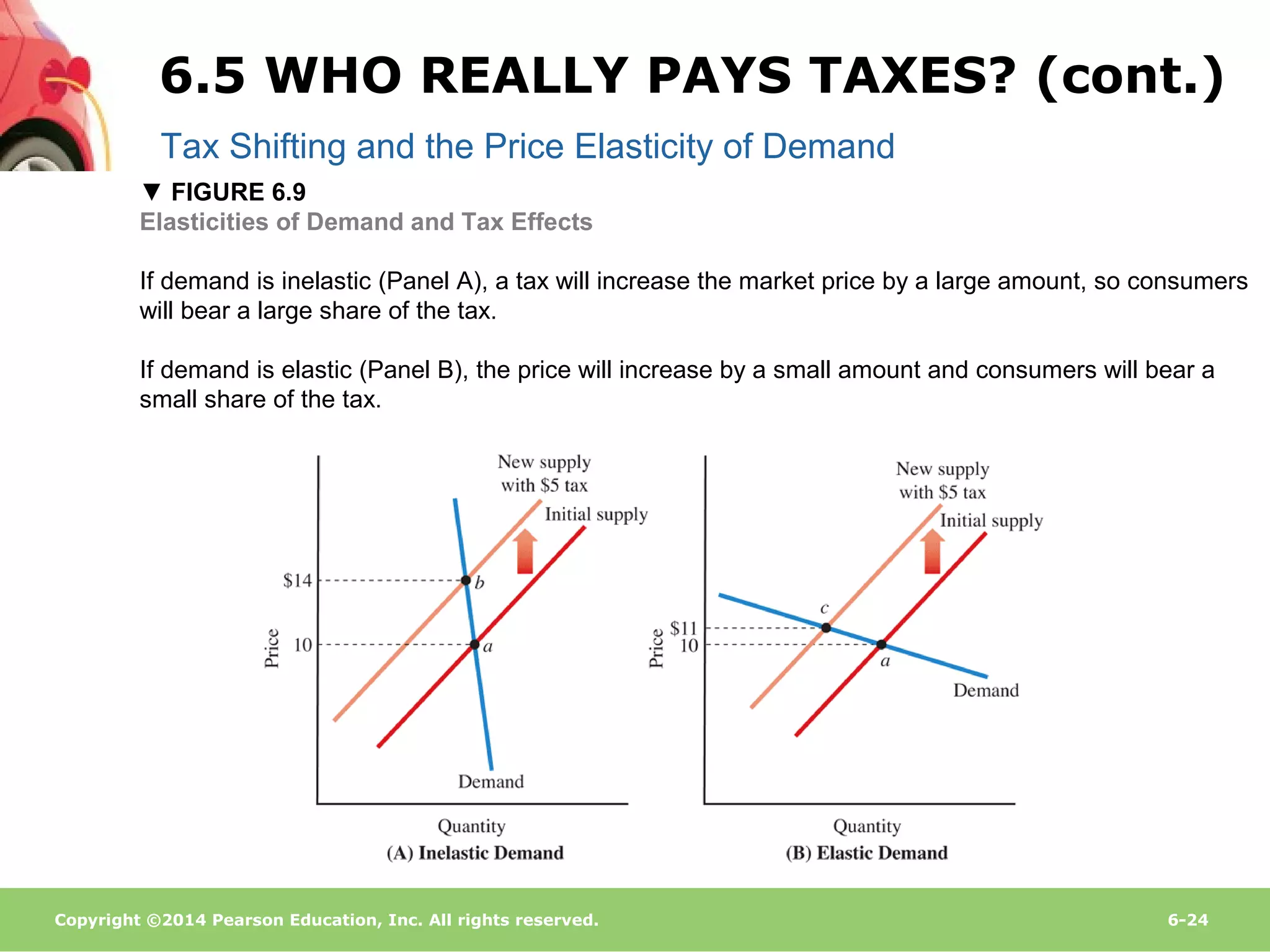
Tax Shifting and the Price Elasticity of Demand
▼ FIGURE 6.9
Elasticities of Demand and Tax Effects
If demand is inelastic (Panel A), a tax will increase the market price by a large amount, so consumers
will bear a large share of the tax.
If demand is elastic (Panel B), the price will increase by a small amount and consumers will bear a
small share of the tax.
6.5 WHO REALLY PAYS TAXES? (cont.)
Copyright ©2014 Pearson Education, Inc. All rights reserved. 6-25
Cigarette Taxes and Tobacco Land
• In 1994, President Clinton proposed an immediate $0.75 per pack increase in the
cigarette tax.
• The tax had two purposes:
▪ Generate revenue for Clinton’s health-care reform plan
▪ Decrease medical costs by discouraging smoking.
• Based on our discussion of the market effects of a tax, we would predict that the
tax would be shared by consumers, who would pay higher prices, and the owners
of land where tobacco is grown.
• It appears tobacco farmers and landowners understand the economics of cigarette
taxes. Led by a group of representatives and senators from tobacco-growing areas
in North Carolina, Kentucky, and Virginia, Congress scaled back Clinton’s proposed
tax hike from $0.75 to $0.05. Although the government would have collected the tax
from cigarette manufacturers, savvy tobacco farmers realized the tax would
decrease the price of their tobacco-growing land.
6.5 WHO REALLY PAYS TAXES? (cont.)
Copyright ©2014 Pearson Education, Inc. All rights reserved. 6-26
The Luxury Boat Tax and Boat Workers
• A lesson on backward shifting occurred when Congress passed a steep luxury tax
on boats and other luxury goods in 1990.
• Under the new tax, a person buying a $300,000 boat paid an additional $20,000 in
taxes.
• The burden of the tax was actually shared by consumers and input suppliers,
including people who worked in boat factories and boatyards.
• The tax increased the price of boats, and consumers bought fewer boats.
▪ The boat industry produced fewer boats.
▪ The resulting decrease in the demand for boat workers led to layoffs and
lower wages for those who managed to keep their jobs.
• Although the idea behind the luxury tax was to “soak the rich,” the tax actually
harmed low-income workers in the boat industry. The tax was repealed a few years
later.
6.5 WHO REALLY PAYS TAXES? (cont.)
Copyright ©2014 Pearson Education, Inc. All rights reserved. 6-27
Tax Burden and Deadweight Loss
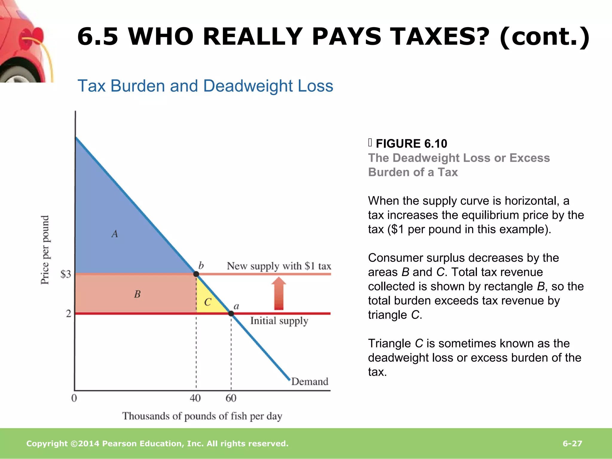
 FIGURE 6.10
The Deadweight Loss or Excess
Burden of a Tax
When the supply curve is horizontal, a
tax increases the equilibrium price by the
tax ($1 per pound in this example).
Consumer surplus decreases by the
areas B and C. Total tax revenue
collected is shown by rectangle B, so the
total burden exceeds tax revenue by
triangle C.
Triangle C is sometimes known as the
deadweight loss or excess burden of the
tax.
6.5 WHO REALLY PAYS TAXES? (cont.)
Copyright ©2014 Pearson Education, Inc. All rights reserved. 6-28
Tax Burden and Deadweight Loss
● deadweight loss from taxation
The difference between the total
burden of a tax and the amount of
revenue collected by the
government.
● excess burden of a tax
Another name for deadweight loss.
6.5 WHO REALLY PAYS TAXES? (cont.)
Copyright ©2014 Pearson Education, Inc. All rights reserved. 6-29
In France, regular restaurants pay a 20 percent value-added tax (VAT) on sit-down
meals, while fast-food restaurants pay just a 5 percent tax on take-away meals. A group
of large restaurant owners made the following pledge. If the nation were to cut its VAT
rate on restaurant meals to 5 percent, the owners would:
• cut the prices of restaurant meals by 5 percent;
• increase the wages paid to waiters and dishwashers by 10 percent.
The owners predicted that these changes would increase the quantity of restaurant meals
sold by 14 percent and increase restaurant employment by 40,000 workers.
Does the pledge of the restaurant owners make economic sense?
• Although the actual numbers in the owners’ pledge for lower prices and higher wages
may not be correct, the pledge is consistent with the economics of tax shifting.
RESPONSE TO LOWER TAXES IN
FRENCH RESTAURANTS
APPLYING THE CONCEPTS #5: How Does a Tax
Cut Affect Prices?
A P P L I C A T I O N 5
Copyright ©2014 Pearson Education, Inc. All rights reserved. 6-30
consumer surplus
deadweight loss
deadweight loss from taxation
efficiency
excess burden of a tax
price ceiling
price floor
producer surplus
total surplus
willingness to accept
willingness to pay
K E Y T E R M S

Econ 204 week 6 outline

  • 1.
    Prepared By BrockWilliams Chapter 6 Market Efficiency and Government Intervention The housing market in New York City is highly regulated. The city issues a relatively small number of permits for new condominium buildings, and rapid growth in the demand for condominiums has resulted in soaring condominium prices.
  • 2.
    Copyright ©2014 PearsonEducation, Inc. All rights reserved. 6-2 Learning Objectives 1. Use demand and supply curves to compute the value of markets 2. Explain why the market equilibrium maximizes the value of a market 3. Describe the market effects of price controls 4. Describe the market effects of quantity controls 5. Explain how a tax is shifted to consumers and input suppliers
  • 3.
    Copyright ©2014 PearsonEducation, Inc. All rights reserved. 6-3 ● efficiency A situation in which people do the best they can, given their limited resources. A market equilibrium will generate the largest possible surplus when four conditions are met: • No external benefits: The benefits of a product (a good or service) are confined to the person who pays for it. • No external costs: The cost of producing a product is confined to the person who sells it. • Perfect information: Buyers and sellers know enough about the product to make informed decisions about whether to buy or sell it. • Perfect competition: Each firm produces such a small quantity that the firm cannot affect the price. P R I N C I P L E O F V O L U N T A R Y E X C H A N G E A voluntary exchange between two people makes both people better off. Market Efficiency and Government Intervention
  • 4.
    Copyright ©2014 PearsonEducation, Inc. All rights reserved. 6-4 ● willingness to pay The maximum amount a consumer is willing to pay for a product. The Demand Curve and Consumer Surplus ● consumer surplus The amount a consumer is willing to pay for a product minus the price the consumer actually pays. 6.1 CONSUMER SURPLUS AND PRODUCER SURPLUS
  • 5.
    Copyright ©2014 PearsonEducation, Inc. All rights reserved. 6-5 The Demand Curve and Consumer Surplus ► FIGURE 6.1 The Demand Curve and Consumer Surplus Consumer surplus equals the maximum amount a consumer is willing to pay (shown by the demand curve) minus the price paid. Juan is willing to pay $22, so if the price is $10, his consumer surplus is $12. The market consumer surplus equals the sum of the surpluses earned by all consumers in the market. In this case, the market consumer surplus is $30 = $12 + $9 + $6 + $3 + $0. 6.1 CONSUMER SURPLUS AND PRODUCER SURPLUS (cont.)
  • 6.
    Copyright ©2014 PearsonEducation, Inc. All rights reserved. 6-6 The Supply Curve and Producer Surplus ● willingness to accept The minimum amount a producer is willing to accept as payment for a product; equal to the marginal cost of production. ● producer surplus The price a producer receives for a product minus the marginal cost of production. 6.1 CONSUMER SURPLUS AND PRODUCER SURPLUS (cont.)
  • 7.
    Copyright ©2014 PearsonEducation, Inc. All rights reserved. 6-7 The Supply Curve and Producer Surplus  FIGURE 6.2 The Supply Curve and Producer Surplus Producer surplus equals the market price minus the producer’s willingness to accept, or marginal cost (shown by the supply curve). Abe’s marginal cost is $2, so if the price is $10, his producer surplus is $8. The market producer surplus equals the sum of the surpluses earned by all producers in the market. In this case, the market producer surplus is $20 = $8 + $6 + $4 + $2 + $0. 6.1 CONSUMER SURPLUS AND PRODUCER SURPLUS (cont.)
  • 8.
    Copyright ©2014 PearsonEducation, Inc. All rights reserved. 6-8 • What is the consumer surplus from Internet service? Two recent studies compute consumers’ willingness to pay for Internet service. For Japanese consumers, the average willingness to pay for Internet service (email and web browsing delivered over personal computers) is $5,623 per month, compared to an average price of broadband Internet service of $4,000. • In other words, the average consumer surplus is $1,623, or about 40 percent of the price. • For US consumers, the average willingness to pay for Internet service is $85 per month, and with an average monthly price of $40, the consumer surplus is $45 per month. COMPUTER SURPLUS OF INTERNET SERICES APPLYING THE CONCEPTS #1: How do we compute consumer surplus? A P P L I C A T I O N 1
  • 9.
    Copyright ©2014 PearsonEducation, Inc. All rights reserved. 6-9  FIGURE 6.3 Market Equilibrium and the Total Market Surplus The total surplus of the market equals consumer surplus (the lightly shaded areas) plus producer surplus (the darkly shaded areas). The market equilibrium generates the highest possible total market value, equal to $50 = $30 (consumer surplus) + $20 (producer surplus). ● total surplus The sum of consumer surplus and producer surplus. 6.2 MARKET EQUILIBRIUM AND EFFICIENCY
  • 10.
    Copyright ©2014 PearsonEducation, Inc. All rights reserved. 6-10 Total Surplus Is Lower with a Price below the Equilibrium Price ● price ceiling A maximum price set by the government. Total Surplus Is Lower with a Price above the Equilibrium Price ● price floor A minimum price set by the government. 6.2 MARKET EQUILIBRIUM AND EFFICIENCY (cont.)
  • 11.
    Copyright ©2014 PearsonEducation, Inc. All rights reserved. 6-11 Total Surplus Is Lower with a Price above the Equilibrium Price  FIGURE 6.4 Price Controls Decrease the Total Surplus of the Market (A) A maximum price of $4 reduces the total surplus of the market. The first two consumers gain at the expense of the first two producers. The consumer and producer surpluses for the third and fourth lawns are lost entirely, so the total value of the market decreases. (B) A minimum price of $19 reduces the total surplus of the market. The first two producers gain at the expense of the first two consumers. The consumer and producer surpluses for the third and fourth lawns are lost entirely, so the total value of the market decreases. 6.2 MARKET EQUILIBRIUM AND EFFICIENCY (cont.)
  • 12.
    Copyright ©2014 PearsonEducation, Inc. All rights reserved. 6-12 Efficiency and the Invisible Hand The market equilibrium maximizes the total surplus of the market because it guarantees that all mutually beneficial transactions will happen. Instead of using a bureaucrat to coordinate the actions of everyone in the market, we can rely on the actions of individual consumers and individual producers, each guided only by self-interest. This is Adam Smith’s invisible hand in action. In most modern economies, governments take an active role. For a market that meets the four efficiency conditions, the market equilibrium generates the largest possible total surplus, so government intervention can only decrease the surplus and cause inefficiency. Government Intervention in Efficient Markets 6.2 MARKET EQUILIBRIUM AND EFFICIENCY (cont.)
  • 13.
    Copyright ©2014 PearsonEducation, Inc. All rights reserved. 6-13 • Under rent control, the government sets a maximum price for housing, decreasing the quantity supplied and the total value of the market. Rent control and other maximum prices cause inefficiency of another sort. • Consider a consumer living in a rent-controlled apartment who experiences a change in circumstances that would normally cause the consumer to a move to a different apartment. For example, when a single person renting a tiny apartment gets married, he or she is likely to move to a larger place. But a consumer in a rent- controlled apartment may stay in the tiny but inexpensive apartment, generating a housing mismatch. A recent study suggests that in New York City, about 20 percent of rent-controlled apartments are mismatched. • The most famous case of a mismatched tenant is former Mayor Koch of New York. When he was elected mayor and moved into the mayor’s official residence, he held onto his rent-controlled apartment, presumably anticipating his post-mayor life in an apartment at a controlled rent that was roughly one-third the market rent. RENT CONTROL AND MISMATCHES APPLYING THE CONCEPTS #2: Why does the market equilibrium maximize the value of a market? A P P L I C A T I O N 2
  • 14.
    Copyright ©2014 PearsonEducation, Inc. All rights reserved. 6-14 Setting Maximum Prices Here are some examples of goods that have been subject to maximum prices or may be subject to maximum prices in the near future: • Rental housing. • Gasoline. • Medical goods and services. In all three cases, a maximum price will cause excess demand and reduce the total surplus of the market. 6.3 CONTROLLING PRICES—MAXIMUM AND MINIMUM PRICES
  • 15.
    Copyright ©2014 PearsonEducation, Inc. All rights reserved. 6-15 Rent Control  FIGURE 6.5 Rent Control Decreases Total Surplus (A) In the market equilibrium, with a price of $400 and 1,000 apartments, the total surplus is the area between the demand curve and the supply curve. (B) Rent control, with a maximum price of $300, reduces the quantity to 700 apartments and decreases the total surplus.● deadweight loss The decrease in the total surplus of the market that results from a policy such as rent control. 6.3 CONTROLLING PRICES—MAXIMUM AND MINIMUM PRICES (cont.)
  • 16.
    Copyright ©2014 PearsonEducation, Inc. All rights reserved. 6-16 Rent Control Because rent control outlaws transactions that would make both parties better off, it causes inefficiency. Three more subtle effects associated with rent control add to its inefficiency: • Search costs. • Cheating. • Decrease in quality of housing. P R I N C I P L E O F V O L U N T A R Y E X C H A N G E A voluntary exchange between two people makes both people better off. 6.3 CONTROLLING PRICES—MAXIMUM AND MINIMUM PRICES (cont.)
  • 17.
    Copyright ©2014 PearsonEducation, Inc. All rights reserved. 6-17 Setting Minimum Prices • Recall that when government sets a minimum price above the equilibrium price, the result is permanent excess supply. • Governments around the world establish minimum prices for agricultural goods. • Under a price-support program, a government sets a minimum price for an agricultural product and then buys any resulting surpluses at that price. 6.3 CONTROLLING PRICES—MAXIMUM AND MINIMUM PRICES (cont.)
  • 18.
    Copyright ©2014 PearsonEducation, Inc. All rights reserved. 6-18 • During World War II, the U.S. government used a system of price controls to set maximum prices on all sorts of products, including candy bars. • Consumer Reports compared the weights of candy bars in 1943 to their weights in 1939, before the maximum prices were imposed. In 19 of 20 cases, the candy bars had shrunk, causing the price per ounce to increase by an average of 23 percent. • In other words, producers reacted to maximum prices by shrinking candy bars to match the relatively low maximum price. In the words of Consumer Reports, the shrinkage of candy bars is an example of “hidden price increases.” PRICE CONTROLS AND THE SHRINKING CANDY BAR APPLYING THE CONCEPTS #3: How Do Price Controls Affect the Market? A P P L I C A T I O N 3
  • 19.
    Copyright ©2014 PearsonEducation, Inc. All rights reserved. 6-19 Taxi Medallions ▼ FIGURE 6.6 The Market Effects of Taxi Medallions (A) The market equilibrium is shown by point a, with a price of $3.00 and a quantity of 10,000 miles of service per day (100 taxis and 100 miles per taxi). The total surplus is the area between the demand and supply curves. (B) A medallion policy reduces the quantity of taxi service to 8,000 miles per day (80 taxis and 100 miles per taxi) and increases the price to $3.60 (point c). The producers of the first 8,000 miles gain at the expense of consumers, but the surpluses for between 8,000 and 10,000 miles are lost entirely. Therefore, the total surplus decreases. 6.4 CONTROLLING QUANTITIES—LICENSING AND IMPORT RESTRICTIONS
  • 20.
    Copyright ©2014 PearsonEducation, Inc. All rights reserved. 6-20 Licensing and Market Efficiency Winners and Losers from Licensing Our analysis of taxi medallions applies to any market subject to quantity controls. In general, a policy that limits entry into a market ▪ increases price, ▪ decreases quantity, and ▪ causes inefficiency in the market. In evaluating such a policy, we must compare the possible benefits from controlling nuisances to the losses of consumer and producer surplus. Who benefits and who loses from licensing programs such as a taxi medallion policy? The losers are consumers, who pay more for taxi rides. The winners are the people who receive a free medallion and the right to charge an artificially high price for taxi service. 6.4 CONTROLLING QUANTITIES—LICENSING AND IMPORT RESTRICTIONS (cont.)
  • 21.
    Copyright ©2014 PearsonEducation, Inc. All rights reserved. 6-21 Import Restrictions ▼ FIGURE 6.7 The Effects of an Import Ban on U.S. Prices and Consumer and Producer Surplus (A) With free trade, the demand intersects the total supply curve at point a with a price of $0.12 and a quantity of 360 million pounds. This price is below the minimum price of domestic suppliers ($0.26, as shown by point m), so domestic firms do not participate in the market. The total surplus is shown by the shaded areas (U.S. consumer surplus and foreign producer surplus). (B) If sugar imports are banned, the equilibrium is shown by the intersection of the demand curve and the domestic (U.S.) supply curve (point b). The price increases to $0.30. Although the ban generates a producer surplus for domestic producers, their gain is less than the loss of domestic consumers. 6.4 CONTROLLING QUANTITIES—LICENSING AND IMPORT RESTRICTIONS (cont.)
  • 22.
    Copyright ©2014 PearsonEducation, Inc. All rights reserved. 6-22 • What is the cost of using import restrictions to protect jobs in the luggage industry? Luggage and handbags are subject to import quotas (quantity restrictions) and tariffs (import taxes) that decrease the supply of luggage and increase the price to consumers by 13 percent. • These policies protect about 226 jobs in the industry and reduce consumer surplus by $290 million, so the cost per job protected is roughly $1.29 million per year. • Similar calculations show that the cost per job protected is $826,000 for the sugar industry, $685,000 for the dairy industry, and $199,000 for the apparel industry. THE COST OF PROTECTING A LUGGAGE JOB APPLYING THE CONCEPTS #4: What Are The Effects of Import Restrictions? A P P L I C A T I O N 4
  • 23.
    Copyright ©2014 PearsonEducation, Inc. All rights reserved. 6-23 Tax Shifting: Forward and Backward FIGURE 6.8 The Market Effects of an Apartment Tax A tax of $100 per apartment shifts the supply curve upward by the $100 tax, moving the market equilibrium from point a to point b. The equilibrium price increases from $300 to $360, and the equilibrium quantity decreases from 900 to 750 apartments. 6.5 WHO REALLY PAYS TAXES?
  • 24.
    Copyright ©2014 PearsonEducation, Inc. All rights reserved. 6-24 Tax Shifting and the Price Elasticity of Demand ▼ FIGURE 6.9 Elasticities of Demand and Tax Effects If demand is inelastic (Panel A), a tax will increase the market price by a large amount, so consumers will bear a large share of the tax. If demand is elastic (Panel B), the price will increase by a small amount and consumers will bear a small share of the tax. 6.5 WHO REALLY PAYS TAXES? (cont.)
  • 25.
    Copyright ©2014 PearsonEducation, Inc. All rights reserved. 6-25 Cigarette Taxes and Tobacco Land • In 1994, President Clinton proposed an immediate $0.75 per pack increase in the cigarette tax. • The tax had two purposes: ▪ Generate revenue for Clinton’s health-care reform plan ▪ Decrease medical costs by discouraging smoking. • Based on our discussion of the market effects of a tax, we would predict that the tax would be shared by consumers, who would pay higher prices, and the owners of land where tobacco is grown. • It appears tobacco farmers and landowners understand the economics of cigarette taxes. Led by a group of representatives and senators from tobacco-growing areas in North Carolina, Kentucky, and Virginia, Congress scaled back Clinton’s proposed tax hike from $0.75 to $0.05. Although the government would have collected the tax from cigarette manufacturers, savvy tobacco farmers realized the tax would decrease the price of their tobacco-growing land. 6.5 WHO REALLY PAYS TAXES? (cont.)
  • 26.
    Copyright ©2014 PearsonEducation, Inc. All rights reserved. 6-26 The Luxury Boat Tax and Boat Workers • A lesson on backward shifting occurred when Congress passed a steep luxury tax on boats and other luxury goods in 1990. • Under the new tax, a person buying a $300,000 boat paid an additional $20,000 in taxes. • The burden of the tax was actually shared by consumers and input suppliers, including people who worked in boat factories and boatyards. • The tax increased the price of boats, and consumers bought fewer boats. ▪ The boat industry produced fewer boats. ▪ The resulting decrease in the demand for boat workers led to layoffs and lower wages for those who managed to keep their jobs. • Although the idea behind the luxury tax was to “soak the rich,” the tax actually harmed low-income workers in the boat industry. The tax was repealed a few years later. 6.5 WHO REALLY PAYS TAXES? (cont.)
  • 27.
    Copyright ©2014 PearsonEducation, Inc. All rights reserved. 6-27 Tax Burden and Deadweight Loss  FIGURE 6.10 The Deadweight Loss or Excess Burden of a Tax When the supply curve is horizontal, a tax increases the equilibrium price by the tax ($1 per pound in this example). Consumer surplus decreases by the areas B and C. Total tax revenue collected is shown by rectangle B, so the total burden exceeds tax revenue by triangle C. Triangle C is sometimes known as the deadweight loss or excess burden of the tax. 6.5 WHO REALLY PAYS TAXES? (cont.)
  • 28.
    Copyright ©2014 PearsonEducation, Inc. All rights reserved. 6-28 Tax Burden and Deadweight Loss ● deadweight loss from taxation The difference between the total burden of a tax and the amount of revenue collected by the government. ● excess burden of a tax Another name for deadweight loss. 6.5 WHO REALLY PAYS TAXES? (cont.)
  • 29.
    Copyright ©2014 PearsonEducation, Inc. All rights reserved. 6-29 In France, regular restaurants pay a 20 percent value-added tax (VAT) on sit-down meals, while fast-food restaurants pay just a 5 percent tax on take-away meals. A group of large restaurant owners made the following pledge. If the nation were to cut its VAT rate on restaurant meals to 5 percent, the owners would: • cut the prices of restaurant meals by 5 percent; • increase the wages paid to waiters and dishwashers by 10 percent. The owners predicted that these changes would increase the quantity of restaurant meals sold by 14 percent and increase restaurant employment by 40,000 workers. Does the pledge of the restaurant owners make economic sense? • Although the actual numbers in the owners’ pledge for lower prices and higher wages may not be correct, the pledge is consistent with the economics of tax shifting. RESPONSE TO LOWER TAXES IN FRENCH RESTAURANTS APPLYING THE CONCEPTS #5: How Does a Tax Cut Affect Prices? A P P L I C A T I O N 5
  • 30.
    Copyright ©2014 PearsonEducation, Inc. All rights reserved. 6-30 consumer surplus deadweight loss deadweight loss from taxation efficiency excess burden of a tax price ceiling price floor producer surplus total surplus willingness to accept willingness to pay K E Y T E R M S