Dynamical systems simulation in Python for science and engineering

Python language in science and engineering
for the simulations
Dynamical
Systems
Simulation in
Python
Python frameworks and packages
for physical and dynamic
simulations
Engineer Massimo Talia-17/02/2024

1
Summary
Python frameworks and packages for physical and dynamic simulations.................................................... 0
List of figures.....................................................................................................................................................2
Installing Python................................................................................................................................................3
Introduction to the Python packages for the simulation...............................................................................7
Simupy package................................................................................................................................................ 9
Control package...............................................................................................................................................14
Plotly and Dash................................................................................................................................................23

2
List of figures
Figure 1-Python interpreter...............................................................................................................................3
Figure 2-PIP version.......................................................................................................................................... 4
Figure 3-PIP upgrade command ...................................................................................................................... 4
Figure 4-PIP packages list..................................................................................................................................5
Figure 5-PIP commands help.............................................................................................................................5
Figure 6-PY command help.............................................................................................................................. 6
Figure 7-Python command help....................................................................................................................... 6
Figure 8-Python packaging user guide.............................................................................................................7
Figure 9-Python packaging index.....................................................................................................................7
Figure 10-Simupy package................................................................................................................................ 9
Figure 11- mass, spring, damper system .......................................................................................................... 9
Figure 12-Control scheme at closed loop PID.................................................................................................10
Figura 13-Closed loop PID response................................................................................................................ 13
Figure 14- Transfer function response............................................................................................................ 15
Figure 15-Bode diagram...................................................................................................................................16
Figure 16-LQR problem input data.................................................................................................................. 17
Figure 17-Aircraft trajectory control simulation.............................................................................................18
Figure 18-Plotly package..................................................................................................................................23
Figure 19-Dash package...................................................................................................................................23
Figure 20-Smith Chart by Plotly ......................................................................................................................24
Figure 21-Smith chart by Dash.........................................................................................................................25

3
Installing Python
Python is a high-level object-oriented interpreted language developed on February 1991 by Guido Van
Rossum suited for developing distributed applications, scripting, numerical computation and system
testing as well. Visit https://www.python.org/ and click on the download menu and choose Windows,
Linux or mac OS operating systems in order to download the Python interpreter.
Figure 1-Python interpreter
Once you have installed the interpreter according to the instructions from the website above and have
set the environment variable on Windows during installation, proceed with the installation of the
simulation frameworks or plugins by the package installer for Python named PIP. For further
information about PIP, visit https://pip.pypa.io/en/stable/. Then type Windows logo button + R and
write CMD command in the DOS prompt of Windows. When the DOS prompt of Windows is open, check
the PIP version by the command of the image below.

4
Figure 2-PIP version
If the PIP version is not updated to the latest version, type the command shown in the following figure
in the DOS prompt, restarting the DOS prompt as an administrator. As shown below, the PIP version is
the last one. In other cases PIP must be updated.
Figure 3-PIP upgrade command
Check you have not already installed the framework or package you need, scrolling through the list of
installed plugins using the command C:>py –m pip list in the DOS prompt or eventually DOS PowerShell
(if you’re using Windows, in other cases Linux or MacOS ,use the Shell of each one).

5
Figure 4-PIP packages list
For further information about PIP commands type C:>py –m pip, as you can see below.
Figure 5-PIP commands help

6
For information about the python commands type C:>py –h where you can choose the launcher
python interpreter version as well.
Figure 6-PY command help
If you want to know more about only the prompt python commands digit C:>python –h and you’ll
visualize the follow list in figure below.
Figure 7-Python command help

7
Introduction to the Python packages for the simulation
There are several packages for the scientific and engineering simulations in Python, it’s enough you
check the list of the available packages in the Python Packaging user guide by the web link
https://packaging.python.org/en/latest/overview/
Figure 8-Python packaging user guide
The list of the available packages are in the website https://pypi.org/ of Python packages index
Figure 9-Python packaging index

8
In this cases the choosed package for simulations are:
1. simupy
2. control
3. plotly and dash
For installing the package above its enough you digit C:>py –m pip install “name of the package”
where “name of the package” is the string name of the package. The name is available in the list of
Python package index. In the case of the package above the commands of installation are:
C:>py –m pip install simupy
C:>py –m pip install control
C:>py –m pip install plotly
C:>py –m pip install dash
If you have set the python interpreter link in the environment variable of Windows you can simply use
the commands:
C:>pip install simupy
C:>pip install control
C:>pip install plotly
C:>pip install dash
If you want upgrade the installation during the package download, then write:
C:>pip install –-upgrade simupy
C:>pip install –-upgrade control
C:>pip install –-upgrade plotly
C:>pip install –-upgrade dash
In the next pages will be described some cases in using the packages above.

9
Simupy package
From https://pypi.org/project/simupy/ you can know the last version of Simupy by Benjamin Margolis.
You can download example in Python.
Figure 10-Simupy package
The example below describes the use of Simupy in the PID calibration of a mass, spring, damper system
by the Zigler-Nichol methodology.
Figure 11- mass, spring, damper system
A mass, spring, damper system is an example that represents a simplified model of an oscillator, which
in the concrete world can be represented by the shock absorbers of a motor vehicle. The dynamic
variables or states are represented by the displacement s(t) and the derivative of the displacement or
velocity v(t)=(x(t)) . So in an ISO LTI representation, the state vector is:
X(t)=
The input u(t)= F(t) is the force to make the body oscillate, while the output is equal to the
displacement y(t)=s(t). In an open cycle the system oscillates dependently on the forcing and
uncontrollably, without being able to make it evolve in a desired manner.

10
The purpose of a closed-loop control filter is to stabilize oscillations and dynamic and static
performance according to specifications. In the case of the above system, the controller is the human
hand that varies the oscillations of the body. In general in the engineering applied to the real world, a
control system is a mechanism for controlling the performance of a product according to legal limits or
product requirements pre-established by the manufacturer. It can be of the following types:
electromechanical, mechanical, electrical, electronic, IT (industrial computers or PLCs). A matrix ISO
(Input State Output) representation of the system described previously is the following:
0 1
/ /
0
1/ 1 0 0
Where Ac and Bc are the dynamic matrices of the states C and D are related to the output. The system is
strictly proper since D=0.
PID control scheme at closed loop:
Figure 12-Control scheme at closed loop PID
The Ziegler-Nichols method for the calibration of PID (Proportional, Integral, Derivative) controllers,
dating back to 1942, is among the most used in industry and is appreciated for its simplicity, for the fact
that it does not require a mathematical model of the process and for the performances it manages to
produce. This is an algorithm to find the so-called "critical gain" Kc, from which the other PID
parameters will be derived.
Algorithm:
1. The process is controlled by an exclusively proportional controller (KI and KD are set to zero);
2. The gain K of the proportional controller is gradually increased;
3. The critical gain Ku is the value of the gain for which the controlled variable presents sustained
oscillations, i.e. which do not disappear after a transient: this is a measure of the effect of the delays
and the dynamics of the process;
4. The critical period Pu of the sustained oscillations is recorded.

11
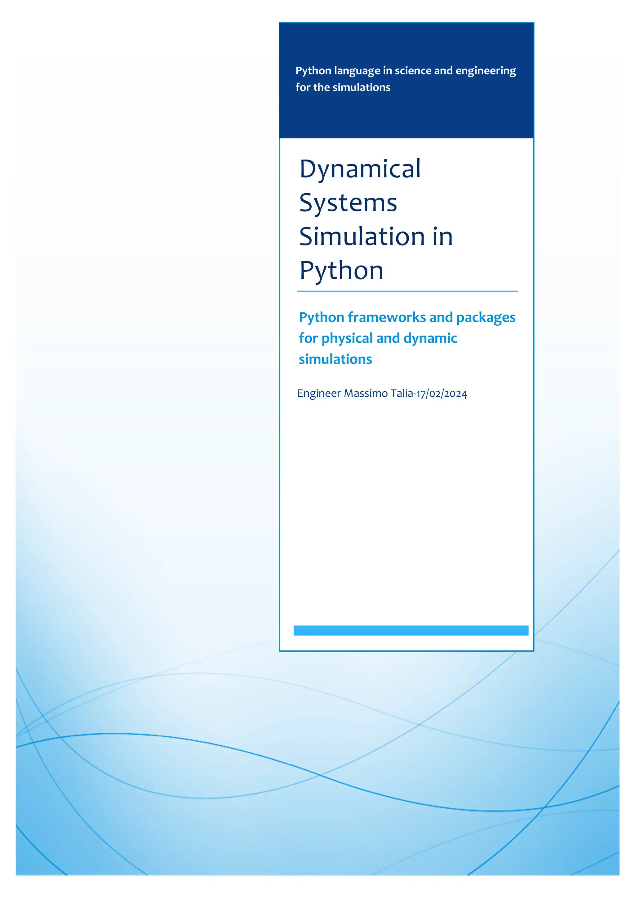
According to the following table, the constants for the P, PI or PID controller are determined:
Ziegler–Nichols calibration
Tipo Kp tau_I Tau_D
P 0,50Ku - -
PI 0,45Ku Pu/1,2 -
PID 0,60Ku Pu/2 Pu/8
Tabella 1-Ziegler-Nichols calibration
Algorithm PID in Python Simupy for calibrating the system and dynamical response:
import numpy as np
from scipy import signal, linalg
from simupy.systems import LTISystem, SystemFromCallable
from simupy.block_diagram import BlockDiagram
import matplotlib.pyplot as plt
from pylab import *
from scipy import signal
#Example implemented by Massimo Talia
#construct second order system state 2x2 (Mass-Spring-Damper) and input matrices
#Mass
m = 1
#External force u=d/m
d = 1
#Viscosity coefficient, damping ratio zita=b/2mxWn
b = 1
#Spring elongation coefficient, squared natural frequency Wn^2=k/m
k = 1
#s(t) displacement , v(t) speed
#Dynamical Matrices x=[s(t), v(t)], d(x)/d(t)=v(t), y(t)=s(t)=[1 0]*s(t)
#dim(Ac)=2x2, dim(Bc)=2x1, Dim(Cc)=1x2, dim(Dc)=0
Ac = np.c_[[0, -k/m], [1, -b/m]]
Bc = np.r_[0, d/m].reshape(-1, 1)
Cc= np.r_[1,0]
Dc=np.zeros((1,1))
#augment state and input matrices to add integral error state
A_aug = np.hstack((np.zeros((3,1)), np.vstack((np.r_[1, 0], Ac))))
B_aug = np.hstack(( np.vstack((0, Bc)), -np.eye(3,1)))
#construct the system LTI from augmented state matrices
aug_sys = LTISystem(A_aug, B_aug,)
#construct PID system by Ziegler-Nichols Method
#proportional coefficient
Kc = 1
#integral time constant tau_I
tau_I = 1
#derivative time constant tau_D
tau_D = 1
#Feedback Gain Matrix (1x3)
#K(s)=Kc*[(tau_I*s+1)/tau_I*s]*[(tau_D*s+1)/(alpha*tau_D*s+1)]

12
#alpha=0,05:0,2
#integral coefficient Ki=Kc/tau_I
#derivative coefficient Kd=Kc*tau_D
K = -np.r_[Kc/tau_I, Kc, Kc*tau_D].reshape((1,3))
#LTI system Gain Matrix
pid = LTISystem(K)
#construct reference (step u(t)=1(t))
ref = SystemFromCallable(lambda *args: np.ones(1), 0, 1)
#create block diagram
BD = BlockDiagram(aug_sys, pid, ref)
BD.connect(aug_sys, pid)
# PID requires feedback
BD.connect(pid, aug_sys, inputs=[0])
# PID output to system control input
BD.connect(ref, aug_sys, inputs=[1])
# reference output to system command input 20 seconds
res = BD.simulate(20)
#simulate
#plot
plt.figure('PID closed loop response')
plt.plot(res.t, res.y[:, 0], label=r'$int x(t)$')
plt.plot(res.t, res.y[:, 1], label='$y(t)=x(t)=s(t)$')
plt.plot(res.t, res.y[:, 2], label=r'$dot{x(t)}=v(t)$')
plt.plot(res.t, res.y[:, 3], label='$u(t)=Kp(t)+Ki(t)+Kd(t)$')
plt.plot(res.t, res.y[:, 4], label='ref=1*t')
plt.xlabel('seconds')
plt.ylabel('Closed loop outputs')
#Plot Grid
plt.grid(True, 'both', 'both')
plt.legend()
plt.show()
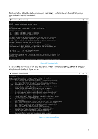
The closed-loop dynamic response was plotted with matplotlib.pyplot , which is in the packages
installed in the Python interpreter and needed in SimuPy to plot the graphs. In the legend there is a
description of the signals, in particular the three intermediate signals coming out of the PID control
block are traced, the closed loop signal u(t), the states x(t) and the controlled output y(t) with respect
to a ref reference of constant unit signal or unit step.

13
The constant input signal could be a DC signal or a constant input voltage.
Figura 13-Closed loop PID response

14
Control package
The control package control is located in https://pypi.org/project/control/ and it’s a Python package
which implements basic operations for analysis and design of feedback control systems.
The features of this package are:
1. Linear input/output systems in state-space and frequency domain
2. Block diagram algebra: serial, parallel, feedback, and other interconnections
3. Time response: initial, step, impulse
4. Frequency response: Bode, Nyquist, and Nichols plots
5. Control analysis: stability, reachability, observability, stability margins, root locus
6. Control design: eigenvalue placement, linear quadratic regulator, sisotool, hinfsyn,
rootlocus_pid_designer
7. Estimator design: linear quadratic estimator (Kalman filter)
8. Nonlinear systems: optimization-based control, describing functions, differential flatness
In the next pages we show the example code of frequency response and the Bode,, very used in
electronics for designing analogue and digital filters, the Linear Quadratic estimator problem o Kalman
filter problem.
Case 1:
Tracing the Bode diagram of the transfer function :
1
2 1

15
import numpy as np
from scipy import signal, linalg
import matplotlib.pyplot as plt
import control as cl
from control.matlab import*
from pylab import *
from scipy import signal
#Example implemented by Massimo Talia
#Bode Diagrams of Magnitude and Phase W(s)
plt.figure('Bode Diagrams')
num=np.array([1])
den1=np.array([1,1])
den2=np.array([1,1])
den=np.convolve(den1,den2)
W = cl.tf(num, den)
print ('W(s) =', W)
sys=cl.tf2ss(num,den)
w = np.logspace(-3,4)
mag,phase,omega = cl.bode(sys,w)
wc = np.interp(-180.0,np.flipud(phase),np.flipud(omega))
Kcu = np.interp(wc,omega,mag)
print('Crossover freq = ', wc, ' rad/sec')
print('Gain at crossover = ', Kcu)
plt.tight_layout()
plt.show()
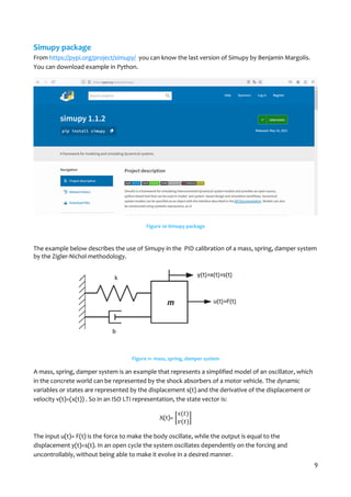
Figure 14- Transfer function response

17
Case 2:
LQR control design for vertical take-off and landing aircraft
This script demonstrates the use of the python-control package for analysis and design of a controller
for a vectored thrust aircraft model that is used as a running example through the text Feedback
Systems by Astrom and Murray. This example makes use of MATLAB compatible commands. Visit the
web link: https://python-control.readthedocs.io/en/0.9.4/pvtol-lqr.html
Data in input and state space representation is in the figure below.
Figure 16-LQR problem input data

18
Here the result of the simulation of take-off and landing aircraft trajectory control by LQR or Kalman
filter.
Figure 17-Aircraft trajectory control simulation
Visit the website https://python-control.readthedocs.io/en/0.9.4/examples.html in order to test and
verify some examples of the Python control package. Below you can find the source code to simulate:
import os
import numpy as np
import matplotlib.pyplot as plt # MATLAB plotting functions
from control.matlab import * # MATLAB-like functions
# System dynamics
# Implemented by Astrom and Murray
# These are the dynamics for the PVTOL system, written in state space
# form.
# System parameters
m = 4 # mass of aircraft
J = 0.0475 # inertia around pitch axis
r = 0.25 # distance to center of force
g = 9.8 # gravitational constant
c = 0.05 # damping factor (estimated)

19
# State space dynamics
xe = [0, 0, 0, 0, 0, 0] # equilibrium point of interest
ue = [0, m*g] # (note these are lists, not matrices)
# TODO: The following objects need converting from np.matrix to np.array
# This will involve re-working the subsequent equations as the shapes
# See below.
# Dynamics matrix (use matrix type so that * works for multiplication)
A = np.matrix(
[[0, 0, 0, 1, 0, 0],
[0, 0, 0, 0, 1, 0],
[0, 0, 0, 0, 0, 1],
[0, 0, (-ue[0]*np.sin(xe[2]) - ue[1]*np.cos(xe[2]))/m, -c/m, 0, 0],
[0, 0, (ue[0]*np.cos(xe[2]) - ue[1]*np.sin(xe[2]))/m, 0, -c/m, 0],
[0, 0, 0, 0, 0, 0]]
)
# Input matrix
B = np.matrix(
[[0, 0], [0, 0], [0, 0],
[np.cos(xe[2])/m, -np.sin(xe[2])/m],
[np.sin(xe[2])/m, np.cos(xe[2])/m],
[r/J, 0]]
)
# Output matrix
C = np.matrix([[1, 0, 0, 0, 0, 0], [0, 1, 0, 0, 0, 0]])
D = np.matrix([[0, 0], [0, 0]])
#
# Construct inputs and outputs corresponding to steps in xy position
#
# The vectors xd and yd correspond to the states that are the desired
# equilibrium states for the system. The matrices Cx and Cy are the
# corresponding outputs.
#
# The way these vectors are used is to compute the closed loop system
# dynamics as
#
# xdot = Ax + B u => xdot = (A-BK)x + K xd
# u = -K(x - xd) y = Cx
#
# The closed loop dynamics can be simulated using the "step" command,
# with K*xd as the input vector (assumes that the "input" is unit size,
# so that xd corresponds to the desired steady state.
#
xd = np.matrix([[1], [0], [0], [0], [0], [0]])
yd = np.matrix([[0], [1], [0], [0], [0], [0]])
#
# Extract the relevant dynamics for use with SISO library

20
#
# The current python-control library only supports SISO transfer
# functions, so we have to modify some parts of the original MATLAB
# code to extract out SISO systems. To do this, we define the 'lat' and
# 'alt' index vectors to consist of the states that are are relevant
# to the lateral (x) and vertical (y) dynamics.
#
# Indices for the parts of the state that we want
lat = (0, 2, 3, 5)
alt = (1, 4)
# Decoupled dynamics
Ax = (A[lat, :])[:, lat] # ! not sure why I have to do it this way
Bx = B[lat, 0]
Cx = C[0, lat]
Dx = D[0, 0]
Ay = (A[alt, :])[:, alt] # ! not sure why I have to do it this way
By = B[alt, 1]
Cy = C[1, alt]
Dy = D[1, 1]
# Label the plot
plt.clf()
plt.suptitle("LQR controllers for vectored thrust aircraft (pvtol-lqr)")
#
# LQR design
#
# Start with a diagonal weighting
Qx1 = np.diag([1, 1, 1, 1, 1, 1])
Qu1a = np.diag([1, 1])
K, X, E = lqr(A, B, Qx1, Qu1a)
K1a = np.matrix(K)
# Close the loop: xdot = Ax - B K (x-xd)
# Note: python-control requires we do this 1 input at a time
# H1a = ss(A-B*K1a, B*K1a*concatenate((xd, yd), axis=1), C, D);
# (T, Y) = step(H1a, T=np.linspace(0,10,100));
# TODO: The following equations will need modifying when converting from np.matrix to np.array
# because the results and even intermediate calculations will be different with numpy arrays
# For example:
# Bx = B[lat, 0]
# Will need to be changed to:
# Bx = B[lat, 0].reshape(-1, 1)
# (if we want it to have the same shape as before)
# For reference, here is a list of the correct shapes of these objects:
# A: (6, 6)
# B: (6, 2)

21
# C: (2, 6)
# D: (2, 2)
# xd: (6, 1)
# yd: (6, 1)
# Ax: (4, 4)
# Bx: (4, 1)
# Cx: (1, 4)
# Dx: ()
# Ay: (2, 2)
# By: (2, 1)
# Cy: (1, 2)
# Step response for the first input
H1ax = ss(Ax - Bx*K1a[0, lat], Bx*K1a[0, lat]*xd[lat, :], Cx, Dx)
Yx, Tx = step(H1ax, T=np.linspace(0, 10, 100))
# Step response for the second input
H1ay = ss(Ay - By*K1a[1, alt], By*K1a[1, alt]*yd[alt, :], Cy, Dy)
Yy, Ty = step(H1ay, T=np.linspace(0, 10, 100))
plt.subplot(221)
plt.title("Identity weights")
# plt.plot(T, Y[:,1, 1], '-', T, Y[:,2, 2], '--')
plt.plot(Tx.T, Yx.T, '-', Ty.T, Yy.T, '--')
plt.plot([0, 10], [1, 1], 'k-')
plt.axis([0, 10, -0.1, 1.4])
plt.ylabel('position')
#Plot Grid added by Massimo Talia
plt.legend(('x', 'y'), loc='lower right')
# Look at different input weightings
Qu1a = np.diag([1, 1])
K1a, X, E = lqr(A, B, Qx1, Qu1a)
H1ax = ss(Ax - Bx*K1a[0, lat], Bx*K1a[0, lat]*xd[lat, :], Cx, Dx)
Qu1b = (40 ** 2)*np.diag([1, 1])
K1b, X, E = lqr(A, B, Qx1, Qu1b)
H1bx = ss(Ax - Bx*K1b[0, lat], Bx*K1b[0, lat]*xd[lat, :], Cx, Dx)
Qu1c = (200 ** 2)*np.diag([1, 1])
K1c, X, E = lqr(A, B, Qx1, Qu1c)
H1cx = ss(Ax - Bx*K1c[0, lat], Bx*K1c[0, lat]*xd[lat, :], Cx, Dx)
[Y1, T1] = step(H1ax, T=np.linspace(0, 10, 100))
[Y2, T2] = step(H1bx, T=np.linspace(0, 10, 100))
[Y3, T3] = step(H1cx, T=np.linspace(0, 10, 100))
plt.subplot(222)
plt.title("Effect of input weights")
plt.plot(T1.T, Y1.T, 'b-')
plt.plot([0, 10], [1, 1], 'k-')
plt.axis([0, 10, -0.1, 1.4])

22
# arcarrow([1.3, 0.8], [5, 0.45], -6)
plt.text(5.3, 0.4, 'rho')
# Output weighting - change Qx to use outputs
Qx2 = C.T*C
Qu2 = 0.1*np.diag([1, 1])
K, X, E = lqr(A, B, Qx2, Qu2)
K2 = np.matrix(K)
H2x = ss(Ax - Bx*K2[0, lat], Bx*K2[0, lat]*xd[lat, :], Cx, Dx)
H2y = ss(Ay - By*K2[1, alt], By*K2[1, alt]*yd[alt, :], Cy, Dy)
plt.subplot(223)
plt.title("Output weighting")
[Y2x, T2x] = step(H2x, T=np.linspace(0, 10, 100))
[Y2y, T2y] = step(H2y, T=np.linspace(0, 10, 100))
plt.plot(T2x.T, Y2x.T, T2y.T, Y2y.T)
plt.xlabel('time')
#
# Physically motivated weighting
#
# Shoot for 1 cm error in x, 10 cm error in y. Try to keep the angle
# less than 5 degrees in making the adjustments. Penalize side forces
# due to loss in efficiency.
#
Qx3 = np.diag([100, 10, 2*np.pi/5, 0, 0, 0])
Qu3 = 0.1*np.diag([1, 10])
(K, X, E) = lqr(A, B, Qx3, Qu3)
K3 = np.matrix(K)
H3x = ss(Ax - Bx*K3[0, lat], Bx*K3[0, lat]*xd[lat, :], Cx, Dx)
H3y = ss(Ay - By*K3[1, alt], By*K3[1, alt]*yd[alt, :], Cy, Dy)
plt.subplot(224)
# step(H3x, H3y, 10)
[Y3x, T3x] = step(H3x, T=np.linspace(0, 10, 100))
[Y3y, T3y] = step(H3y, T=np.linspace(0, 10, 100))
plt.plot(T3x.T, Y3x.T, T3y.T, Y3y.T)
plt.title("Physically motivated weights")
plt.xlabel('time')
if 'PYCONTROL_TEST_EXAMPLES' not in os.environ:
plt.show()

23
Plotly and Dash
From the Python package index you can find easy both Plotly and Dash. The links are:
https://pypi.org/project/plotly/ and https://pypi.org/project/dash/ . They are package for tracing
advanced graph for engineering and science.
Figure 18-Plotly package
Built on top of Plotly.js, React and Flask, Dash ties modern UI elements like dropdowns, sliders, and
graphs directly to your analytical Python code.
Figure 19-Dash package

24
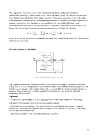
Case 1:
Trace the Smith chart (see https://www.antenna-theory.com/tutorial/smith/chart.php) of the impedance
3 2 by Plotly and Python
Figure 20-Smith Chart by Plotly
The source code of the Smith Chart is below and it’s based on Plotly tool of Python.
##Plotly for drawing the Smith Chart of an impedance, implemented by Massimo Talia
#Zn=3+2j
###############################################
import plotly.graph_objects as go
fig = go.Figure(go.Scattersmith(
real=[3],
imag=[2]
))
fig.update_traces(showlegend=True, legendgroup="group1", name="Z normal",
legendgrouptitle_text="Impedance Zn",marker_symbol='x',marker_size=10, marker=dict(angle=45,
angleref="up"), text="Zn", selector=dict(type='scattersmith'))
fig.show()

25
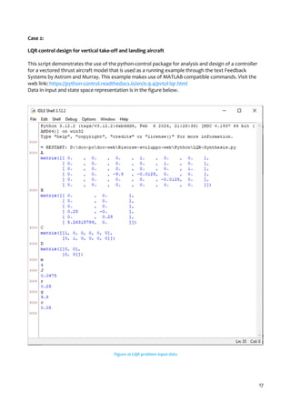
Case 2:
Trace the Smith chart (see https://www.antenna-theory.com/tutorial/smith/chart.php) of the
impedances 1 and 3 2 by Dash and Python.
Figure 21-Smith chart by Dash
The source code of the simulation is:
import dash
#import dash_core_components as dcc (old version)
from dash import dcc
#import dash_html_components as html (old version)
from dash import html
#Implemented by Massimo Talia
#Two impedances Zn1=1+jw and Zn2=3+2jw
fig.add_trace(go.Scattersmith(
imag=[1],
real=[1],
marker_symbol='x',
marker_size=30,
marker_color="green",
subplot="smith1"
))
fig.add_trace(go.Scattersmith(
imag=[3],
real=[2],
marker_symbol='x',
marker_size=30,
marker_color="pink",
subplot="smith2"
))

26
fig.update_layout(
smith1=dict(
realaxis_gridcolor='red',
imaginaryaxis_gridcolor='blue',
domain=dict(x=[0,0.45])
),
smith2=dict(
realaxis_gridcolor='blue',
imaginaryaxis_gridcolor='red',
domain=dict(x=[0.55,1])
)
)
fig.update_smiths(bgcolor="lightgrey")
fig.show()
app = dash.Dash()
app.layout = html.Div([
dcc.Graph(figure=fig)
])
app.run_server(debug=True, use_reloader=False)
#Turn off reloader if inside Jupyter

Dynamical systems simulation in Python for science and engineering

Recommended

Recommended

More Related Content

Similar to Dynamical systems simulation in Python for science and engineering

Similar to Dynamical systems simulation in Python for science and engineering (20)

More from Massimo Talia

More from Massimo Talia (20)

Recently uploaded

Recently uploaded (20)

Dynamical systems simulation in Python for science and engineering