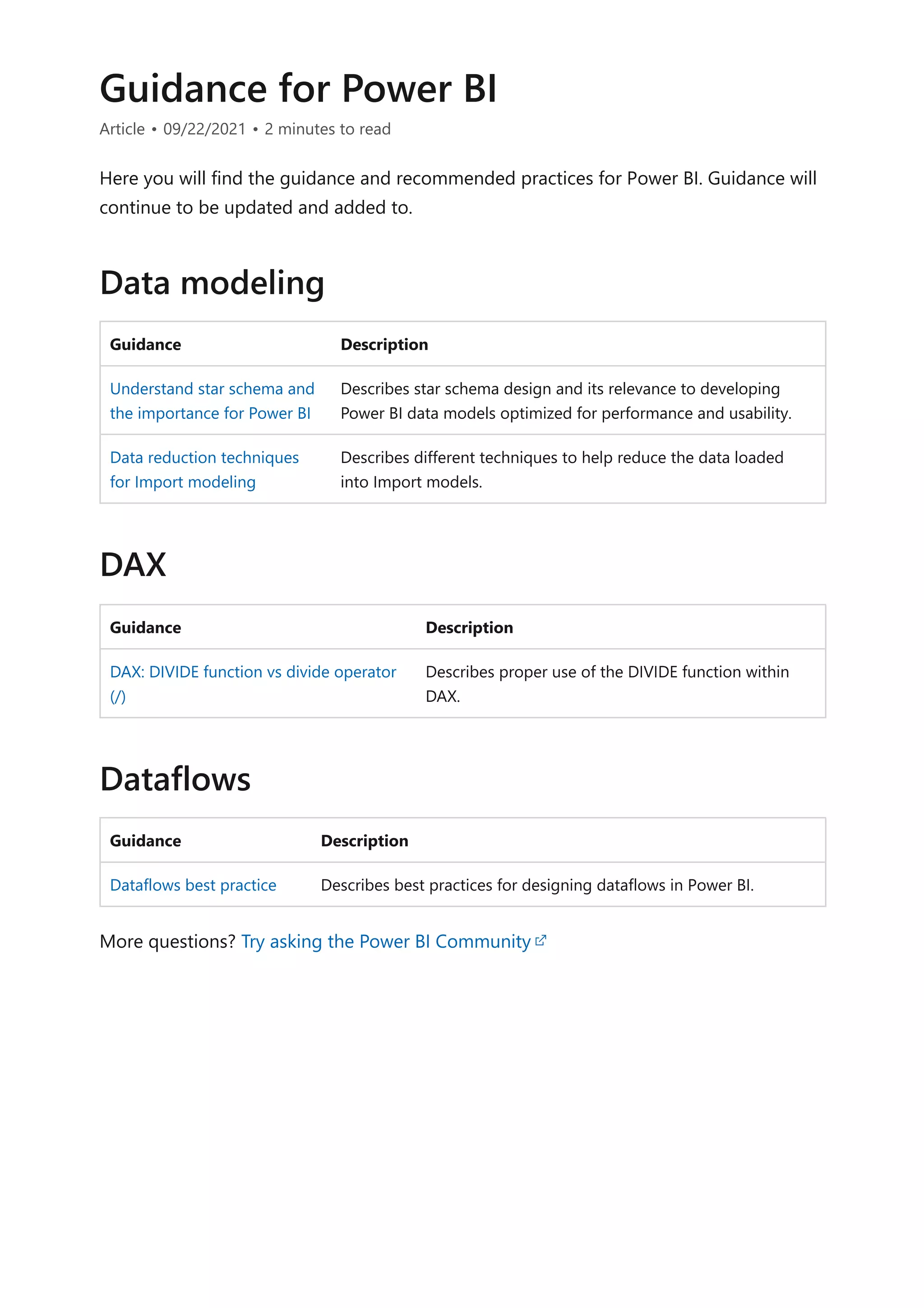
The document provides comprehensive Power BI guidance, including best practices for optimizing data modeling, visualizations, and report performance. It covers various topics such as query folding, DAX usage, report design, and managing capacity settings to improve overall efficiency. Updates and new information will continue to be added to assist users in maximizing the potential of Power BI solutions.


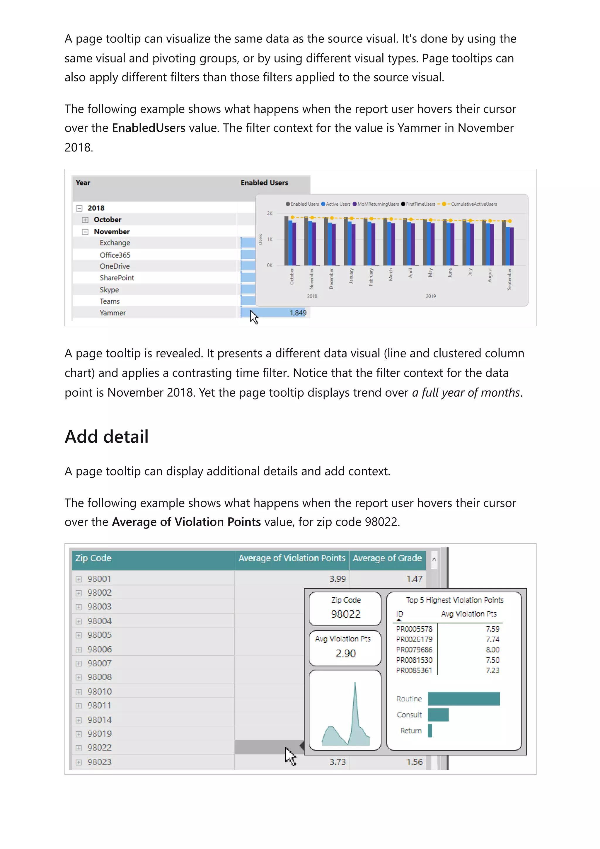
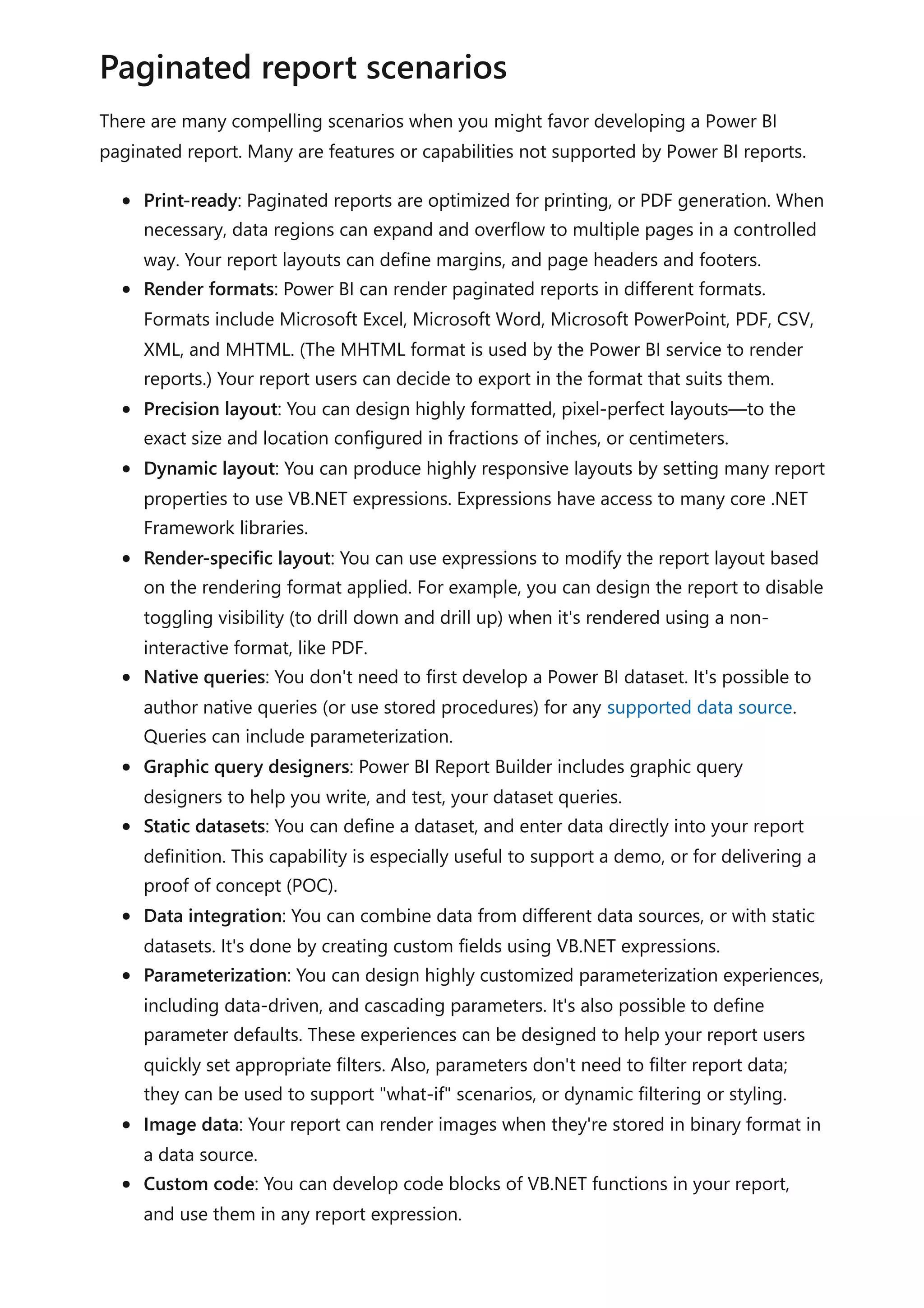
![column table of dates. You can then extend the calculated table with calculated columns
to support your date interval filtering and grouping requirements.
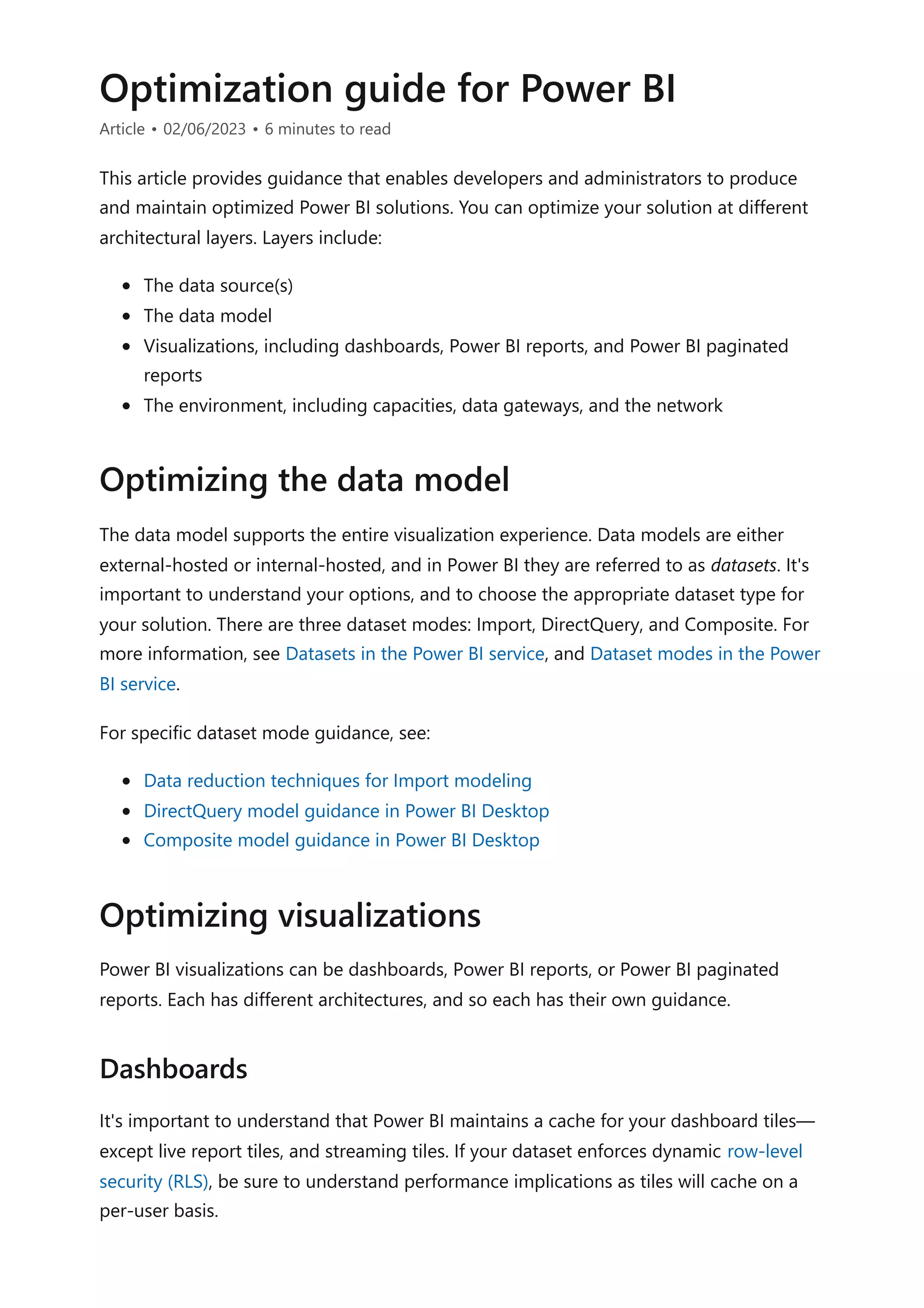
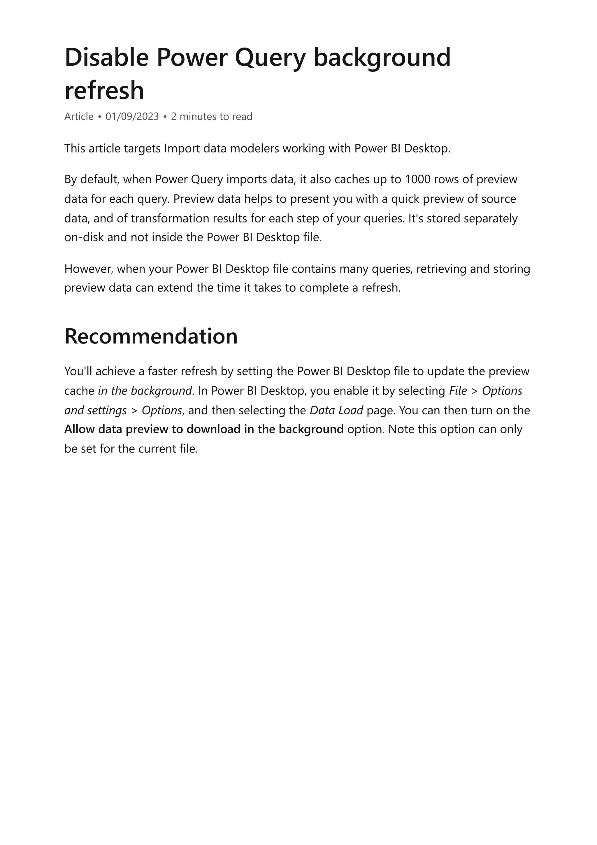
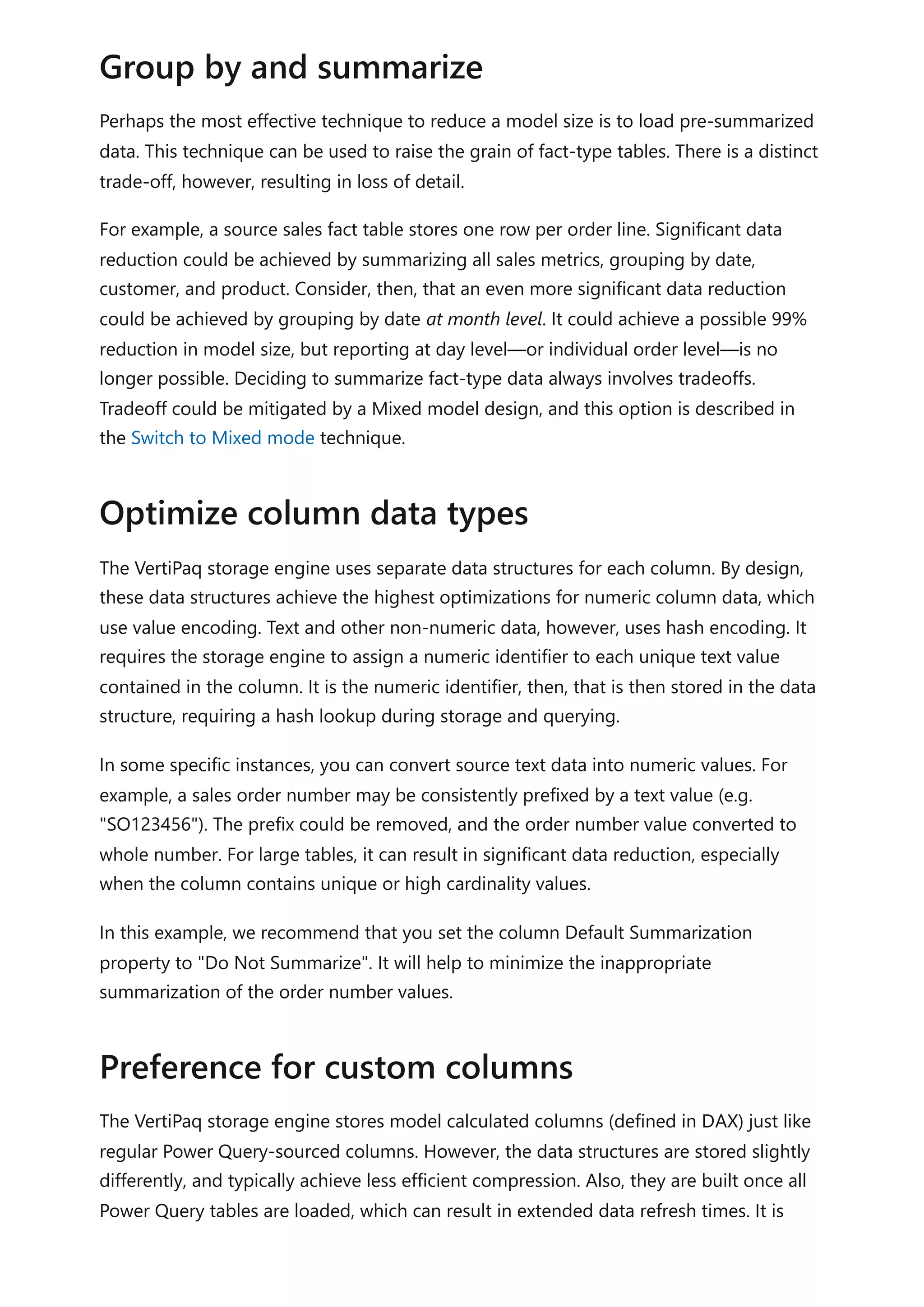
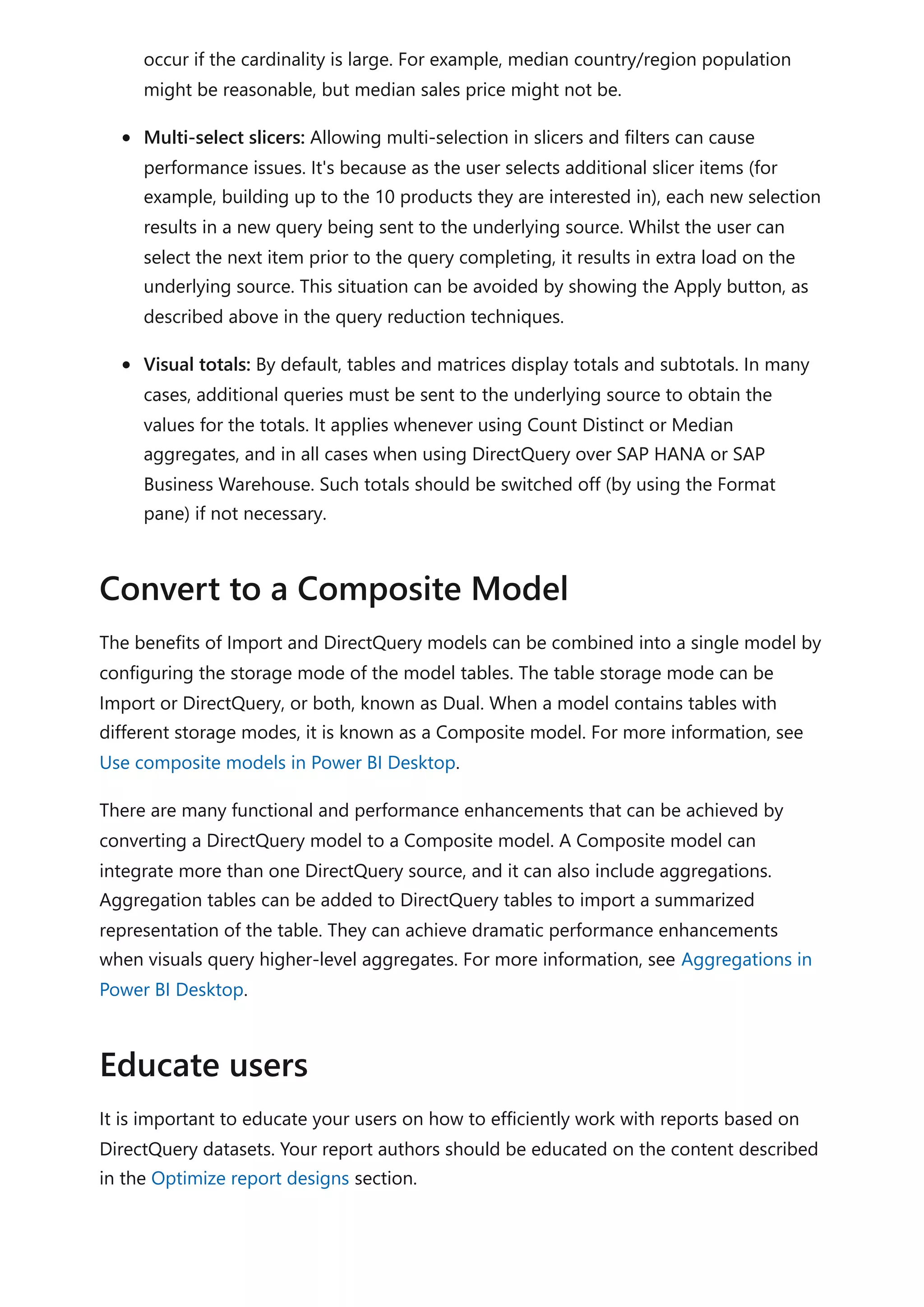
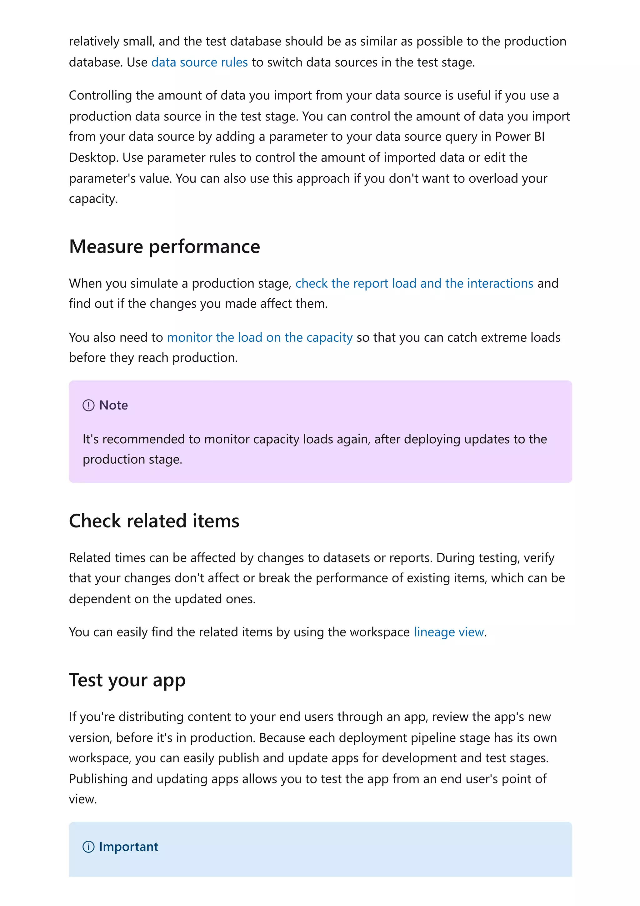
Use the CALENDAR function when you want to define a date range. You pass in
two values: the start date and end date. These values can be defined by other DAX
functions, like MIN(Sales[OrderDate]) or MAX(Sales[OrderDate]).
Use the CALENDARAUTO function when you want the date range to automatically
encompass all dates stored in the model. You can pass in a single optional
parameter that's the end month of the year (if your year is a calendar year, which
ends in December, you don't need to pass in a value). It's a helpful function,
because it ensures that full years of dates are returned—it's a requirement for a
marked date table. What's more, you don't need to manage extending the table to
future years: When a data refresh completes, it triggers the recalculation of the
table. A recalculation will automatically extend the table's date range when dates
for a new year are loaded into the model.
When your model already has a date table and you need an additional date table, you
can easily clone the existing date table. It's the case when date is a role playing
dimension. You can clone a table by creating a calculated table. The calculated table
expression is simply the name of the existing date table.
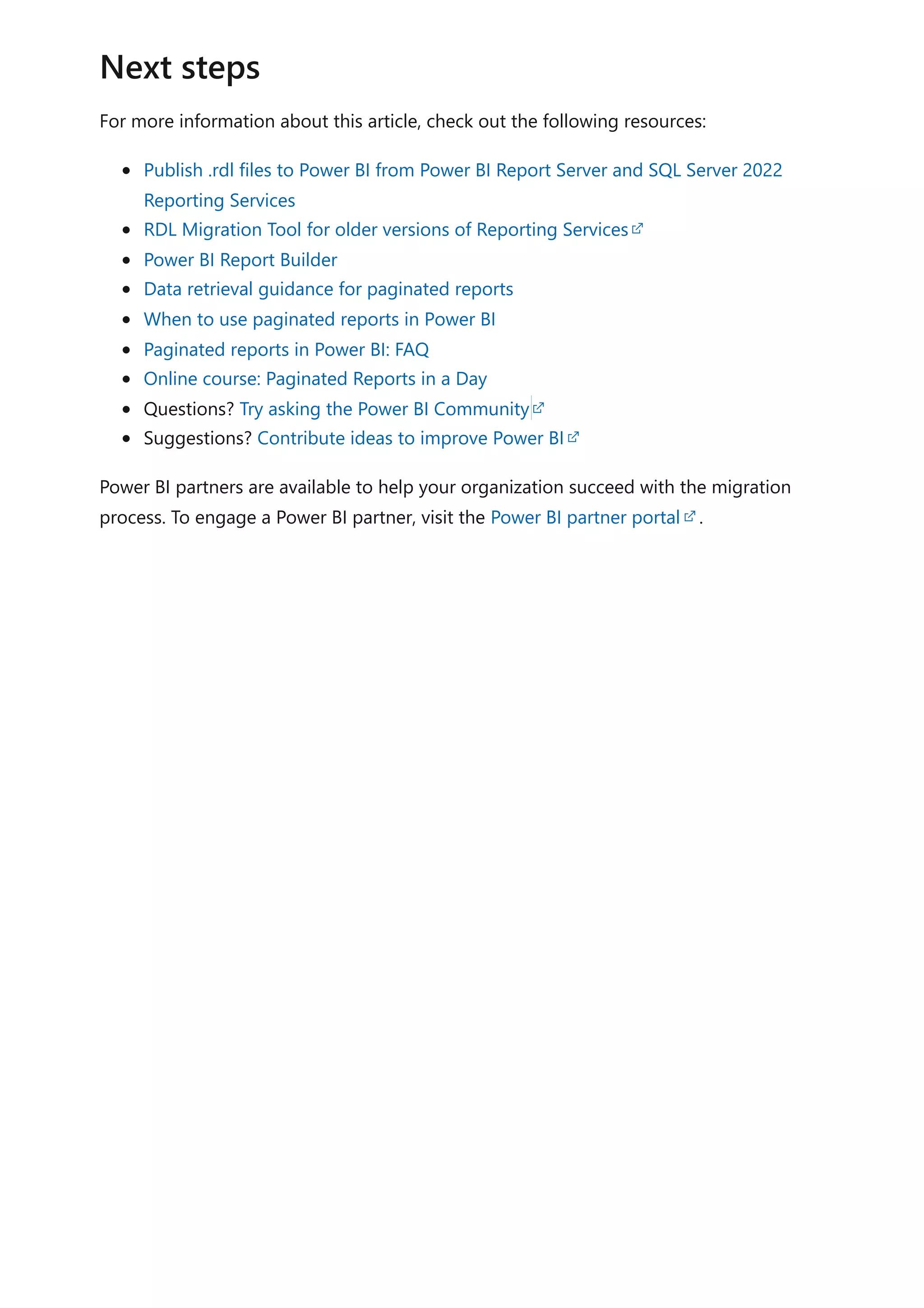
For more information related to this article, check out the following resources:
Auto date/time in Power BI Desktop
Auto date/time guidance in Power BI Desktop
Set and use date tables in Power BI Desktop
Self-service data prep in Power BI
CALENDAR function (DAX)
CALENDARAUTO function (DAX)
Questions? Try asking the Power BI Community
Tip
For more information about creating calculated tables, including an example of
how to create a date table, work through the Add calculated tables and columns
to Power BI Desktop models learning module.
Clone with DAX
Next steps](https://image.slidesharecdn.com/docpower-bi-guidance-230227102019-b6273799/75/DOC-Power-Bi-Guidance-pdf-43-2048.jpg)


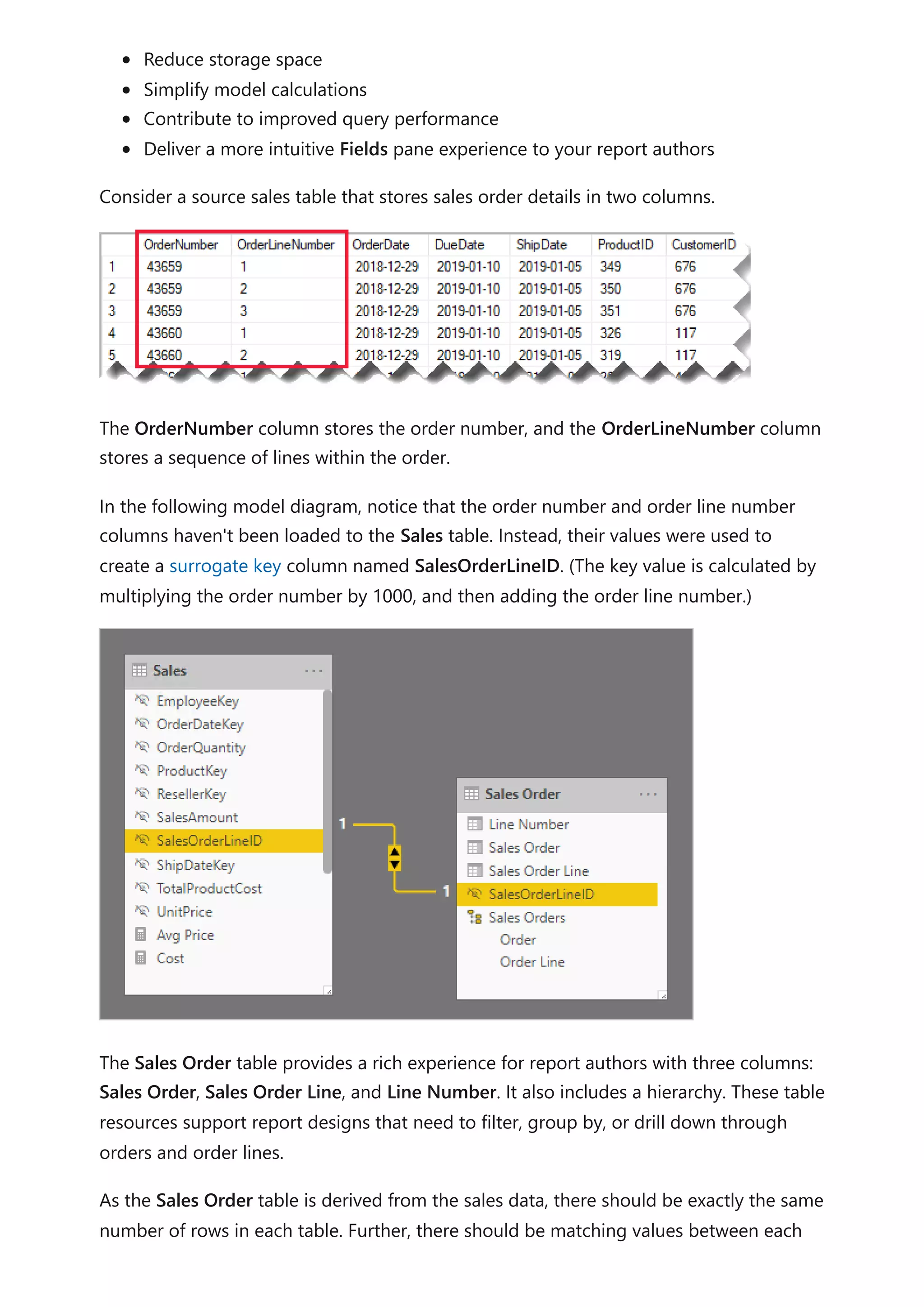
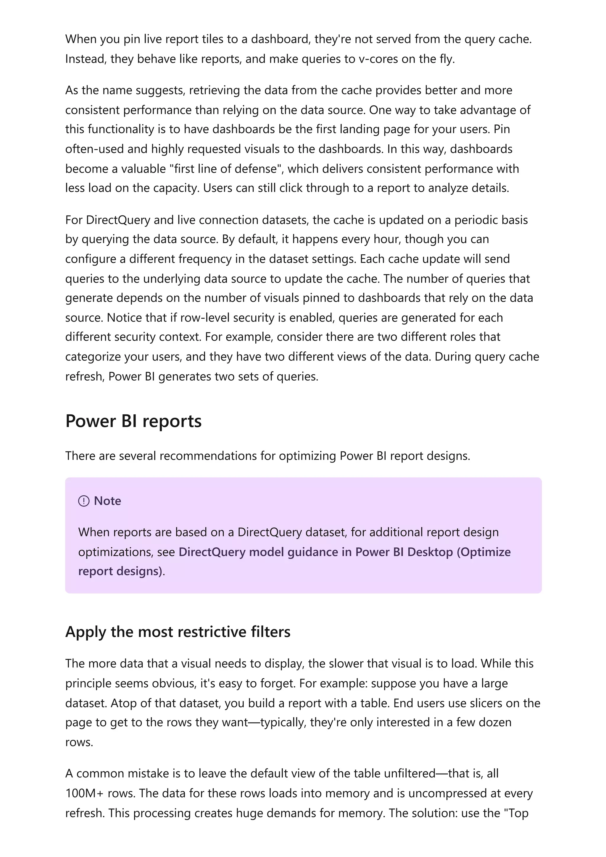
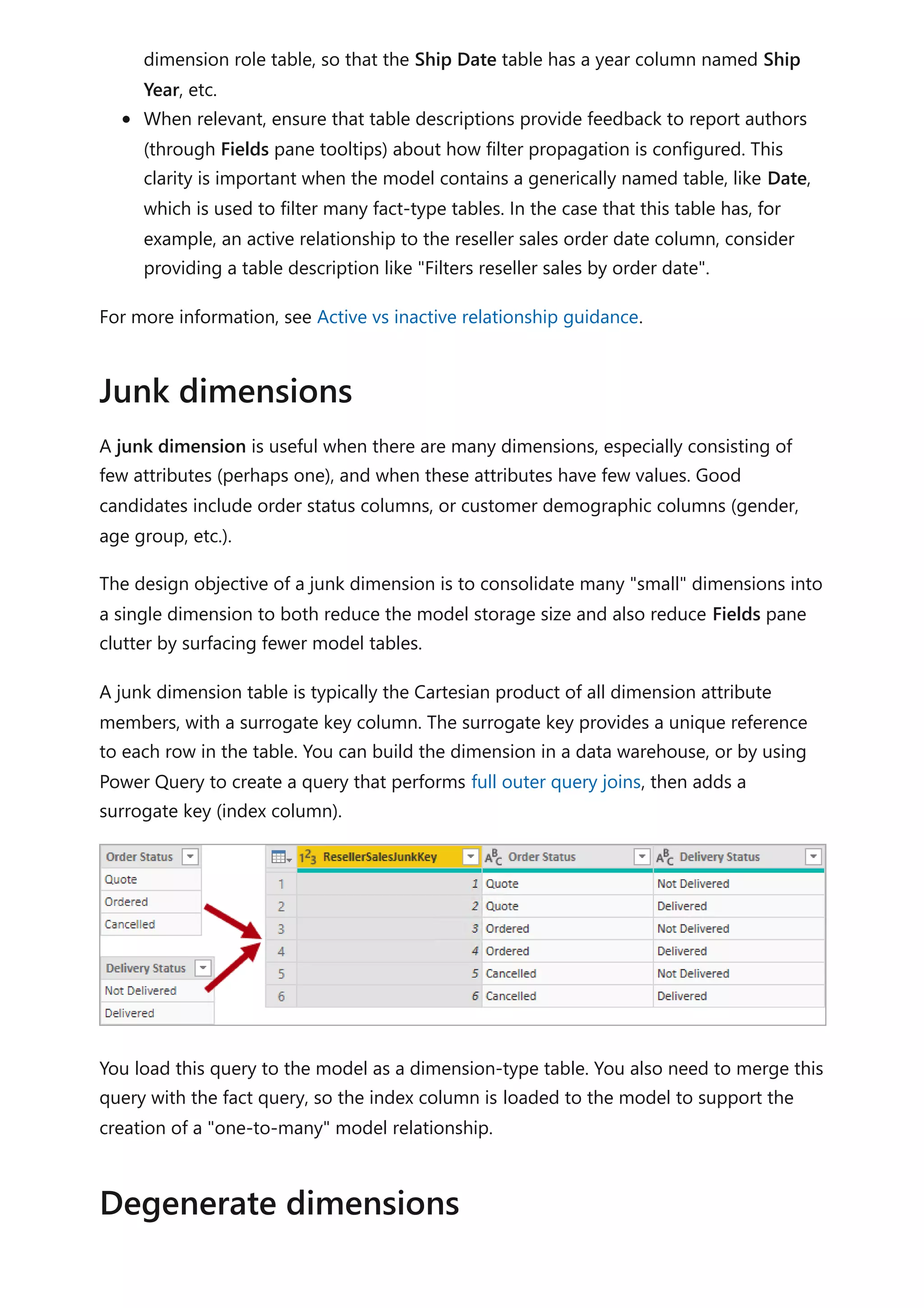
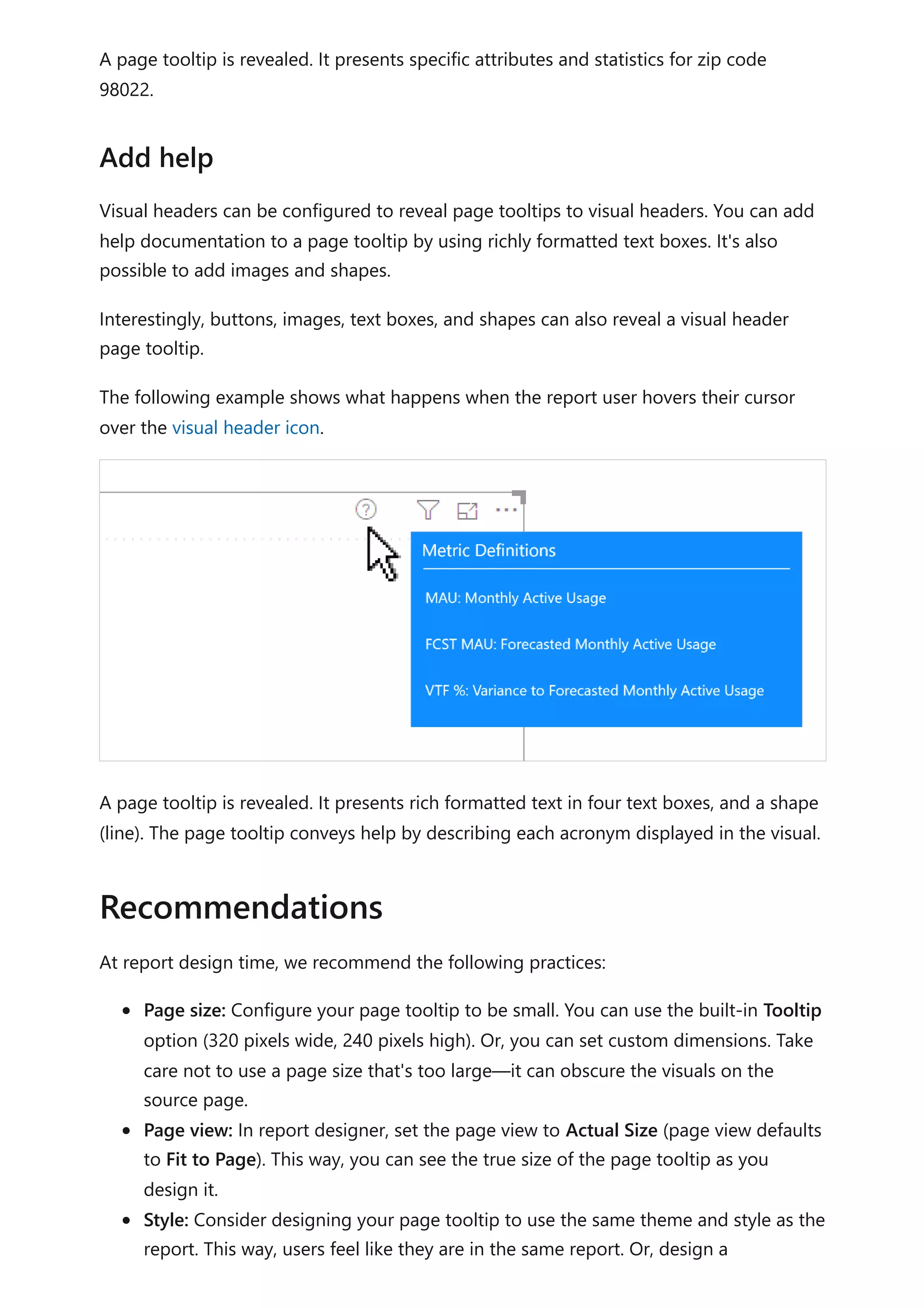
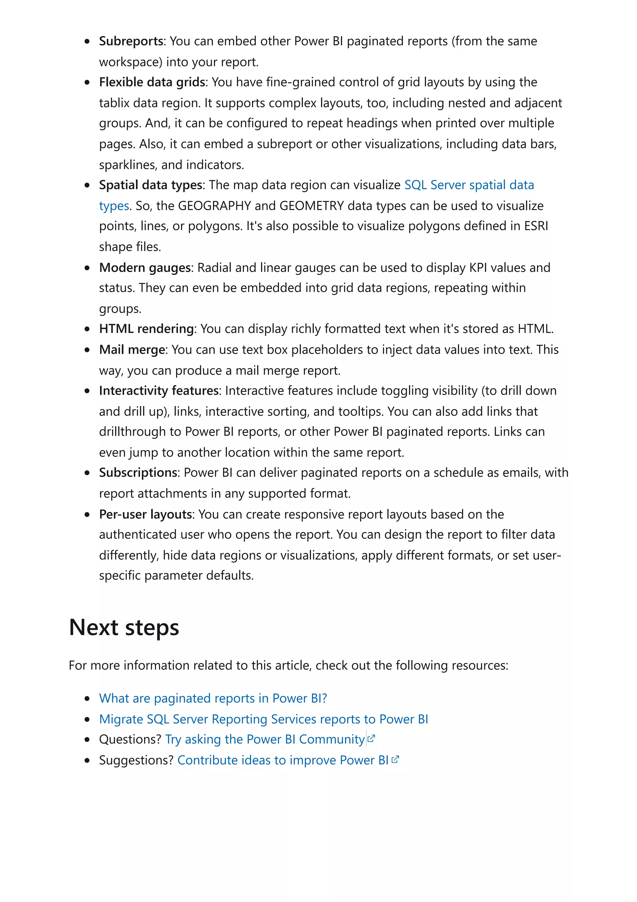
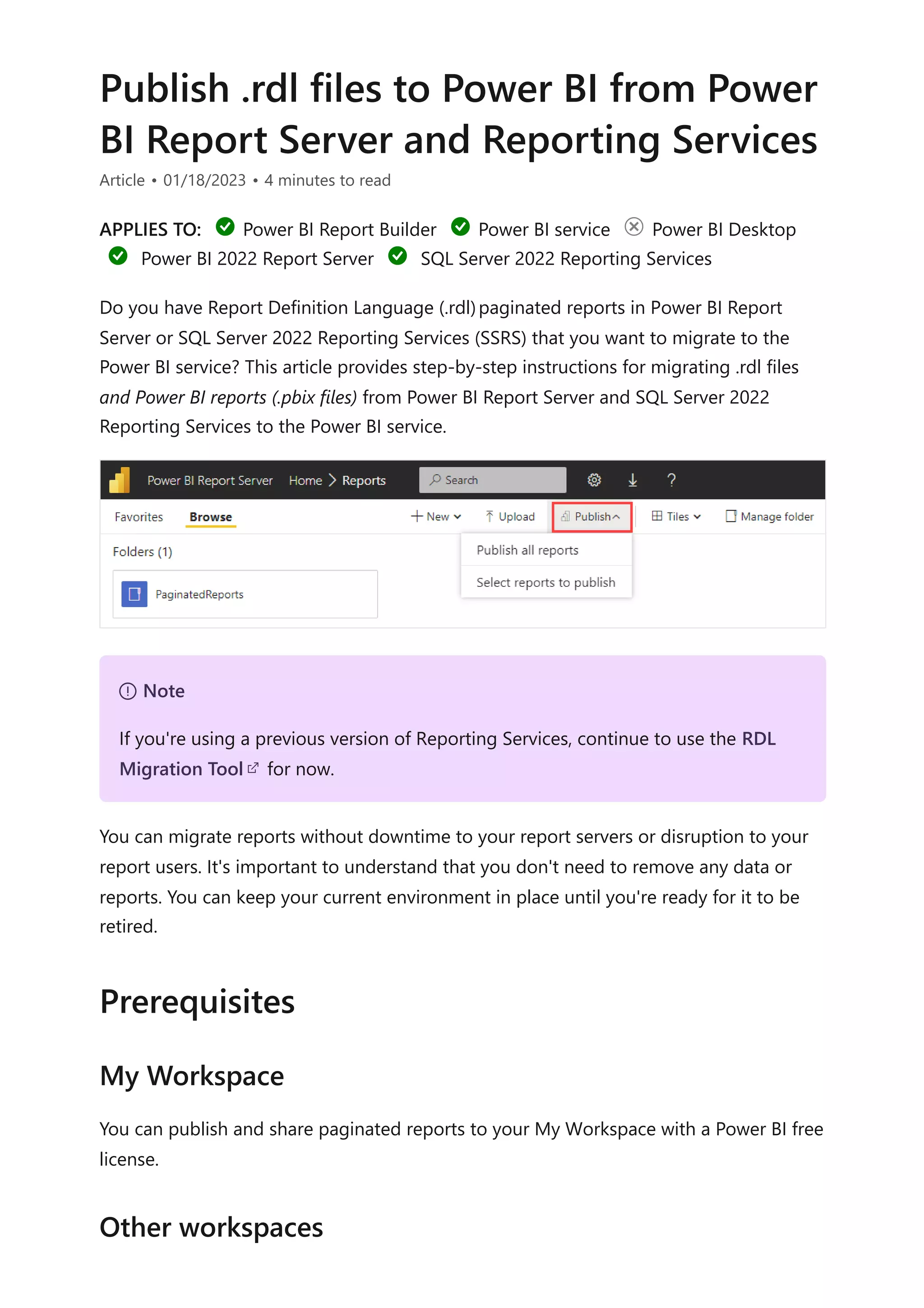
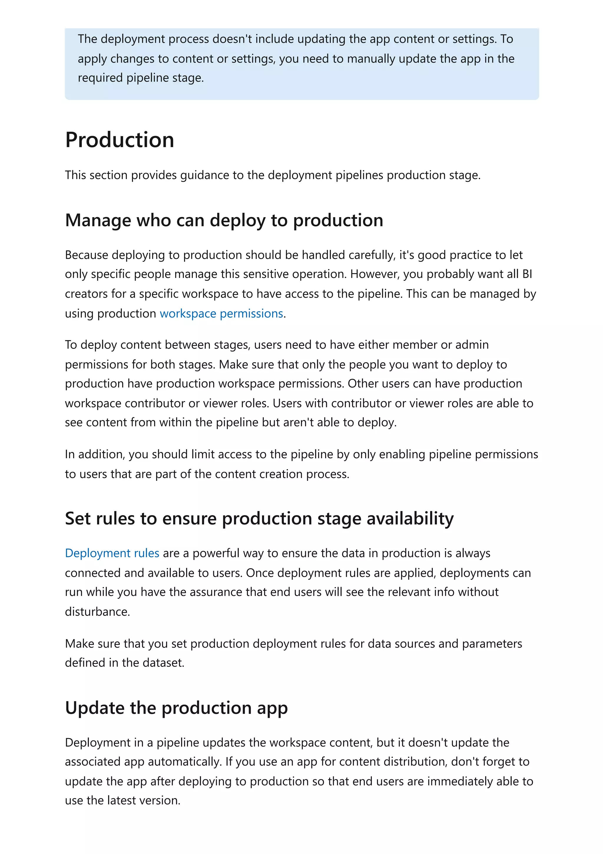
![matching rows of the second query. Expand all required columns of the second
query into the first query.
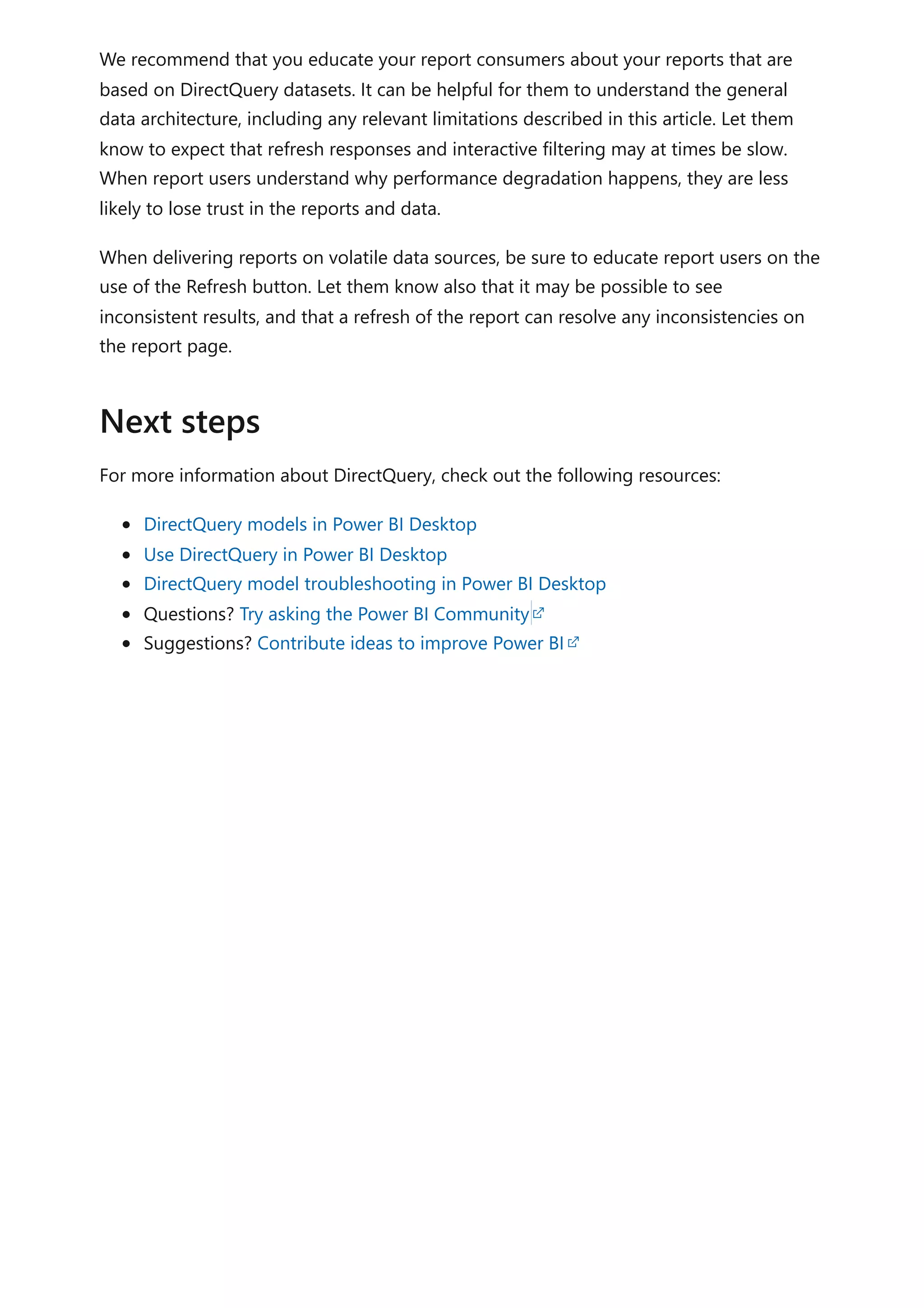
2. Disable query load: Be sure to disable the load of the second query. This way, it
won't load its result as a model table. This configuration reduces the data model
storage size, and helps to unclutter the Fields pane.
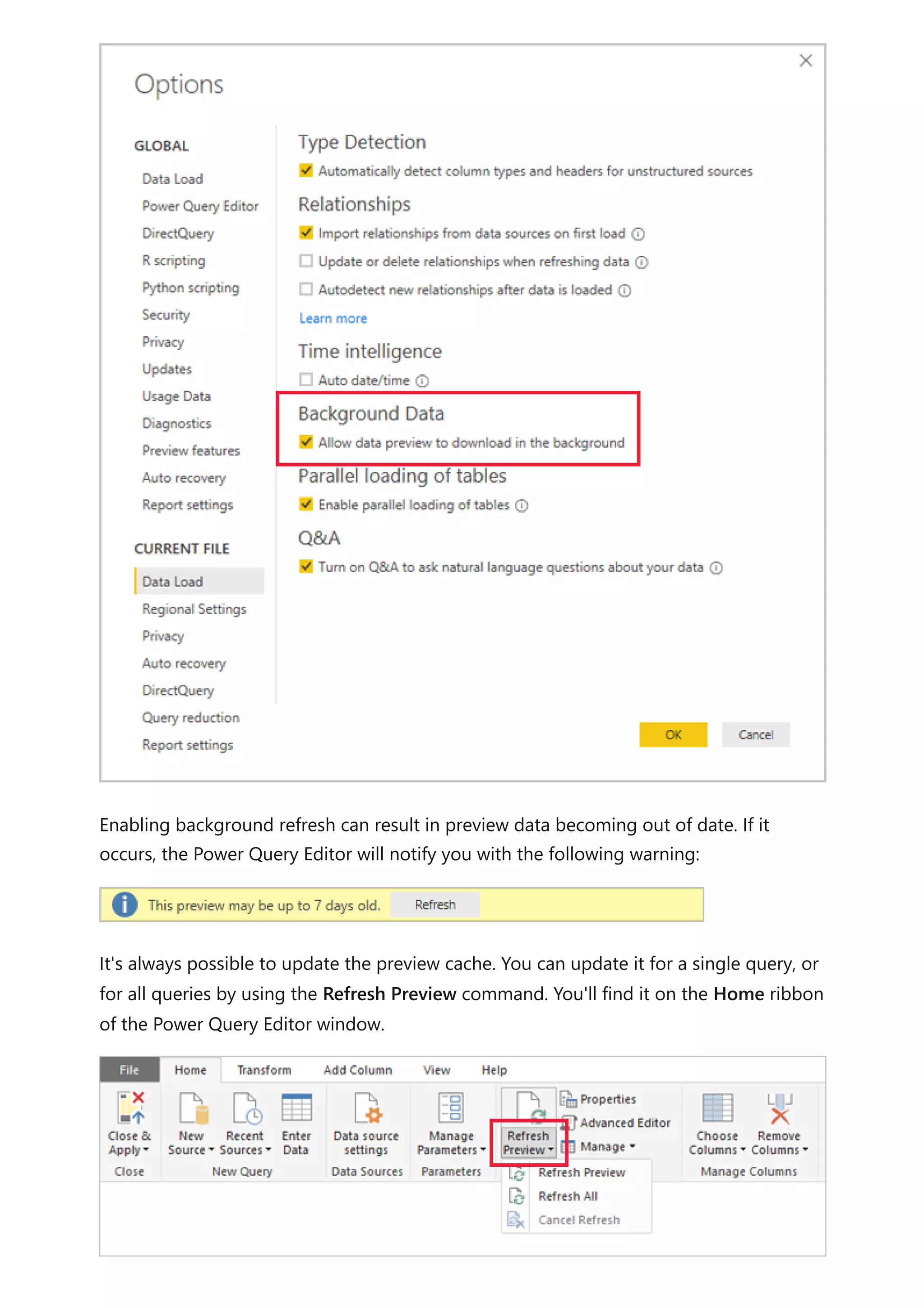
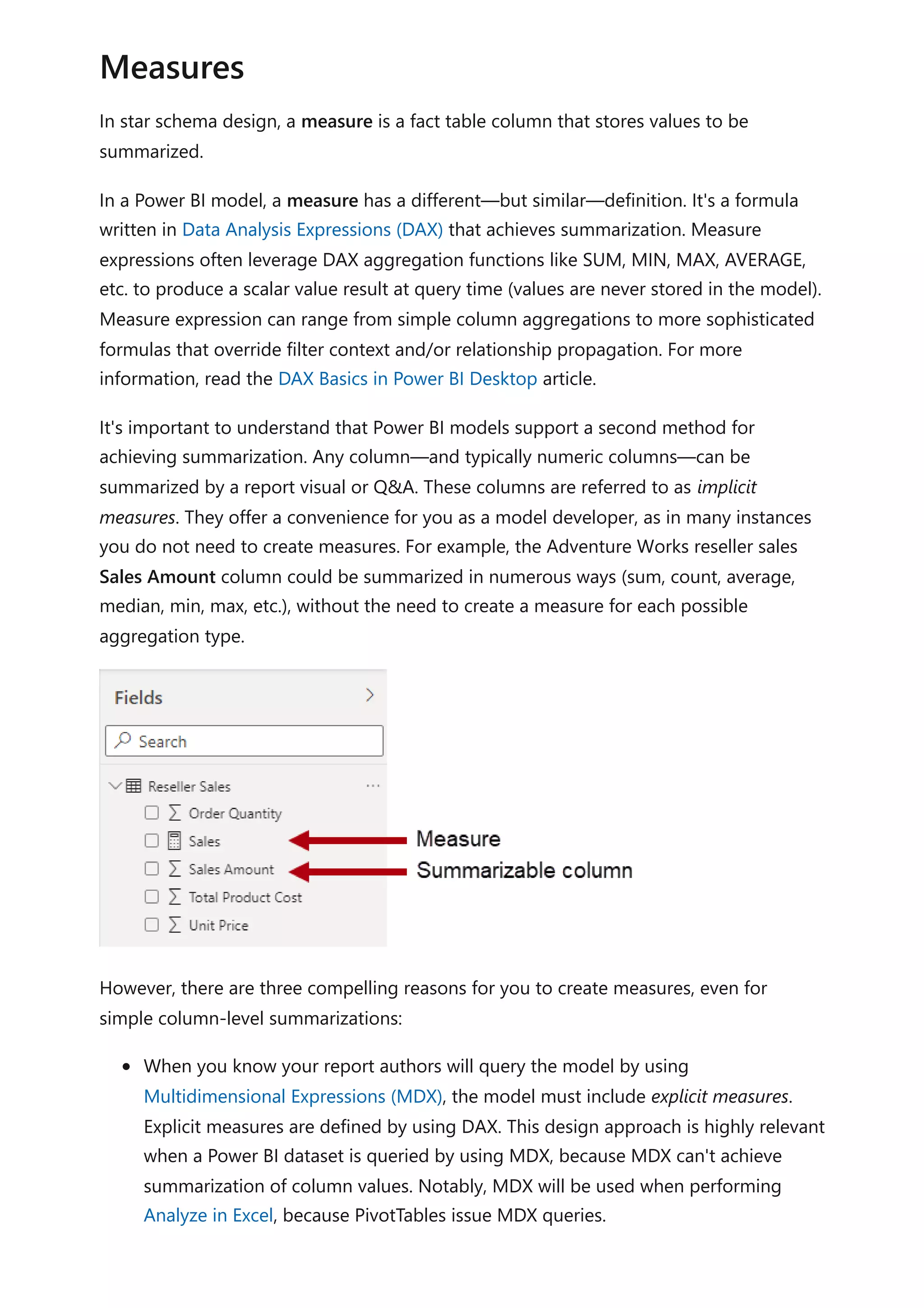
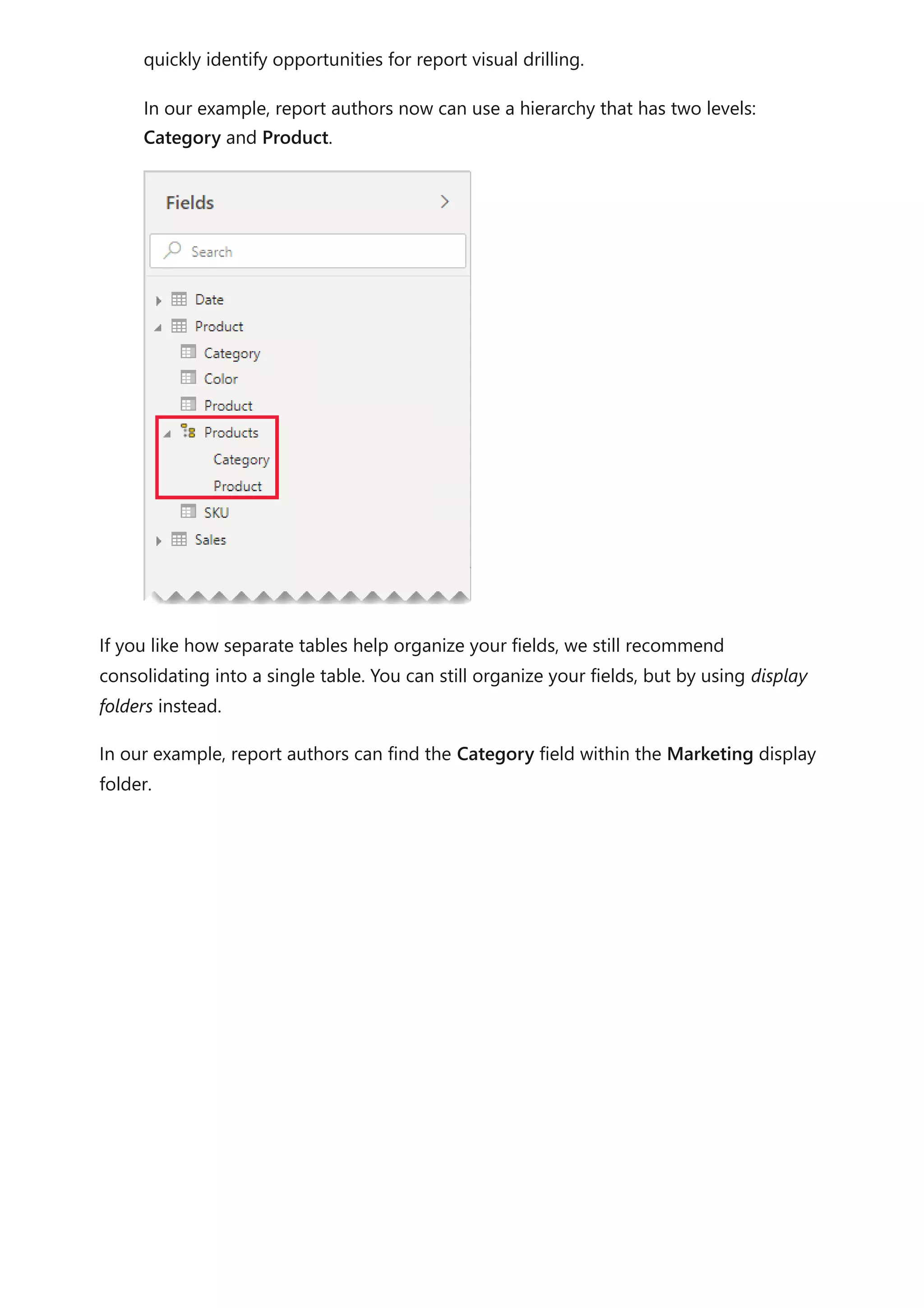
In our example, report authors now find a single table named Product in the Fields
pane. It contains all product-related fields.
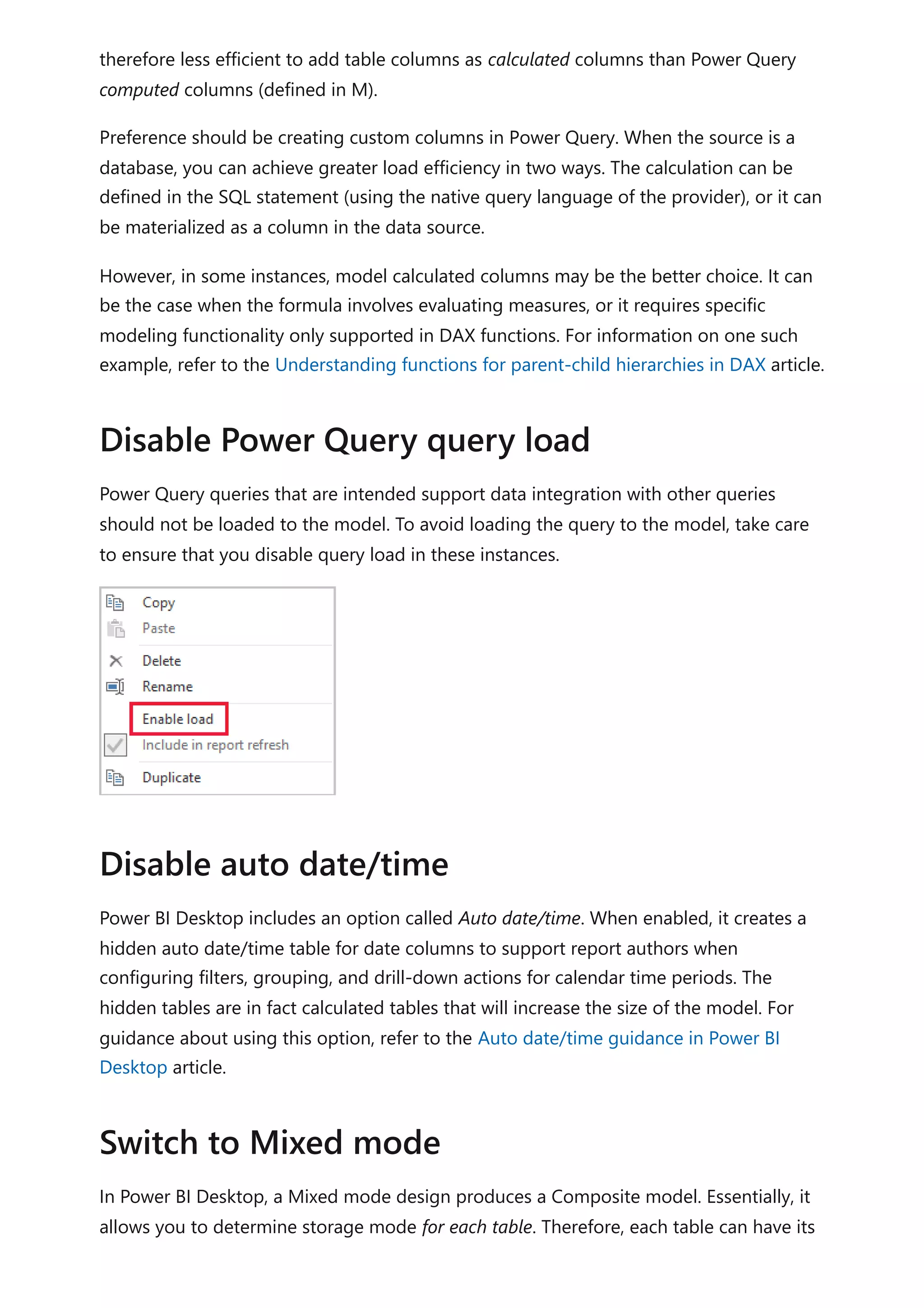
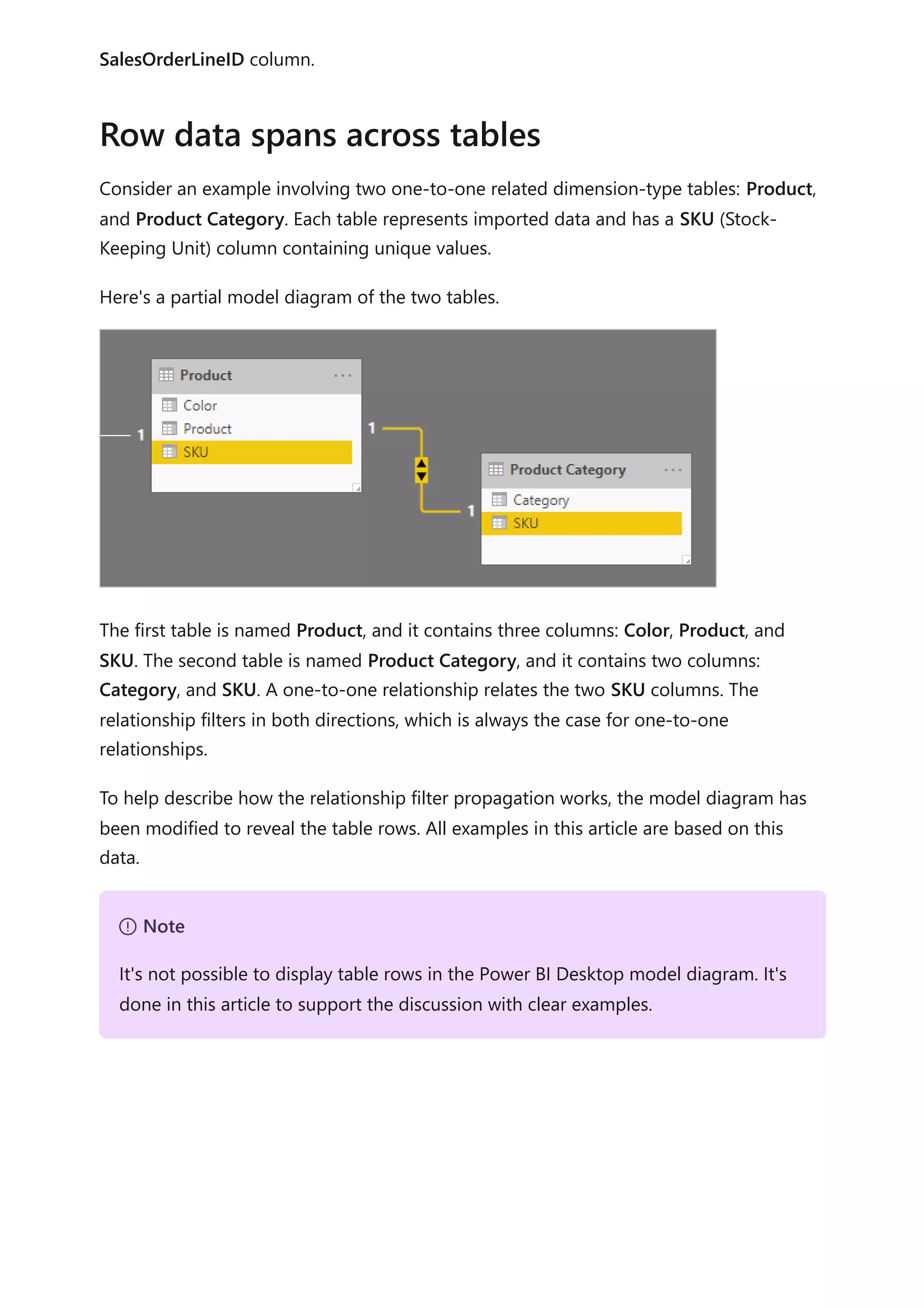
3. Replace missing values: If the second query has unmatched rows, NULLs will
appear in the columns introduced from it. When appropriate, consider replacing
NULLs with a token value. Replacing missing values is especially important when
report authors filter or group by the column values, as BLANKs could appear in
report visuals.
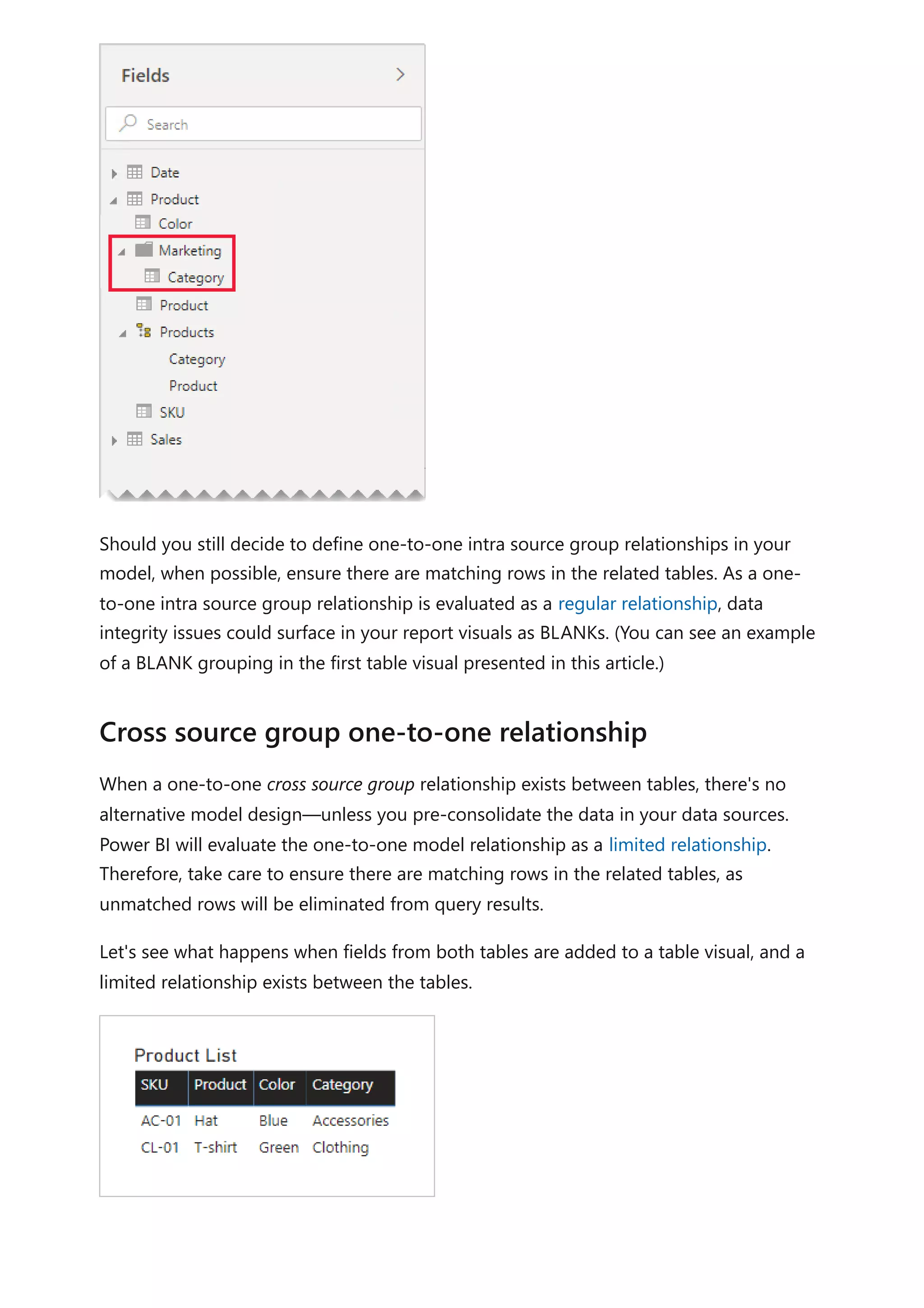
In the following table visual, notice that the category for product SKU CL-02 now
reads [Undefined]. In the query, null categories were replaced with this token text
value.
4. Create hierarchies: If relationships exist between the columns of the now-
consolidated table, consider creating hierarchies. This way, report authors will](https://image.slidesharecdn.com/docpower-bi-guidance-230227102019-b6273799/75/DOC-Power-Bi-Guidance-pdf-53-2048.jpg)
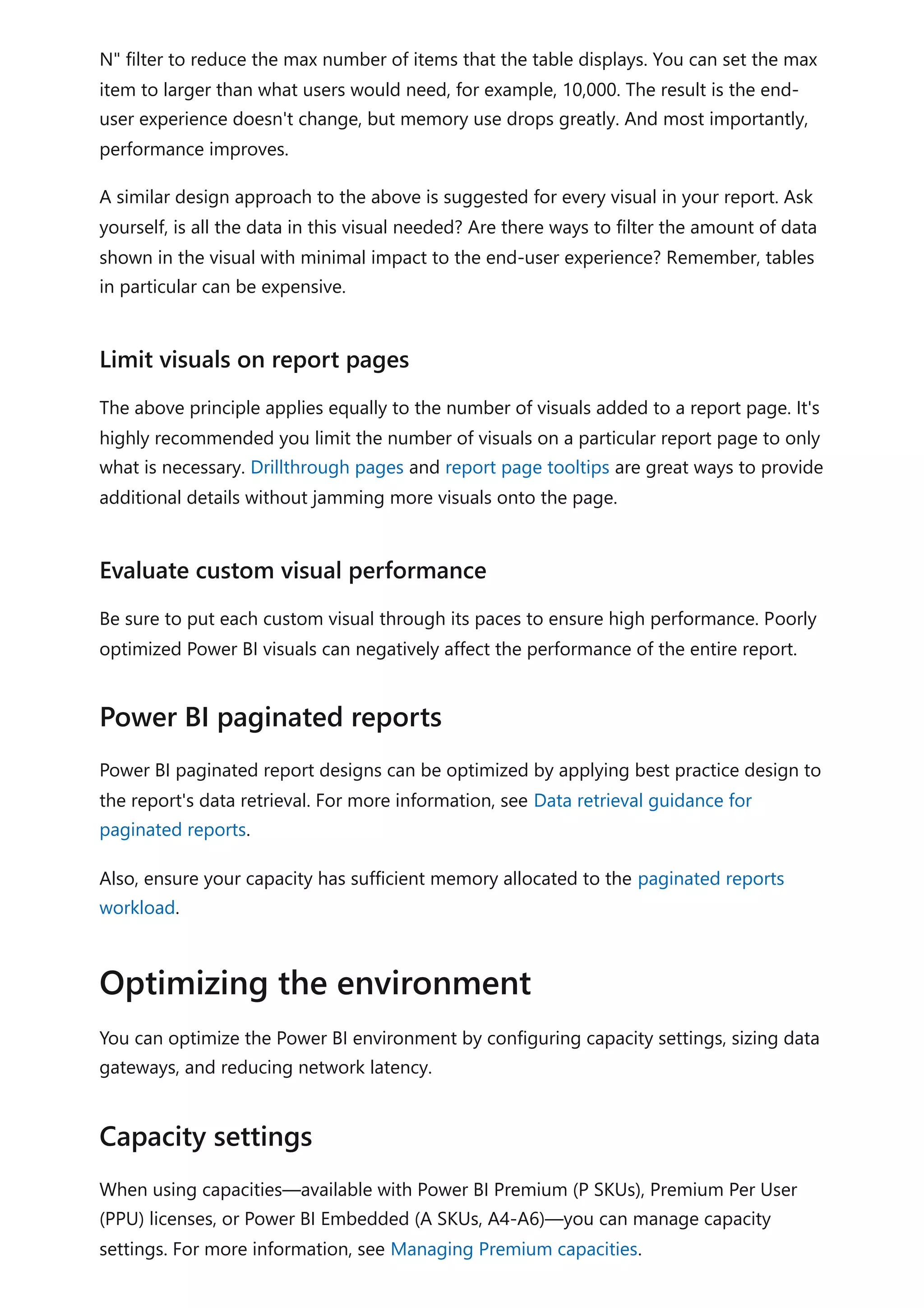
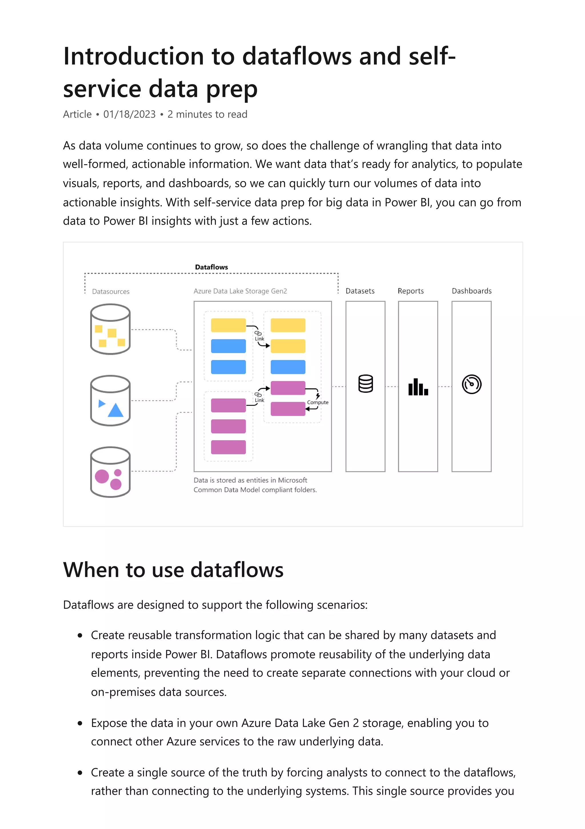
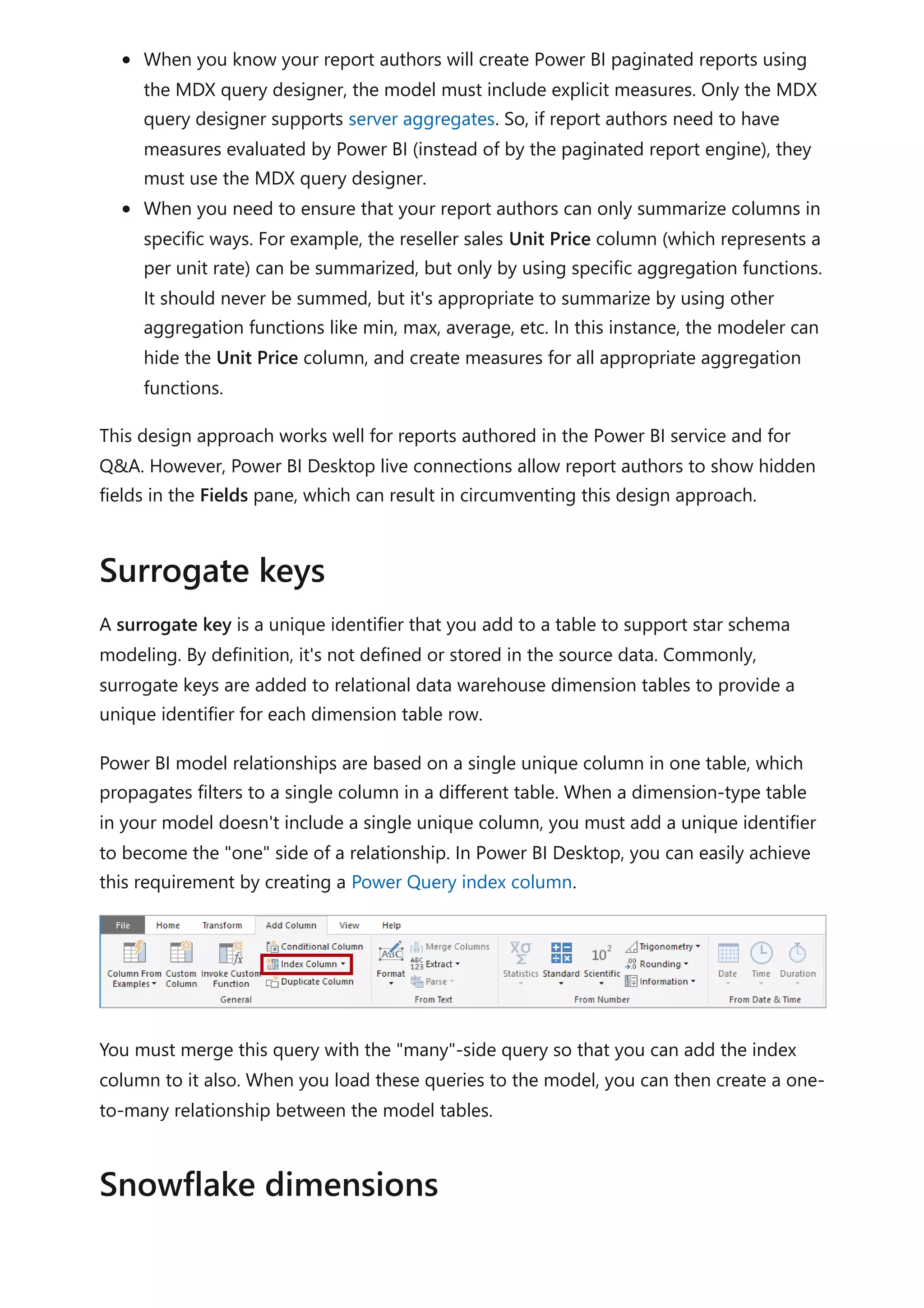
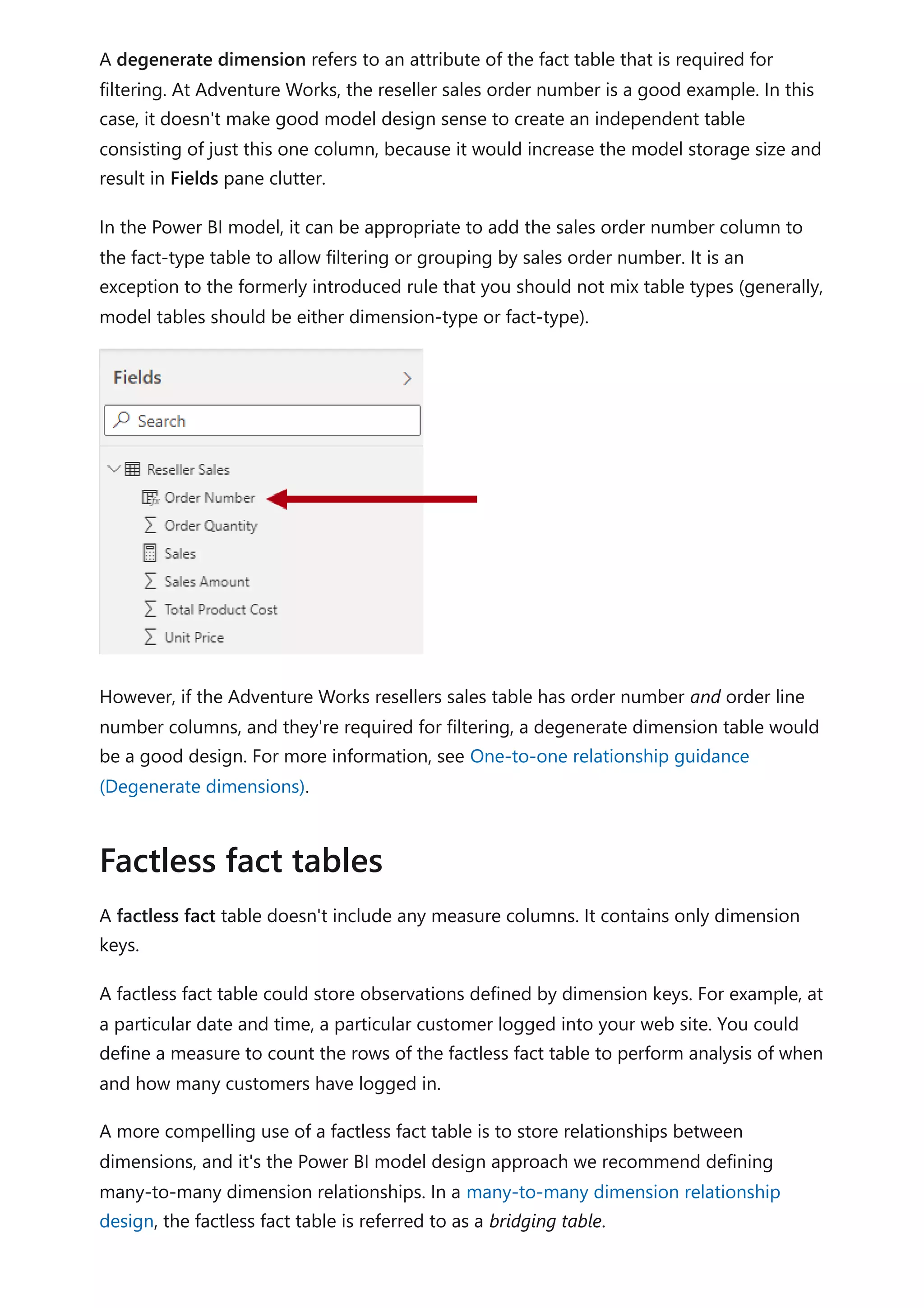
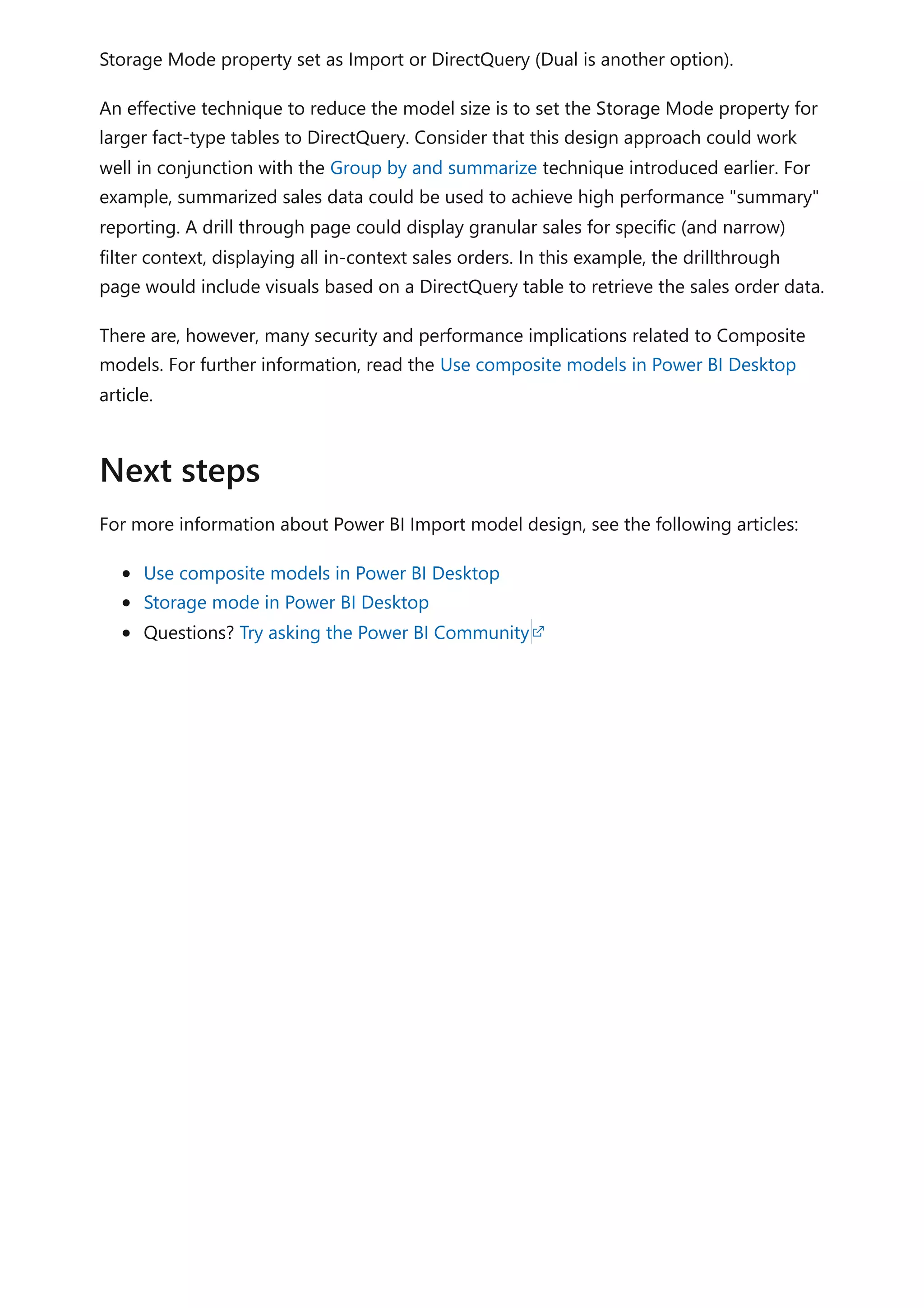
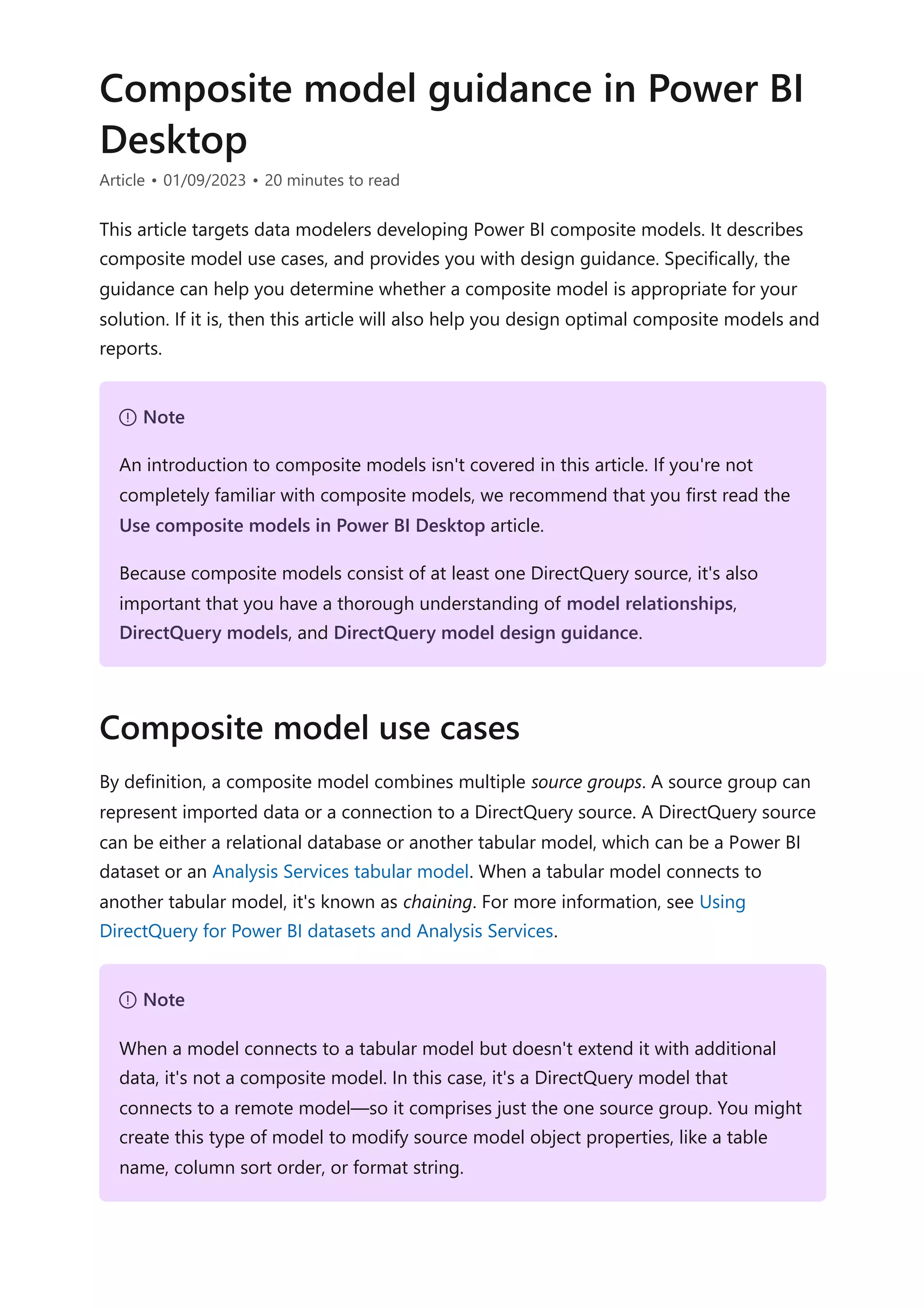
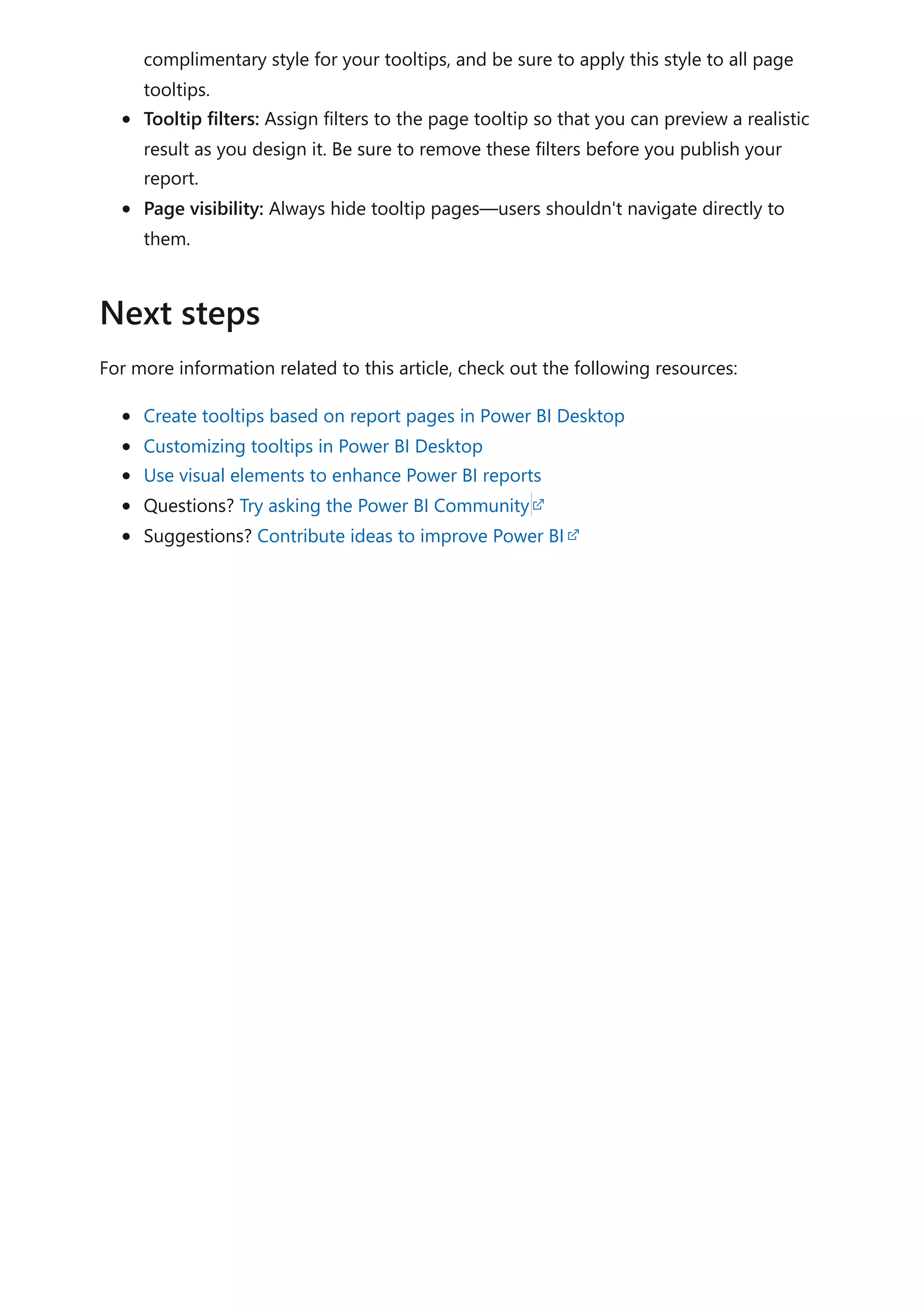
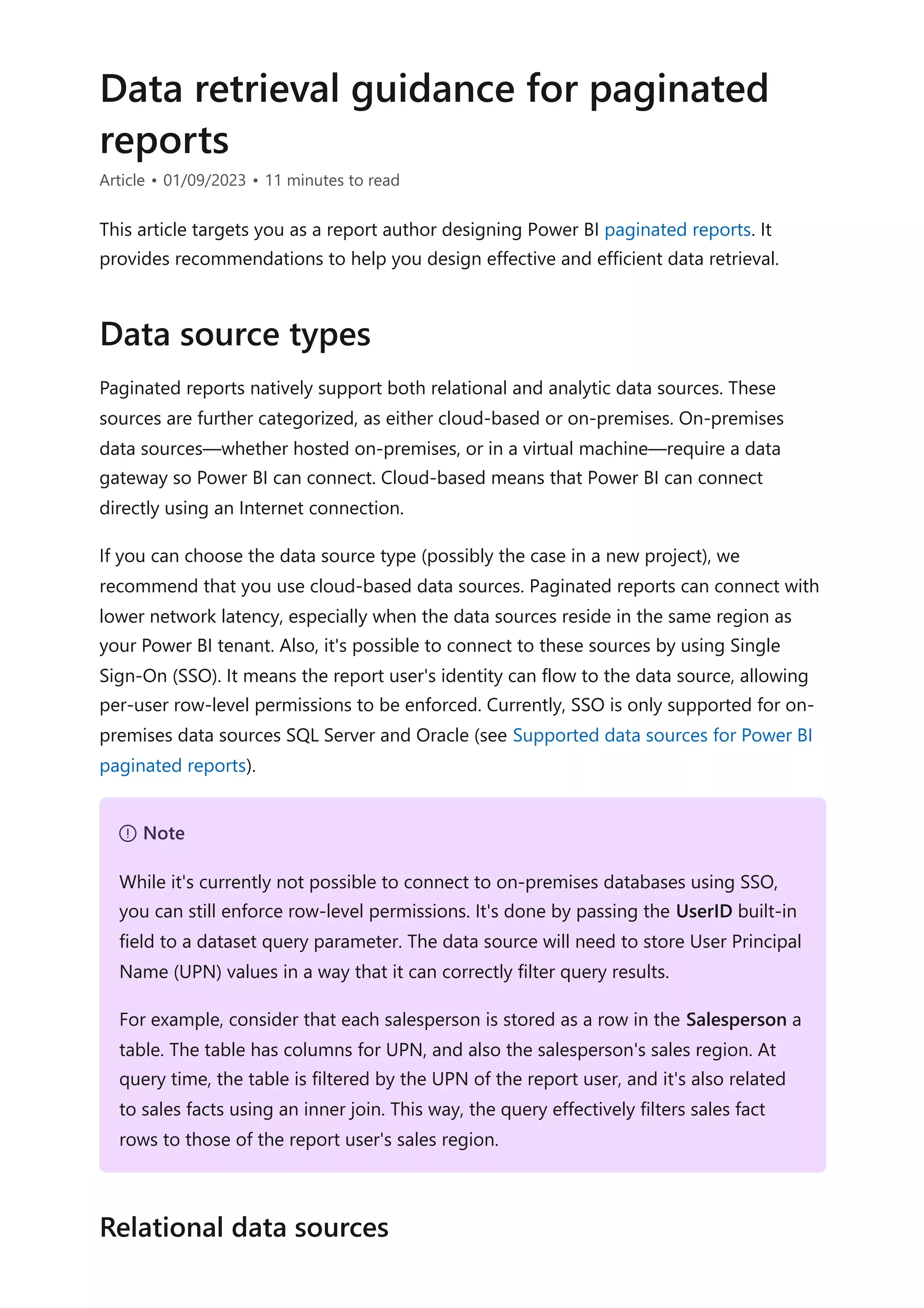
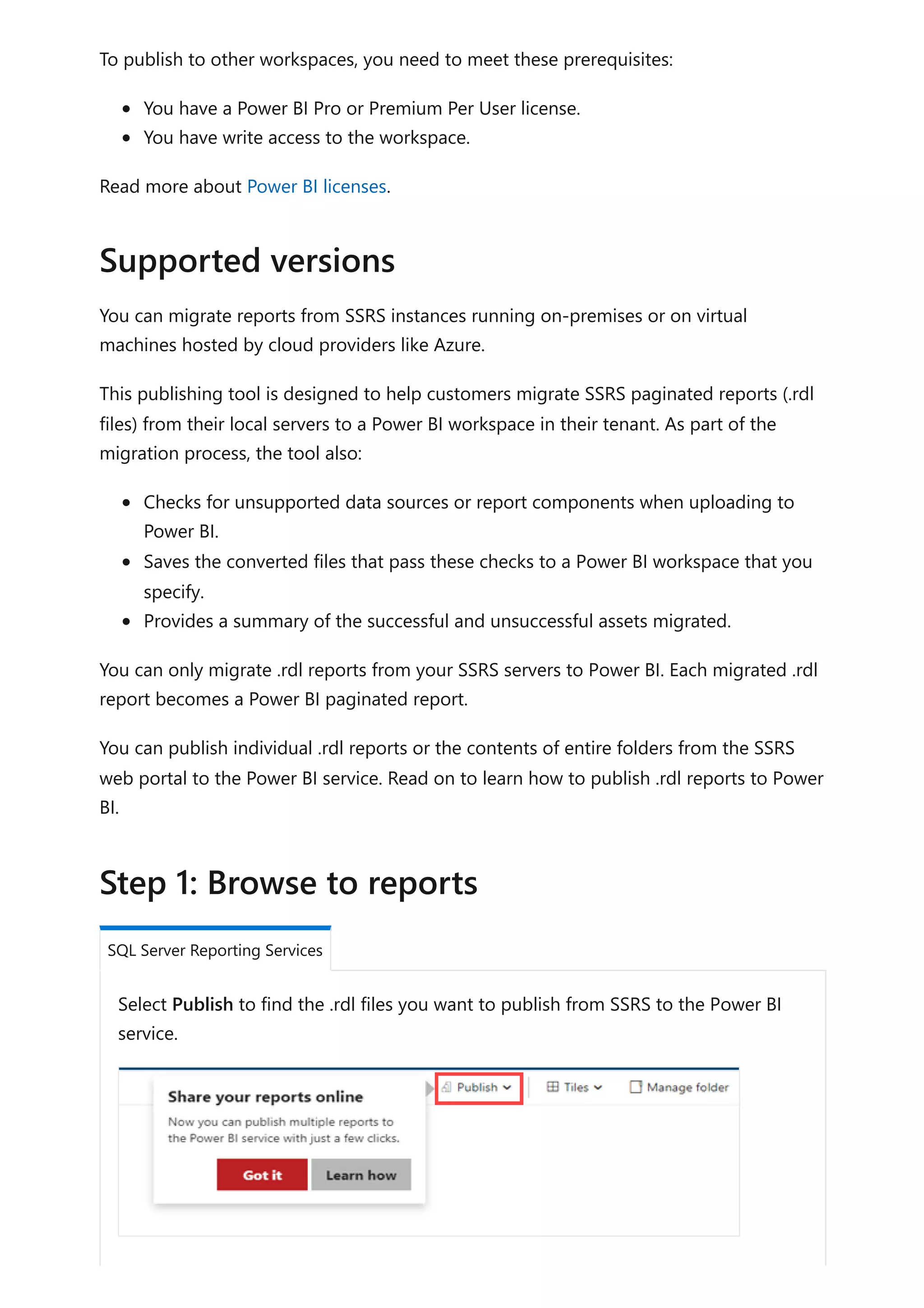
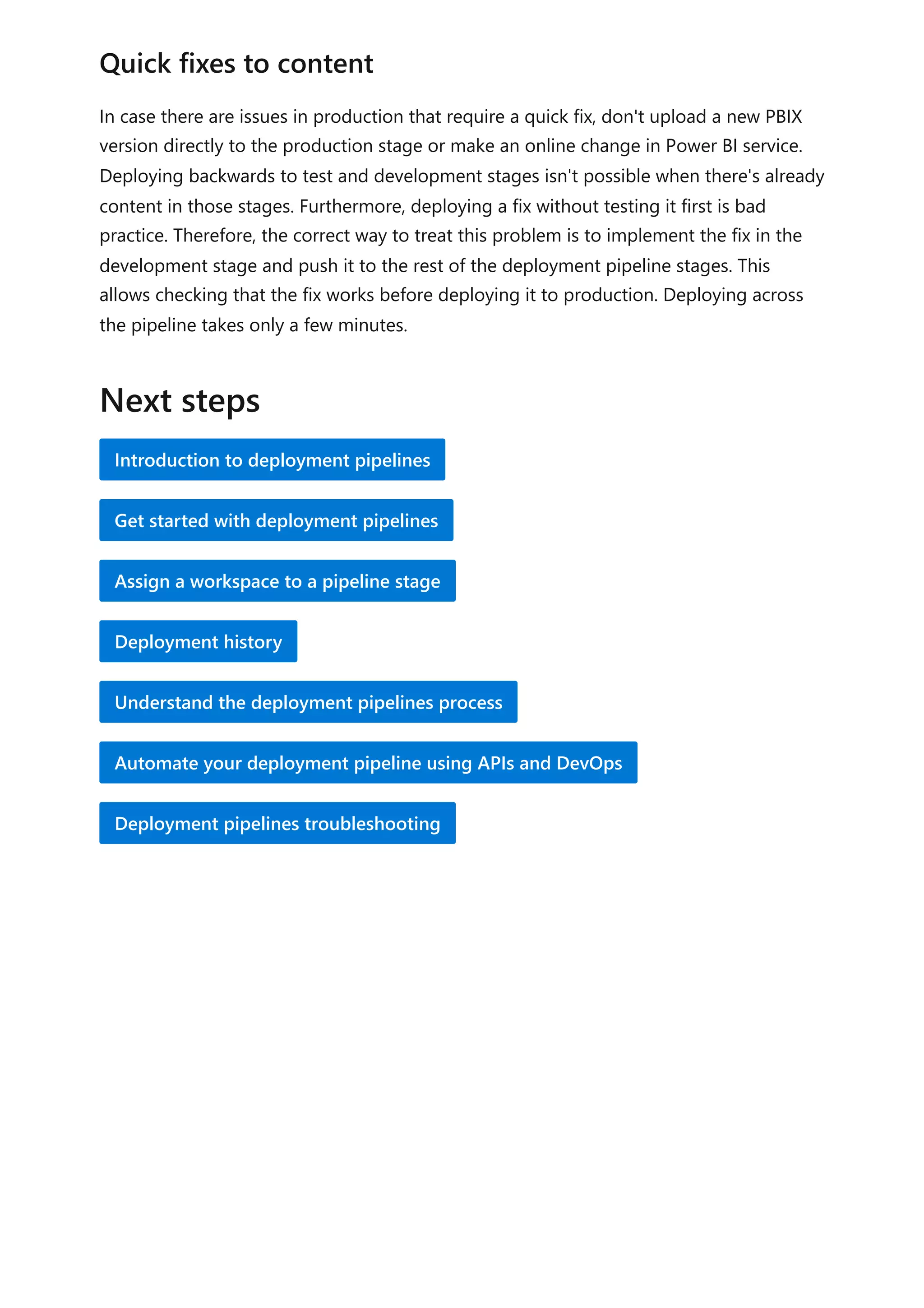
![Consider the following measure definition that uses the ISFILTERED DAX function. It only
returns a value when the Date or Month columns aren't filtered.
DAX
The following matrix visual now uses the Target Quantity measure. It shows that all
monthly target quantities are BLANK.
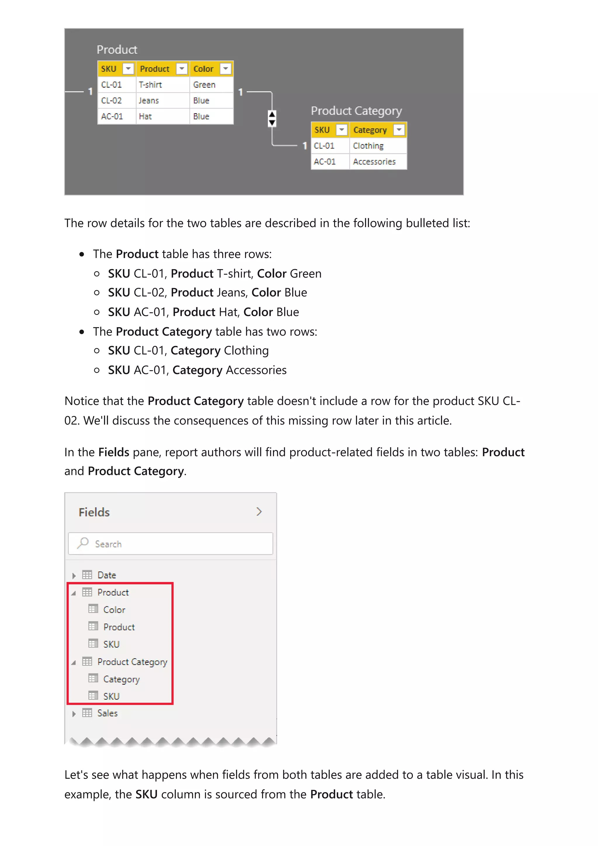
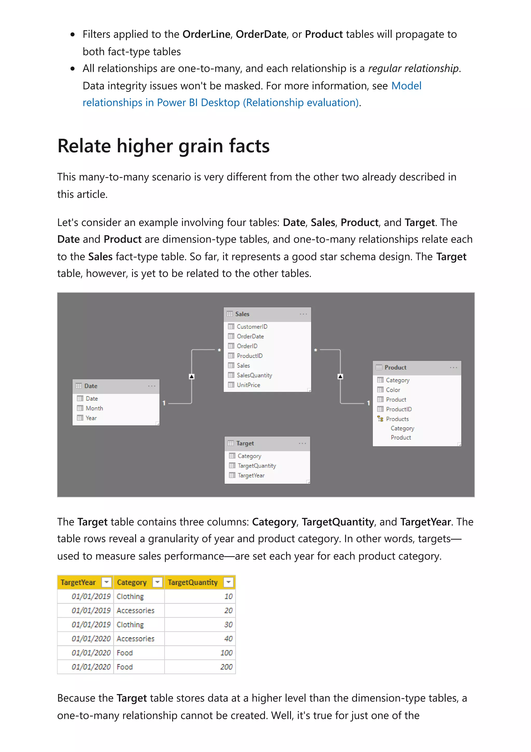
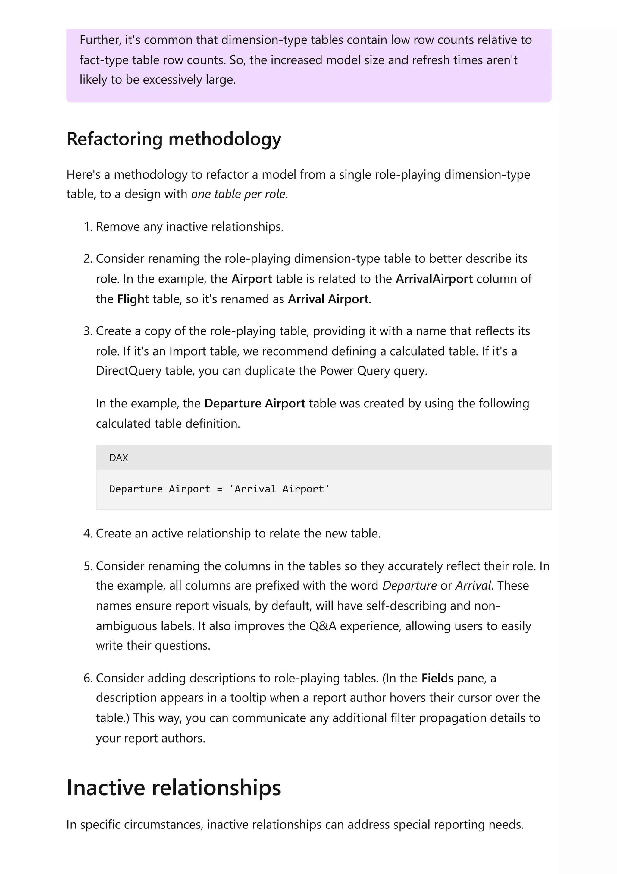
A different design approach is required when relating a non-date column from a
dimension-type table to a fact-type table (and it's at a higher grain than the dimension-
type table).
The Category columns (from both the Product and Target tables) contains duplicate
values. So, there's no "one" for a one-to-many relationship. In this case, you'll need to
create a many-to-many relationship. The relationship should propagate filters in a single
direction, from the dimension-type table to the fact-type table.
Target Quantity =
IF(
NOT ISFILTERED('Date'[Date])
&& NOT ISFILTERED('Date'[Month]),
SUM(Target[TargetQuantity])
)
Relate higher grain (non-date)](https://image.slidesharecdn.com/docpower-bi-guidance-230227102019-b6273799/75/DOC-Power-Bi-Guidance-pdf-68-2048.jpg)
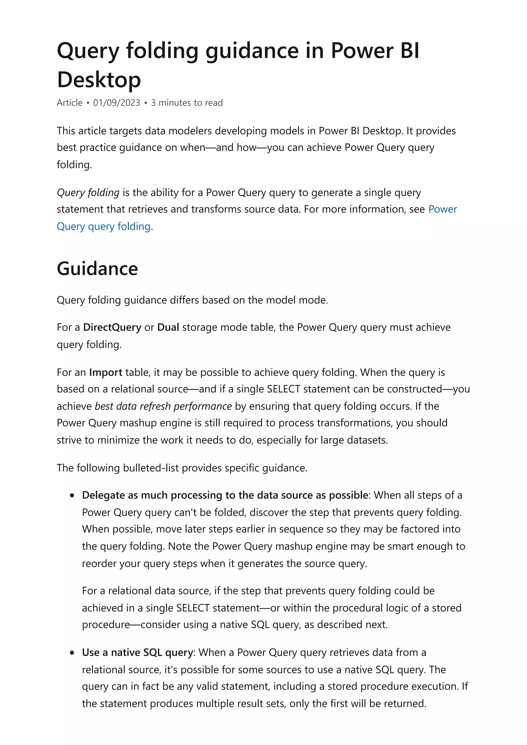
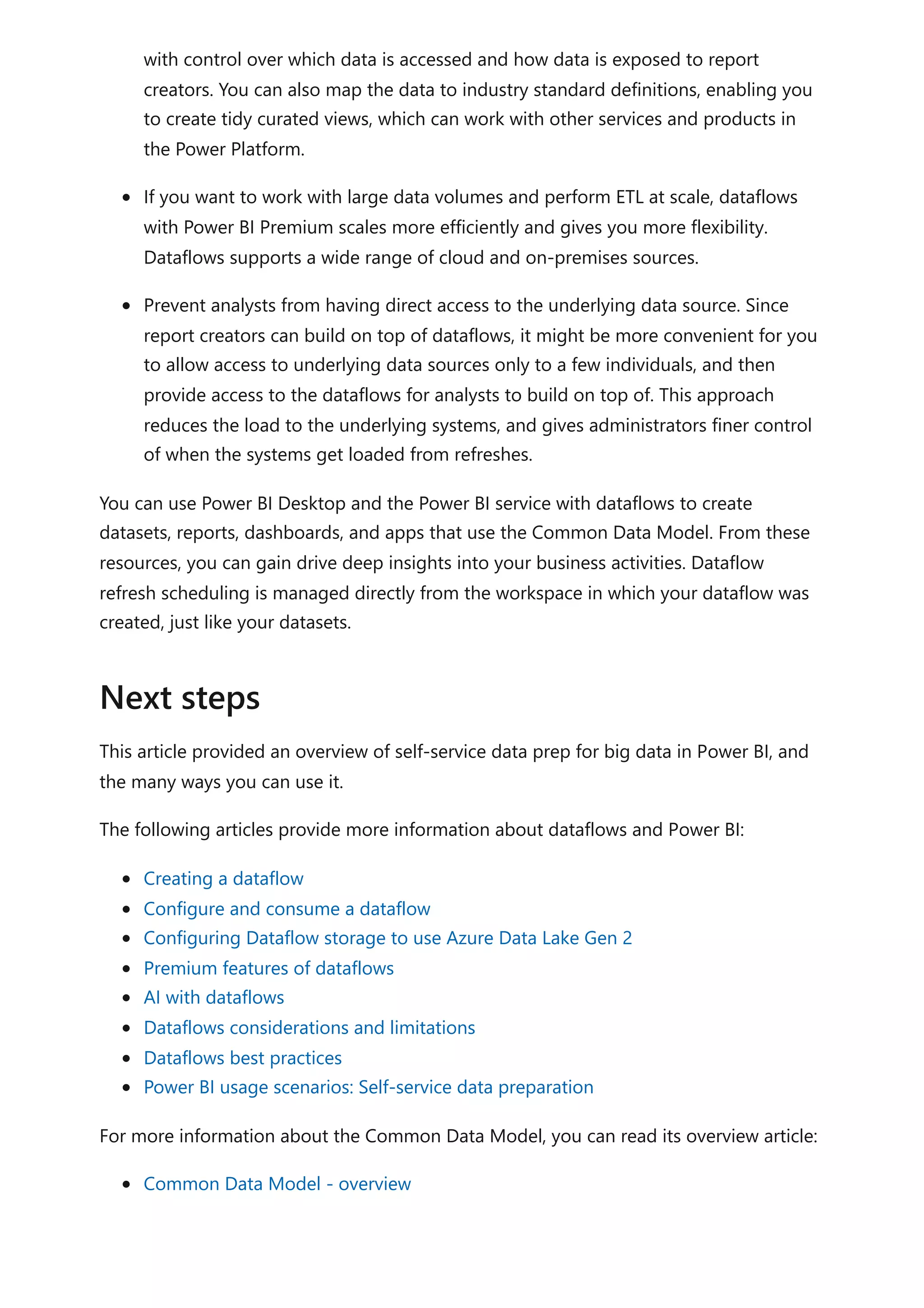
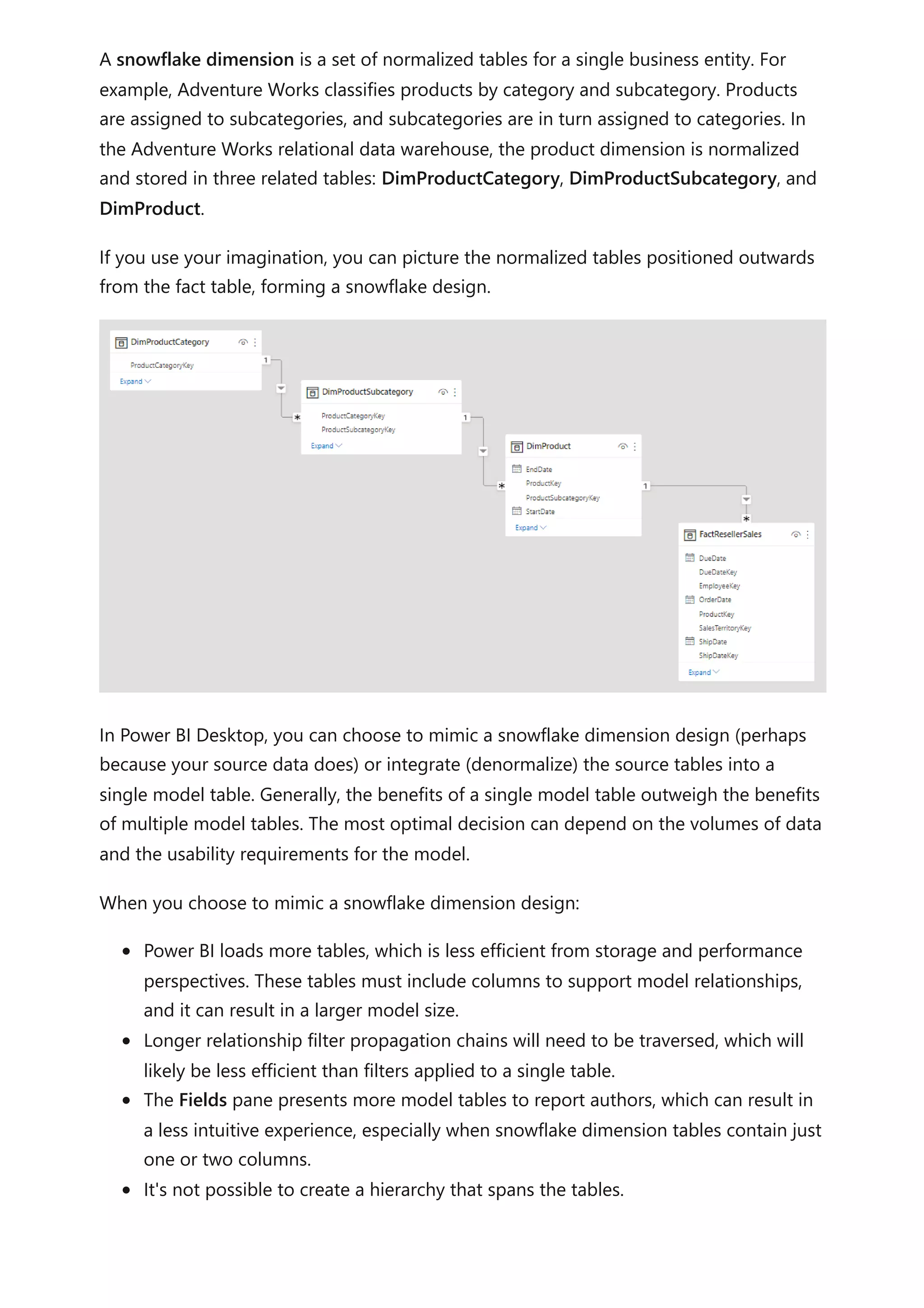
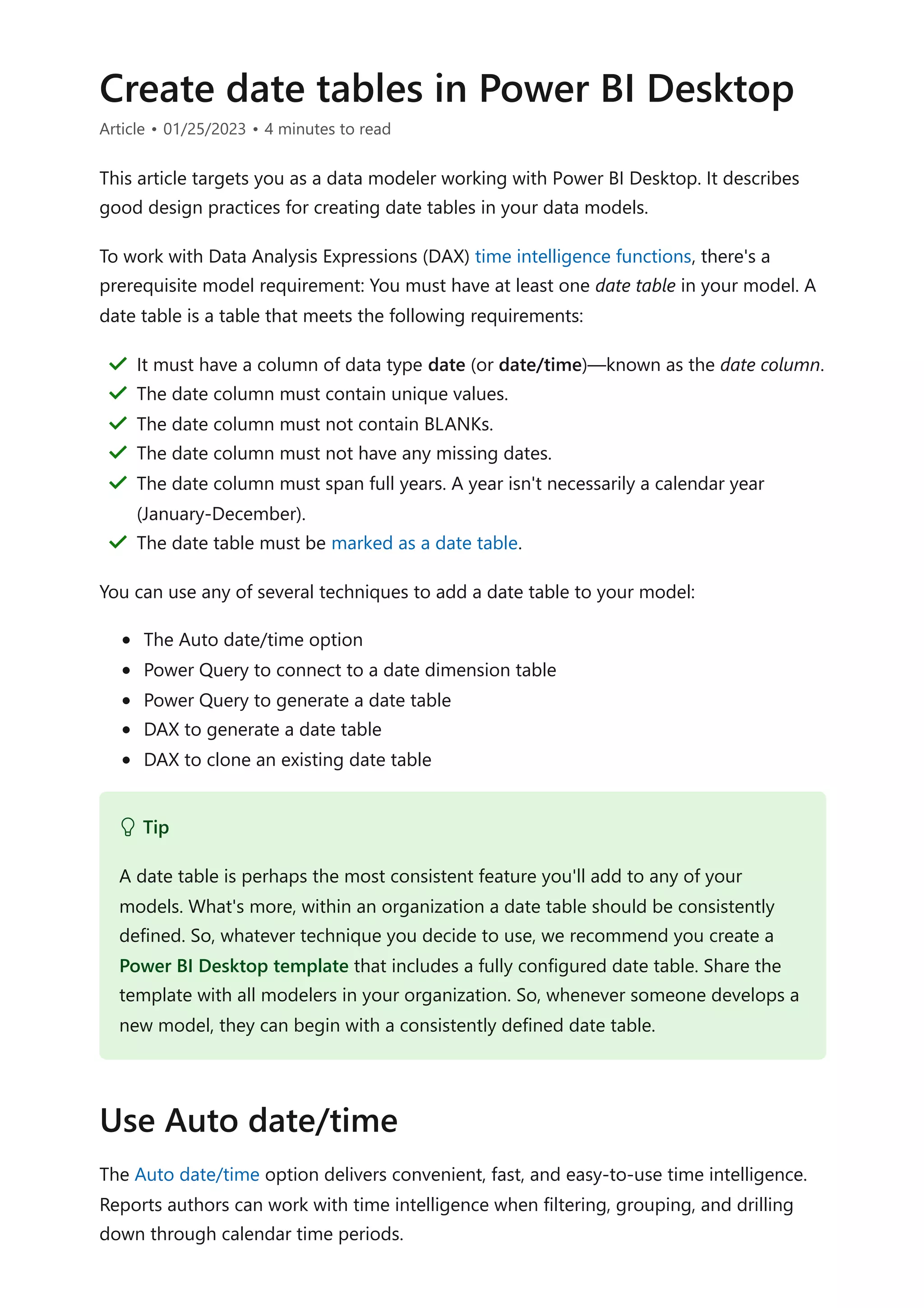
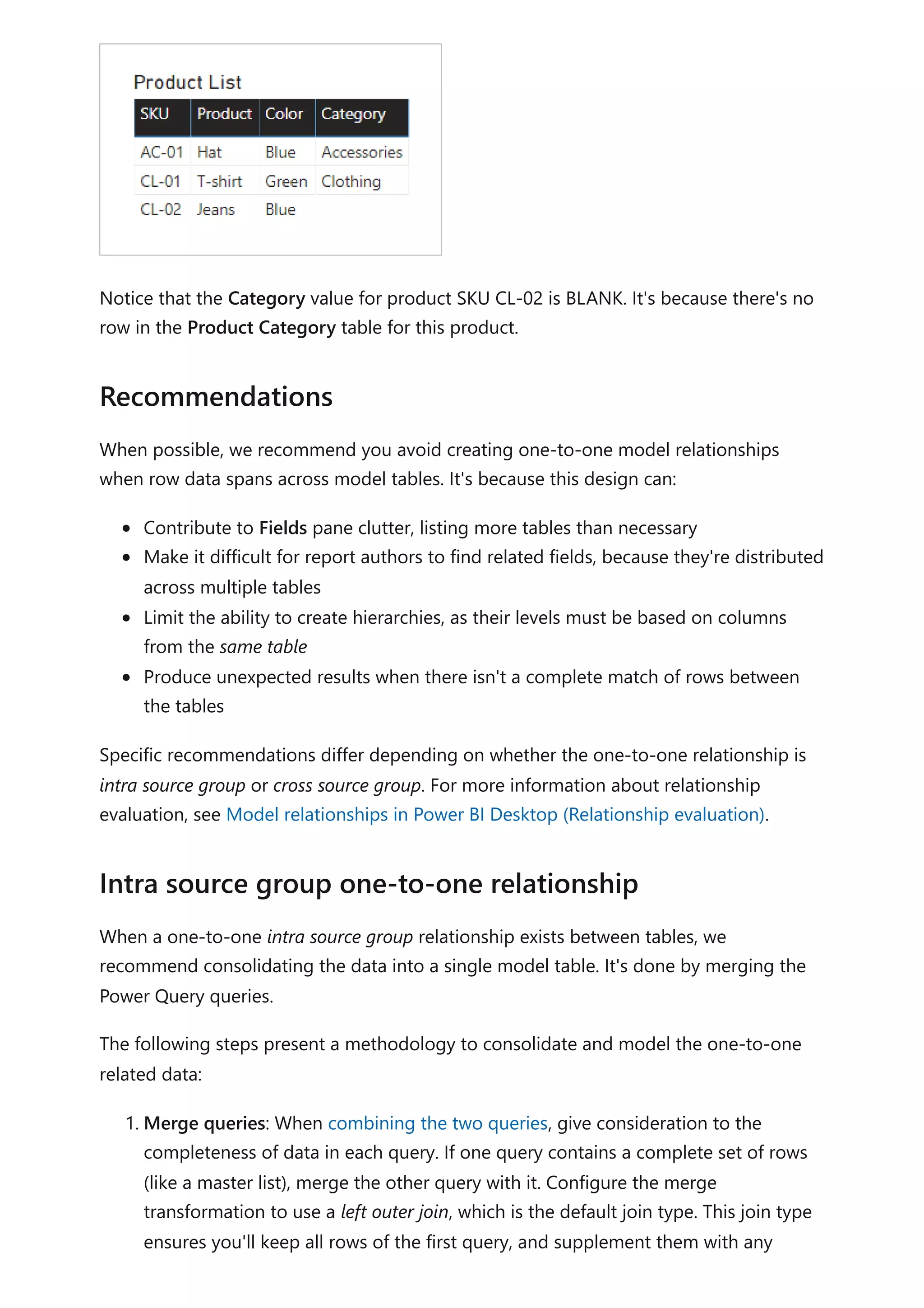
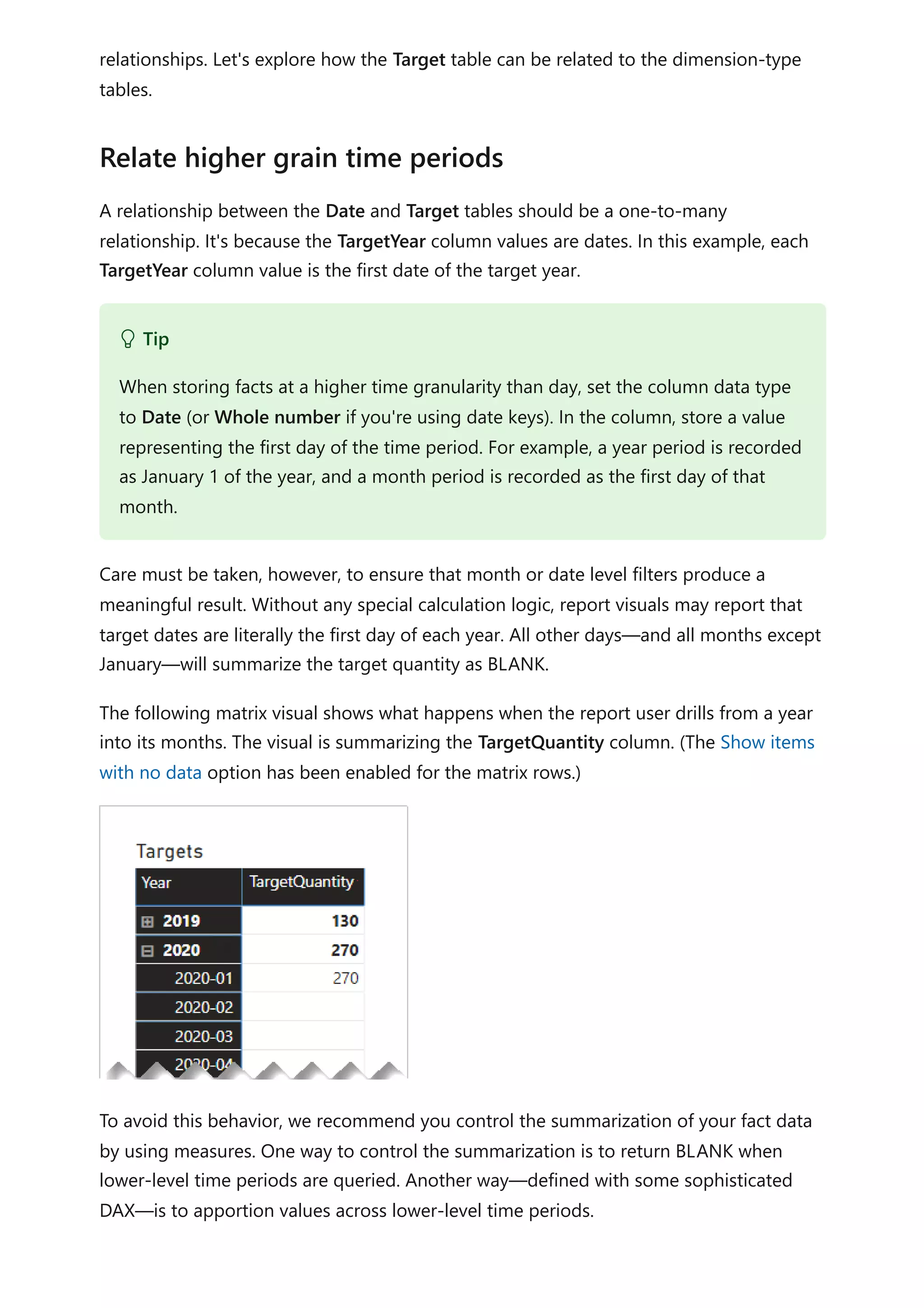
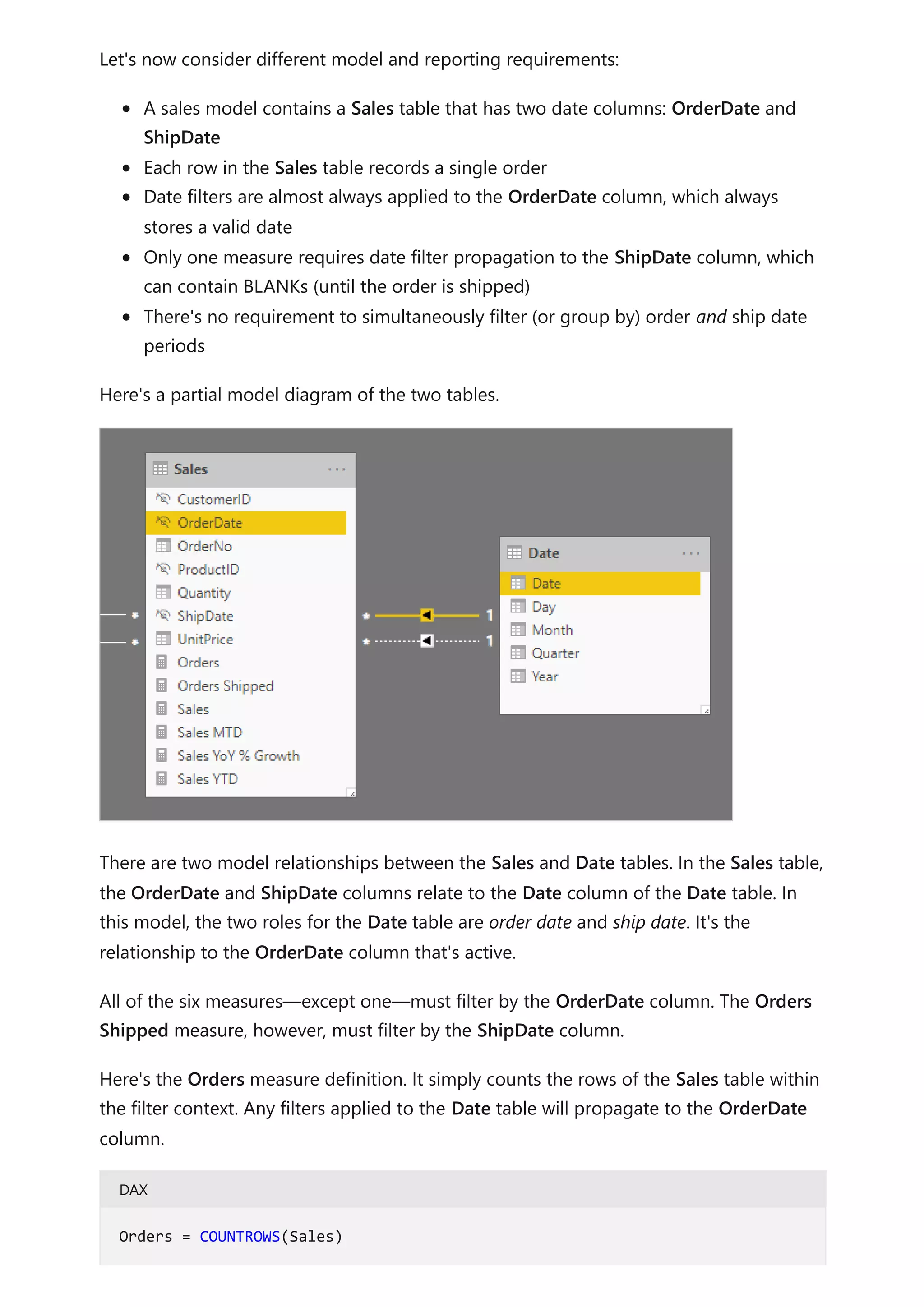
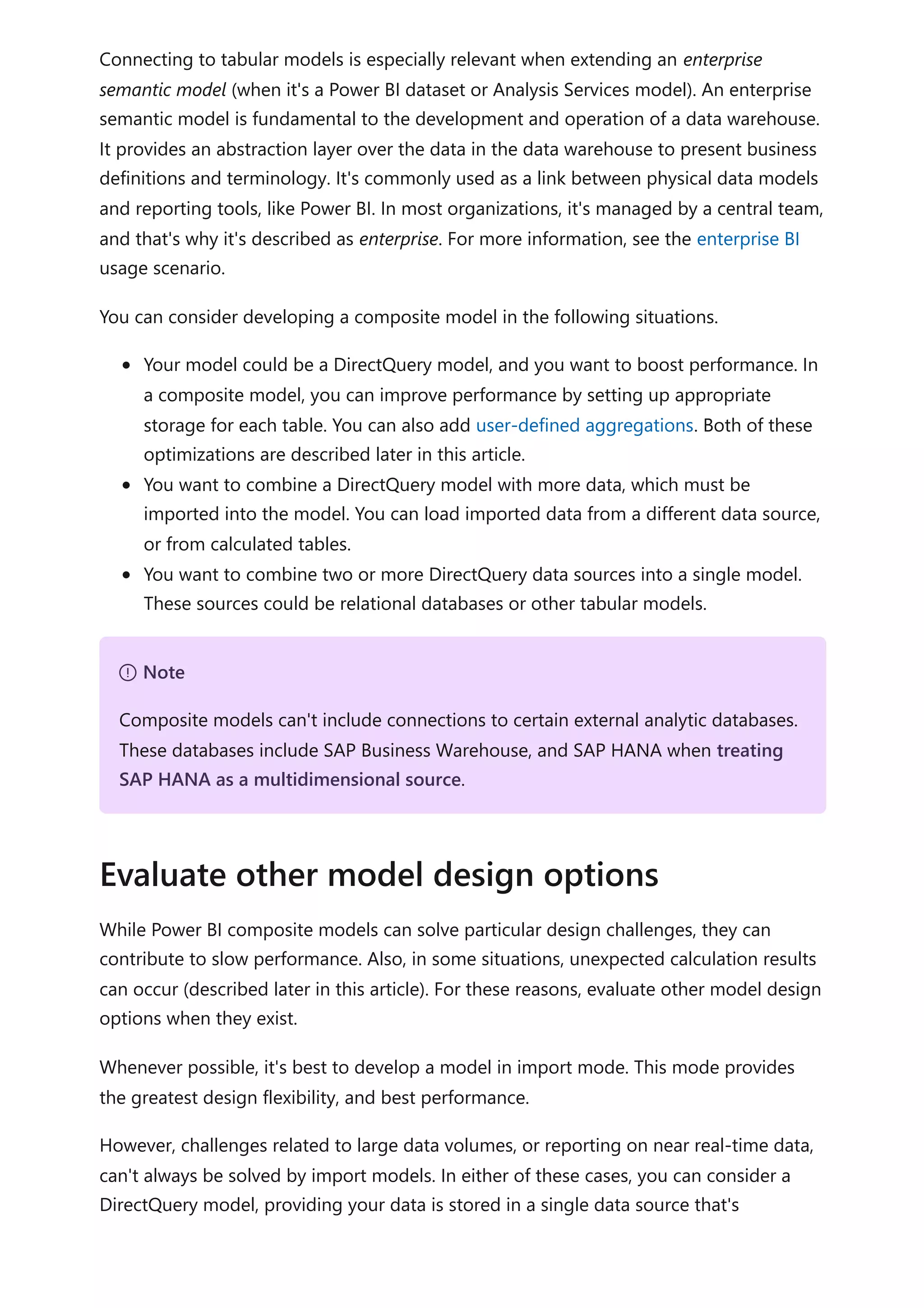
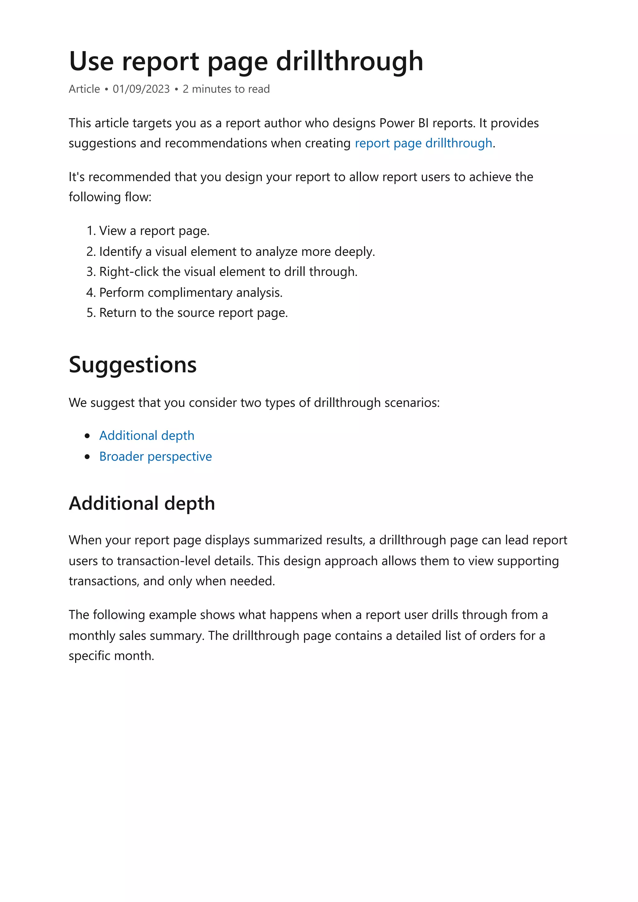
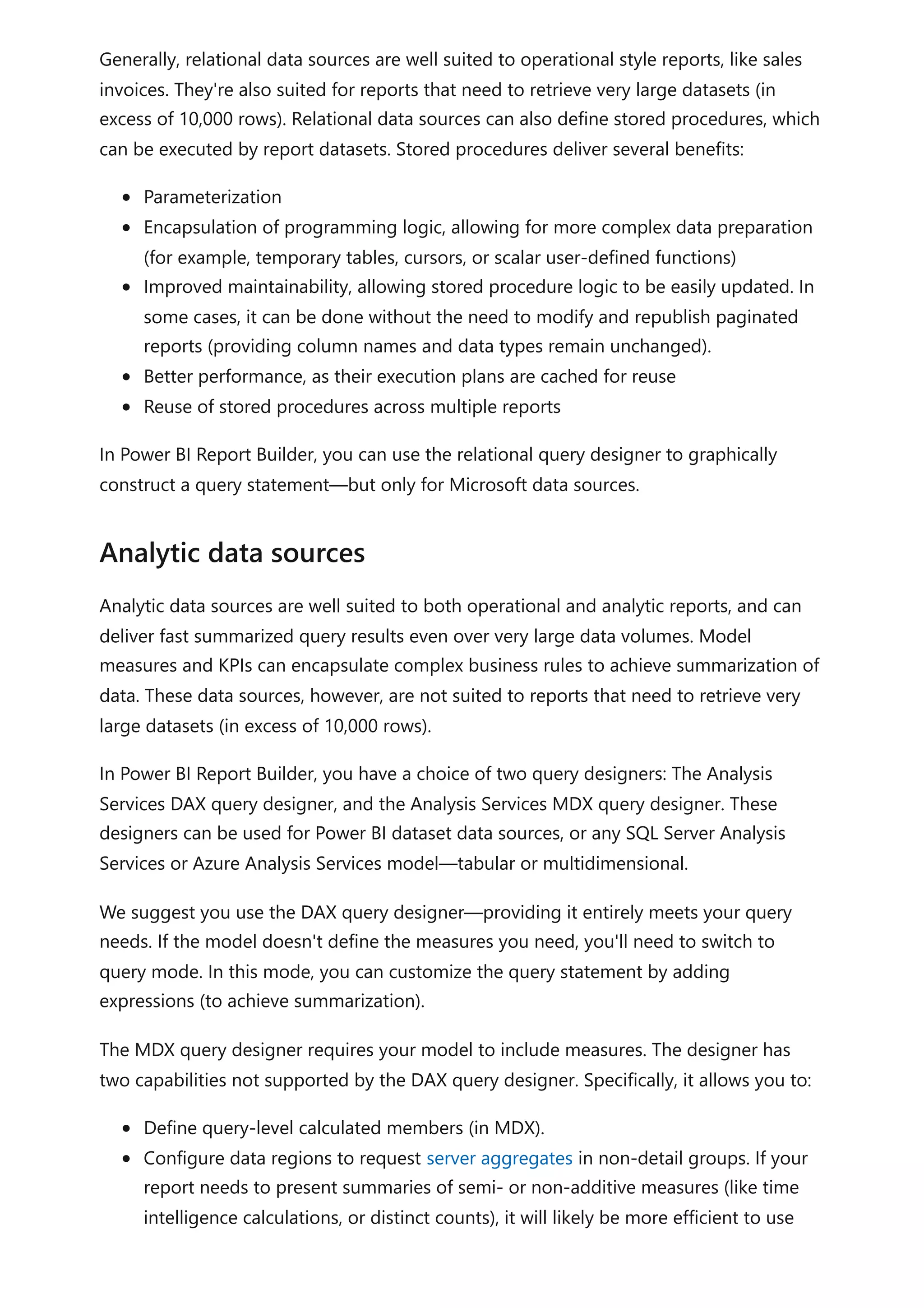
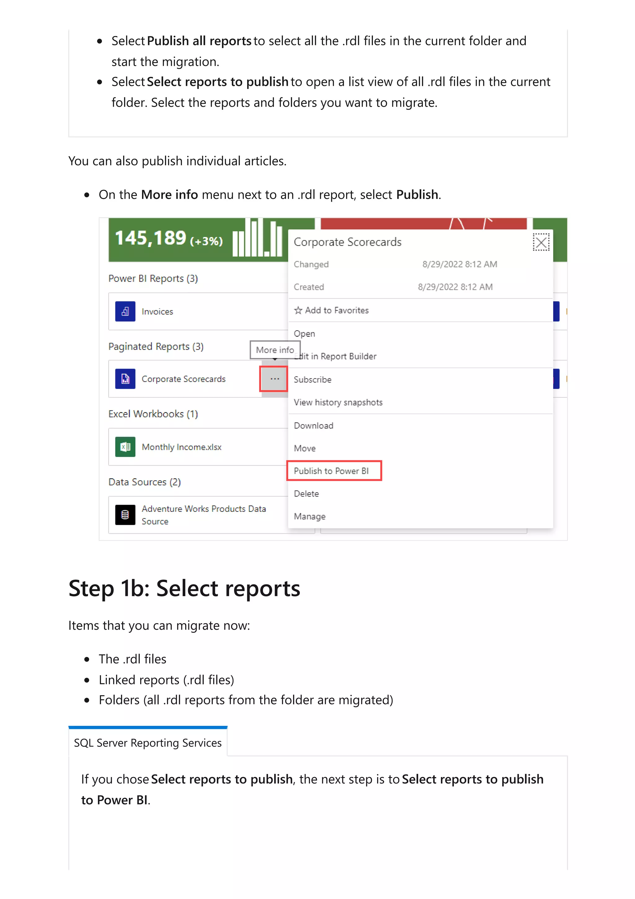
![This visual produces the correct result. Let's now consider what happens when the Color
column from the Product table is used to group target quantity.
The visual produces a misrepresentation of the data. What is happening here?
A filter on the Color column from the Product table results in two rows. One of the rows
is for the Clothing category, and the other is for the Accessories category. These two
category values are propagated as filters to the Target table. In other words, because
the color blue is used by products from two categories, those categories are used to
filter the targets.
To avoid this behavior, as described earlier, we recommend you control the
summarization of your fact data by using measures.
Consider the following measure definition. Notice that all Product table columns that
are beneath the category level are tested for filters.
DAX
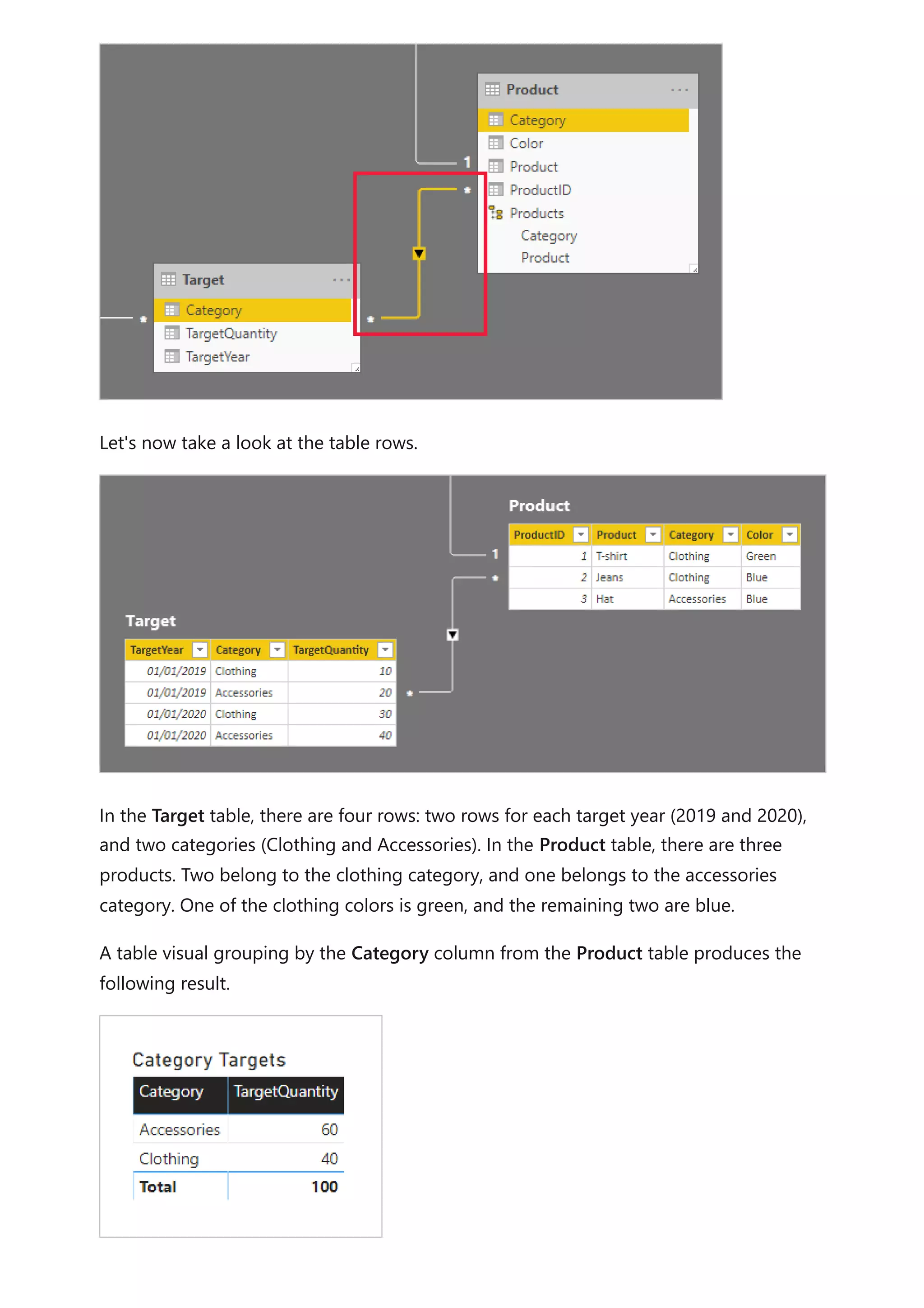
The following table visual now uses the Target Quantity measure. It shows that all color
target quantities are BLANK.
Target Quantity =
IF(
NOT ISFILTERED('Product'[ProductID])
&& NOT ISFILTERED('Product'[Product])
&& NOT ISFILTERED('Product'[Color]),
SUM(Target[TargetQuantity])
)](https://image.slidesharecdn.com/docpower-bi-guidance-230227102019-b6273799/75/DOC-Power-Bi-Guidance-pdf-70-2048.jpg)


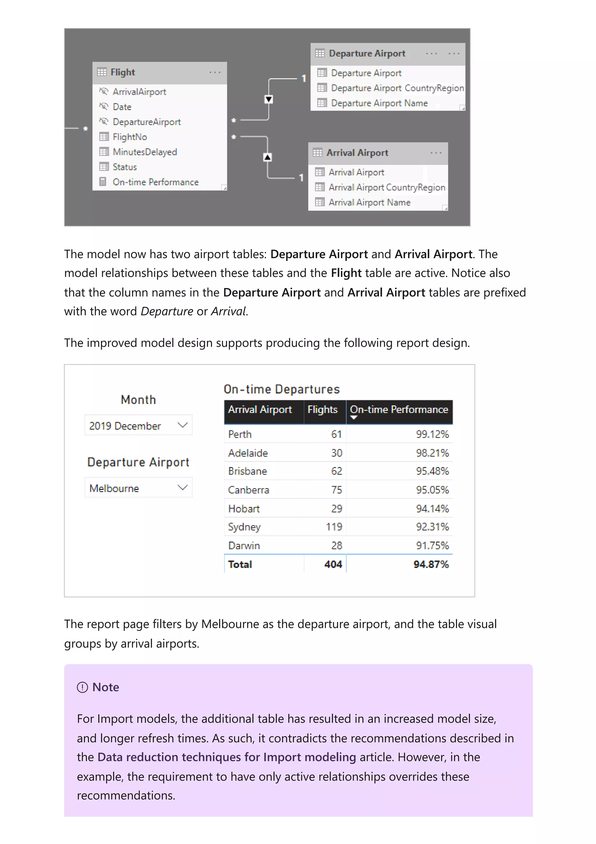
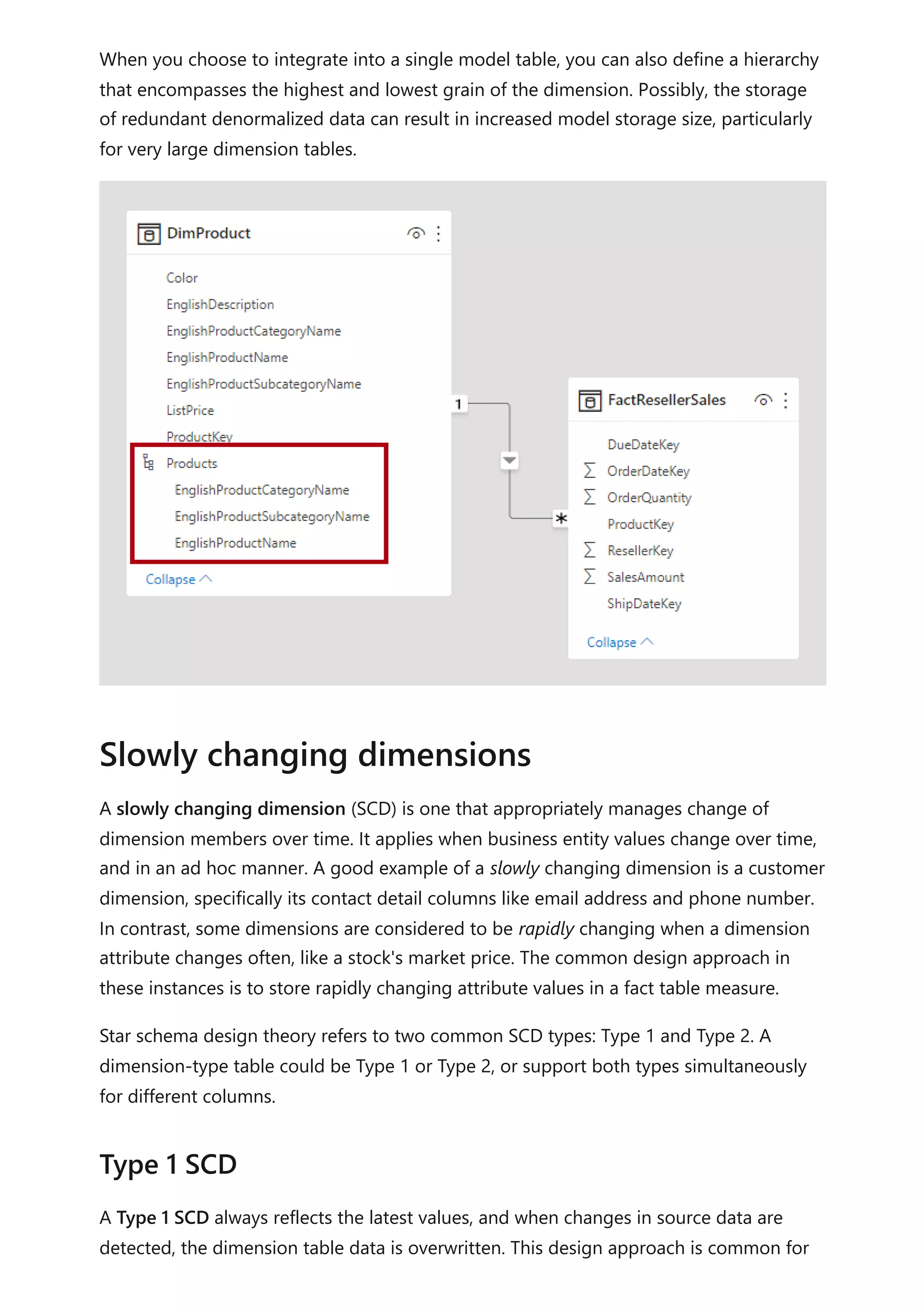
![Here's the Orders Shipped measure definition. It uses the USERELATIONSHIP DAX
function, which activates filter propagation for a specific relationship only during the
evaluation of the expression. In this example, the relationship to the ShipDate column is
used.
DAX
This model design supports producing the following report design.
The report page filters by quarter 2019 Q4. The table visual groups by month and
displays various sales statistics. The Orders and Orders Shipped measures produce
different results. They each use the same summarization logic (count rows of the Sales
table), but different Date table filter propagation.
Notice that the quarter slicer includes a BLANK item. This slicer item appears as a result
of table expansion. While each Sales table row has an order date, some rows have a
BLANK ship date—these orders are yet to be shipped. Table expansion considers
inactive relationships too, and so BLANKs can appear due to BLANKs on the many-side
of the relationship, or due to data integrity issues.
In summary, we recommend defining active relationships whenever possible. They
widen the scope and potential of how your model can be used by report authors, and
users working with Q&A. It means that role-playing dimension-type tables should be
duplicated in your model.
Orders Shipped =
CALCULATE(
COUNTROWS(Sales)
,USERELATIONSHIP('Date'[Date], Sales[ShipDate])
)
Recommendations](https://image.slidesharecdn.com/docpower-bi-guidance-230227102019-b6273799/75/DOC-Power-Bi-Guidance-pdf-78-2048.jpg)


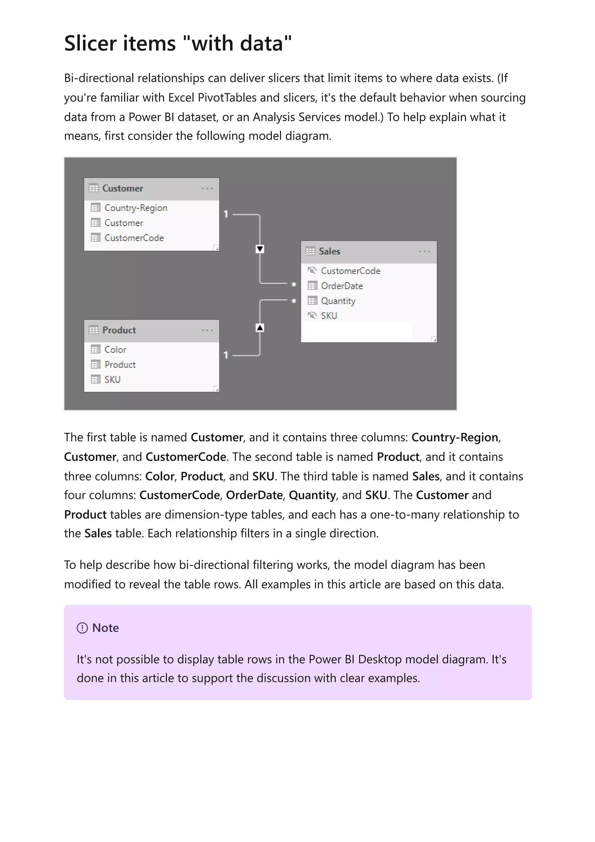
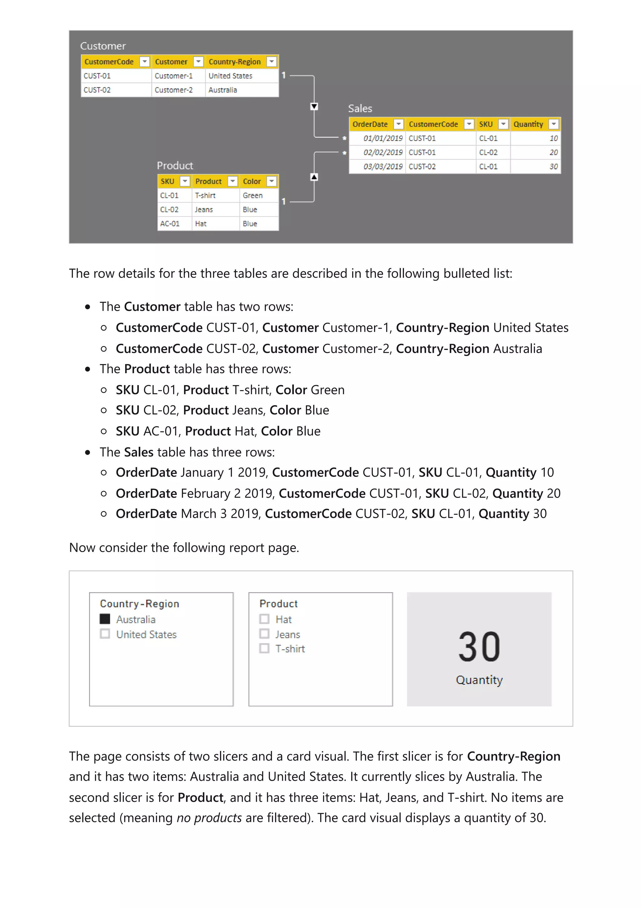
![Let's now consider that the relationship between the Product and Sales table no longer
filters in both directions. And, the following measure definition has been added to the
Sales table.
DAX
To show the Product slicer items "with data", it simply needs to be filtered by the Total
Quantity measure using the "is not blank" condition.
A different scenario involving bi-directional relationships treats a fact-type table like a
bridging table. This way, it supports analyzing dimension-type table data within the filter
context of a different dimension-type table.
Using the example model in this article, consider how the following questions can be
answered:
How many colors were sold to Australian customers?
How many countries/regions purchased jeans?
Both questions can be answered without summarizing data in the bridging fact-type
table. They do, however, require that filters propagate from one dimension-type table to
the other. Once filters propagate via the fact-type table, summarization of dimension-
type table columns can be achieved using the DISTINCTCOUNT DAX function—and
possibly the MIN and MAX DAX functions.
Total Quantity = SUM(Sales[Quantity])
Dimension-to-dimension analysis](https://image.slidesharecdn.com/docpower-bi-guidance-230227102019-b6273799/75/DOC-Power-Bi-Guidance-pdf-84-2048.jpg)
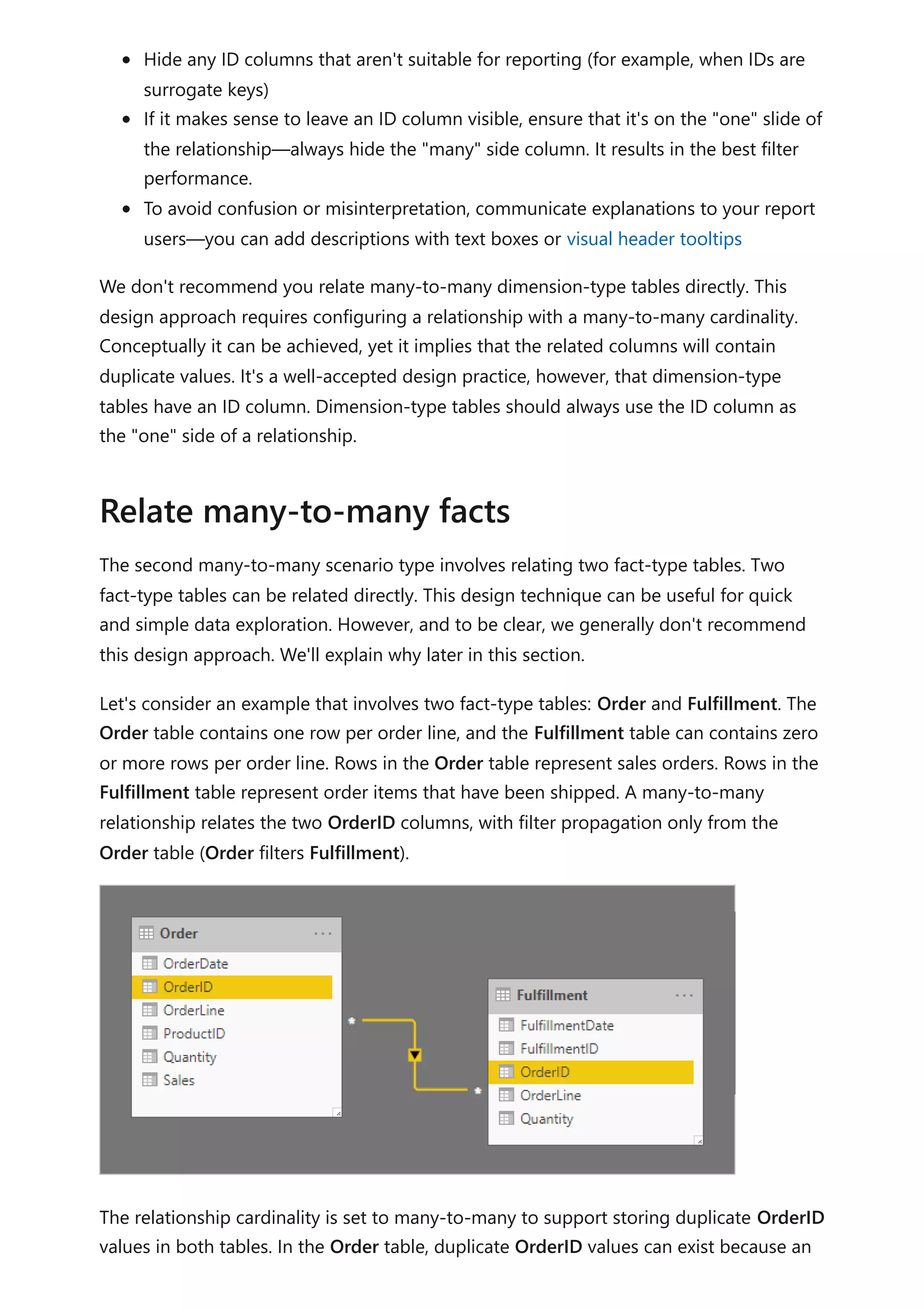
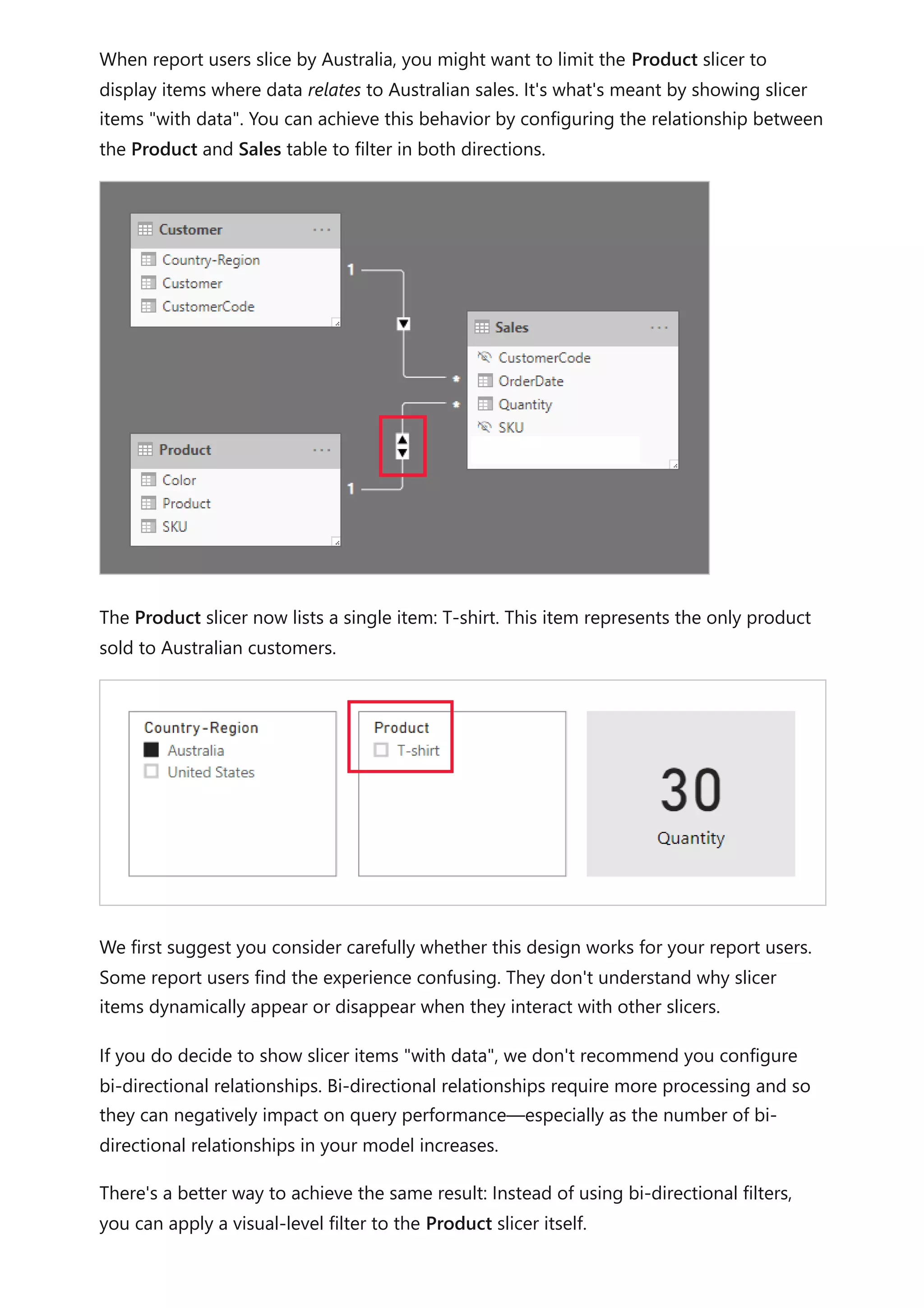
![As the fact-type table behaves like a bridging table, you can follow the many-to-many
relationship guidance to relate two dimension-type tables. It will require configuring at
least one relationship to filter in both directions. For more information, see Many-to-
many relationship guidance (Relate many-to-many dimensions).
However, as already described in this article, this design will likely result in a negative
impact on performance, and the user experience consequences related to slicer items
"with data". So, we recommend that you activate bi-directional filtering in a measure
definition by using the CROSSFILTER DAX function instead. The CROSSFILTER function
can be used to modify filter directions—or even disable the relationship—during the
evaluation of an expression.
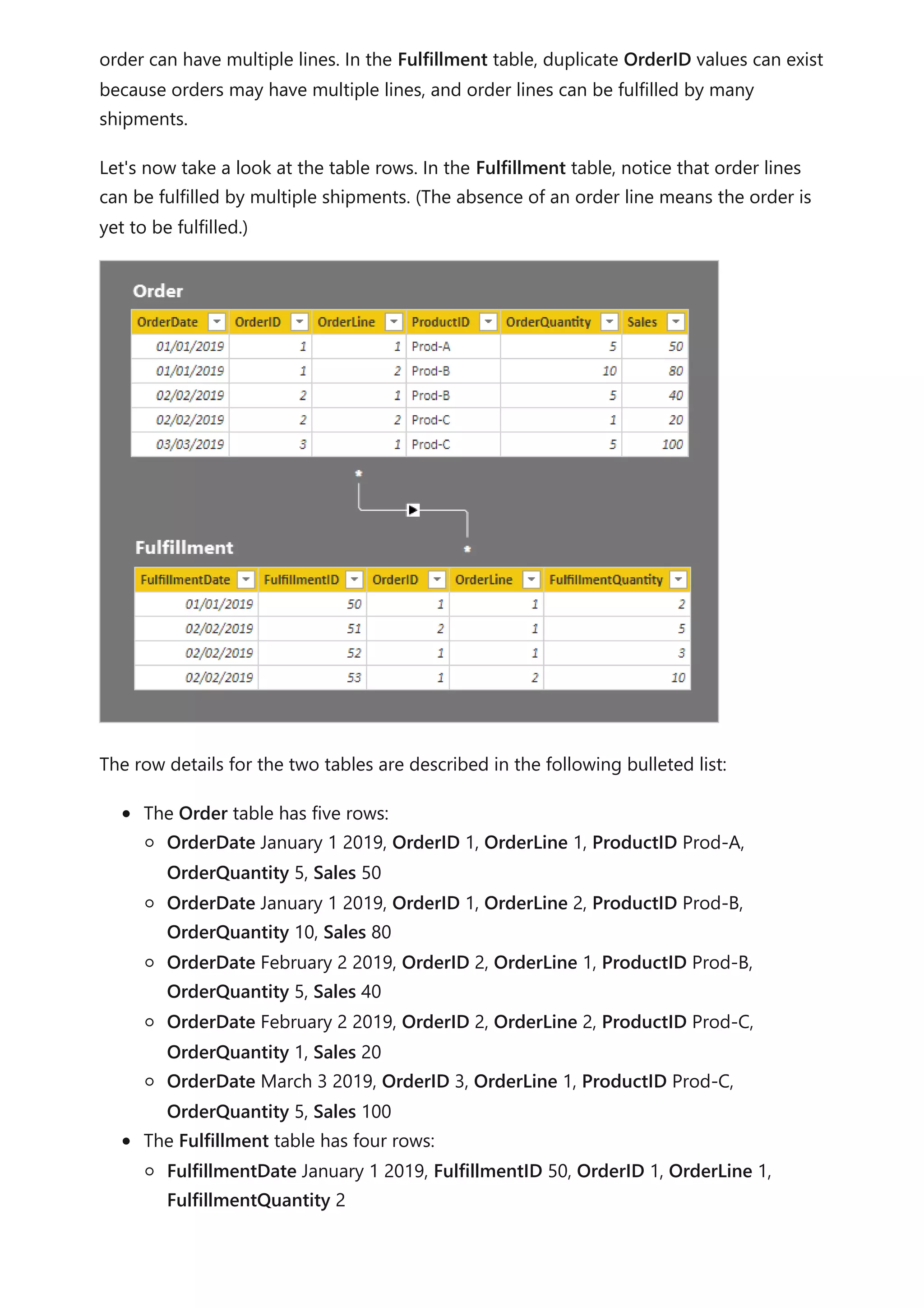
Consider the following measure definition added to the Sales table. In this example, the
model relationship between the Customer and Sales tables has been configured to filter
in a single direction.
DAX
During the evaluation of the Different Countries Sold measure expression, the
relationship between the Customer and Sales tables filters in both directions.
The following table visual present statistics for each product sold. The Quantity column
is simply the sum of quantity values. The Different Countries Sold column represents
the distinct count of country-region values of all customers who have purchased the
product.
Different Countries Sold =
CALCULATE(
DISTINCTCOUNT(Customer[Country-Region]),
CROSSFILTER(
Customer[CustomerCode],
Sales[CustomerCode],
BOTH
)
)](https://image.slidesharecdn.com/docpower-bi-guidance-230227102019-b6273799/75/DOC-Power-Bi-Guidance-pdf-85-2048.jpg)


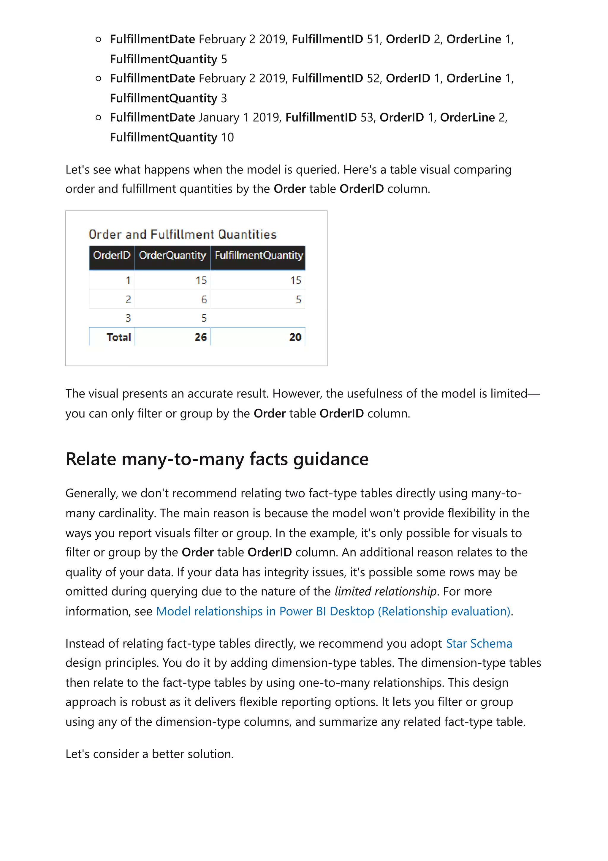
![Do not use Power Query relative date filtering: It's possible to define relative date
filtering in a Power Query query. For example, to retrieve to the sales orders that
were created in the last year (relative to today's date). This type of filter translates
to an inefficient native query, as follows:
SQL
A better design approach is to include relative time columns in the date table.
These columns store offset values relative to the current date. For example, in a
RelativeYear column, the value zero represents current year, -1 represents previous
year, etc. Preferably, the RelativeYear column is materialized in the date table.
While less efficient, it could also be added as a model calculated column, based on
the expression using the TODAY and DATE DAX functions.
Keep measures simple: At least initially, it's recommended to limit measures to
simple aggregates. The aggregate functions include SUM, COUNT, MIN, MAX, and
AVERAGE. Then, if the measures are sufficiently responsive, you can experiment
with more complex measures, but paying attention to the performance for each.
While the CALCULATE DAX function can be used to produce sophisticated measure
expressions that manipulate filter context, they can generate expensive native
queries that do not perform well.
Avoid relationships on calculated columns: Model relationships can only relate a
single column in one table to a single column in a different table. Sometimes,
however, it is necessary to relate tables by using multiple columns. For example,
the Sales and Geography tables are related by two columns: CountryRegion and
City. To create a relationship between the tables, a single column is required, and
in the Geography table, the column must contain unique values. Concatenating
the country/region and city with a hyphen separator could achieve this result.
The combined column can be created with either a Power Query custom column,
or in the model as a calculated column. However, it should be avoided as the
calculation expression will be embedded into the source queries. Not only is it
inefficient, it commonly prevents the use of indexes. Instead, add materialized
columns in the relational database source, and consider indexing them. You can
also consider adding surrogate key columns to dimension-type tables, which is a
common practice in relational data warehouse designs.
…
from [dbo].[Sales] as [_]
where [_].[OrderDate] >= convert(datetime2, '2018-01-01 00:00:00') and
[_].[OrderDate] < convert(datetime2, '2019-01-01 00:00:00'))](https://image.slidesharecdn.com/docpower-bi-guidance-230227102019-b6273799/75/DOC-Power-Bi-Guidance-pdf-94-2048.jpg)
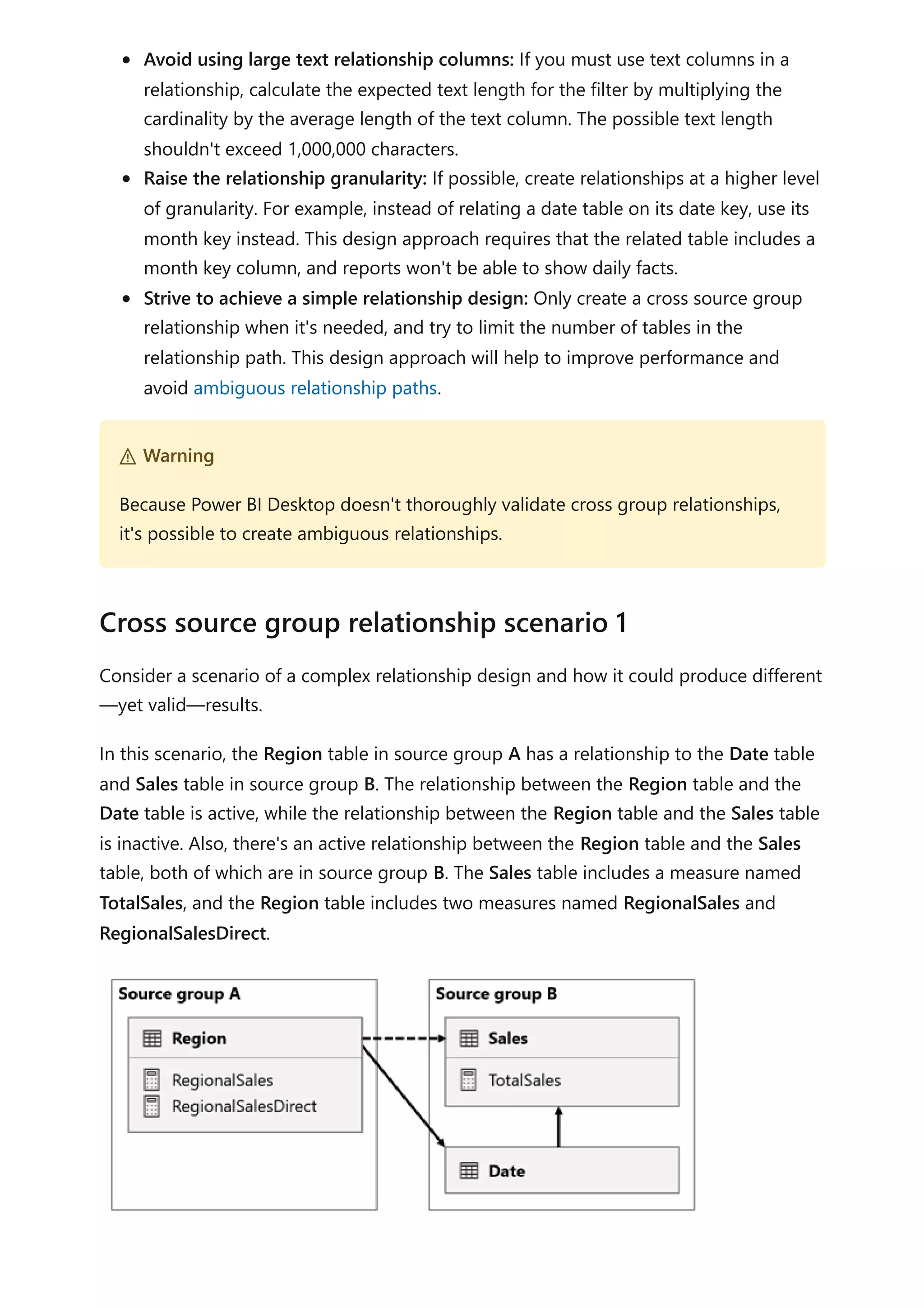
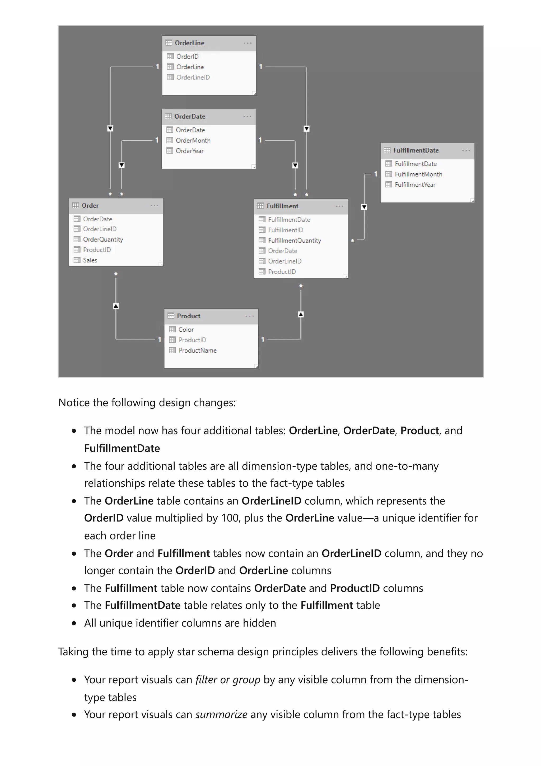
![Here are the measure definitions.
DAX
Notice how the RegionalSales measure refers to the TotalSales measure, while the
RegionalSalesDirect measure doesn't. Instead, the RegionalSalesDirect measure uses
the expression SUM(Sales[Sales]), which is the expression of the TotalSales measure.
The difference in the result is subtle. When Power BI evaluates the RegionalSales
measure, it applies the filter from the Region table to both the Sales table and the Date
table. Therefore, the filter also propagates from the Date table to the Sales table. In
contrast, when Power BI evaluates the RegionalSalesDirect measure, it only propagates
the filter from the Region table to the Sales table. The results returned by RegionalSales
measure and the RegionalSalesDirect measure could differ, even though the
expressions are semantically equivalent.
Consider a scenario when a cross source group relationship has high-cardinality
relationship columns.
In this scenario, the Date table is related to the Sales table on the DateKey columns. The
data type of the DateKey columns is integer, storing whole numbers that use the
yyyymmdd format. The tables belong to different source groups. Further, it's a high-
cardinality relationship because the earliest date in the Date table is January 1, 1900 and
the latest date is December 31, 2100—so there's a total of 73,414 rows in the table (one
row for each date in the 1900-2100 time span).
TotalSales = SUM(Sales[Sales])
RegionalSales = CALCULATE([TotalSales], USERELATIONSHIP(Region[RegionID],
Sales[RegionID]))
RegionalSalesDirect = CALCULATE(SUM(Sales[Sales]),
USERELATIONSHIP(Region[RegionID], Sales[RegionID]))
) Important
Whenever you use the CALCULATE function with an expression that's a measure in a
remote source group, test the calculation results thoroughly.
Cross source group relationship scenario 2](https://image.slidesharecdn.com/docpower-bi-guidance-230227102019-b6273799/75/DOC-Power-Bi-Guidance-pdf-108-2048.jpg)
![There are two cases for concern.
First, when you use the Date table columns as filters, filter propagation will filter the
DateKey column of the Sales table to evaluate measures. When filtering by a single year,
like 2022, the DAX query will include a filter expression like Sales[DateKey] IN {
20220101, 20220102, …20221231 }. The text size of the query can grow to become
extremely large when the number of values in the filter expression is large, or when the
filter values are long strings. It's expensive for Power BI to generate the long query and
for the data source to run the query.
Second, when you use Date table columns—like Year, Quarter, or Month—as grouping
columns, it results in filters that include all unique combinations of year, quarter, or
month, and the DateKey column values. The string size of the query, which contains
filters on the grouping columns and the relationship column, can become extremely
large. That's especially true when the number of grouping columns and/or the
cardinality of the join column (the DateKey column) is large.
To address any performance issues, you can:
Add the Date table to the data source, resulting in a single source group model
(meaning, it's no longer a composite model).
Raise the granularity of the relationship. For instance, you could add a MonthKey
column to both tables and create the relationship on those columns. However, by
raising the granularity of the relationship, you lose the ability to report on daily
sales activity (unless you use the DateKey column from the Sales table).
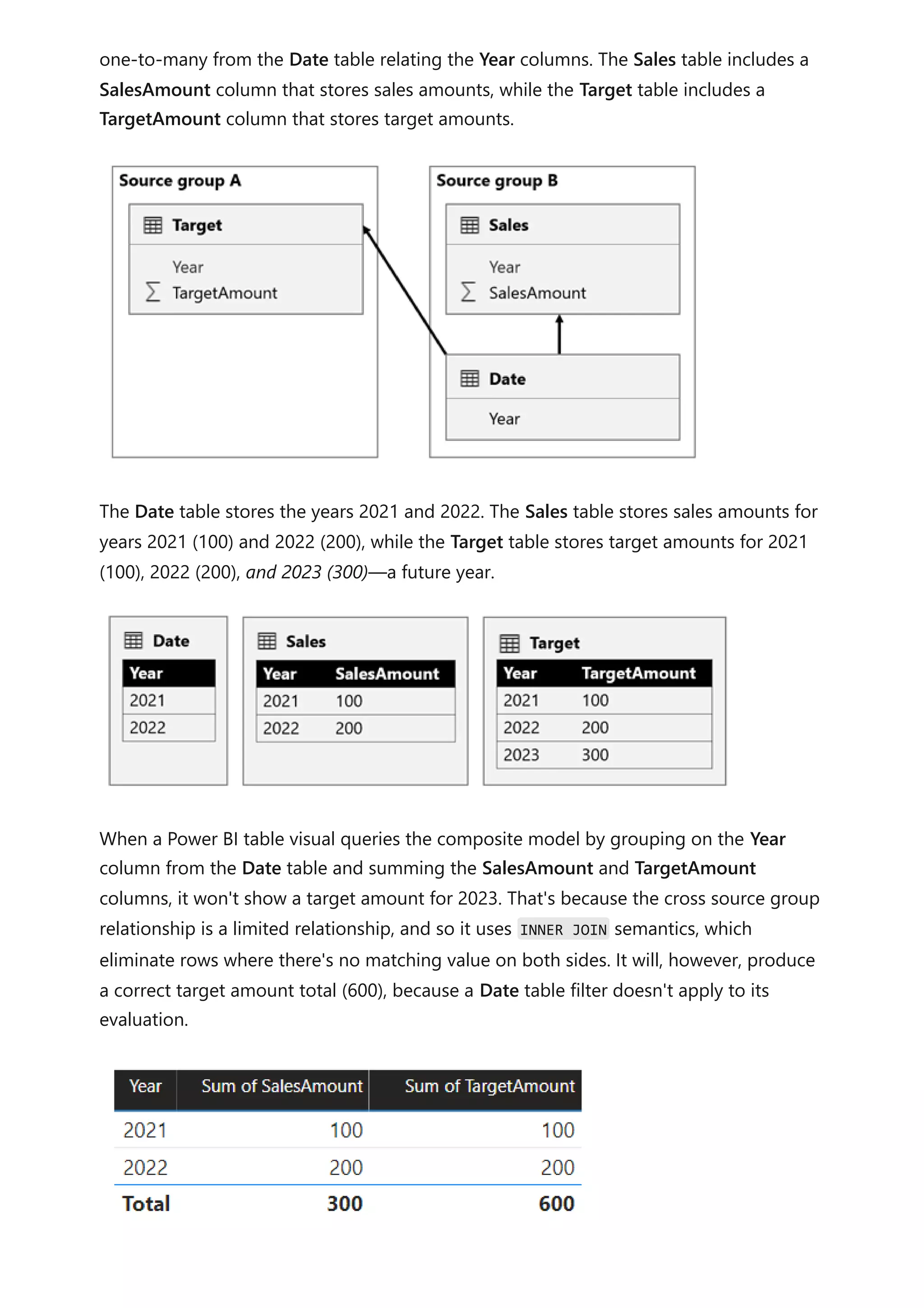
Consider a scenario when there aren't matching values between tables in a cross source
group relationship.
In this scenario, the Date table in source group B has a relationship to the Sales table in
that source group, and also to the Target table in source group A. All relationships are
Cross source group relationship scenario 3](https://image.slidesharecdn.com/docpower-bi-guidance-230227102019-b6273799/75/DOC-Power-Bi-Guidance-pdf-109-2048.jpg)
![If the relationship between the Date table and the Target table is an intra source group
relationship (assuming the Target table belonged to source group B), the visual will
include a (Blank) year to show the 2023 (and any other unmatched years) target amount.
For more information about limited relationships, see Relationship evaluation.
You should consider specific limitations when adding calculated columns and calculation
groups to a composite model.
Calculated columns added to a DirectQuery table that sources its data from a relational
database, like Microsoft SQL Server, are limited to expressions that operate on a single
row at a time. These expressions can't use DAX iterator functions, like SUMX, or filter
context modification functions, like CALCULATE.
A calculated column expression on a remote DirectQuery table is limited to intra-row
evaluation only. However, you can author such an expression, but it will result in an error
when it's used in a visual. For example, if you add a calculated column to a remote
DirectQuery table named DimProduct by using the expression [Product Sales] / SUM
(DimProduct[ProductSales]), you'll be able to successfully save the expression in the
model. However, it will result in an error when it's used in a visual because it violates the
intra-row evaluation restriction.
In contrast, calculated columns added to a remote DirectQuery table that's a tabular
model, which is either a Power BI dataset or Analysis Services model, are more flexible.
In this case, all DAX functions are allowed because the expression will be evaluated
within the source tabular model.
) Important
To avoid misreporting, ensure that there are matching values in the relationship
columns when dimension and fact tables reside in different source groups.
Calculations
Calculated columns
7 Note
It's not possible to added calculated columns or calculated tables that depend on
chained tabular models.](https://image.slidesharecdn.com/docpower-bi-guidance-230227102019-b6273799/75/DOC-Power-Bi-Guidance-pdf-111-2048.jpg)
![isn't enforced. Then, use the View As command on the Modeling ribbon tab to enforce
RLS and determine and compare query durations.
Once published to Power BI, you must map members to dataset roles. Only dataset
owners or workspace admins can add members to roles. For more information, see Row-
level security (RLS) with Power BI (Manage security on your model).
Members can be user accounts or security groups. Whenever possible, we recommend
you map security groups to dataset roles. It involves managing security group
memberships in Azure Active Directory. Possibly, it delegates the task to your network
administrators.
Test each role to ensure it filters the model correctly. It's easily done by using the View
As command on the Modeling ribbon tab.
When the model has dynamic rules using the USERNAME DAX function, be sure to test
for expected and unexpected values. When embedding Power BI content—specifically
using the embed for your customers scenario—app logic can pass any value as an
effective identity user name. Whenever possible, ensure accidental or malicious values
result in filters that return no rows.
Consider an example using Power BI embedded, where the app passes the user's job
role as the effective user name: It's either "Manager" or "Worker". Managers can see all
rows, but workers can only see rows where the Type column value is "Internal".
The following rule expression is defined:
DAX
The problem with this rule expression is that all values, except "Worker", return all table
rows. So, an accidental value, like "Wrker", unintentionally returns all table rows.
Therefore, it's safer to write an expression that tests for each expected value. In the
Configure role mappings
Validate roles
IF(
USERNAME() = "Worker",
[Type] = "Internal",
TRUE()
)](https://image.slidesharecdn.com/docpower-bi-guidance-230227102019-b6273799/75/DOC-Power-Bi-Guidance-pdf-118-2048.jpg)
![following improved rule expression, an unexpected value results in the table returning
no rows.
DAX
Sometimes, calculations need values that aren't constrained by RLS filters. For example,
a report may need to display a ratio of revenue earned for the report user's sales region
over all revenue earned.
While it's not possible for a DAX expression to override RLS—in fact, it can't even
determine that RLS is enforced—you can use a summary model table. The summary
model table is queried to retrieve revenue for "all regions" and it's not constrained by
any RLS filters.
Let's see how you could implement this design requirement. First, consider the following
model design:
The model comprises four tables:
IF(
USERNAME() = "Worker",
[Type] = "Internal",
IF(
USERNAME() = "Manager",
TRUE(),
FALSE()
)
)
Design partial RLS](https://image.slidesharecdn.com/docpower-bi-guidance-230227102019-b6273799/75/DOC-Power-Bi-Guidance-pdf-119-2048.jpg)
![The Salesperson table stores one row per salesperson. It includes the
EmailAddress column, which stores the email address for each salesperson. This
table is hidden.
The Sales table stores one row per order. It includes the Revenue % All Region
measure, which is designed to return a ratio of revenue earned by the report user's
region over revenue earned by all regions.
The Date table stores one row per date and allows filtering and grouping year and
month.
The SalesRevenueSummary is a calculated table. It stores total revenue for each
order date. This table is hidden.
The following expression defines the SalesRevenueSummary calculated table:
DAX
The following RLS rule is applied to the Salesperson table:
DAX
Each of the three model relationships is described in the following table:
Relationship Description
There's a many-to-many relationship between the Salesperson and Sales tables.
The RLS rule filters the EmailAddress column of the hidden Salesperson table by
using the USERNAME DAX function. The Region column value (for the report user)
propagates to the Sales table.
There's a one-to-many relationship between the Date and Sales tables.
There's a one-to-many relationship between the Date and
SalesRevenueSummary tables.
SalesRevenueSummary =
SUMMARIZECOLUMNS(
Sales[OrderDate],
"RevenueAllRegion", SUM(Sales[Revenue])
)
7 Note
An aggregation table could achieve the same design requirement.
[EmailAddress] = USERNAME()](https://image.slidesharecdn.com/docpower-bi-guidance-230227102019-b6273799/75/DOC-Power-Bi-Guidance-pdf-120-2048.jpg)
![The following expression defines the Revenue % All Region measure:
DAX
Sometimes it makes sense to avoid using RLS. If you have only a few simplistic RLS rules
that apply static filters, consider publishing multiple datasets instead. None of the
datasets define roles because each dataset contains data for a specific report user
audience, which has the same data permissions. Then, create one workspace per
audience and assign access permissions to the workspace or app.
For example, a company that has just two sales regions decides to publish a dataset for
each sales region to different workspaces. The datasets don't enforce RLS. They do,
however, use query parameters to filter source data. This way, the same model is
published to each workspace—they just have different dataset parameter values.
Salespeople are assigned access to just one of the workspaces (or published apps).
There are several advantages associated with avoiding RLS:
Improved query performance: It can result in improved performance due to fewer
filters.
Smaller models: While it results in more models, they're smaller in size. Smaller
models can improve query and data refresh responsiveness, especially if the
hosting capacity experiences pressure on resources. Also, it's easier to keep model
sizes below size limits imposed by your capacity. Lastly, it's easier to balance
workloads across different capacities, because you can create workspaces on—or
move workspaces to—different capacities.
Additional features: Power BI features that don't work with RLS, like Publish to
web, can be used.
Revenue % All Region =
DIVIDE(
SUM(Sales[Revenue]),
SUM(SalesRevenueSummary[RevenueAllRegion])
)
7 Note
Take care to avoid disclosing sensitive facts. If there are only two regions in this
example, then it would be possible for a report user to calculate revenue for the
other region.
When to avoid using RLS](https://image.slidesharecdn.com/docpower-bi-guidance-230227102019-b6273799/75/DOC-Power-Bi-Guidance-pdf-121-2048.jpg)
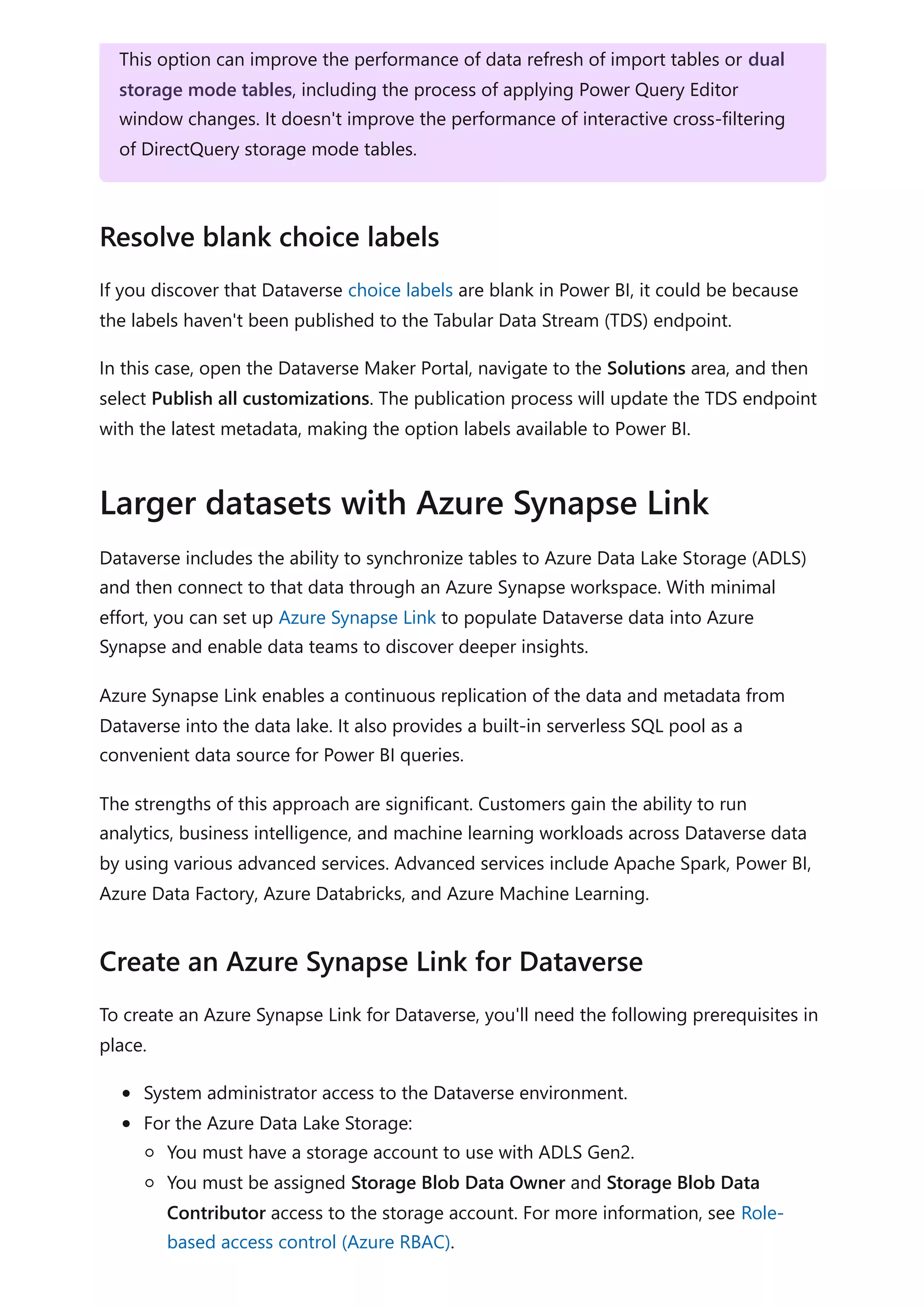
![By default, when you use Power Query to load a Dataverse table, it retrieves all rows and
all columns. When you query a system user table, for example, it could contain more
than 1,000 columns. The columns in the metadata include relationships to other entities
and lookups to option labels, so the total number of columns grows with the complexity
of the Dataverse table.
Attempting to retrieve data from all columns is an anti-pattern. It often results in
extended data refresh operations, and it will cause the query to fail when the data
volume exceeds 80 MB.
We recommend that you only retrieve columns that are required by reports. It's often a
good idea to reevaluate and refactor queries when report development is complete,
allowing you to identify and remove unused columns. For more information, see Data
reduction techniques for import modeling (Remove unnecessary columns).
Additionally, ensure that you introduce the Power Query Remove columns step early so
that it folds back to the source. That way, Power Query can avoid the unnecessary work
of extracting source data only to discard it later (in an unfolded step).
When you have a table that contains many columns, it might be impractical to use the
Power Query interactive query builder. In this case, you can start by creating a blank
query. You can then use the Advanced Editor to paste in a minimal query that creates a
starting point.
Consider the following query that retrieves data from just two columns of the account
table.
Power Query M
7 Note
Optimizing Power Query is a broad topic. To achieve a better understanding of
what Power Query is doing at authoring and at model refresh time in Power BI
Desktop, see Query diagnostics.
Minimize the number of query columns
let
Source = CommonDataService.Database("demo.crm.dynamics.com",
[CreateNavigationProperties=false]),
dbo_account = Source{[Schema="dbo", Item="account"]}[Data],
#"Removed Other Columns" = Table.SelectColumns(dbo_account,
{"accountid", "name"})](https://image.slidesharecdn.com/docpower-bi-guidance-230227102019-b6273799/75/DOC-Power-Bi-Guidance-pdf-130-2048.jpg)
![When you have specific transformation requirements, you might achieve better
performance by using a native query written in Dataverse SQL, which is a subset of
Transact-SQL. You can write a native query to:
Reduce the number of rows (by using a WHERE clause).
Aggregate data (by using the GROUP BY and HAVING clauses).
Join tables in a specific way (by using the JOIN or APPLY syntax).
Use supported SQL functions.
For more information, see:
Use SQL to query data
How Dataverse SQL differs from Transact-SQL
Power Query executes a native query by using the Value.NativeQuery function.
When using this function, it's important to add the EnableFolding=true option to ensure
queries are folded back to the Dataverse service. A native query won't fold unless this
option is added. Enabling this option can result in significant performance
improvements—up to 97 percent faster in some cases.
Consider the following query that uses a native query to source selected columns from
the account table. The native query will fold because the EnableFolding=true option is
set.
Power Query M
in
#"Removed Other Columns"
Write native queries
Execute native queries with the EnableFolding option
let
Source = CommonDataService.Database("demo.crm.dynamics.com"),
dbo_account = Value.NativeQuery(
Source,
"SELECT A.accountid, A.name FROM account A"
,null
,[EnableFolding=true]
)
in
dbo_account](https://image.slidesharecdn.com/docpower-bi-guidance-230227102019-b6273799/75/DOC-Power-Bi-Guidance-pdf-131-2048.jpg)
![When you set the CreateNavigationProperties=false option, the territoryid and
territoryidname columns will remain, but the territory column, which is a relationship
column (it shows Value links), will be excluded. It's important to understand that Power
Query relationship columns are a different concept to model relationships, which
propagate filters between model tables.
Consider the following query that uses the CreateNavigationProperties=false option (in
the Source step) to speed up the evaluation stage of a data import.
Power Query M
When using this option, you're likely to experience significant performance
improvement when a Dataverse table has many relationships to other tables. For
example, because the SystemUser table is related to every other table in the database,
refresh performance of this table would benefit by setting the
CreateNavigationProperties=false option.
let
Source = CommonDataService.Database("demo.crm.dynamics.com"
,[CreateNavigationProperties=false]),
dbo_account = Source{[Schema="dbo", Item="account"]}[Data],
#"Removed Other Columns" = Table.SelectColumns(dbo_account,
{"accountid", "name", "address1_stateorprovince", "address1_country",
"industrycodename", "territoryidname"}),
#"Renamed Columns" = Table.RenameColumns(#"Removed Other Columns",
{{"name", "Account Name"}, {"address1_country", "Country"},
{"address1_stateorprovince", "State or Province"}, {"territoryidname",
"Territory"}, {"industrycodename", "Industry"}})
in
#"Renamed Columns"
7 Note](https://image.slidesharecdn.com/docpower-bi-guidance-230227102019-b6273799/75/DOC-Power-Bi-Guidance-pdf-133-2048.jpg)
![This approach delivers data to Power BI that's focused, enriched, and filtered.
You can create a serverless SQL pool in the Azure Synapse workspace by using Azure
Synapse Studio. Select Serverless as the SQL pool type and enter a database name.
Power Query can connect to this pool by connecting to the workspace SQL endpoint.
You can create custom views that wrap serverless SQL pool queries. These views will
serve as straightforward, clean sources of data that Power BI connects to. The views
should:
Include the labels associated with choice fields.
Reduce complexity by including only the columns required for data modeling.
Filter out unnecessary rows, such as inactive records.
Consider the following view that retrieves campaign data.
SQL
Create custom views
CREATE VIEW [VW_Campaign]
AS
SELECT
[base].[campaignid] AS [CampaignID]
[base].[name] AS [Campaign],
[campaign_status].[LocalizedLabel] AS [Status],
[campaign_typecode].[LocalizedLabel] AS [Type Code]
FROM
[<MySynapseLinkDB>].[dbo].[campaign] AS [base]
LEFT OUTER JOIN [<MySynapseLinkDB>].[dbo].[OptionsetMetadata] AS
[campaign_typecode]
ON [base].[typecode] = [campaign_typecode].[option]
AND [campaign_typecode].[LocalizedLabelLanguageCode] = 1033
AND [campaign_typecode].[EntityName] = 'campaign'
AND [campaign_typecode].[OptionSetName] = 'typecode'
LEFT OUTER JOIN [<MySynapseLinkDB>].[dbo].[StatusMetadata] AS
[campaign_status]
ON [base].[statuscode] = [campaign_Status].[status]](https://image.slidesharecdn.com/docpower-bi-guidance-230227102019-b6273799/75/DOC-Power-Bi-Guidance-pdf-136-2048.jpg)
![Notice that the view includes only four columns, each aliased with a friendly name.
There's also a WHERE clause to return only necessary rows, in this case active campaigns.
Also, the view queries the campaign table that's joined to the OptionsetMetadata and
StatusMetadata tables, which retrieve choice labels.
Azure Synapse Link for Dataverse ensures that data is continually synchronized with the
data in the data lake. For high-usage activity, simultaneous writes and reads can create
locks that cause queries to fail. To ensure reliability when retrieving data, two versions of
the table data are synchronized in Azure Synapse.
Near real-time data: Provides a copy of data synchronized from Dataverse via
Azure Synapse Link in an efficient manner by detecting what data has changed
since it was initially extracted or last synchronized.
Snapshot data: Provides a read-only copy of near real-time data that's updated at
regular intervals (in this case every hour). Snapshot data table names have
_partitioned appended to their name.
If you anticipate that a high volume of read and write operations will be executed
simultaneously, retrieve data from the snapshot tables to avoid query failures.
For more information, see Access near real-time data and read-only snapshot data.
To query an Azure Synapse serverless SQL pool, you'll need its workspace SQL endpoint.
You can retrieve the endpoint from Synapse Studio by opening the serverless SQL pool
properties.
In Power BI Desktop, you can connect to Azure Synapse by using the Azure Synapse
Analytics SQL connector. When prompted for the server, enter the workspace SQL
AND [campaign_status].[LocalizedLabelLanguageCode] = 1033
AND [campaign_status].[EntityName] = 'campaign'
WHERE
[base].[statecode] = 0;
Tip
For more information on how to retrieve metadata, see Access choice labels
directly from Azure Synapse Link for Dataverse.
Query appropriate tables
Connect to Synapse Analytics](https://image.slidesharecdn.com/docpower-bi-guidance-230227102019-b6273799/75/DOC-Power-Bi-Guidance-pdf-137-2048.jpg)
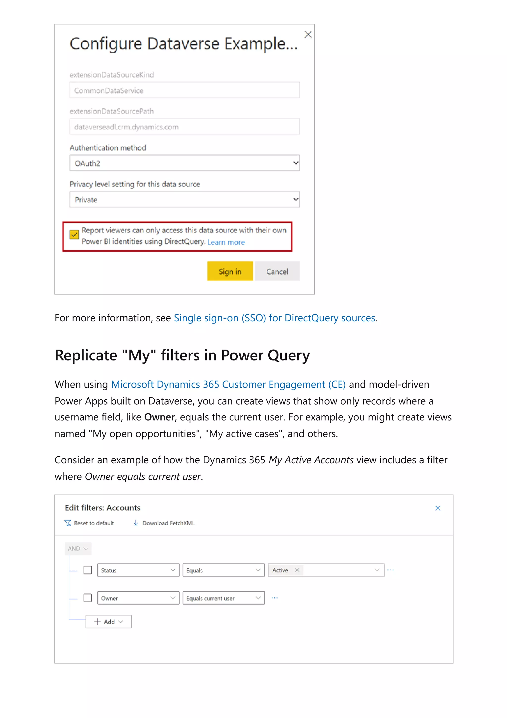
![You can reproduce this result in Power Query by using a native query that embeds the
CURRENT_USER token.
Consider the following example that shows a native query that returns the accounts for
the current user. In the WHERE clause, notice that the ownerid column is filtered by the
CURRENT_USER token.
Power Query M
When you publish the model to the Power BI service, you must enable single sign-on
(SSO) so that Power BI will send the report user's authenticated Azure AD credentials to
Dataverse.
You can create a DirectQuery model that enforces Dataverse permissions knowing that
performance will be slow. You can then supplement this model with import models that
target specific subjects or audiences that could enforce RLS permissions.
For example, an import model could provide access to all Dataverse data but not
enforce any permissions. This model would be suited to executives who already have
access to all Dataverse data.
As another example, when Dataverse enforces role-based permissions by sales region,
you could create one import model and replicate those permissions using RLS.
Alternatively, you could create a model for each sales region. You could then grant read
permission to those models (datasets) to the salespeople of each region. To facilitate the
creation of these regional models, you can use parameters and report templates. For
more information, see Create and use report templates in Power BI Desktop.
let
Source = CommonDataService.Database("demo.crm.dynamics.com",
[CreateNavigationProperties=false],
dbo_account = Value.NativeQuery(Source, "
SELECT
accountid, accountnumber, ownerid, address1_city,
address1_stateorprovince, address1_country
FROM account
WHERE statecode = 0
AND ownerid = CURRENT_USER
", null, [EnableFolding]=true])
in
dbo_account
Create supplementary import models](https://image.slidesharecdn.com/docpower-bi-guidance-230227102019-b6273799/75/DOC-Power-Bi-Guidance-pdf-141-2048.jpg)

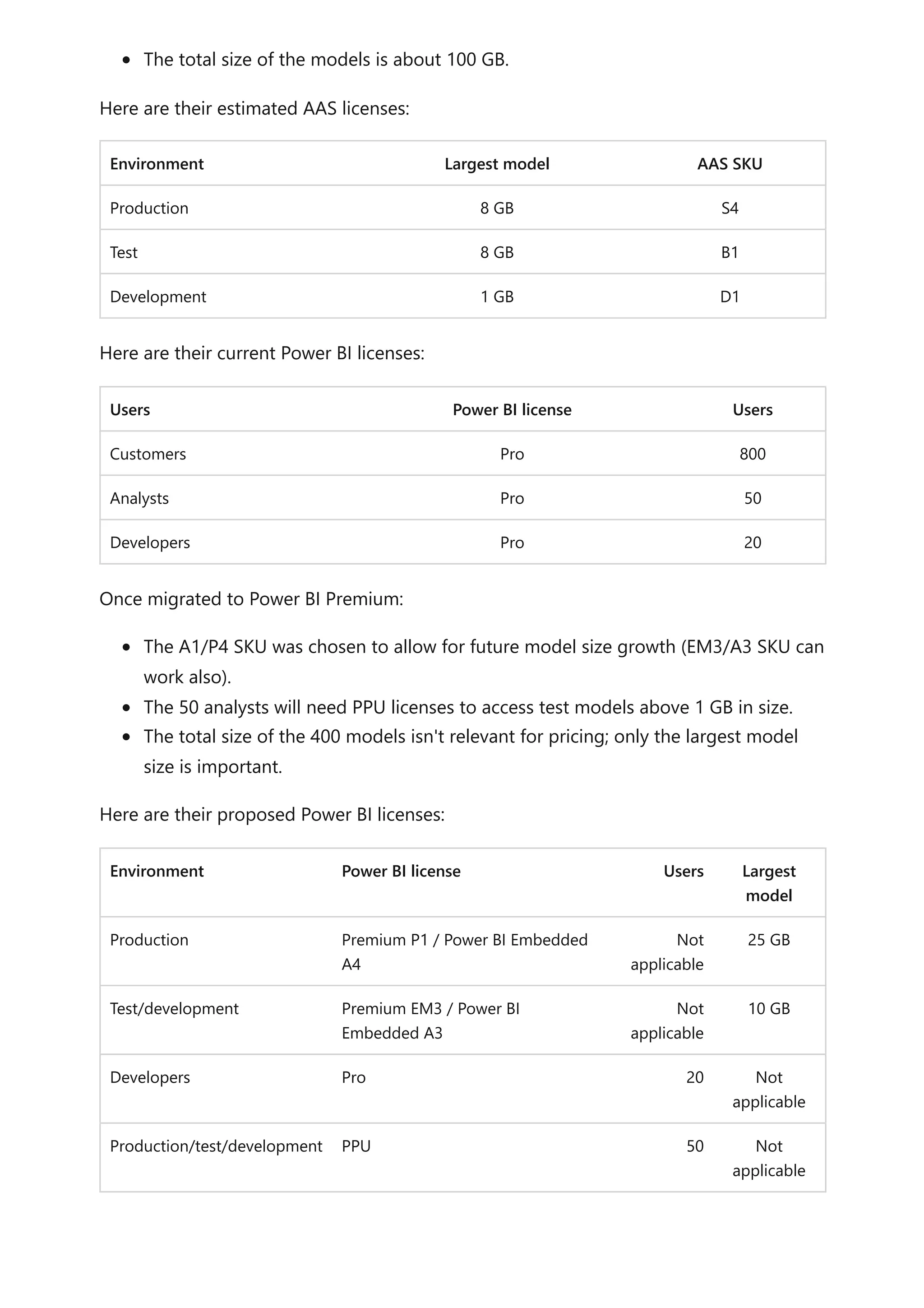
![be returned instead. The DIVIDE function is one such example. For additional
guidance about this function, read the DAX: DIVIDE function vs divide operator (/)
article.
The following measure expression tests whether an error would be raised. It returns
BLANK in this instance (which is the case when you do not provide the IF function with a
value-if-false expression).
DAX
This next version of the measure expression has been improved by using the IFERROR
function in place of the IF and ISERROR functions.
DAX
However, this final version of the measure expression achieves the same outcome, yet
more efficiently and elegantly.
DAX
Learning path: Use DAX in Power BI Desktop
Questions? Try asking the Power BI Community
Suggestions? Contribute ideas to improve Power BI
Example
Profit Margin
= IF(ISERROR([Profit] / [Sales]))
Profit Margin
= IFERROR([Profit] / [Sales], BLANK())
Profit Margin
= DIVIDE([Profit], [Sales])
See also](https://image.slidesharecdn.com/docpower-bi-guidance-230227102019-b6273799/75/DOC-Power-Bi-Guidance-pdf-165-2048.jpg)
![Avoid converting BLANKs to values
Article • 09/20/2022 • 2 minutes to read
As a data modeler, when writing measure expressions you might come across cases
where a meaningful value can't be returned. In these instances, you may be tempted to
return a value—like zero—instead. It's suggested you carefully determine whether this
design is efficient and practical.
Consider the following measure definition that explicitly converts BLANK results to zero.
DAX
Consider another measure definition that also converts BLANK results to zero.
DAX
The DIVIDE function divides the Profit measure by the Sales measure. Should the result
be zero or BLANK, the third argument—the alternate result (which is optional)—is
returned. In this example, because zero is passed as the alternate result, the measure is
guaranteed to always return a value.
These measure designs are inefficient and lead to poor report designs.
When they're added to a report visual, Power BI attempts to retrieve all groupings within
the filter context. The evaluation and retrieval of large query results often leads to slow
report rendering. Each example measure effectively turns a sparse calculation into a
dense one, forcing Power BI to use more memory than necessary.
Also, too many groupings often overwhelm your report users.
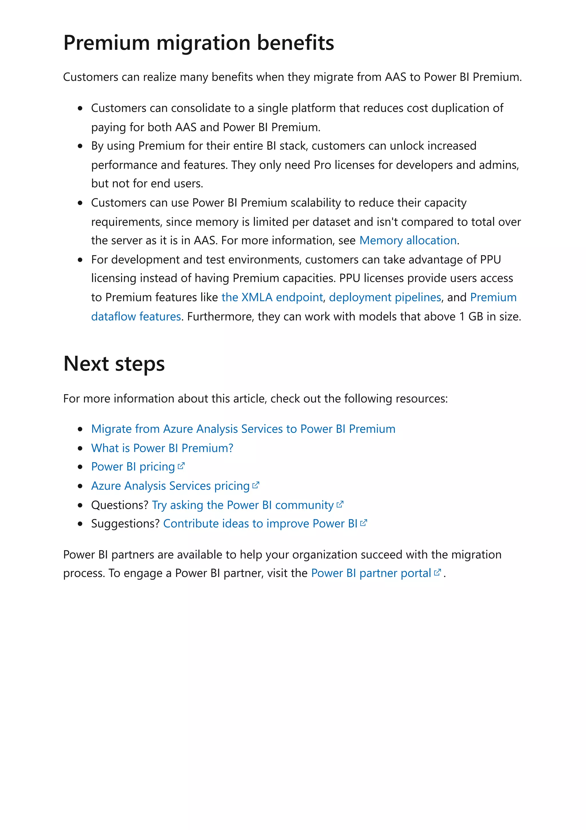
Let's see what happens when the Profit Margin measure is added to a table visual,
grouping by customer.
Sales (No Blank) =
IF(
ISBLANK([Sales]),
0,
[Sales]
)
Profit Margin =
DIVIDE([Profit], [Sales], 0)](https://image.slidesharecdn.com/docpower-bi-guidance-230227102019-b6273799/75/DOC-Power-Bi-Guidance-pdf-166-2048.jpg)
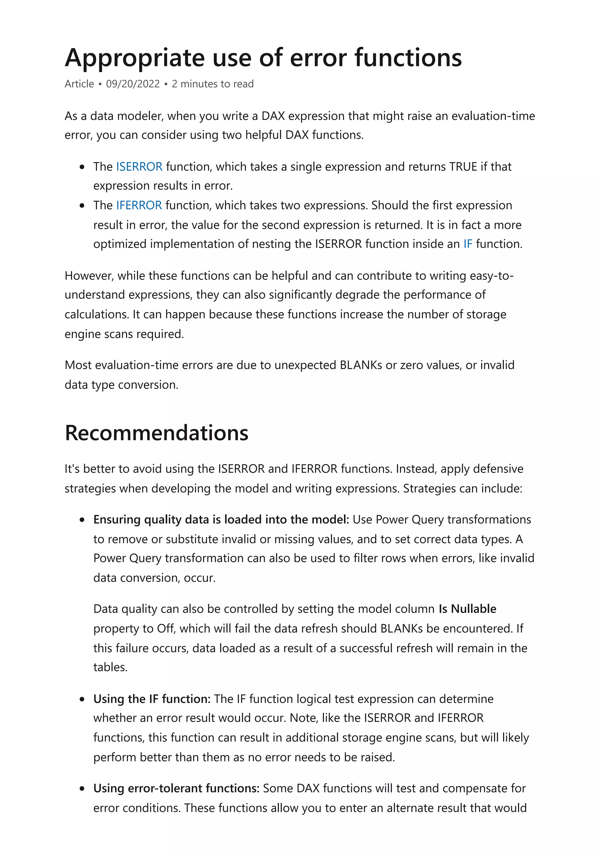
![The table visual displays an overwhelming number of rows. (There are in fact 18,484
customers in the model, and so the table attempts to display all of them.) Notice that
the customers in view haven't achieved any sales. Yet, because the Profit Margin
measure always returns a value, they are displayed.
Let's see what happens when the Profit Margin measure definition is improved. It now
returns a value only when the Sales measure isn't BLANK (or zero).
DAX
The table visual now displays only customers who have made sales within the current
filter context. The improved measure results in a more efficient and practical experience
for your report users.
7 Note
When there are too many data points to display in a visual, Power BI may use data
reduction strategies to remove or summarize large query results. For more
information, see Data point limits and strategies by visual type.
Profit Margin =
DIVIDE([Profit], [Sales])](https://image.slidesharecdn.com/docpower-bi-guidance-230227102019-b6273799/75/DOC-Power-Bi-Guidance-pdf-167-2048.jpg)
![Avoid using FILTER as a filter argument
Article • 09/20/2022 • 2 minutes to read
As a data modeler, it's common you'll write DAX expressions that need to be evaluated
in a modified filter context. For example, you can write a measure definition to calculate
sales for "high margin products". We'll describe this calculation later in this article.
The CALCULATE and CALCULATETABLE DAX functions are important and useful
functions. They let you write calculations that remove or add filters, or modify
relationship paths. It's done by passing in filter arguments, which are either Boolean
expressions, table expressions, or special filter functions. We'll only discuss Boolean and
table expressions in this article.
Consider the following measure definition, which calculates red product sales by using a
table expression. It will replace any filters that might be applied to the Product table.
DAX
The CALCULATE function accepts a table expression returned by the FILTER DAX
function, which evaluates its filter expression for each row of the Product table. It
achieves the correct result—the sales result for red products. However, it could be
achieved much more efficiently by using a Boolean expression.
Here's an improved measure definition, which uses a Boolean expression instead of the
table expression. The KEEPFILTERS DAX function ensures any existing filters applied to
the Color column are preserved, and not overwritten.
DAX
7 Note
This article is especially relevant for model calculations that apply filters to Import
tables.
Red Sales =
CALCULATE(
[Sales],
FILTER('Product', 'Product'[Color] = "Red")
)
Red Sales =
CALCULATE(
[Sales],](https://image.slidesharecdn.com/docpower-bi-guidance-230227102019-b6273799/75/DOC-Power-Bi-Guidance-pdf-169-2048.jpg)
![It's recommended you pass filter arguments as Boolean expressions, whenever possible.
It's because Import model tables are in-memory column stores. They are explicitly
optimized to efficiently filter columns in this way.
There are, however, restrictions that apply to Boolean expressions when they're used as
filter arguments. They:
Cannot reference columns from multiple tables
Cannot reference a measure
Cannot use nested CALCULATE functions
Cannot use functions that scan or return a table
It means that you'll need to use table expressions for more complex filter requirements.
Consider now a different measure definition. The requirement is to calculate sales, but
only for months that have achieved a profit.
DAX
In this example, the FILTER function must be used. It's because it requires evaluating the
Profit measure to eliminate those months that didn't achieve a profit. It's not possible to
use a measure in a Boolean expression when it's used as a filter argument.
For best performance, it's recommended you use Boolean expressions as filter
arguments, whenever possible.
Therefore, the FILTER function should only be used when necessary. You can use it to
perform filter complex column comparisons. These column comparisons can involve:
Measures
Other columns
KEEPFILTERS('Product'[Color] = "Red")
)
Sales for Profitable Months =
CALCULATE(
[Sales],
FILTER(
VALUES('Date'[Month]),
[Profit] > 0)
)
)
Recommendations](https://image.slidesharecdn.com/docpower-bi-guidance-230227102019-b6273799/75/DOC-Power-Bi-Guidance-pdf-170-2048.jpg)
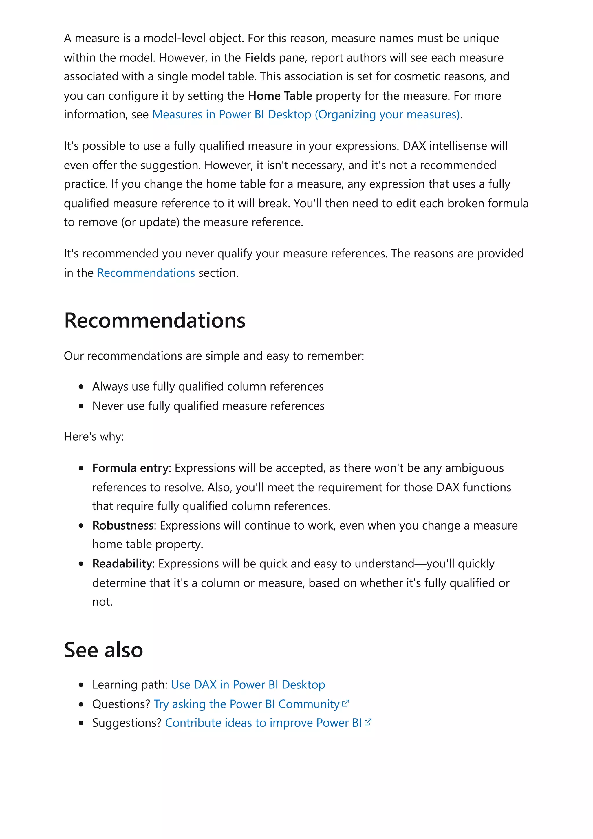
![Column and measure references
Article • 09/20/2022 • 2 minutes to read
As a data modeler, your DAX expressions will refer to model columns and measures.
Columns and measures are always associated with model tables, but these associations
are different, so we have different recommendations on how you'll reference them in
your expressions.
A column is a table-level object, and column names must be unique within a table. So
it's possible that the same column name is used multiple times in your model—
providing they belong to different tables. There's one more rule: a column name cannot
have the same name as a measure name or hierarchy name that exists in the same table.
In general, DAX will not force using a fully qualified reference to a column. A fully
qualified reference means that the table name precedes the column name.
Here's an example of a calculated column definition using only column name references.
The Sales and Cost columns both belong to a table named Orders.
DAX
The same definition can be rewritten with fully qualified column references.
DAX
Sometimes, however, you'll be required to use fully qualified column references when
Power BI detects ambiguity. When entering a formula, a red squiggly and error message
will alert you. Also, some DAX functions like the LOOKUPVALUE DAX function, require
the use of fully qualified columns.
It's recommended you always fully qualify your column references. The reasons are
provided in the Recommendations section.
Columns
Profit = [Sales] - [Cost]
Profit = Orders[Sales] - Orders[Cost]
Measures](https://image.slidesharecdn.com/docpower-bi-guidance-230227102019-b6273799/75/DOC-Power-Bi-Guidance-pdf-172-2048.jpg)
![DIVIDE function vs. divide operator (/)
Article • 09/20/2022 • 2 minutes to read
As a data modeler, when you write a DAX expression to divide a numerator by a
denominator, you can choose to use the DIVIDE function or the divide operator (/ -
forward slash).
When using the DIVIDE function, you must pass in numerator and denominator
expressions. Optionally, you can pass in a value that represents an alternate result.
DAX
The DIVIDE function was designed to automatically handle division by zero cases. If an
alternate result is not passed in, and the denominator is zero or BLANK, the function
returns BLANK. When an alternate result is passed in, it's returned instead of BLANK.
The DIVIDE function is convenient because it saves your expression from having to first
test the denominator value. The function is also better optimized for testing the
denominator value than the IF function. The performance gain is significant since
checking for division by zero is expensive. Further using DIVIDE results in a more concise
and elegant expression.
The following measure expression produces a safe division, but it involves using four
DAX functions.
DAX
This measure expression achieves the same outcome, yet more efficiently and elegantly.
DIVIDE(<numerator>, <denominator> [,<alternateresult>])
Example
Profit Margin =
IF(
OR(
ISBLANK([Sales]),
[Sales] == 0
),
BLANK(),
[Profit] / [Sales]
)](https://image.slidesharecdn.com/docpower-bi-guidance-230227102019-b6273799/75/DOC-Power-Bi-Guidance-pdf-174-2048.jpg)
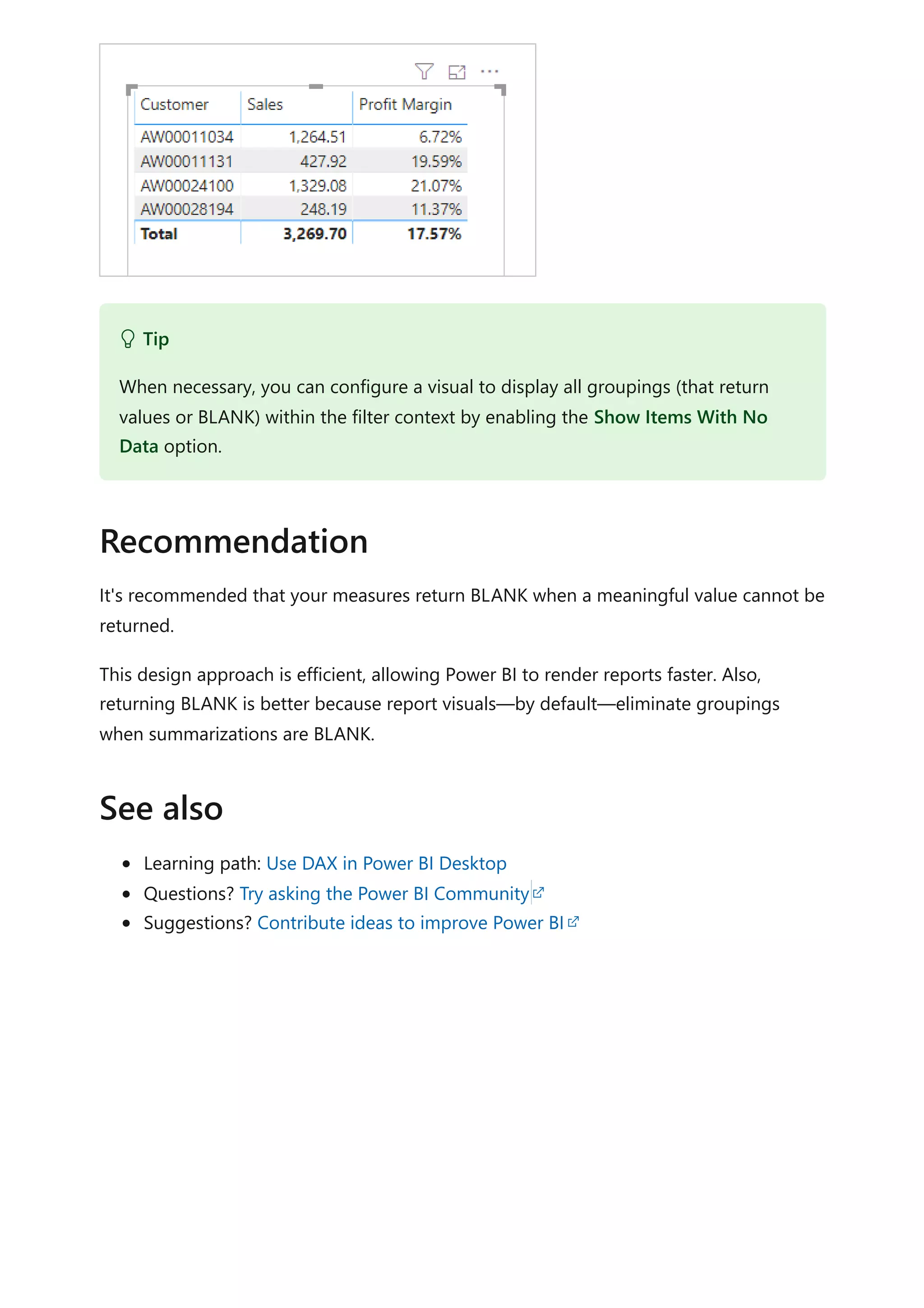
![DAX
It's recommended that you use the DIVIDE function whenever the denominator is an
expression that could return zero or BLANK.
In the case that the denominator is a constant value, we recommend that you use the
divide operator. In this case, the division is guaranteed to succeed, and your expression
will perform better because it will avoid unnecessary testing.
Carefully consider whether the DIVIDE function should return an alternate value. For
measures, it's usually a better design that they return BLANK. Returning BLANK is better
because report visuals—by default—eliminate groupings when summarizations are
BLANK. It allows the visual to focus attention on groups where data exists. When
necessary, in Power BI, you can configure the visual to display all groups (that return
values or BLANK) within the filter context by enabling the Show items with no data
option.
Learning path: Use DAX in Power BI Desktop
Questions? Try asking the Power BI Community
Suggestions? Contribute ideas to improve Power BI
Profit Margin =
DIVIDE([Profit], [Sales])
Recommendations
See also](https://image.slidesharecdn.com/docpower-bi-guidance-230227102019-b6273799/75/DOC-Power-Bi-Guidance-pdf-175-2048.jpg)
![Use COUNTROWS instead of COUNT
Article • 09/20/2022 • 2 minutes to read
As a data modeler, sometimes you might need to write a DAX expression that counts
table rows. The table could be a model table or an expression that returns a table.
Your requirement can be achieved in two ways. You can use the COUNT function to
count column values, or you can use the COUNTROWS function to count table rows.
Both functions will achieve the same result, providing that the counted column contains
no BLANKs.
The following measure definition presents an example. It calculates the number of
OrderDate column values.
DAX
Providing that the granularity of the Sales table is one row per sales order, and the
OrderDate column does not contain BLANKs, then the measure will return a correct
result.
However, the following measure definition is a better solution.
DAX
There are three reasons why the second measure definition is better:
It's more efficient, and so it will perform better.
It doesn't consider BLANKs contained in any column of the table.
The intention of formula is clearer, to the point of being self-describing.
When it's your intention to count table rows, it's recommended you always use the
COUNTROWS function.
Sales Orders =
COUNT(Sales[OrderDate])
Sales Orders =
COUNTROWS(Sales)
Recommendation](https://image.slidesharecdn.com/docpower-bi-guidance-230227102019-b6273799/75/DOC-Power-Bi-Guidance-pdf-176-2048.jpg)

![Use SELECTEDVALUE instead of VALUES
Article • 09/20/2022 • 2 minutes to read
As a data modeler, sometimes you might need to write a DAX expression that tests
whether a column is filtered by a specific value.
In earlier versions of DAX, this requirement was safely achieved by using a pattern
involving three DAX functions; IF, HASONEVALUE and VALUES. The following measure
definition presents an example. It calculates the sales tax amount, but only for sales
made to Australian customers.
DAX
In the example, the HASONEVALUE function returns TRUE only when a single value of
the Country-Region column is visible in the current filter context. When it's TRUE, the
VALUES function is compared to the literal text "Australia". When the VALUES function
returns TRUE, the Sales measure is multiplied by 0.10 (representing 10%). If the
HASONEVALUE function returns FALSE—because more than one value filters the column
—the first IF function returns BLANK.
The use of the HASONEVALUE is a defensive technique. It's required because it's
possible that multiple values filter the Country-Region column. In this case, the VALUES
function returns a table of multiple rows. Comparing a table of multiple rows to a scalar
value results in an error.
It's recommended that you use the SELECTEDVALUE function. It achieves the same
outcome as the pattern described in this article, yet more efficiently and elegantly.
Using the SELECTEDVALUE function, the example measure definition is now rewritten.
DAX
Australian Sales Tax =
IF(
HASONEVALUE(Customer[Country-Region]),
IF(
VALUES(Customer[Country-Region]) = "Australia",
[Sales] * 0.10
)
)
Recommendation](https://image.slidesharecdn.com/docpower-bi-guidance-230227102019-b6273799/75/DOC-Power-Bi-Guidance-pdf-178-2048.jpg)
![Learning path: Use DAX in Power BI Desktop
Questions? Try asking the Power BI Community
Suggestions? Contribute ideas to improve Power BI
Australian Sales Tax =
IF(
SELECTEDVALUE(Customer[Country-Region]) = "Australia",
[Sales] * 0.10
)
Tip
It's possible to pass an alternate result value into the SELECTEDVALUE function. The
alternate result value is returned when either no filters—or multiple filters—are
applied to the column.
See also](https://image.slidesharecdn.com/docpower-bi-guidance-230227102019-b6273799/75/DOC-Power-Bi-Guidance-pdf-179-2048.jpg)
![Use variables to improve your DAX
formulas
Article • 10/31/2022 • 3 minutes to read
As a data modeler, writing and debugging some DAX calculations can be challenging.
It's common that complex calculation requirements often involve writing compound or
complex expressions. Compound expressions can involve the use of many nested
functions, and possibly the reuse of expression logic.
Using variables in your DAX formulas can help you write more complex and efficient
calculations. Variables can improve performance, reliability, readability, and reduce
complexity.
In this article, we'll demonstrate the first three benefits by using an example measure for
year-over-year (YoY) sales growth. (The formula for YoY sales growth is period sales,
minus sales for the same period last year, divided by sales for the same period last year.)
Let's start with the following measure definition.
DAX
The measure produces the correct result, yet let's now see how it can be improved.
Notice that the formula repeats the expression that calculates "same period last year".
This formula is inefficient, as it requires Power BI to evaluate the same expression twice.
The measure definition can be made more efficient by using a variable, VAR.
The following measure definition represents an improvement. It uses an expression to
assign the "same period last year" result to a variable named SalesPriorYear. The
variable is then used twice in the RETURN expression.
DAX
Sales YoY Growth % =
DIVIDE(
([Sales] - CALCULATE([Sales], PARALLELPERIOD('Date'[Date], -12,
MONTH))),
CALCULATE([Sales], PARALLELPERIOD('Date'[Date], -12, MONTH))
)
Improve performance](https://image.slidesharecdn.com/docpower-bi-guidance-230227102019-b6273799/75/DOC-Power-Bi-Guidance-pdf-180-2048.jpg)
![The measure continues to produce the correct result, and does so in about half the
query time.
In the previous measure definition, notice how the choice of variable name makes the
RETURN expression simpler to understand. The expression is short and self-describing.
Variables can also help you debug a formula. To test an expression assigned to a
variable, you temporarily rewrite the RETURN expression to output the variable.
The following measure definition returns only the SalesPriorYear variable. Notice how it
comments-out the intended RETURN expression. This technique allows you to easily
revert it back once your debugging is complete.
DAX
In earlier versions of DAX, variables were not yet supported. Complex expressions that
introduced new filter contexts were required to use the EARLIER or EARLIEST DAX
functions to reference outer filter contexts. Unfortunately, data modelers found these
functions difficult to understand and use.
Variables are always evaluated outside the filters your RETURN expression applies. For
this reason, when you use a variable within a modified filter context, it achieves the
same result as the EARLIEST function. The use of the EARLIER or EARLIEST functions can
Sales YoY Growth % =
VAR SalesPriorYear =
CALCULATE([Sales], PARALLELPERIOD('Date'[Date], -12, MONTH))
RETURN
DIVIDE(([Sales] - SalesPriorYear), SalesPriorYear)
Improve readability
Simplify debugging
Sales YoY Growth % =
VAR SalesPriorYear =
CALCULATE([Sales], PARALLELPERIOD('Date'[Date], -12, MONTH))
RETURN
--DIVIDE(([Sales] - SalesPriorYear), SalesPriorYear)
SalesPriorYear
Reduce complexity](https://image.slidesharecdn.com/docpower-bi-guidance-230227102019-b6273799/75/DOC-Power-Bi-Guidance-pdf-181-2048.jpg)
![therefore be avoided. It means you can now write formulas that are less complex, and
that are easier to understand.
Consider the following calculated column definition added to the Subcategory table. It
evaluates a rank for each product subcategory based on the Subcategory Sales column
values.
DAX
The EARLIER function is used to refer to the Subcategory Sales column value in the
current row context.
The calculated column definition can be improved by using a variable instead of the
EARLIER function. The CurrentSubcategorySales variable stores the Subcategory Sales
column value in the current row context, and the RETURN expression uses it within a
modified filter context.
DAX
VAR DAX article
Learning path: Use DAX in Power BI Desktop
Questions? Try asking the Power BI Community
Subcategory Sales Rank =
COUNTROWS(
FILTER(
Subcategory,
EARLIER(Subcategory[Subcategory Sales]) < Subcategory[Subcategory
Sales]
)
) + 1
Subcategory Sales Rank =
VAR CurrentSubcategorySales = Subcategory[Subcategory Sales]
RETURN
COUNTROWS(
FILTER(
Subcategory,
CurrentSubcategorySales < Subcategory[Subcategory Sales]
)
) + 1
See also](https://image.slidesharecdn.com/docpower-bi-guidance-230227102019-b6273799/75/DOC-Power-Bi-Guidance-pdf-182-2048.jpg)

![3. Create the StateProvince dataset that retrieves distinct state-province values for
the selected country-region, using the following query statement:
SQL
4. Create the City dataset that retrieves distinct city values for the selected country-
region and state-province, using the following query statement:
SQL
5. Continue this pattern to create the PostalCode dataset.
6. Create the Reseller dataset to retrieve all resellers for the selected geographic
values, using the following query statement:
SQL
SELECT DISTINCT
[Country-Region]
FROM
[Reseller]
ORDER BY
[Country-Region]
SELECT DISTINCT
[State-Province]
FROM
[Reseller]
WHERE
[Country-Region] = @CountryRegion
ORDER BY
[State-Province]
SELECT DISTINCT
[City]
FROM
[Reseller]
WHERE
[Country-Region] = @CountryRegion
AND [State-Province] = @StateProvince
ORDER BY
[City]
SELECT
[ResellerCode],
[ResellerName]
FROM
[Reseller]](https://image.slidesharecdn.com/docpower-bi-guidance-230227102019-b6273799/75/DOC-Power-Bi-Guidance-pdf-210-2048.jpg)
![7. For each dataset except the first, map the query parameters to the corresponding
report parameters.
In this example, the report user interacts with a report parameter to select the first letter
of the reseller. A second parameter then lists resellers when the name commences with
the selected letter.
Here's how you can develop the cascading parameters:
WHERE
[Country-Region] = @CountryRegion
AND [State-Province] = @StateProvince
AND [City] = @City
AND [PostalCode] = @PostalCode
ORDER BY
[ResellerName]
7 Note
All query parameters (prefixed with the @ symbol) shown in these examples could
be embedded within SELECT statements, or passed to stored procedures.
Generally, stored procedures are a better design approach. It's because their query
plans are cached for quicker execution, and they allow you develop more
sophisticated logic, when needed. However, they aren't currently supported for
gateway relational data sources, which means SQL Server, Oracle, and Teradata.
Lastly, you should always ensure suitable indexes exist to support efficient data
retrieval. Otherwise, your report parameters could be slow to populate, and the
database could become overburdened. For more information about SQL Server
indexing, see SQL Server Index Architecture and Design Guide.
Filter by a grouping column](https://image.slidesharecdn.com/docpower-bi-guidance-230227102019-b6273799/75/DOC-Power-Bi-Guidance-pdf-211-2048.jpg)
![1. Create the ReportGroup and Reseller report parameters, ordered in the correct
sequence.
2. Create the ReportGroup dataset to retrieve the first letters used by all resellers,
using the following query statement:
SQL
3. Create the Reseller dataset to retrieve all resellers that commence with the
selected letter, using the following query statement:
SQL
4. Map the query parameter of the Reseller dataset to the corresponding report
parameter.
It's more efficient to add the grouping column to the Reseller table. When persisted and
indexed, it delivers the best result. For more information, see Specify Computed
Columns in a Table.
SQL
This technique can deliver even greater potential. Consider the following script that adds
a new grouping column to filter resellers by pre-defined bands of letters. It also creates
an index to efficiently retrieve the data required by the report parameters.
SQL
SELECT DISTINCT
LEFT([ResellerName], 1) AS [ReportGroup]
FROM
[Reseller]
ORDER BY
[ReportGroup]
SELECT
[ResellerCode],
[ResellerName]
FROM
[Reseller]
WHERE
LEFT([ResellerName], 1) = @ReportGroup
ORDER BY
[ResellerName]
ALTER TABLE [Reseller]
ADD [ReportGroup] AS LEFT([ResellerName], 1) PERSISTED](https://image.slidesharecdn.com/docpower-bi-guidance-230227102019-b6273799/75/DOC-Power-Bi-Guidance-pdf-212-2048.jpg)
![In this example, the report user interacts with a report parameter to enter a search
pattern. A second parameter then lists resellers when the name contains the pattern.
Here's how you can develop the cascading parameters:
1. Create the Search and Reseller report parameters, ordered in the correct sequence.
2. Create the Reseller dataset to retrieve all resellers that contain the search text,
using the following query statement:
SQL
ALTER TABLE [Reseller]
ADD [ReportGroup2] AS CASE
WHEN [ResellerName] LIKE '[A-C]%' THEN 'A-C'
WHEN [ResellerName] LIKE '[D-H]%' THEN 'D-H'
WHEN [ResellerName] LIKE '[I-M]%' THEN 'I-M'
WHEN [ResellerName] LIKE '[N-S]%' THEN 'N-S'
WHEN [ResellerName] LIKE '[T-Z]%' THEN 'T-Z'
ELSE '[Other]'
END PERSISTED
GO
CREATE NONCLUSTERED INDEX [Reseller_ReportGroup2]
ON [Reseller] ([ReportGroup2]) INCLUDE ([ResellerCode], [ResellerName])
GO
Filter by search pattern
SELECT
[ResellerCode],
[ResellerName]
FROM
[Reseller]
WHERE
[ResellerName] LIKE '%' + @Search + '%'
ORDER BY
[ResellerName]](https://image.slidesharecdn.com/docpower-bi-guidance-230227102019-b6273799/75/DOC-Power-Bi-Guidance-pdf-213-2048.jpg)
![3. Map the query parameter of the Reseller dataset to the corresponding report
parameter.
Here's how you can let the report users define their own pattern.
SQL
Many non-database professionals, however, don't know about the percentage (%)
wildcard character. Instead, they're familiar with the asterisk (*) character. By modifying
the WHERE clause, you can let them use this character.
SQL
In this scenario, you can use fact data to limit available values. Report users will be
presented with items where activity has been recorded.
In this example, the report user interacts with three report parameter. The first two set a
date range of sales order dates. The third parameter then lists resellers where orders
have been created during that time period.
Tip
You can improve upon this design to provide more control for your report users. It
lets them define their own pattern matching value. For example, the search value
"red%" will filter to resellers with names that commence with the characters "red".
For more information, see LIKE (Transact-SQL).
WHERE
[ResellerName] LIKE @Search
WHERE
[ResellerName] LIKE SUBSTITUTE(@Search, '%', '*')
Present relevant items](https://image.slidesharecdn.com/docpower-bi-guidance-230227102019-b6273799/75/DOC-Power-Bi-Guidance-pdf-214-2048.jpg)
![Here's how you can develop the cascading parameters:
1. Create the OrderDateStart, OrderDateEnd, and Reseller report parameters,
ordered in the correct sequence.
2. Create the Reseller dataset to retrieve all resellers that created orders in the date
period, using the following query statement:
SQL
We recommend you design your reports with cascading parameters, whenever possible.
It's because they:
Provide intuitive and helpful experiences for your report users
Are efficient, because they retrieve smaller sets of available values
Be sure to optimize your data sources by:
Using stored procedures, whenever possible
Adding appropriate indexes for efficient data retrieval
SELECT DISTINCT
[r].[ResellerCode],
[r].[ResellerName]
FROM
[Reseller] AS [r]
INNER JOIN [Sales] AS [s]
ON [s].[ResellerCode] = [r].[ResellerCode]
WHERE
[s].[OrderDate] >= @OrderDateStart
AND [s].[OrderDate] < DATEADD(DAY, 1, @OrderDateEnd)
ORDER BY
[r].[ResellerName]
Recommendations](https://image.slidesharecdn.com/docpower-bi-guidance-230227102019-b6273799/75/DOC-Power-Bi-Guidance-pdf-215-2048.jpg)


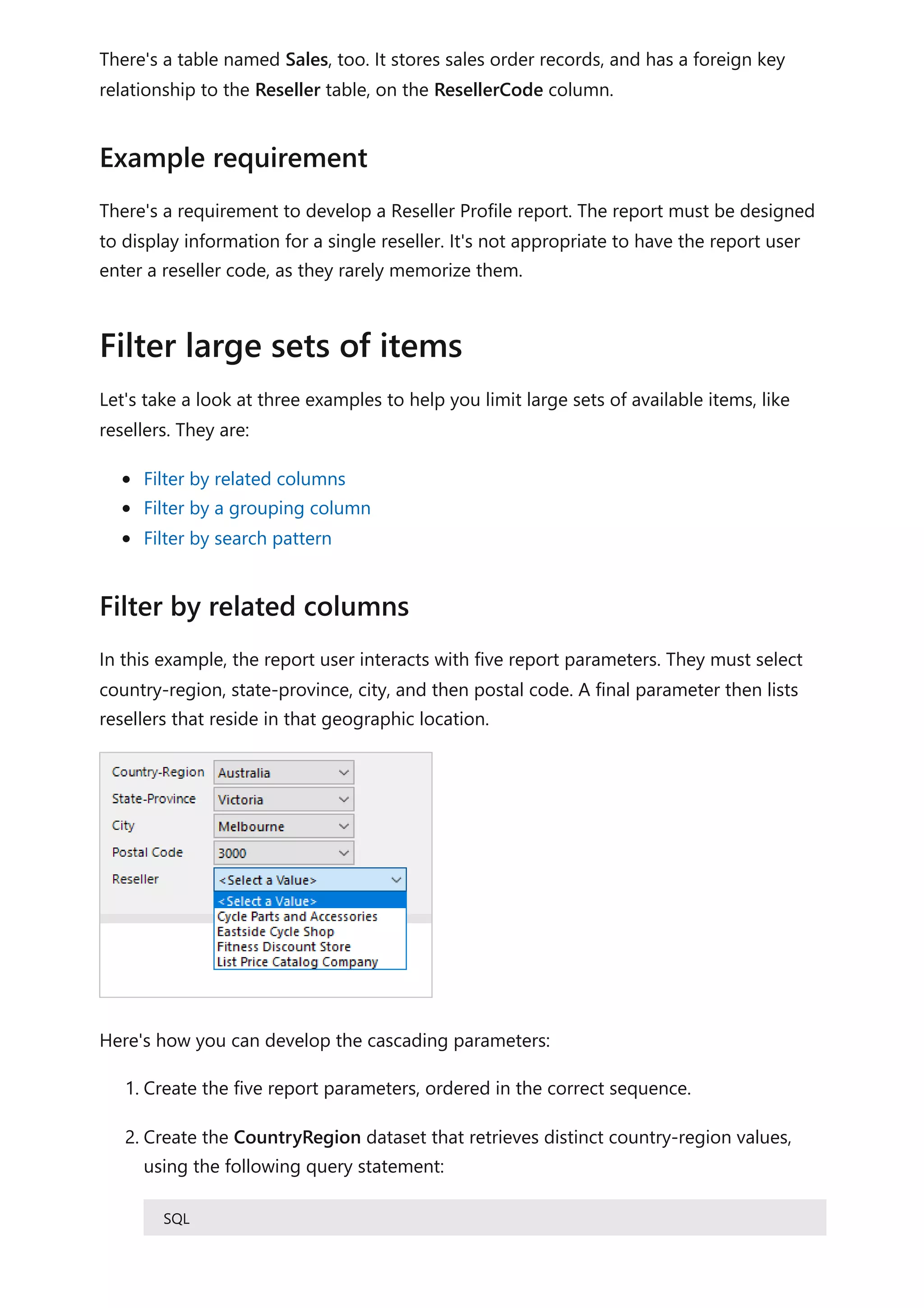
![1. Open your Power BI Desktop report (so it will be easy to locate the port in the next
step, close any other open reports).
2. To determine the port being used by Power BI Desktop, in PowerShell (with
administrator privileges), or at the Command Prompt, enter the following
command:
PowerShell
The output will be a list of applications and their open ports. Look for the port
used by msmdsrv.exe, and record it for later use. It's your instance of Power BI
Desktop.
3. To connect SQL Server Profiler to your Power BI Desktop report:
a. Open SQL Server Profiler.
b. In SQL Server Profiler, on the File menu, select New Trace.
c. For Server Type, select Analysis Services.
d. For Server Name, enter localhost:[port recorded earlier].
e. Click Run—now the SQL Server Profiler trace is live, and is actively profiling
Power BI Desktop queries.
4. As Power BI Desktop queries are executed, you'll see their respective durations and
CPU times. Depending on the data source type, you may see other events
indicating how the query was executed. Using this information, you can determine
which queries are the bottlenecks.
A benefit of using SQL Server Profiler is that it's possible to save a SQL Server (relational)
database trace. The trace can become an input to the Database Engine Tuning Advisor.
This way, you can receive recommendations on how to tune your data source.
Monitor performance of content deployed into your organization's Power BI Premium
capacity with the help of the Premium metrics app.
For more information about this article, check out the following resources:
Query Diagnostics
Performance Analyzer
Troubleshoot report performance in Power BI
Power BI Premium Metrics app
netstat -b -n
Monitor Premium metrics
Next steps](https://image.slidesharecdn.com/docpower-bi-guidance-230227102019-b6273799/75/DOC-Power-Bi-Guidance-pdf-262-2048.jpg)


![PowerShell
# Written by Sergei Gundorov; v1 development started on 07/08/2020
#
# Intent: 1. Address common friction points and usage issues and questions
related to the
# events generated by Power BI Service that are stored in the
activity log.
# 2. Provide boiler plate code for capturing all 30 days of
available data.
# 3. Power BI admin privileges are required to use the Activity Log
API.
#
# Use: Sign in to the Power BI service with admin privileges and execute
specific segment one at a time.
# IMPORTANT: Use Connect-PowerBIServiceAccount to connect to the service
before running individual code segments.
# IMPORTANT: $day value may need to be adjusted depending on where you're
located in the world relative to UTC.
# The Power BI activity log records events using UTC time; so add
or subtract days according to your global location.
# SCENARIO: Sample code fragment to retrieve a limited number of attributes
for specific events for specific user report viewing activity.
# You need to get user's Azure Active Directory (AAD) object ID. You can use
this Azure AD cmdlet:
https://learn.microsoft.com/powershell/module/azuread/get-azureaduser?
view=azureadps-2.0
# Dates need to be entered using ISO 8601 format; adjust dates to span no
more than 24 hours.
$a=Get-PowerBIActivityEvent -StartDateTime '2020-06-23T19:00:00.000' -
EndDateTime '2020-06-23T20:59:59.999' -ActivityType 'ViewReport' -User [USER
AAD ObjectId GUID] | ConvertFrom-Json
# You can use any attribute value to filter results further. For example, a
specific event request Id can be used to analyze just one specific event.
$a | Select RequestId, ReportName, WorkspaceName |where {($_.RequestId -eq
'[RequestId GUID of the event]')}
# SCENARIO: Retrieve a list of users for specific app.
# The user list can be partially derived (based on last 30 days of available
activity) by combining data for two events: CreateApp and UpdateApp.
# Both events will contain OrgAppPermission property that contains app user
access list.
# Actual app installation can be tracked using InstallApp activity.
# Run each code segment separately for each event.
# Iterate through 30 days of activity CreateApp.
$day=Get-date](https://image.slidesharecdn.com/docpower-bi-guidance-230227102019-b6273799/75/DOC-Power-Bi-Guidance-pdf-277-2048.jpg)
![for($s=0; $s -le 30; $s++)
{
$periodStart=$day.AddDays(-$s)
$base=$periodStart.ToString("yyyy-MM-dd")
write-host $base
$a=Get-PowerBIActivityEvent -StartDateTime ($base+'T00:00:00.000') -
EndDateTime ($base+'T23:59:59.999') -ActivityType 'CreateApp' -ResultType
JsonString | ConvertFrom-Json
$c=$a.Count
for($i=0 ; $i -lt $c; $i++)
{
$r=$a[$i]
Write-Host "App Name `t: $($r.ItemName)"
` "WS Name `t: $($r.WorkSpaceName)"
` "WS ID `t`t: $($r.WorkspaceId)"
` "Created `t: $($r.CreationTime)"
` "Users `t`t: $($r.OrgAppPermission) `n"
}
}
# Iterate through 30 days of activity UpdateApp.
$day=Get-date
for($s=0; $s -le 30; $s++)
{
$periodStart=$day.AddDays(-$s)
$base=$periodStart.ToString("yyyy-MM-dd")
write-host $base
$a=Get-PowerBIActivityEvent -StartDateTime ($base+'T00:00:00.000') -
EndDateTime ($base+'T23:59:59.999') -ActivityType 'UpdateApp' -ResultType
JsonString | ConvertFrom-Json
$c=$a.Count
for($i=0 ; $i -lt $c; $i++)
{
$r=$a[$i]
Write-Host "App Name `t: $($r.ItemName)"
` "WS Name `t: $($r.WorkSpaceName)"
` "WS ID `t`t: $($r.WorkspaceId)"
` "Updated `t: $($r.CreationTime)"
` "Users `t`t: $($r.OrgAppPermission) `n"
}
}
# Iterate through 30 days of activity InstallApp.
$day=Get-date
for($s=0; $s -le 30; $s++)
{
$periodStart=$day.AddDays(-$s)](https://image.slidesharecdn.com/docpower-bi-guidance-230227102019-b6273799/75/DOC-Power-Bi-Guidance-pdf-278-2048.jpg)
![$base=$periodStart.ToString("yyyy-MM-dd")
write-host $base
$a=Get-PowerBIActivityEvent -StartDateTime ($base+'T00:00:00.000') -
EndDateTime ($base+'T23:59:59.999') -ActivityType 'InstallApp' -ResultType
JsonString | ConvertFrom-Json
$c=$a.Count
for($i=0 ; $i -lt $c; $i++)
{
$r=$a[$i]
Write-Host "App Name `t: $($r.ItemName)"
` "Installed `t: $($r.CreationTime)"
` "User `t`t: $($r.UserId) `n"
}
}
# SCENARIO: Retrieve a list of users for direct report sharing.
# This logic and flow can be used for tracing direct dashboard sharing by
substituting activity type.
# Default output is formatted to return the list of users as a string. There
is commented out code block to get multi-line user list.
# IMPORTANT: Removal of a user or group from direct sharing access list
event is not tracked. For this reason, the list may be not accurate.
# IMPORTANT: If the user list contains a GUID instead of a UPN the report
was shared to a group.
# Group name and email can be obtained using Azure AD cmdlets
using captured ObjectId GUID.
# Iterate through 30 days of activity ShareReport.
$day=Get-date
for($s=0; $s -le 30; $s++)
{
$periodStart=$day.AddDays(-$s)
$base=$periodStart.ToString("yyyy-MM-dd")
#write-host $base
$a=Get-PowerBIActivityEvent -StartDateTime ($base+'T00:00:00.000') -
EndDateTime ($base+'T23:59:59.999') -ActivityType 'ShareReport' -ResultType
JsonString | ConvertFrom-Json
$c=$a.Count
for($i=0 ; $i -lt $c; $i++)
{
$r=$a[$i]
Write-Host "Rpt Name `t: $($r.ItemName)"
` "Rpt Id `t: $($r.ArtifactId)"
` "WS Name `t: $($r.WorkSpaceName)"
` "WS ID `t`t: $($r.WorkspaceId)"
` "Capacity `t: $($r.CapacityId)"
` "SharedOn `t: $($r.CreationTime.Replace('T','](https://image.slidesharecdn.com/docpower-bi-guidance-230227102019-b6273799/75/DOC-Power-Bi-Guidance-pdf-279-2048.jpg)
![For more information related to this article, check out the following resources:
Track user activities in Power BI
Questions? Try asking the Power BI Community
Suggestions? Contribute ideas to improve Power BI
').Replace('Z',''))"
` "User `t`t: $($r.UserId)"
# NOTE: $_.RecipientEmail + $_.RecipientName or
+$_.ObjectId is the case for group sharing
# can never happen both at the same time in the
same JSON record
` "Shared with`t: $(($r.SharingInformation)| %
{$_.RecipientEmail + $_.ObjectId +'[' + $_.ResharePermission +']'})"
#OPTIONAL: Formatted output for SharingInformation attribute
#$sc= $r.SharingInformation.Count
#Write-Host "Shared with`t:"
#for($j=0;$j -lt $sc;$j++)
#{
# Write-Host "`t`t`t
$($r.SharingInformation[$j].RecipientEmail)" -NoNewline
# Write-Host $r.SharingInformation[$j].ObjectId -NoNewline
# Write-Host ('[' + $r.SharingInformation[$j].ResharePermission
+']')
#}
Write-host ""
}
}
Next steps](https://image.slidesharecdn.com/docpower-bi-guidance-230227102019-b6273799/75/DOC-Power-Bi-Guidance-pdf-280-2048.jpg)
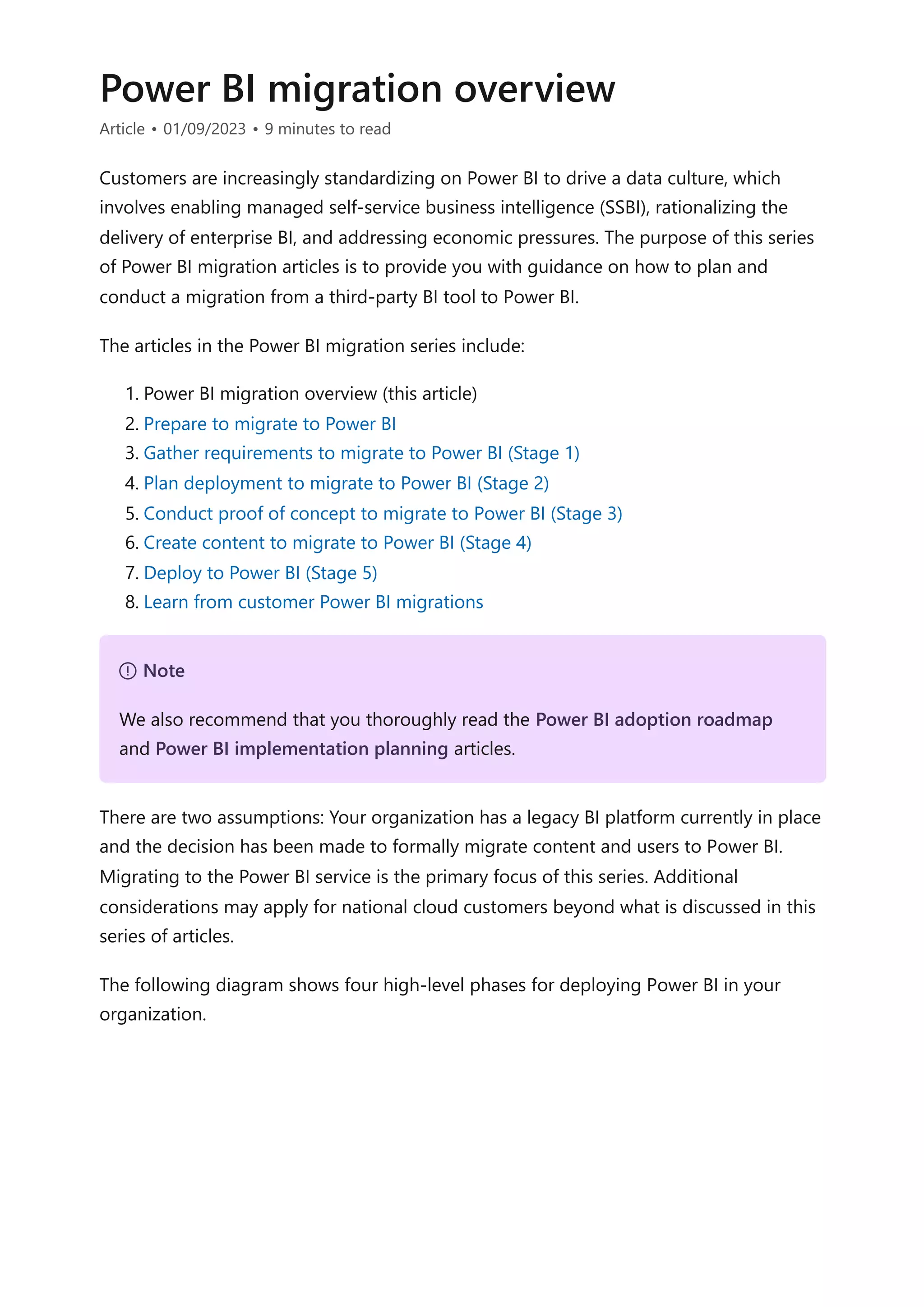
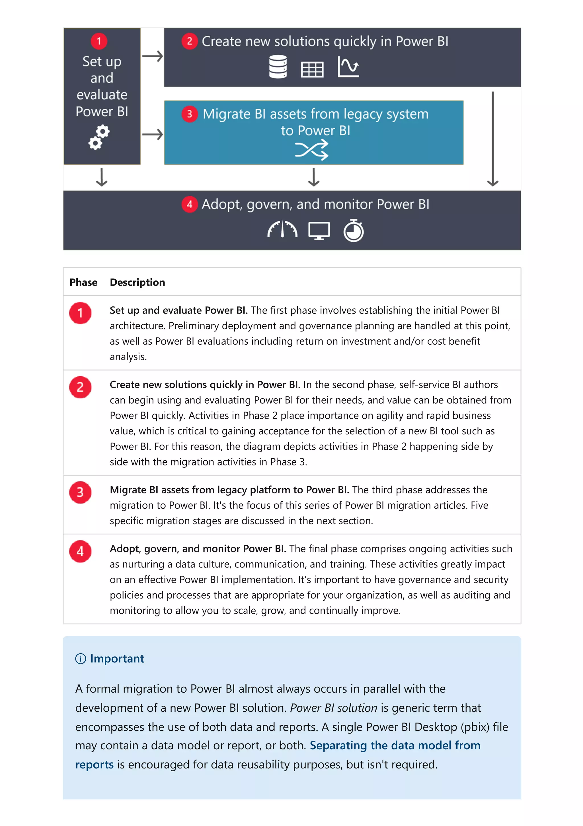
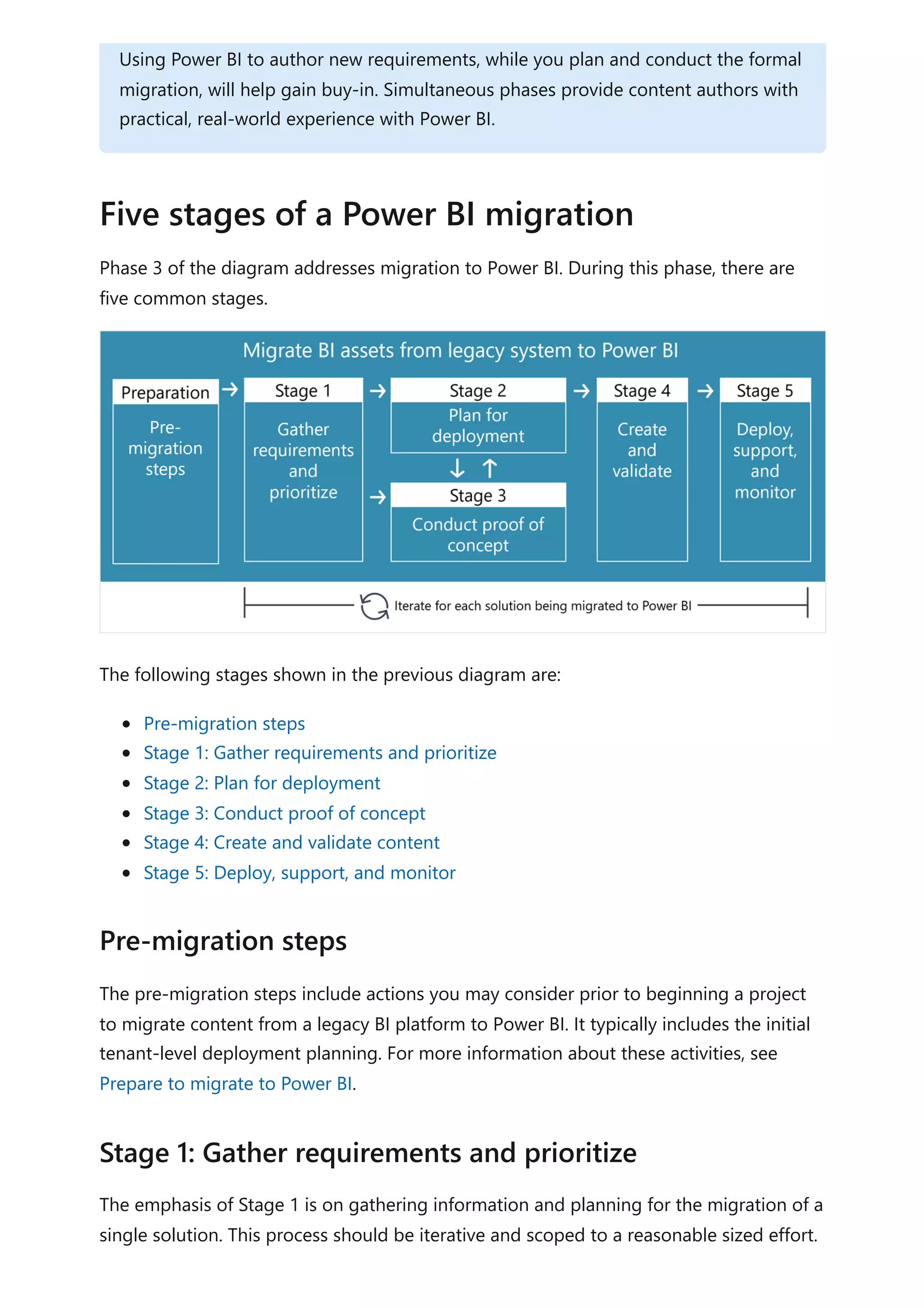

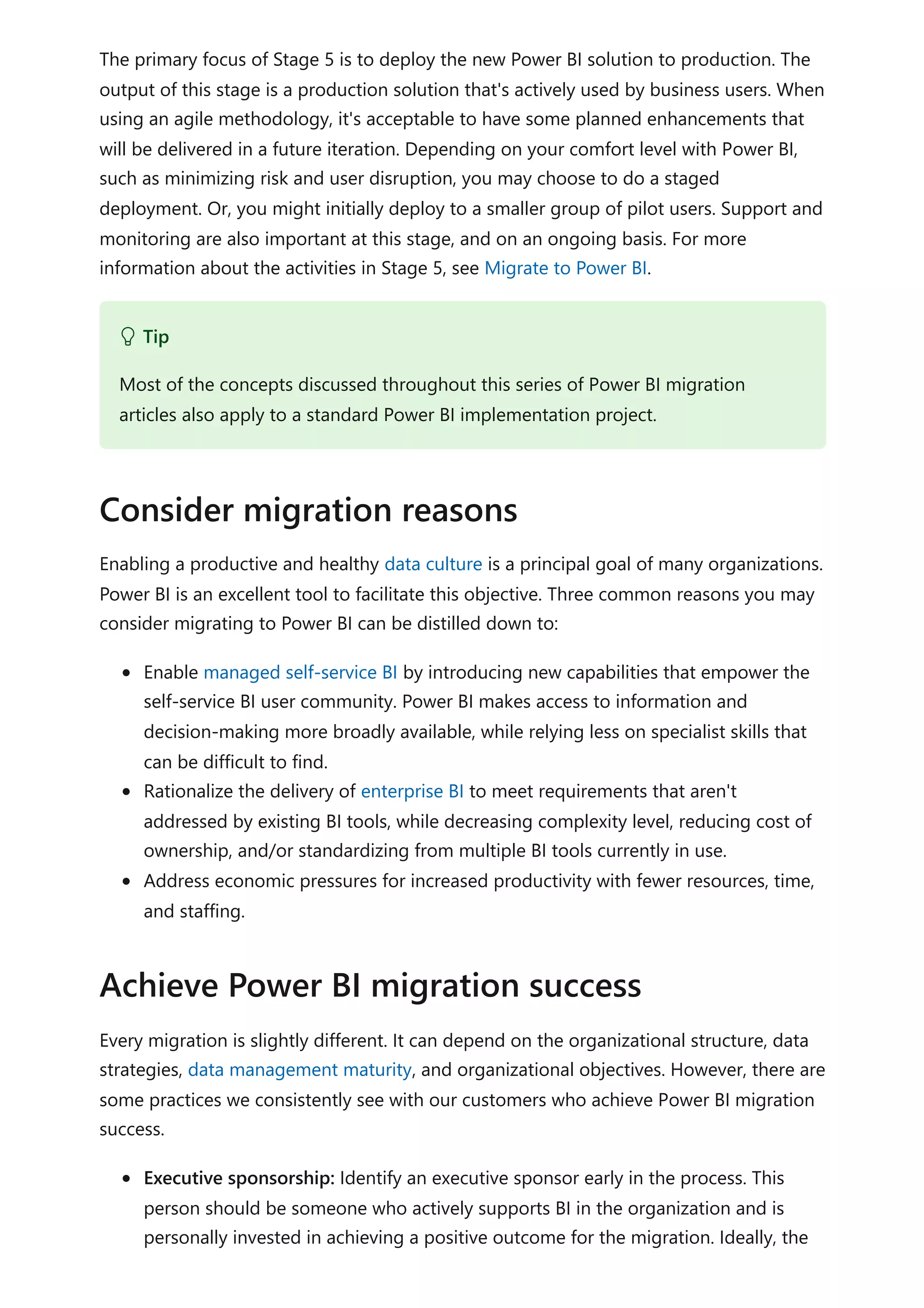
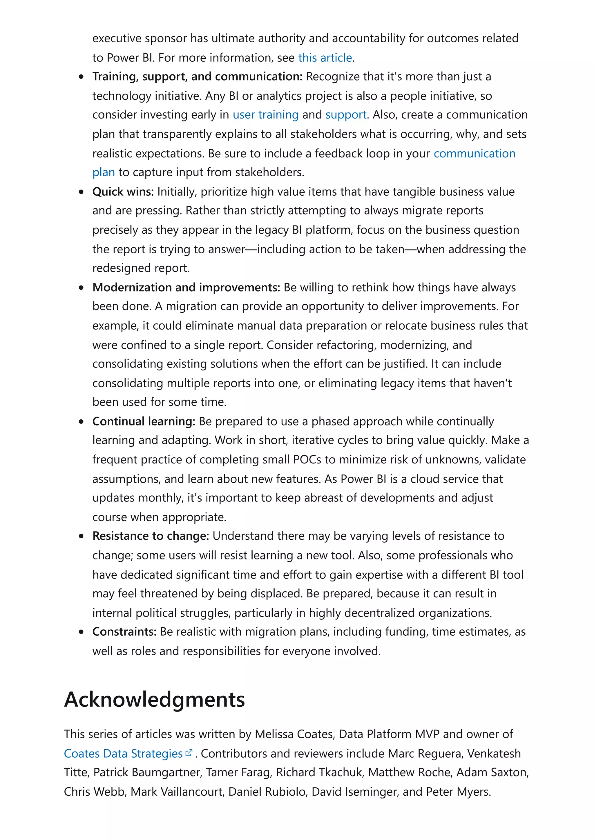
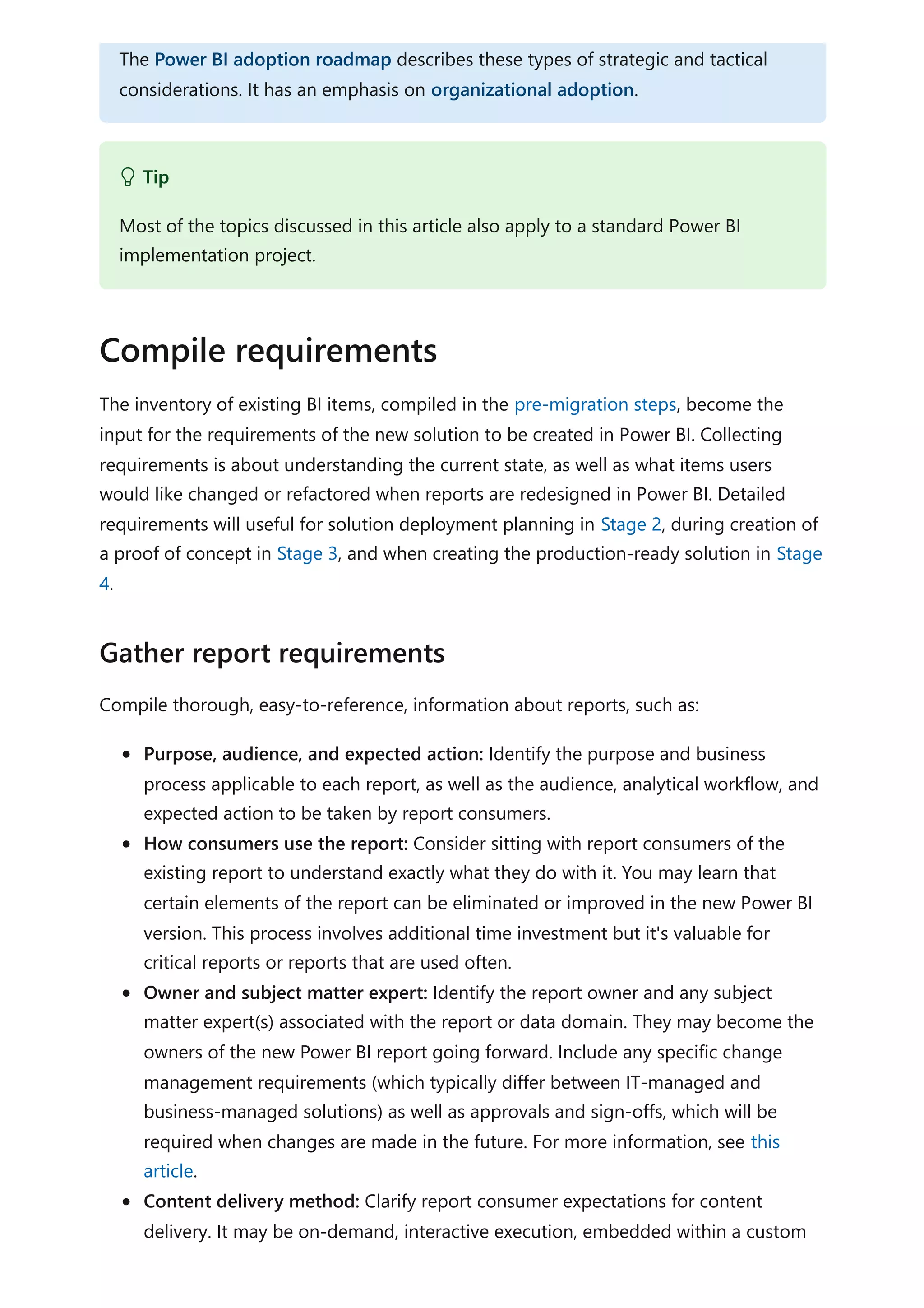

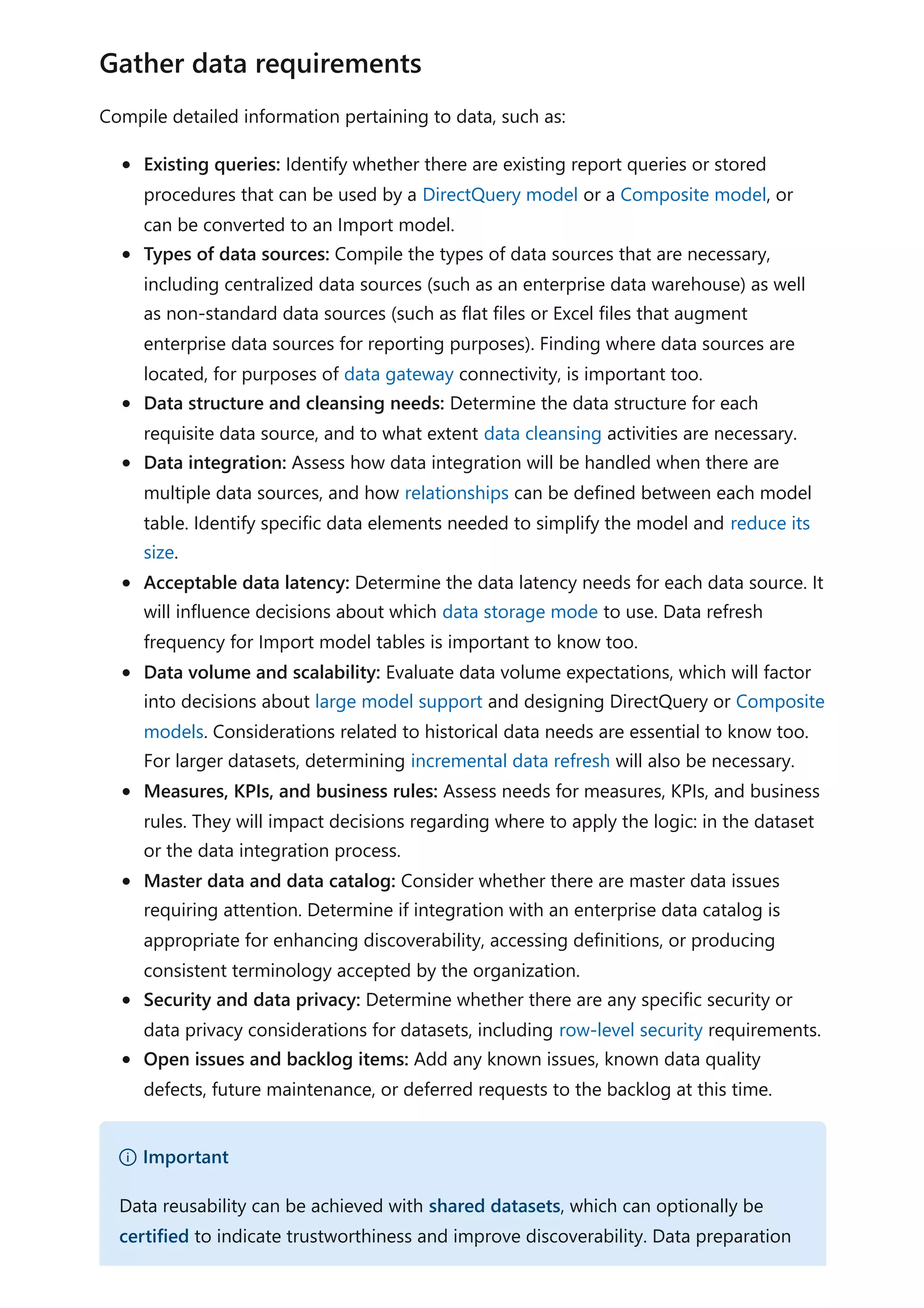
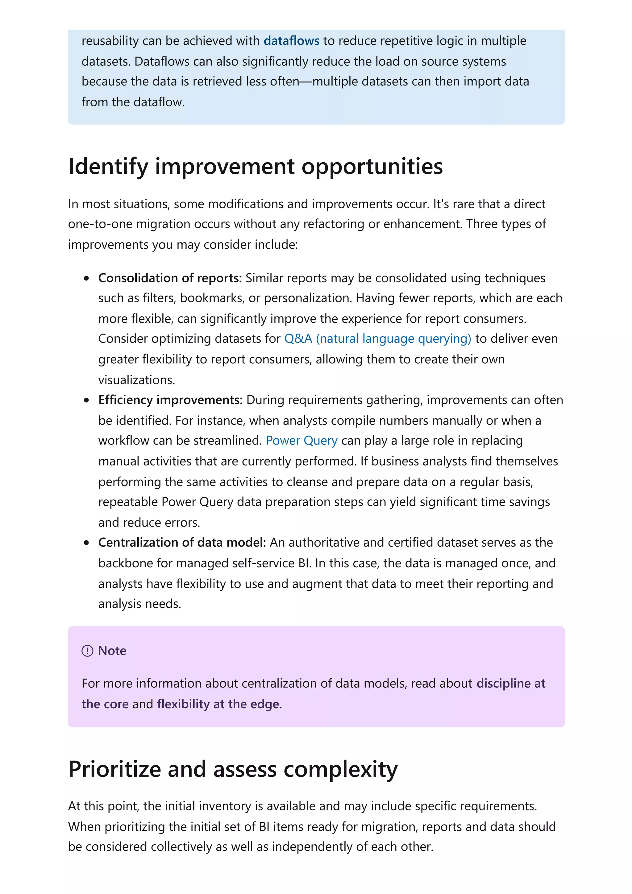
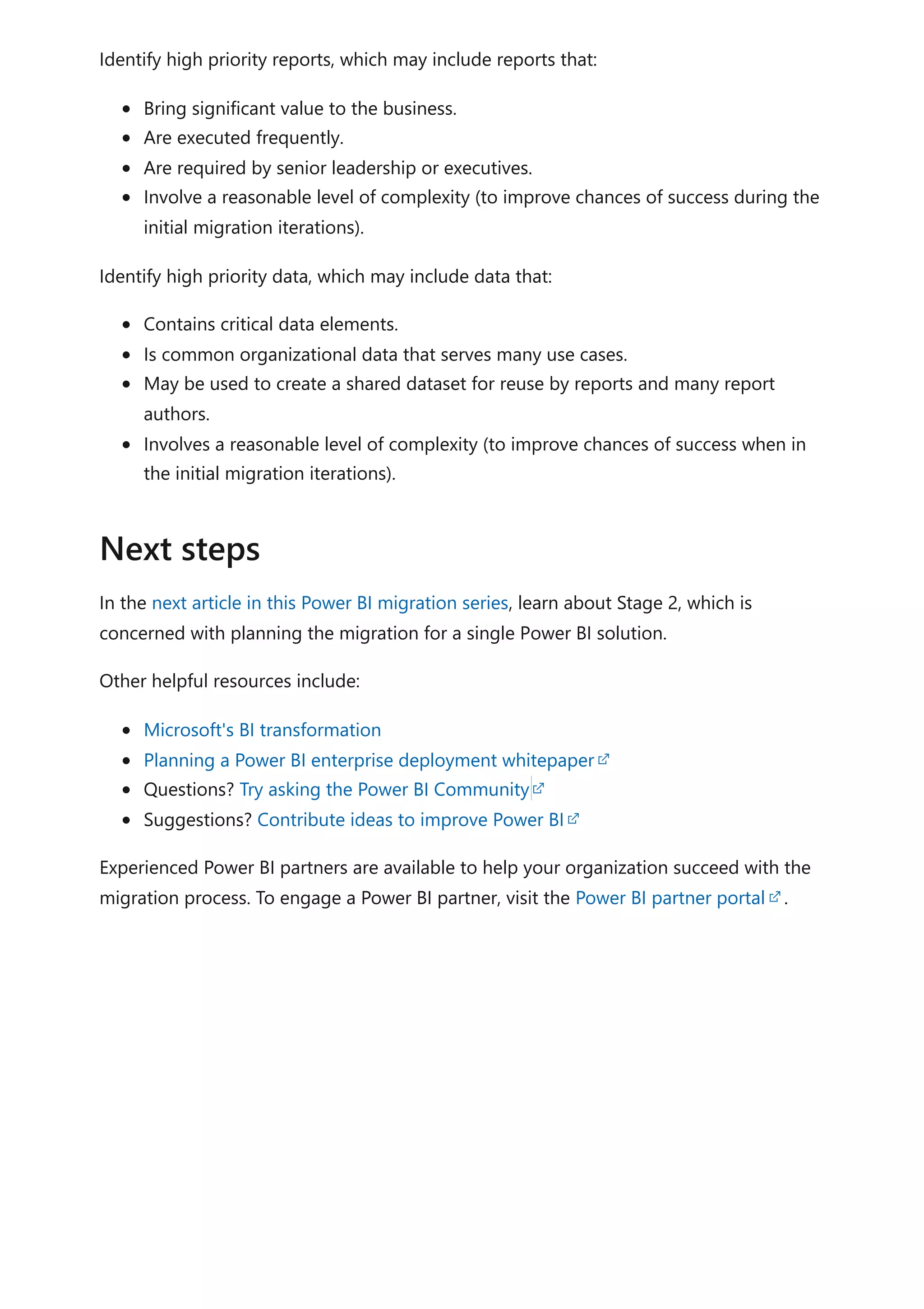


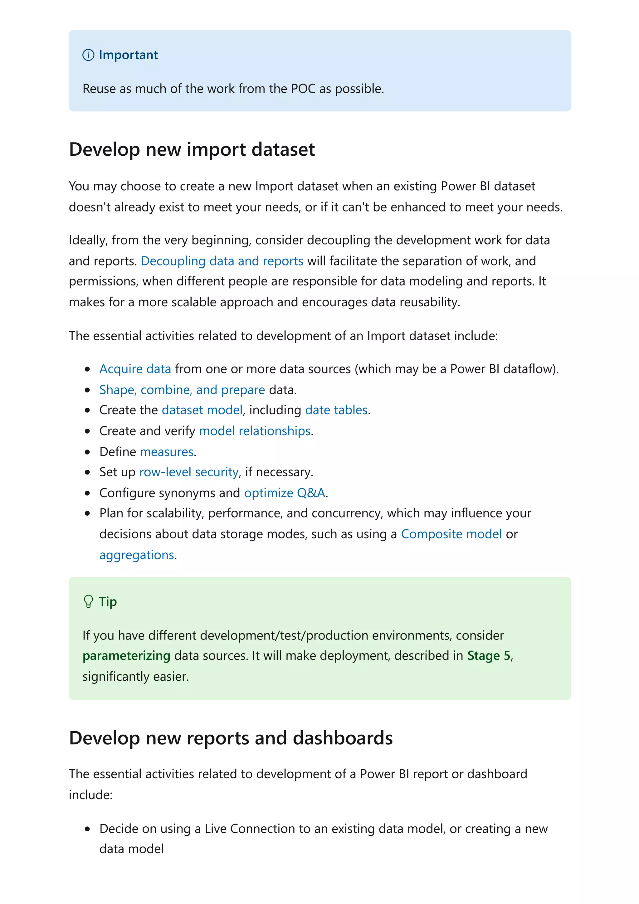
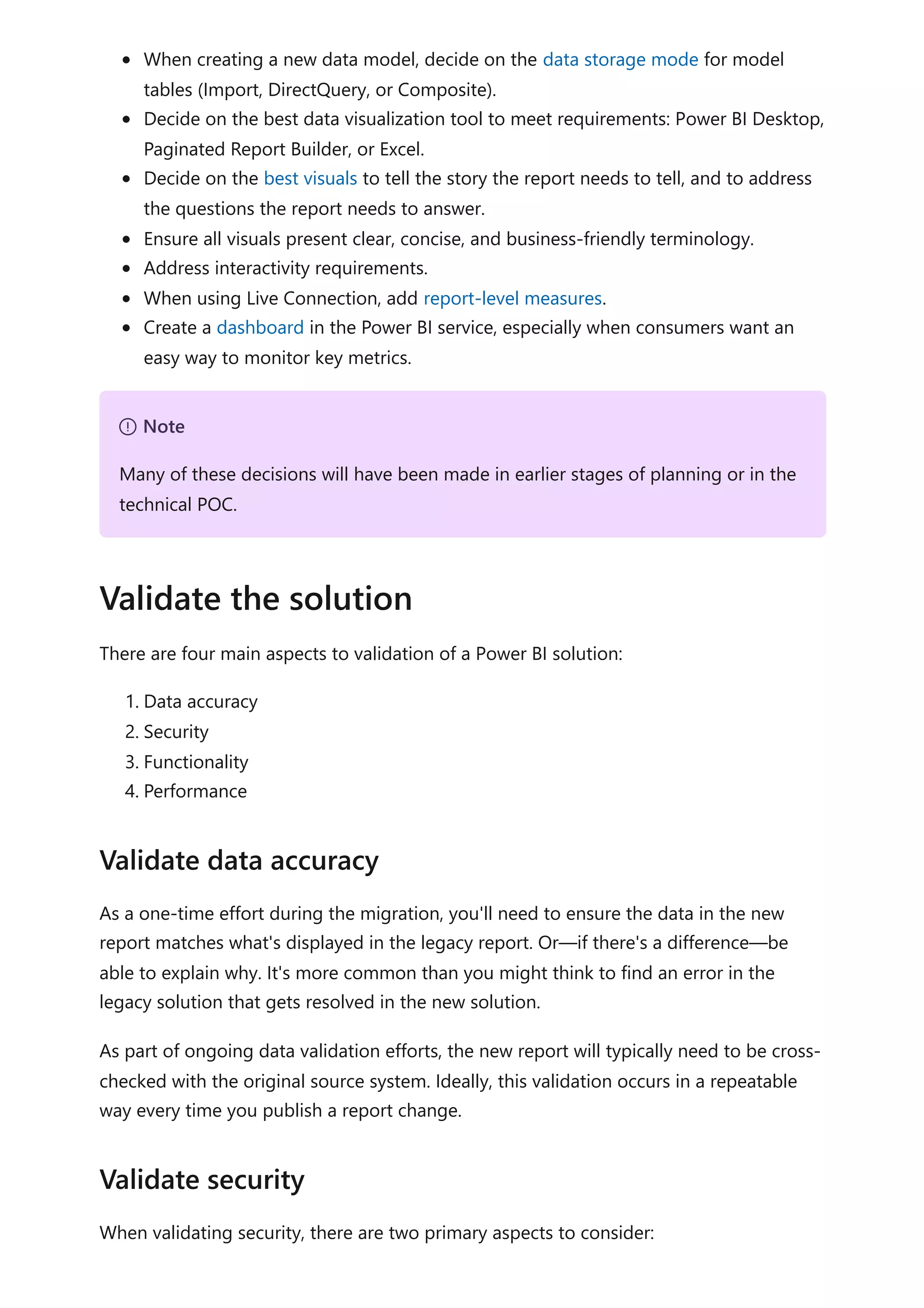
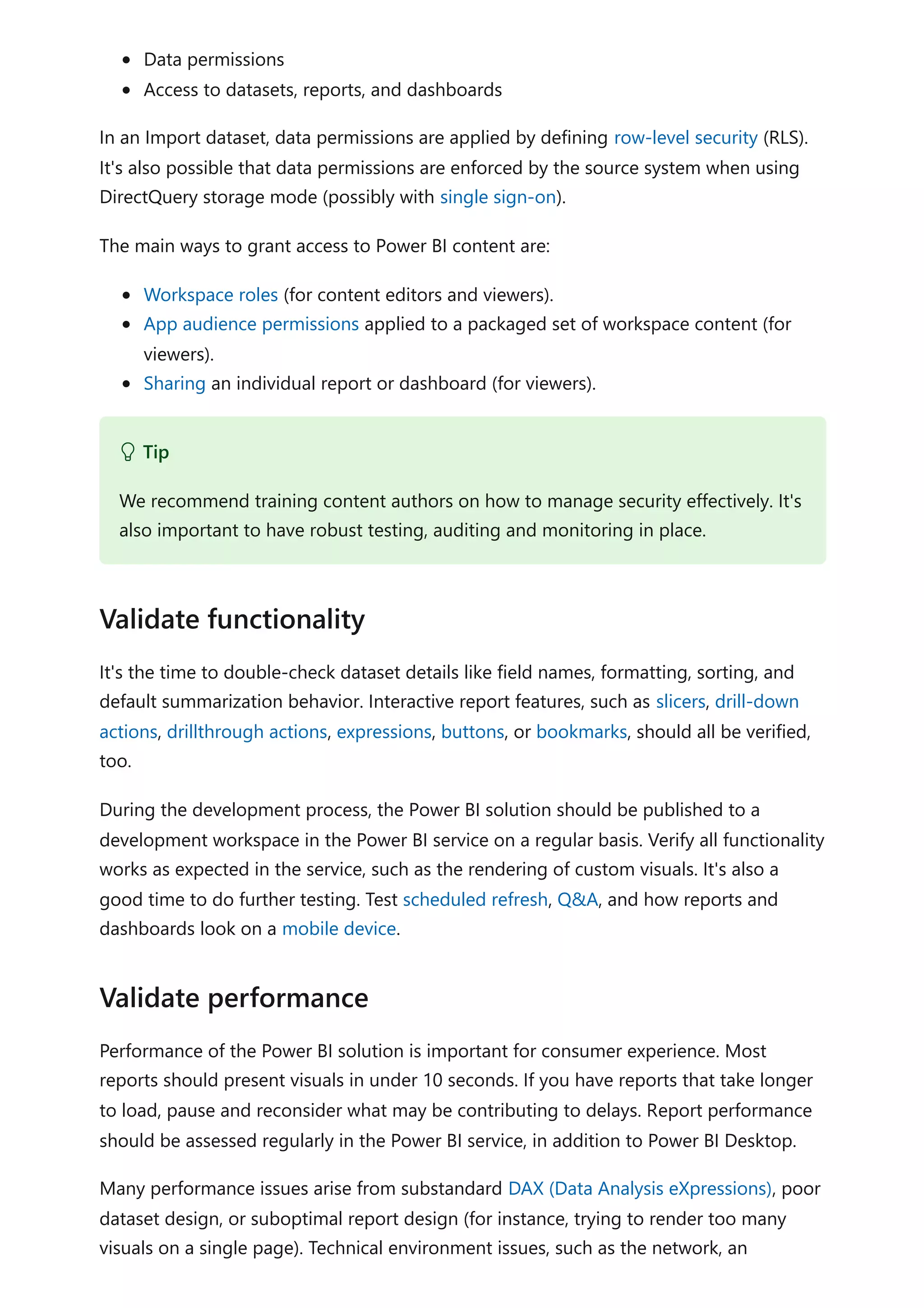
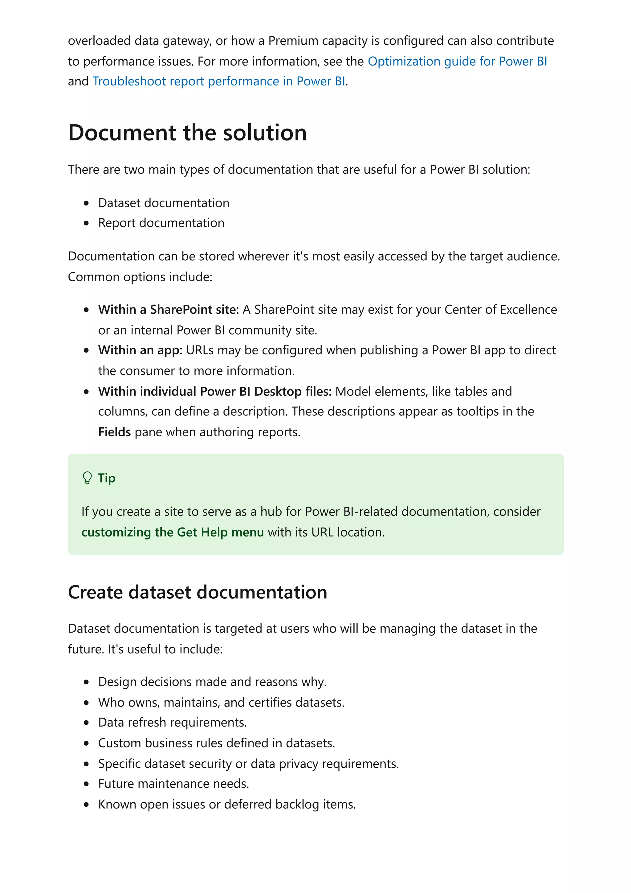
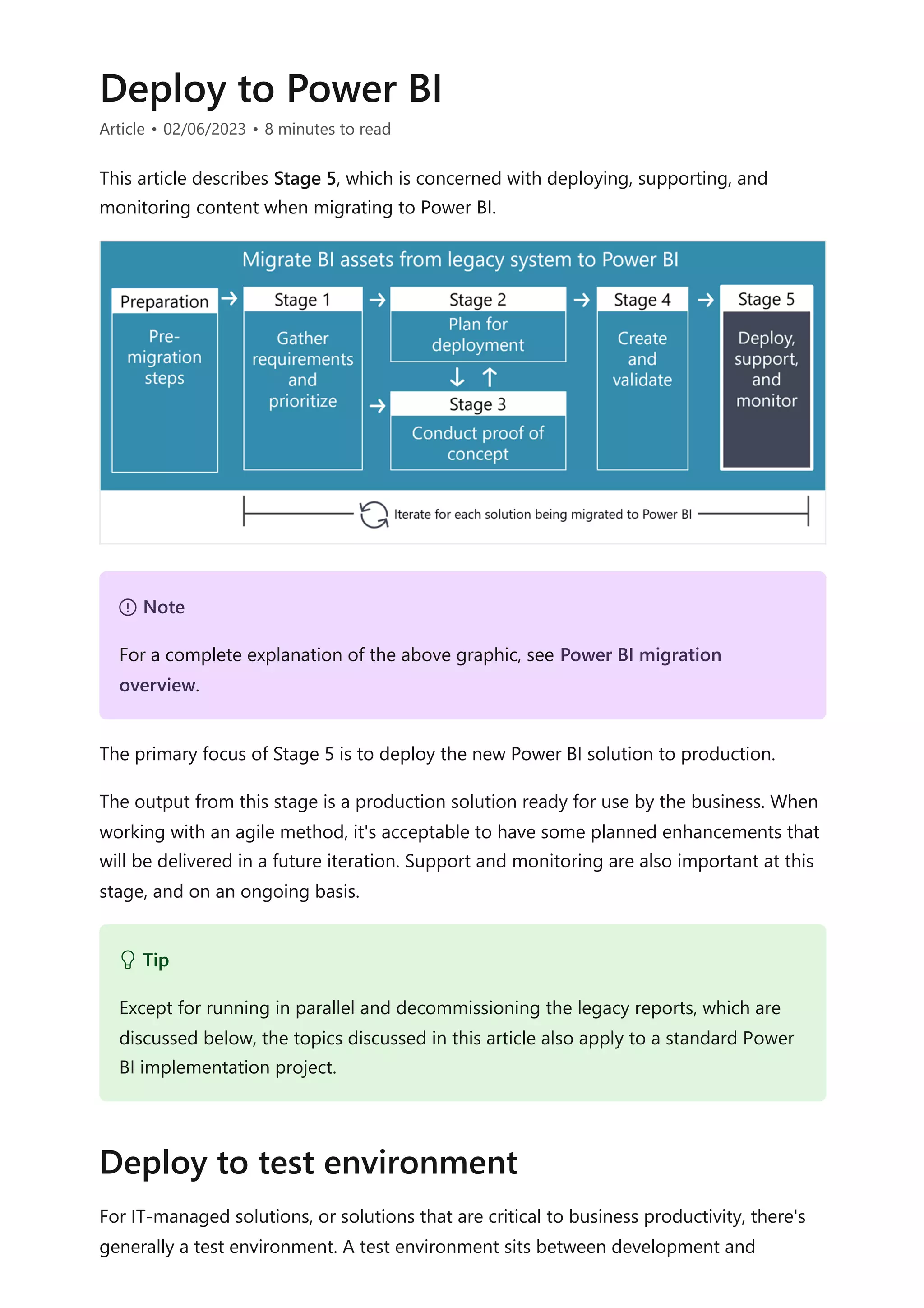
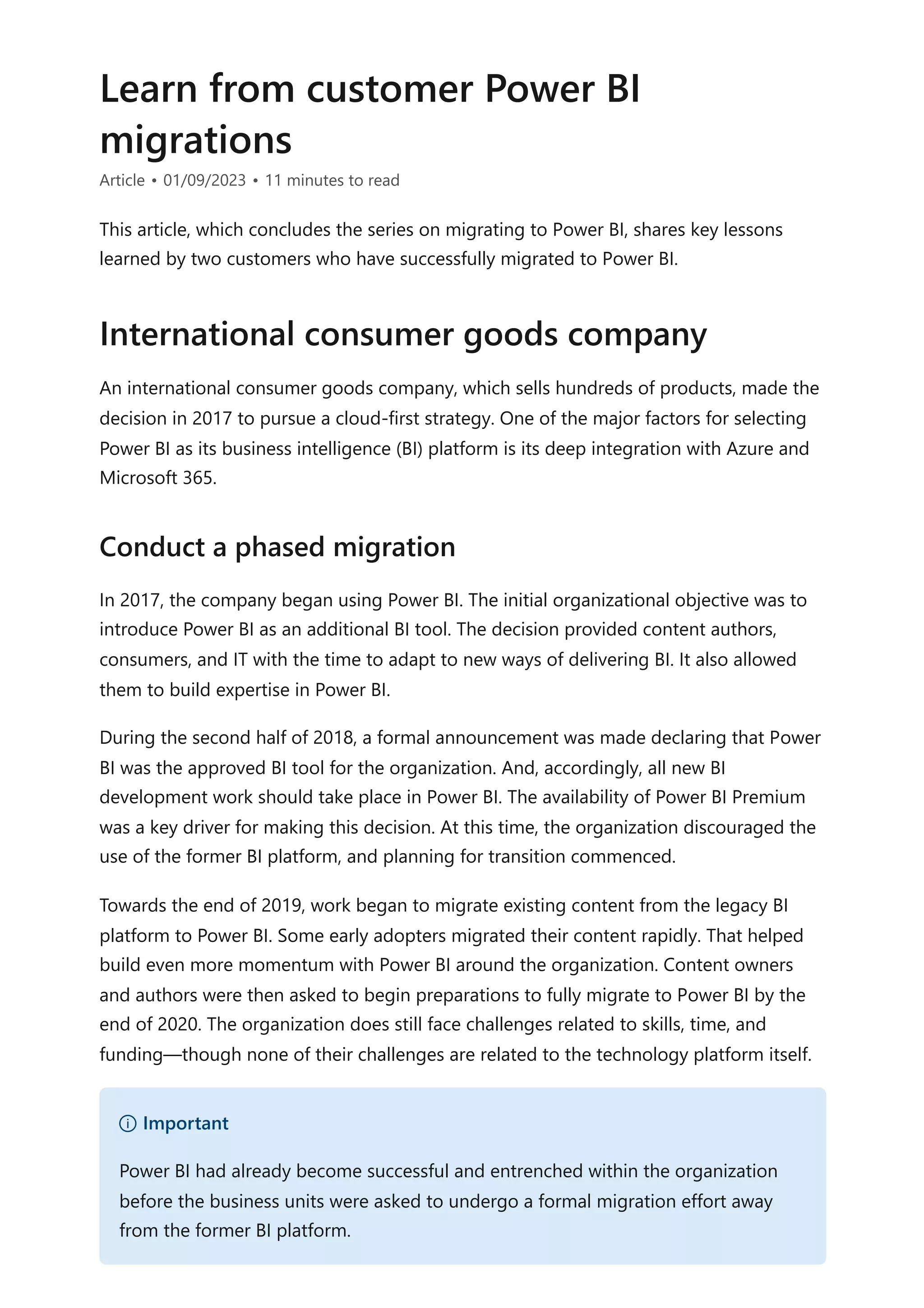
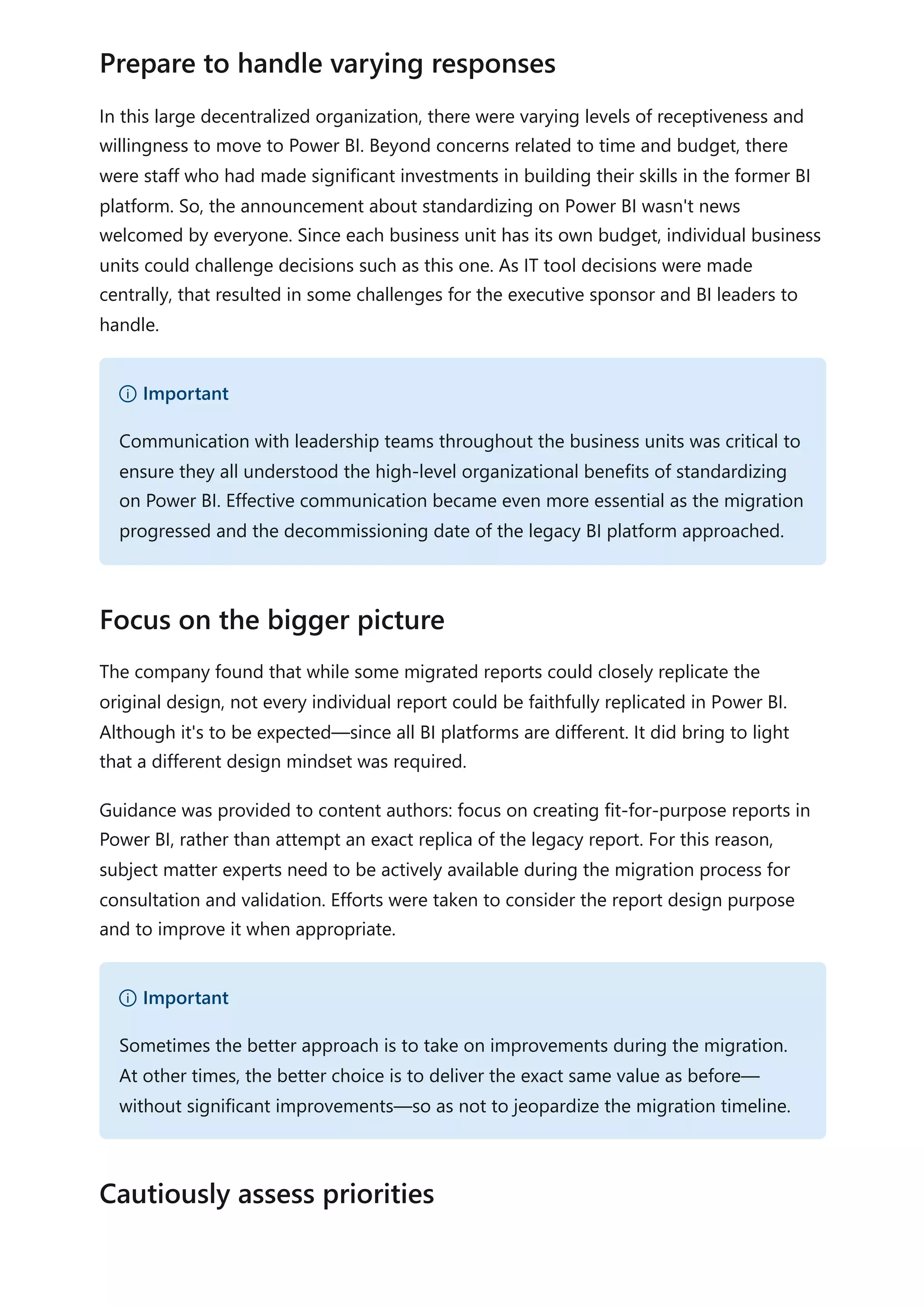
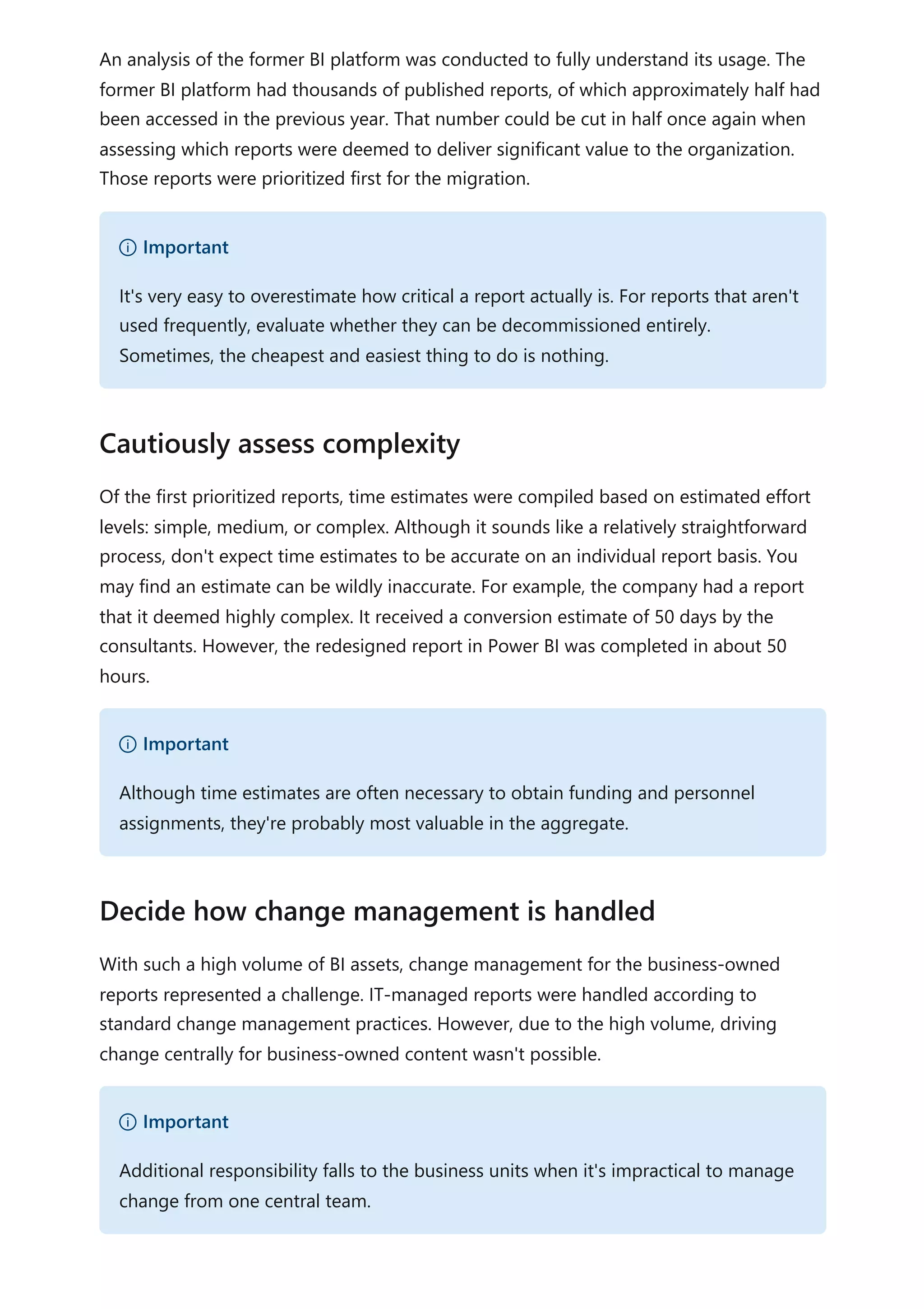

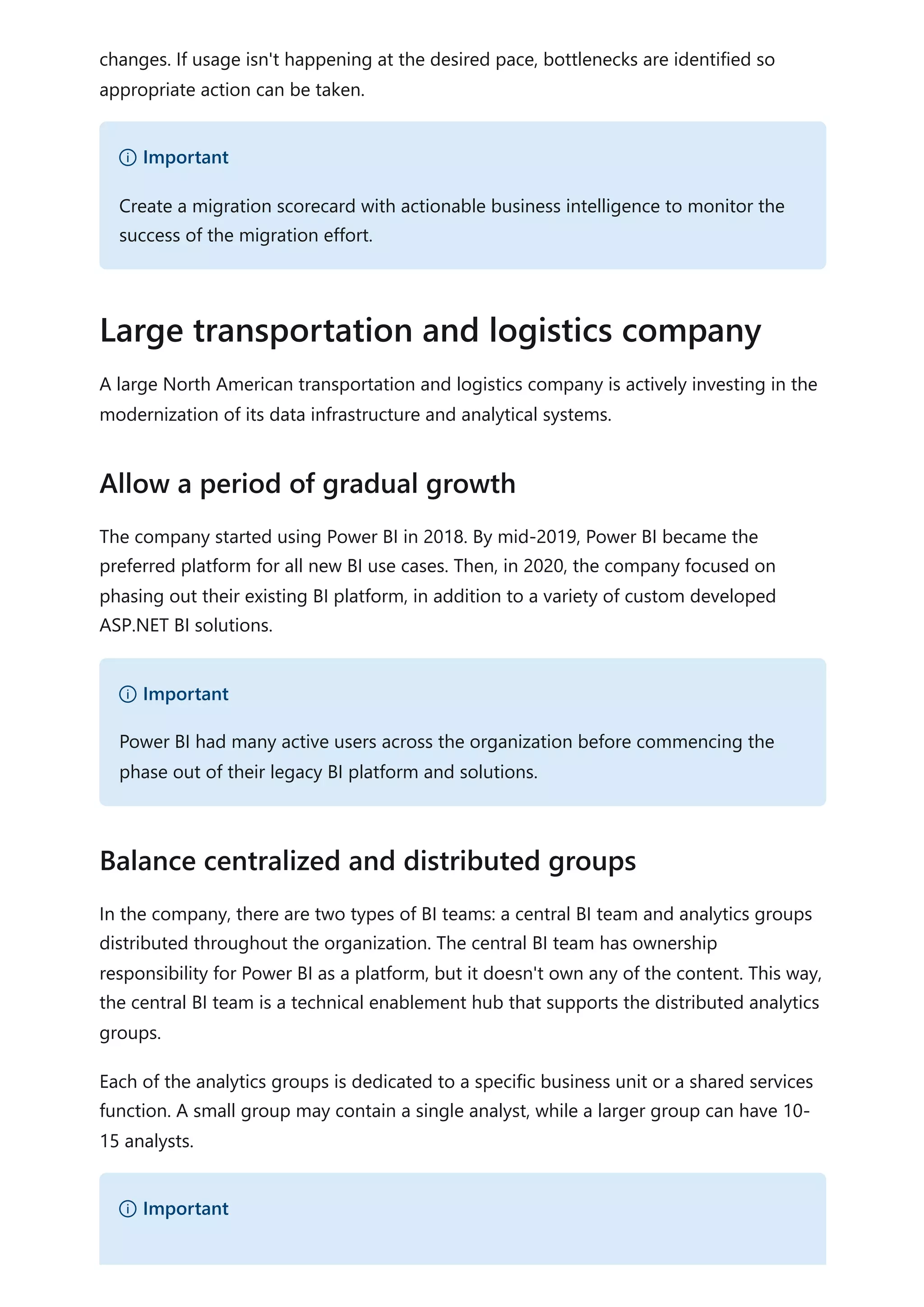


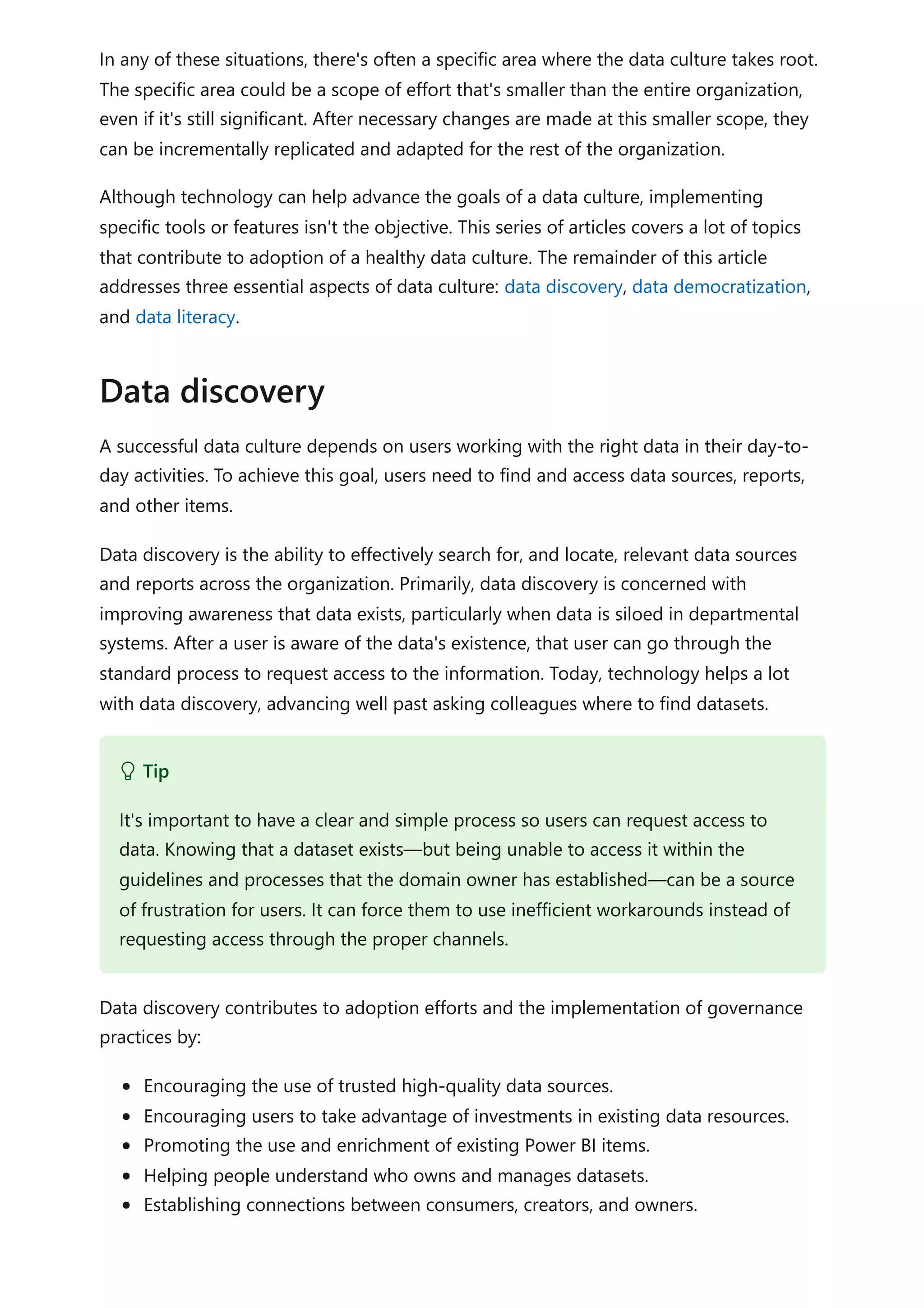
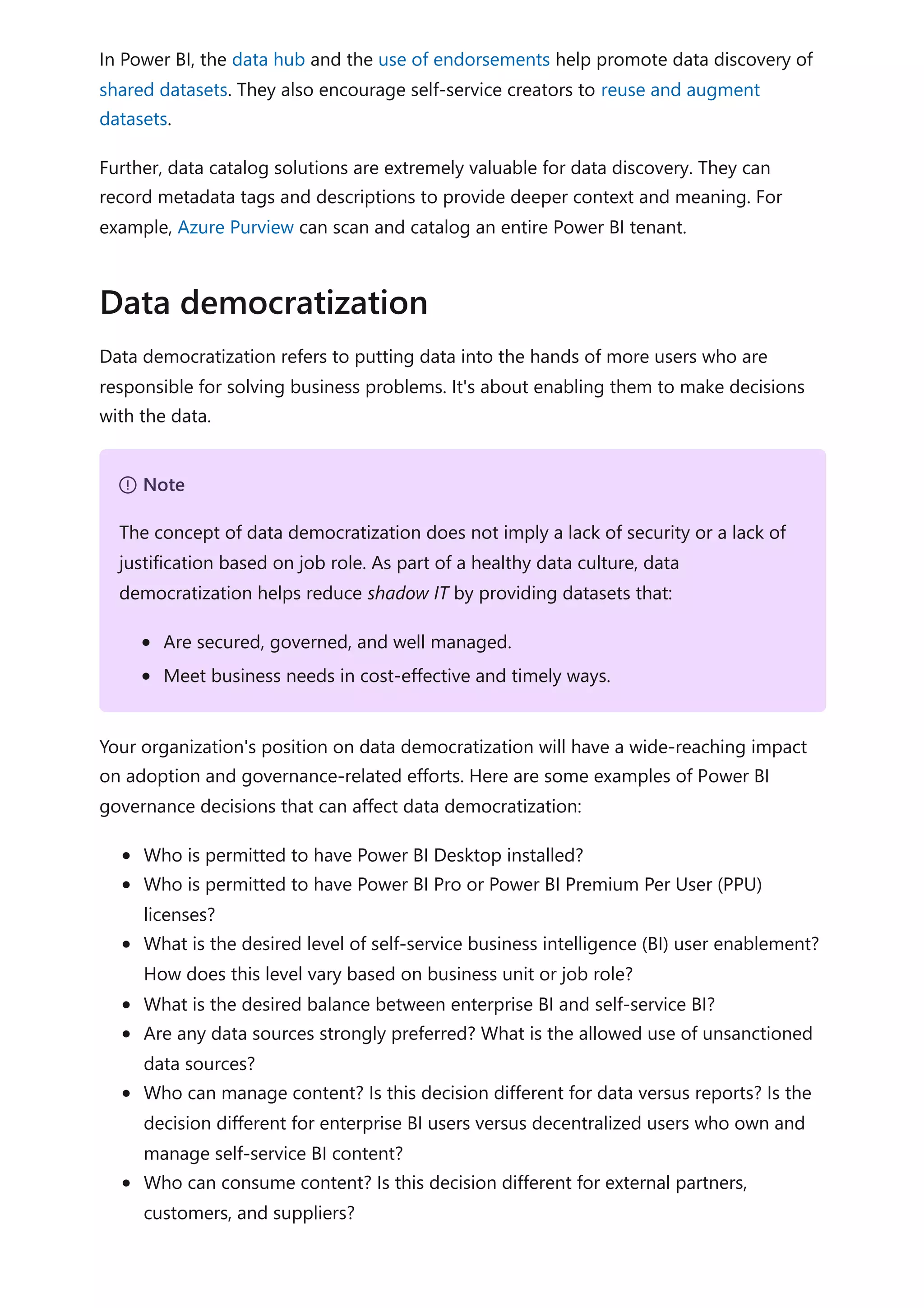
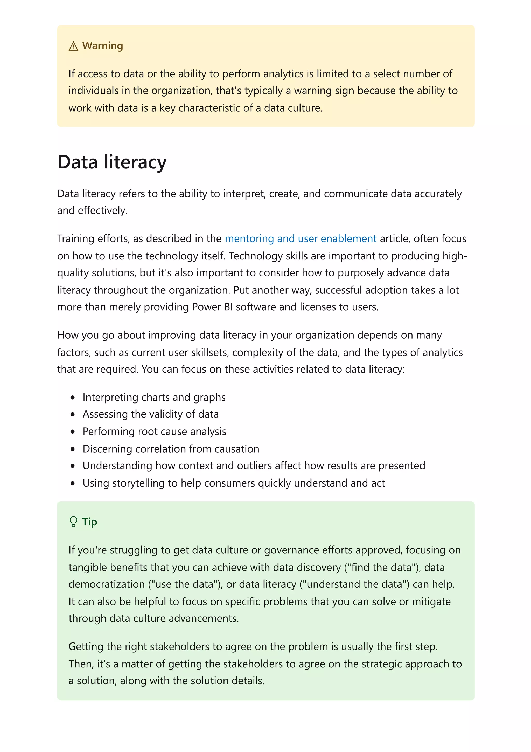
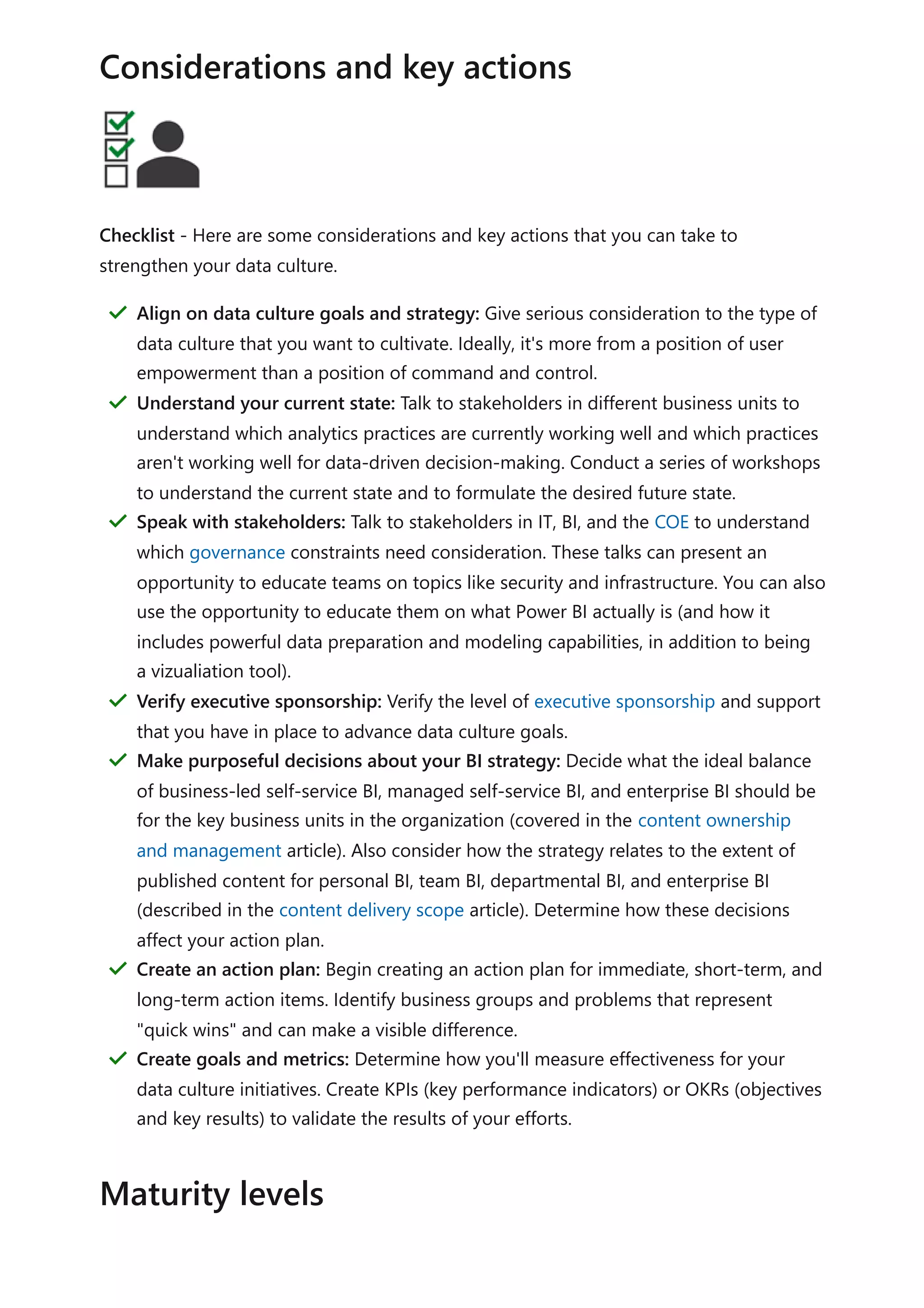
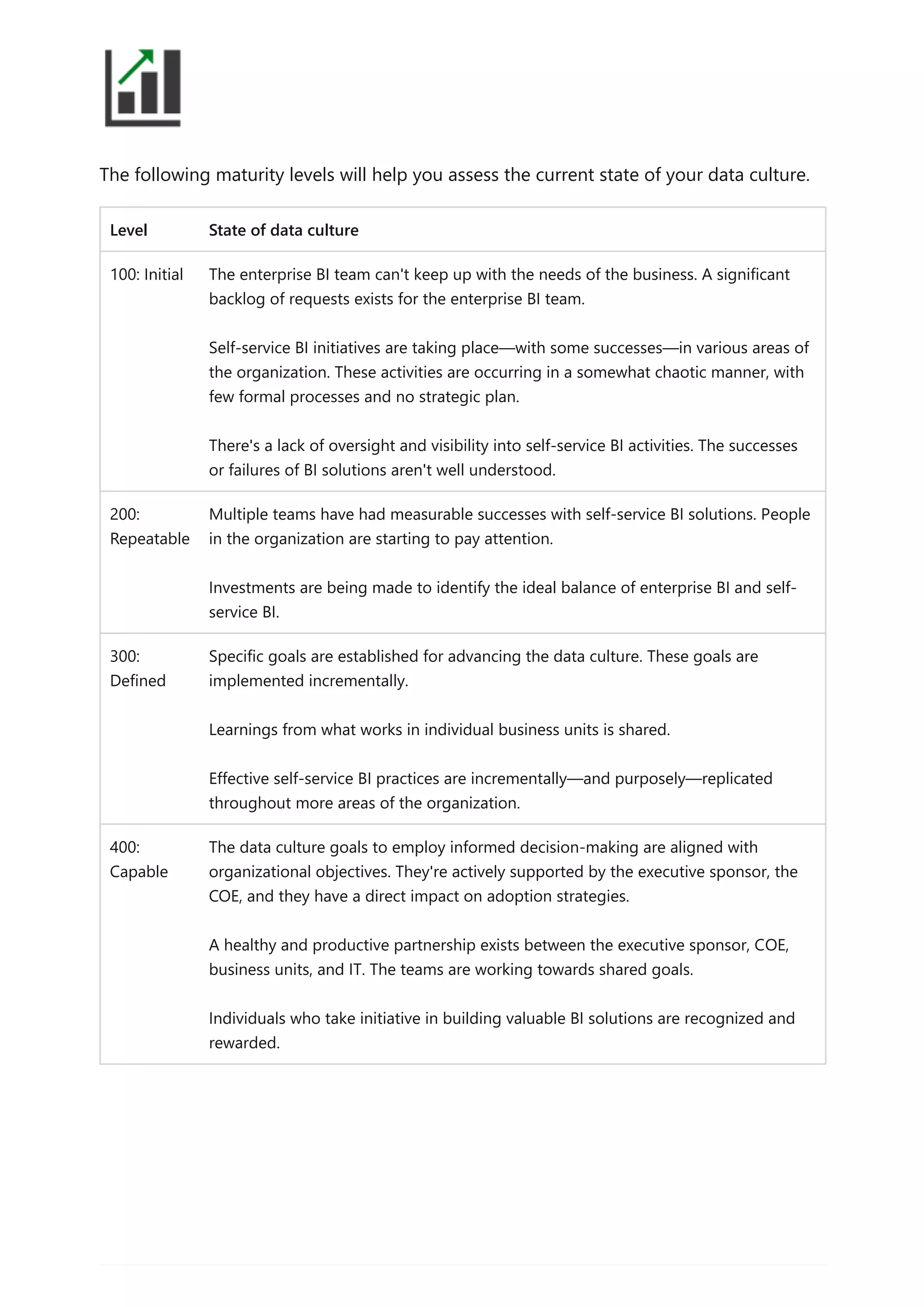
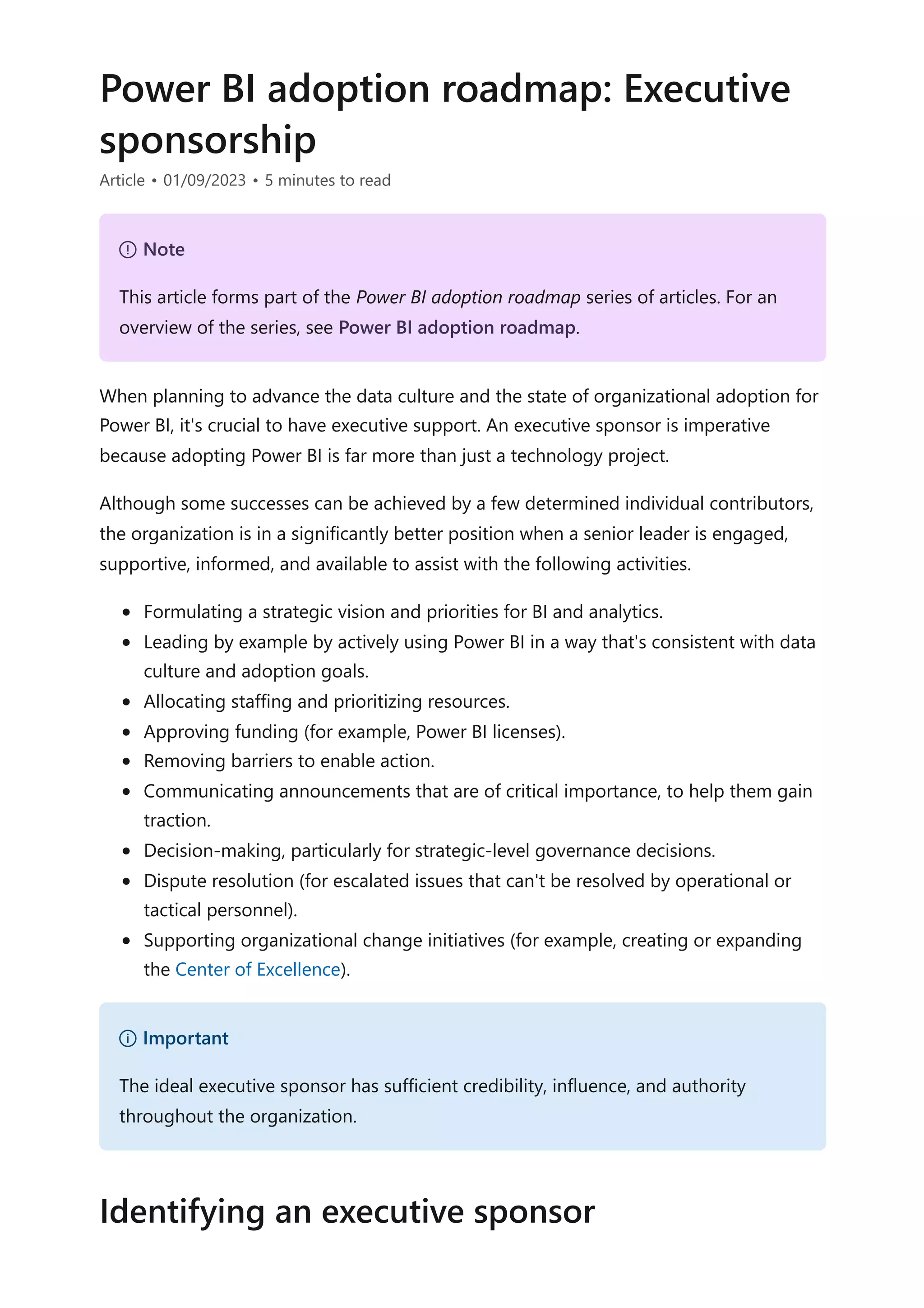
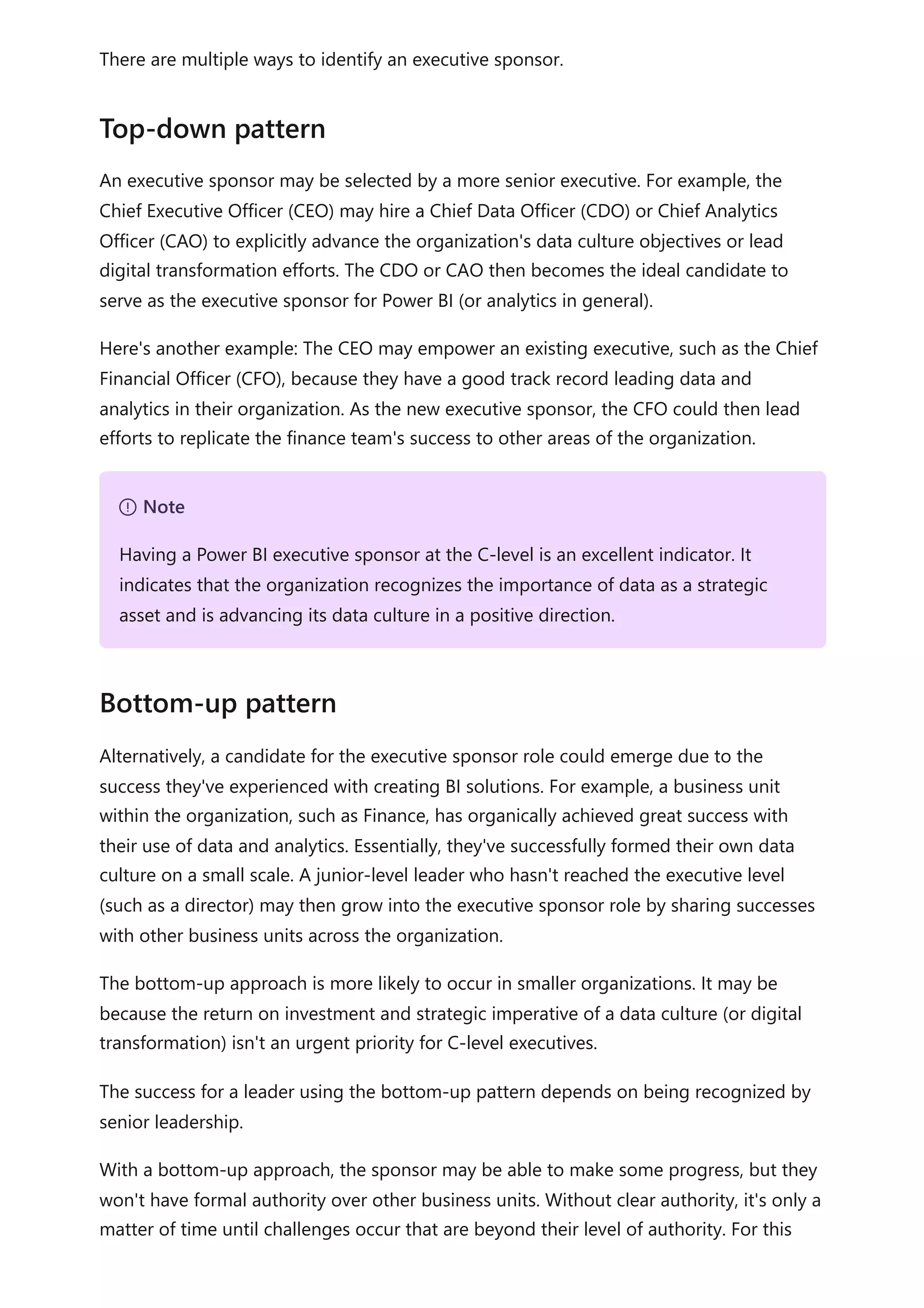
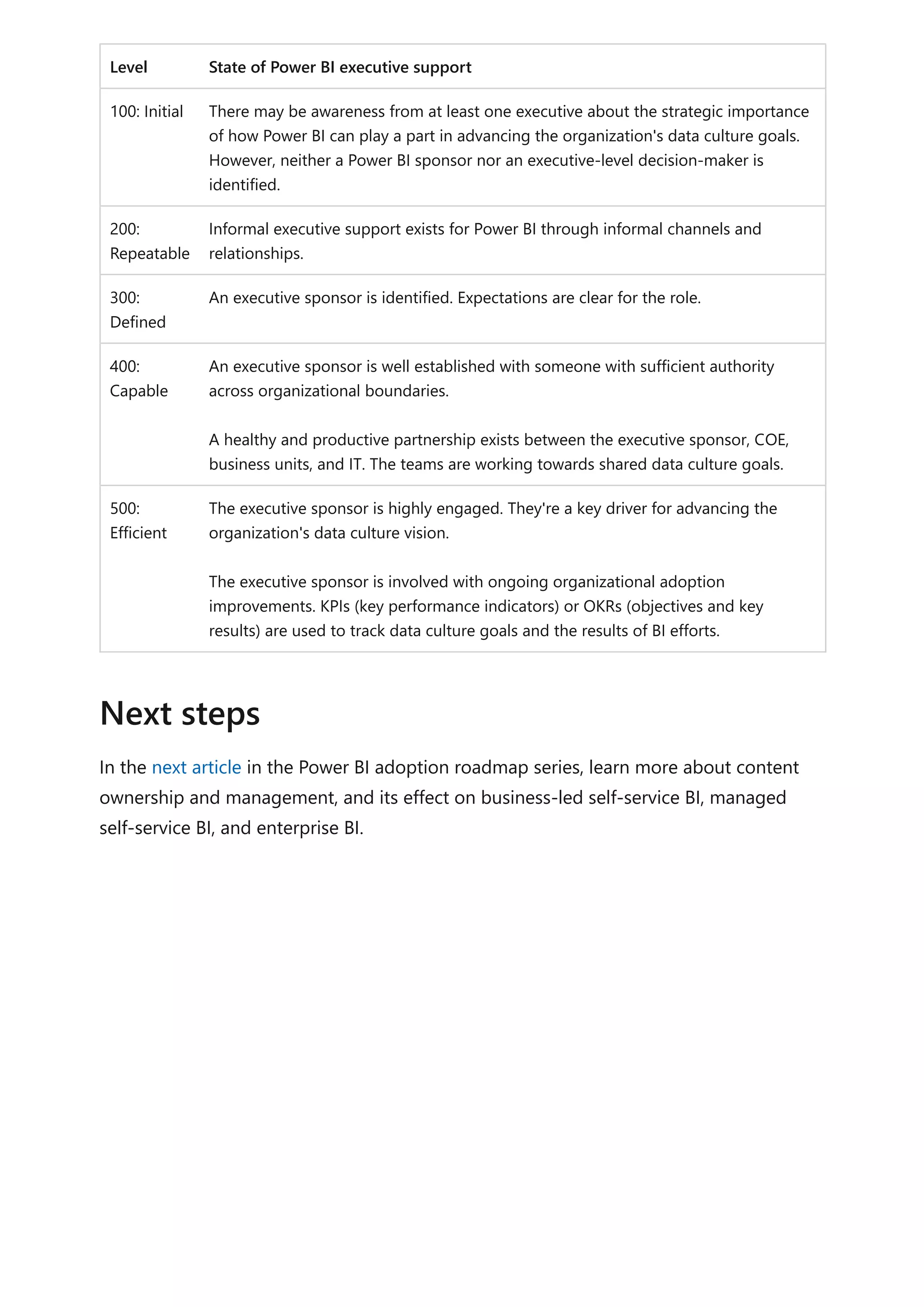
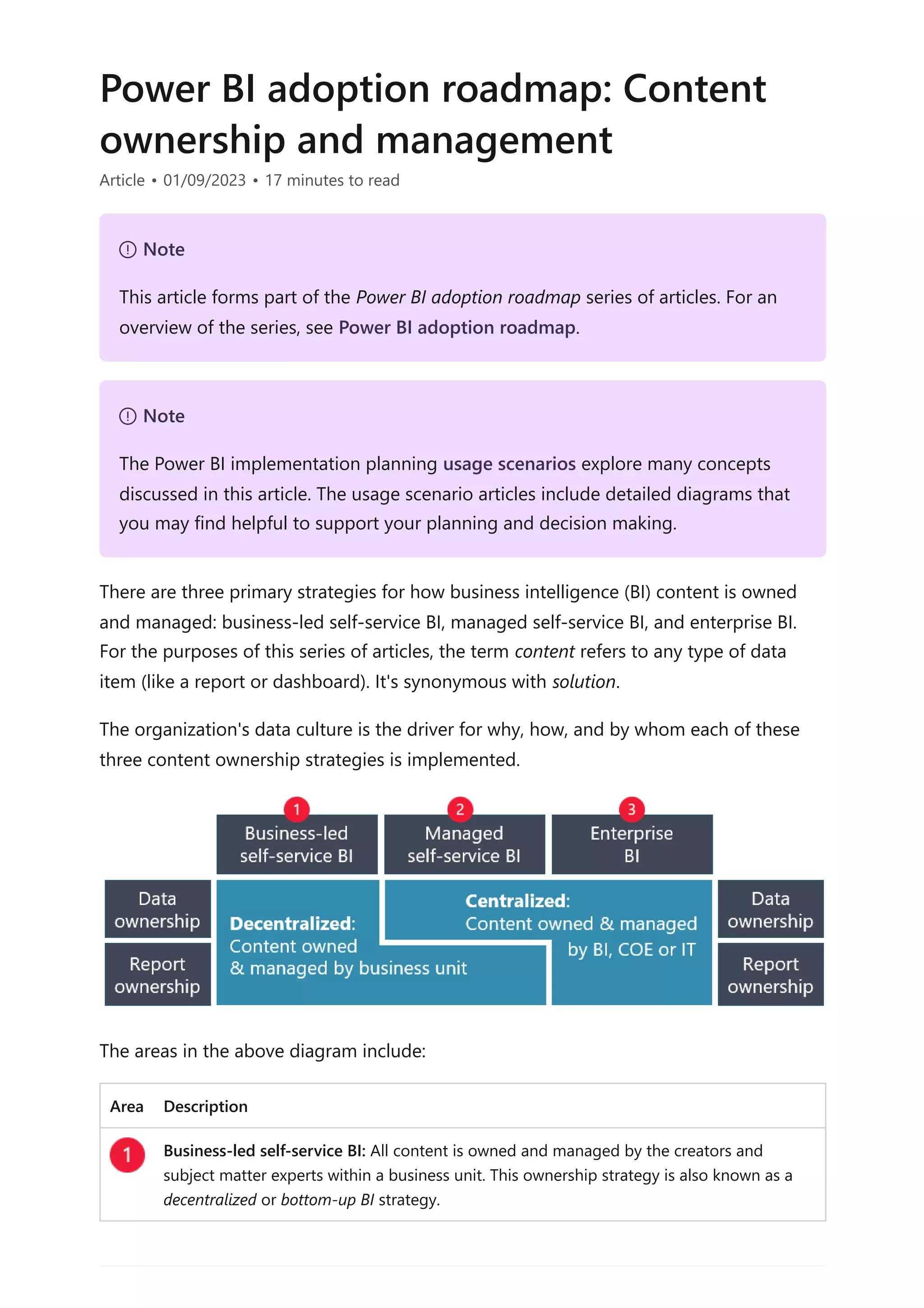
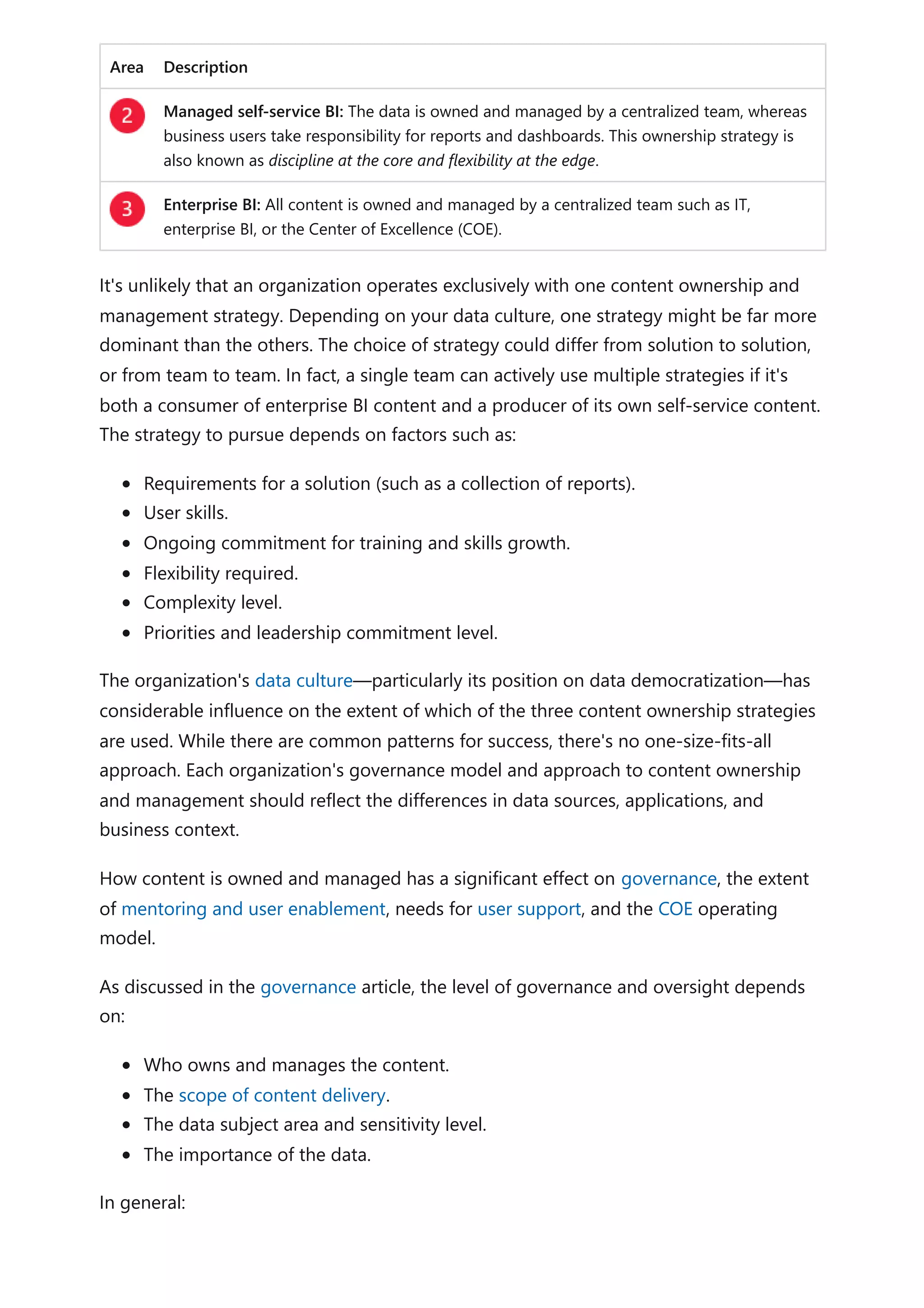
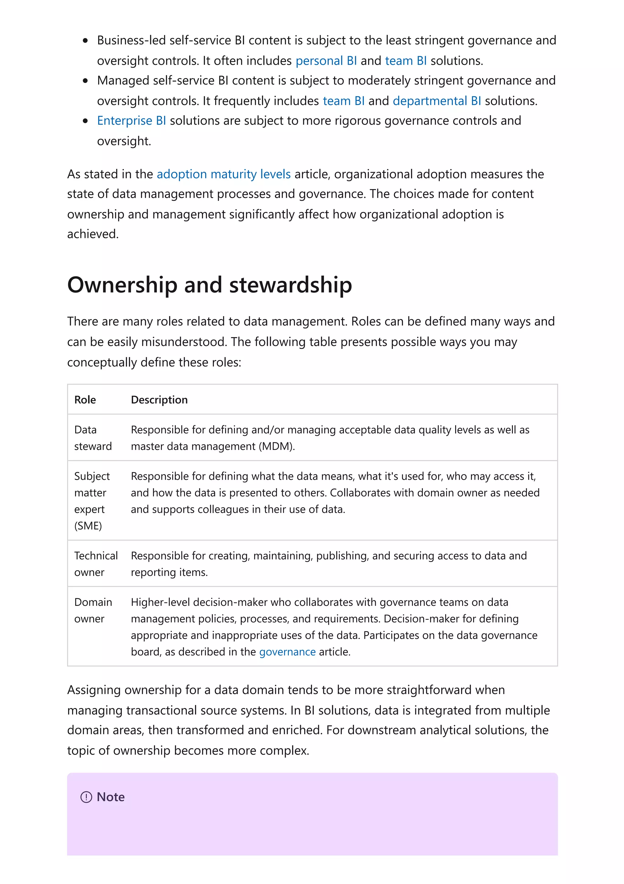
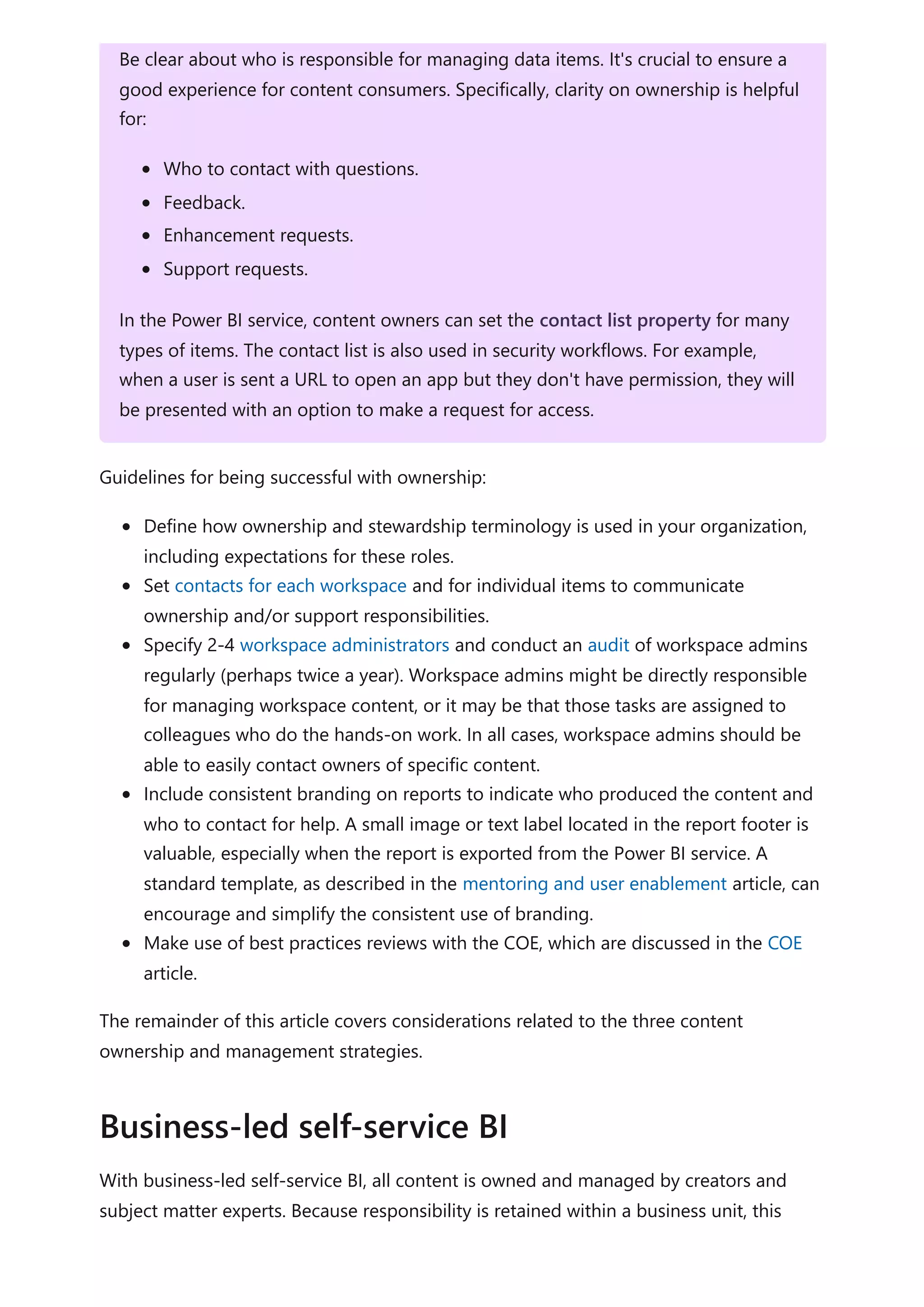
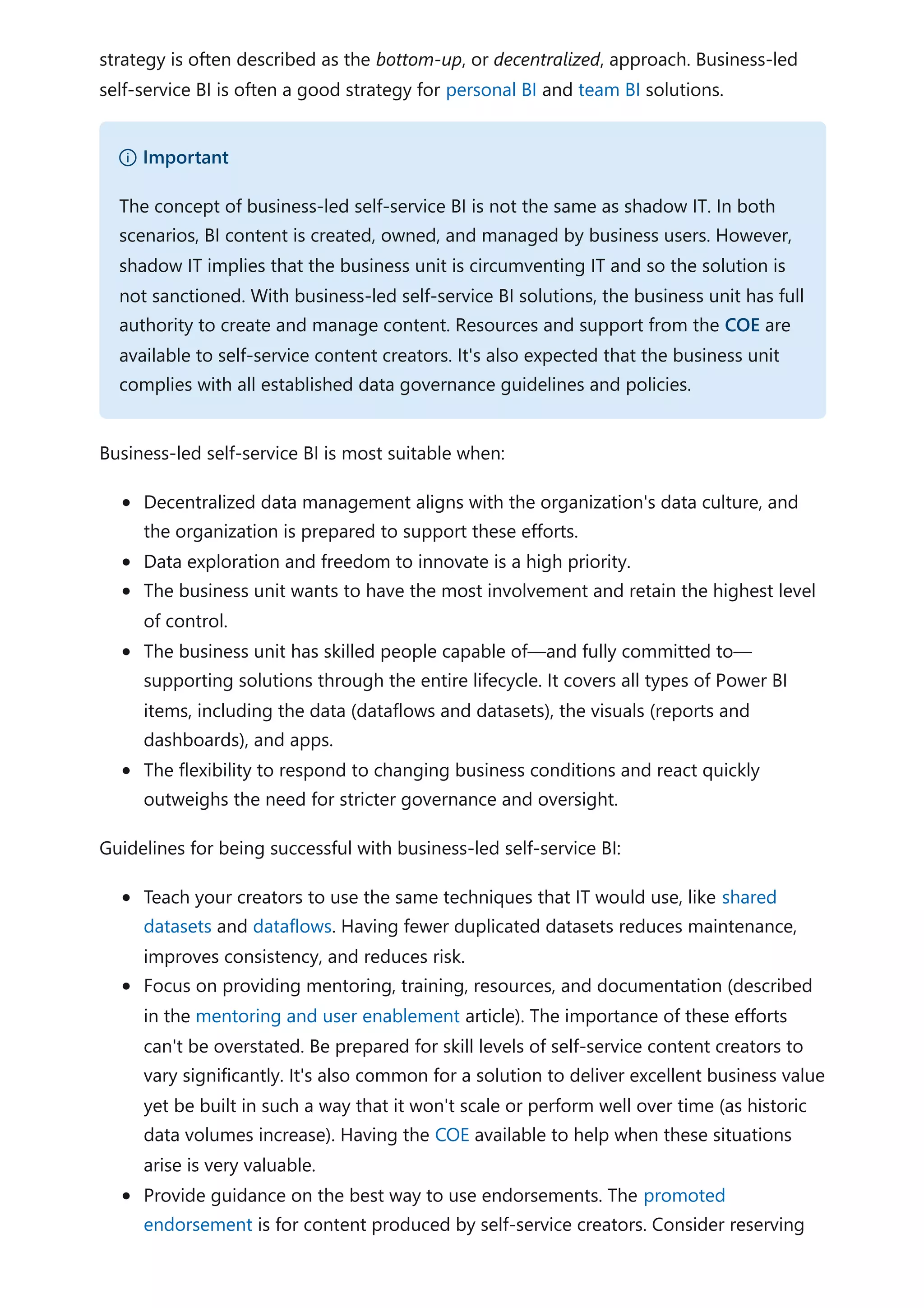
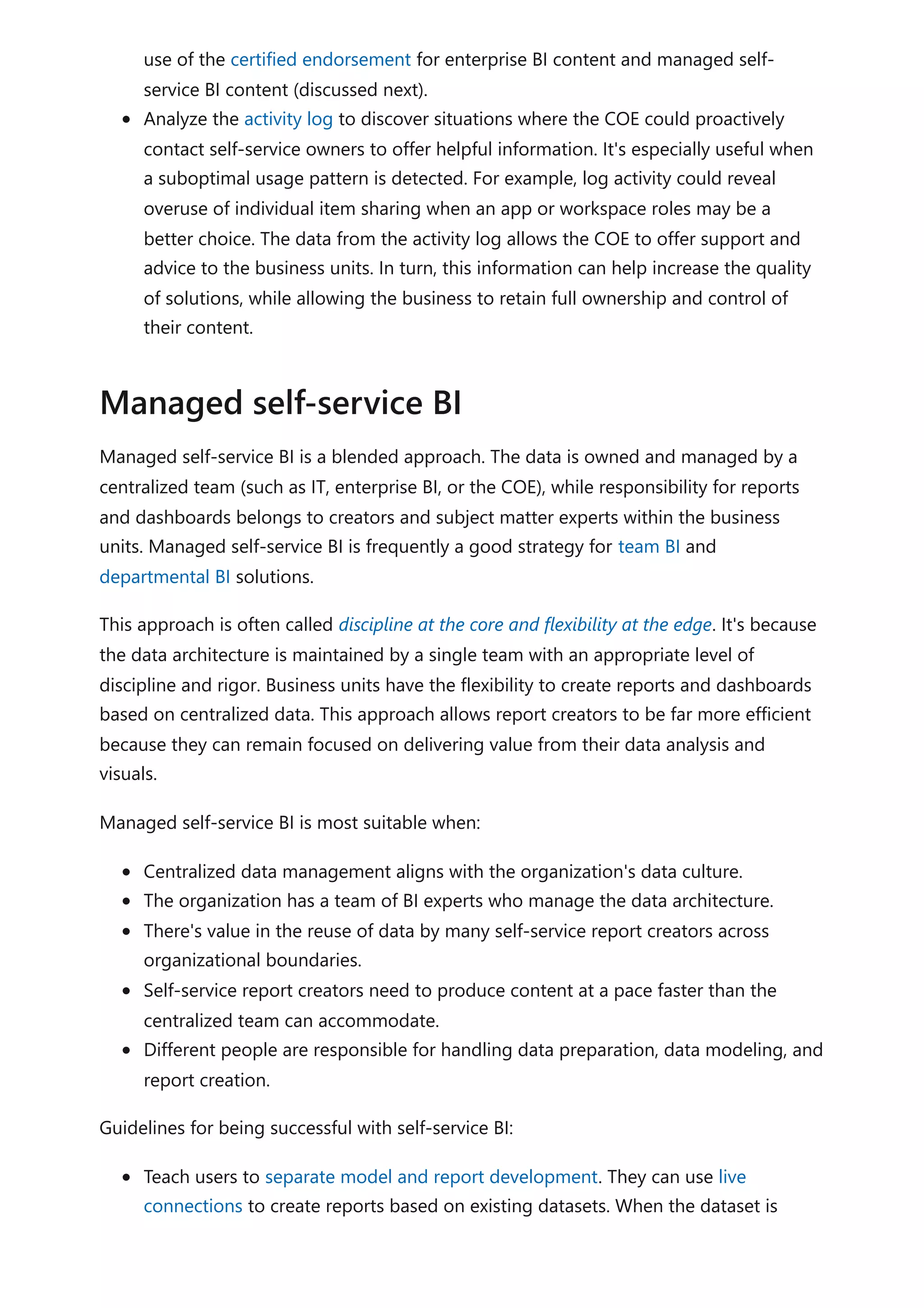
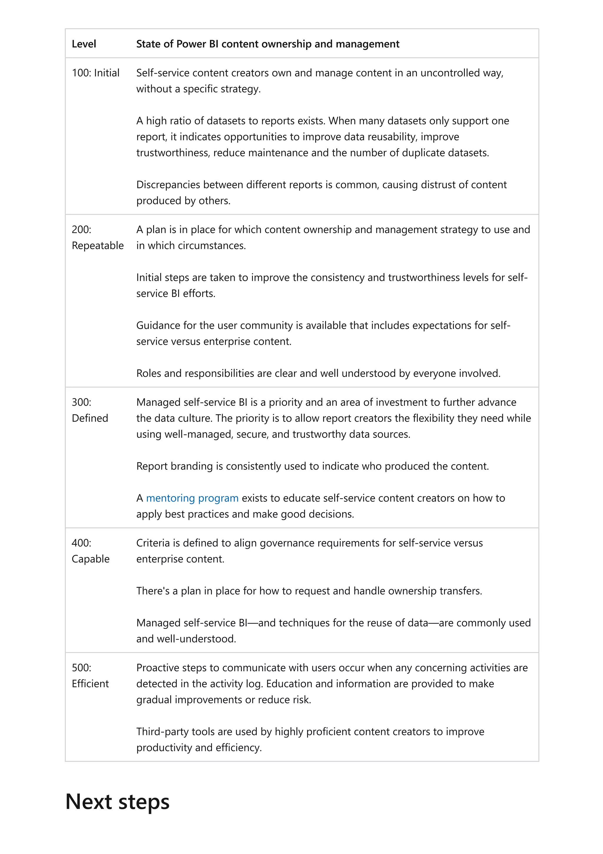

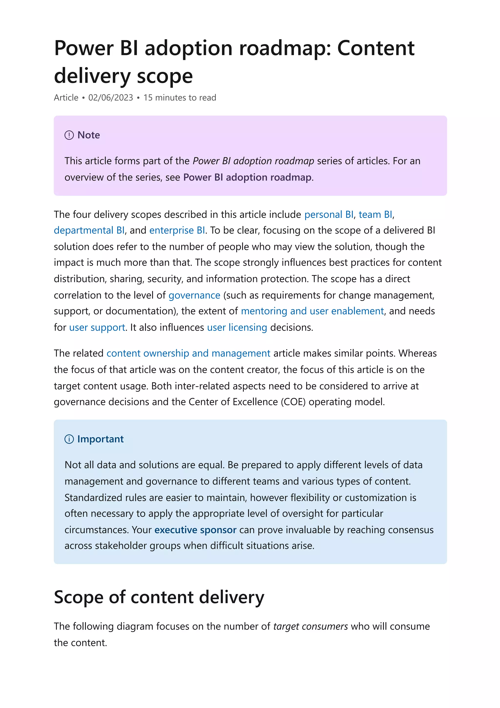
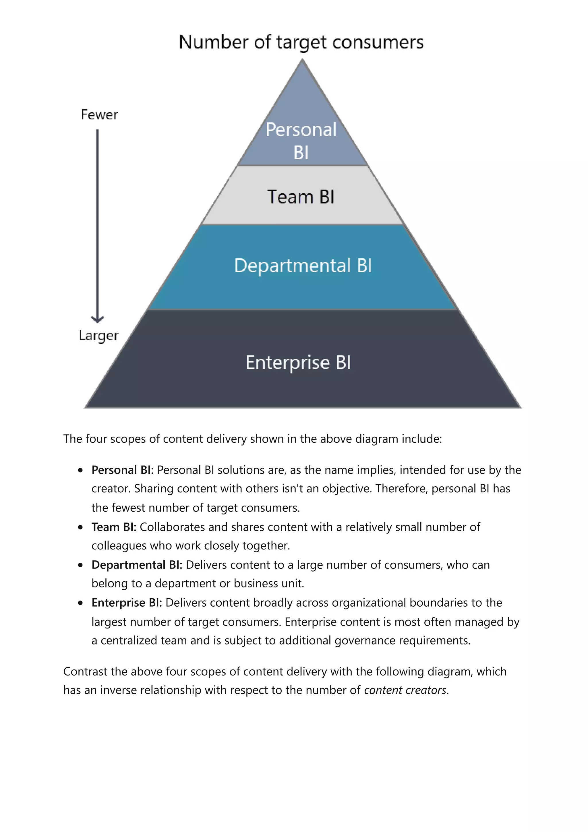
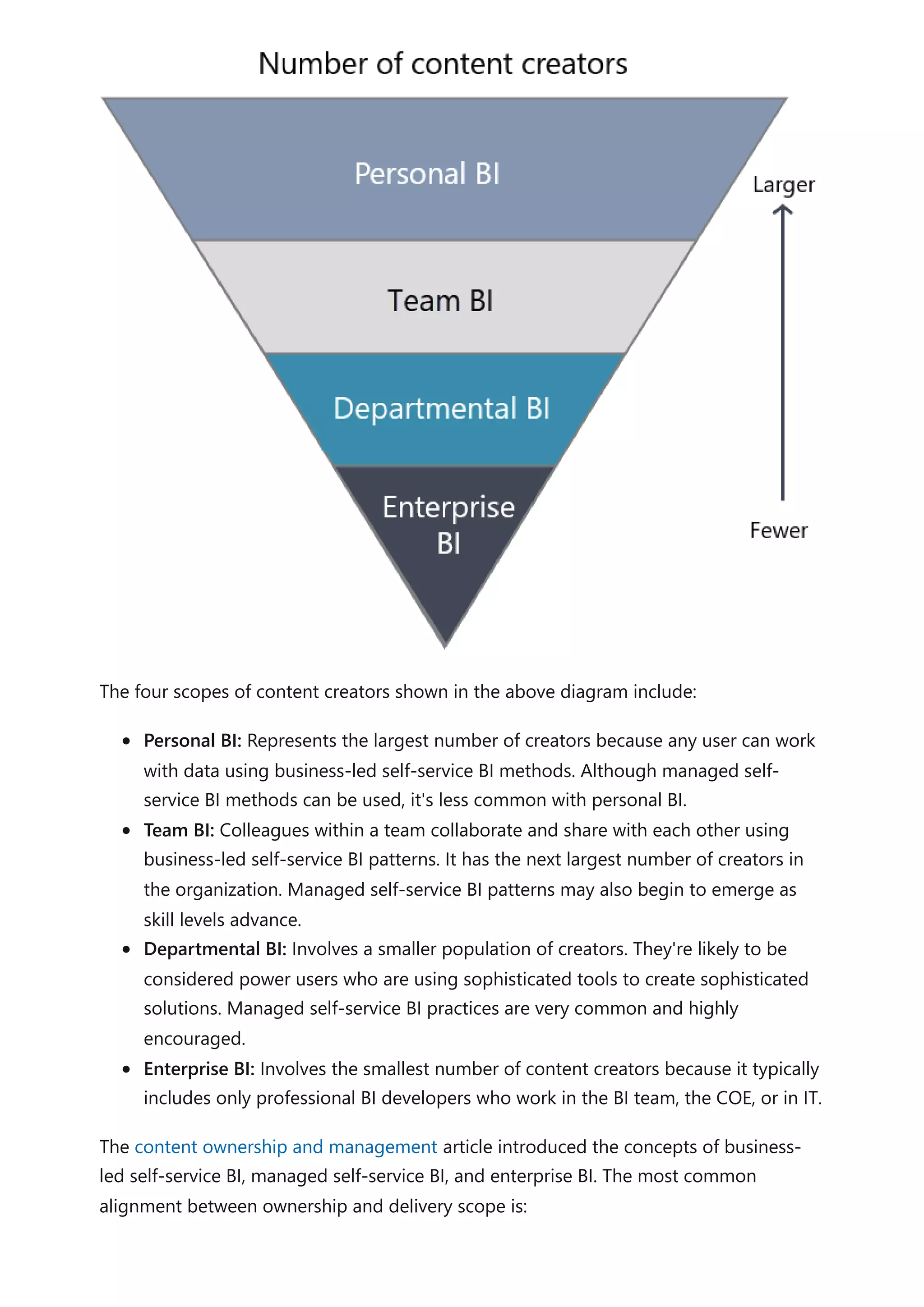
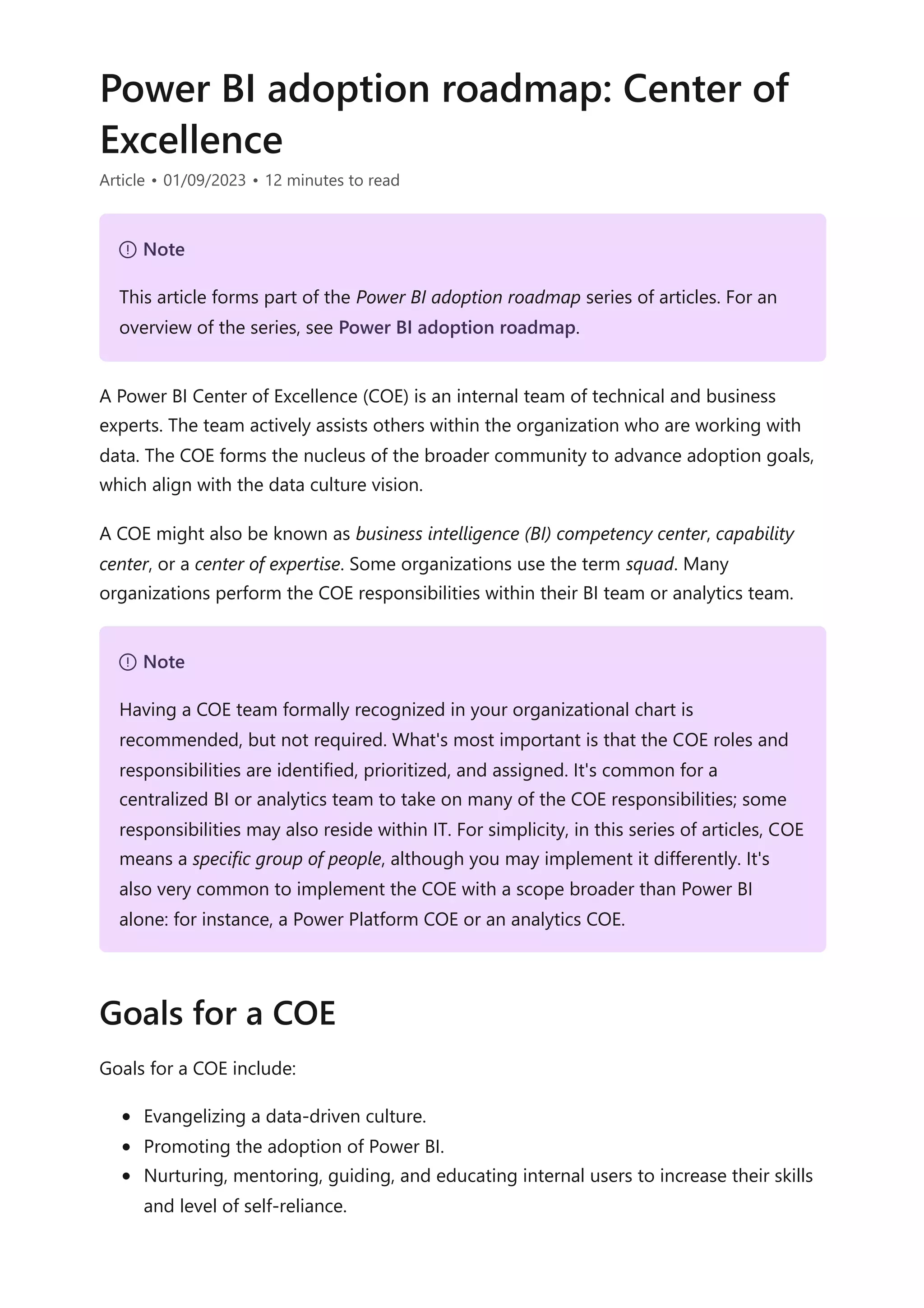
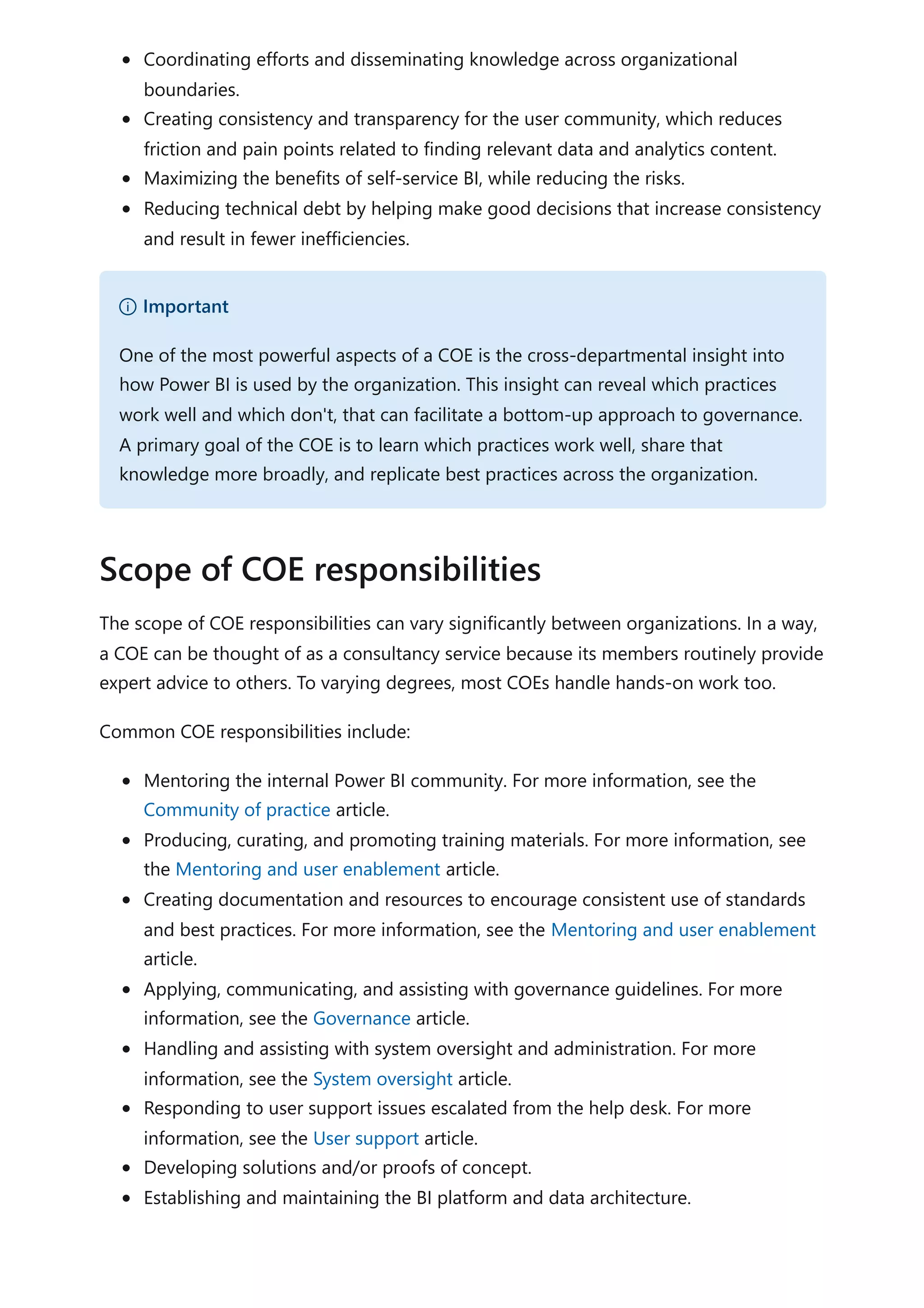
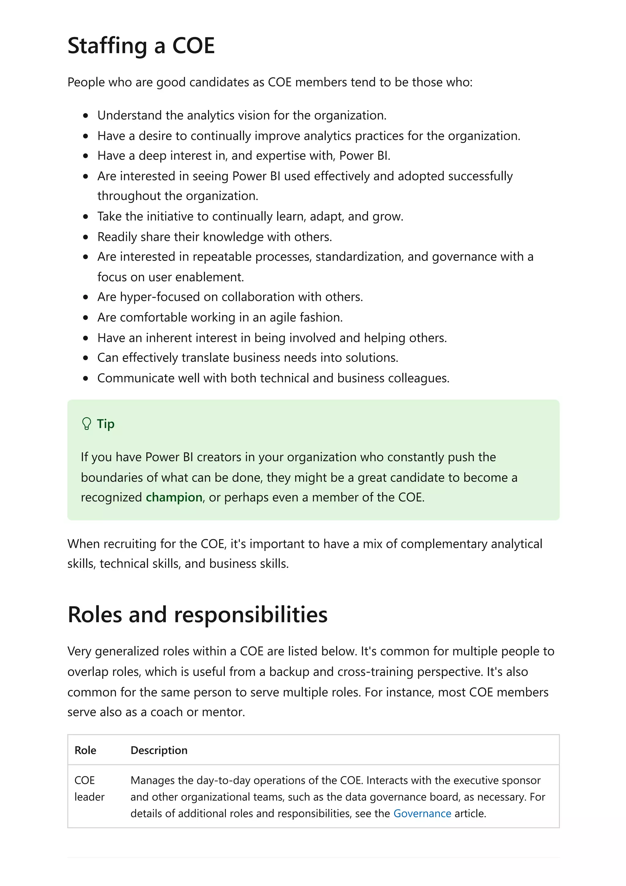
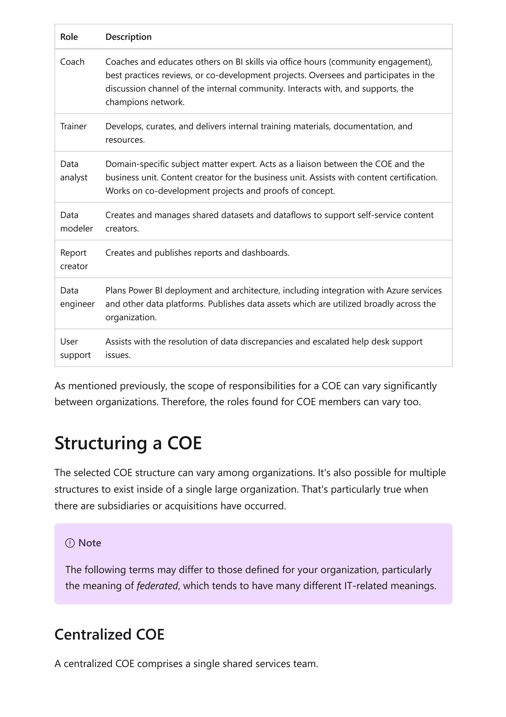

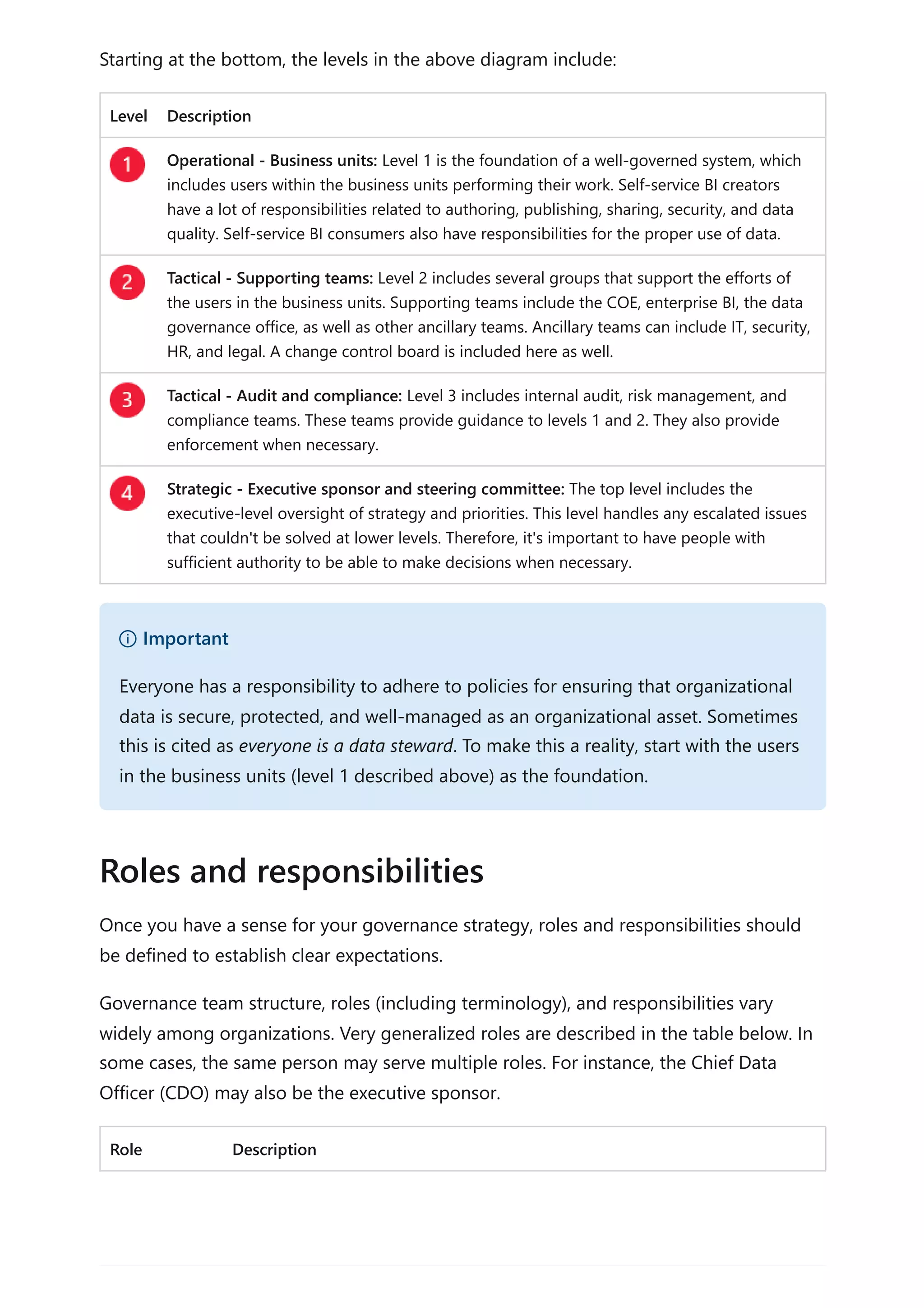
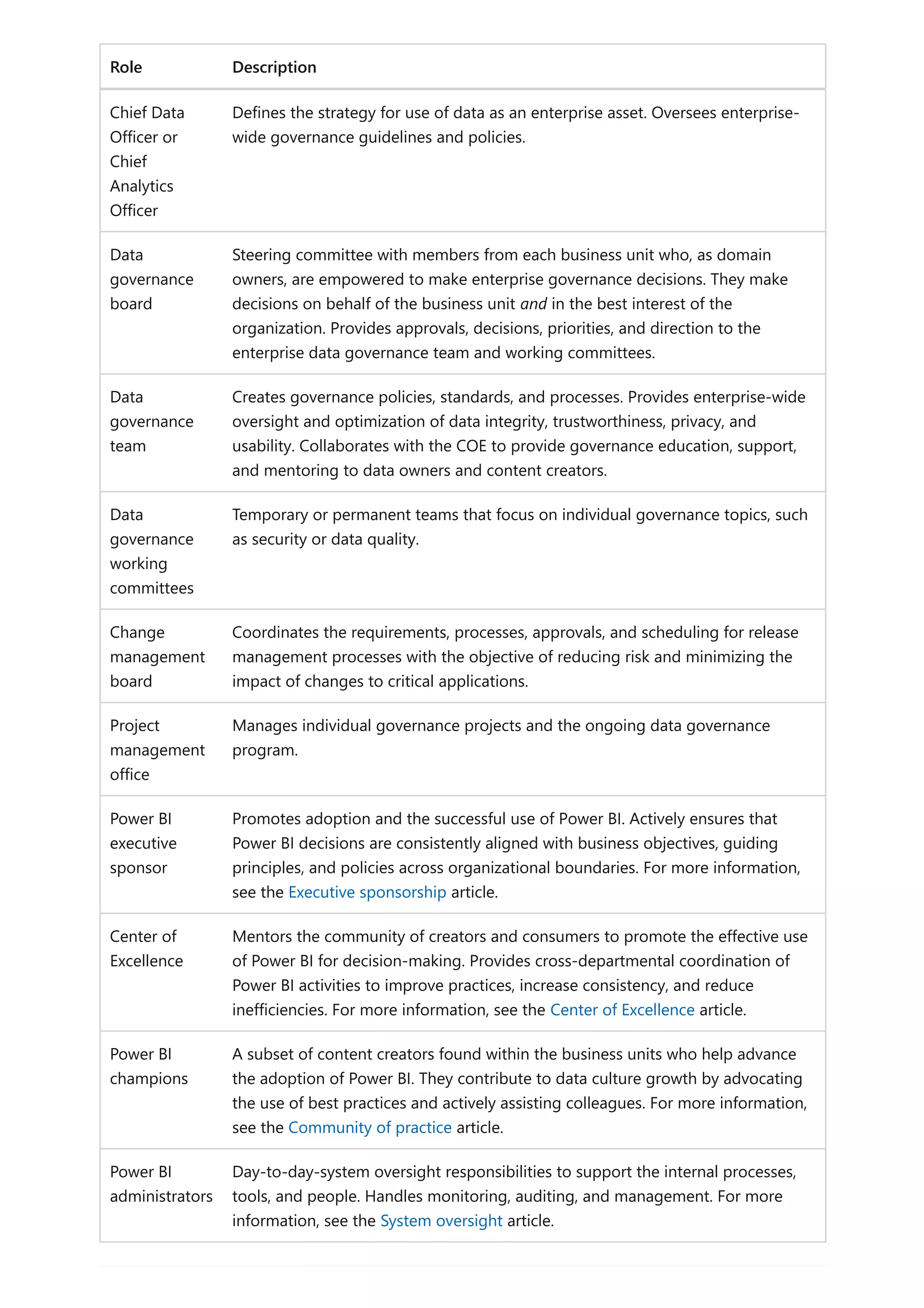
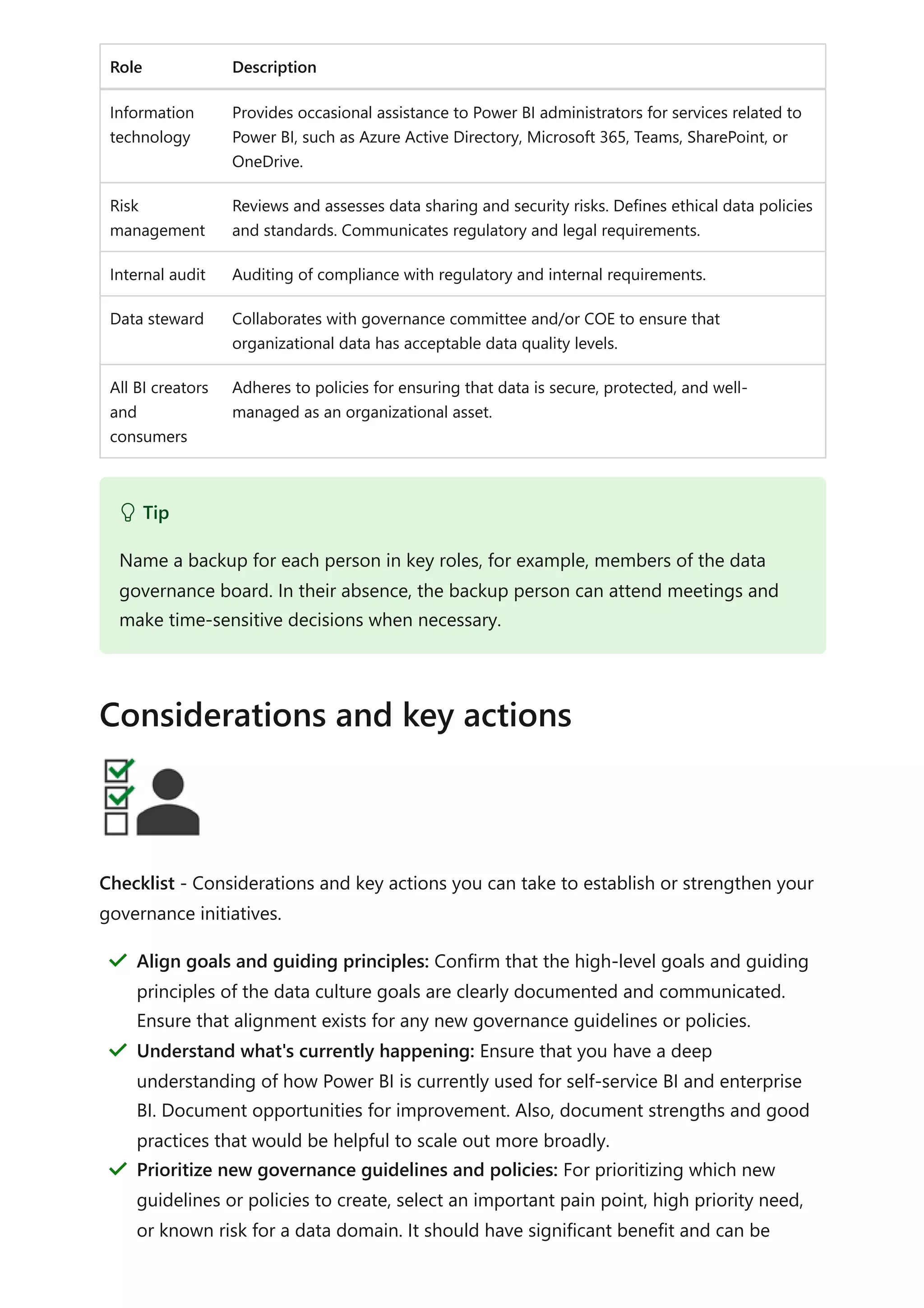
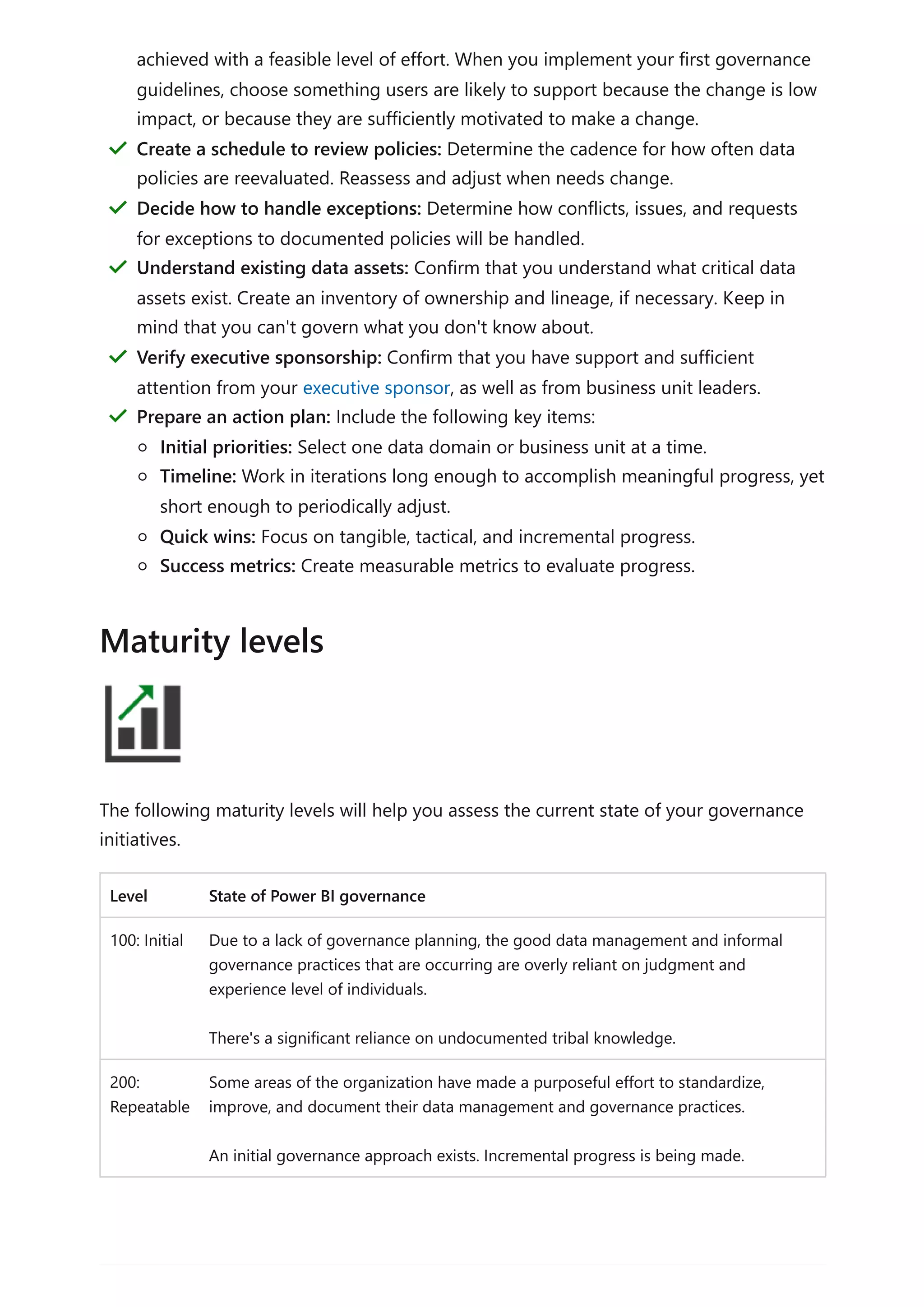
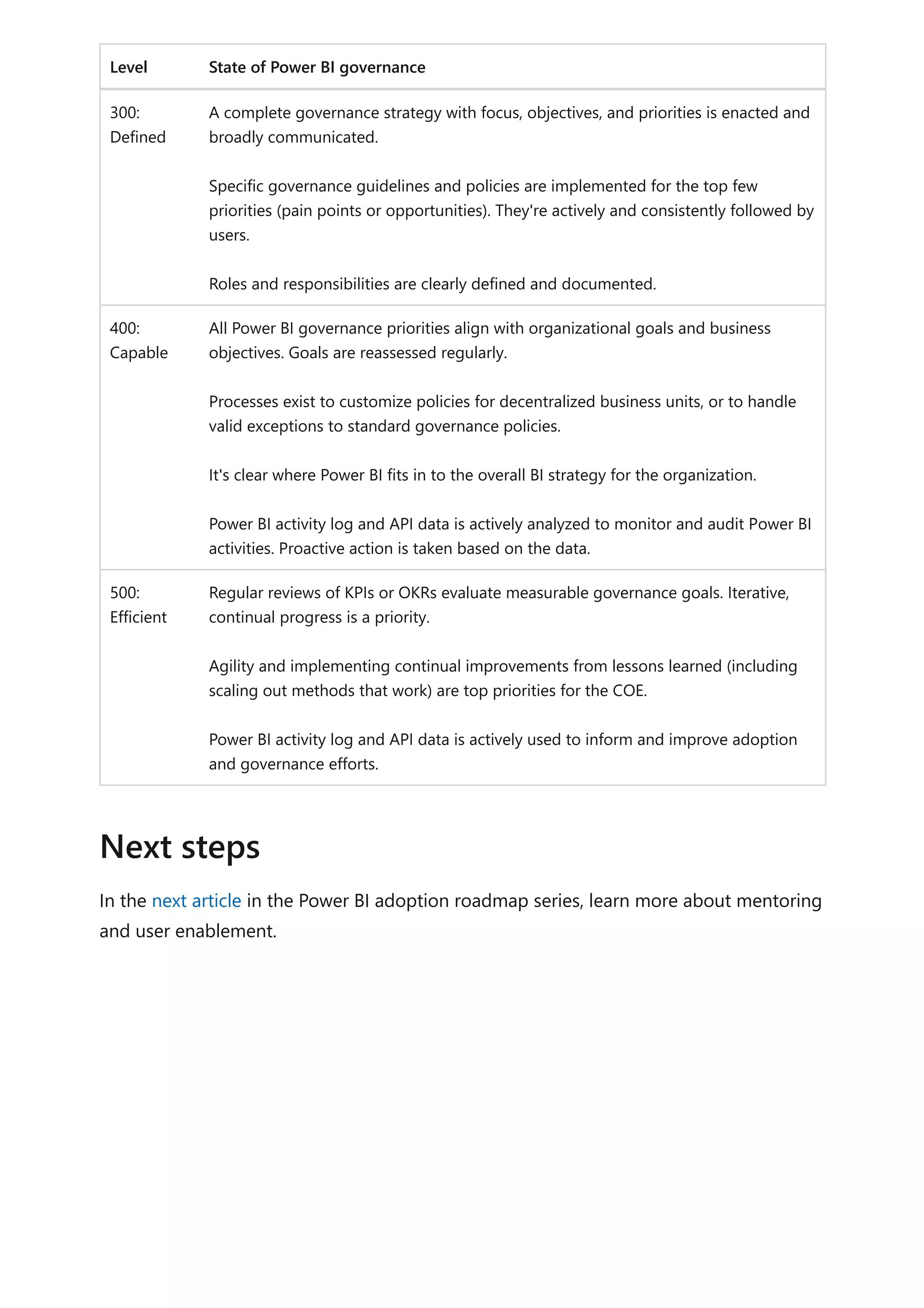

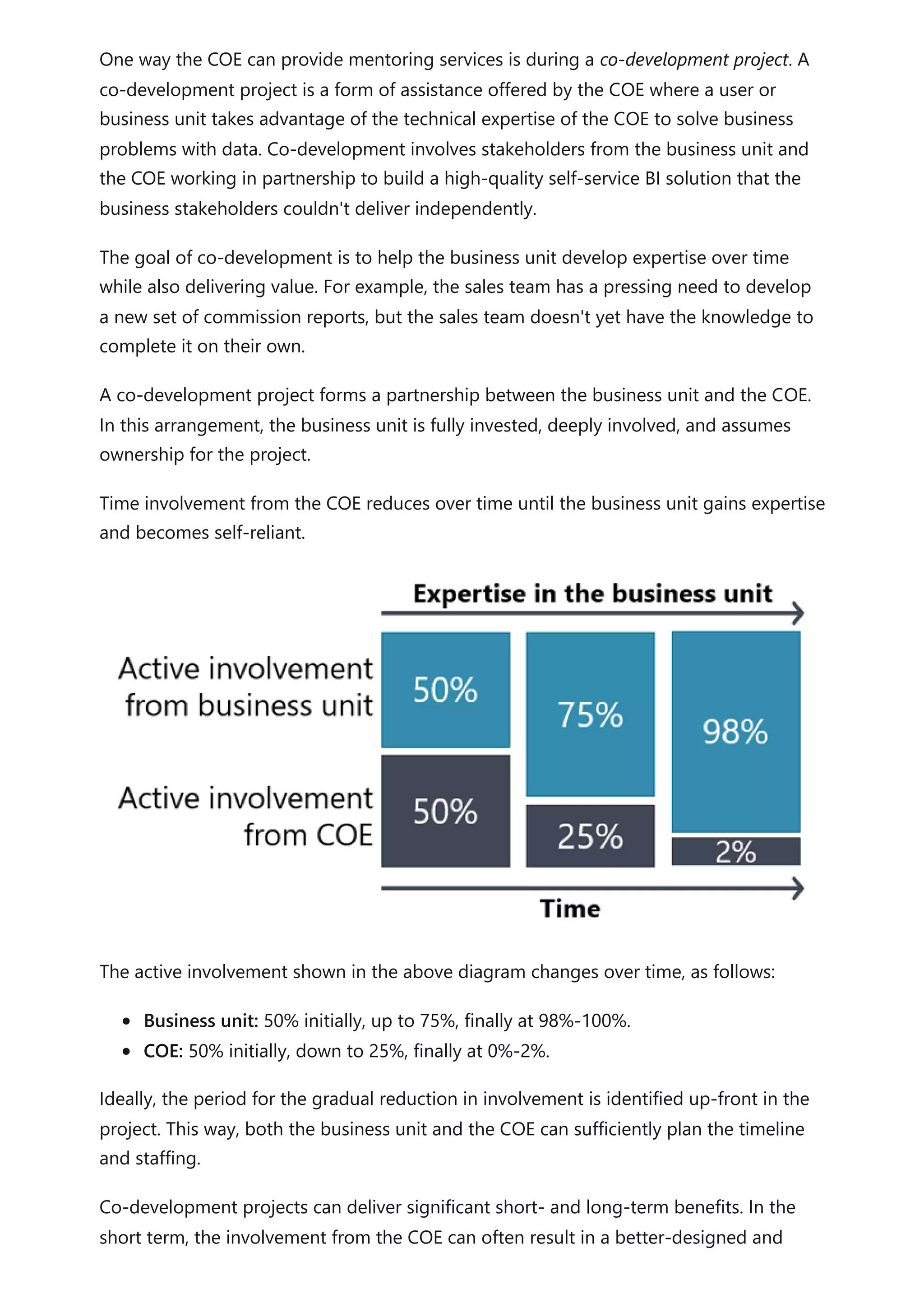
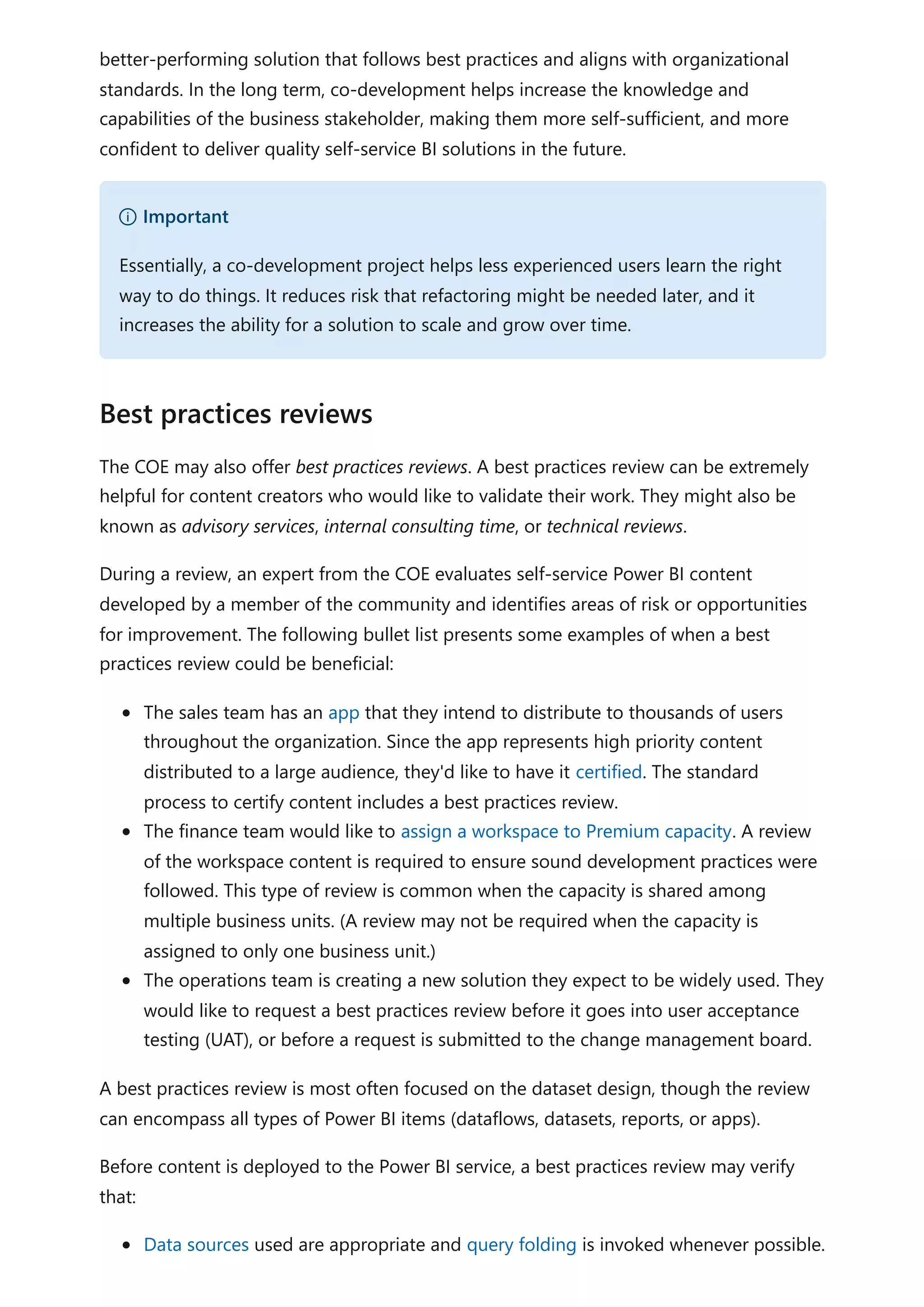
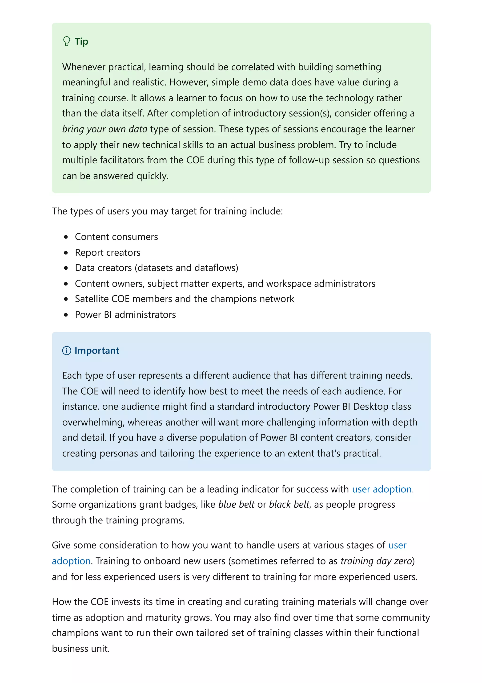
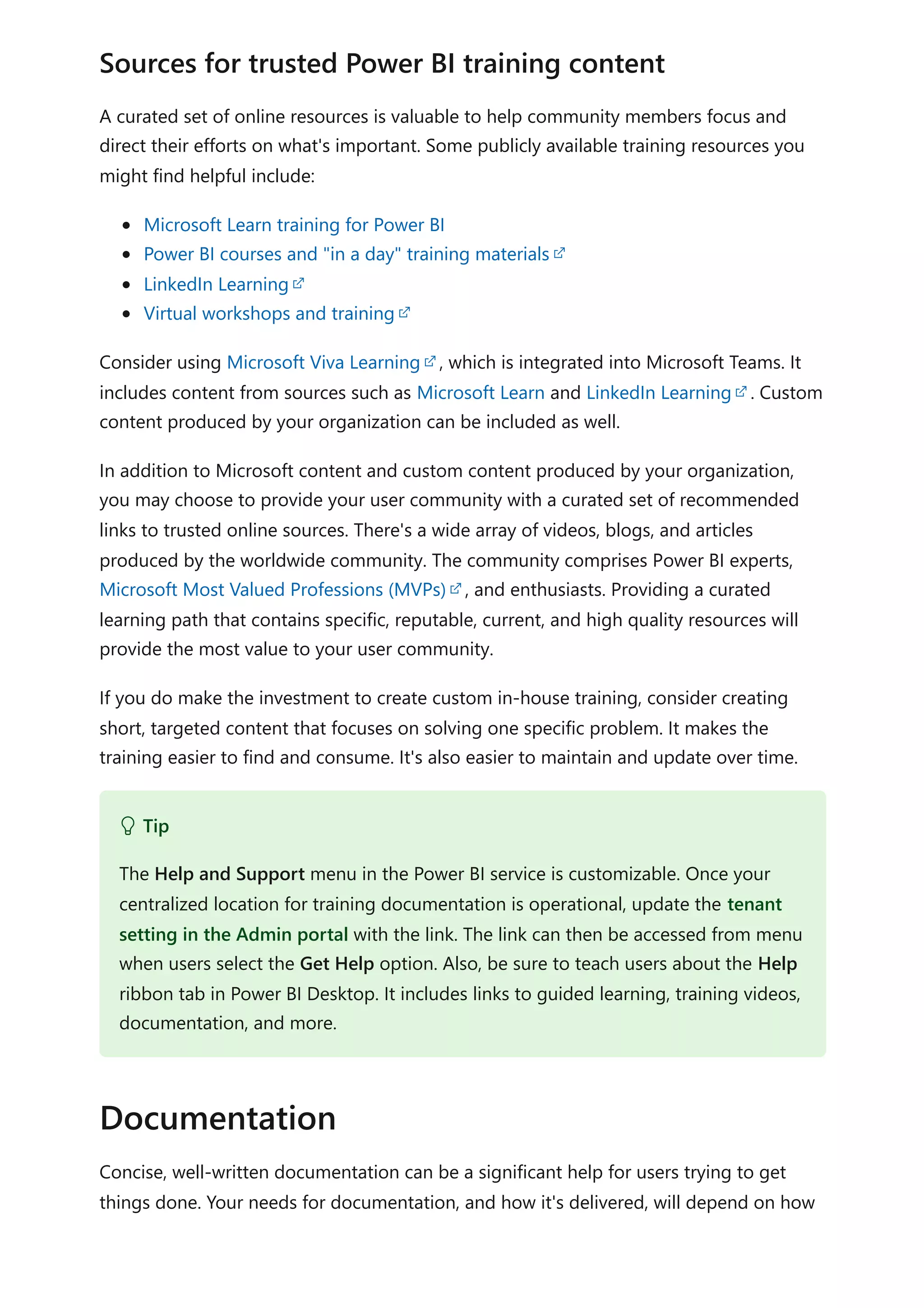

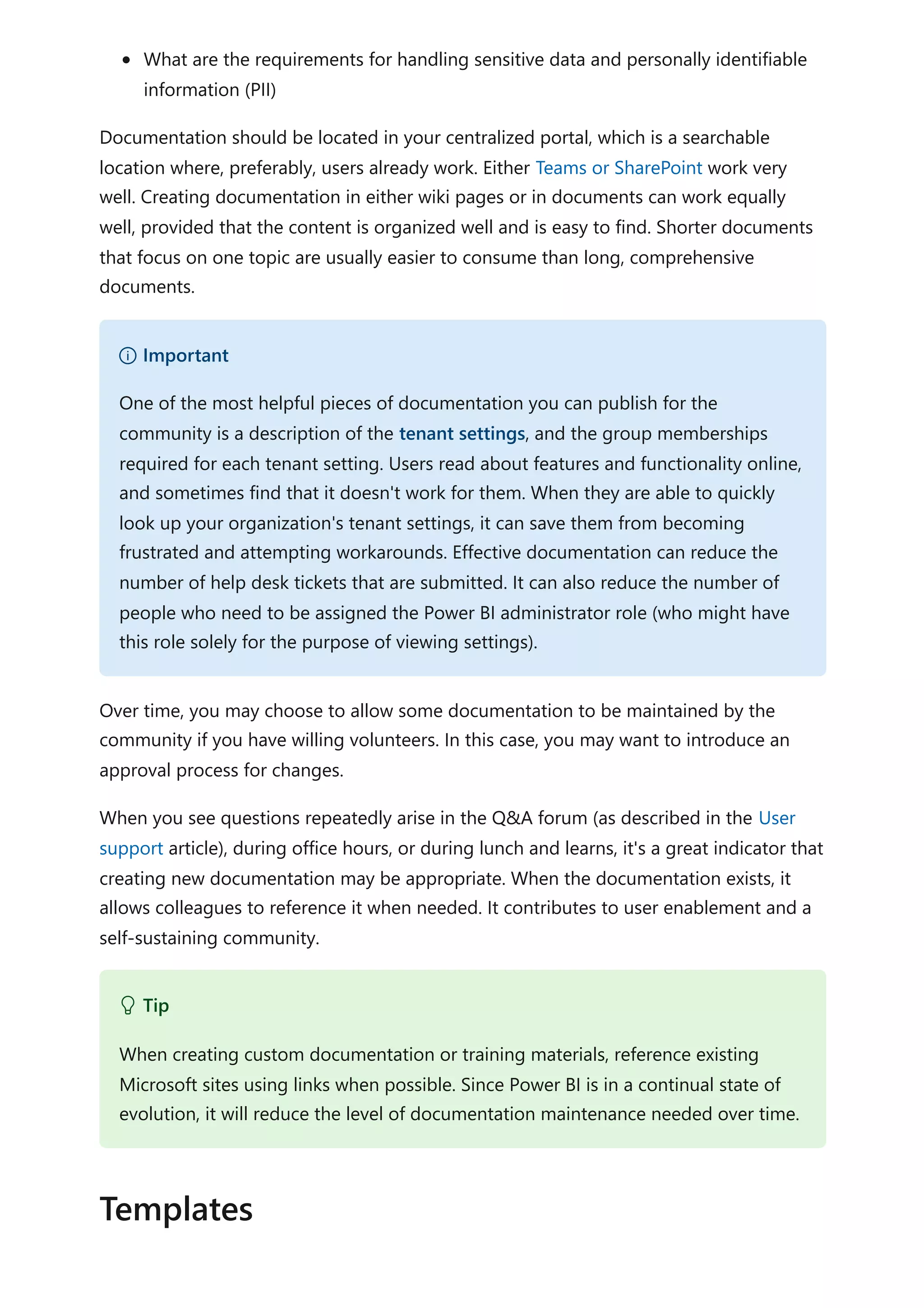
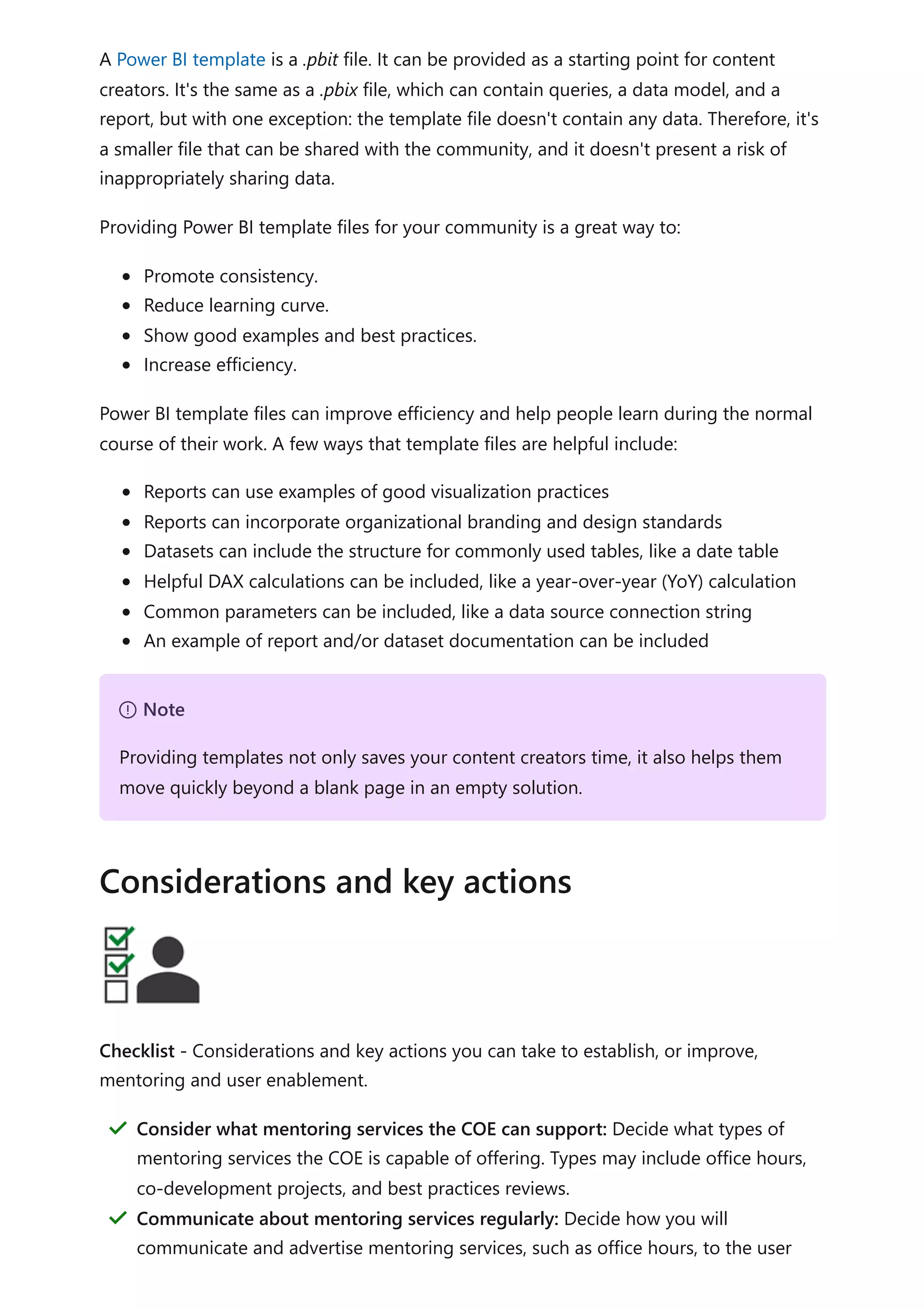
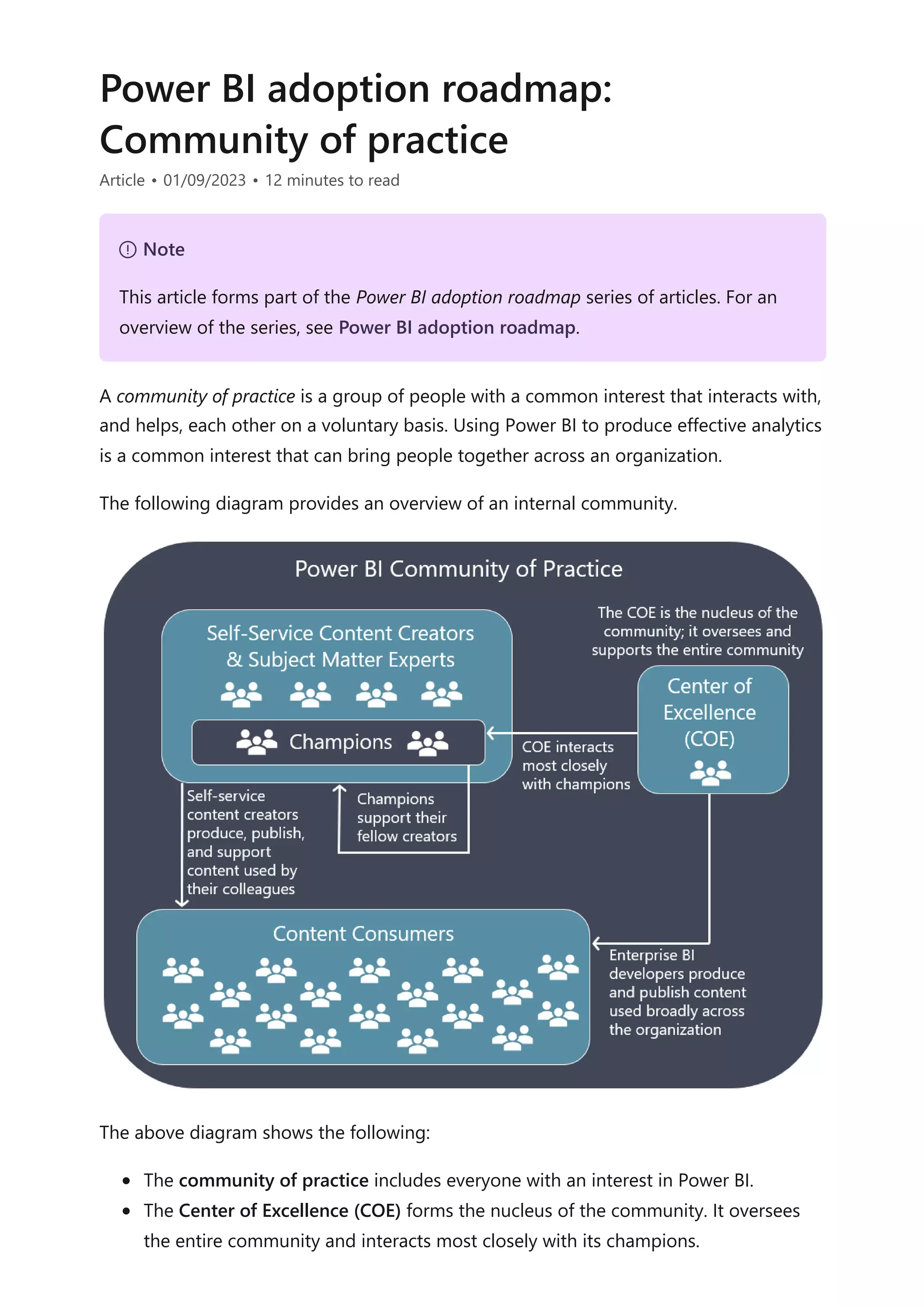


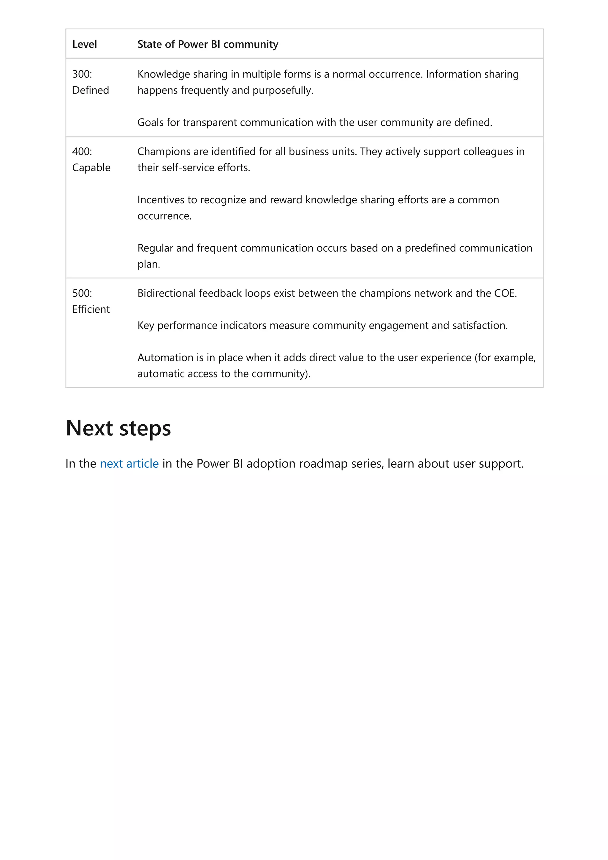
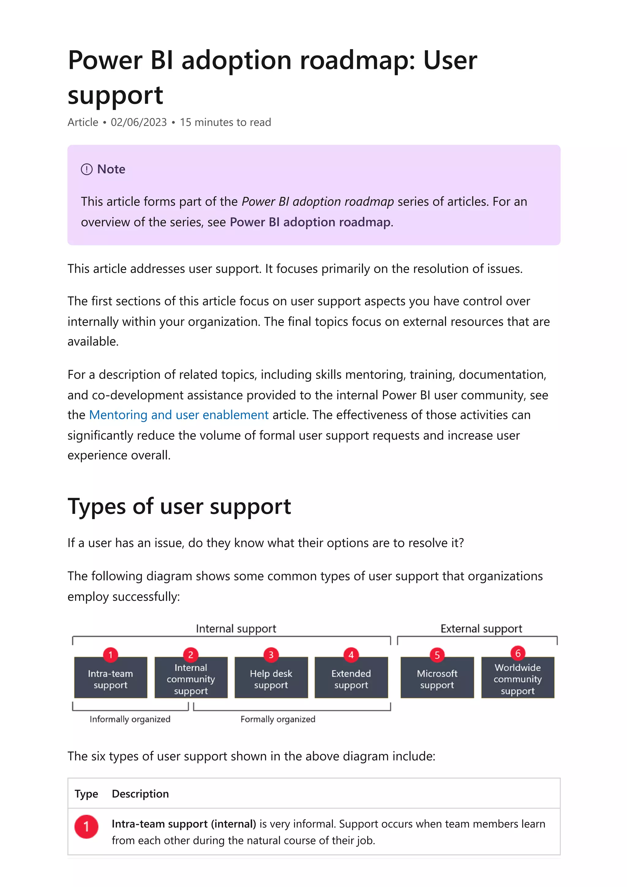
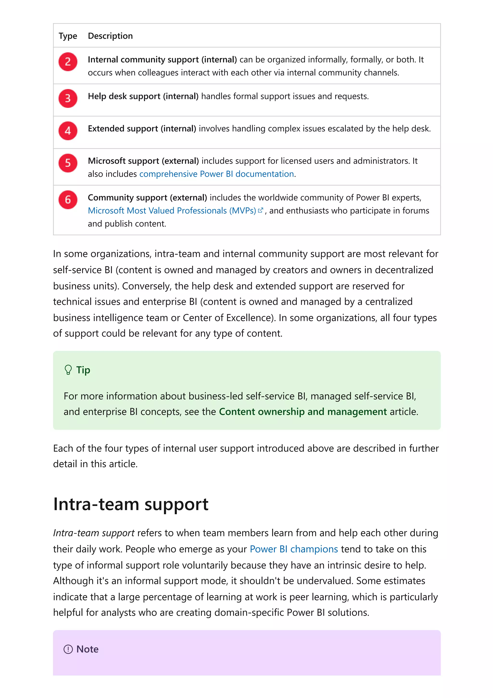
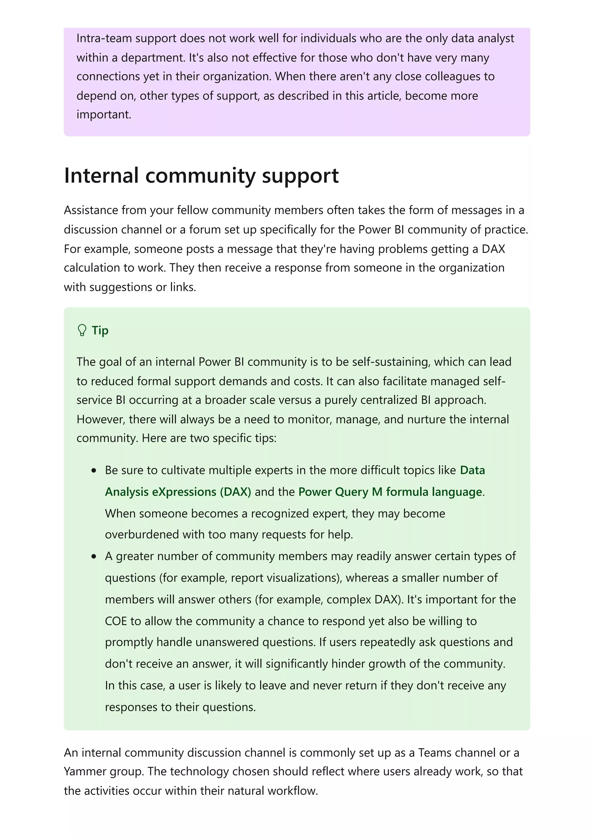


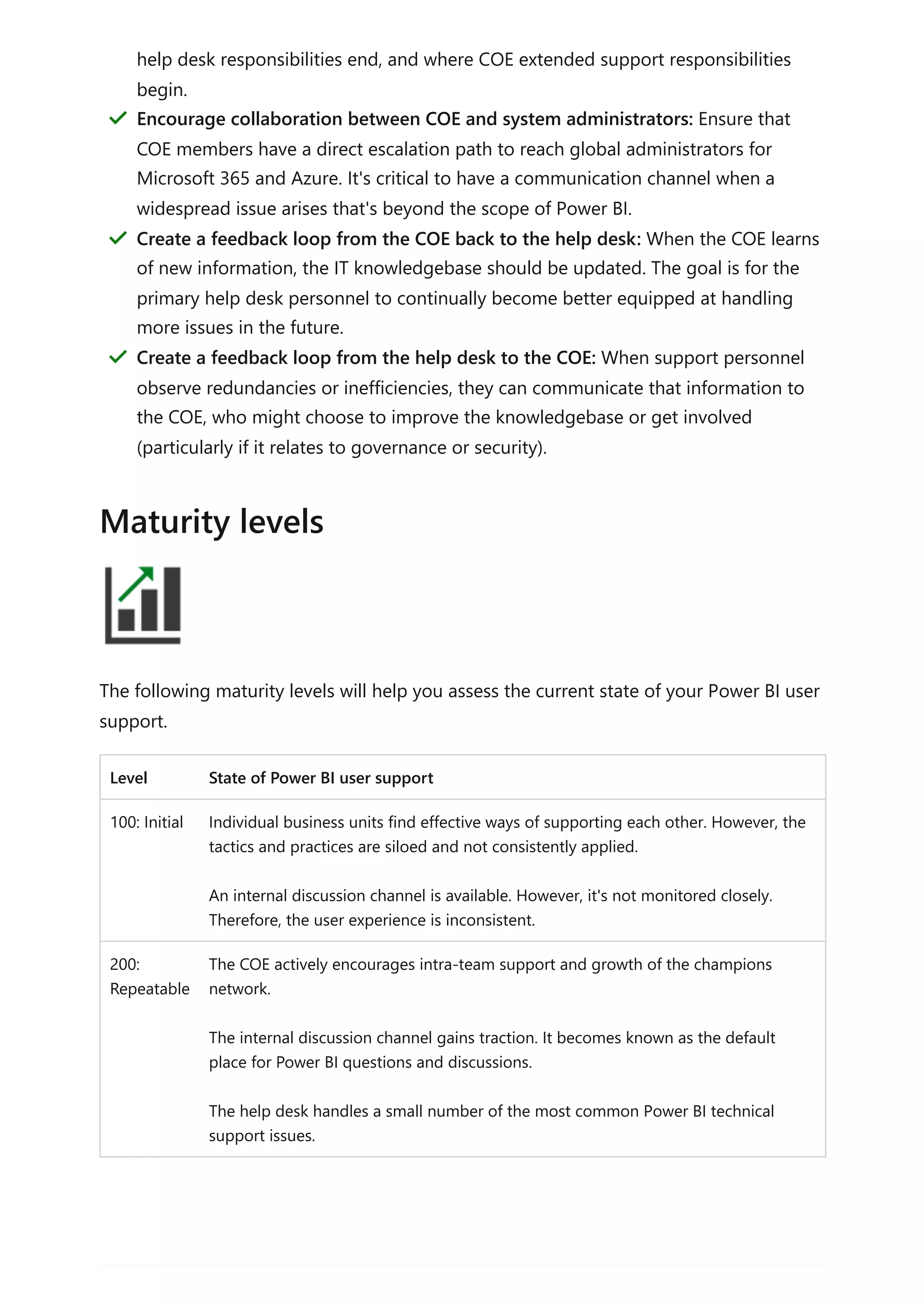
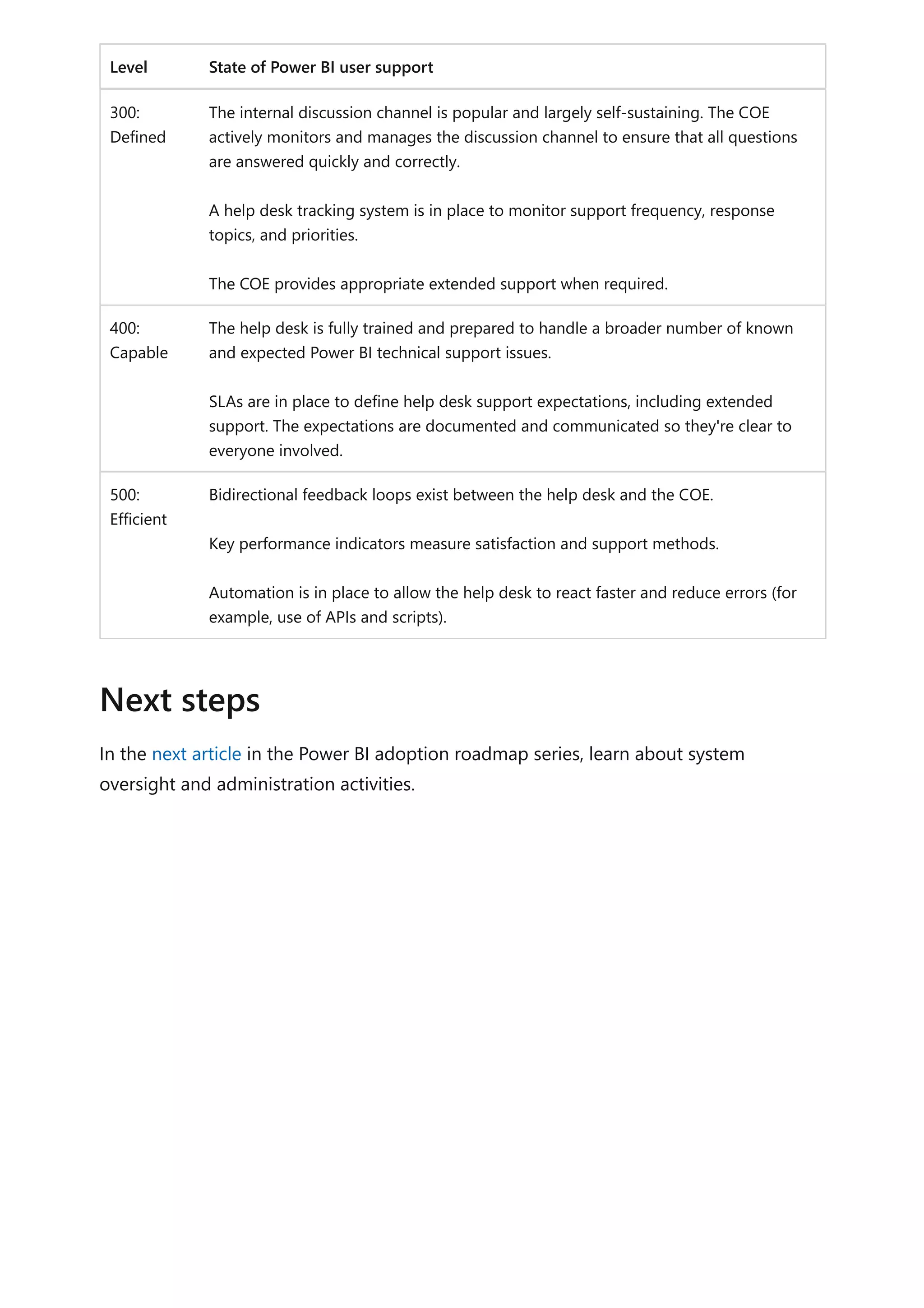
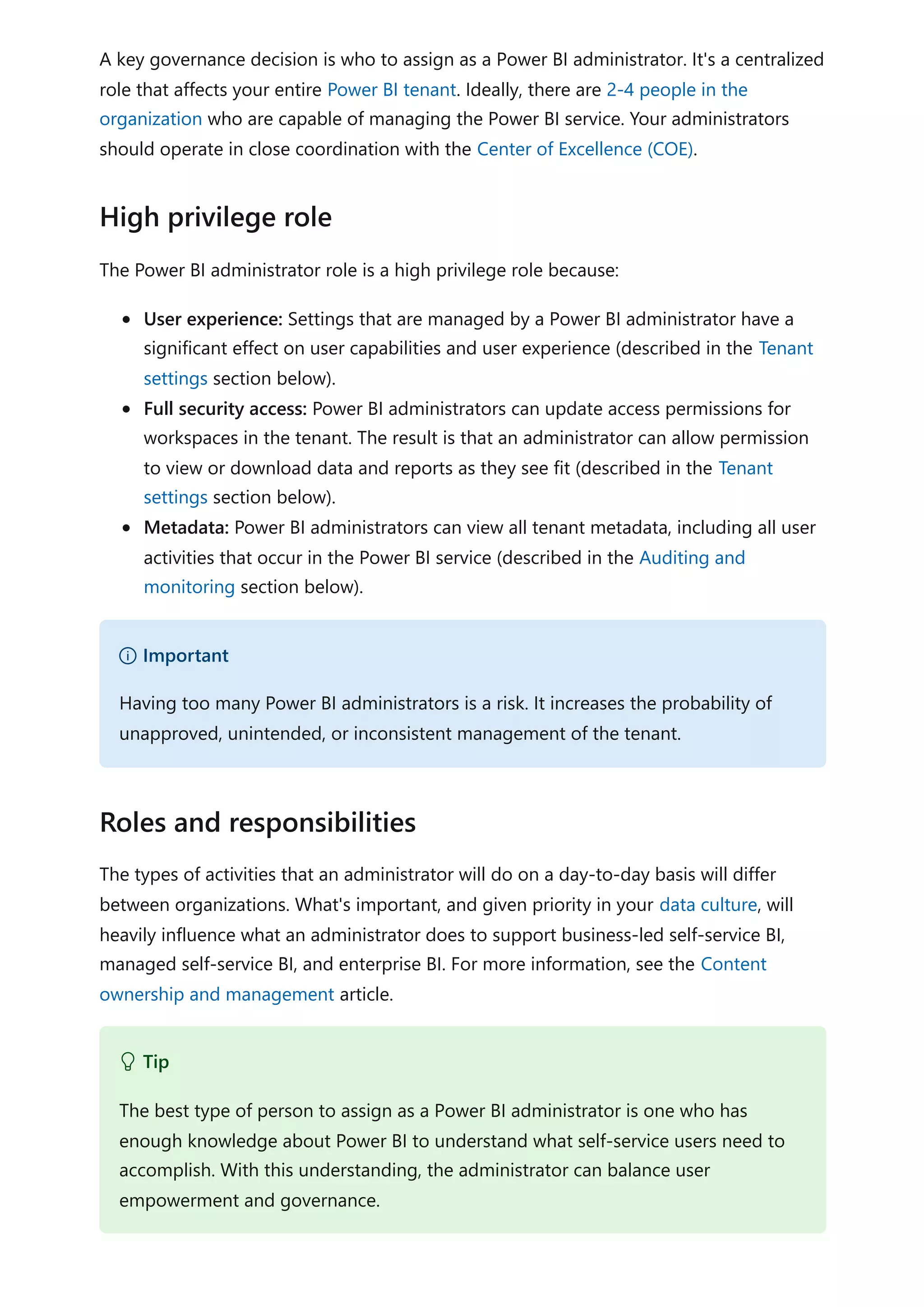
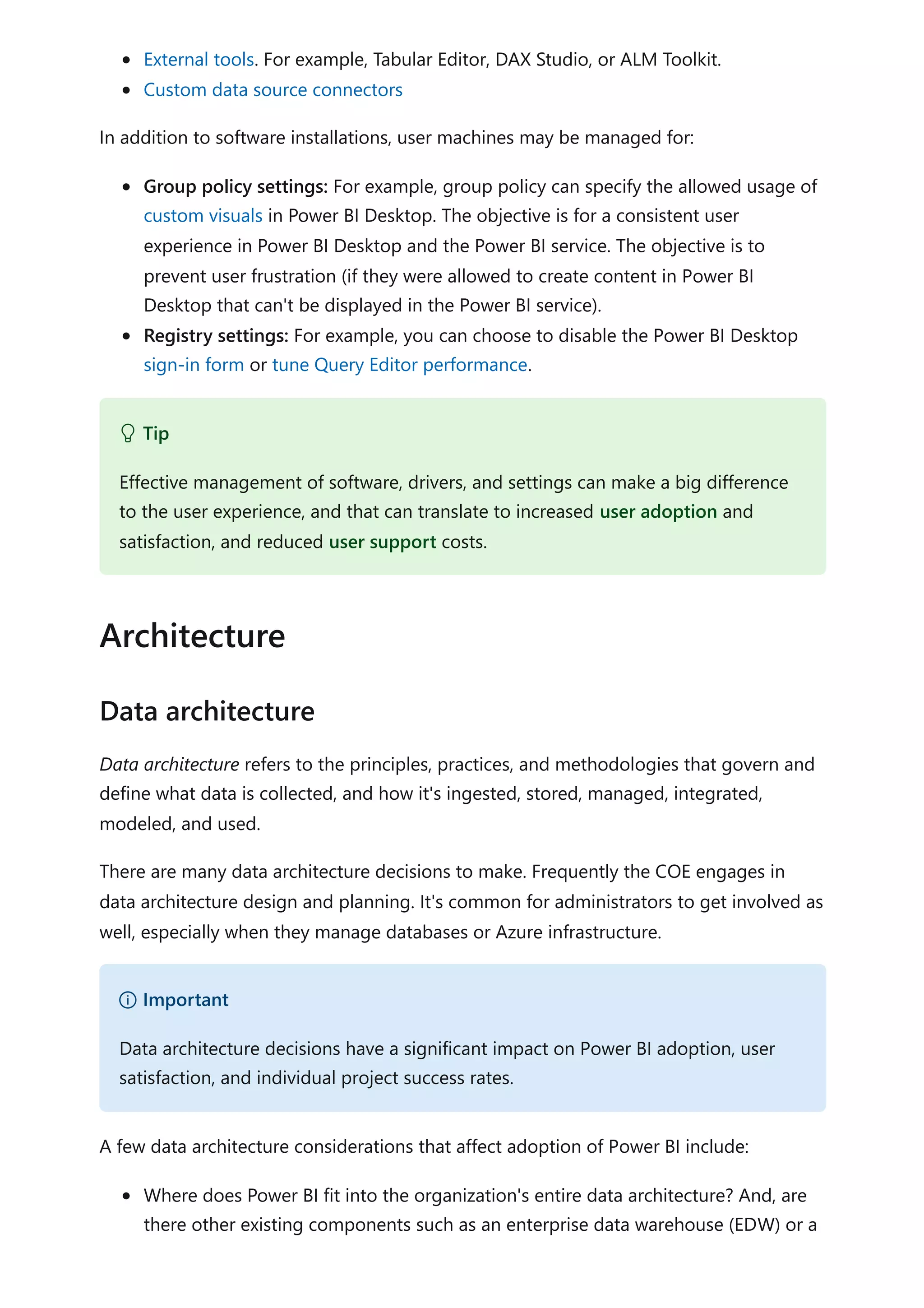
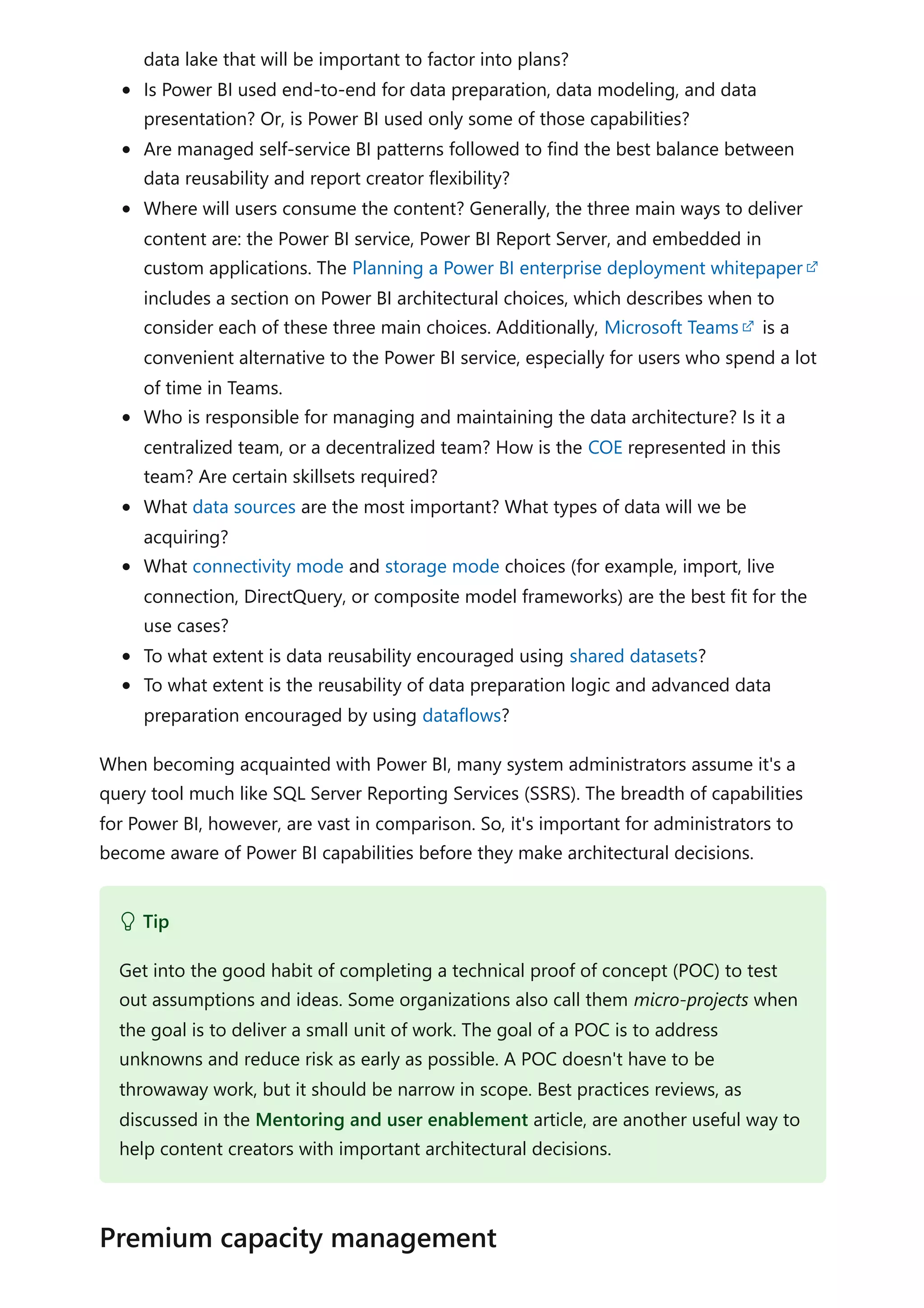
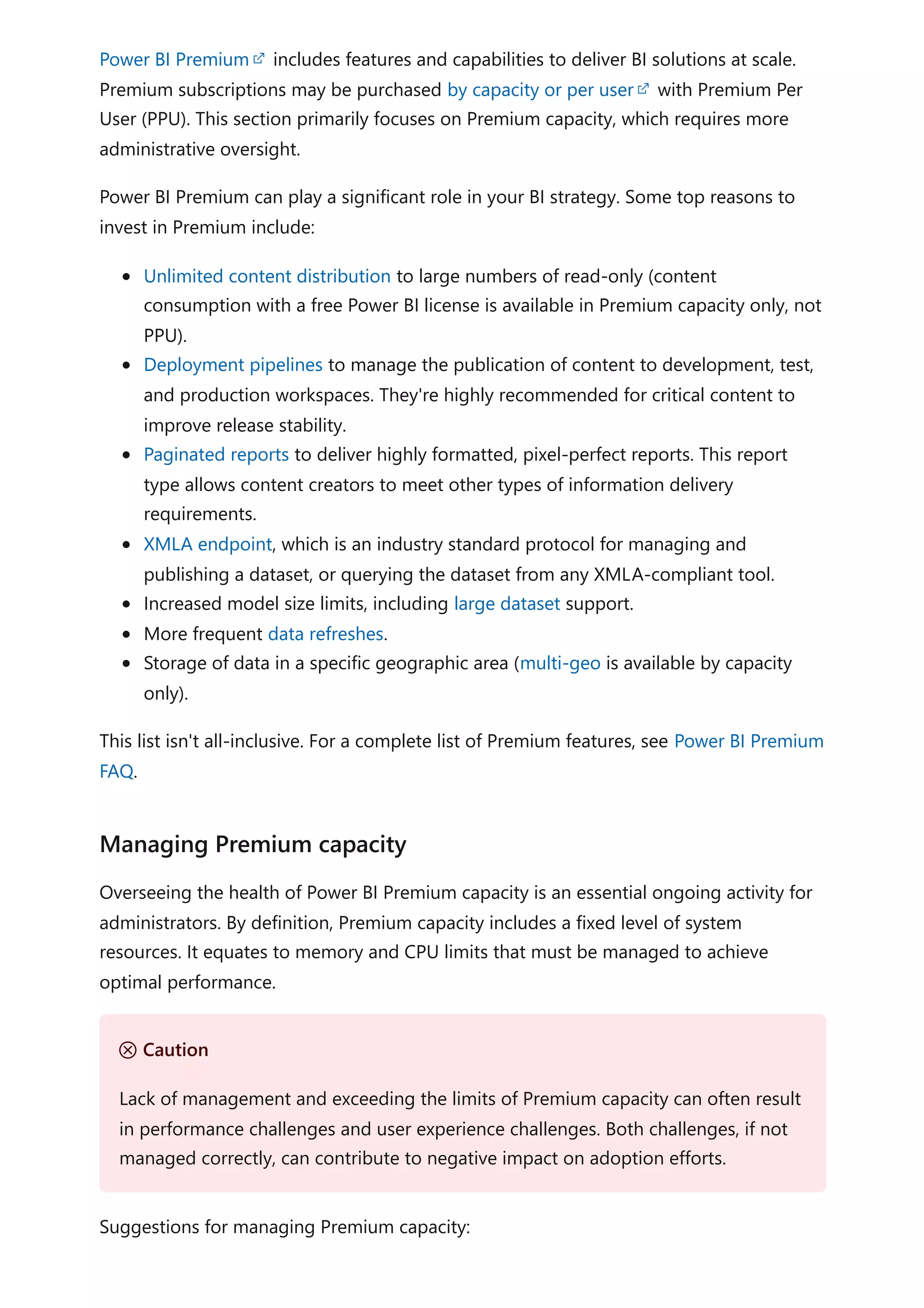
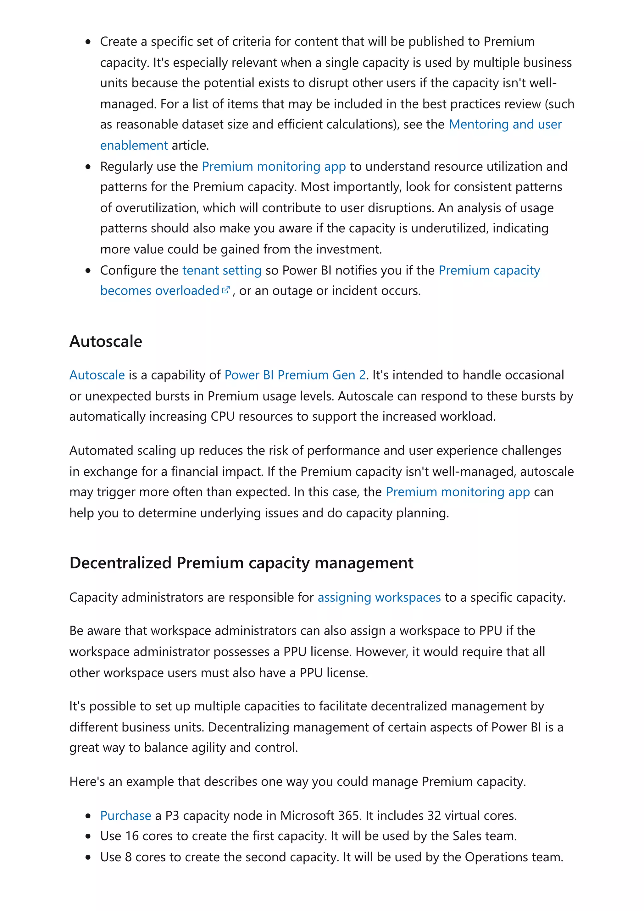

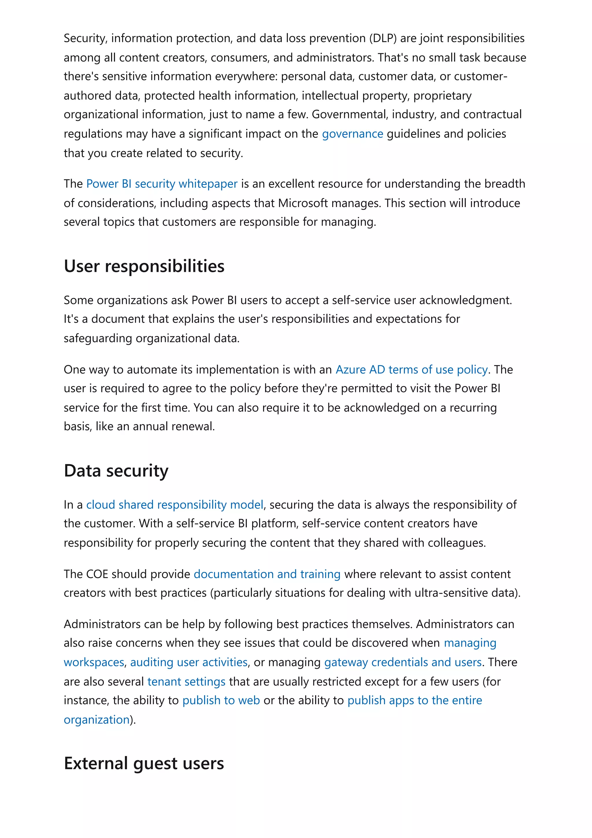
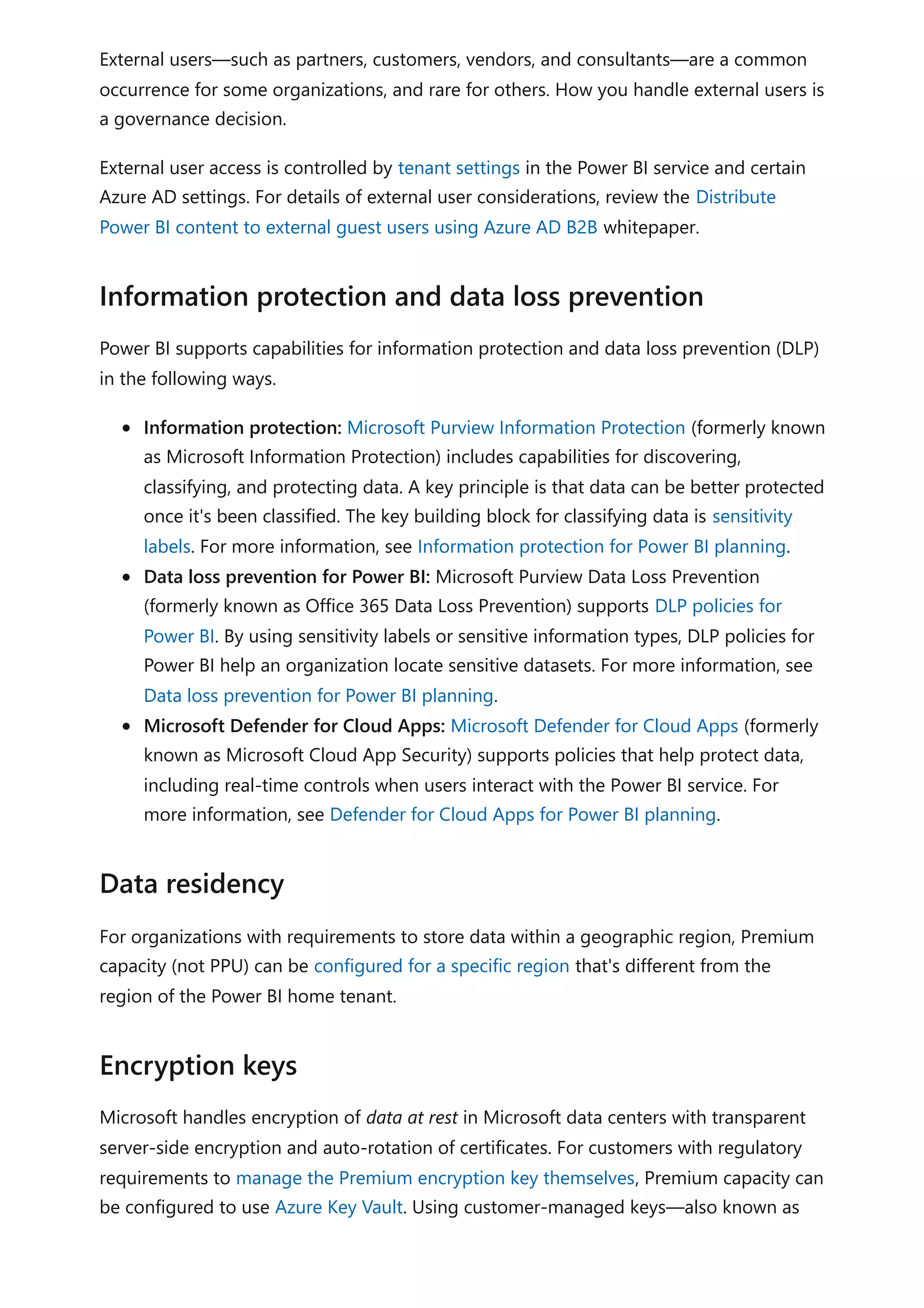
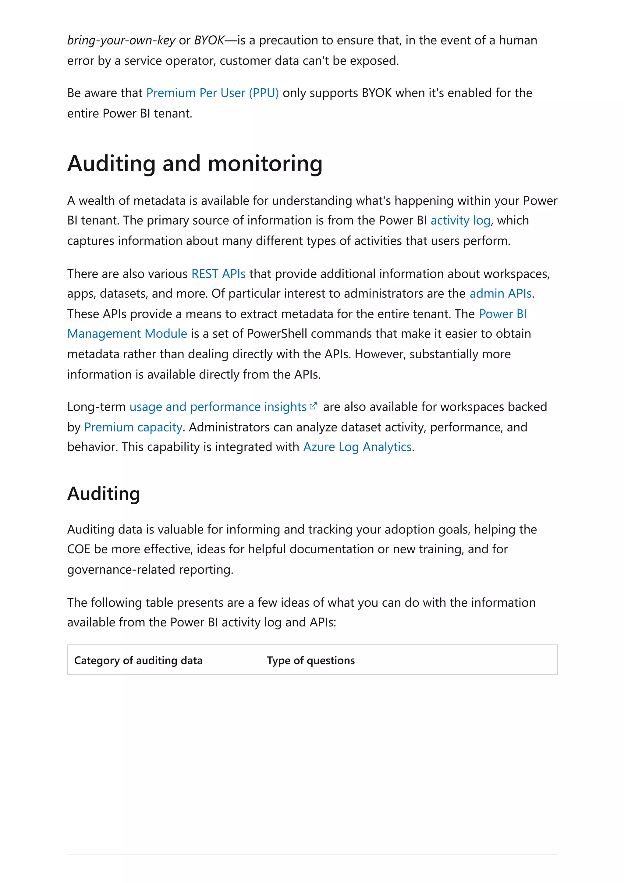
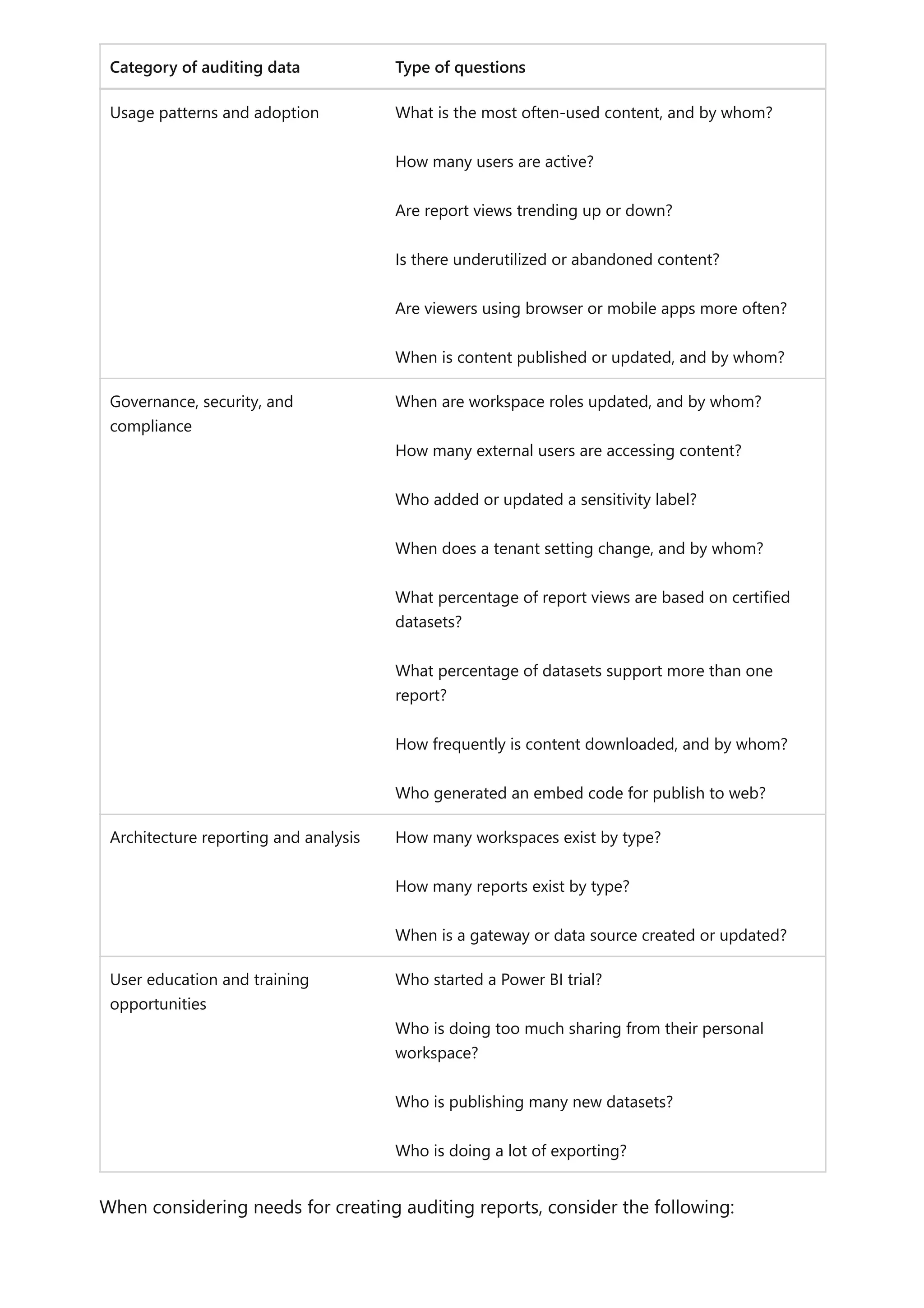
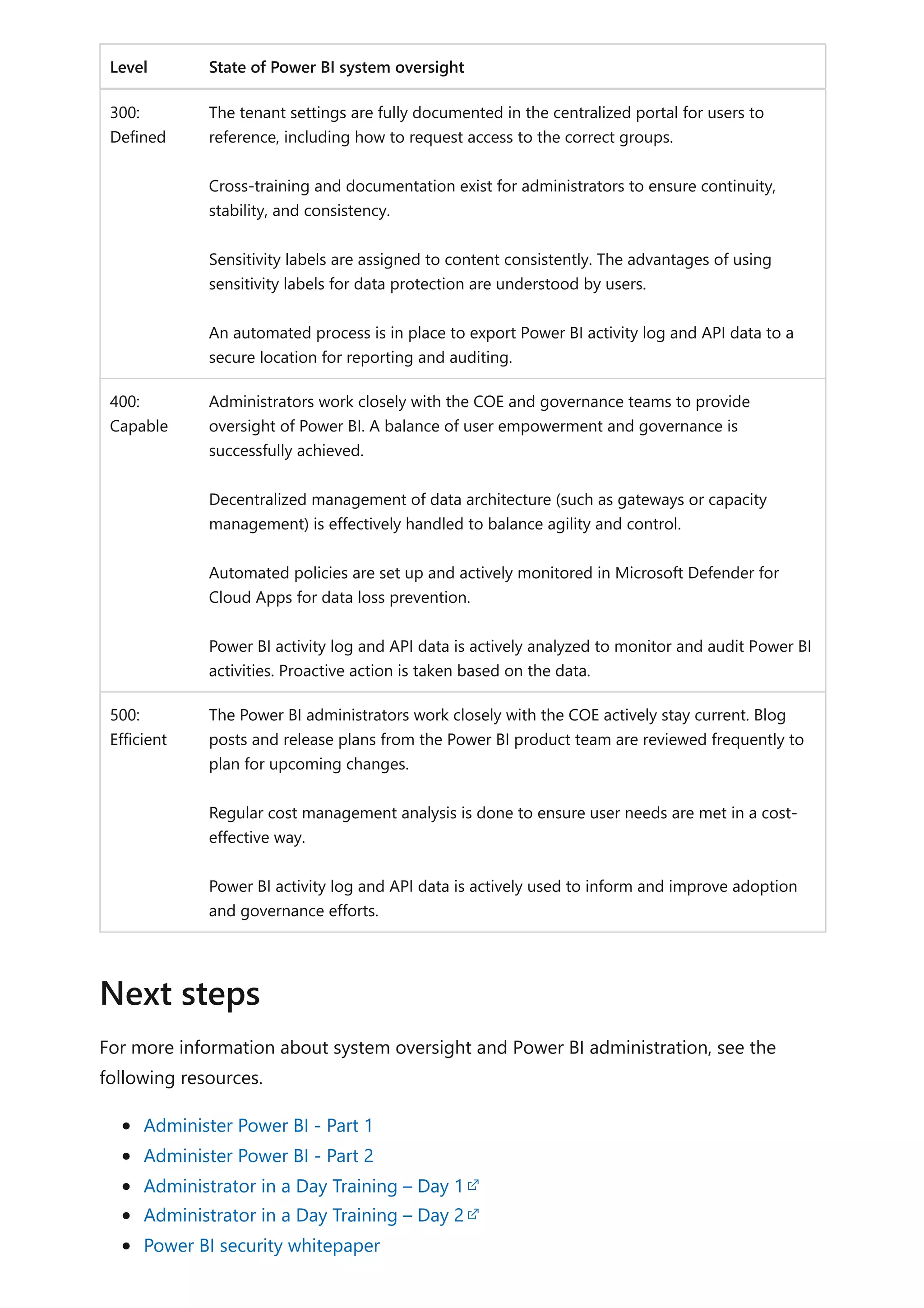

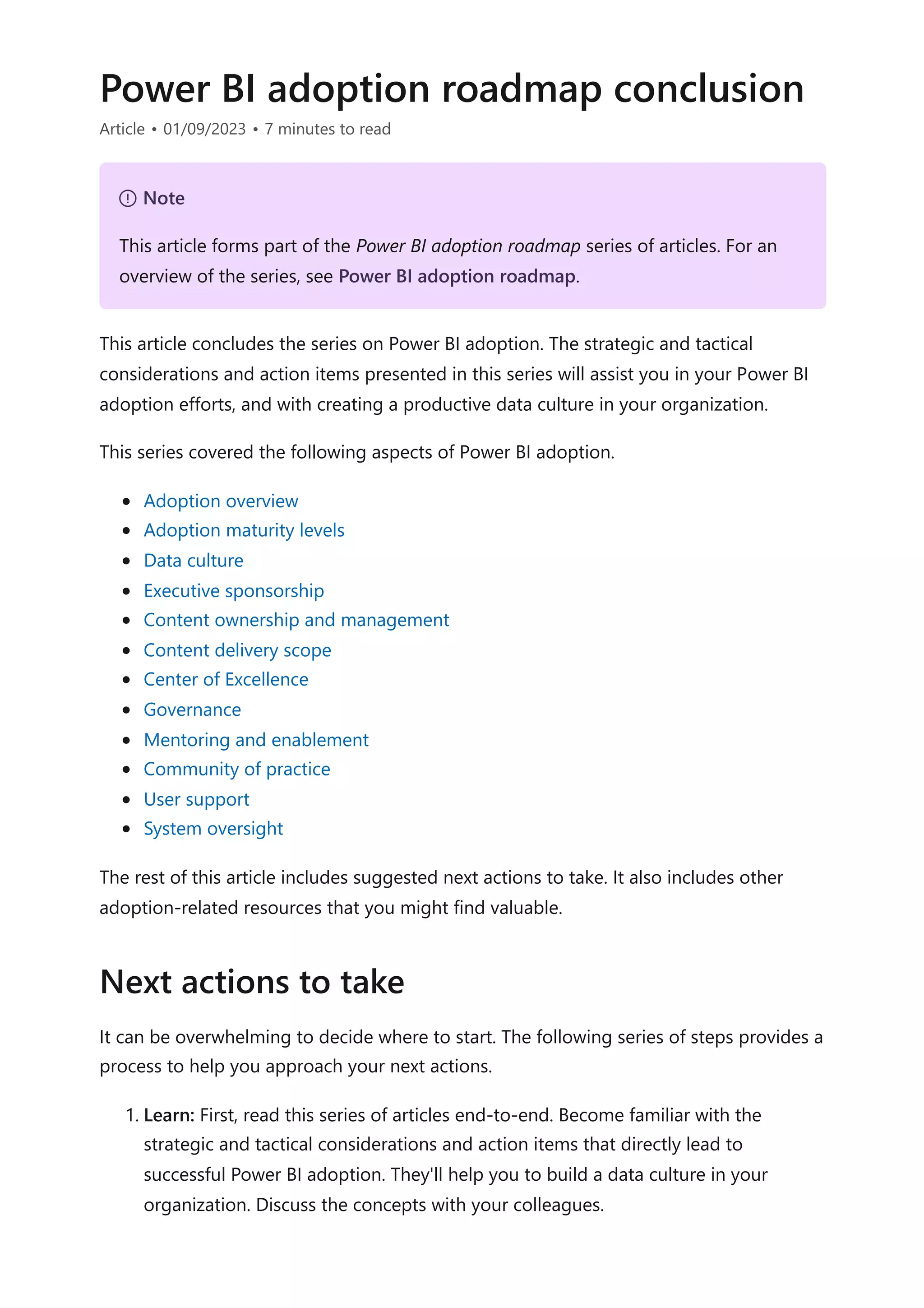
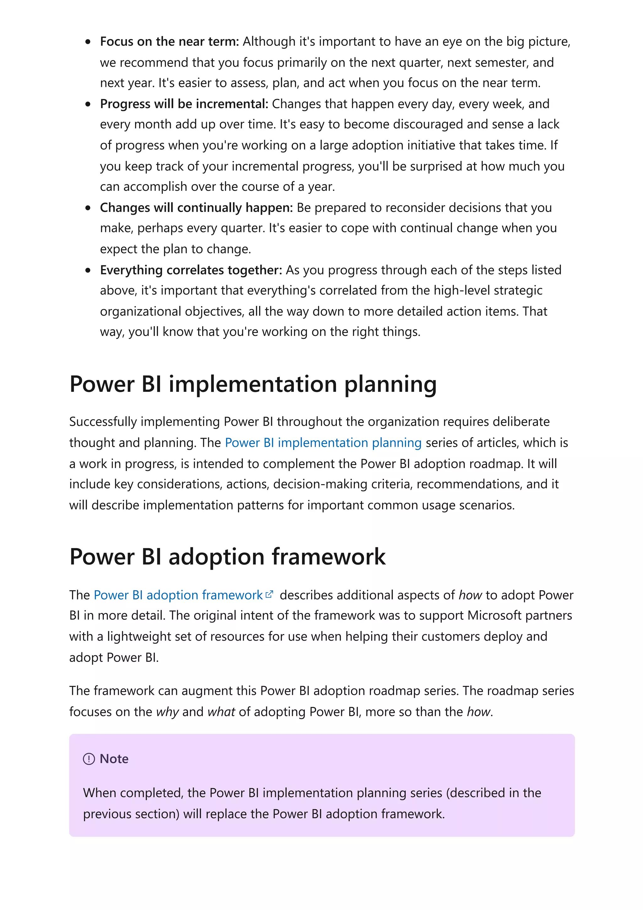
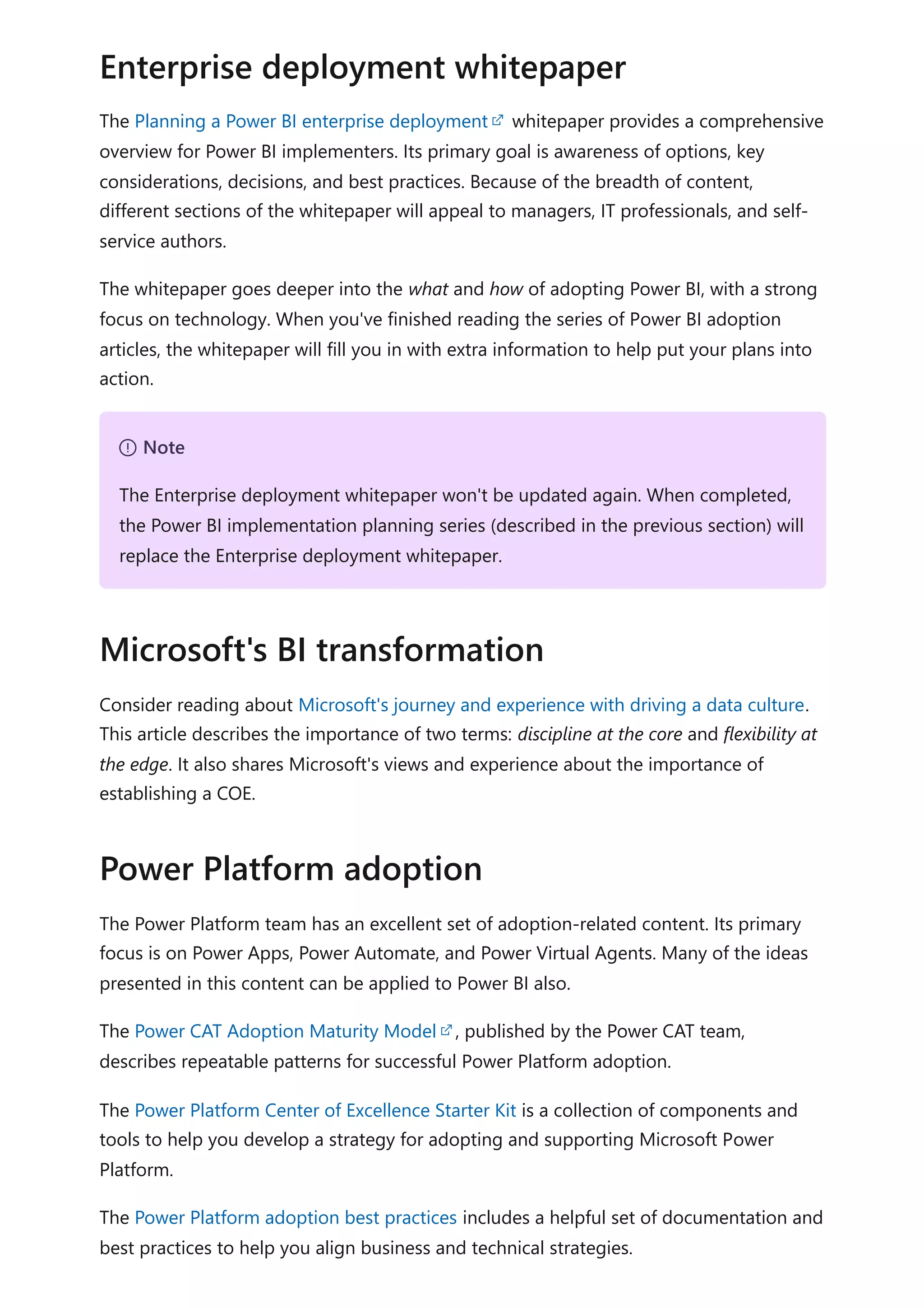
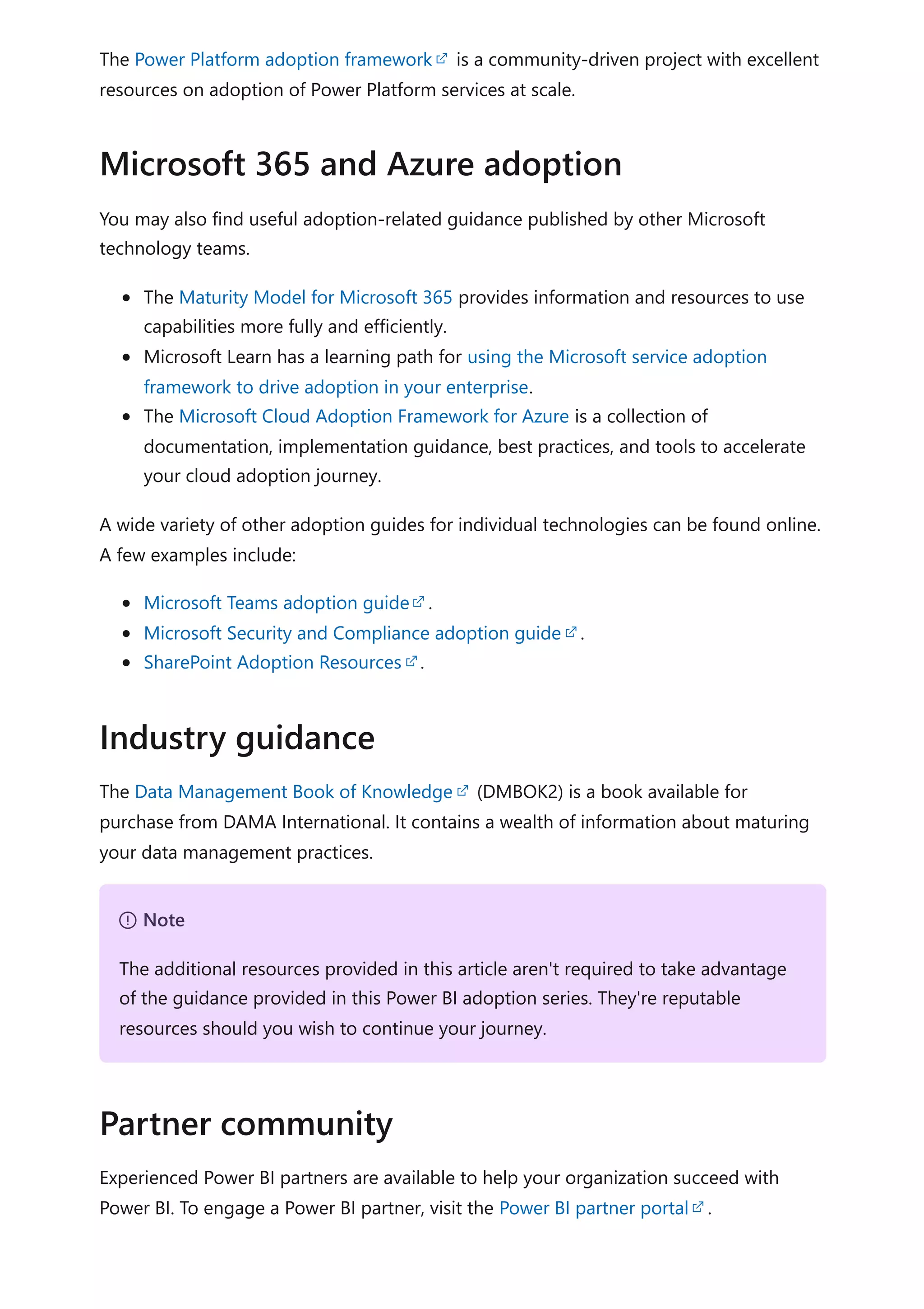
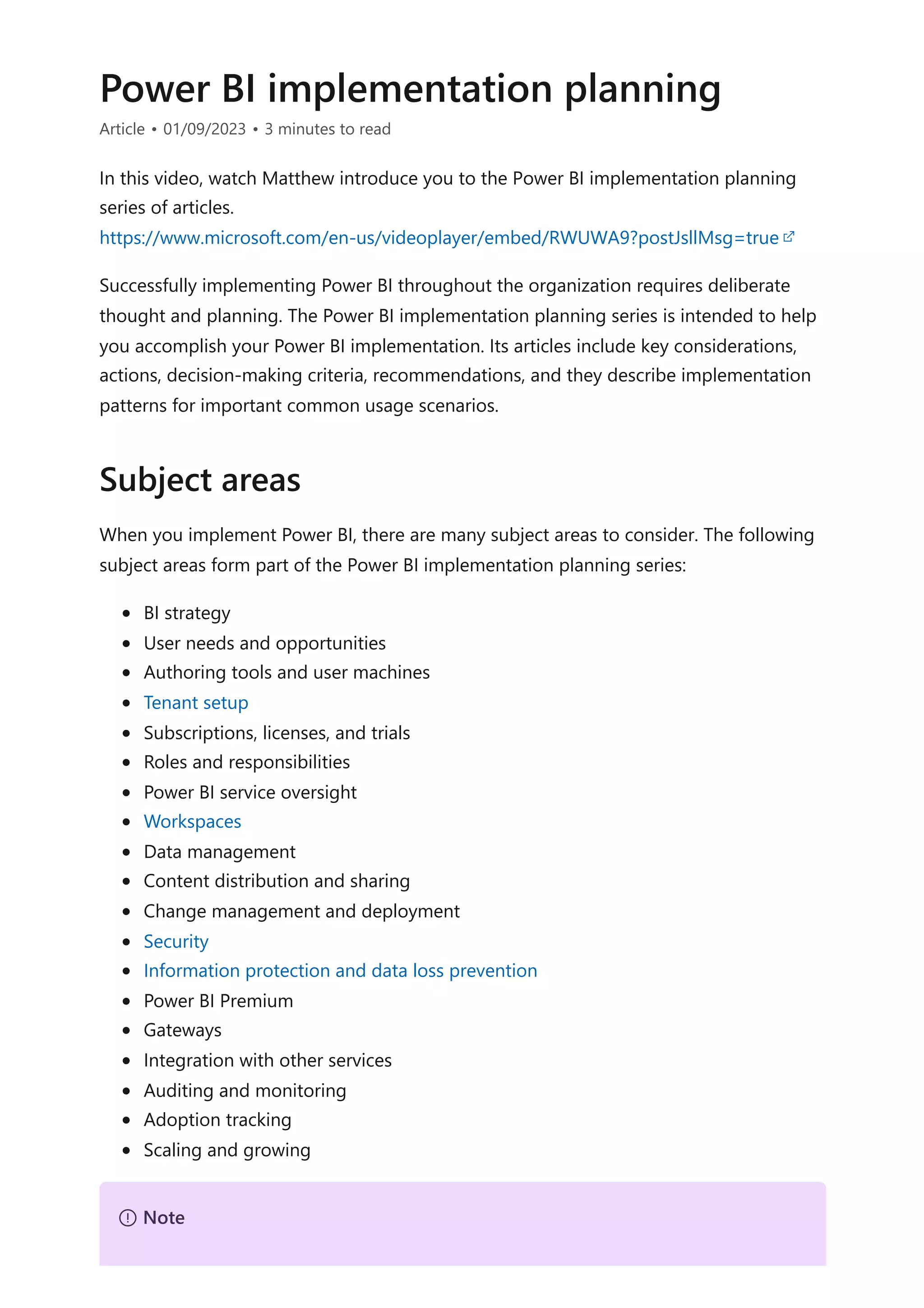
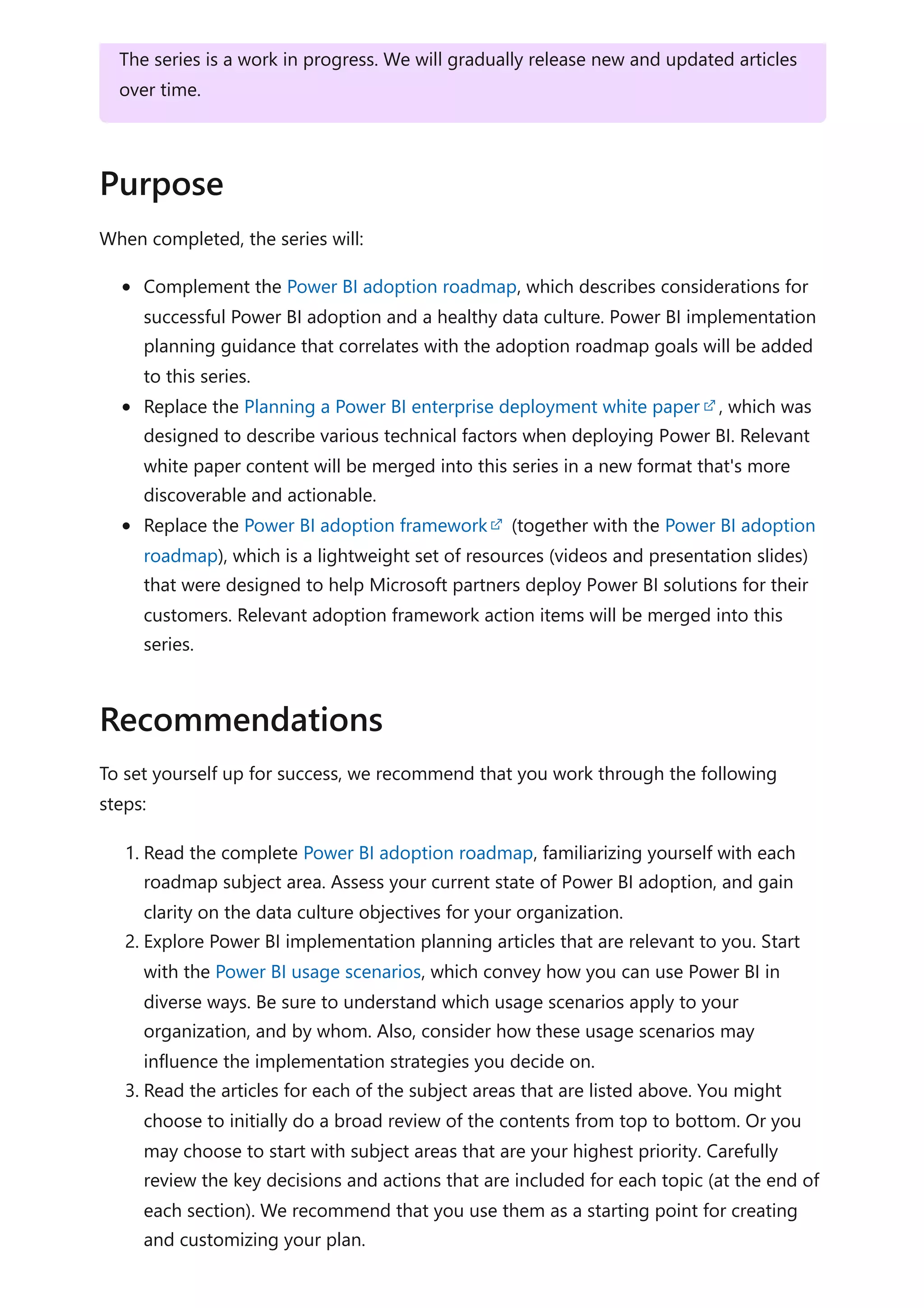
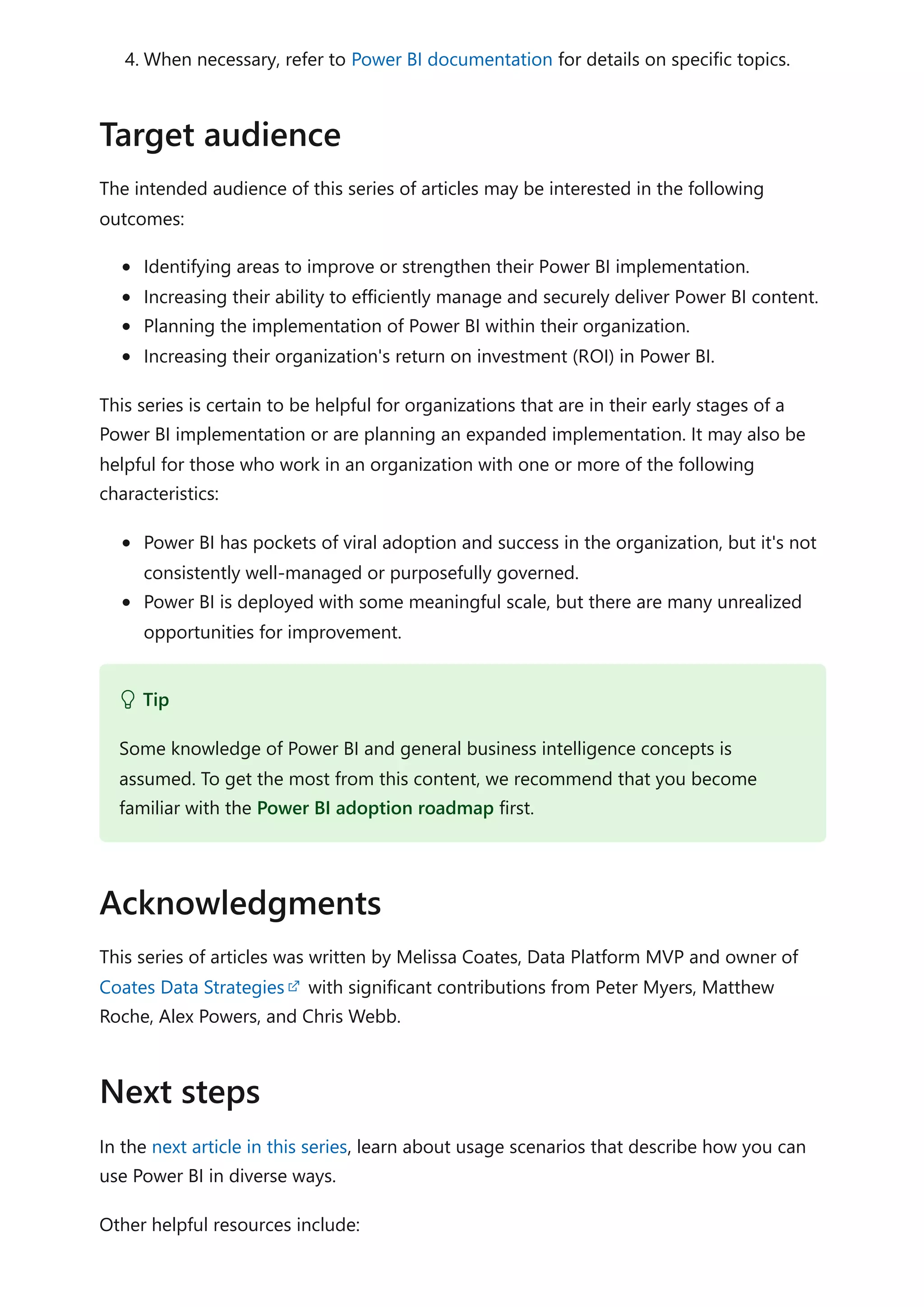

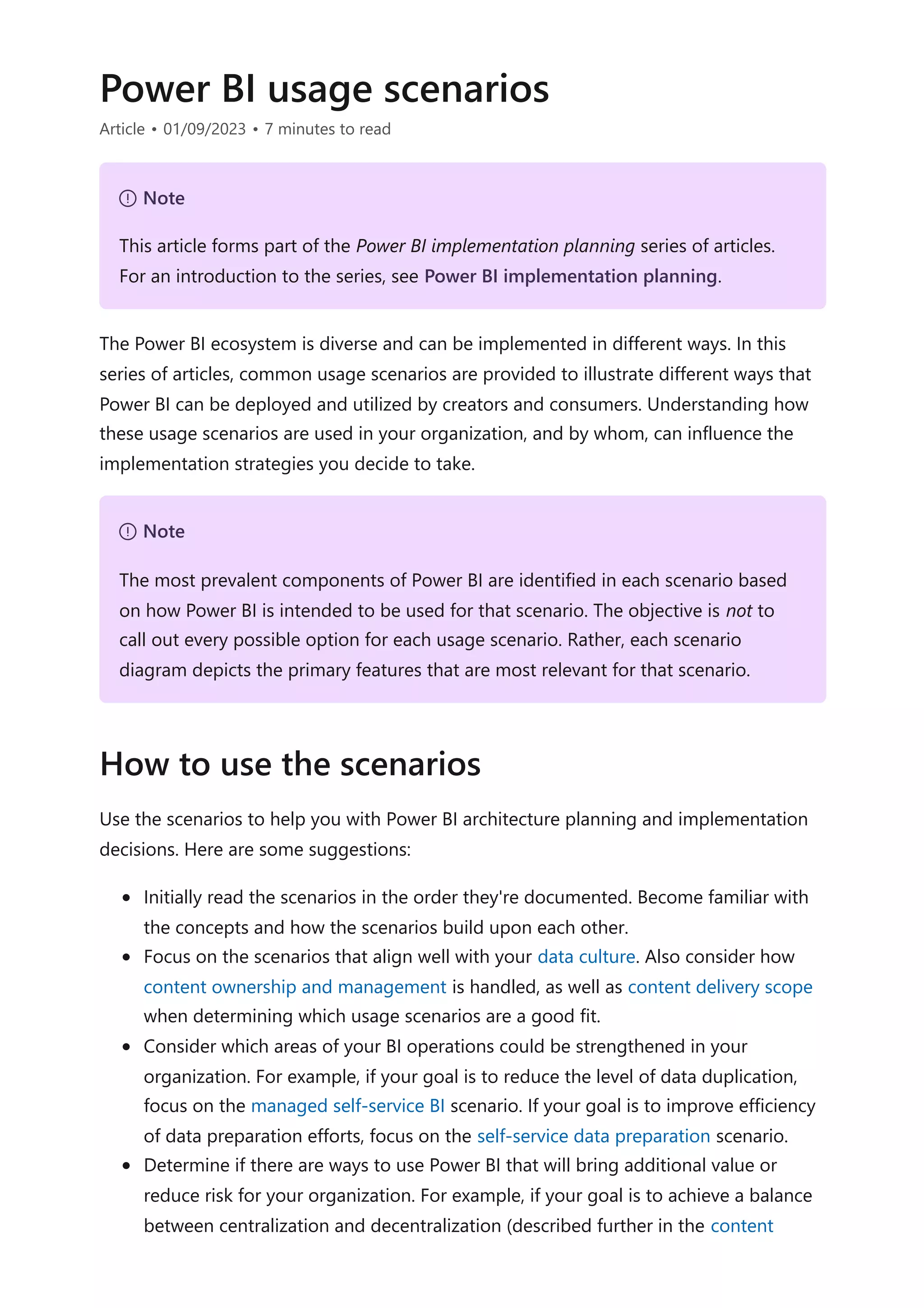
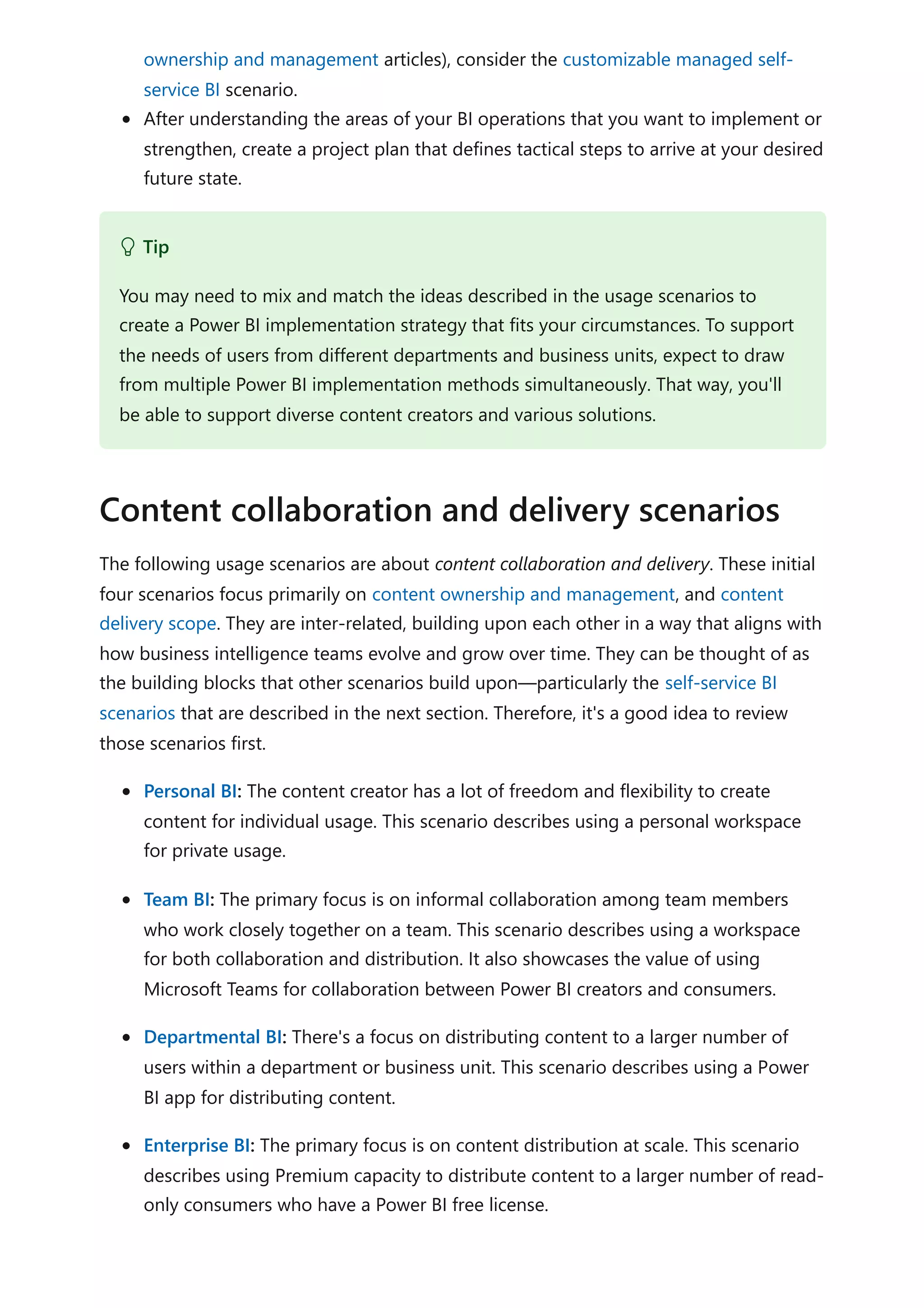
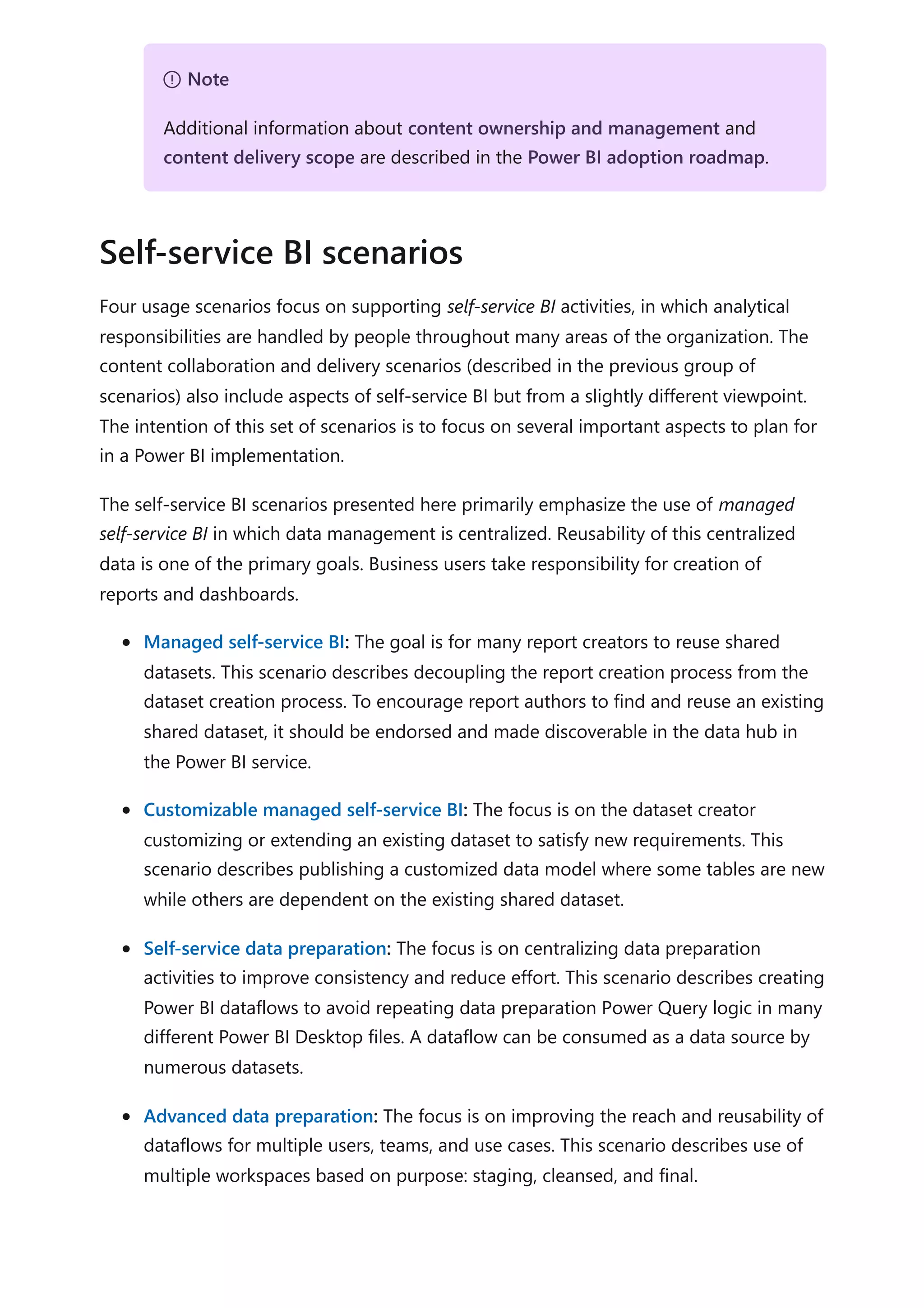
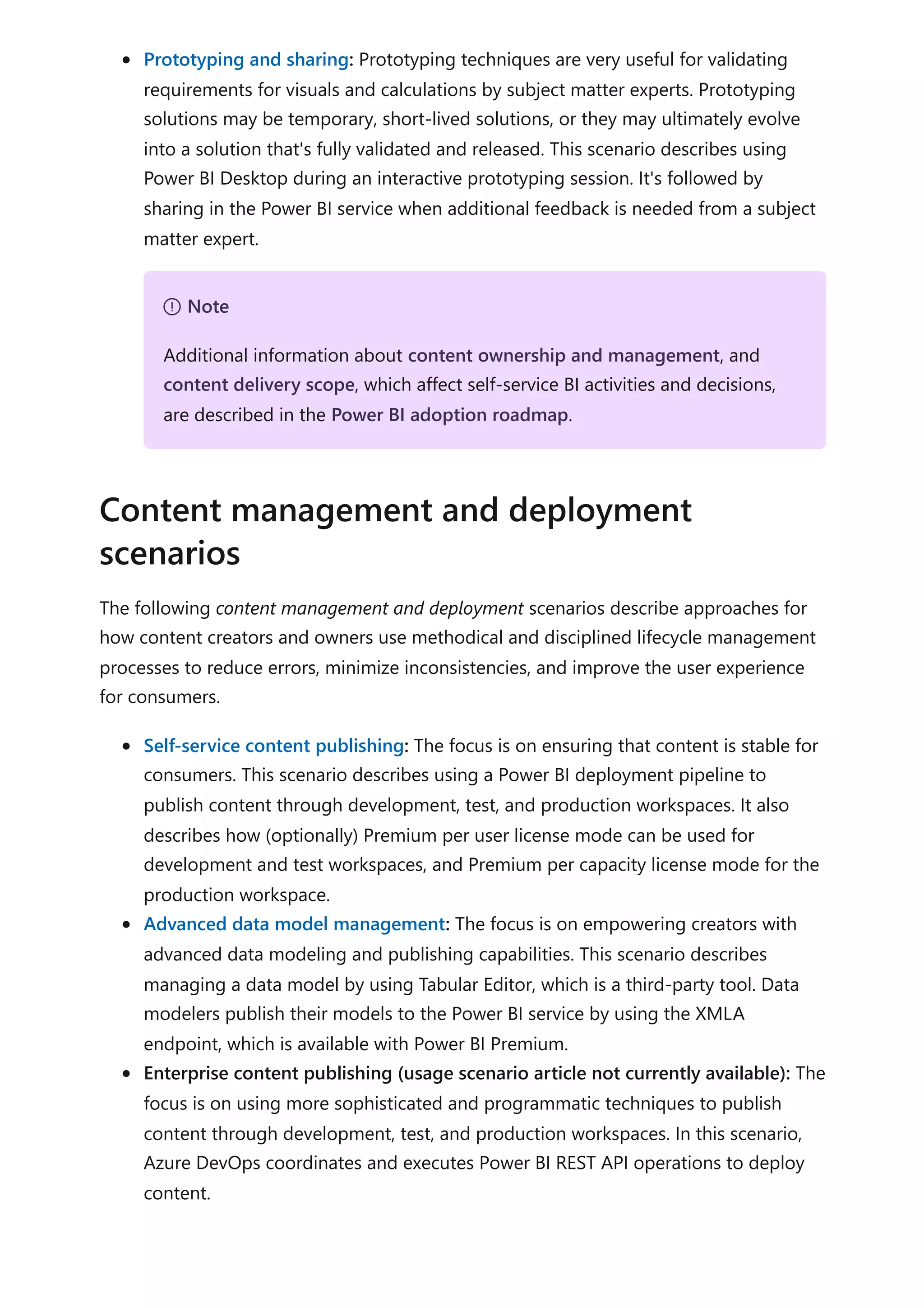
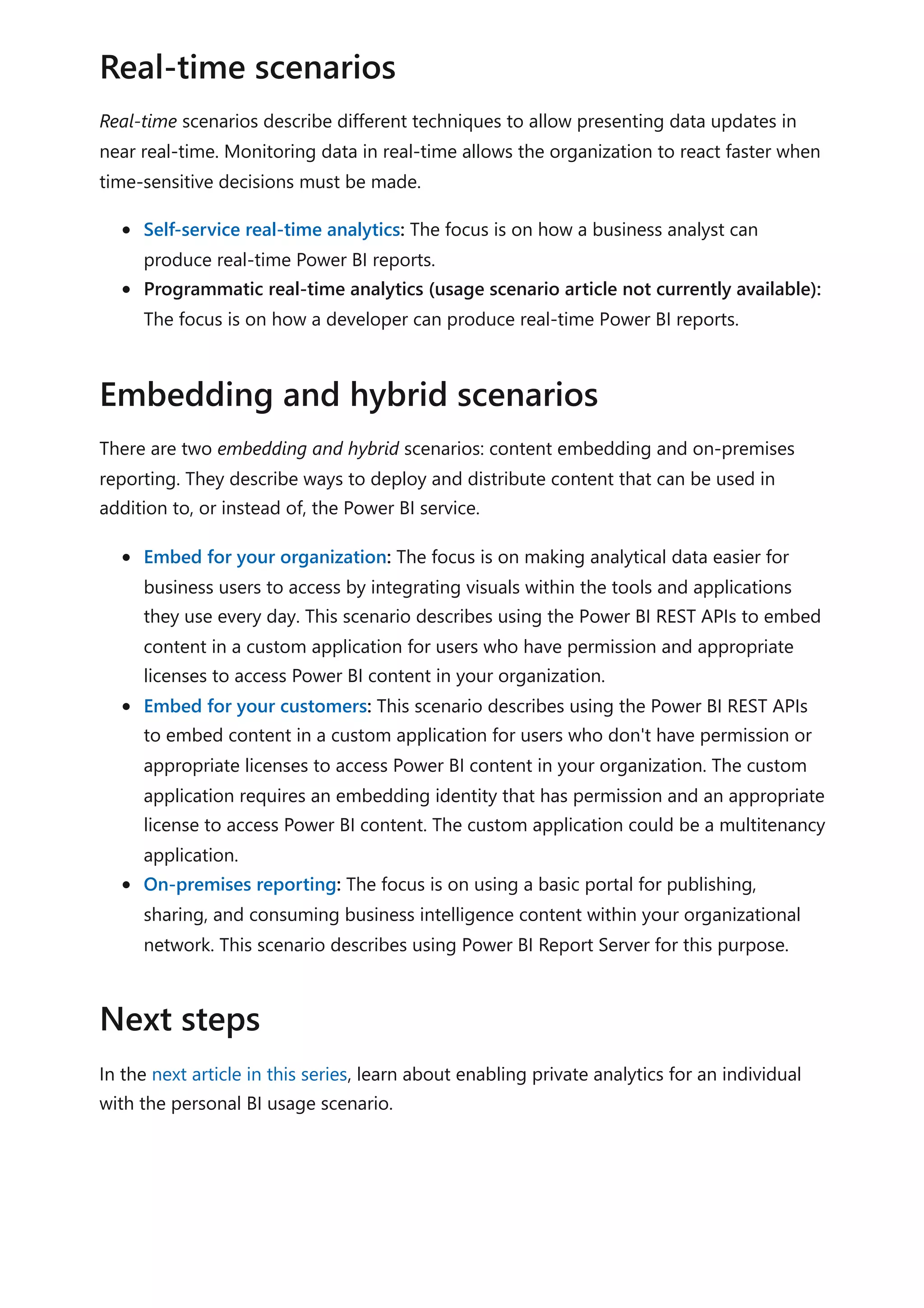
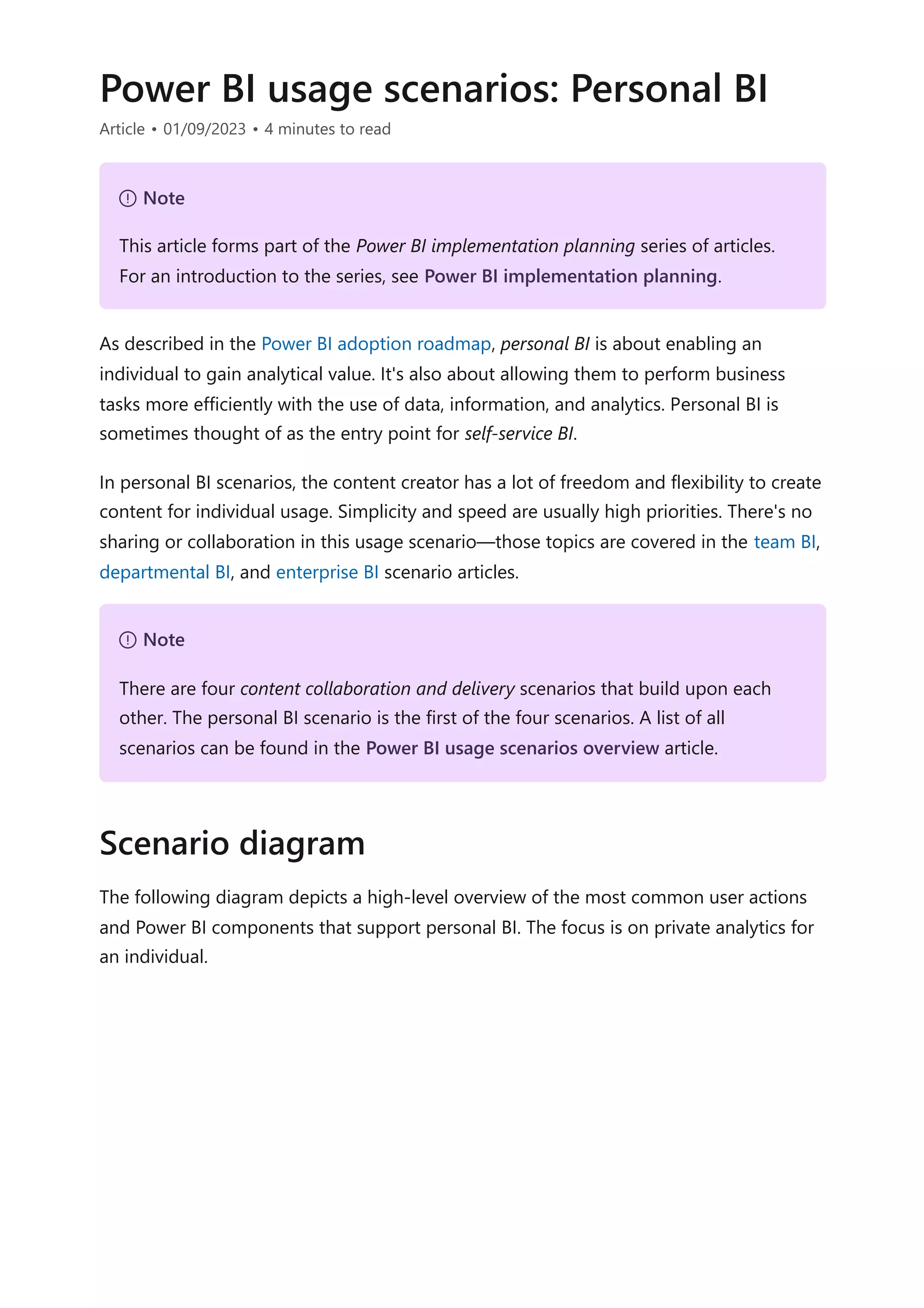
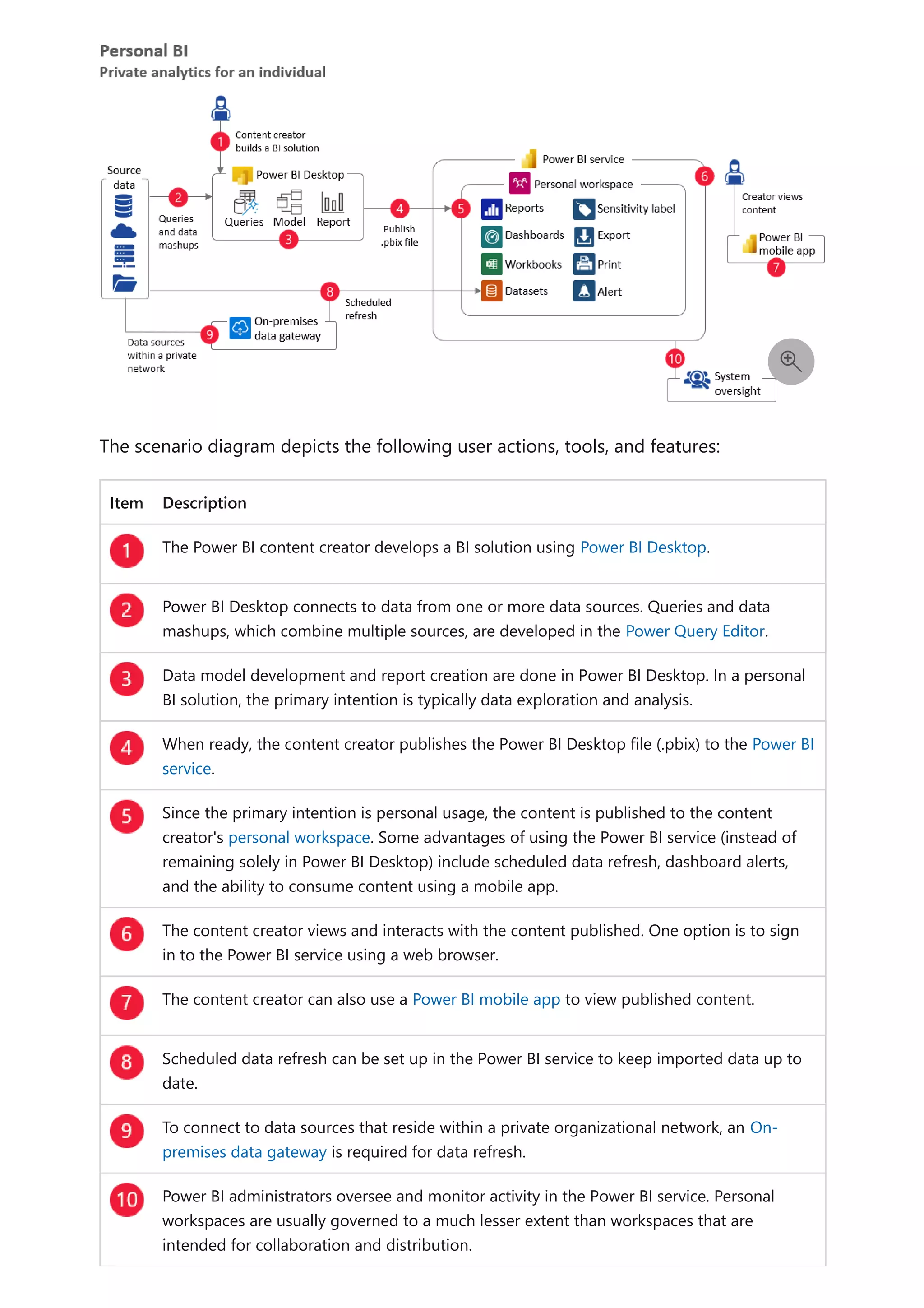
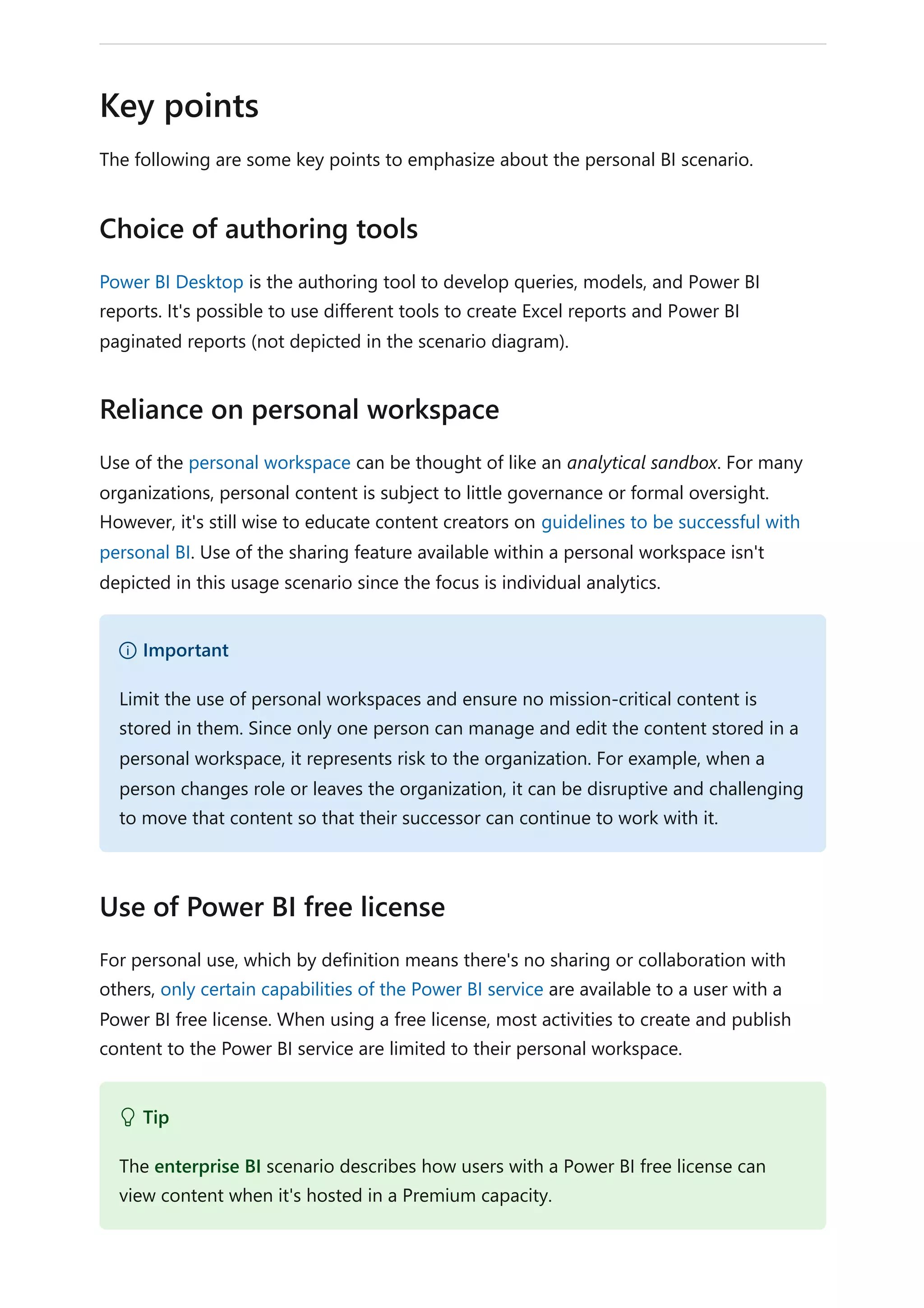
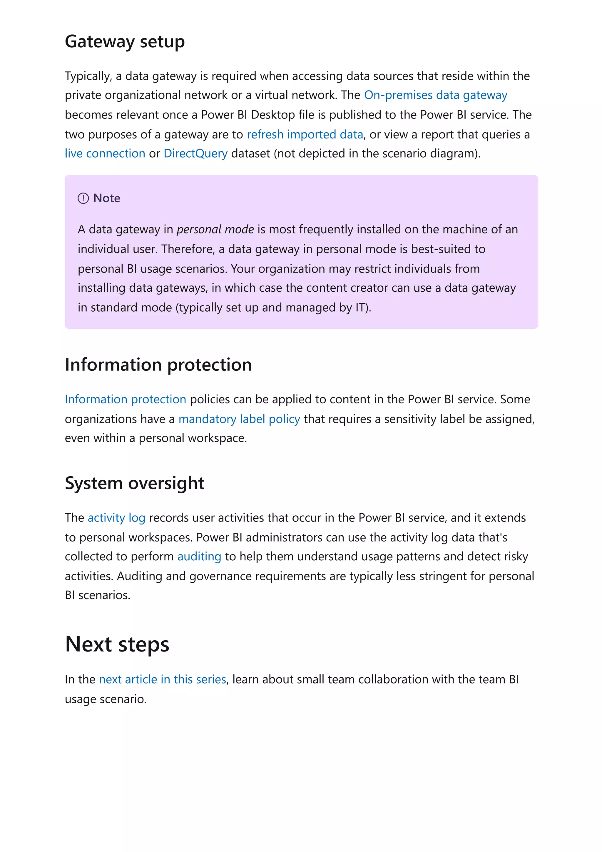

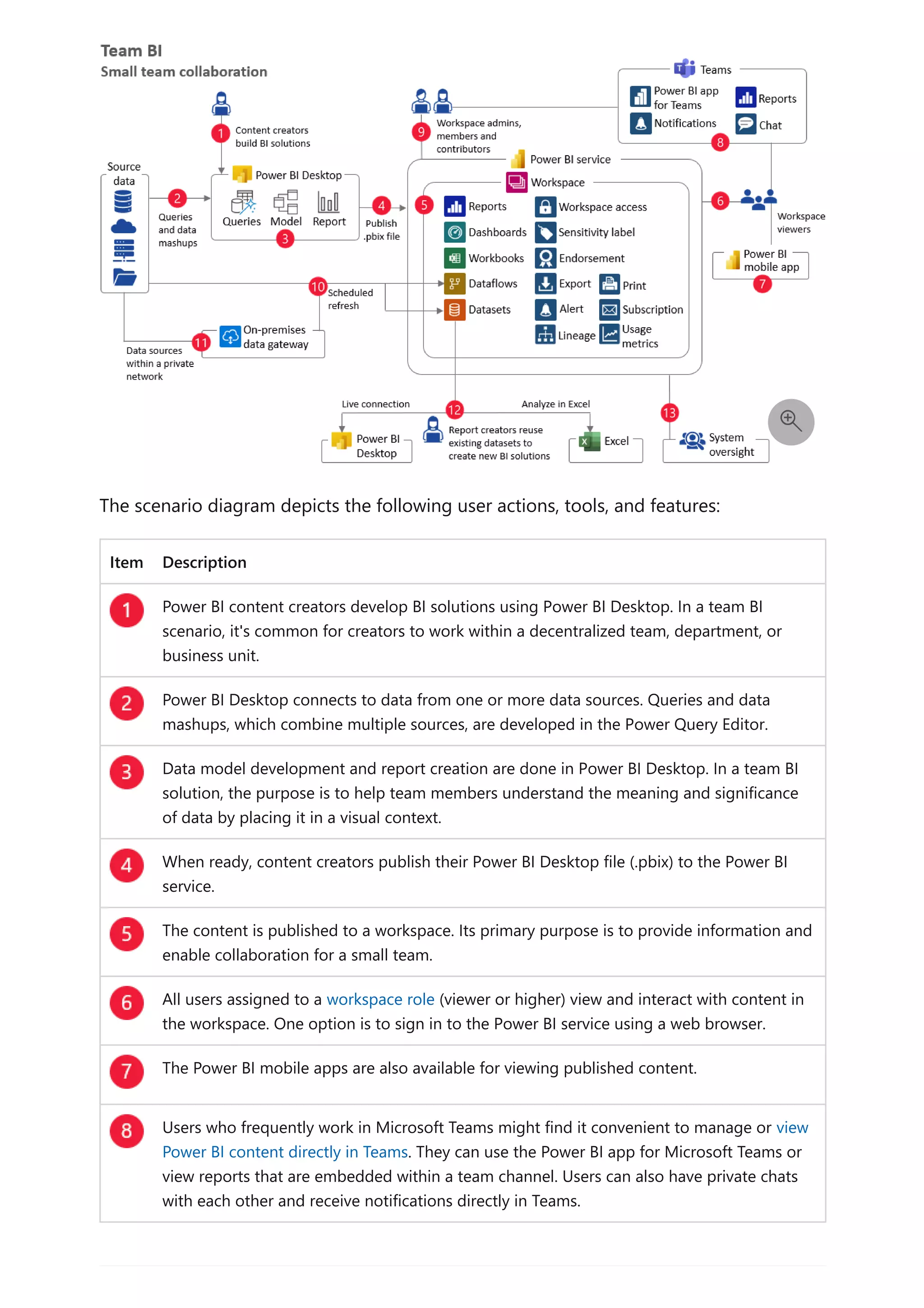
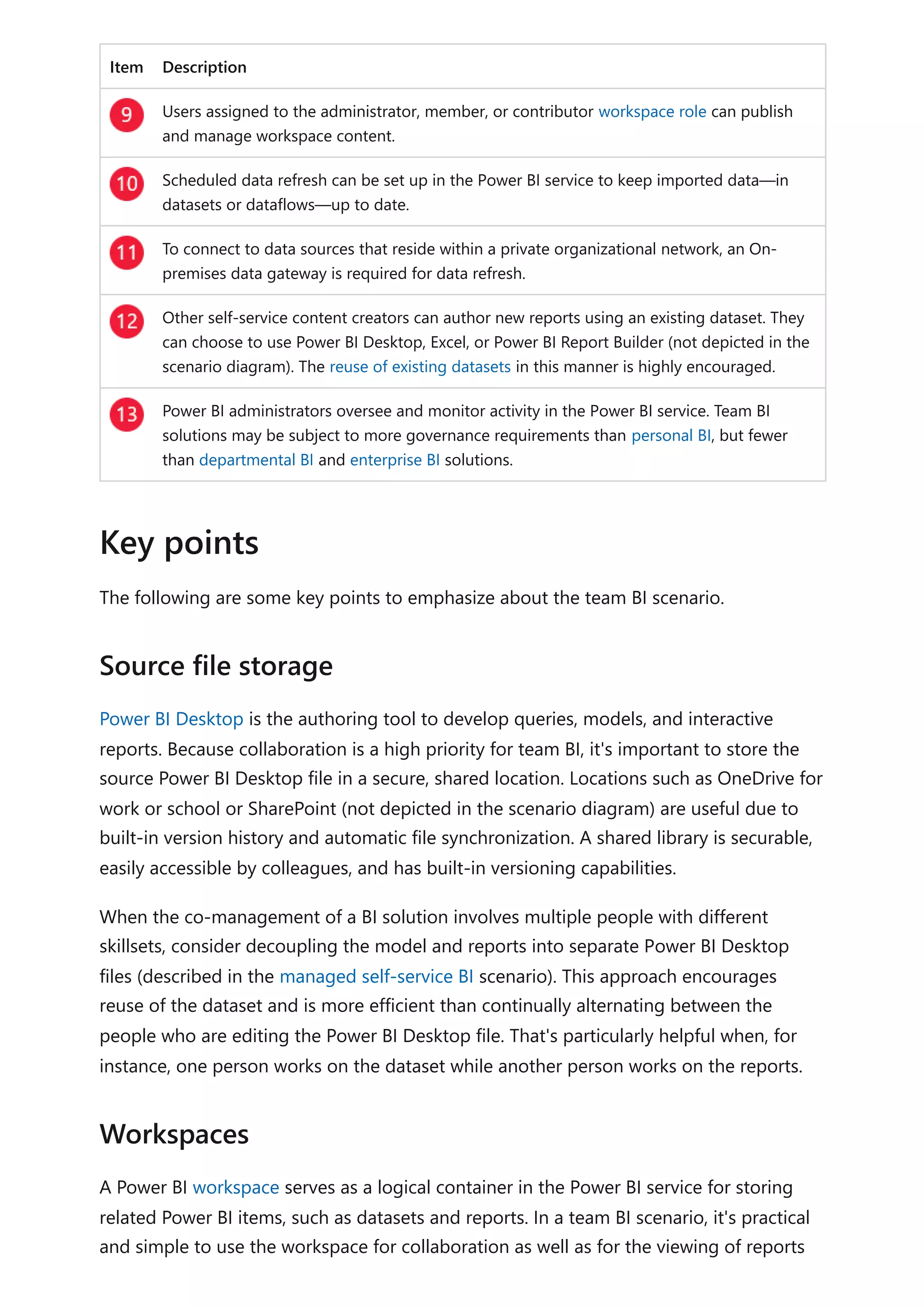
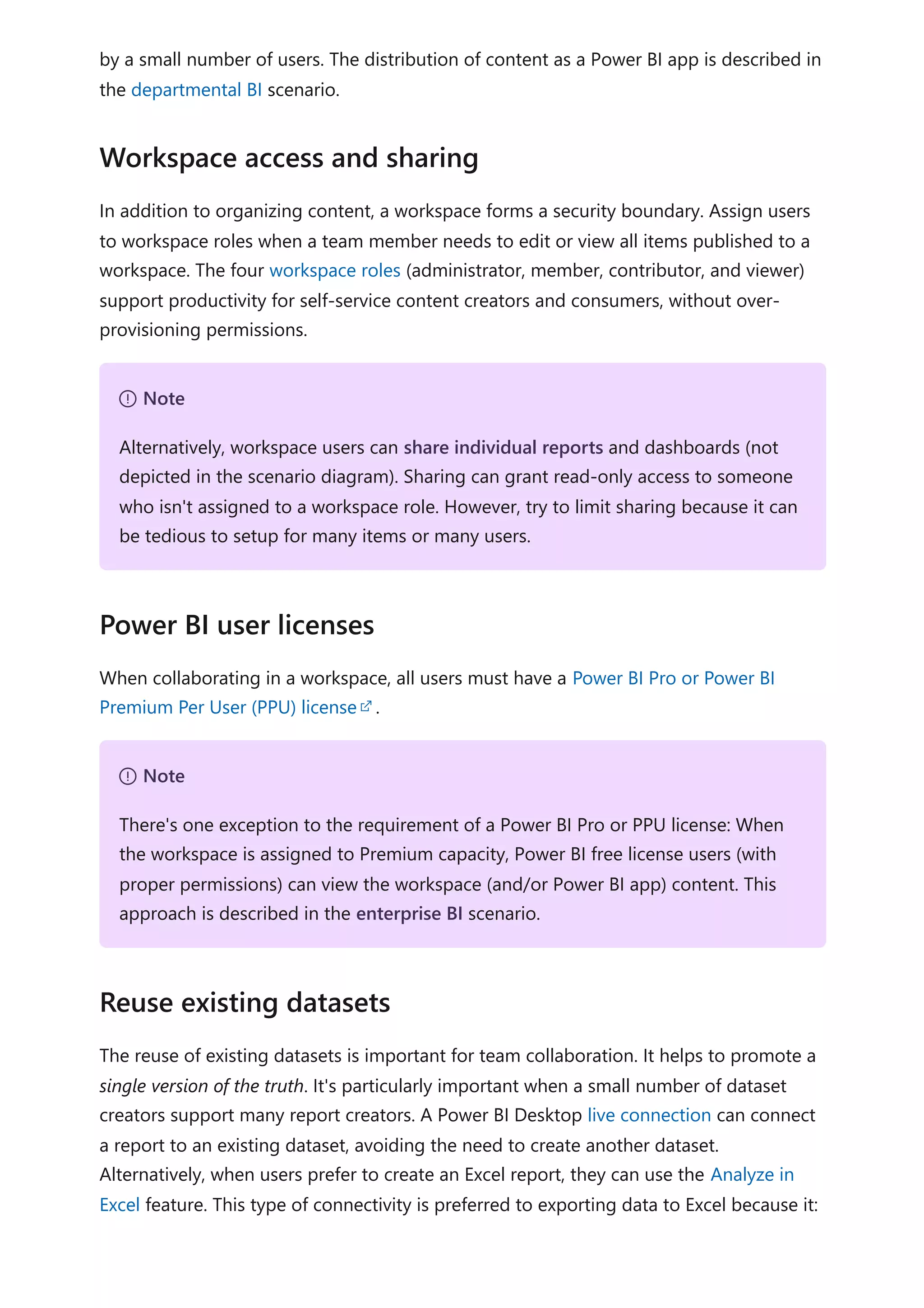
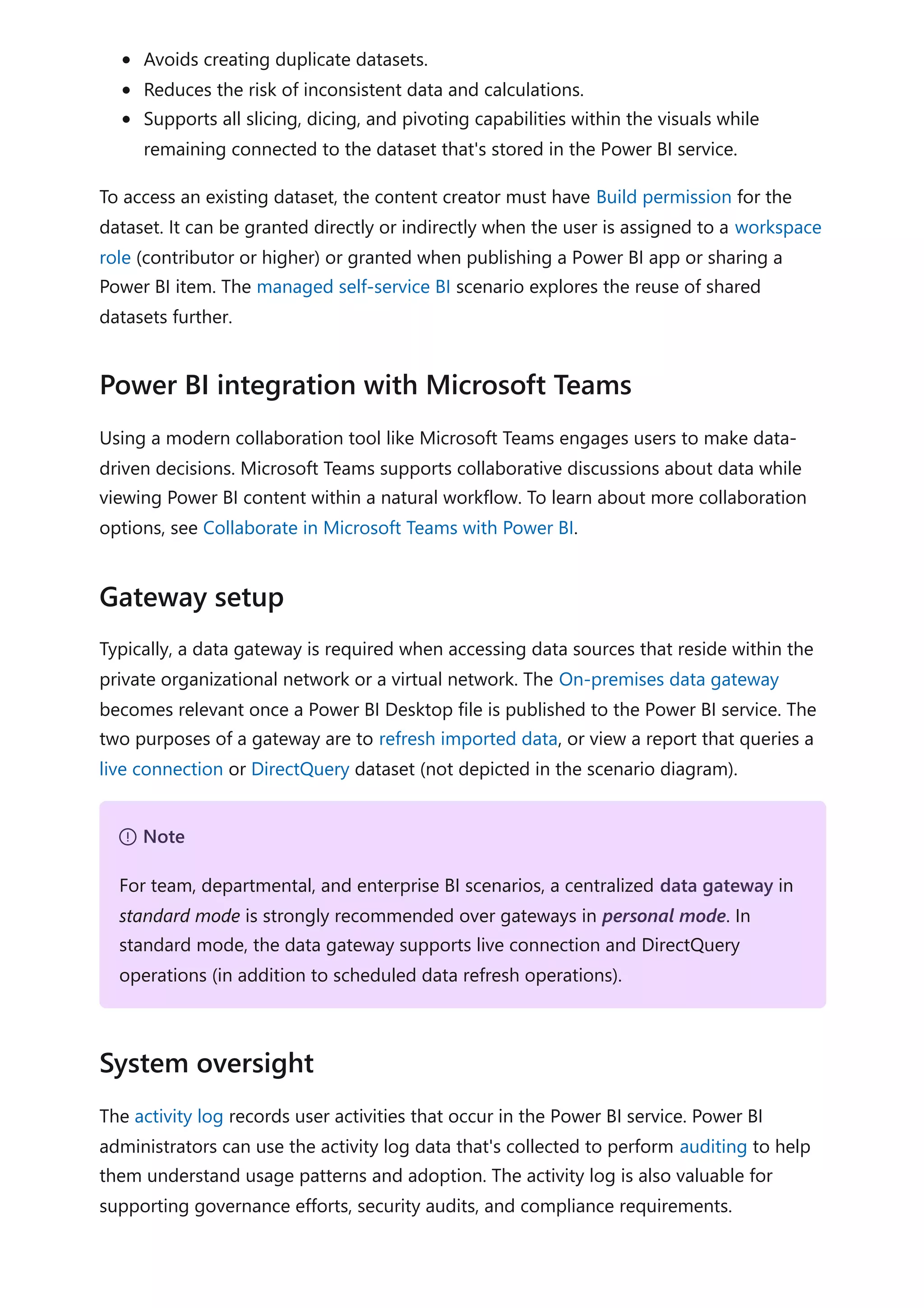

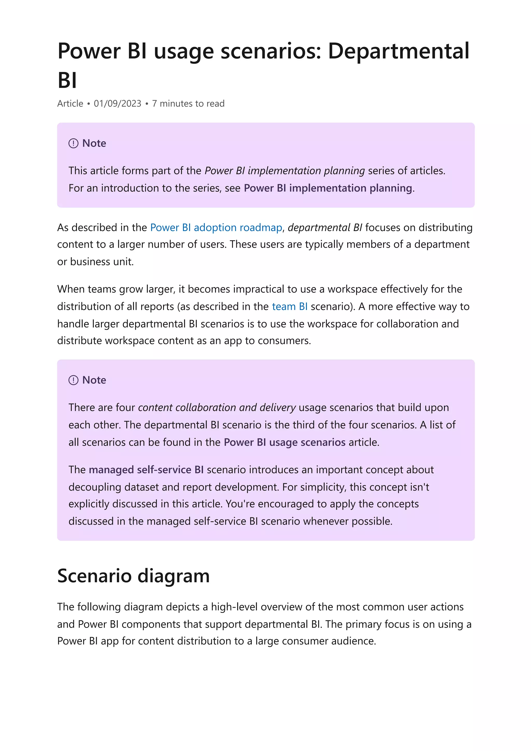

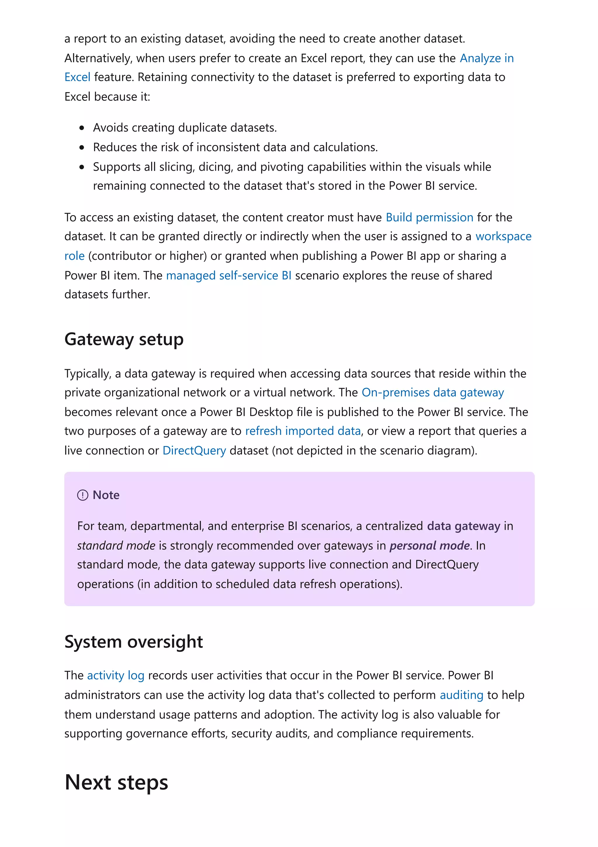

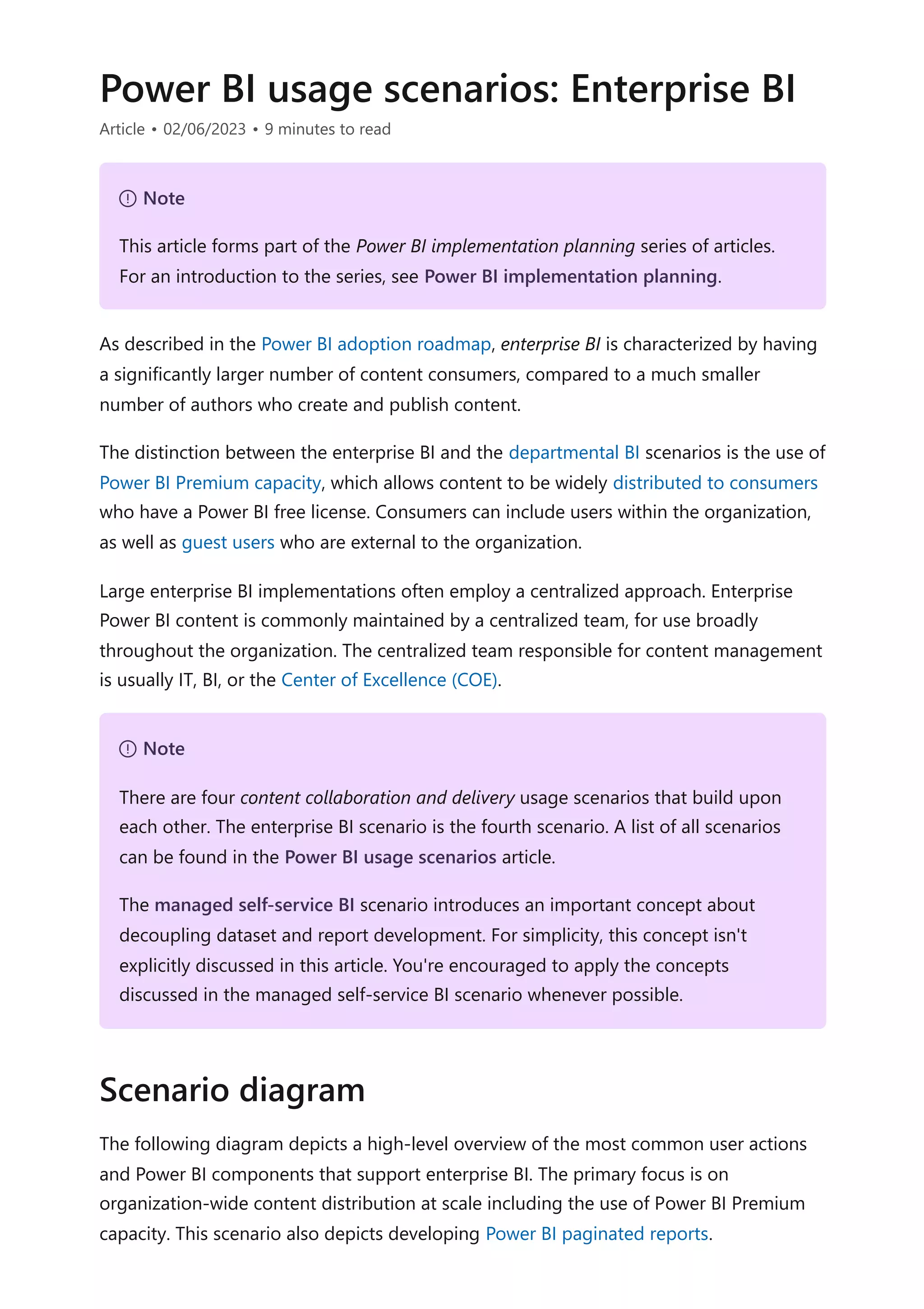
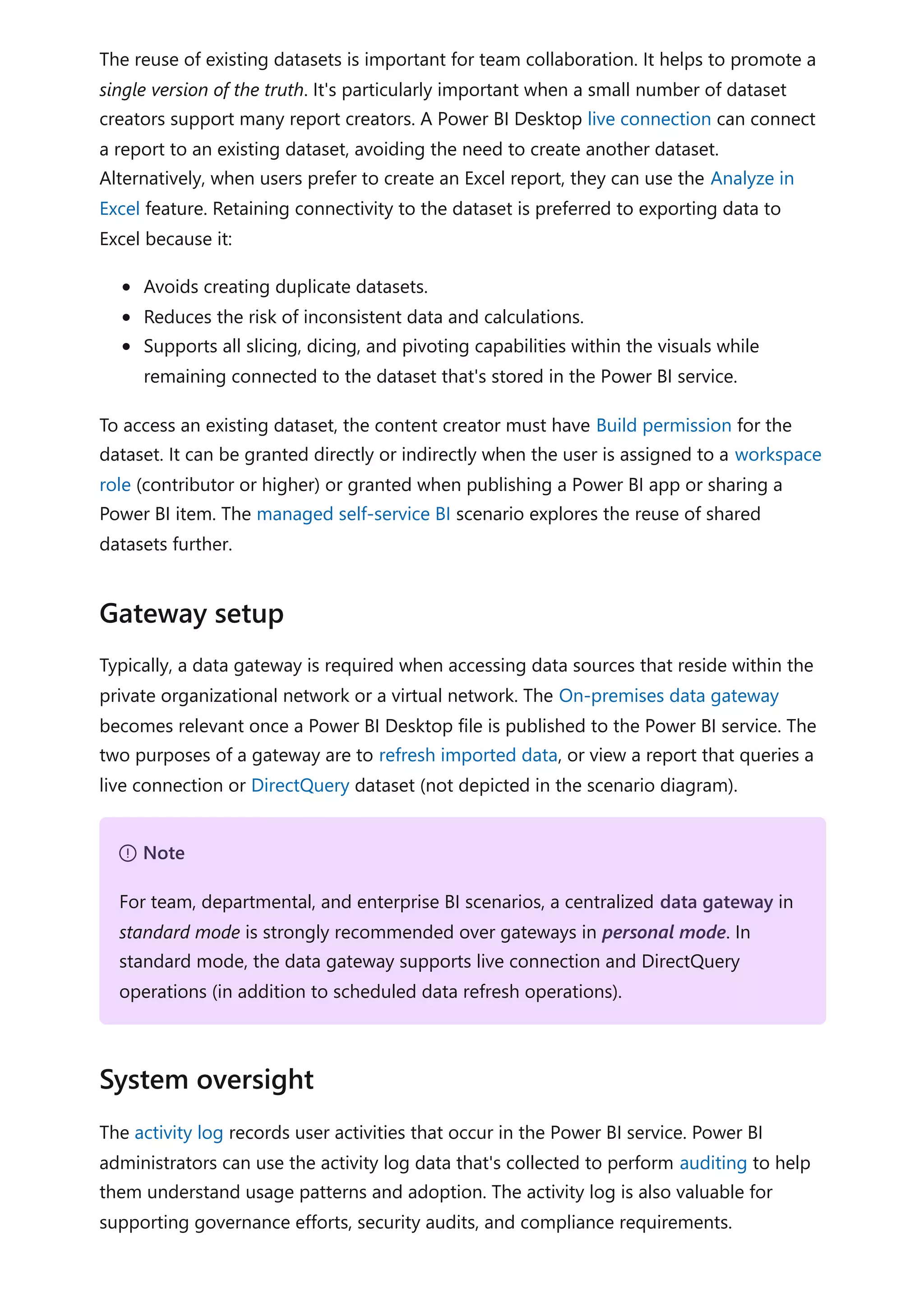


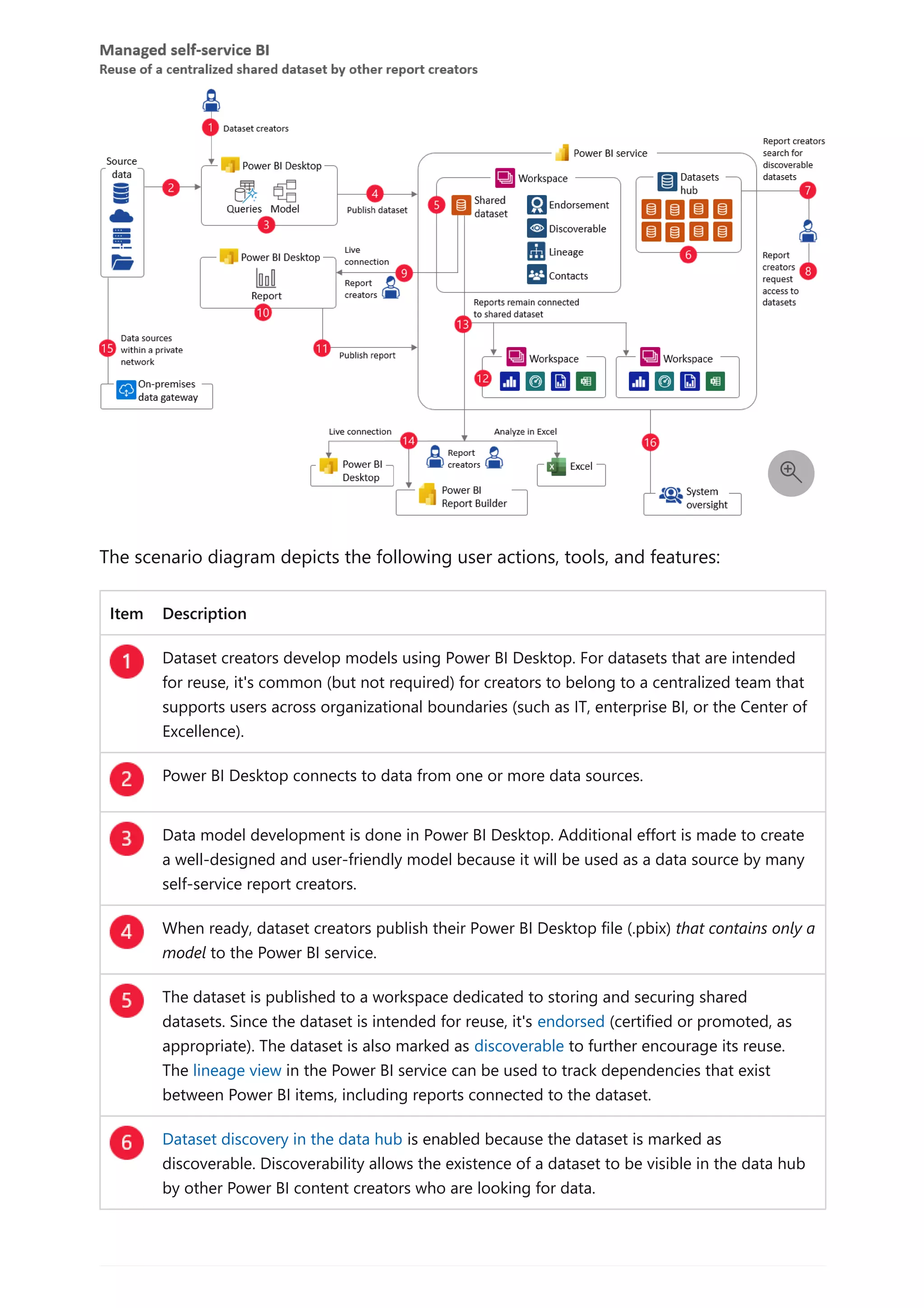
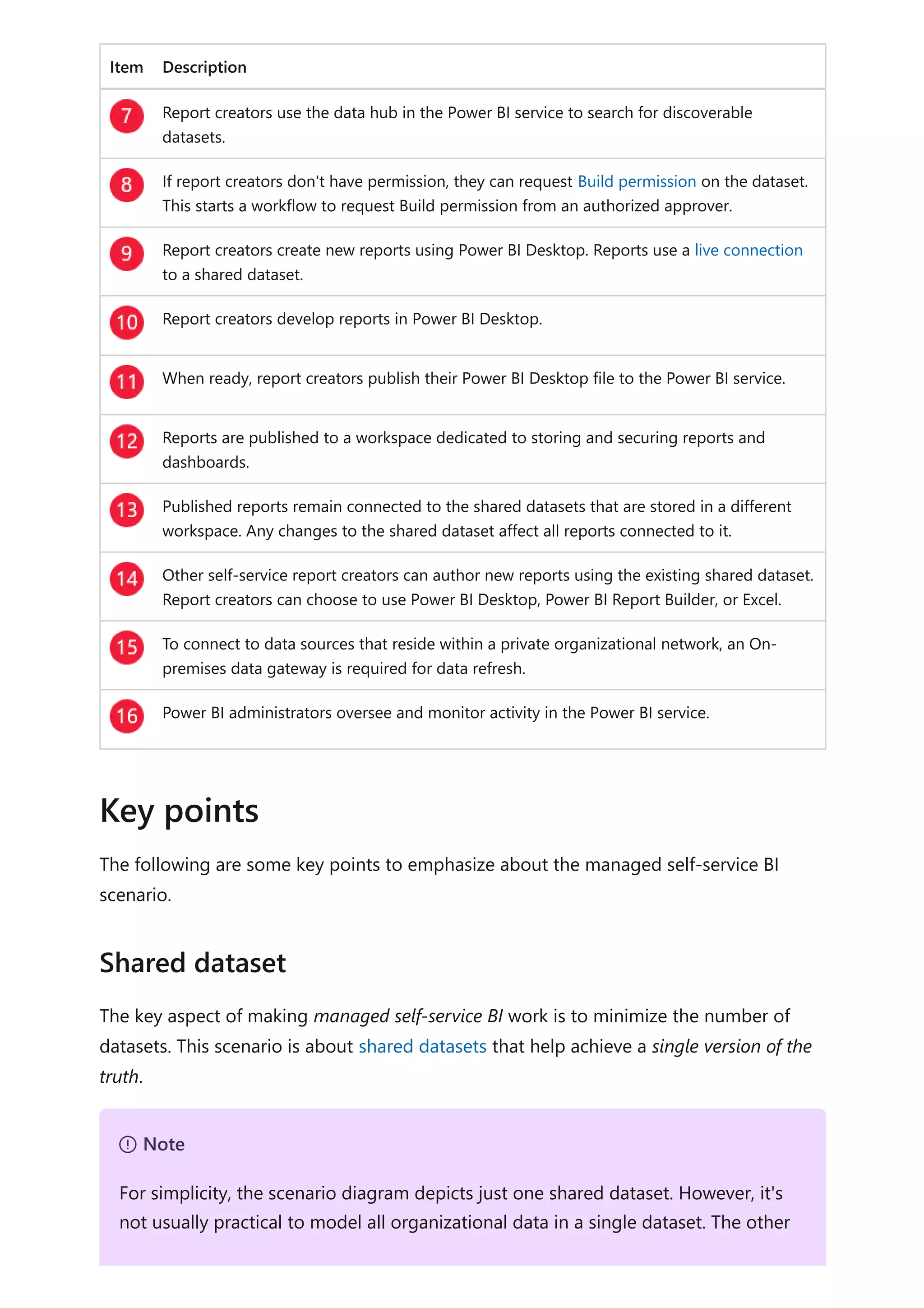
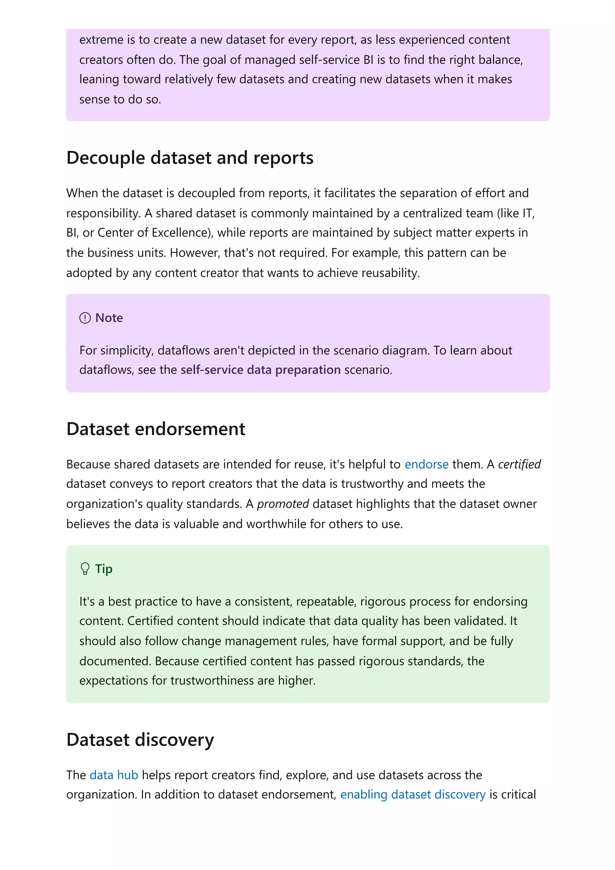

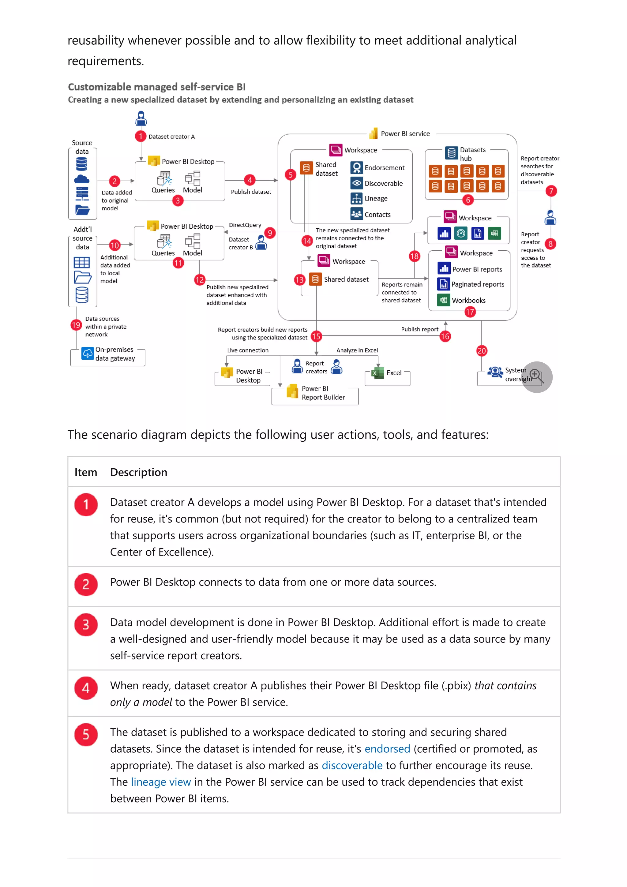
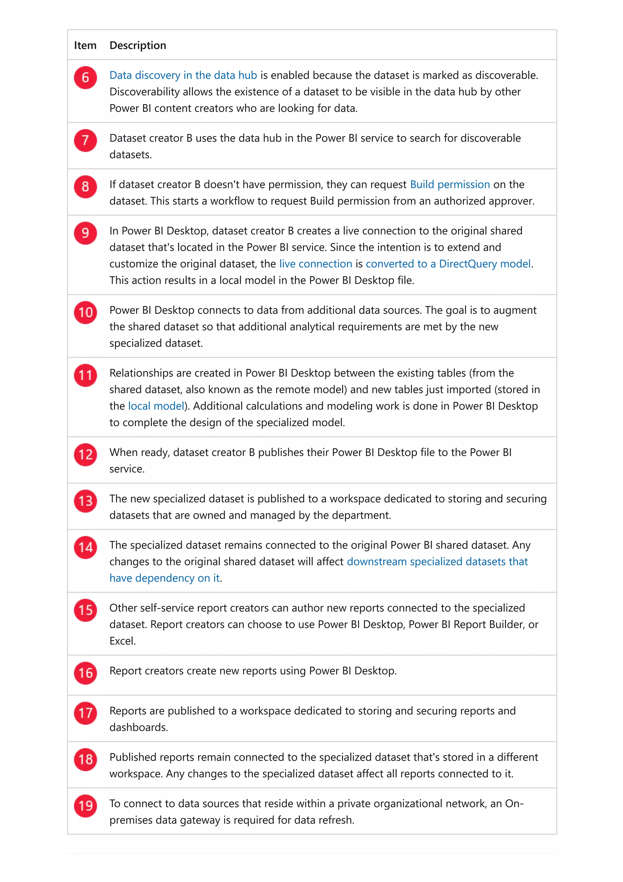
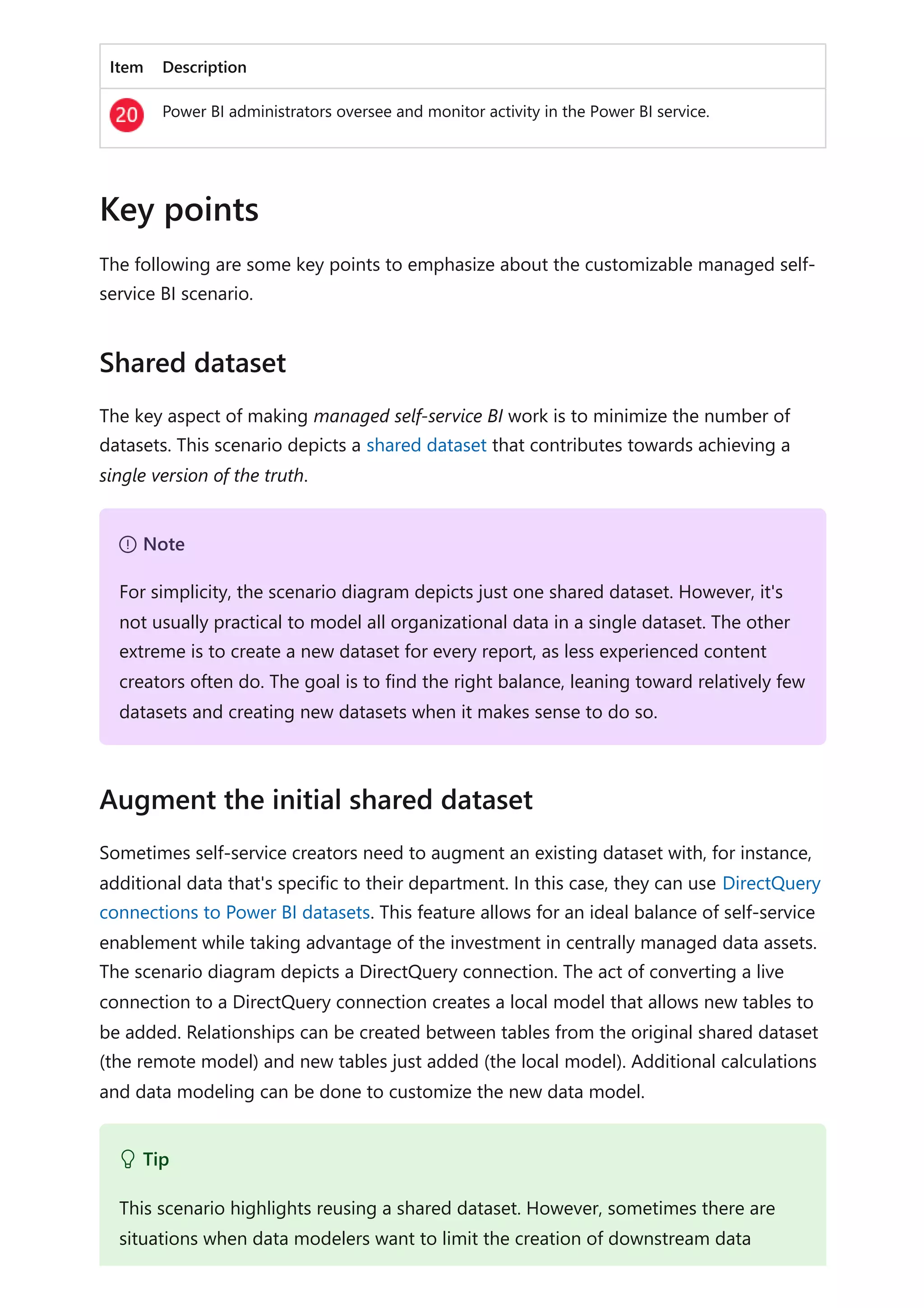
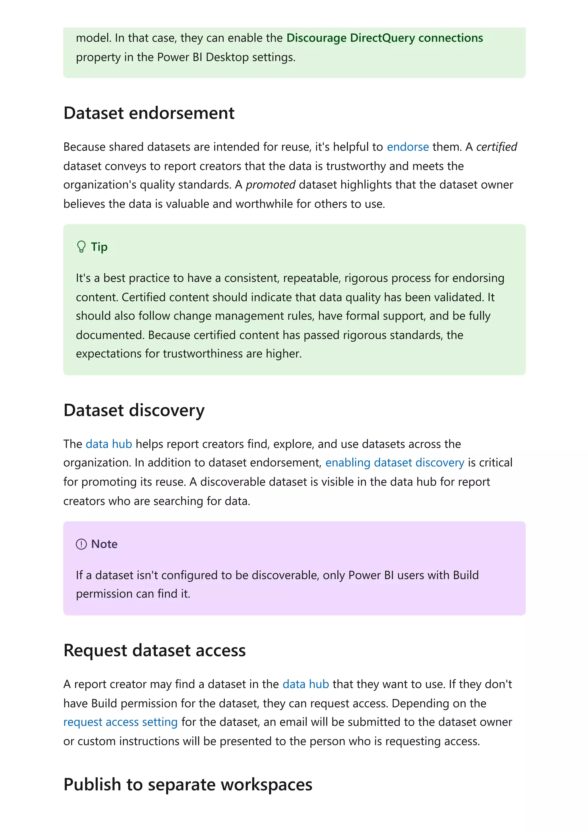
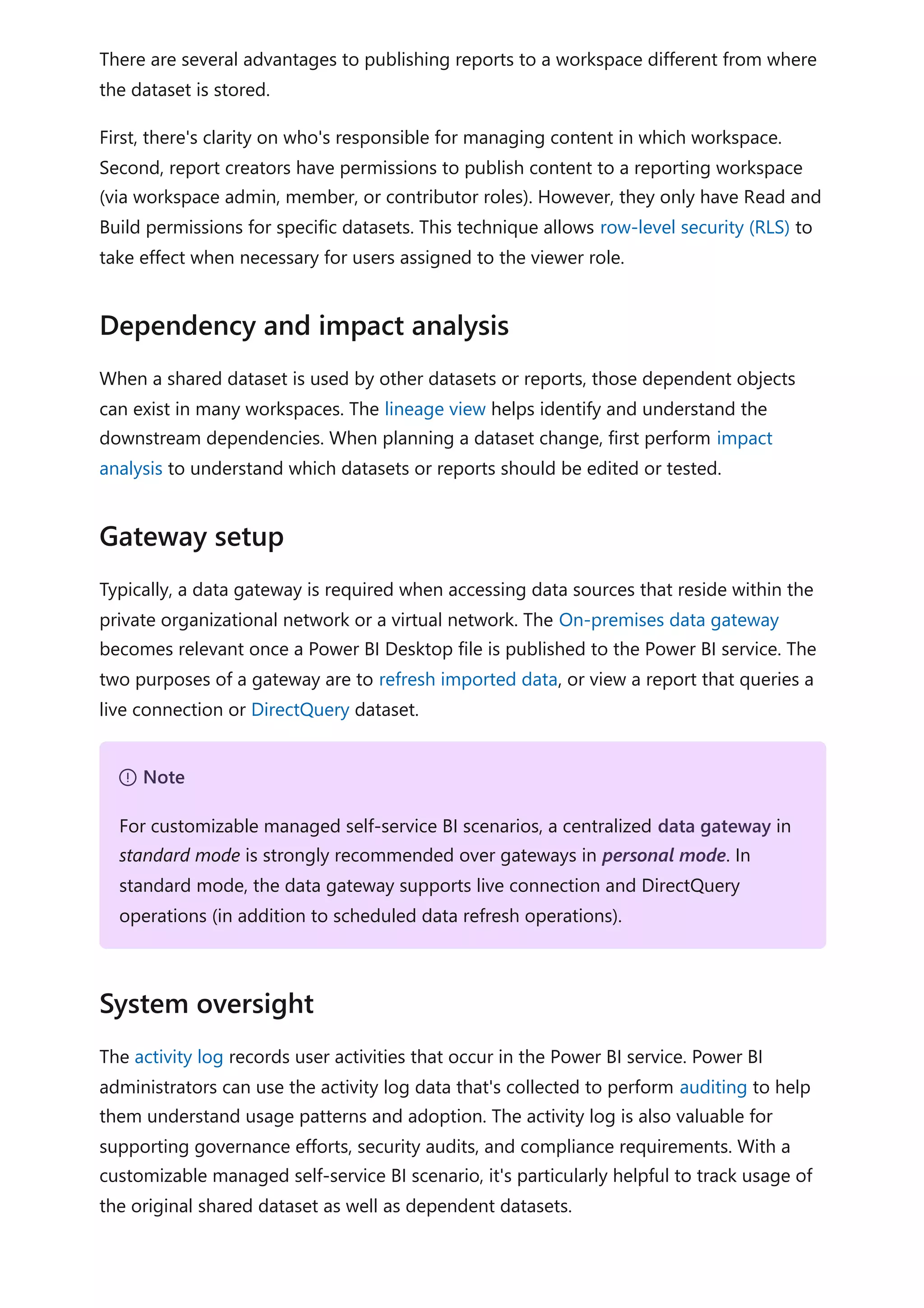
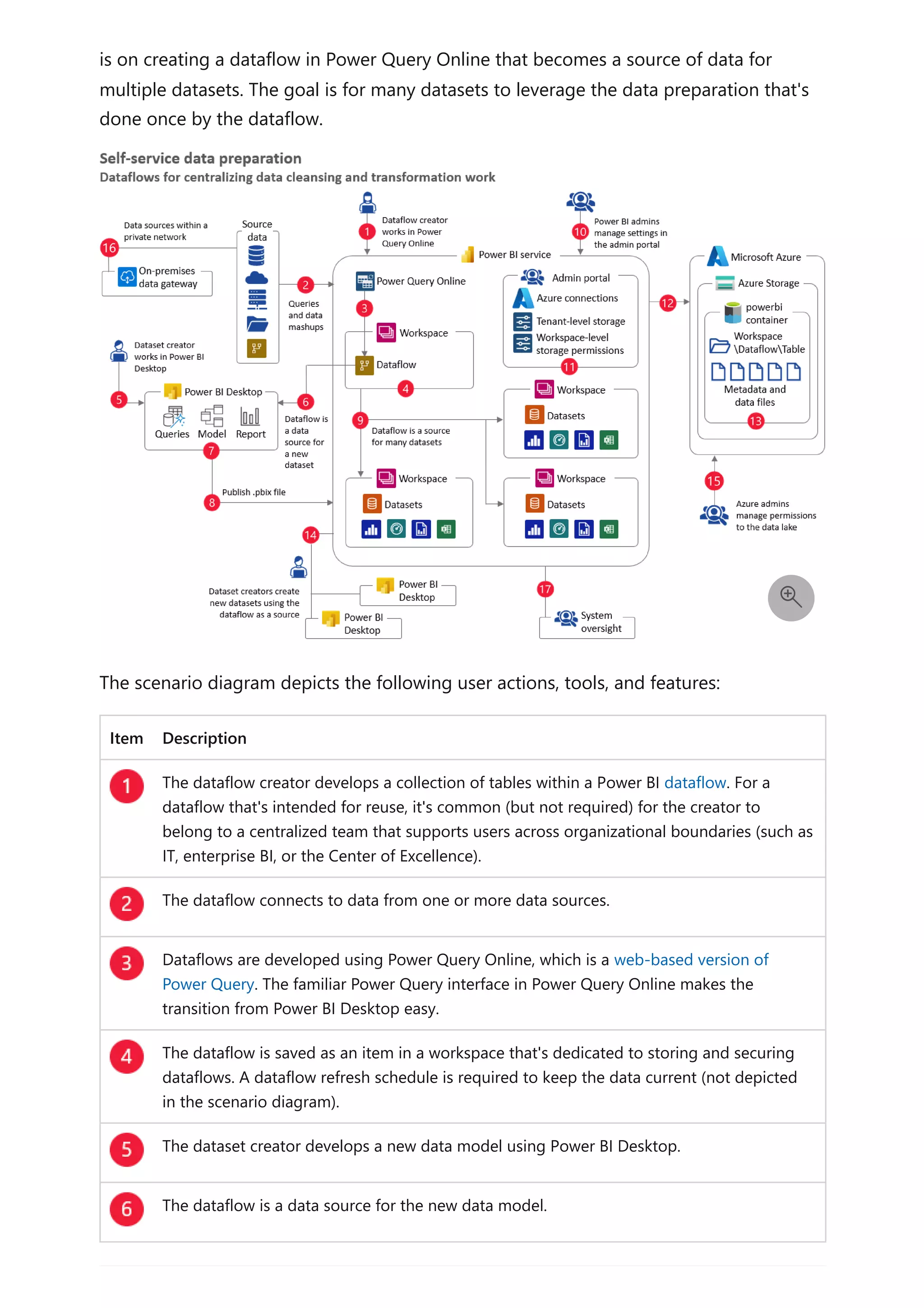
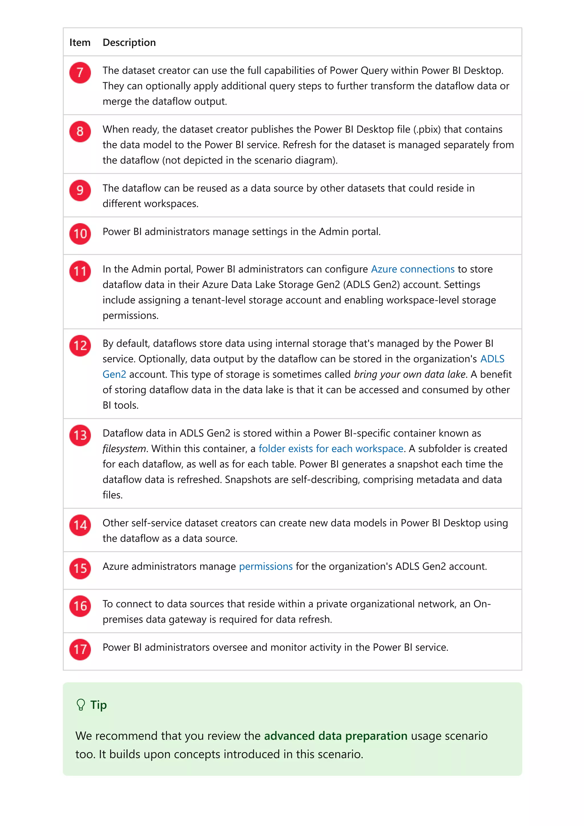
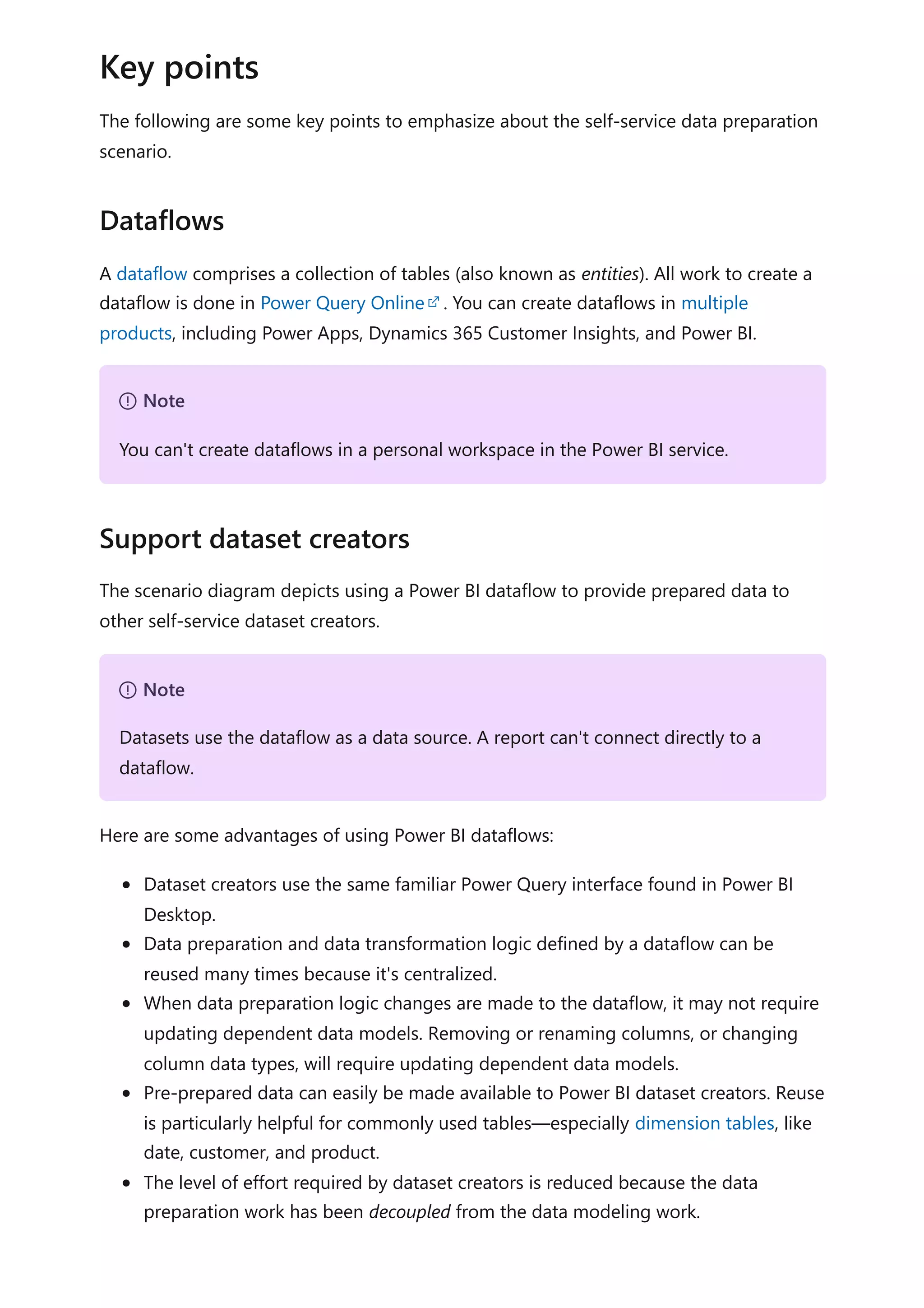
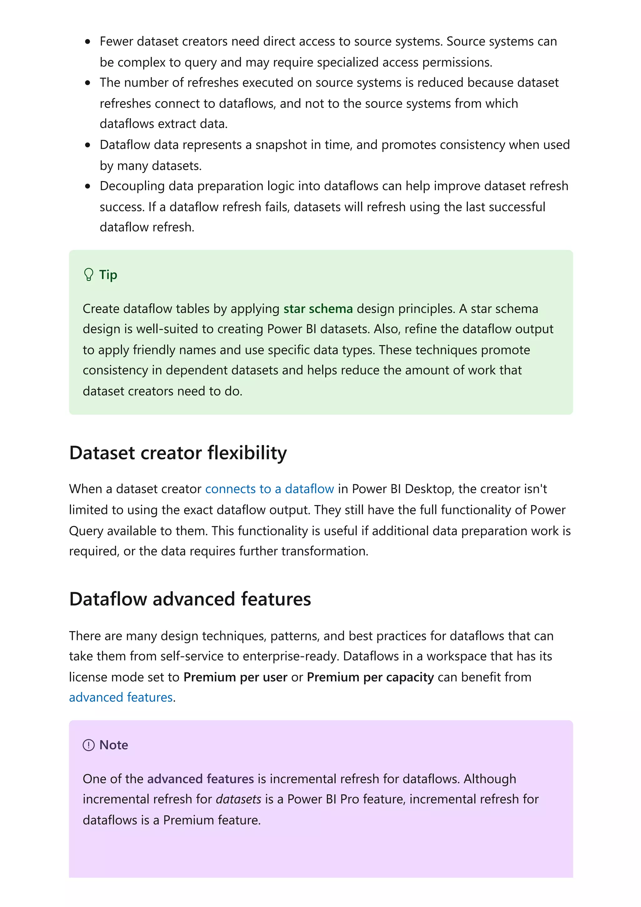
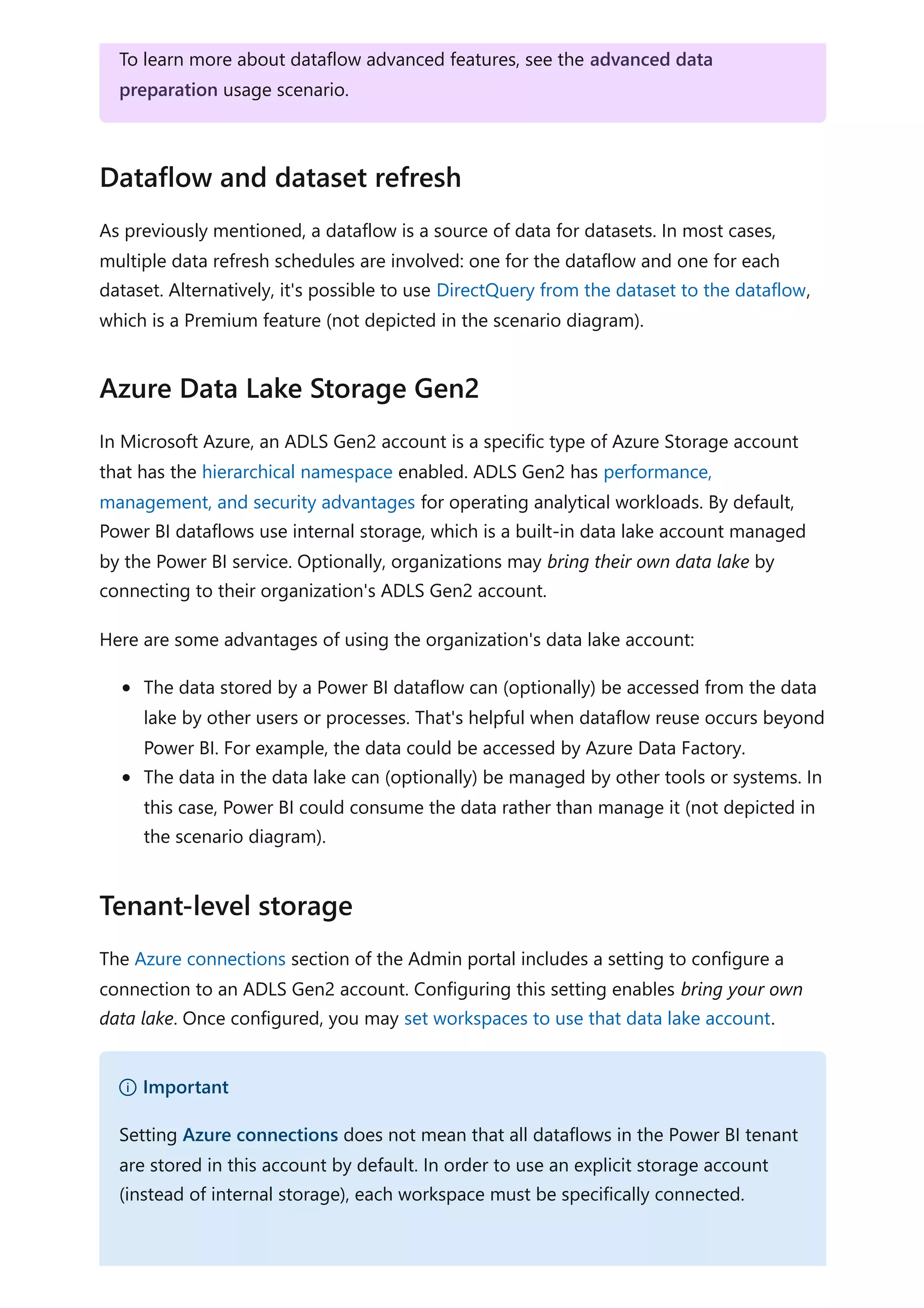
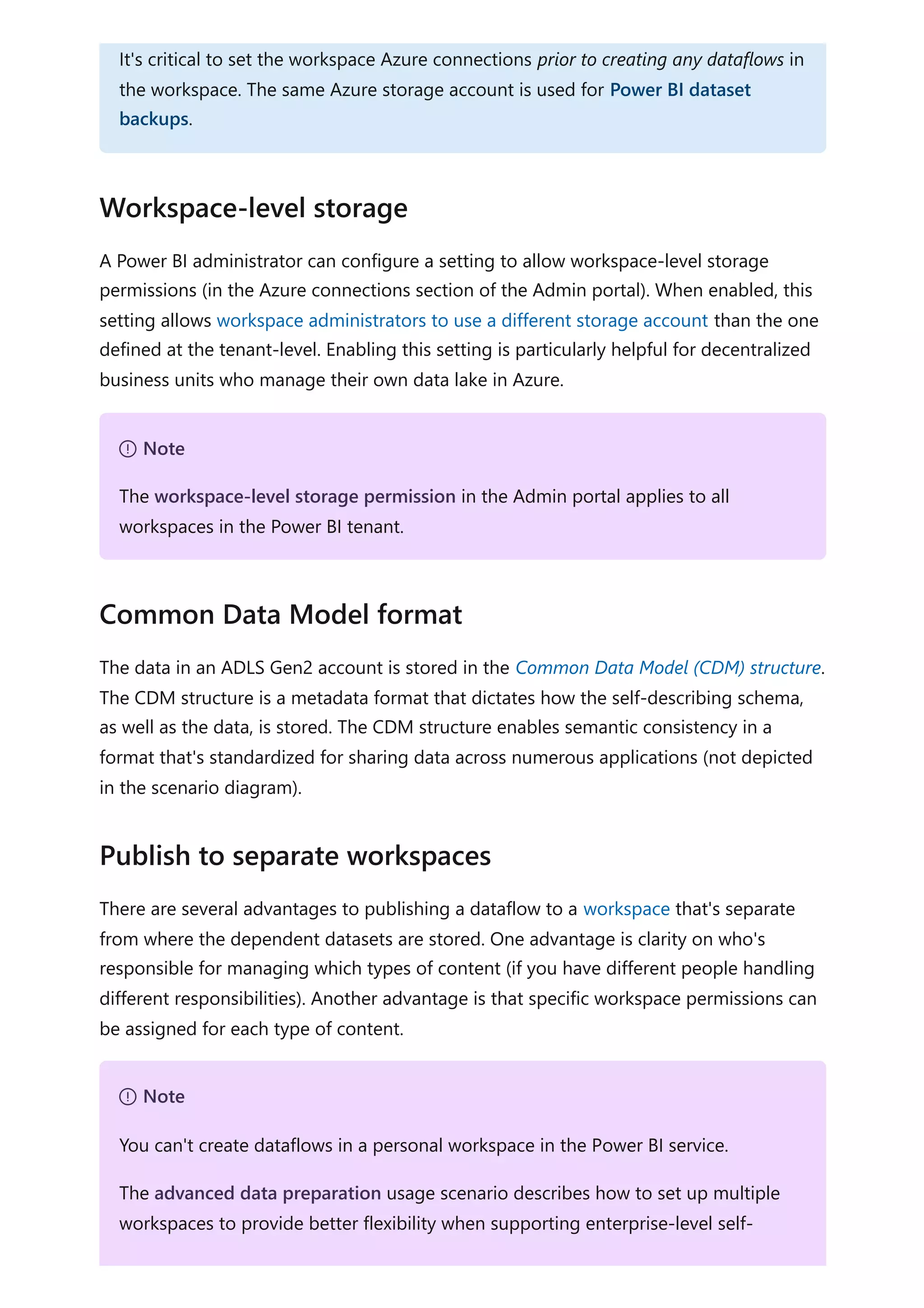

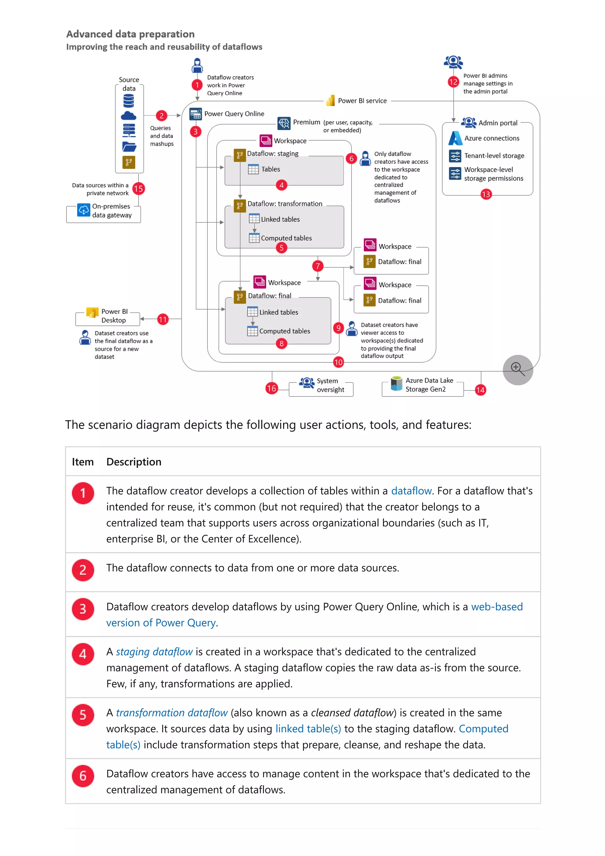
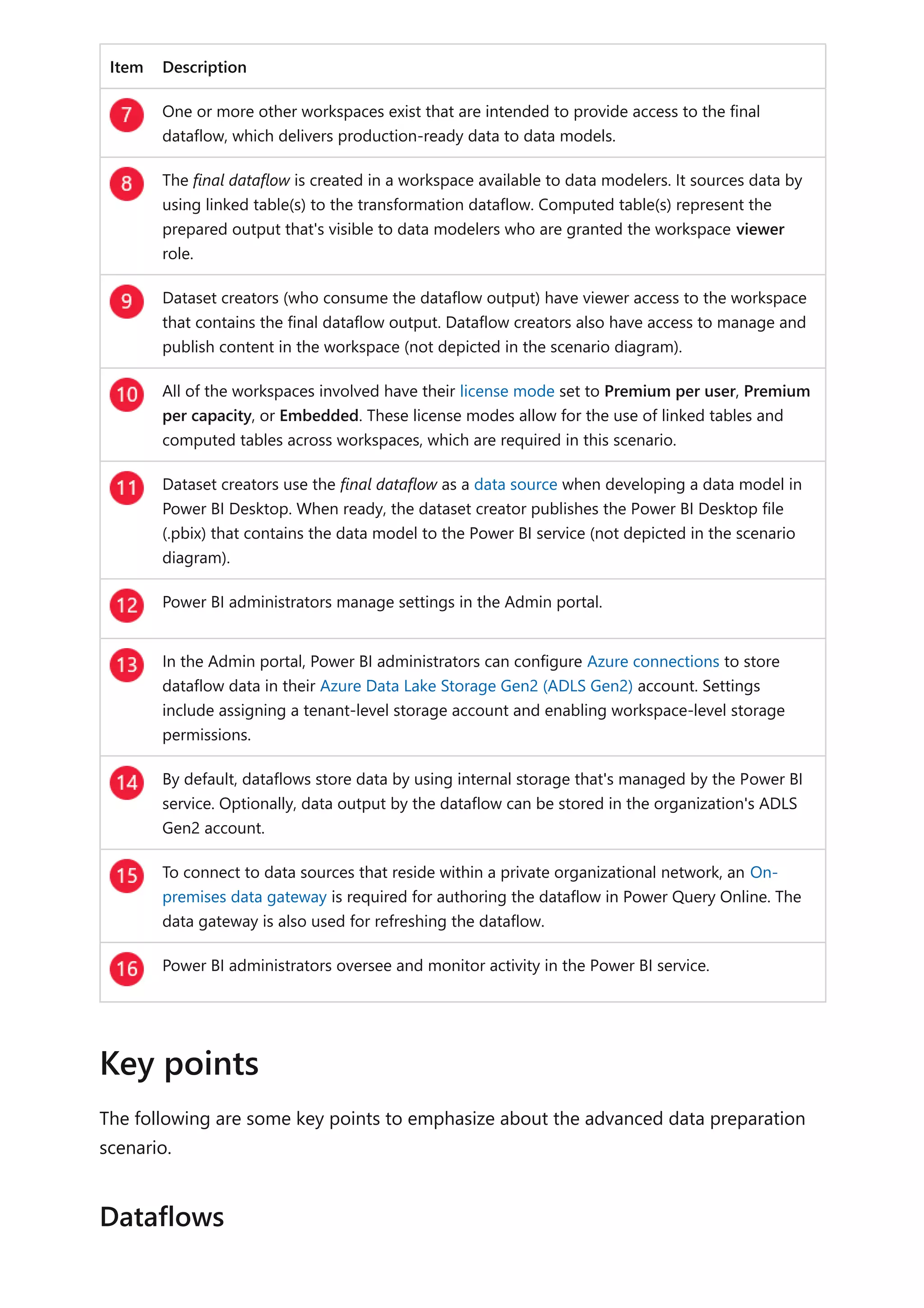
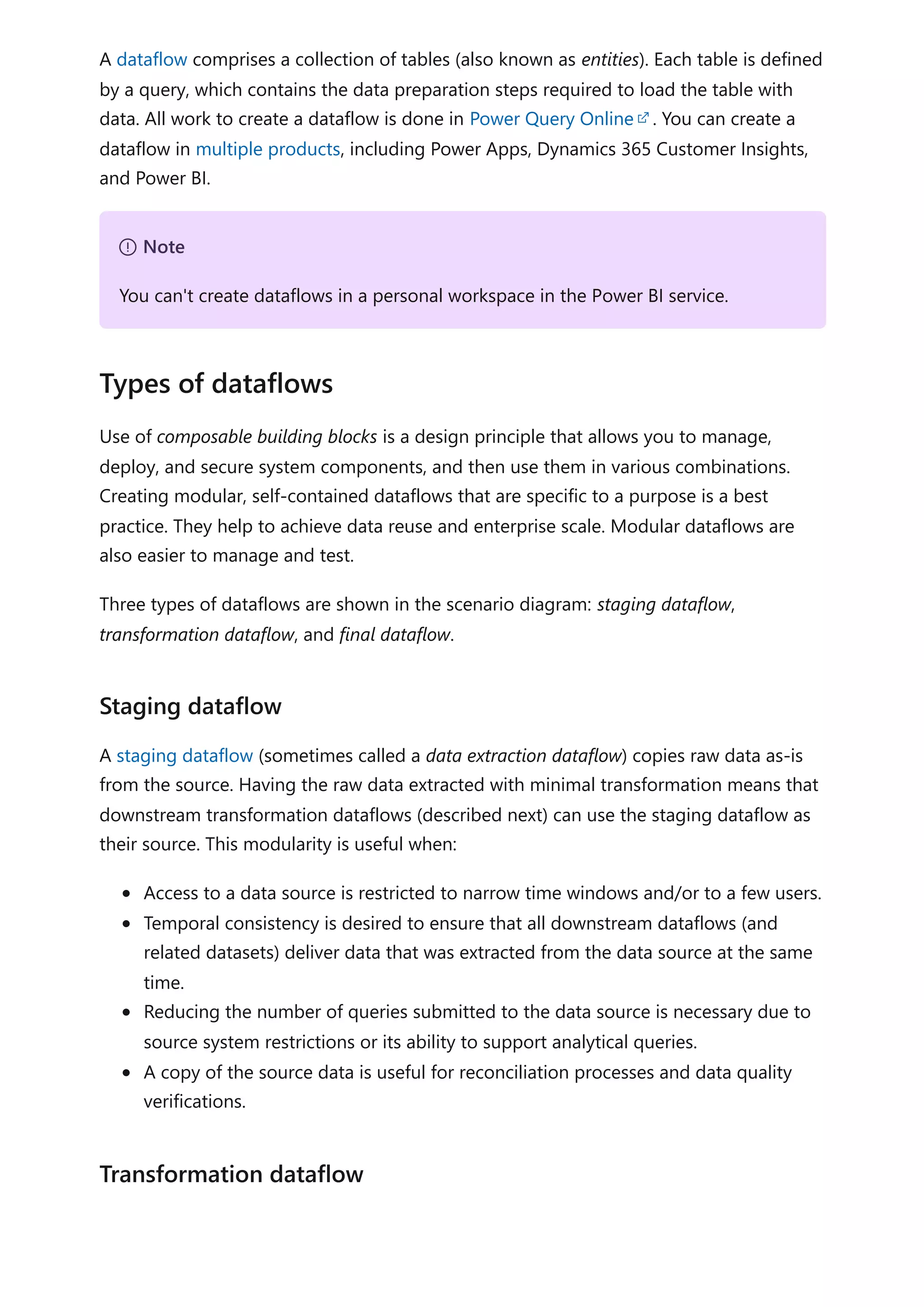
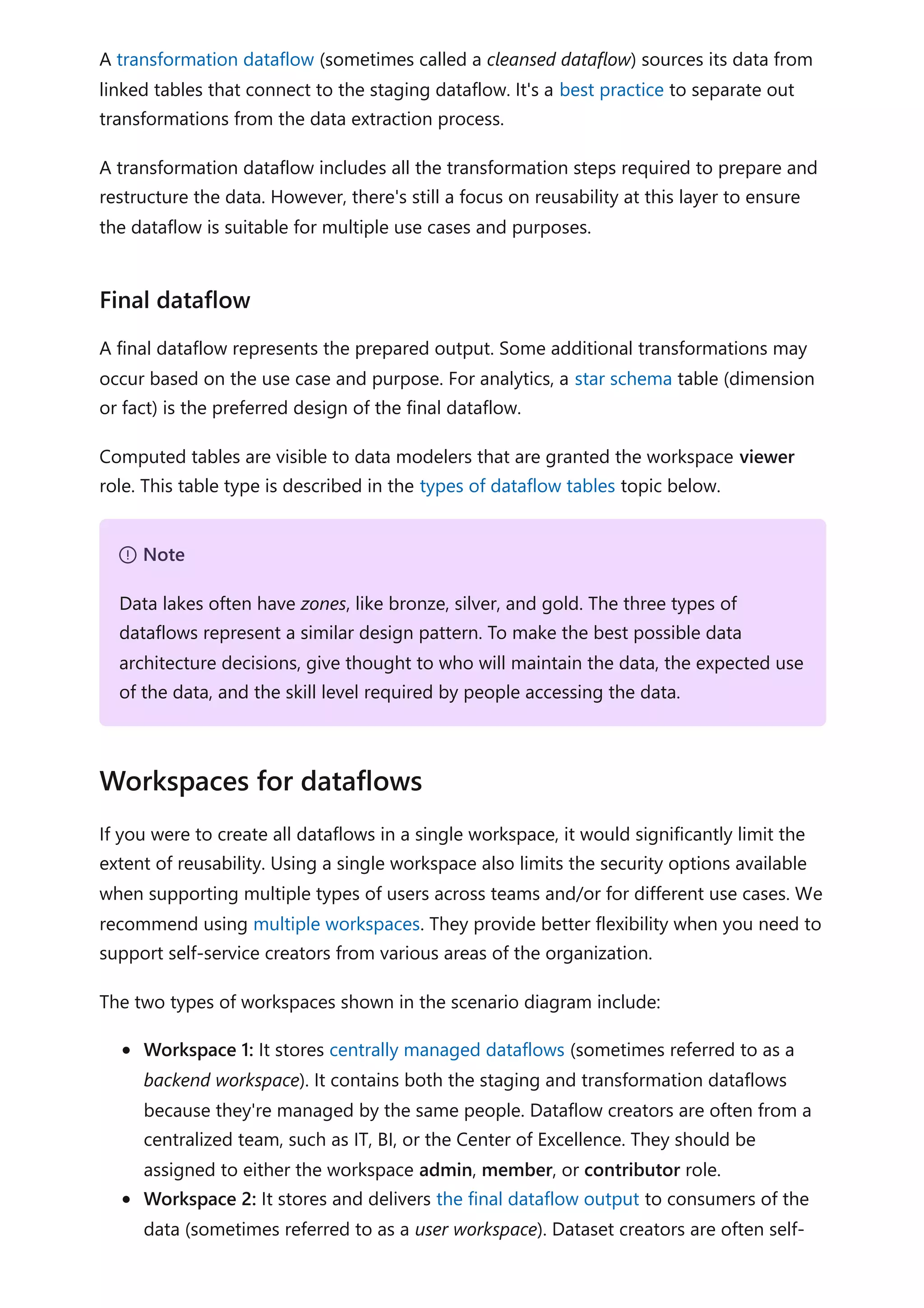
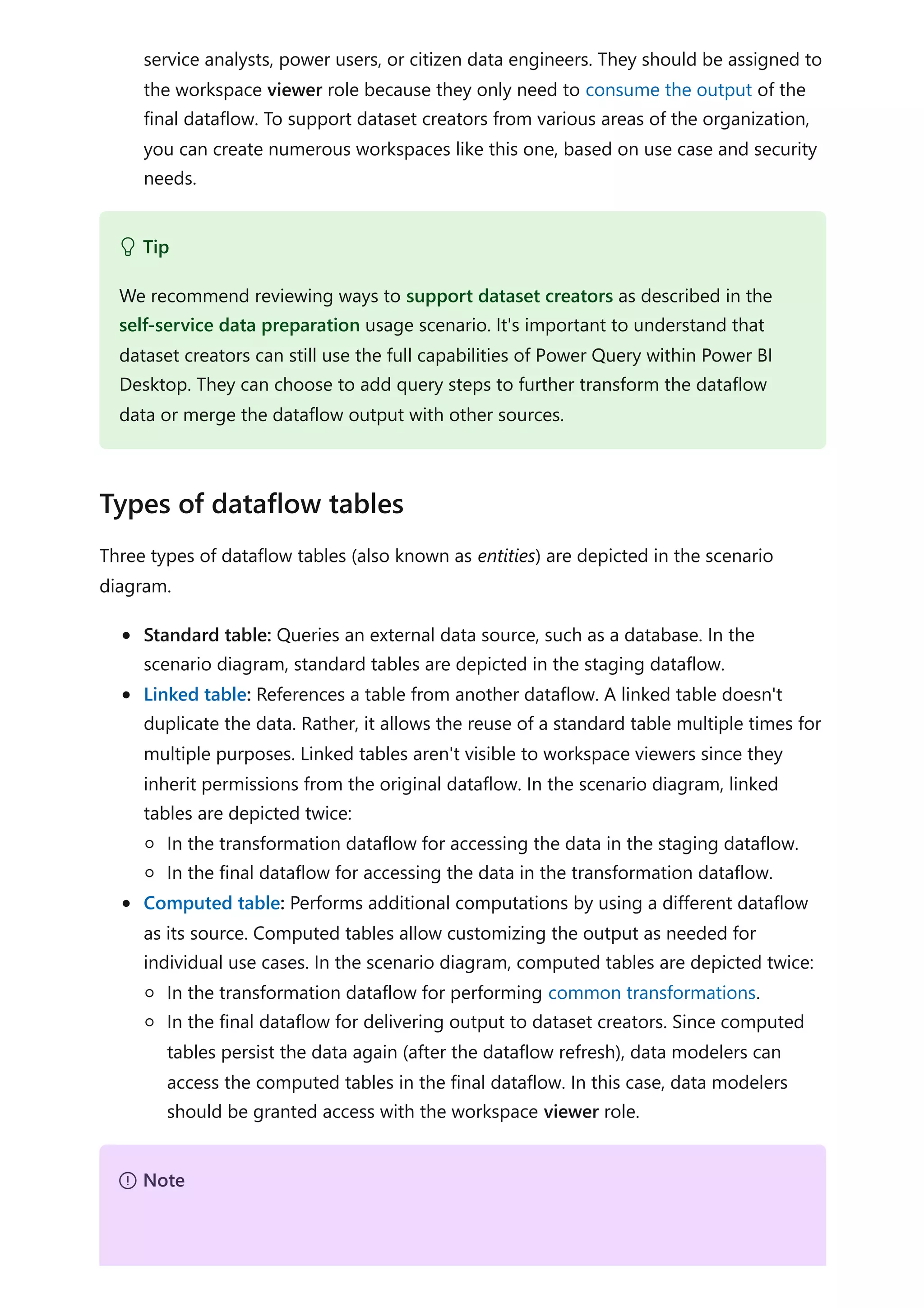
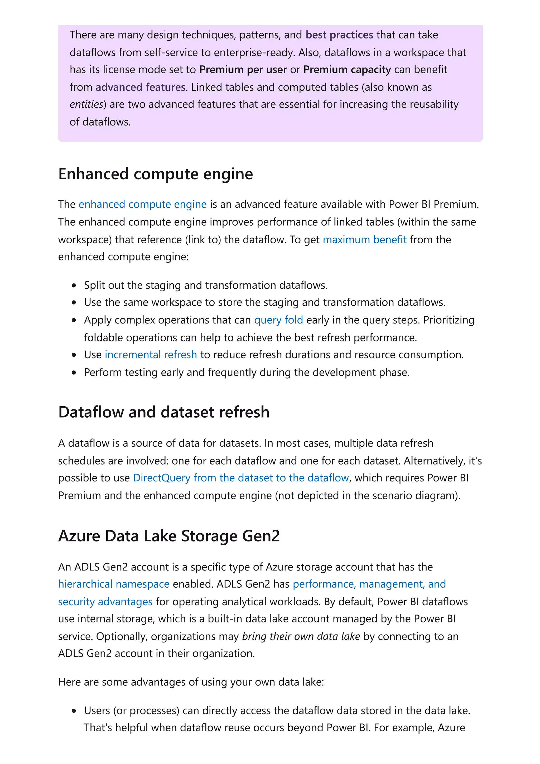

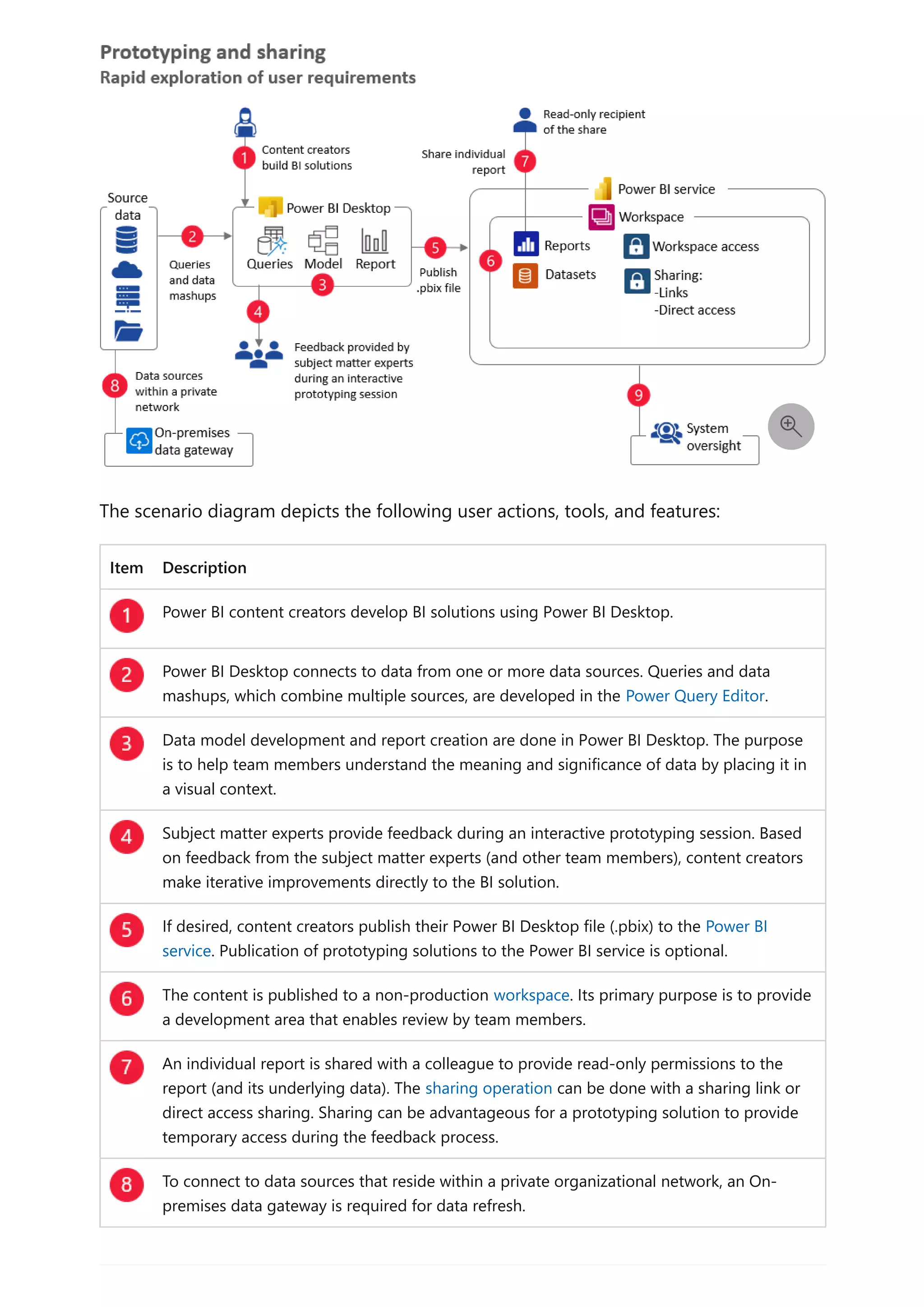


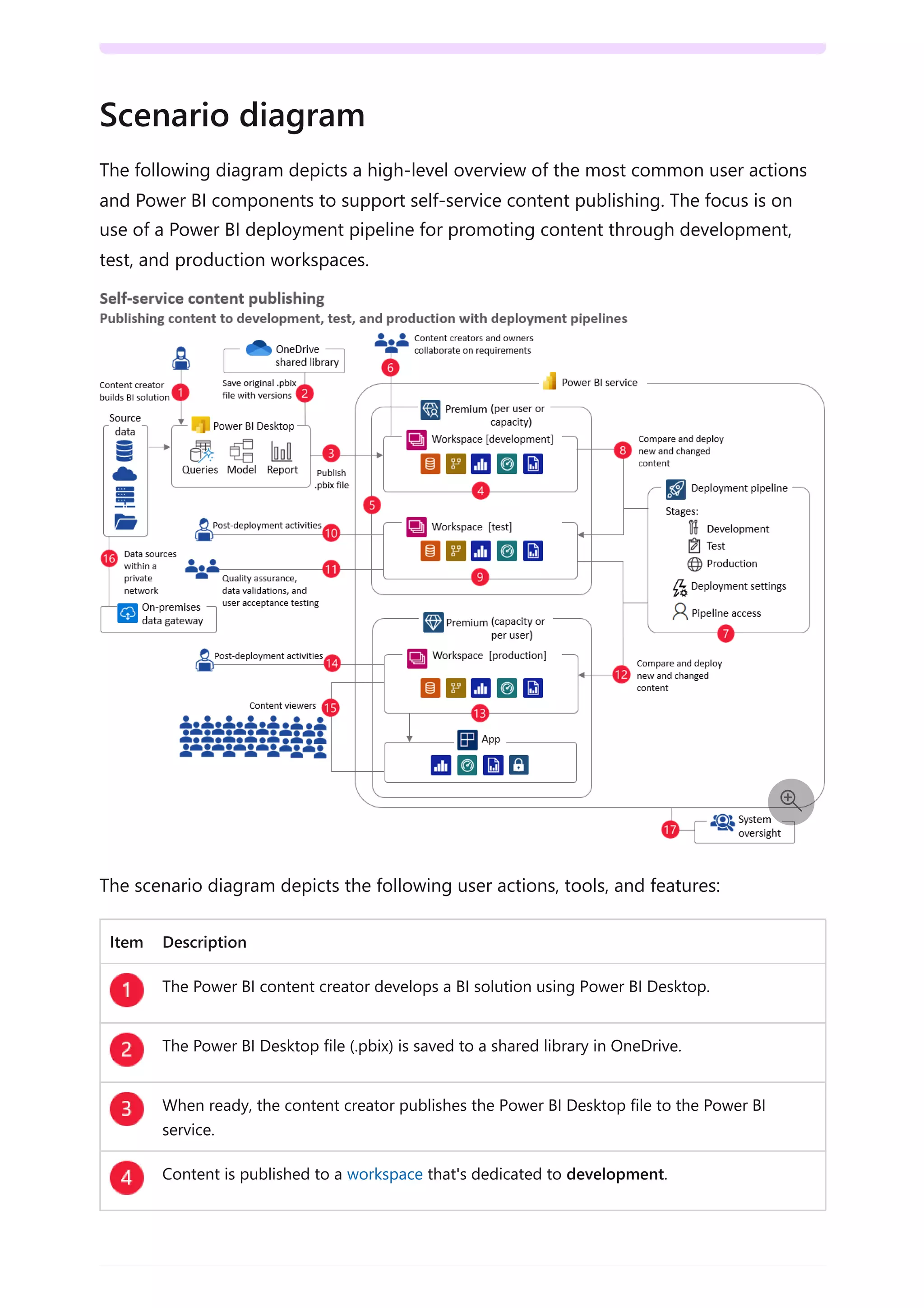
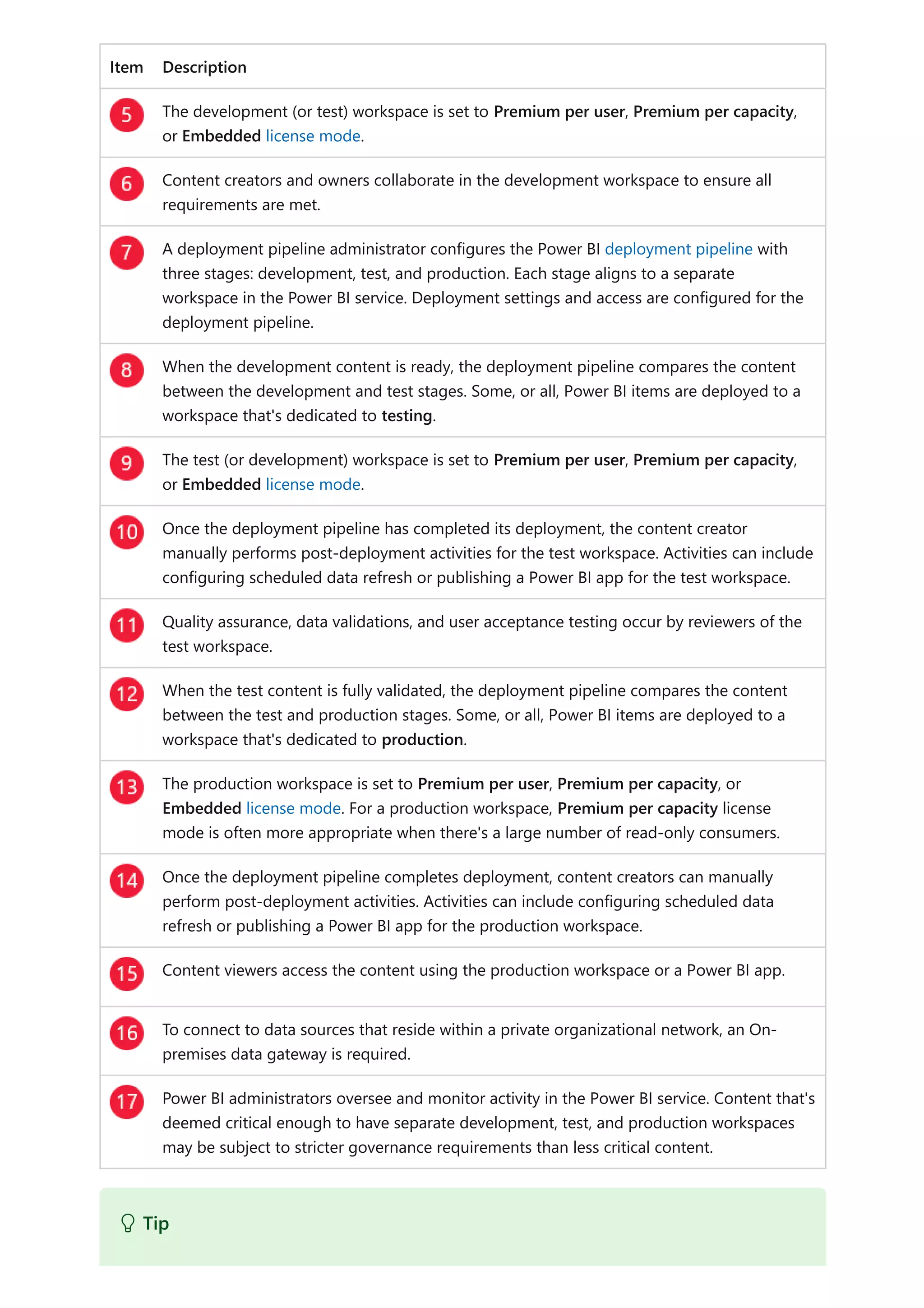
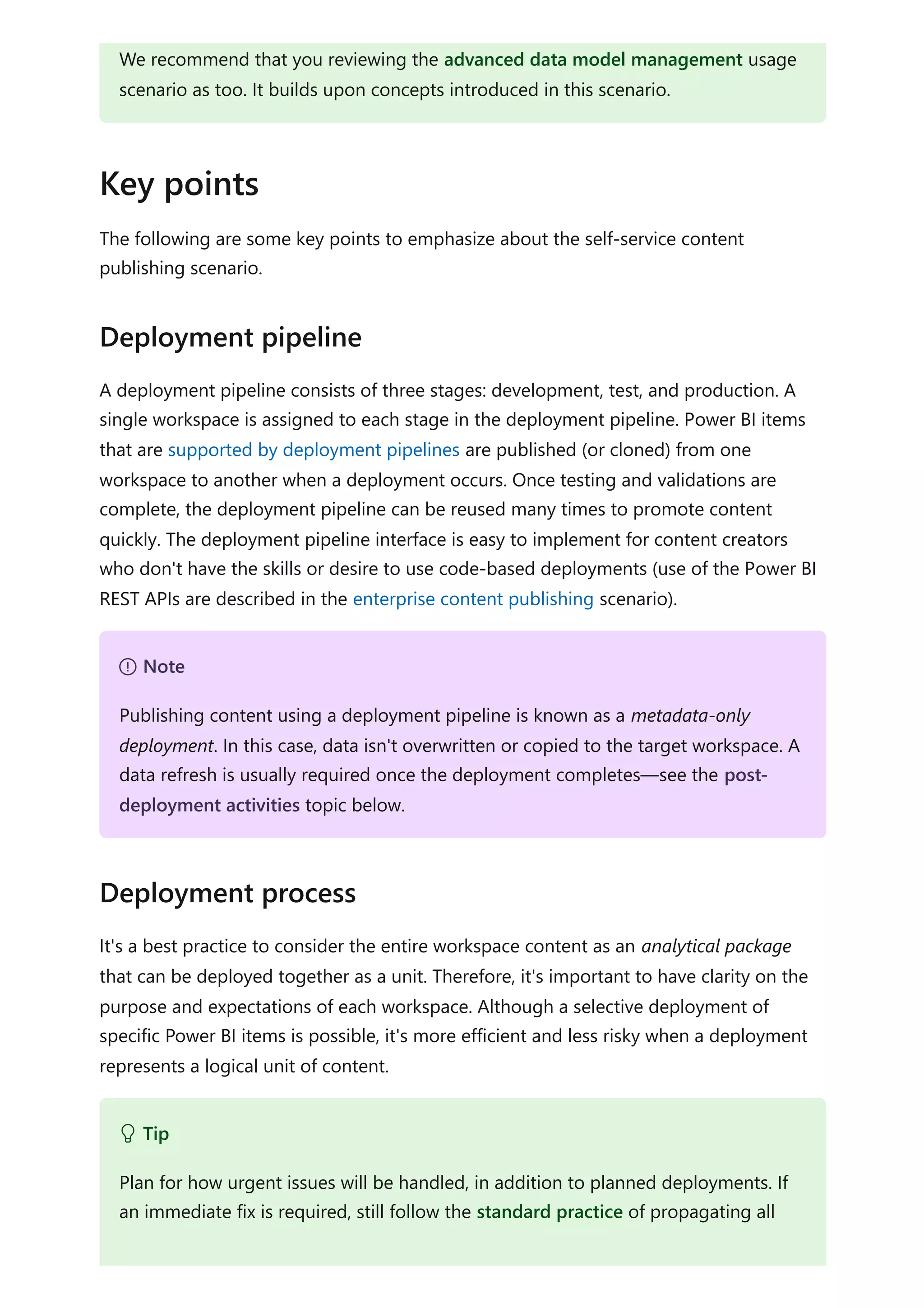


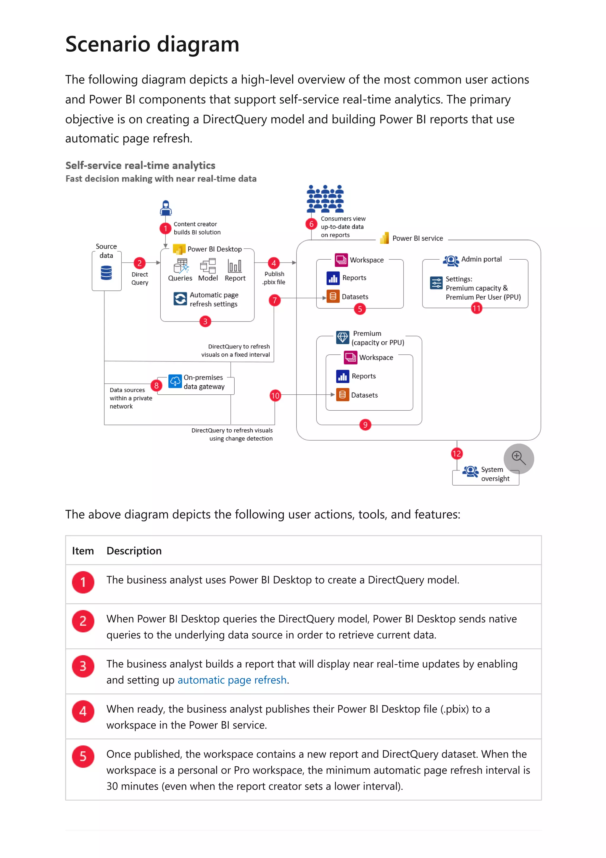
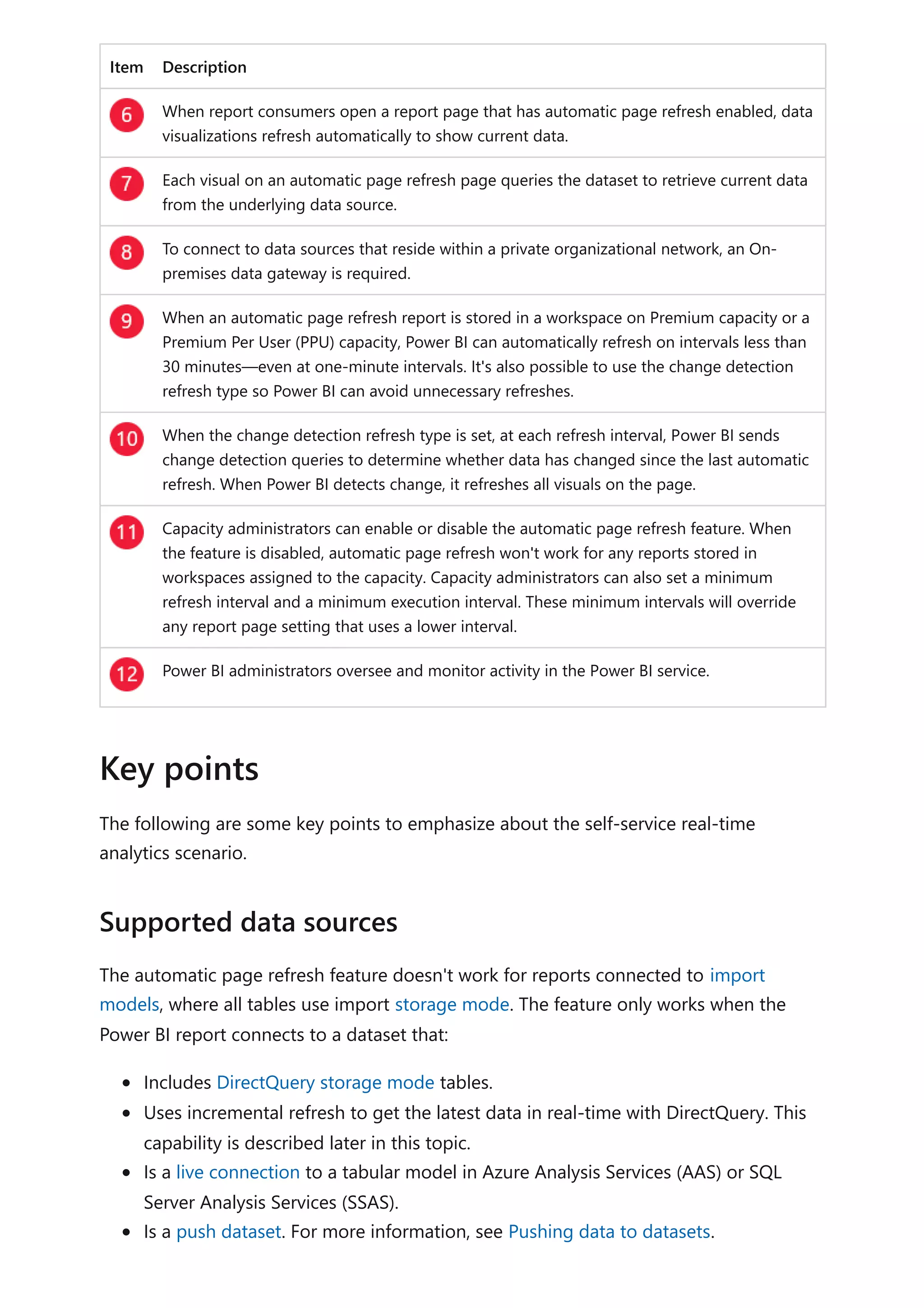
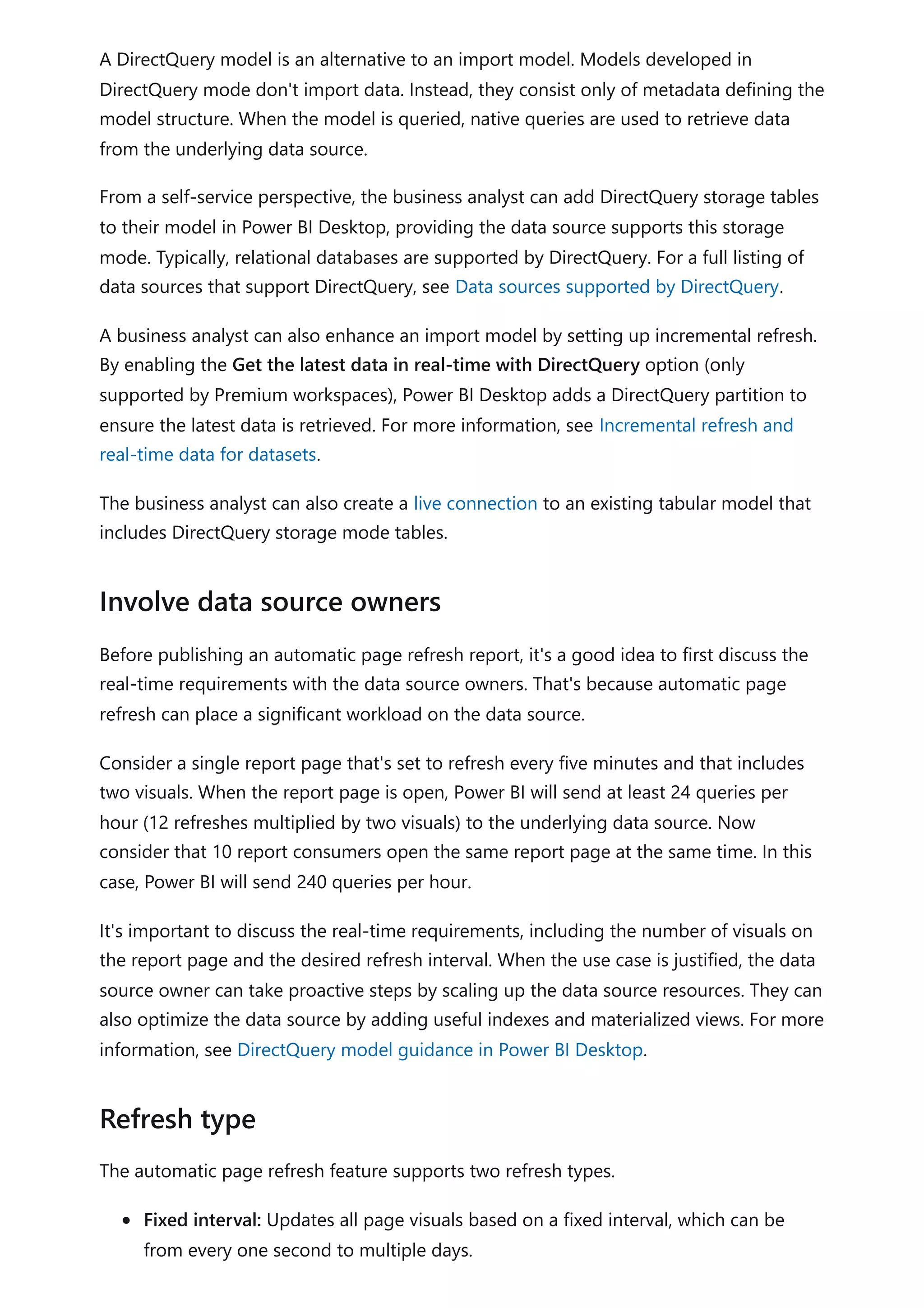
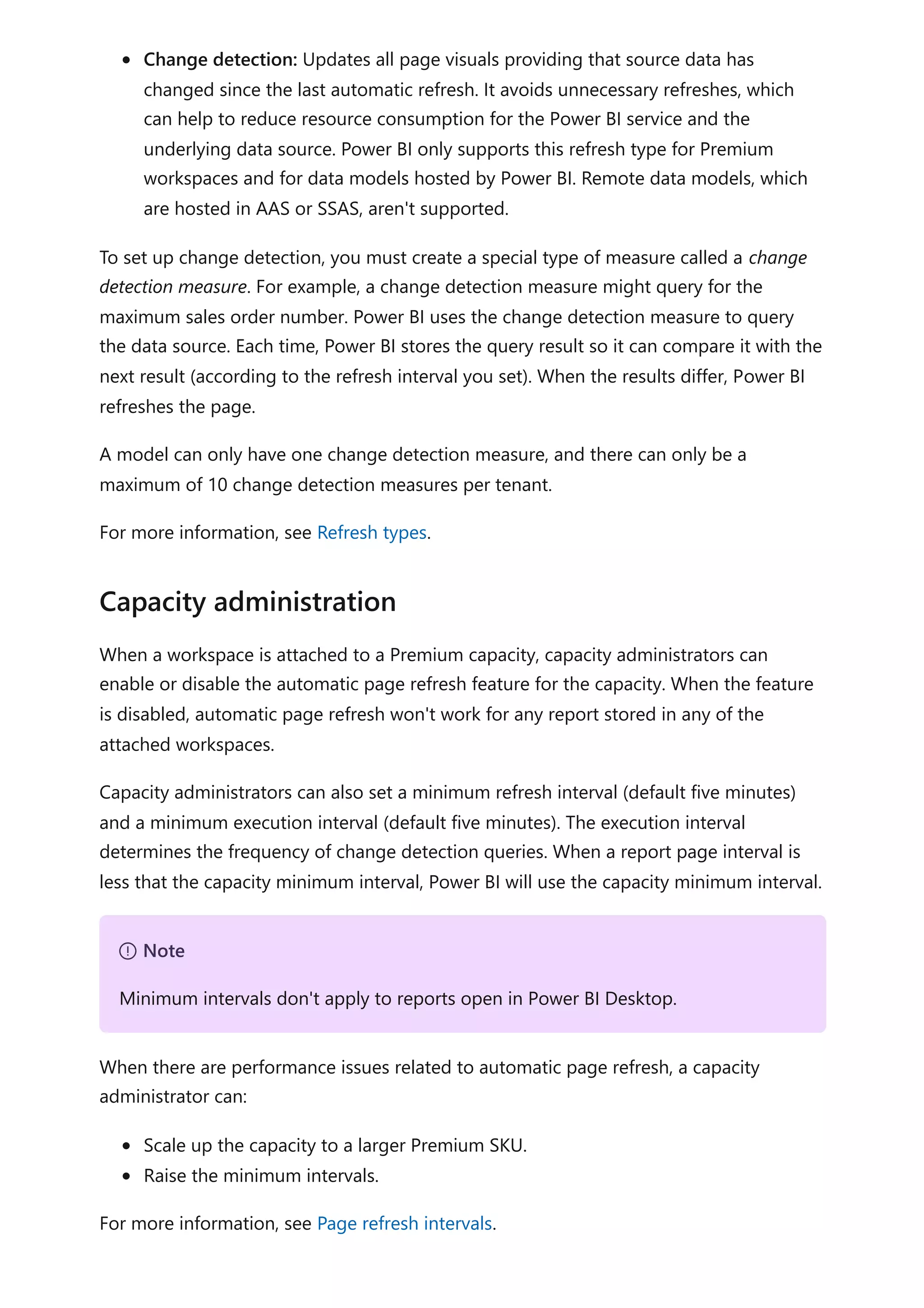
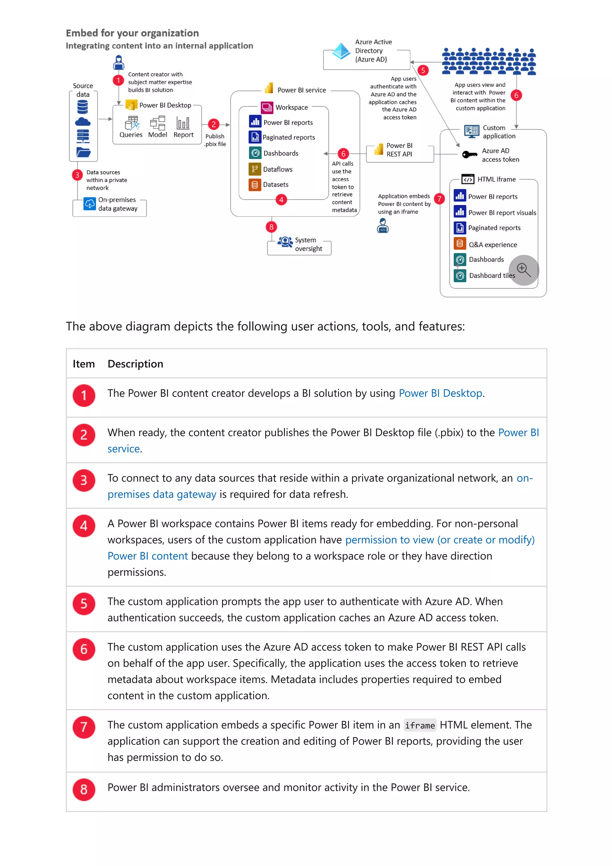

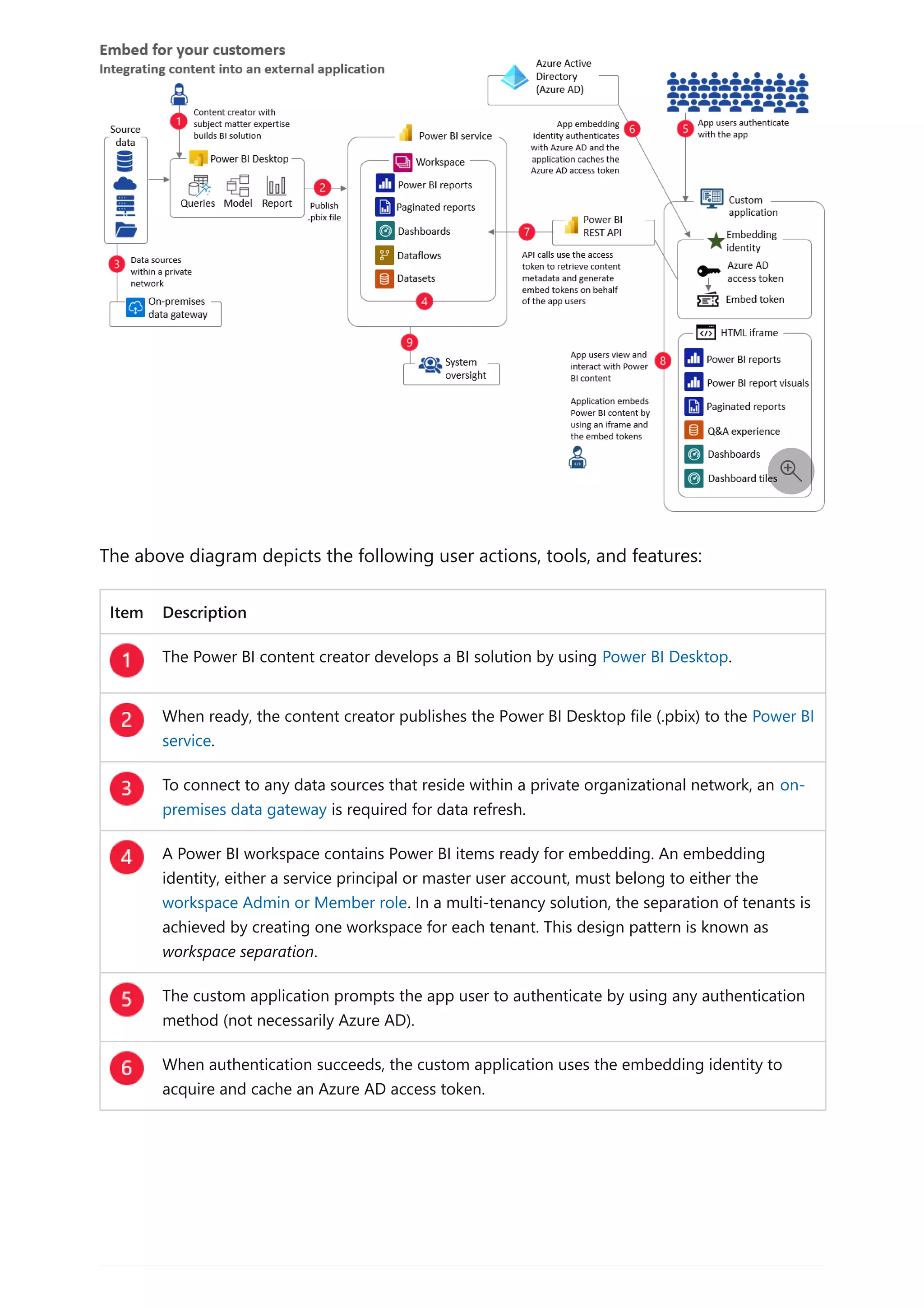
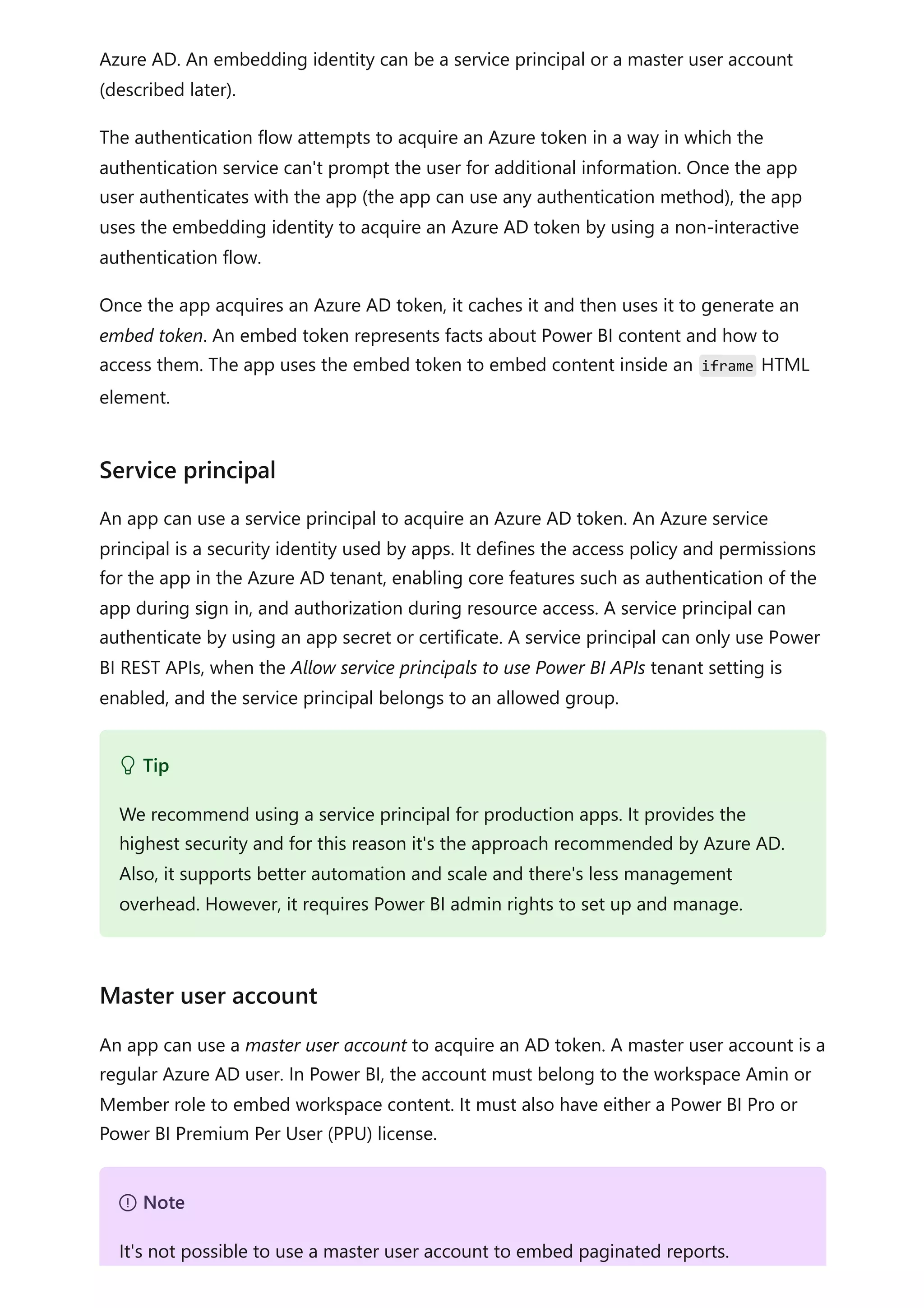
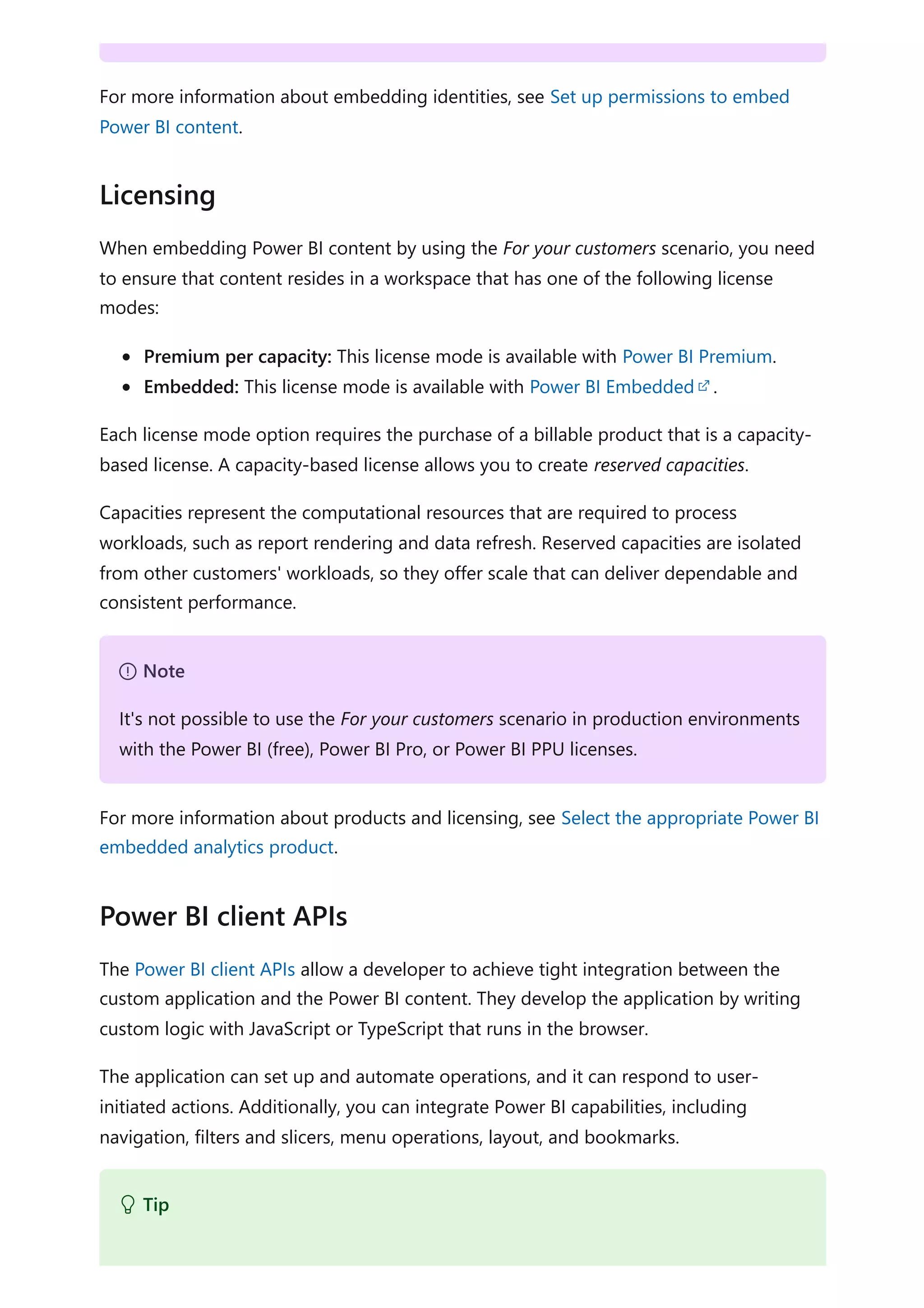
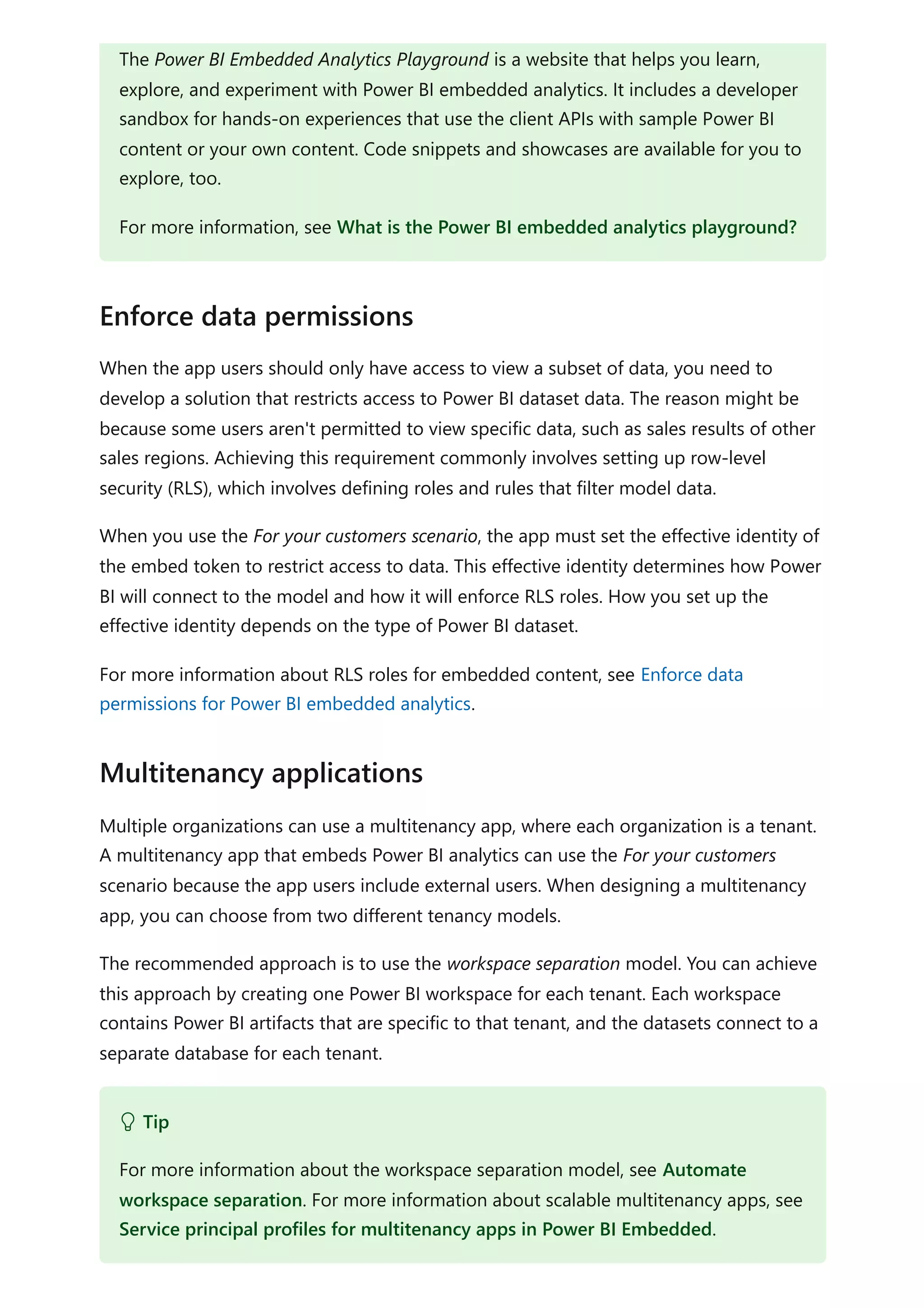

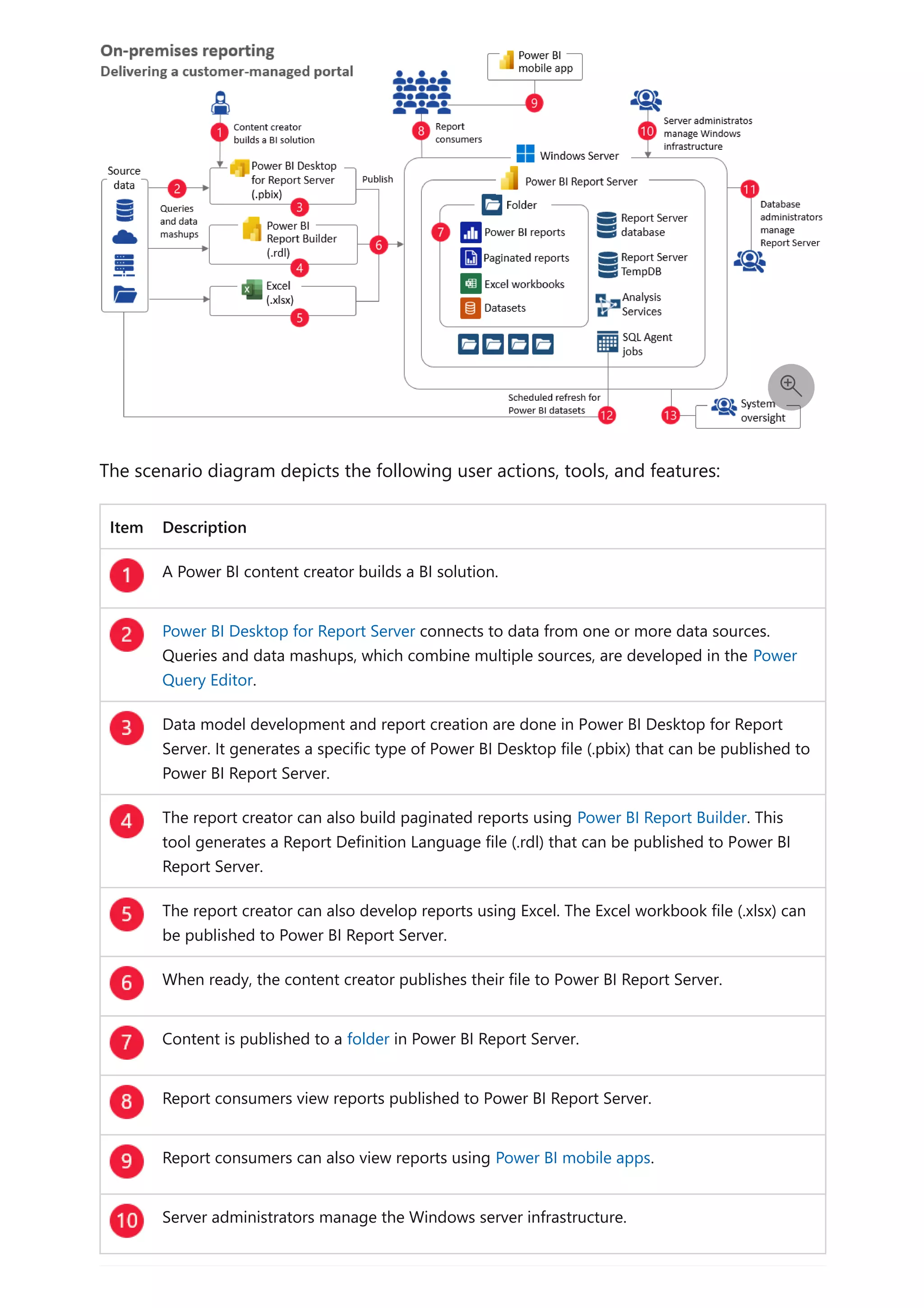

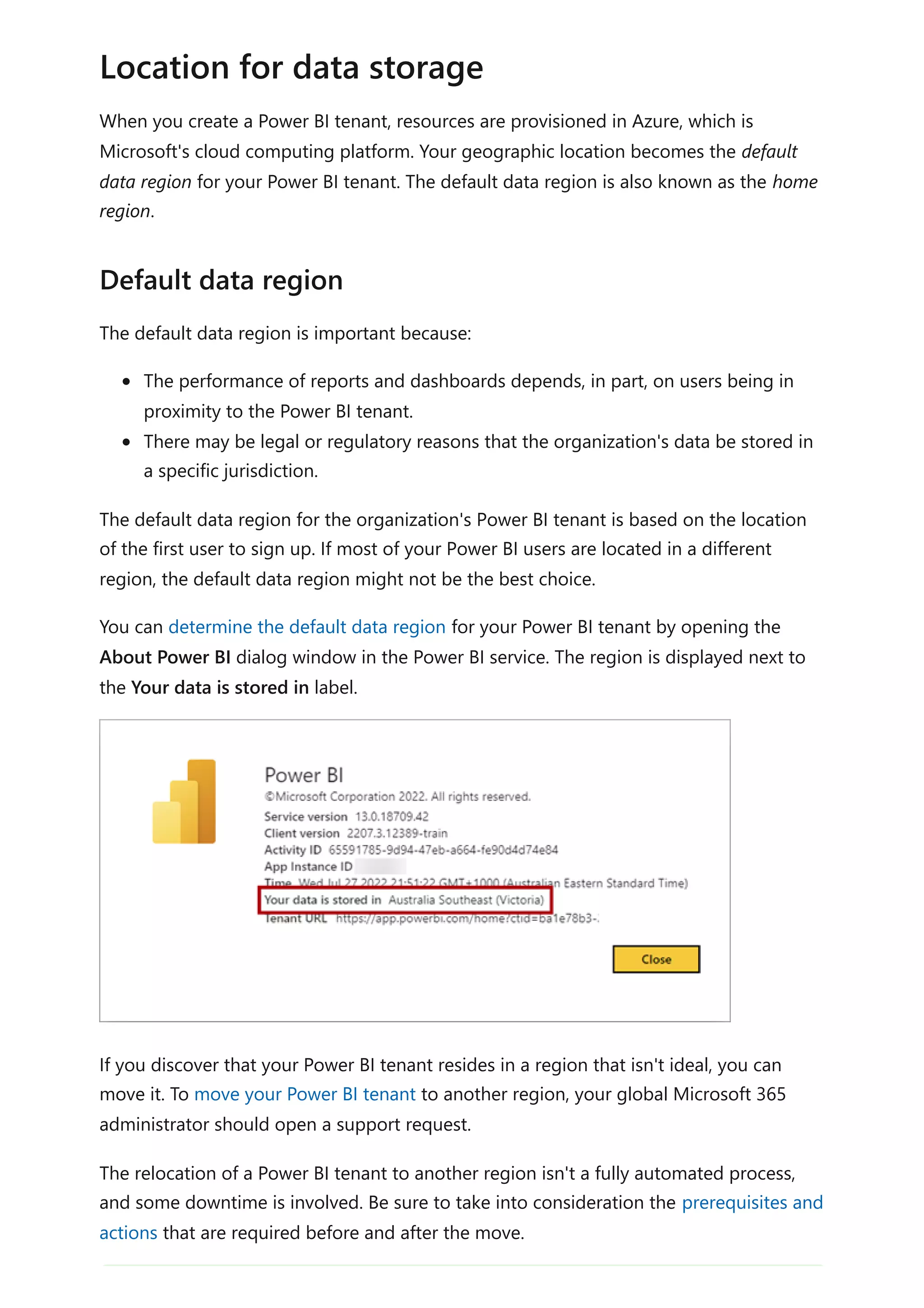


![recommend appending [Dev] or [Test] but leaving production as a user-friendly
name without a suffix. For example: FIN-Quarterly Financials [Dev].
Be consistent with the app name: The workspace name and its app can be
different, particularly if it improves usability or understandability for app
consumers. We recommend keeping the names at least similar to avoid confusion.
Omit unnecessary words: The following words may be redundant, so avoid them
in your workspace names:
The word workspace.
The words Power BI.
The name of the organization. However, when the primary audience is external
users, including the organization's name can be helpful.
Checklist - When considering creating workspace naming conventions, key decisions
and actions include:
7 Note
We recommend that you notify users when a workspace name will change. For the
most part, it's safe to rename a workspace in the Power BI service because the
GroupID, which is the unique identifier of a workspace, doesn't change (it's found in
the workspace URL). However, XMLA connections are impacted because they
connect by using the workspace name instead of the GroupID.
Determine requirements or preferences for workspace names: Consider how you
want to name your workspaces. Decide whether you want strict naming convention
requirements or more flexible requirements guided by suggestions and examples.
"
Review existing workspace names: Update existing workspace names as
appropriate so that they're good examples for users to follow. When users see
existing workspace being renamed, they'll interpret that as an implied standard to
adopt.
"
Create documentation for workspace naming conventions: Provide reference
documentation about workspace naming convention requirements and
preferences. Be sure to include examples that show the correct use of acronyms,
suffixes, and prefixes. Make the information available in your centralized portal and
training materials.
"](https://image.slidesharecdn.com/docpower-bi-guidance-230227102019-b6273799/75/DOC-Power-Bi-Guidance-pdf-604-2048.jpg)
![If you've decided to limit who can create workspaces, then the broader user population
will need to know what the process is to request a new workspace. In this case, it's
important to establish a request process that's easy and convenient for users to find and
follow.
It's also critical to respond quickly to a request for a new workspace. A service level
agreement (SLA) of 2-4 hours is ideal. If the process to request a new workspace is too
slow or burdensome, people will use the workspaces they have so they can keep
moving. If they elect to skip creating a new workspace, what they use instead may be
suboptimal. They might choose to reuse an existing workspace that isn't well-suited to
the new content, or they might share content from their personal workspace.
The following table lists the information to collect in a request for a new workspace.
Information
needed
Example Validation required
Workspace
name
SLS-Field Sales Analytics Does the name adhere to naming
conventions?
Does another workspace with the
same name exist?
Stages
needed
SLS-Field Sales Analytics [Dev], SLS-Field
Sales Analytics [Test], and SLS-Field Sales
Analytics
Are multiple workspaces necessary
to properly support the content?
If so, should a deployment pipeline
be created too?
Description Customer sales and order history for
monthly, quarterly, and yearly analysis.
Is there an expectation that
sensitive data, or regulated data,
will be stored?
If so, will that affect how the
workspace is governed?
Workspace creation process
Tip
The goal when creating a new process is to make it easy for people to comply with
the process. As with all data governance decisions, the point is to make it easy for
users to do the right thing.](https://image.slidesharecdn.com/docpower-bi-guidance-230227102019-b6273799/75/DOC-Power-Bi-Guidance-pdf-605-2048.jpg)


![Power BI reporting workspace members – Quarterly Financials
Power BI data workspace contributors – Quarterly Financials
Power BI reporting workspace contributors – Quarterly Financials
Power BI data workspace viewers – Quarterly Financials
Power BI reporting workspace viewers – Quarterly Financials
Power BI app viewers – Quarterly Financials
When multiple workspaces exist for development, test, and production, it results in an
even larger number of groups. There's the potential for the number of groups to triple.
For example, for just the data workspace admins, there would be these three groups:
Power BI data workspace admins – Quarterly Financials [Dev]
Power BI data workspace admins – Quarterly Financials [Test]
Power BI data workspace admins – Quarterly Financials
These examples are intended to convey that the use of groups that map to workspace
roles can quickly become unmanageable.
The effective use of groups for workspace roles can require considerable planning. Be
prepared to encounter scenarios when existing groups (that may be aligned with the
organizational chart) don't meet all your needs for managing Power BI content. In this
case, we recommend that you create groups specifically for this purpose. That's why the
words Power BI are included in the group name examples shown above. If you have
multiple business intelligence tools, you may choose to use only BI as the prefix rather
than Power BI. That way, you can use the same groups across multiple tools.
Lastly, the examples show one workspace - Quarterly Financials - but often it's possible
to manage a collection of workspaces with one set of groups. For example, multiple
workspaces owned and managed by the finance team could use the same groups.
Tip
There are times when fewer groups are needed, particularly in development. For
example, you may not need to specify a workspace viewers group in development;
that group may only be needed for test and production. Or you might be able to
use the same workspace admins group for development, test, and production.
7 Note
You'll often plan security more broadly, taking into consideration dataset Read and
Build permission requirements, and row-level security (RLS) requirements. For more
information about what to consider for security planning, see the security planning](https://image.slidesharecdn.com/docpower-bi-guidance-230227102019-b6273799/75/DOC-Power-Bi-Guidance-pdf-624-2048.jpg)


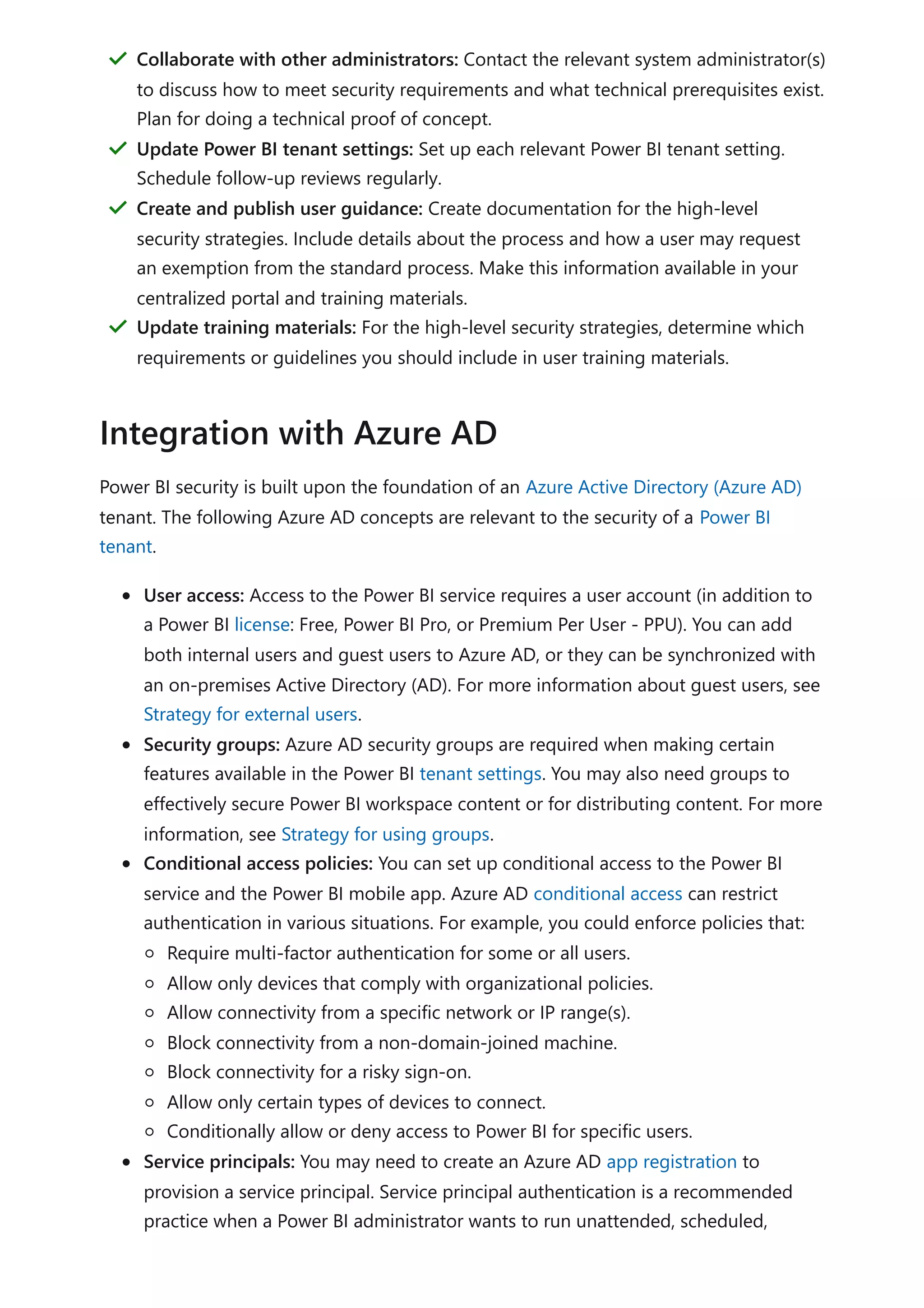
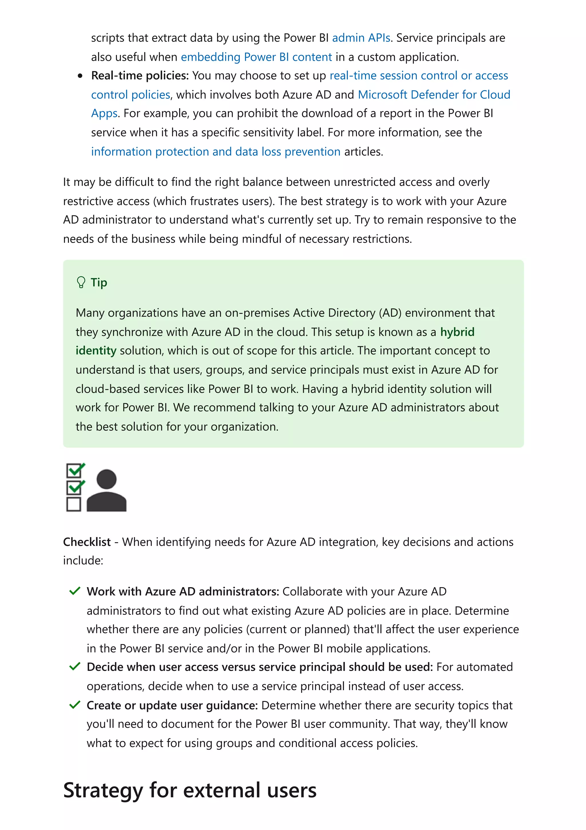
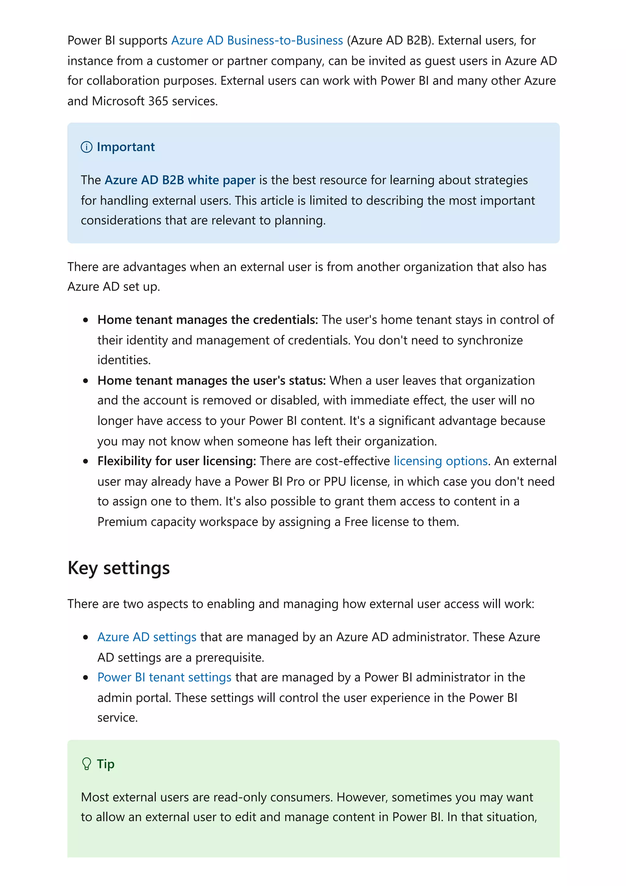
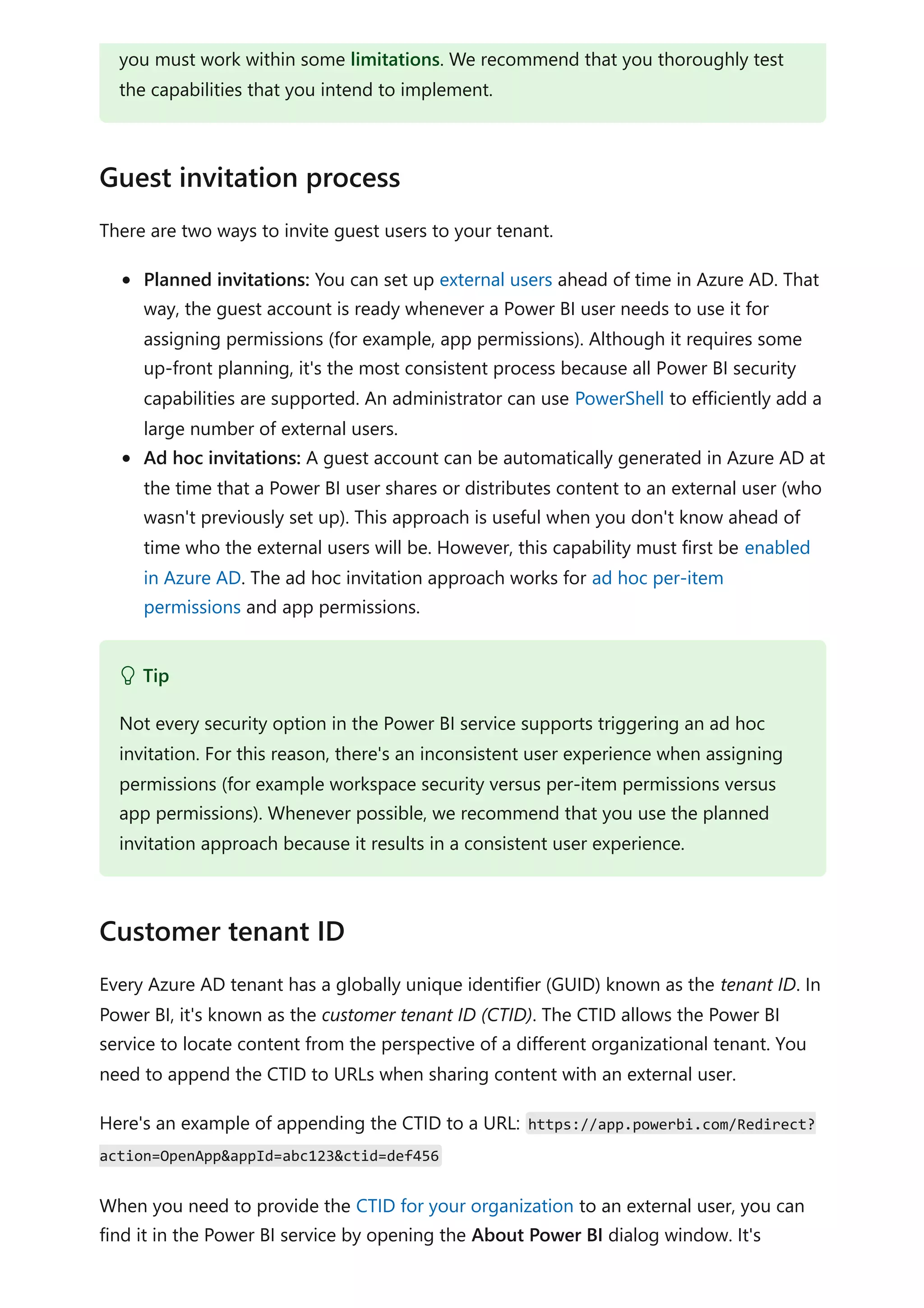
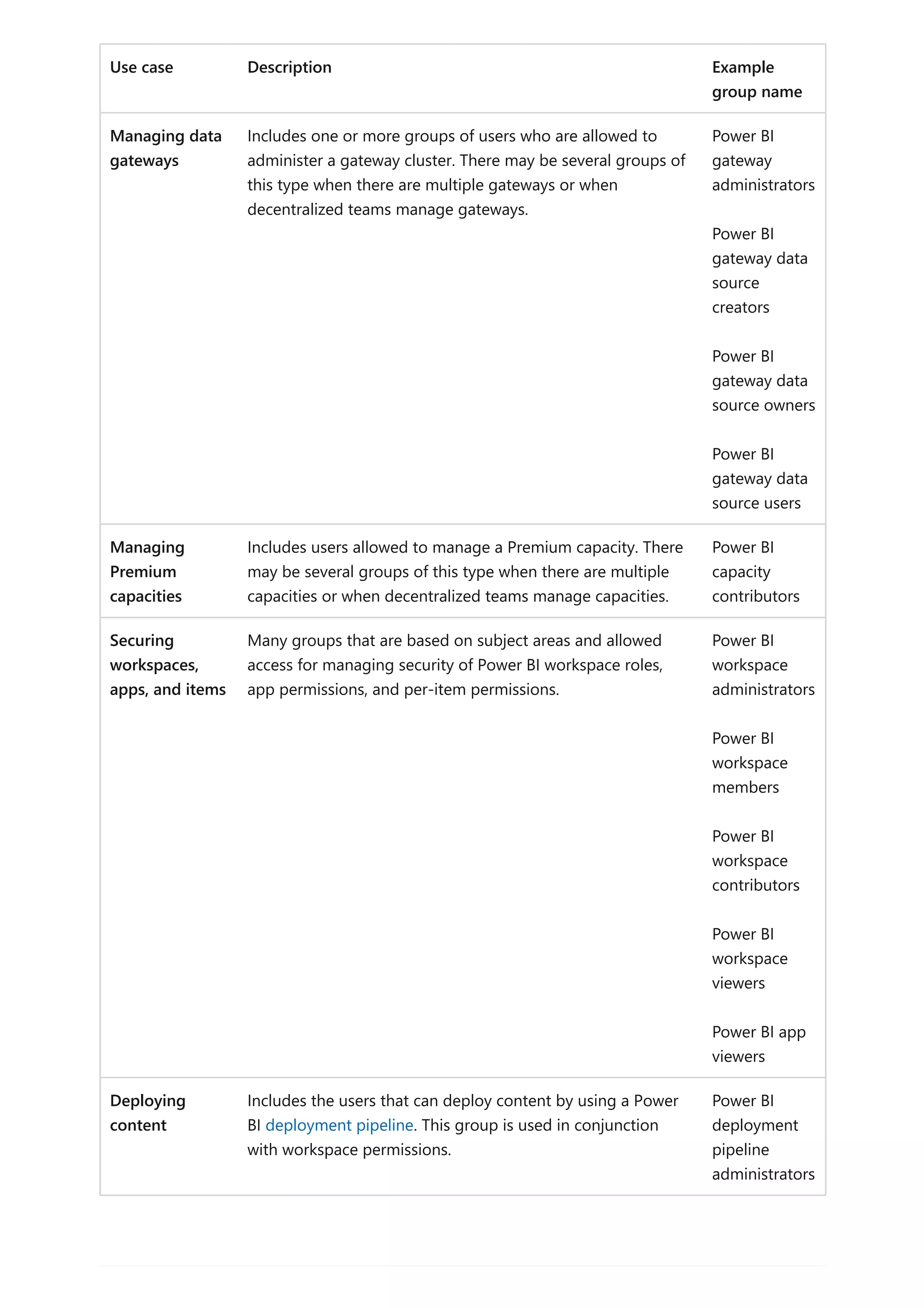
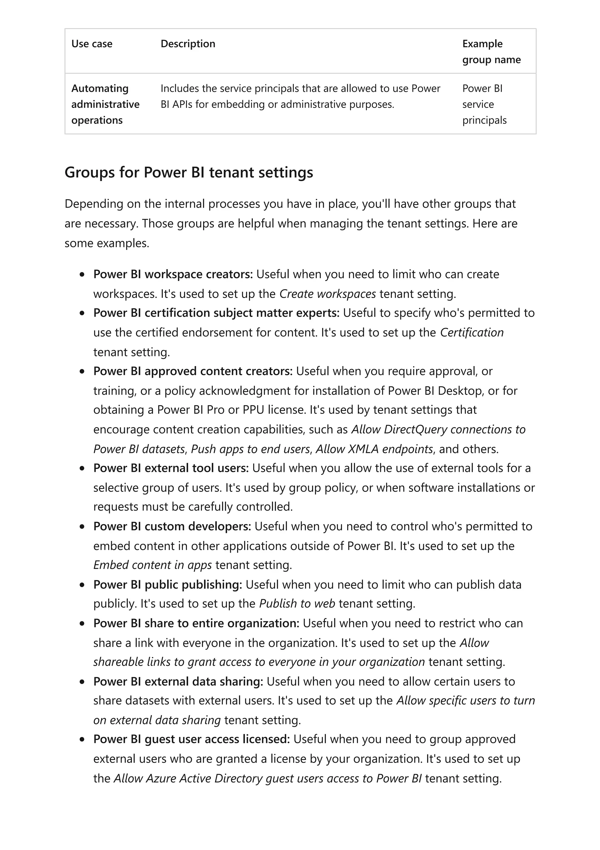
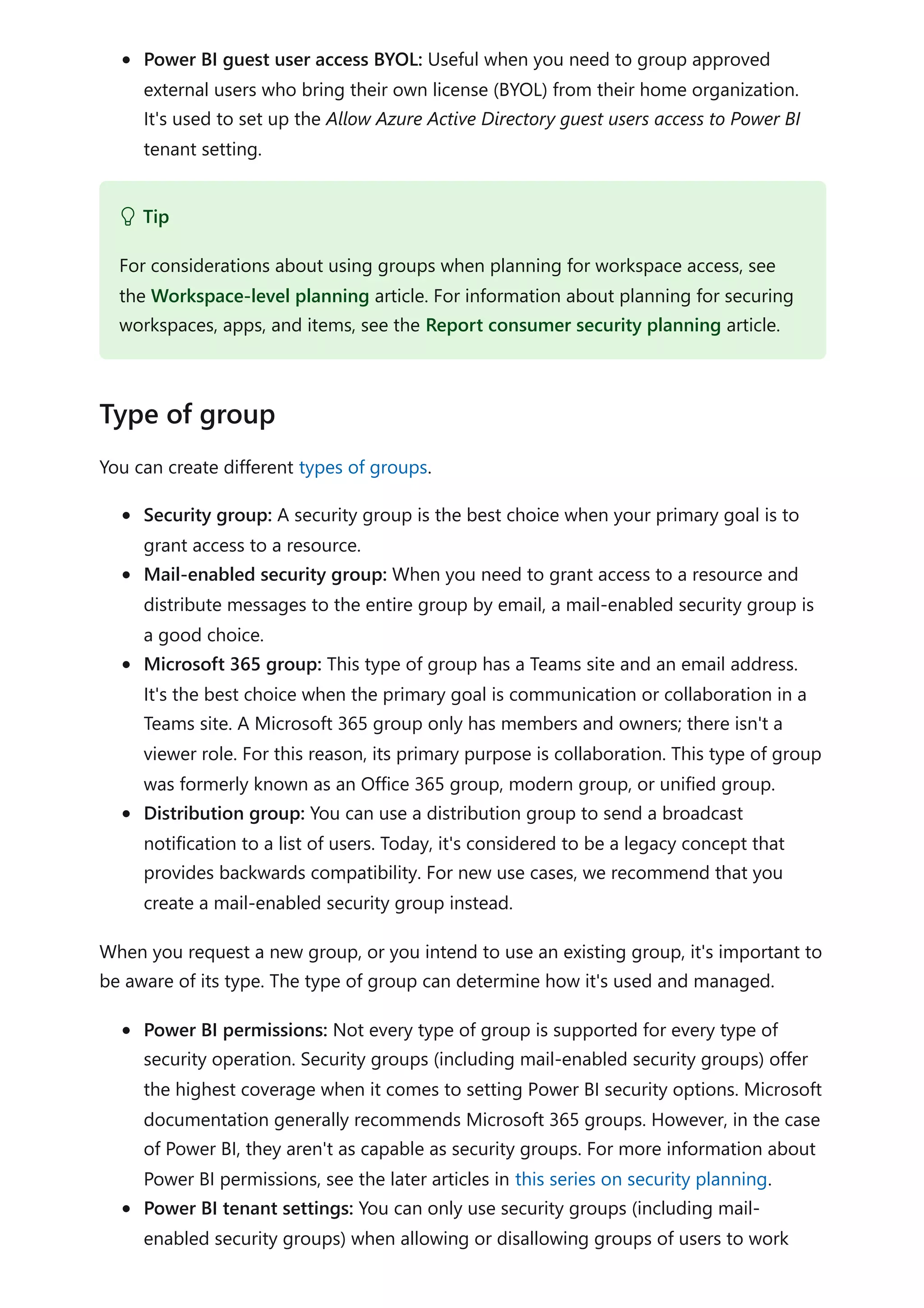
![with Power BI tenant settings.
Advanced Azure AD features: Certain types of advanced features aren't supported
for all group types. For example, you might want to manage group membership
dynamically based on an attribute in Azure AD (such as the department for a user,
or even a custom attribute). Only Microsoft 365 groups and security groups
support dynamic group memberships. Or, if you want to nest a group within a
group, be aware that Microsoft 365 groups don't support that capability.
Managed differently: Your request to create or manage a group might be routed
to a different administrator based on the type of group (mail-enabled security
groups and distribution groups are managed in Exchange). Therefore, your internal
process will differ depending on the type of group.
It's likely that you'll end up with many groups in Azure AD to support your Power BI
implementation. Therefore, it's important to have an agreed-upon pattern for how
groups are named. A good naming convention will help to determine the purpose of
the group and make it simpler to manage.
Consider using the following standard naming convention: <Prefix> <Purpose> -
<Topic/Scope/Department> <[Environment]>
The following list describes each part of the naming convention.
Prefix: Used to group all Power BI groups together. When the group will be used
for more than one analytical tool, your prefix might be just BI, rather than Power BI.
In that case, the text that describes the purpose will be more generic so that it
relates to more than one analytical tool.
Purpose: The purpose will vary. It could be for a workspace role, app permissions,
item-level permissions, row-level security, or other purpose. Sometimes multiple
purposes can be satisfied with a single group.
Topic/Scope/Department: Used to clarify who the group applies to. It will often
describe the group membership. It can also refer to who manages the group.
Sometimes a single group can be used for multiple purposes. For example, a
collection of finance workspaces could be managed with a single group.
Environment: Optional. Useful to differentiate between development, test, and
production.
Here are some example group names that apply the standard naming convention.
Power BI workspace admins - Finance [Dev]
Power BI workspace members - Finance [Dev]
Group naming convention](https://image.slidesharecdn.com/docpower-bi-guidance-230227102019-b6273799/75/DOC-Power-Bi-Guidance-pdf-653-2048.jpg)
![Power BI workspace contributors - Finance [Dev]
Power BI workspace viewers - Finance [Dev]
Power BI app viewers - Finance
Power BI gateway administrators - Enterprise BI
Power BI gateway administrators - Finance
When planning for which groups you'll need, several decisions must be made.
When a content creator or owner requests a new group, ideally they use a form to
provide the following information.
Name and purpose: A suggested group name and its intended purpose. Consider
including Power BI (or just BI when you have multiple BI tools) in the group name
to clearly indicate the scope of the group.
Email address: An email address when communication is also required for the
group members. Not all types of groups need to be mail-enabled.
Type of group: Options include security group, mail-enabled security group,
Microsoft 365 group, and distribution group.
Group owner: Who's allowed to own and manage the members of the group.
Group membership: The intended users who will be members of the group.
Consider whether external users and internal users can be added, or whether
there's a justification for putting external users into a different group.
Use of just-in-time group member assignment: You can use Privileged Identity
Management (PIM) to allow time-boxed, just-in-time, access to a group. This
service can be helpful when users require temporary access. PIM is also helpful for
Power BI administrators who need occasional access.
Checklist - When creating your strategy for how to use groups, key decisions and
actions include:
Decisions per group
Tip
Existing groups that are based on the organizational chart don't always work well
for Power BI purposes. Use existing groups when they meet your needs. However,
be prepared to create Power BI-specific groups when the need arises.](https://image.slidesharecdn.com/docpower-bi-guidance-230227102019-b6273799/75/DOC-Power-Bi-Guidance-pdf-654-2048.jpg)
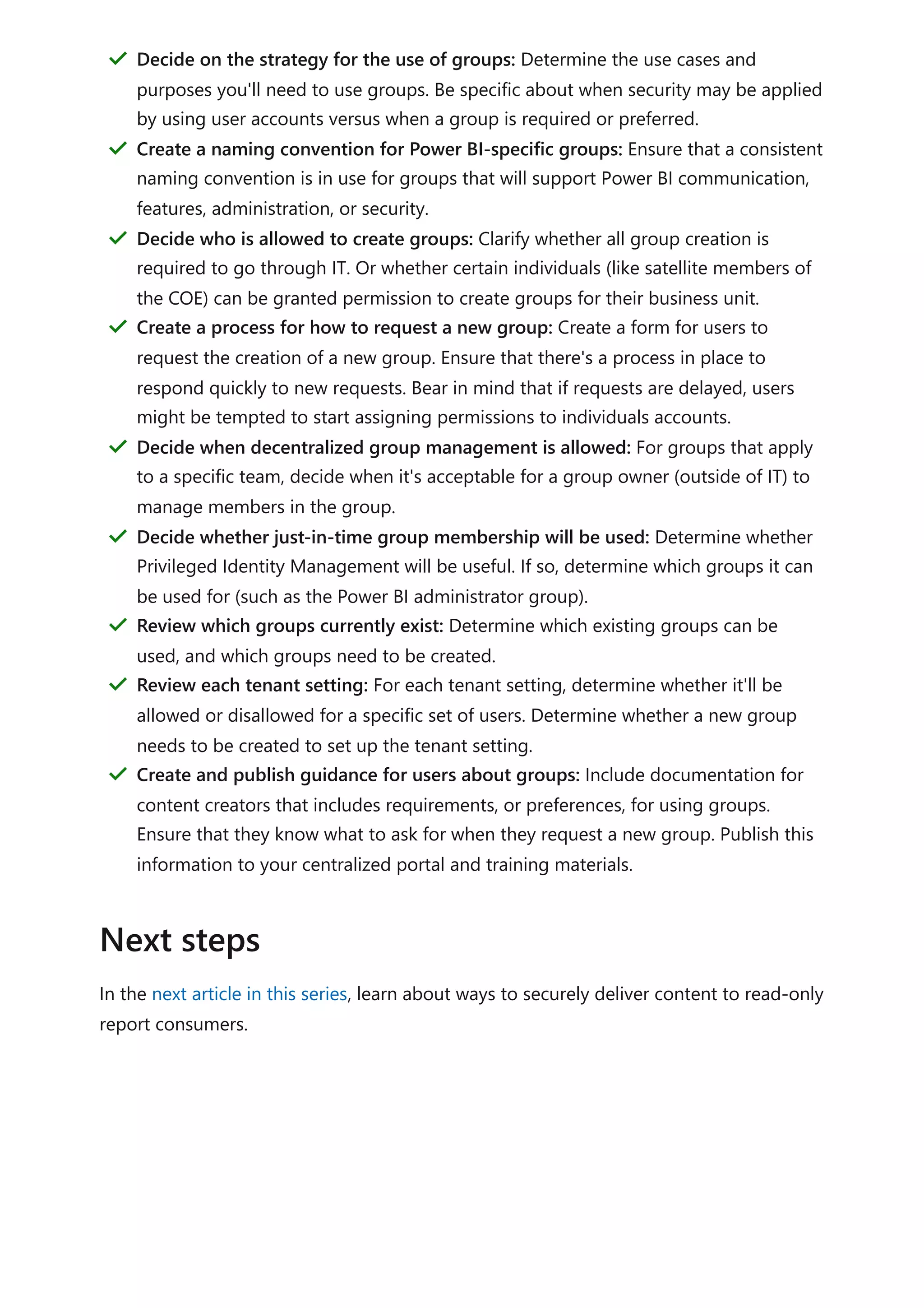

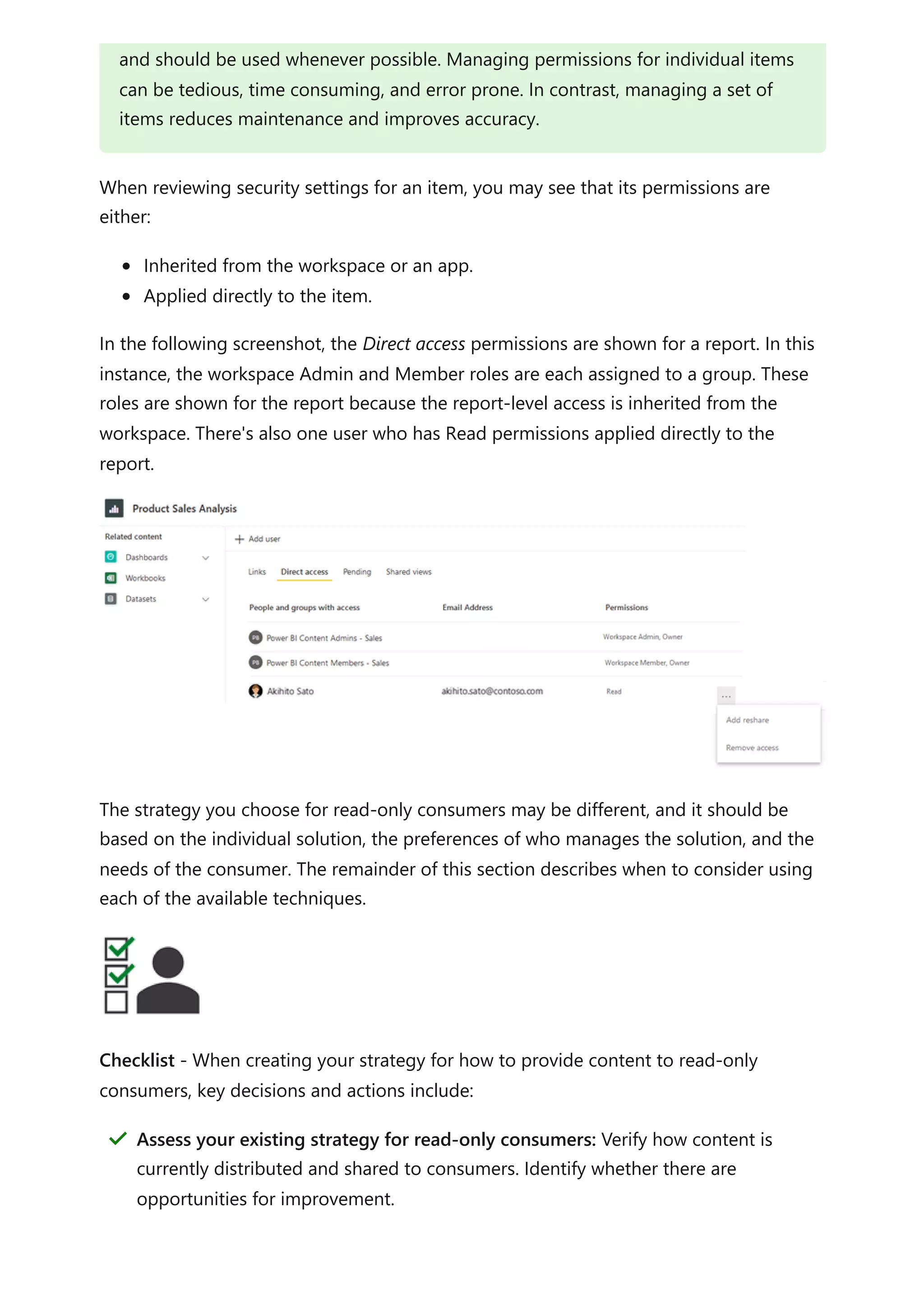
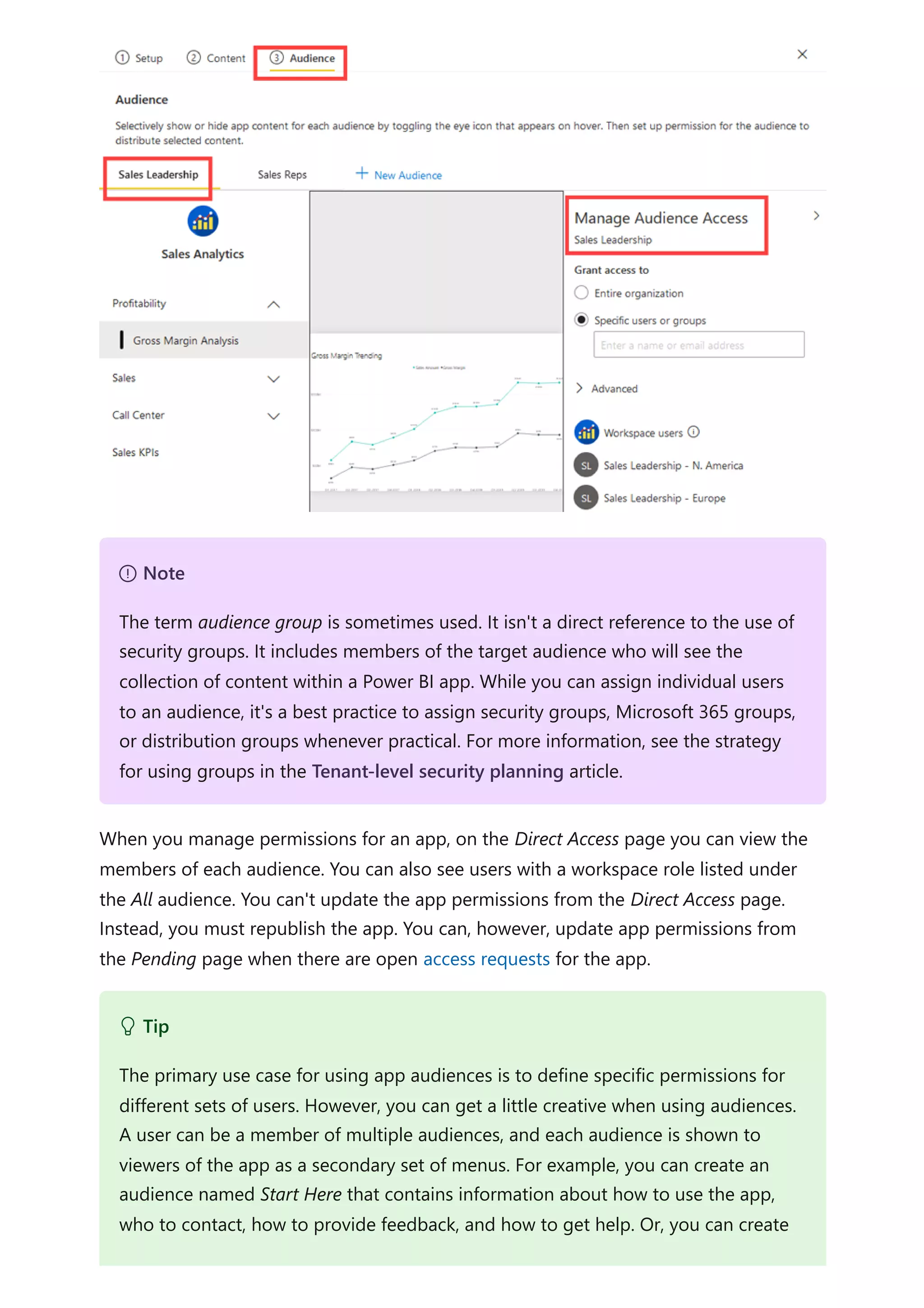
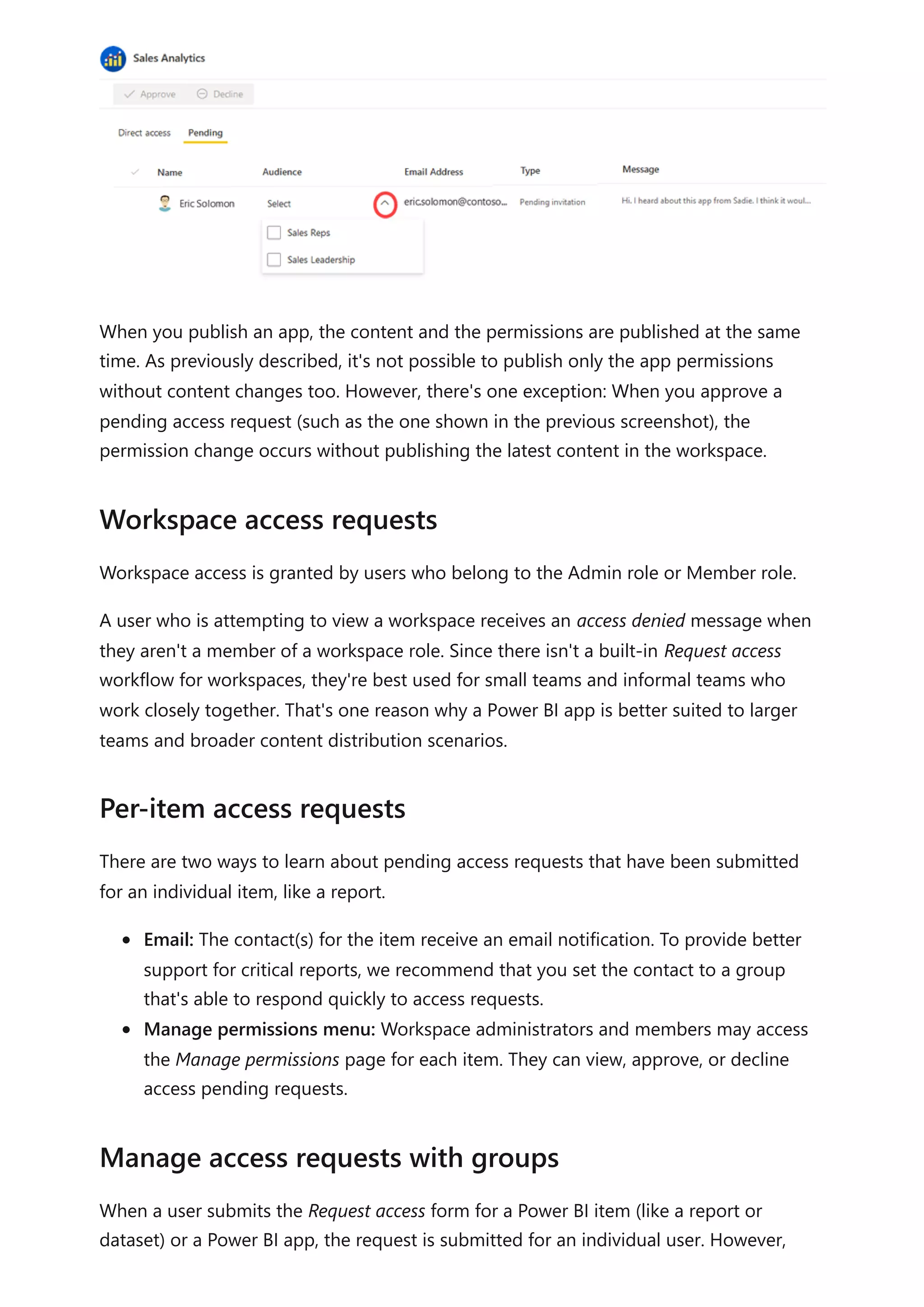
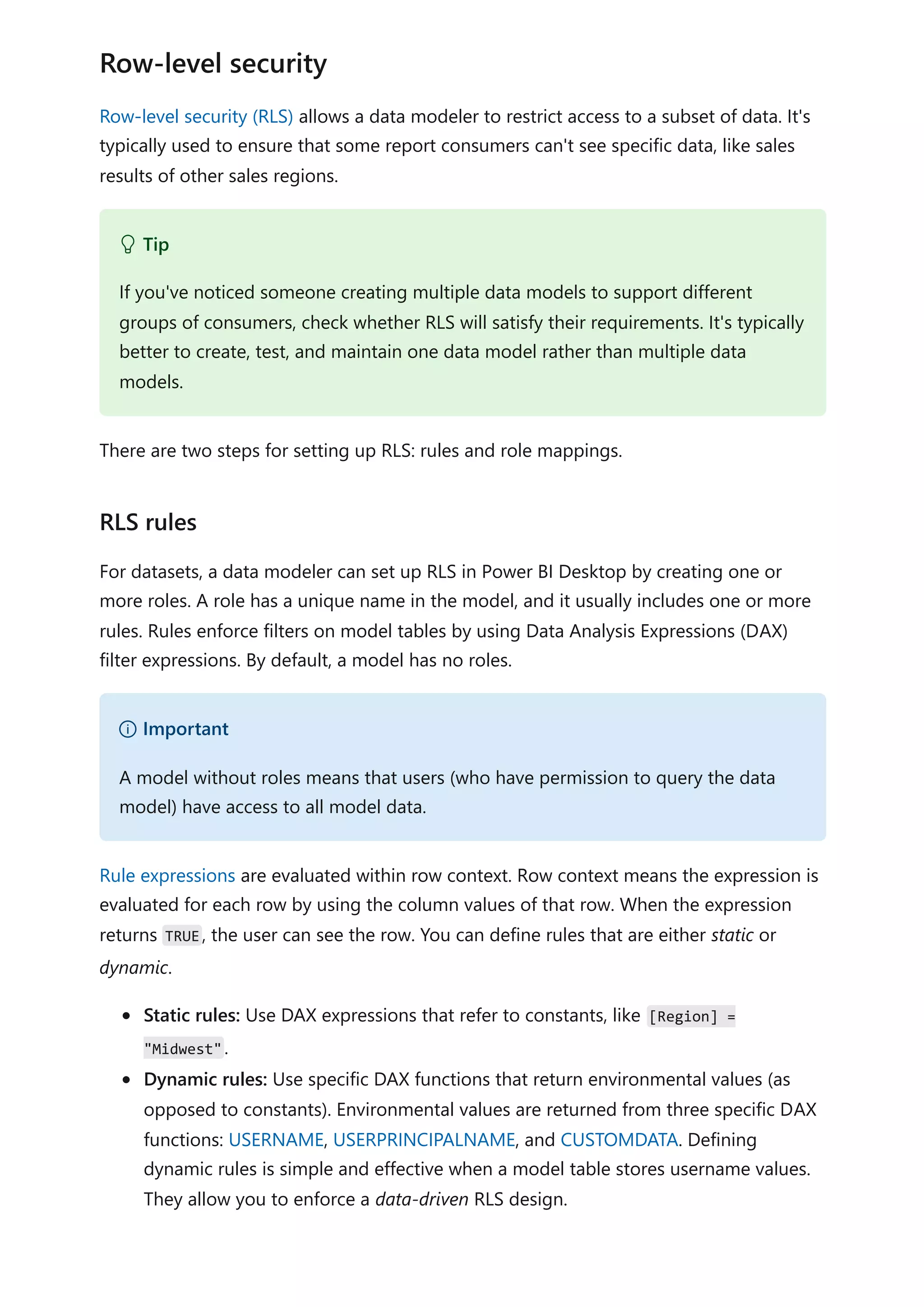
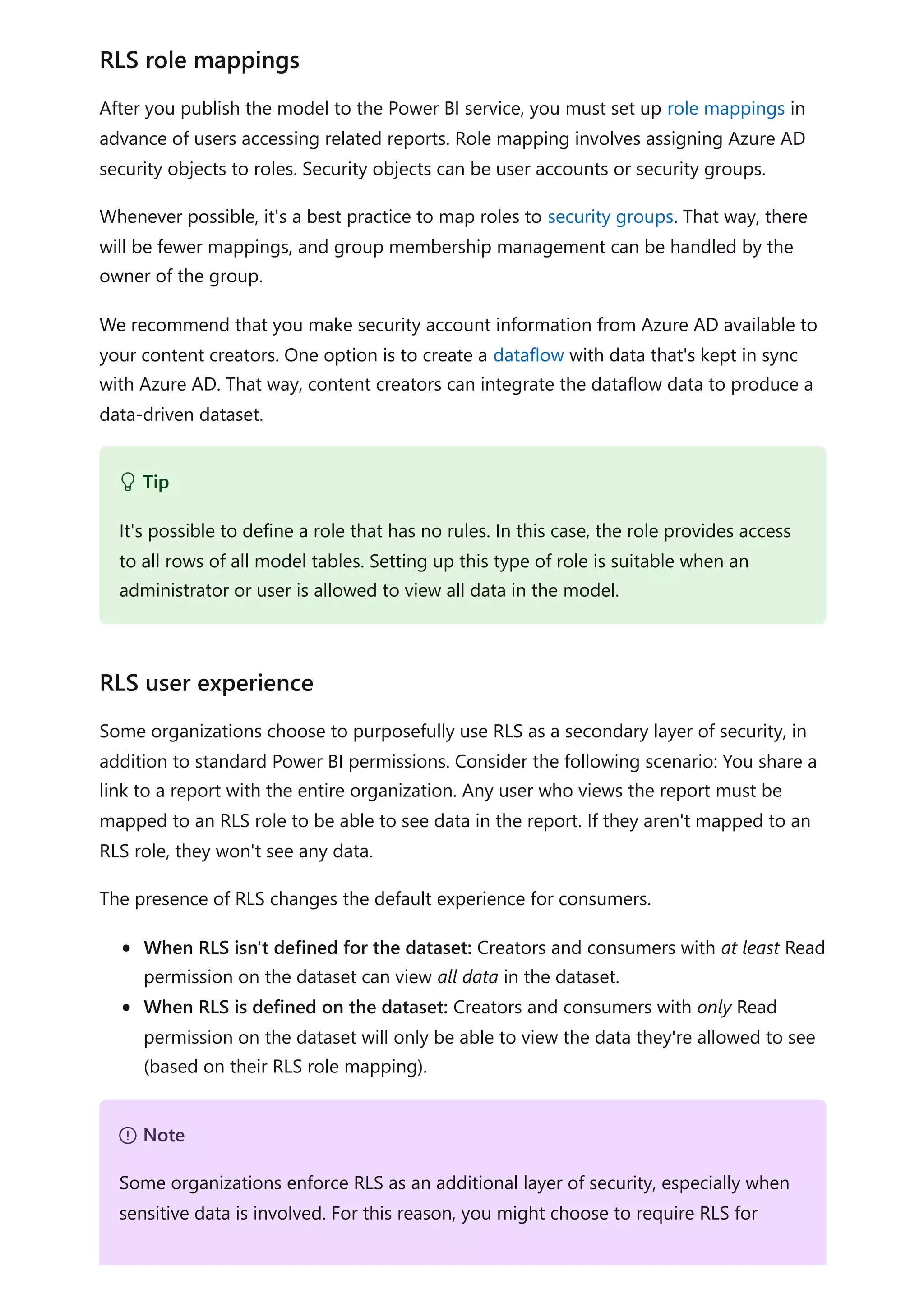
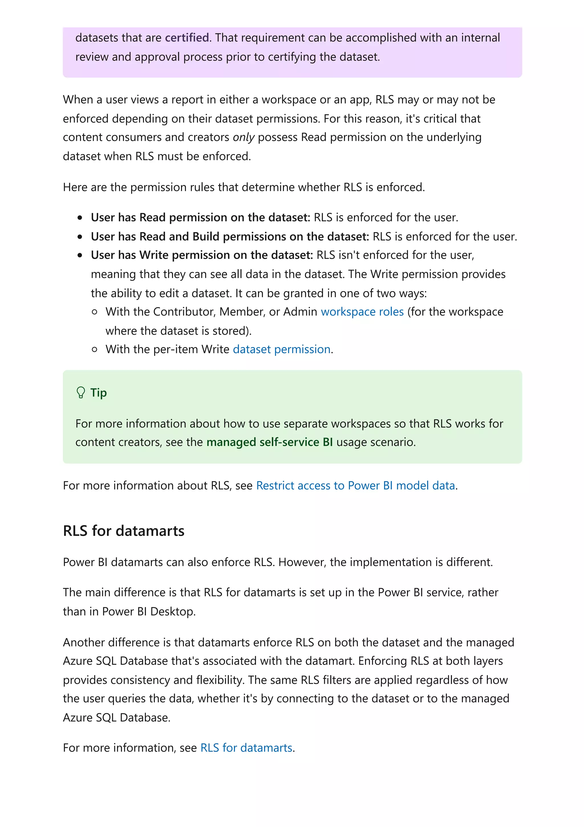
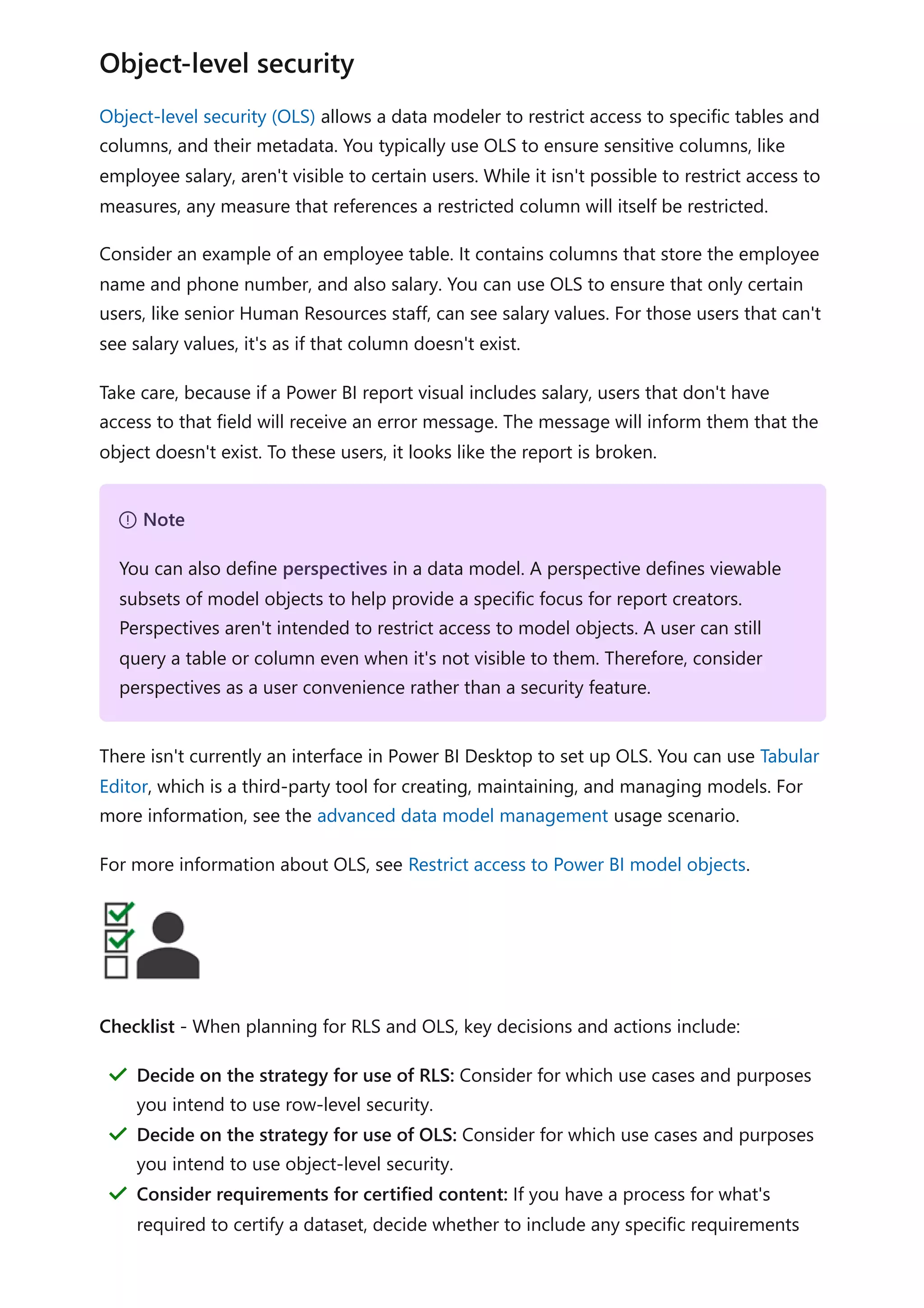
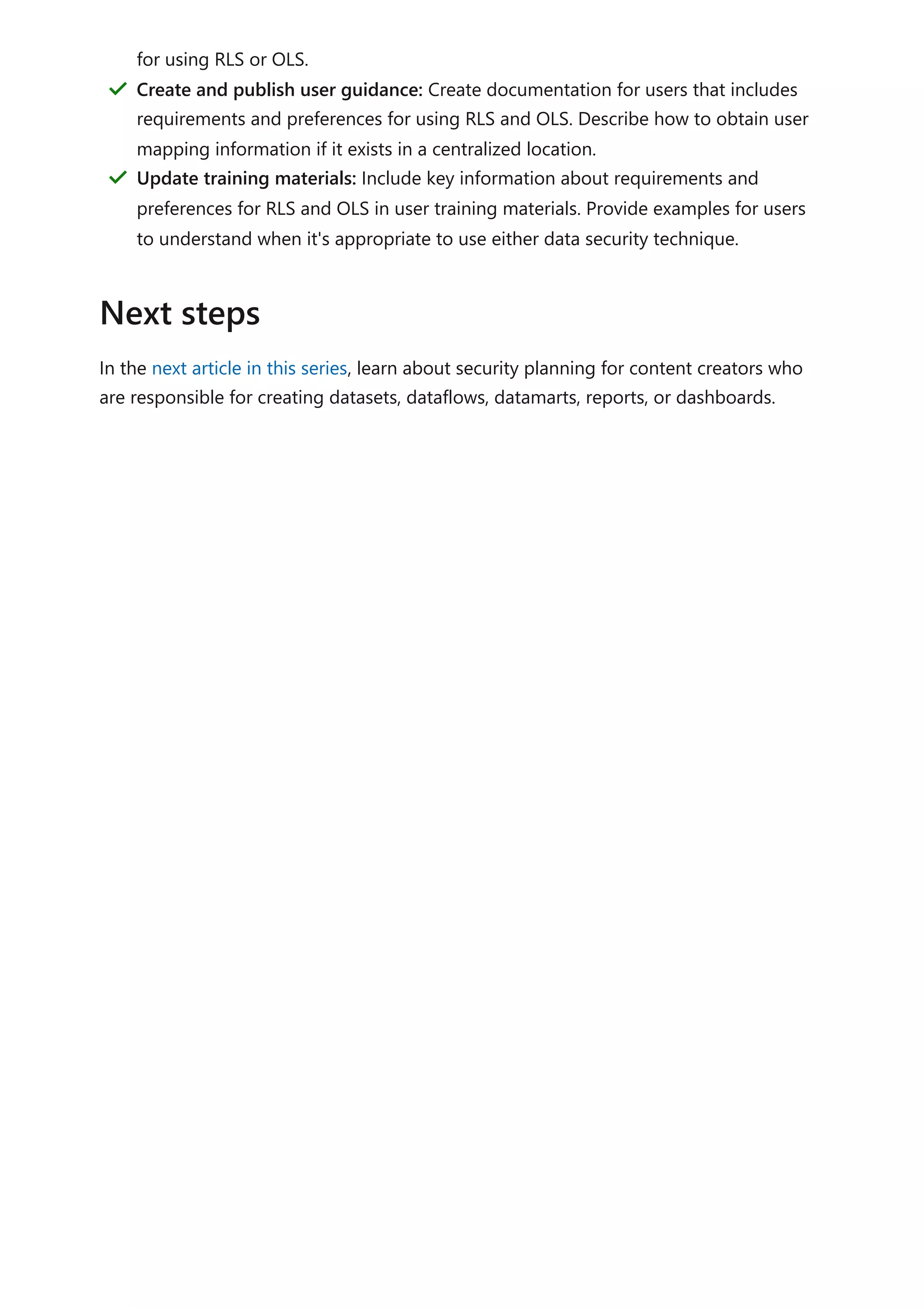

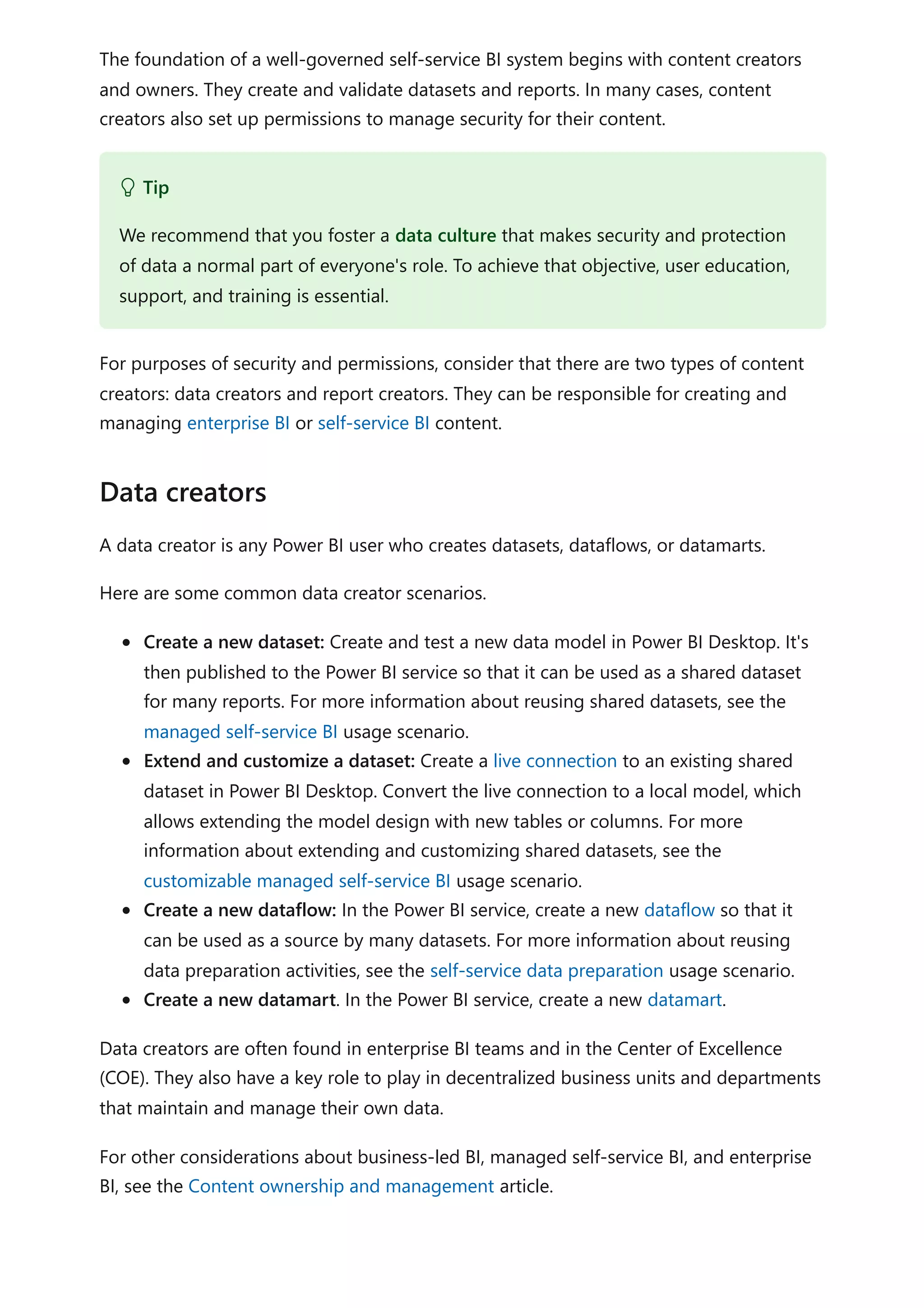
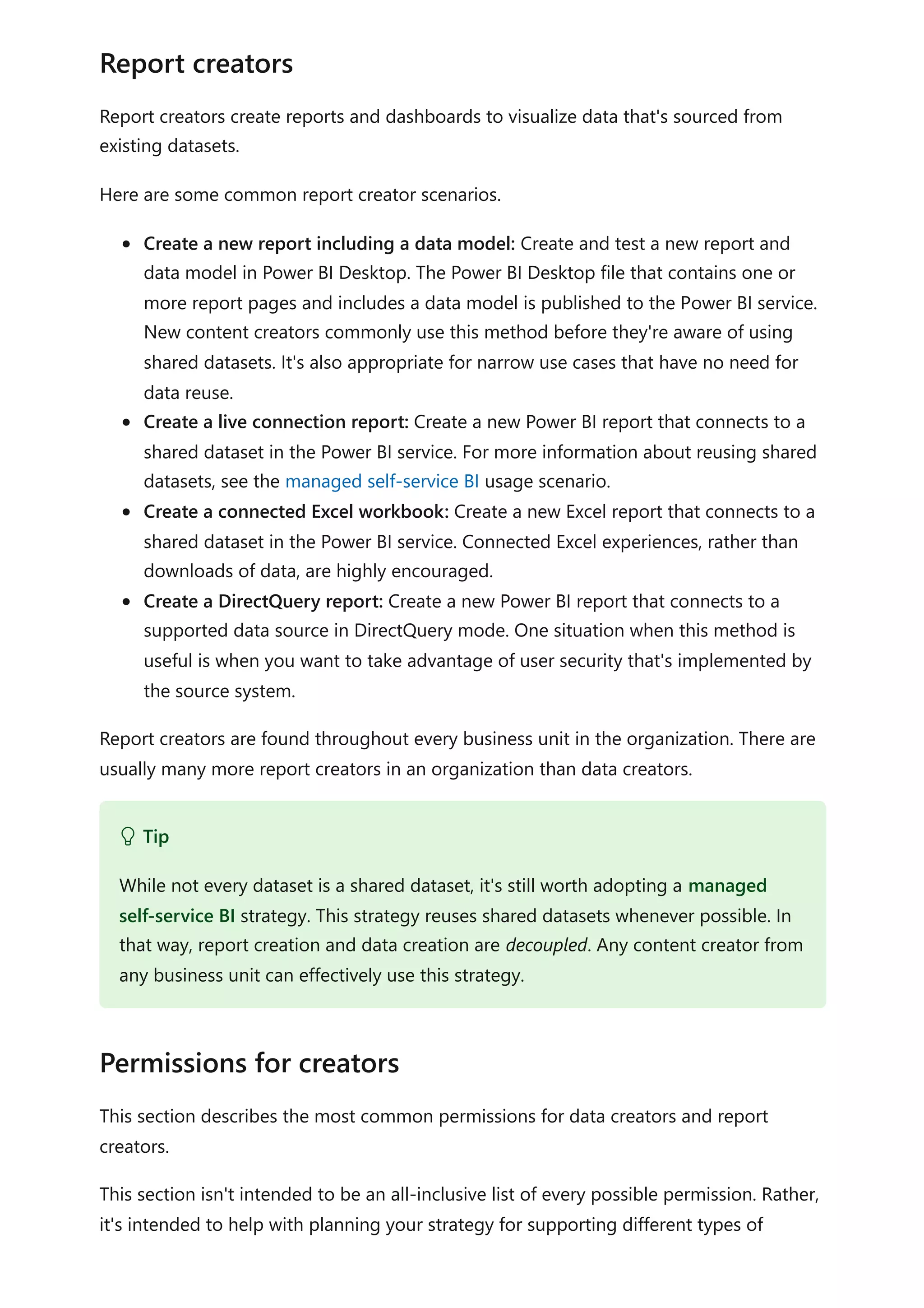
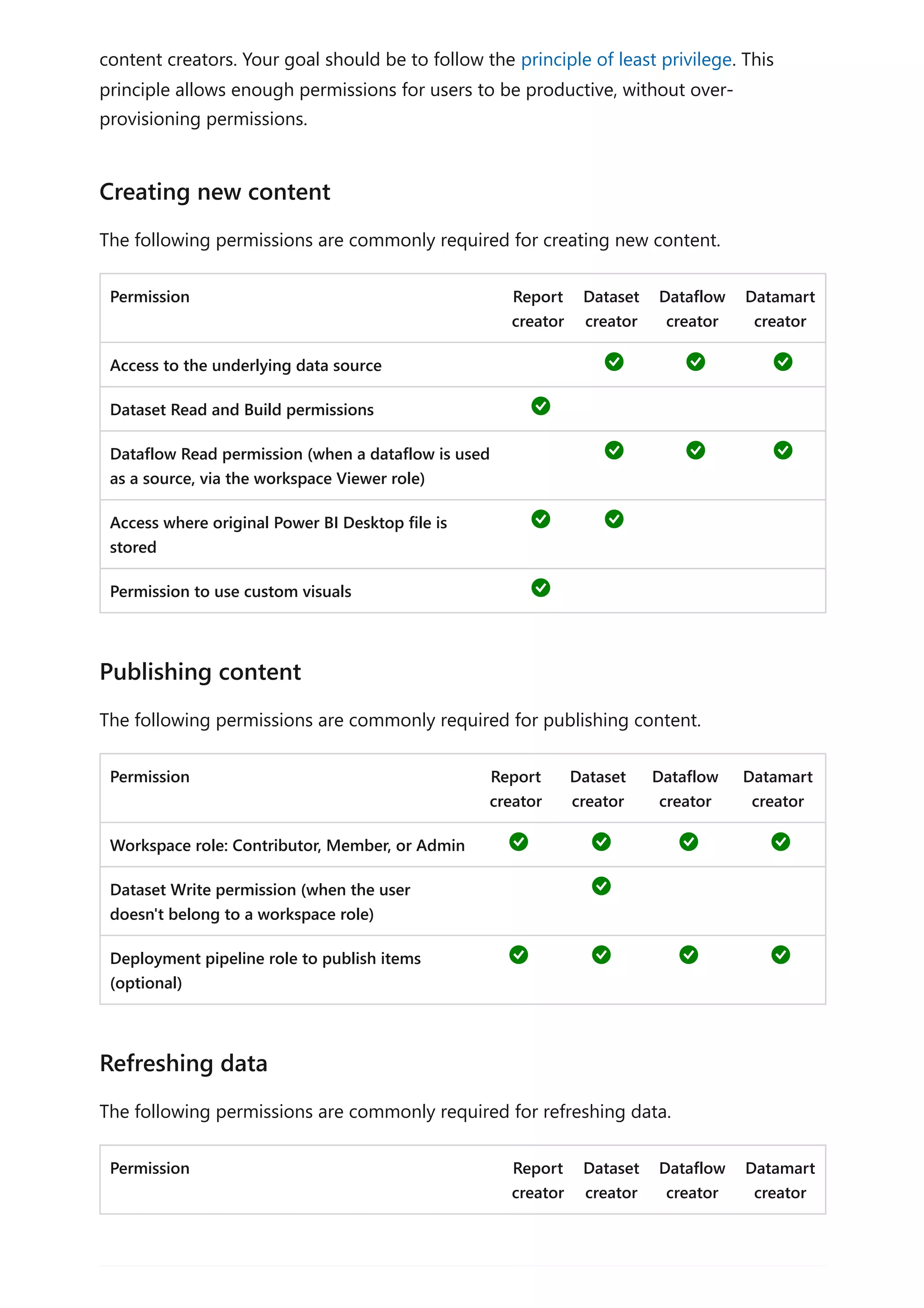
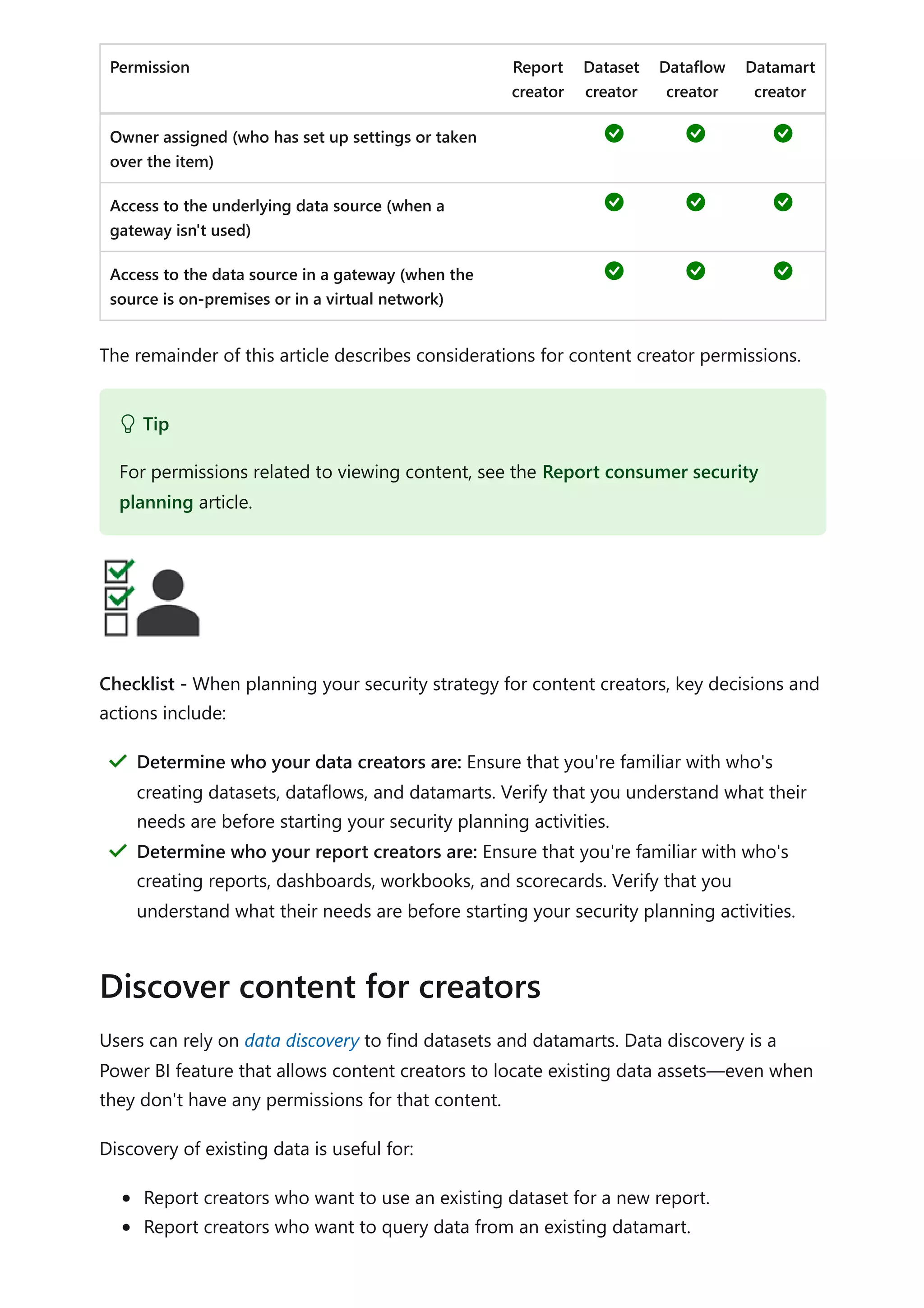
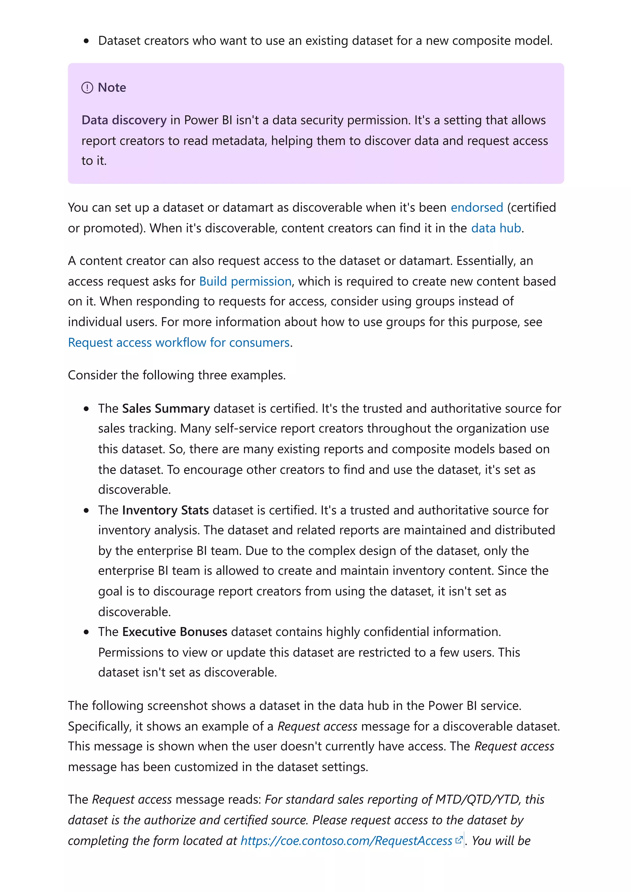

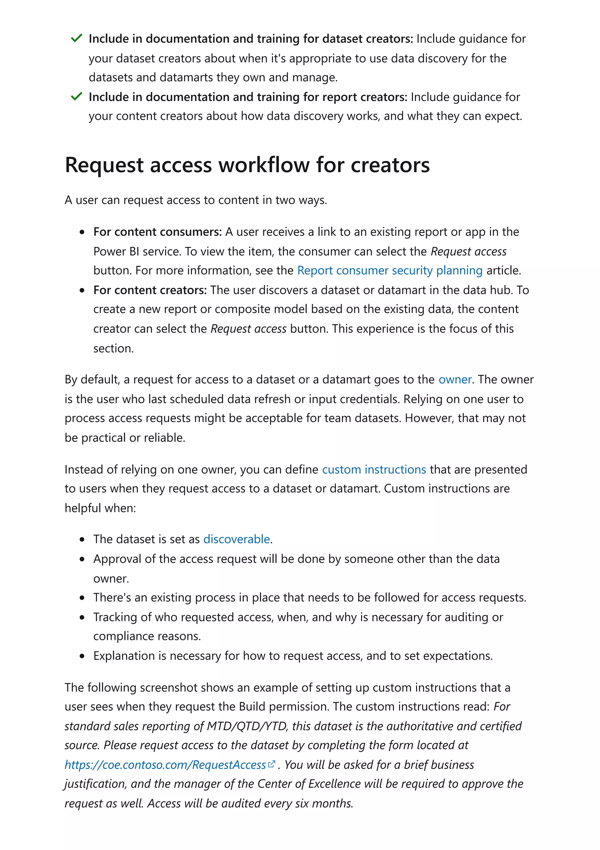
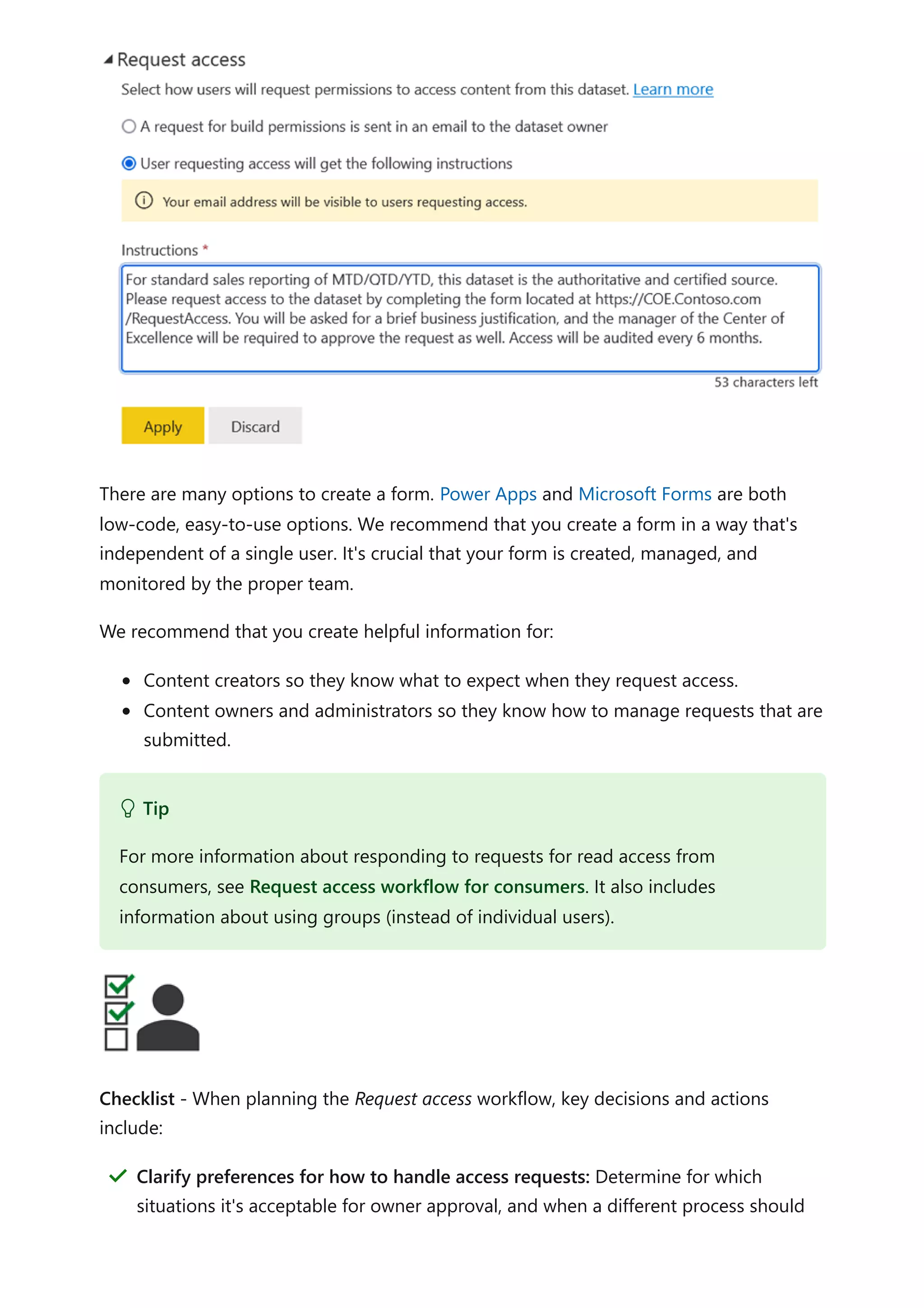
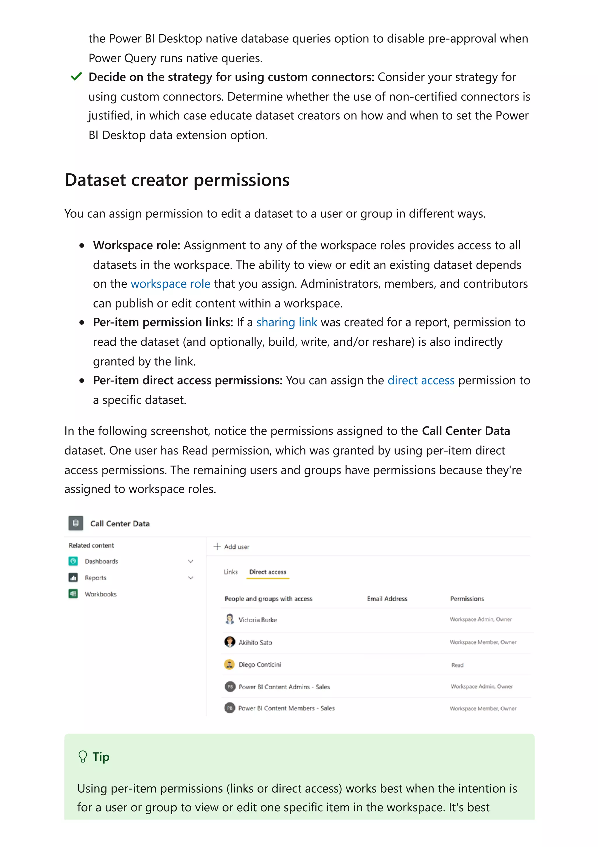


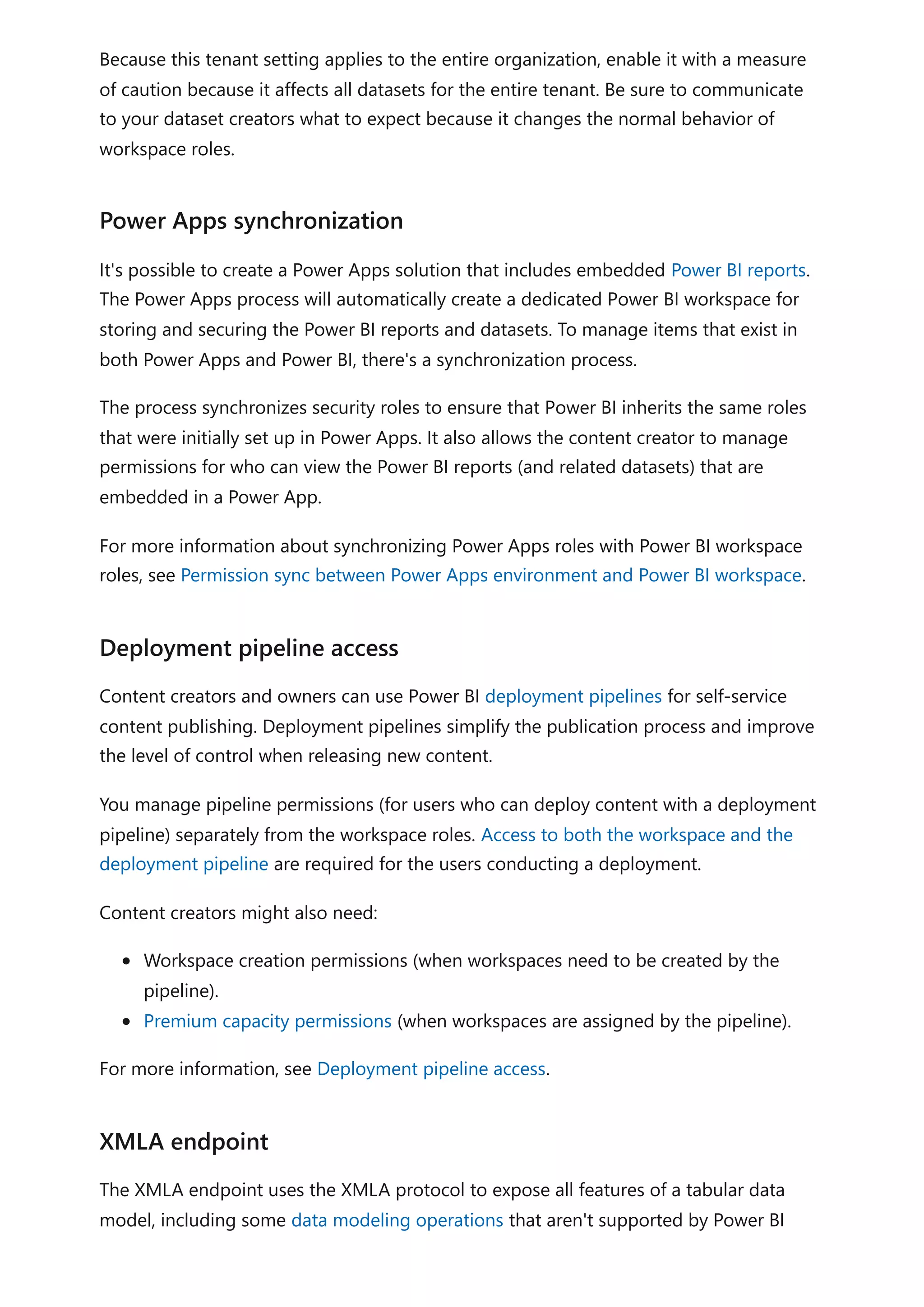
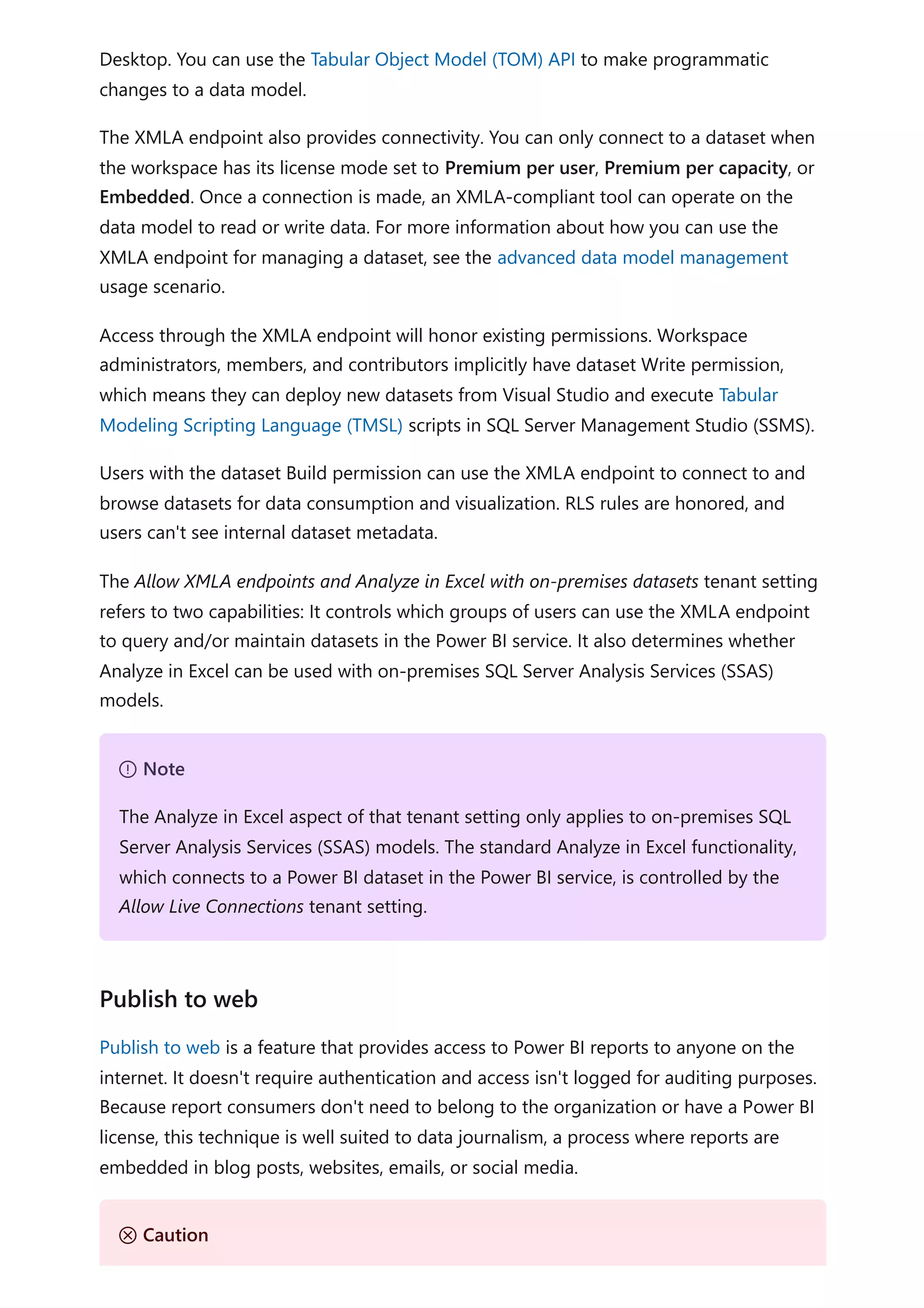
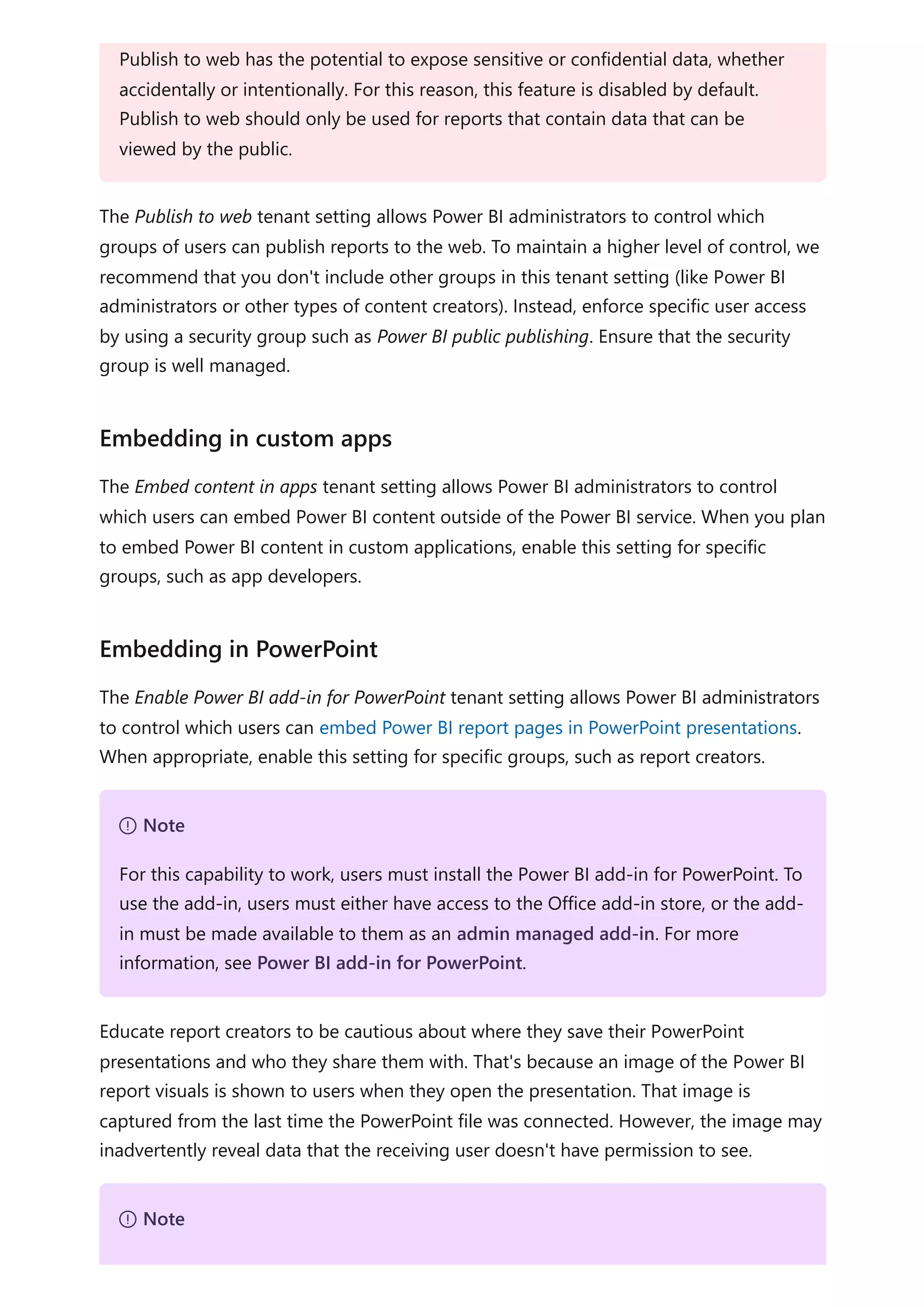
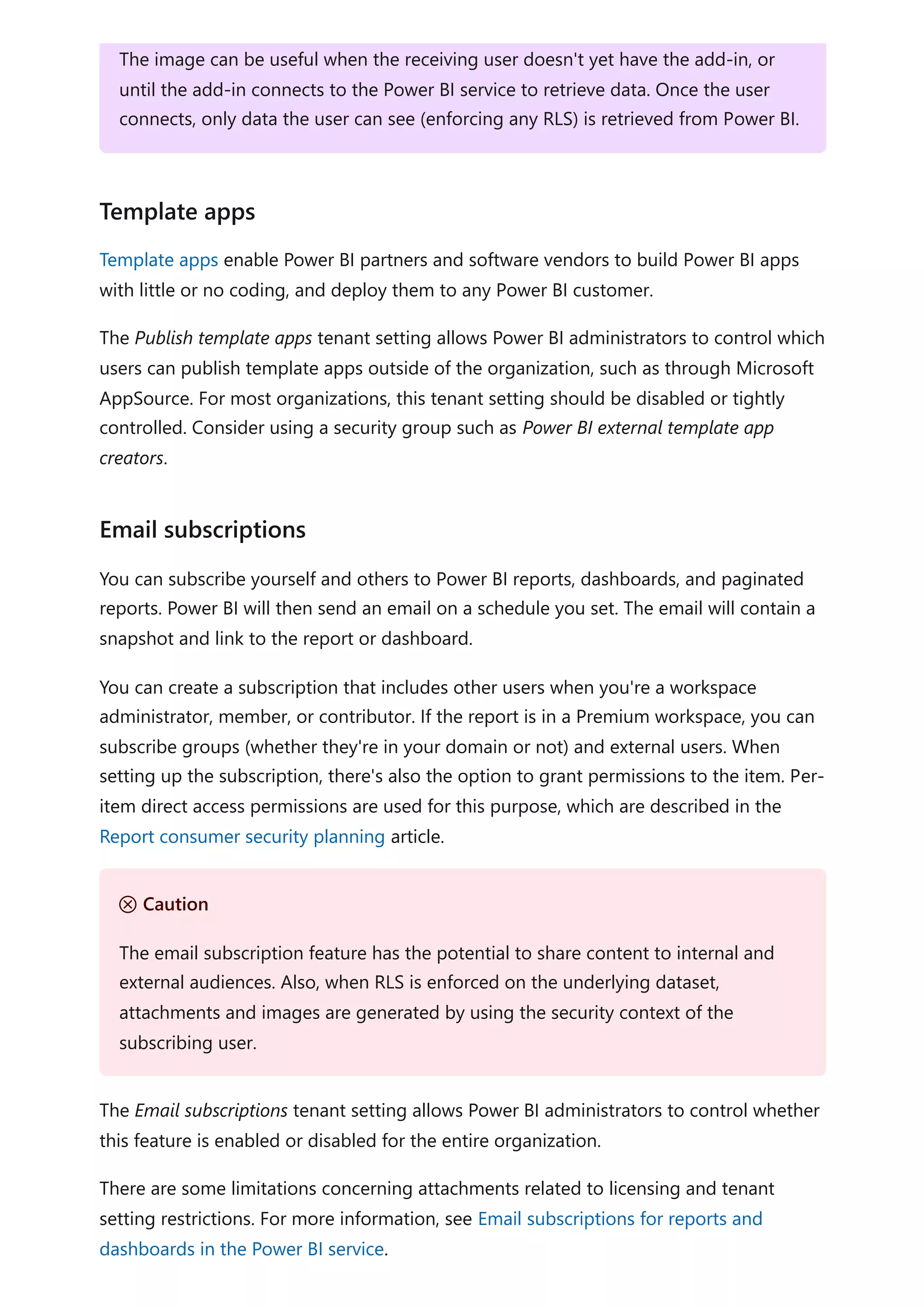
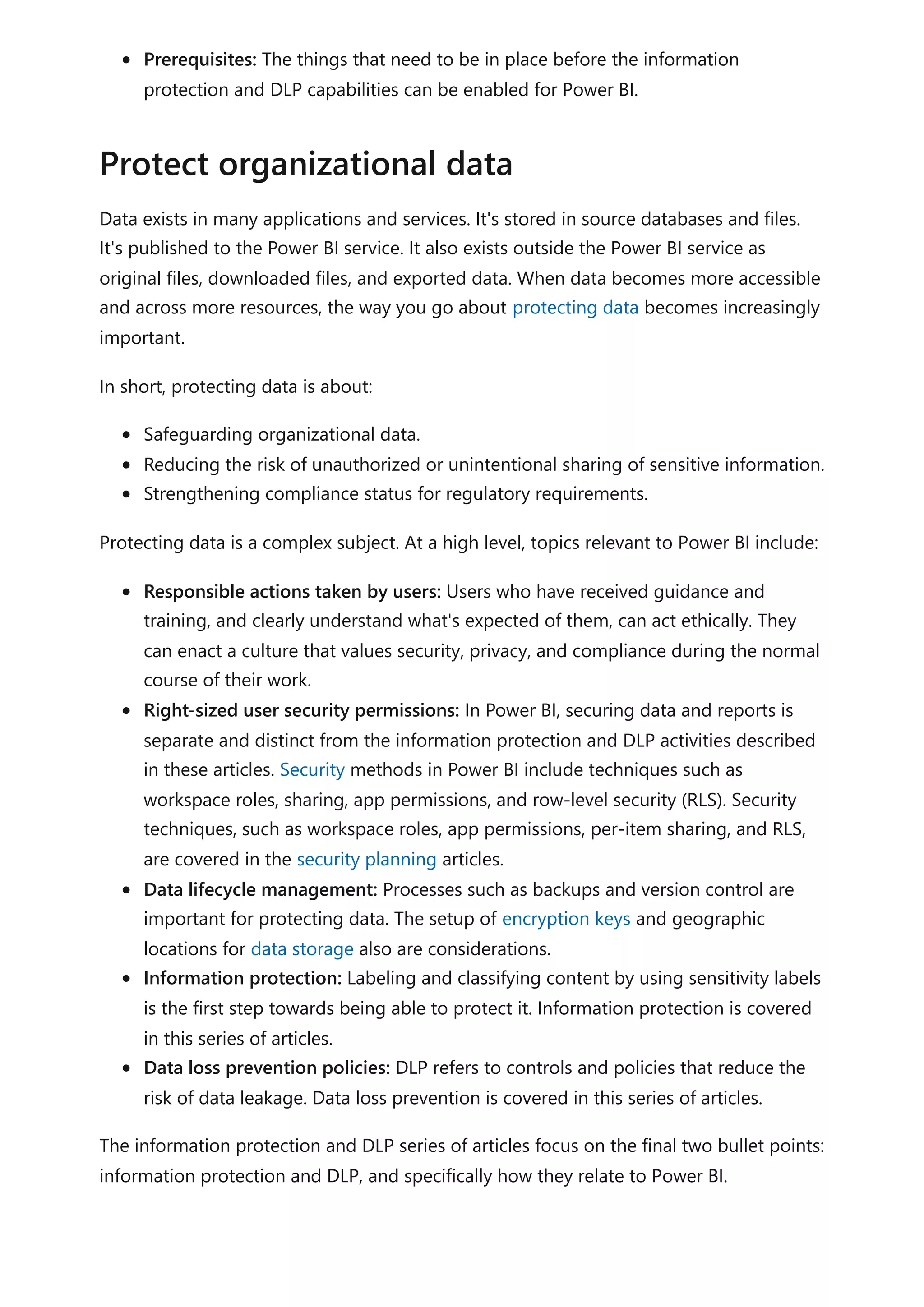
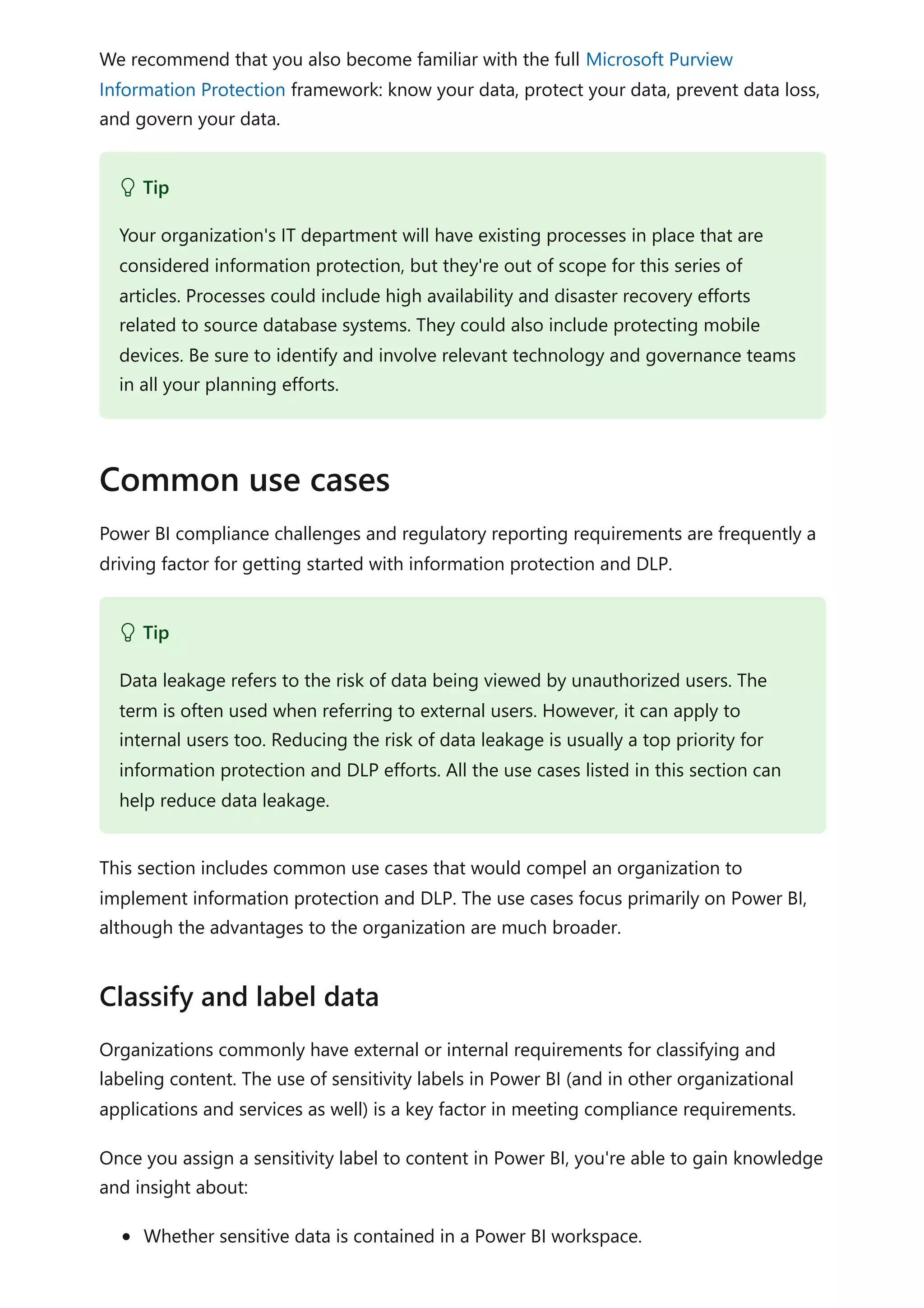
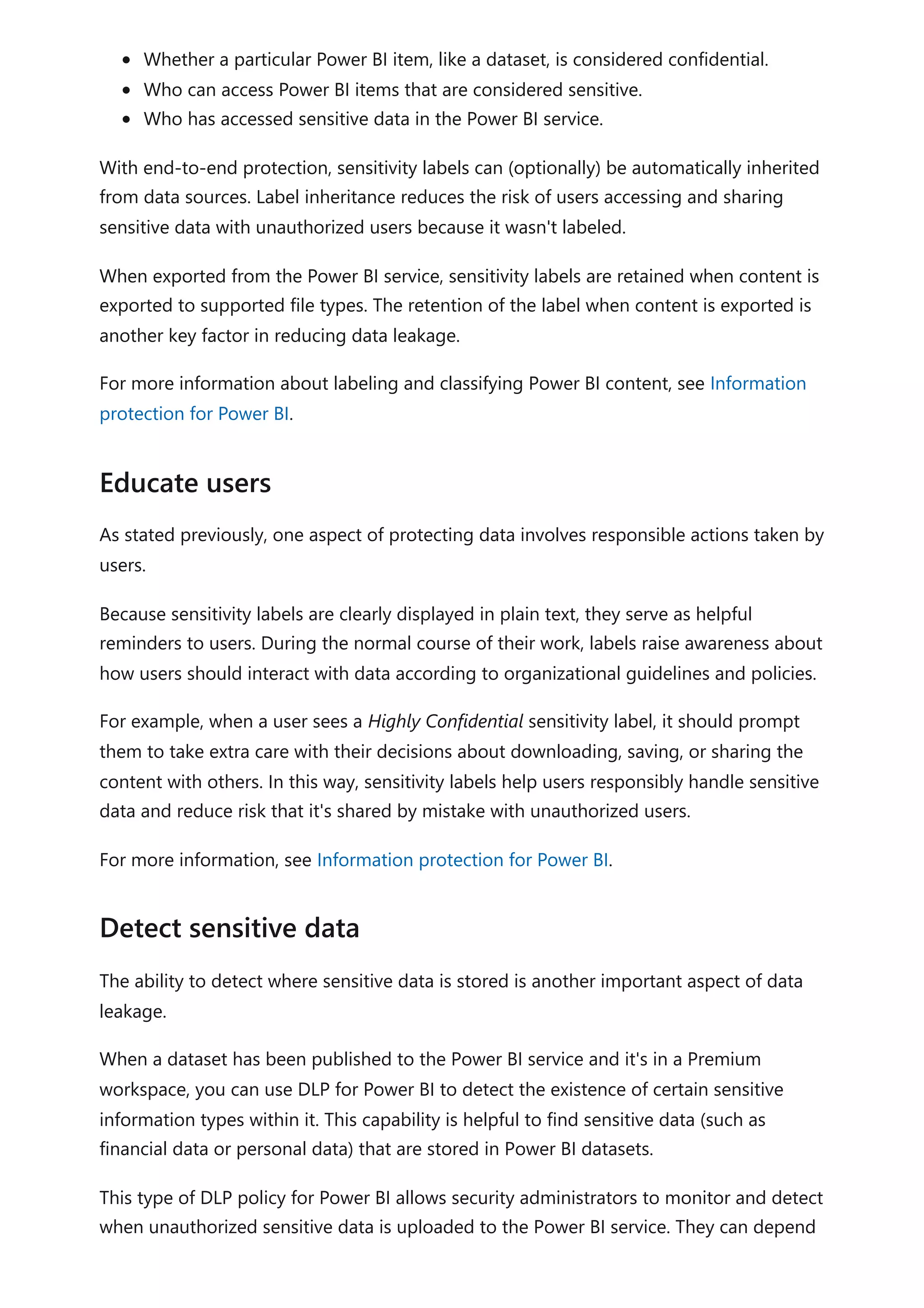
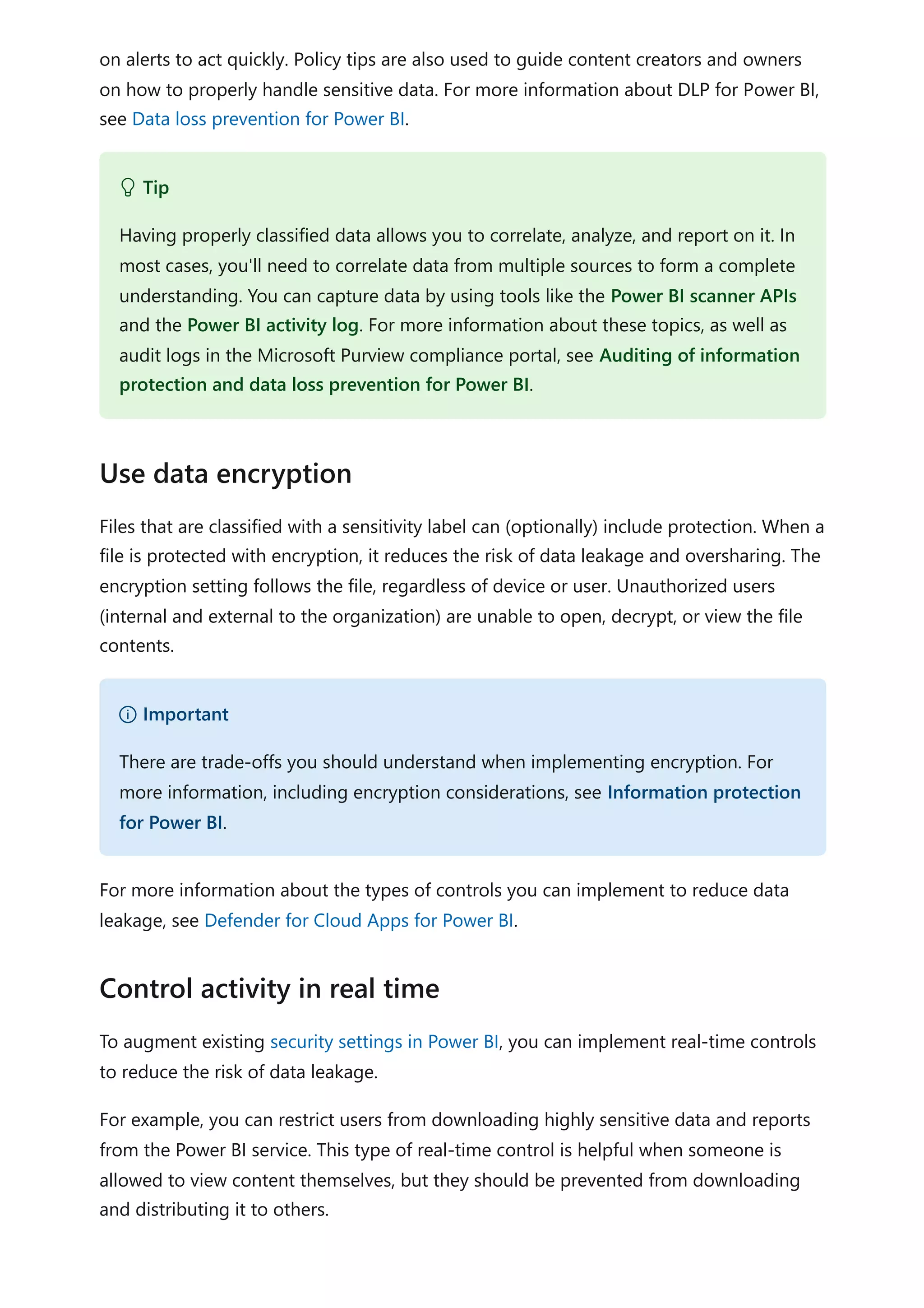

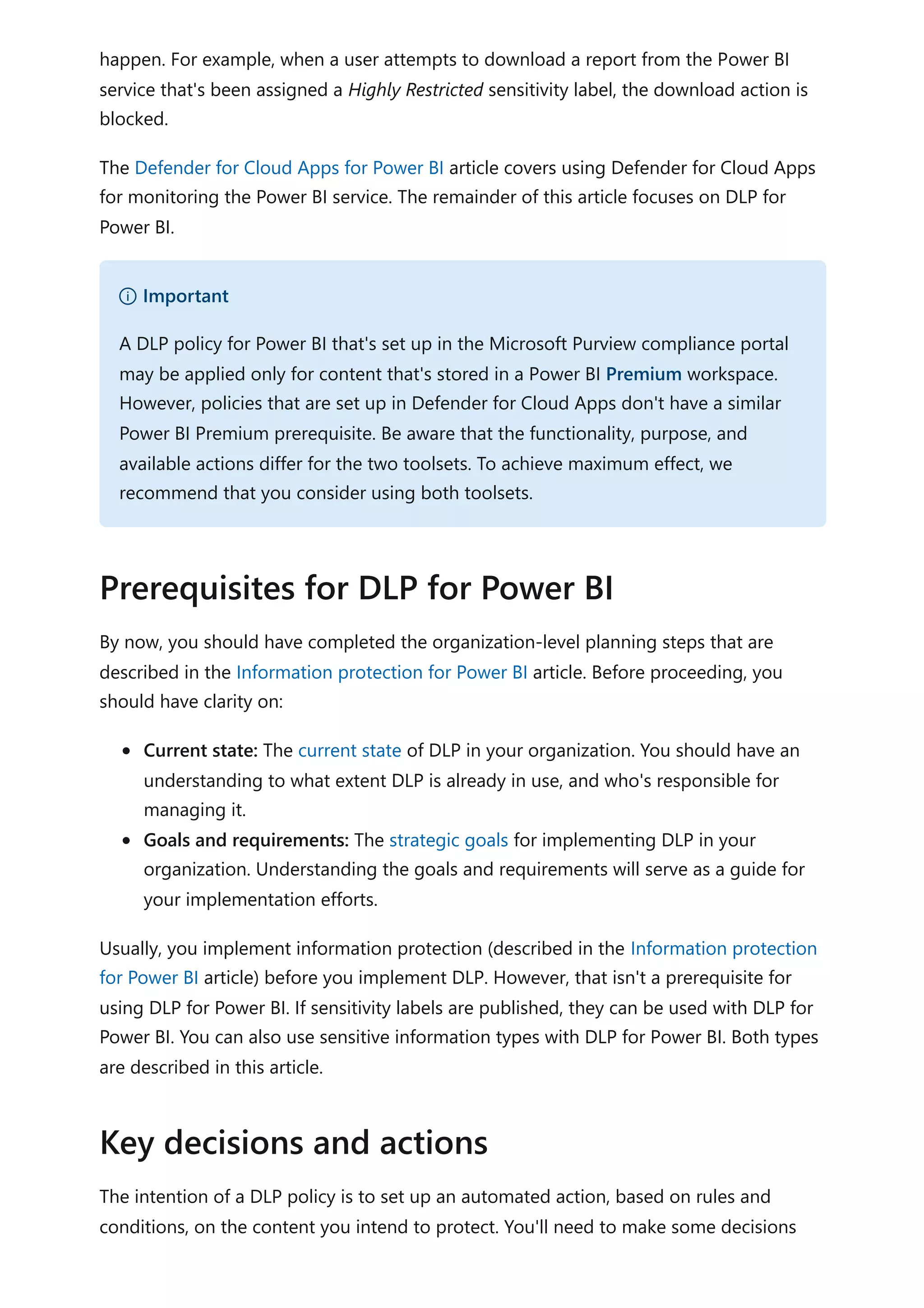
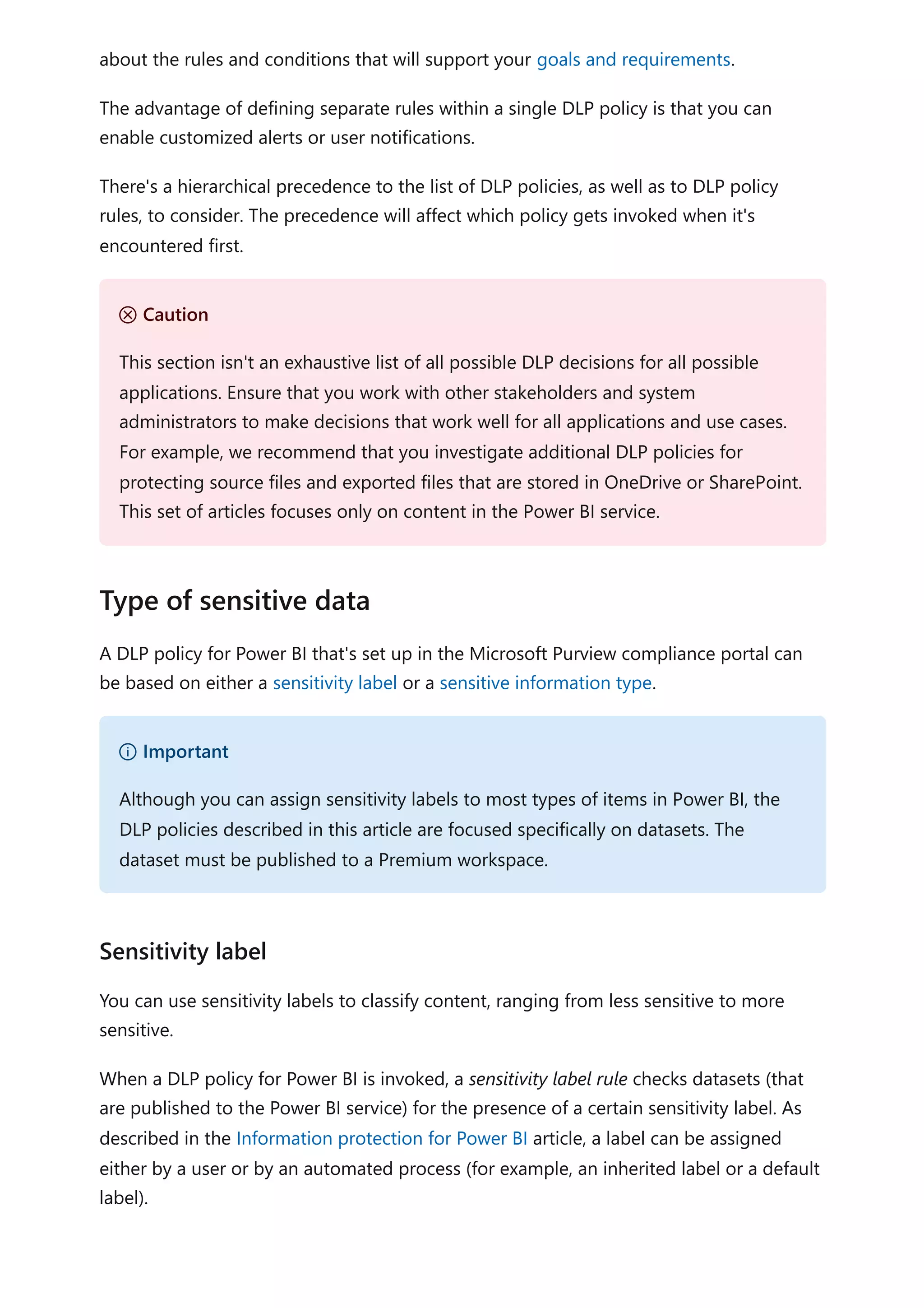
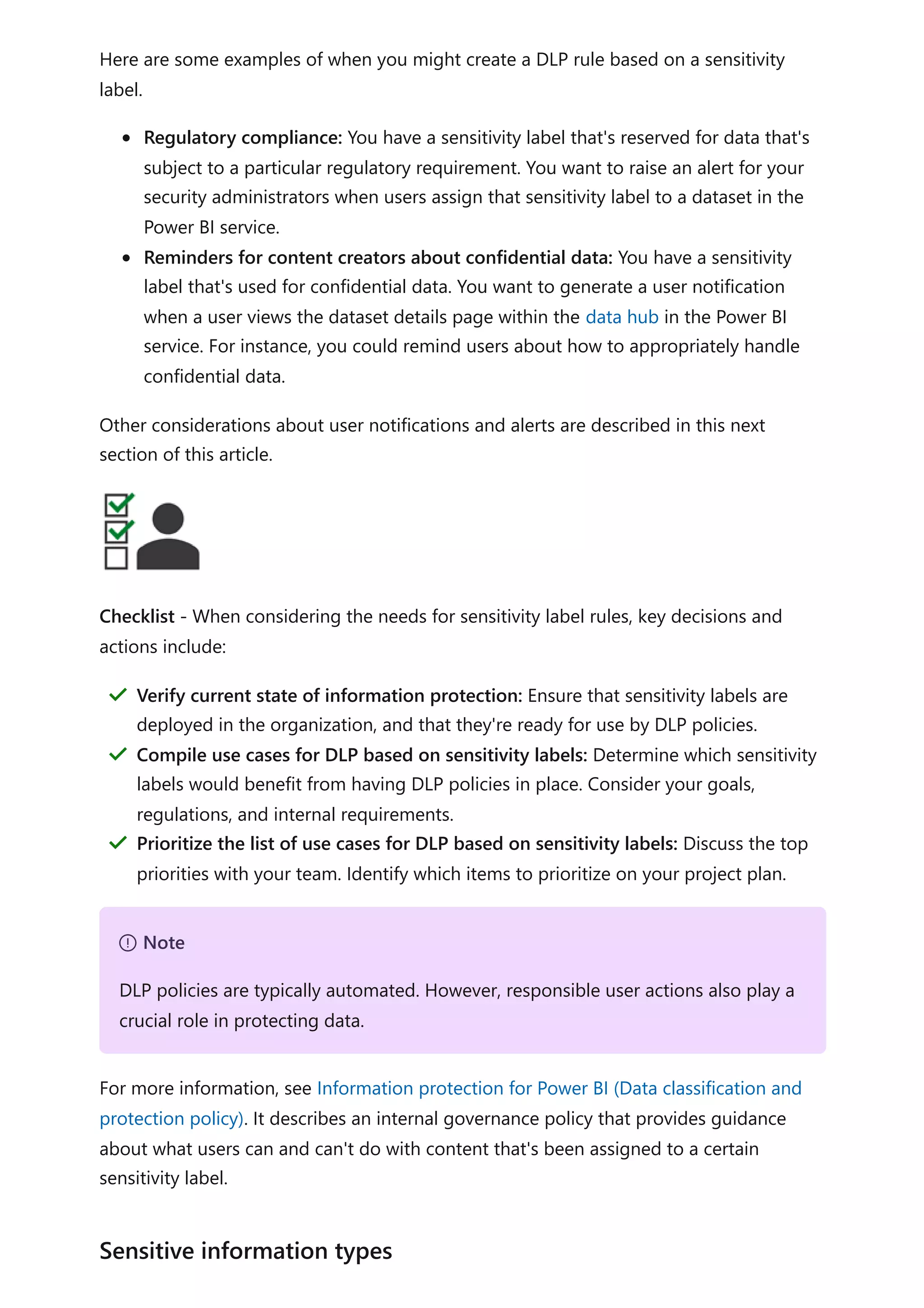
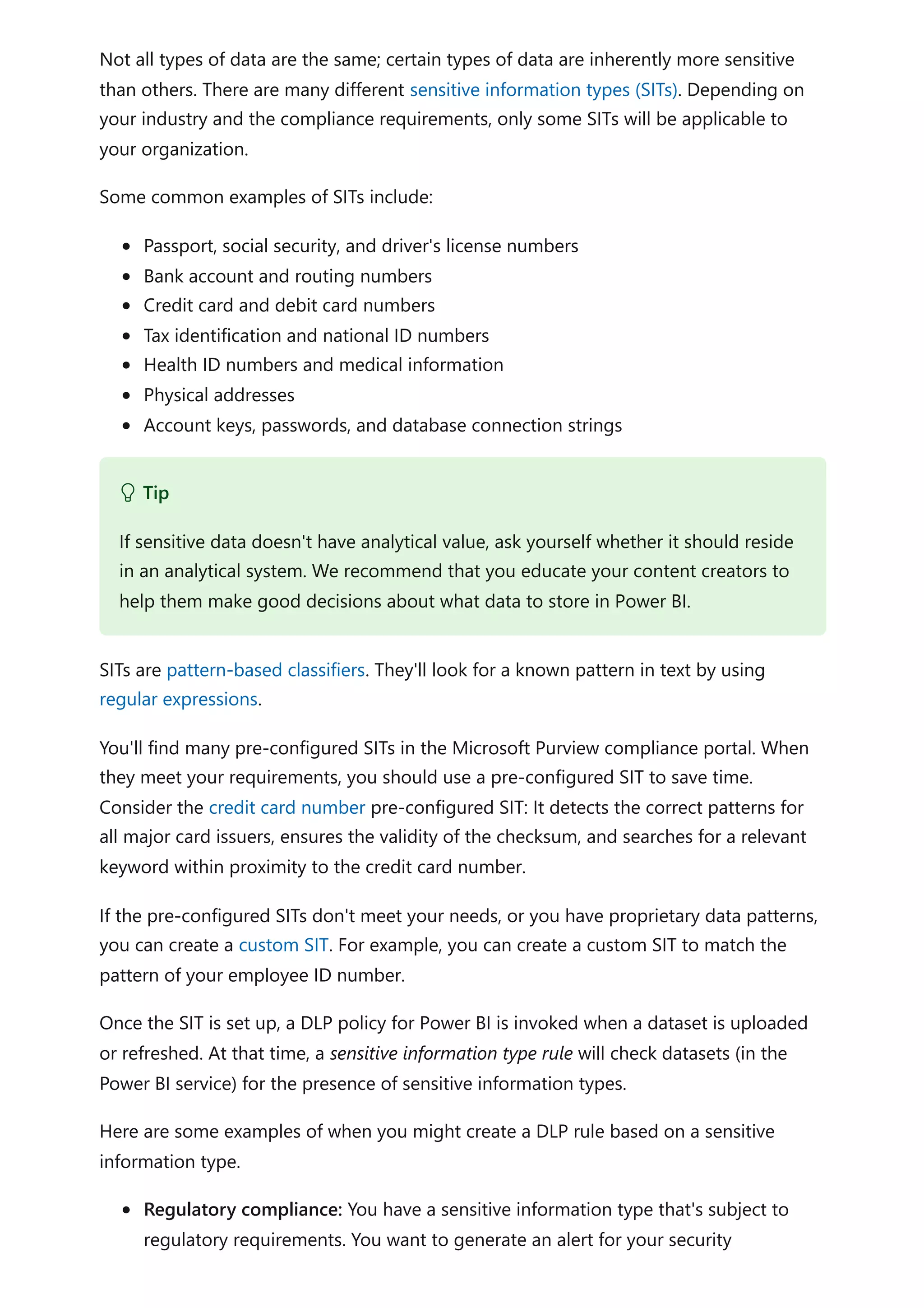
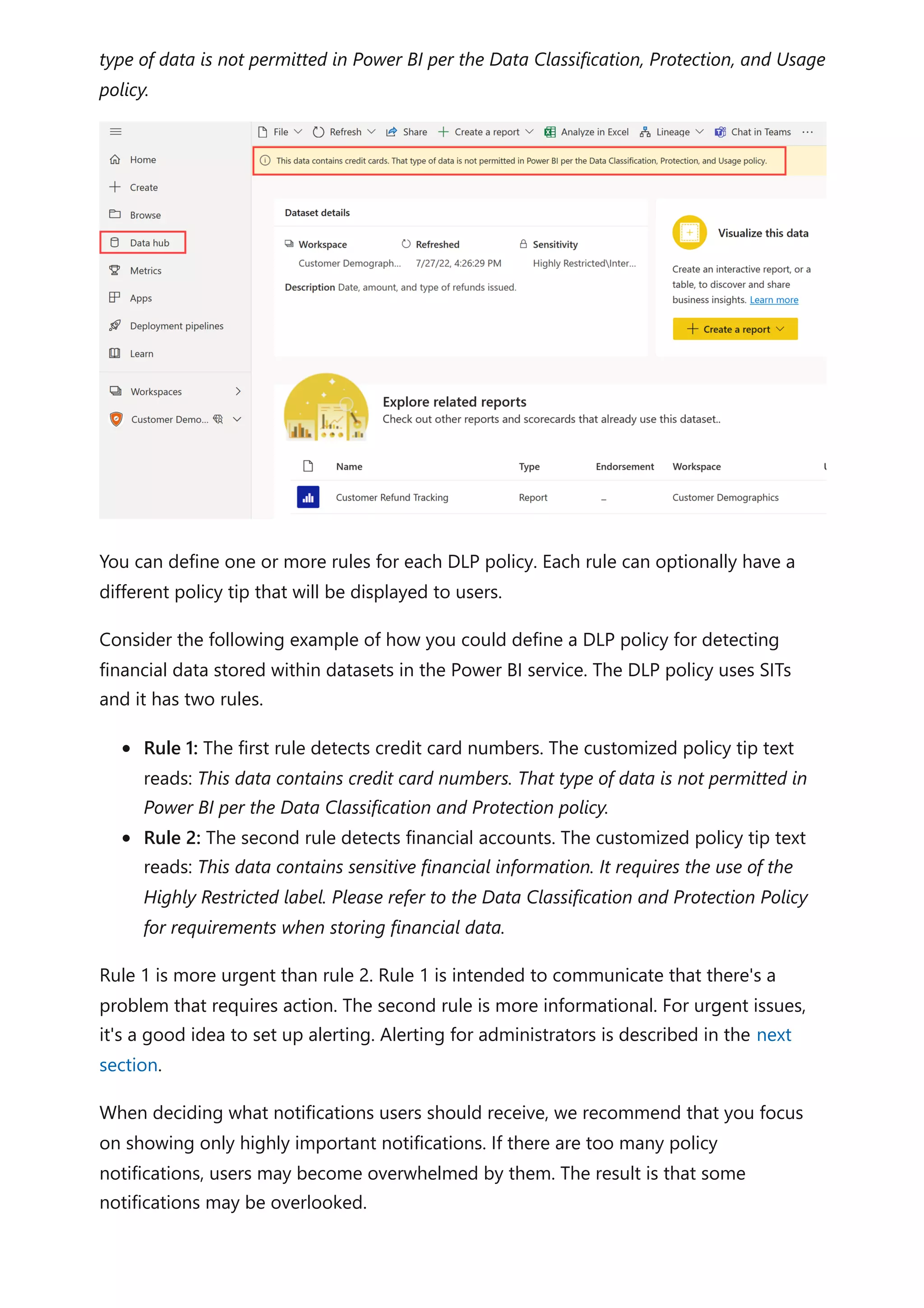

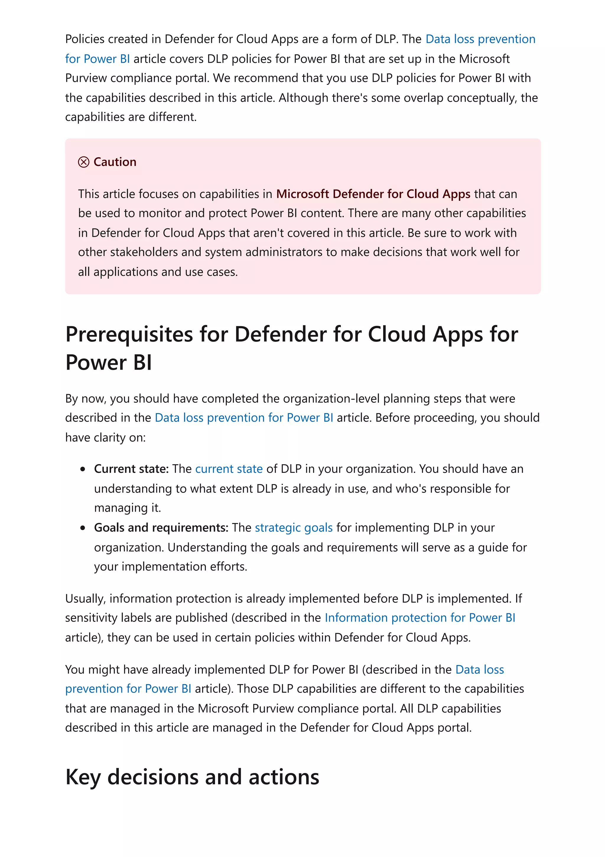
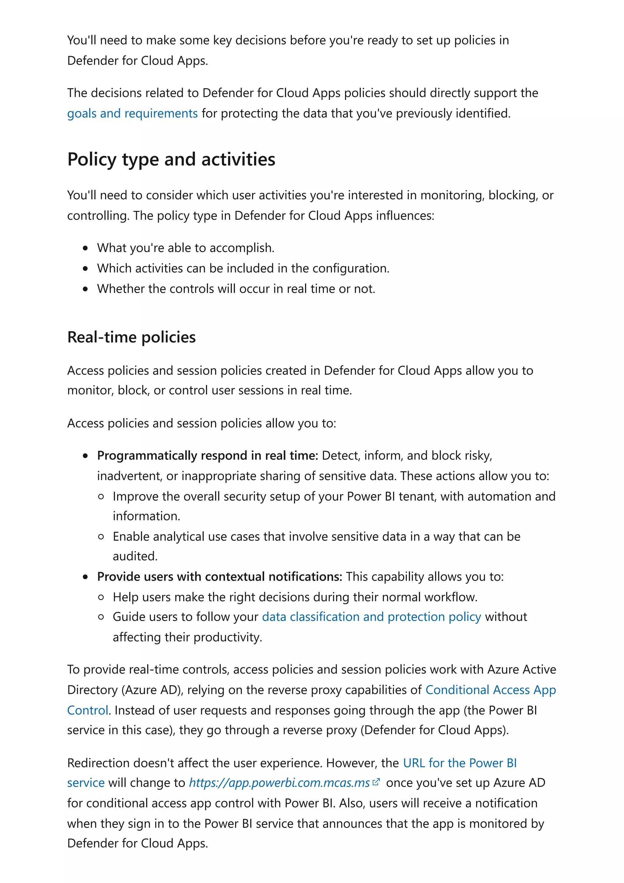
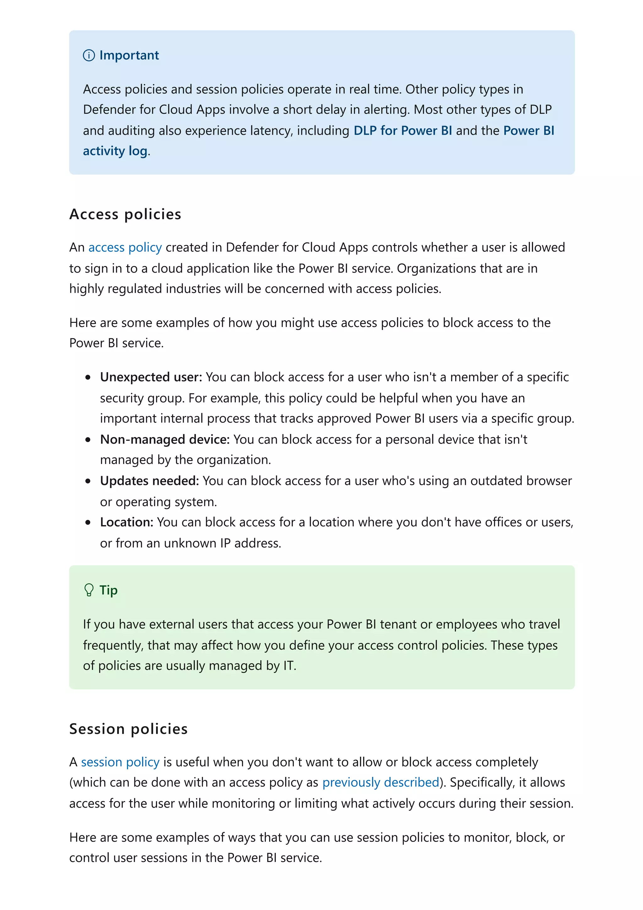
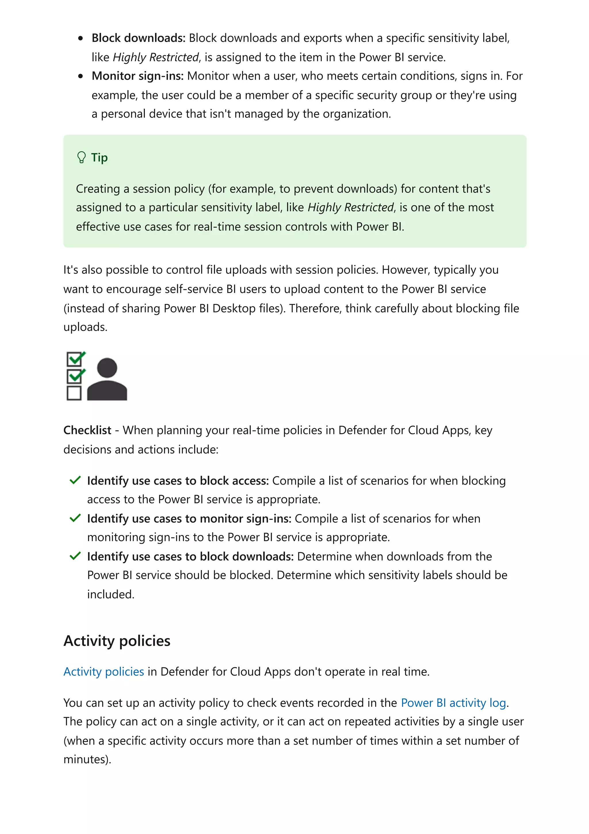
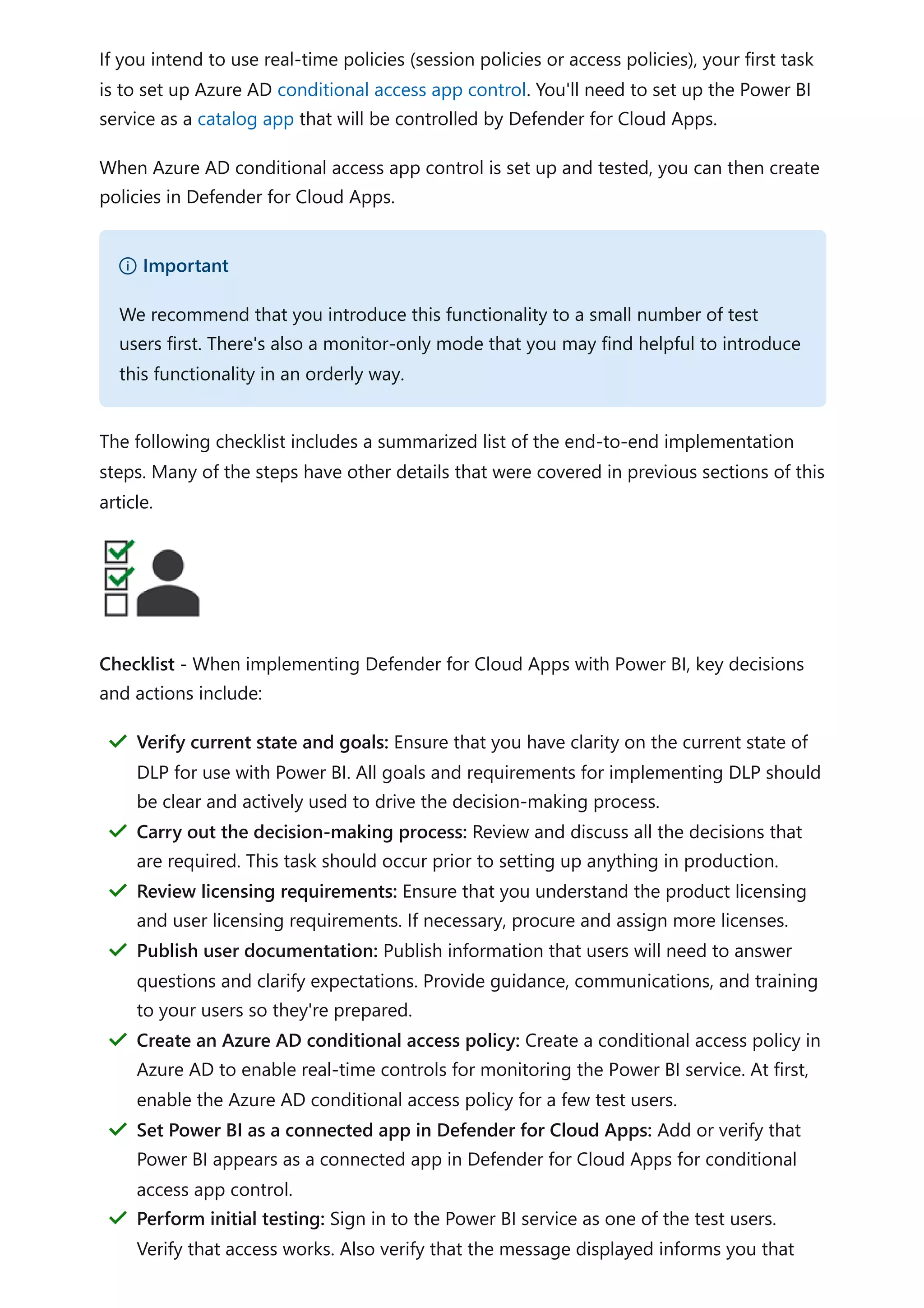
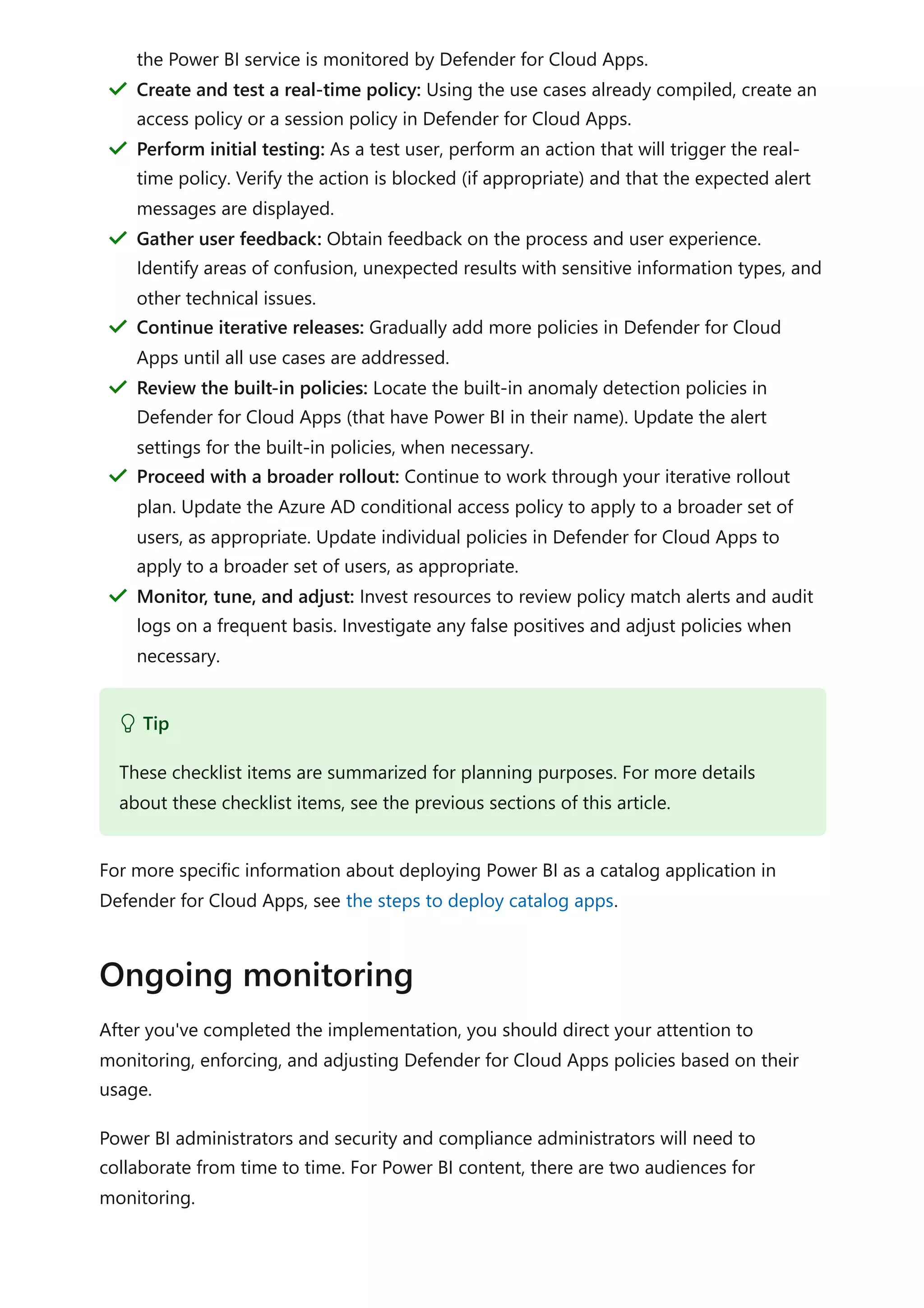
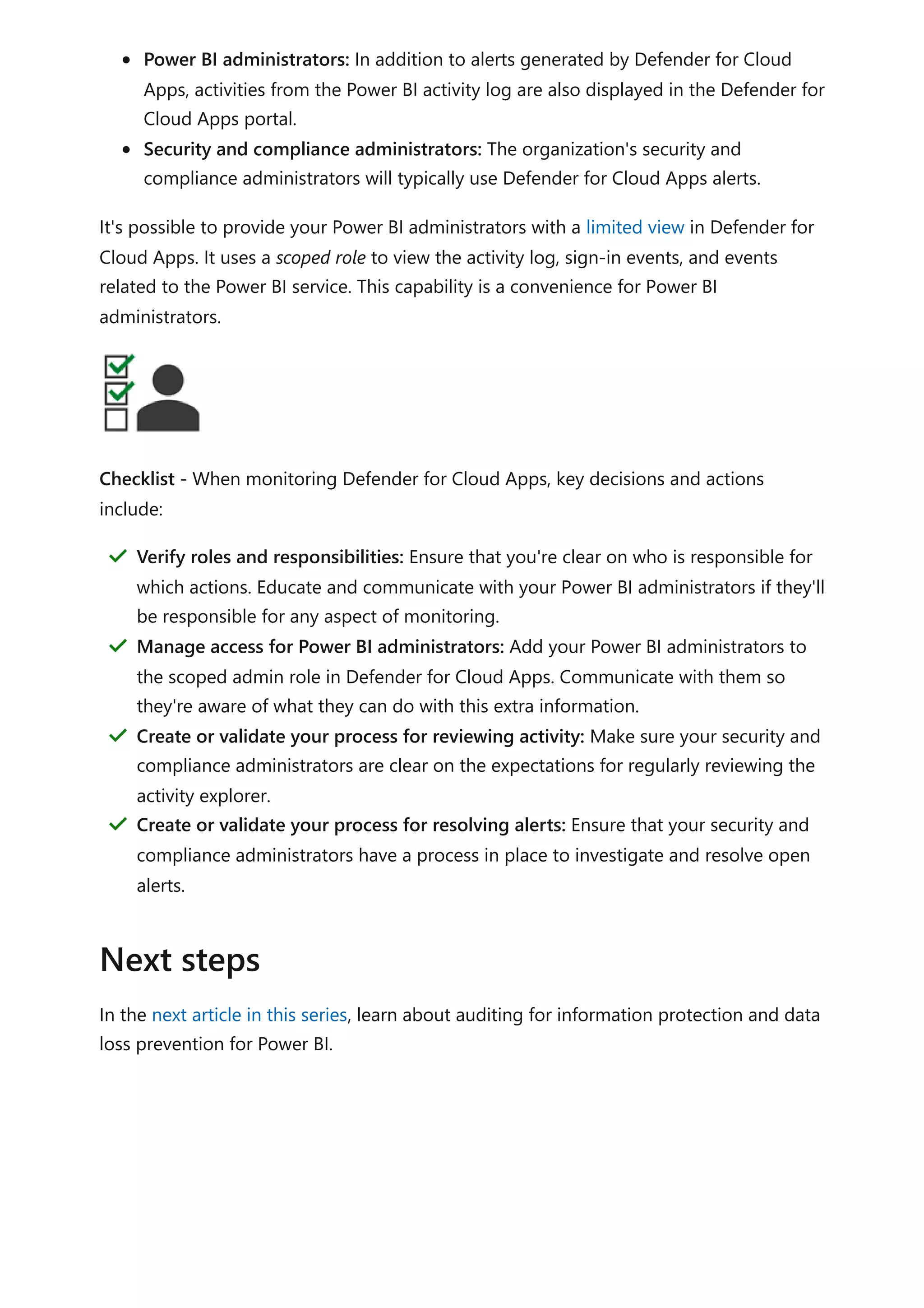
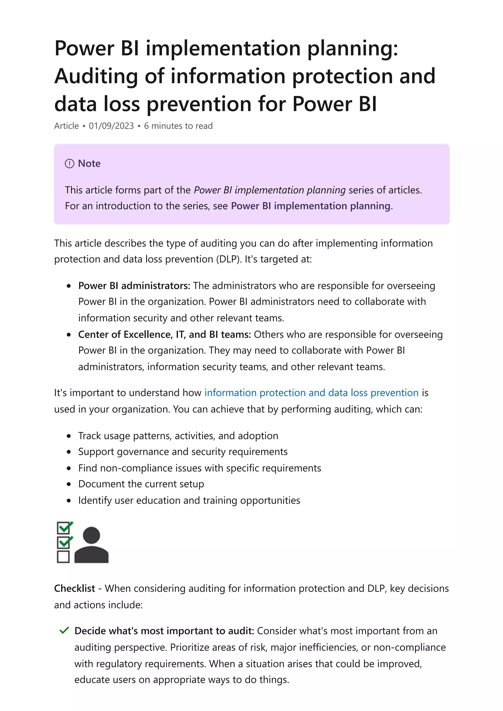
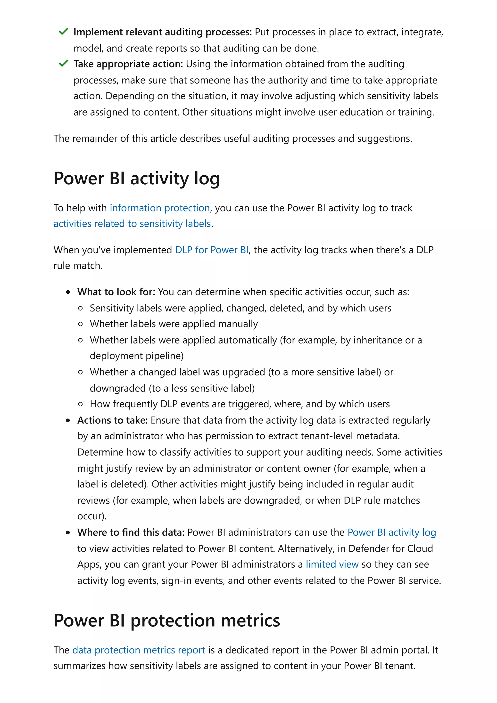
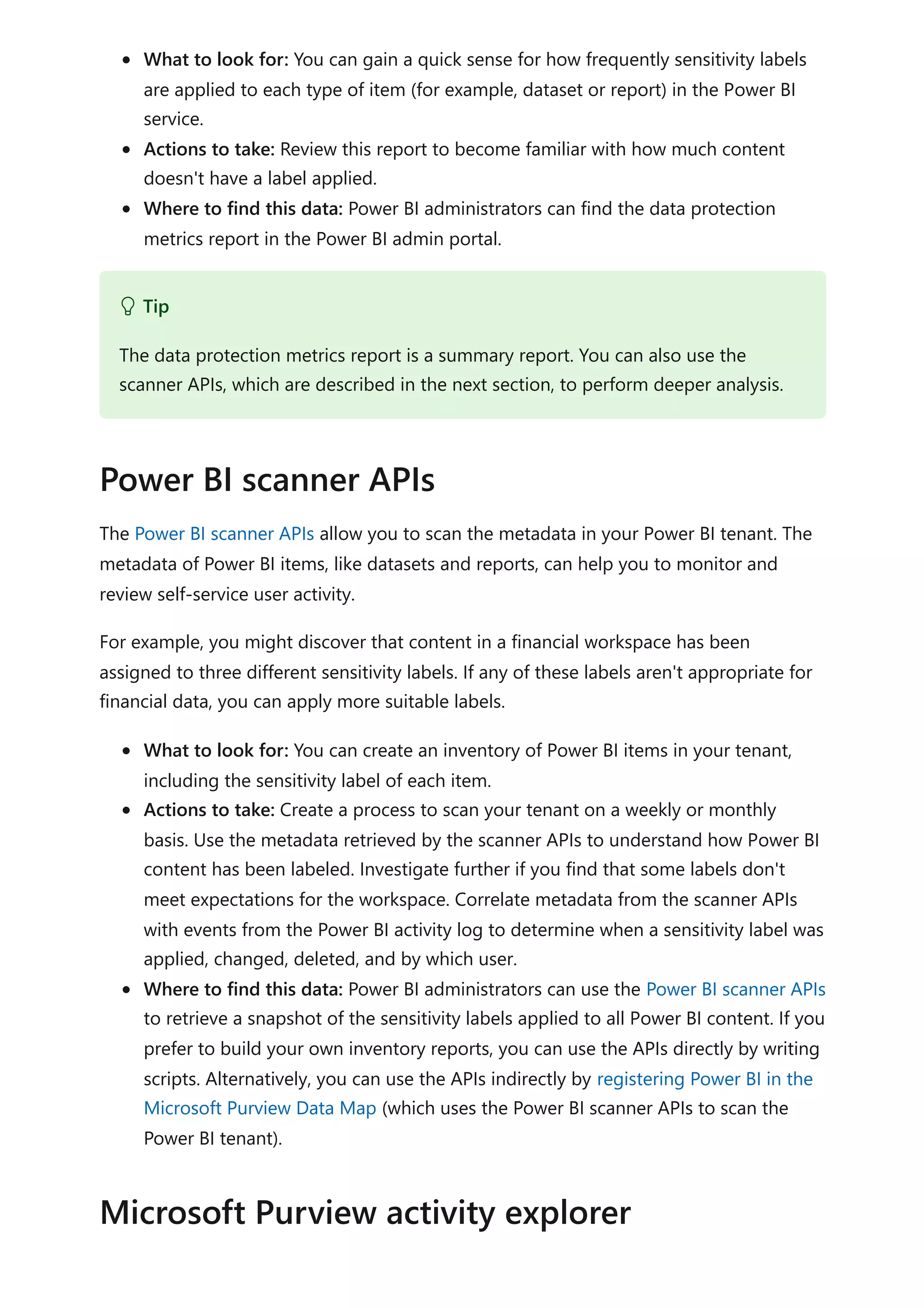
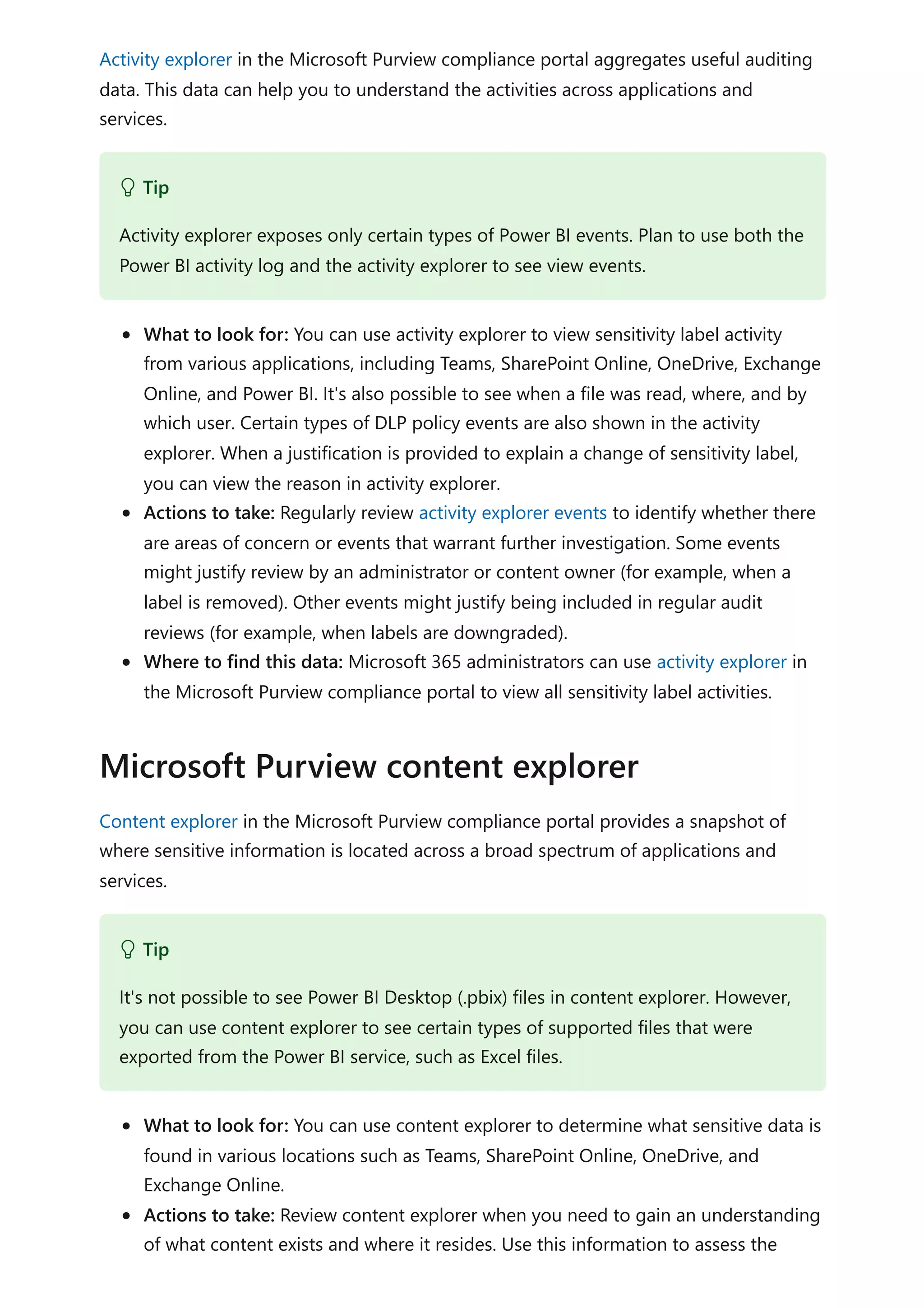
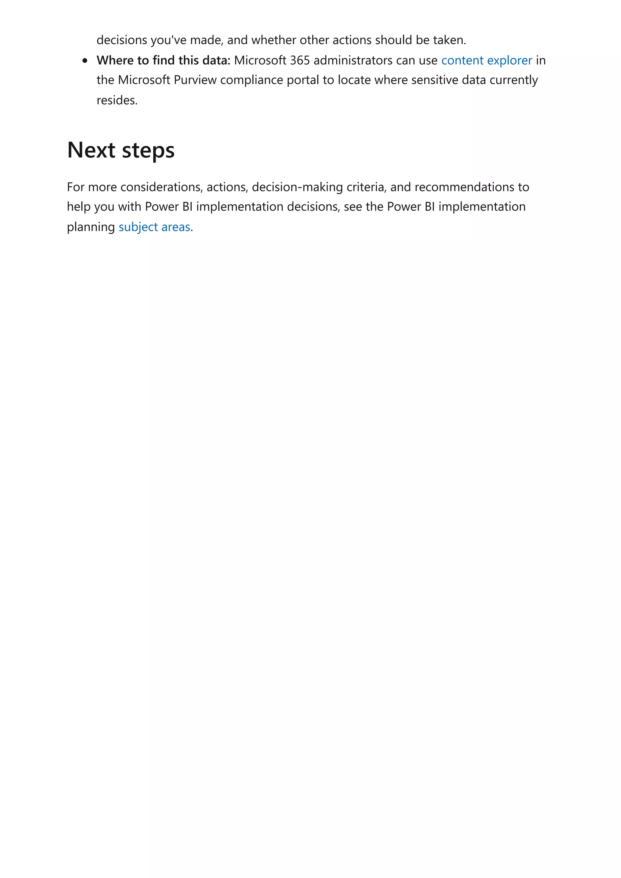
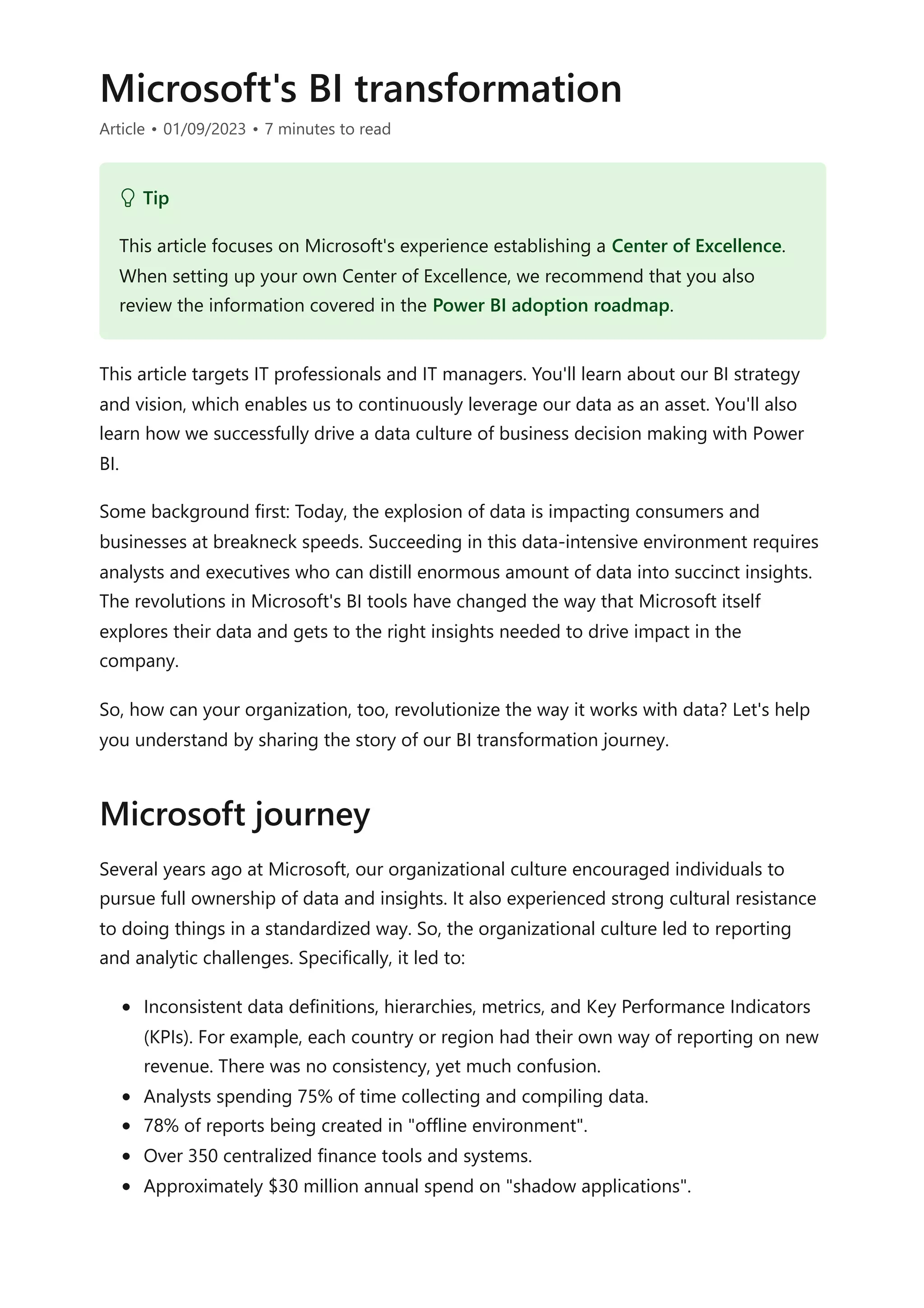
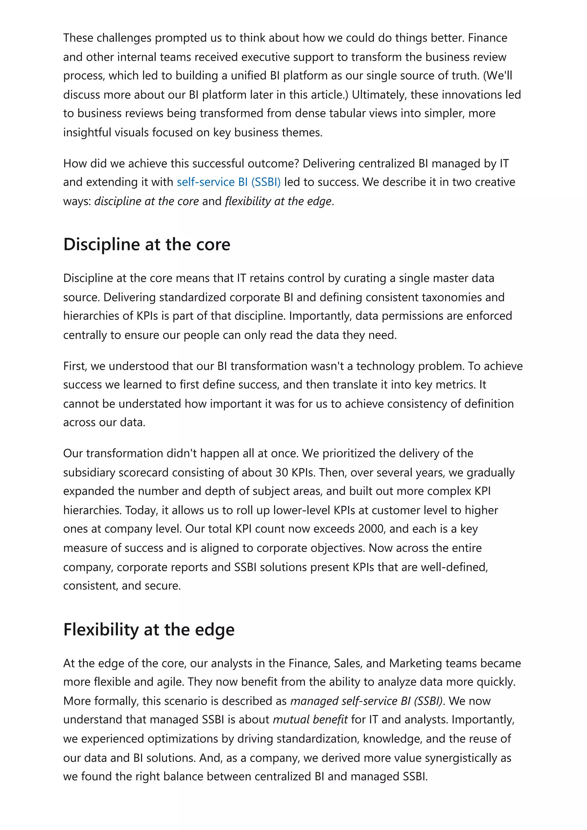
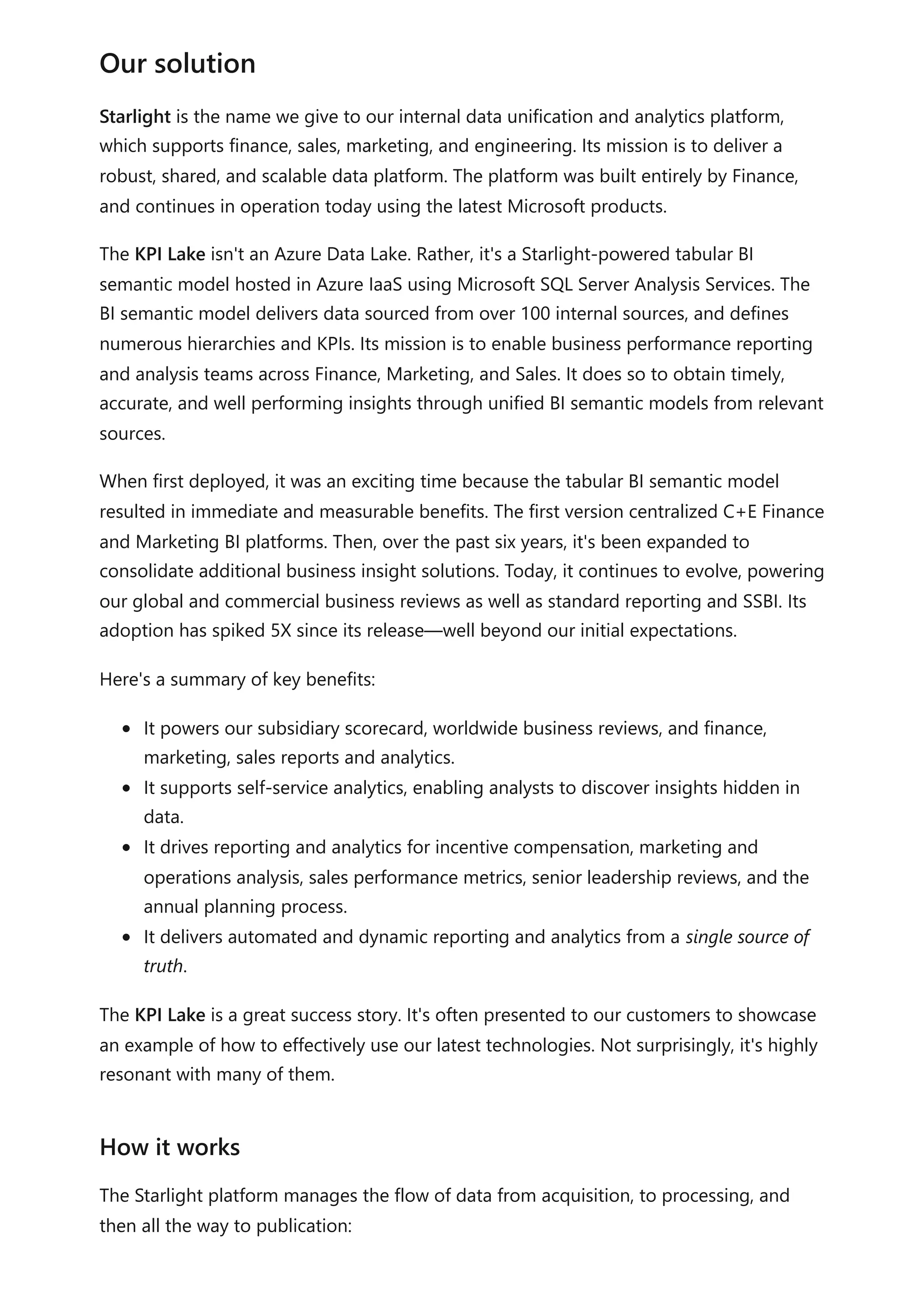
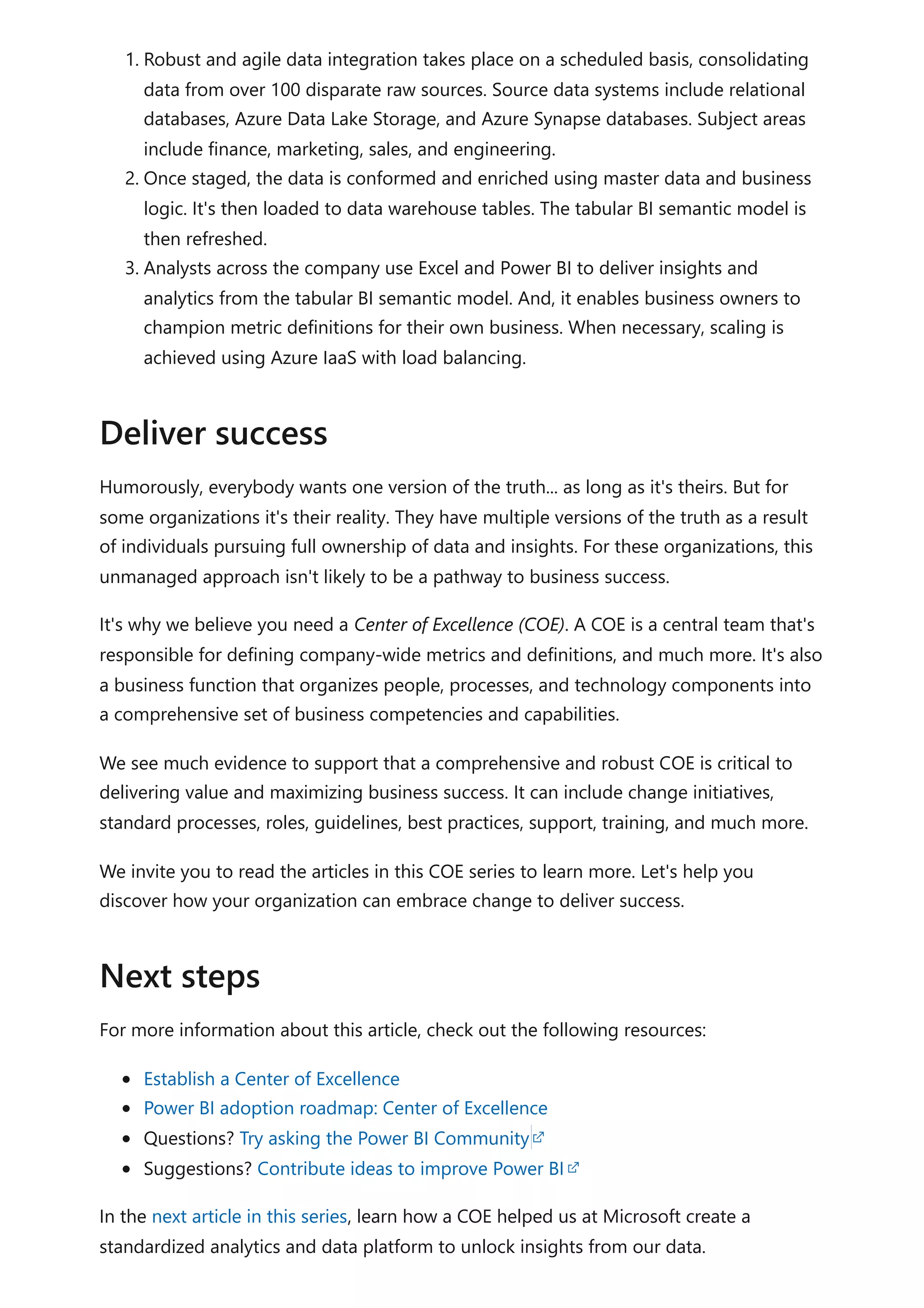

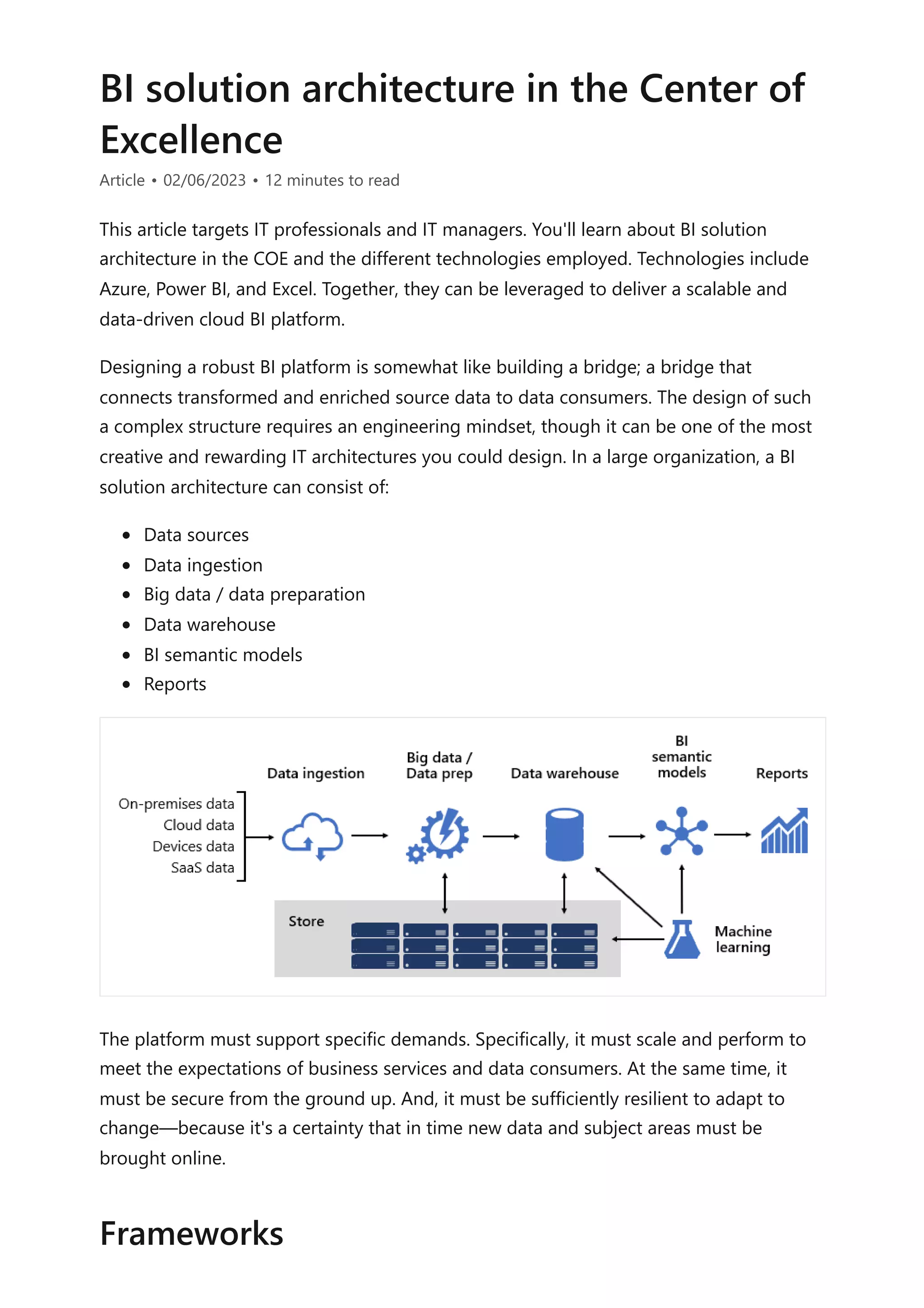
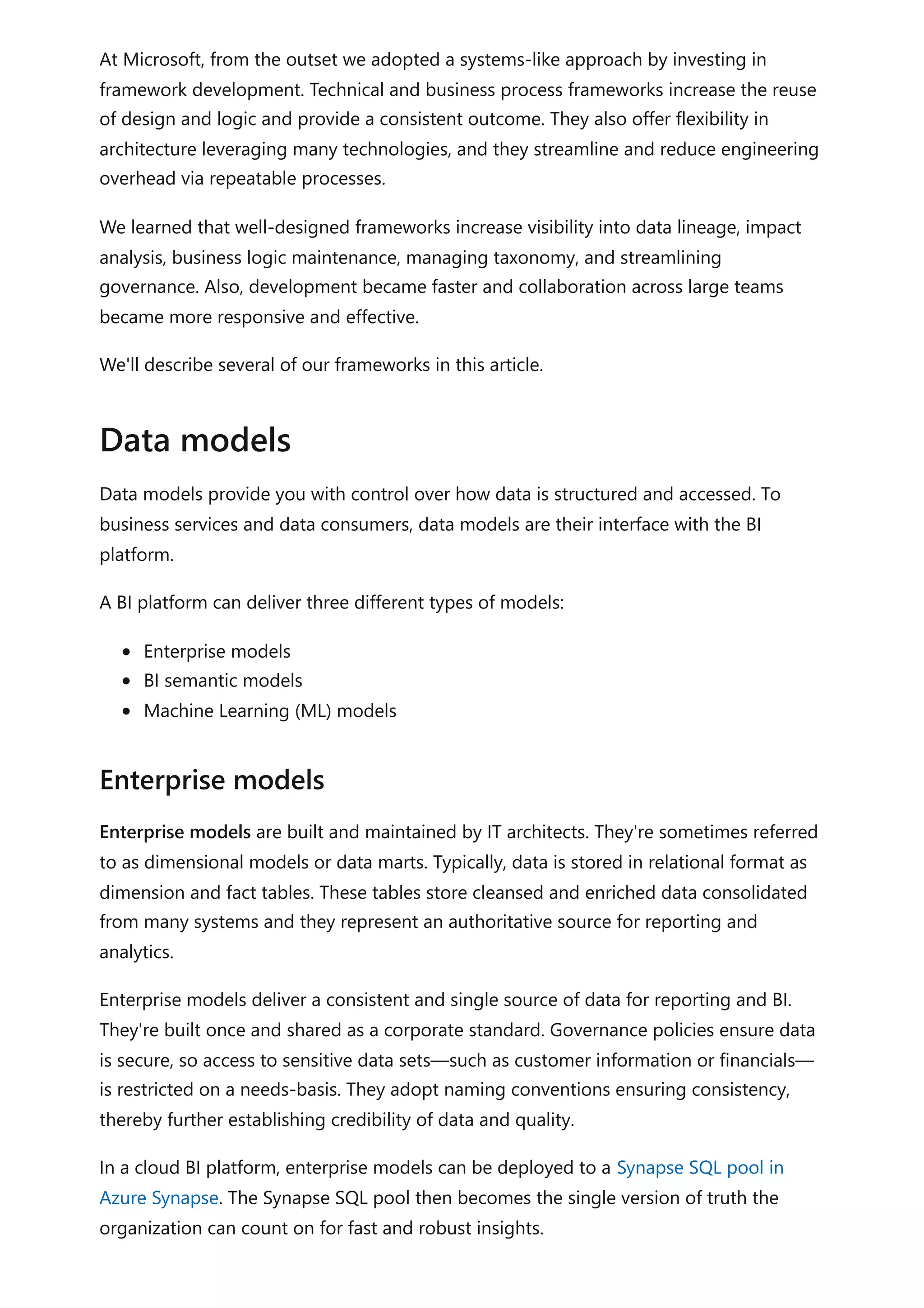
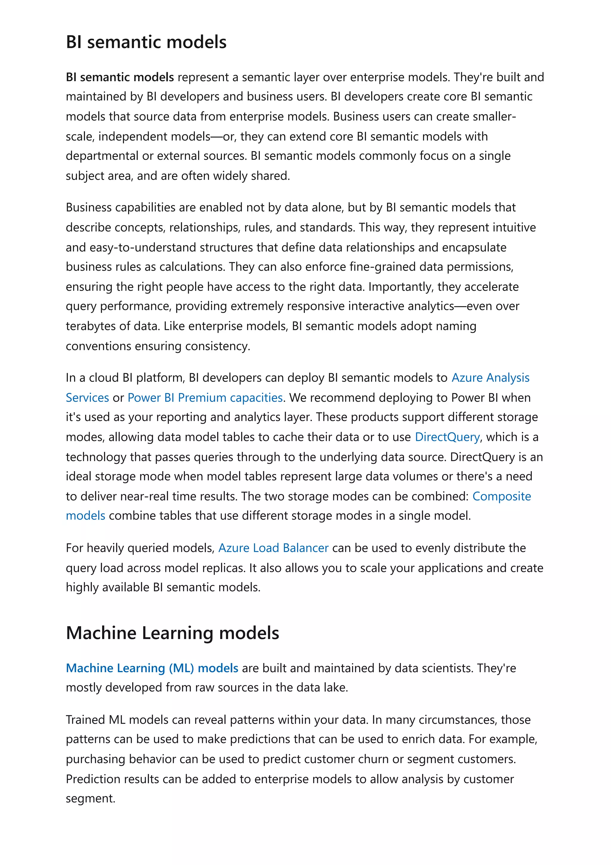
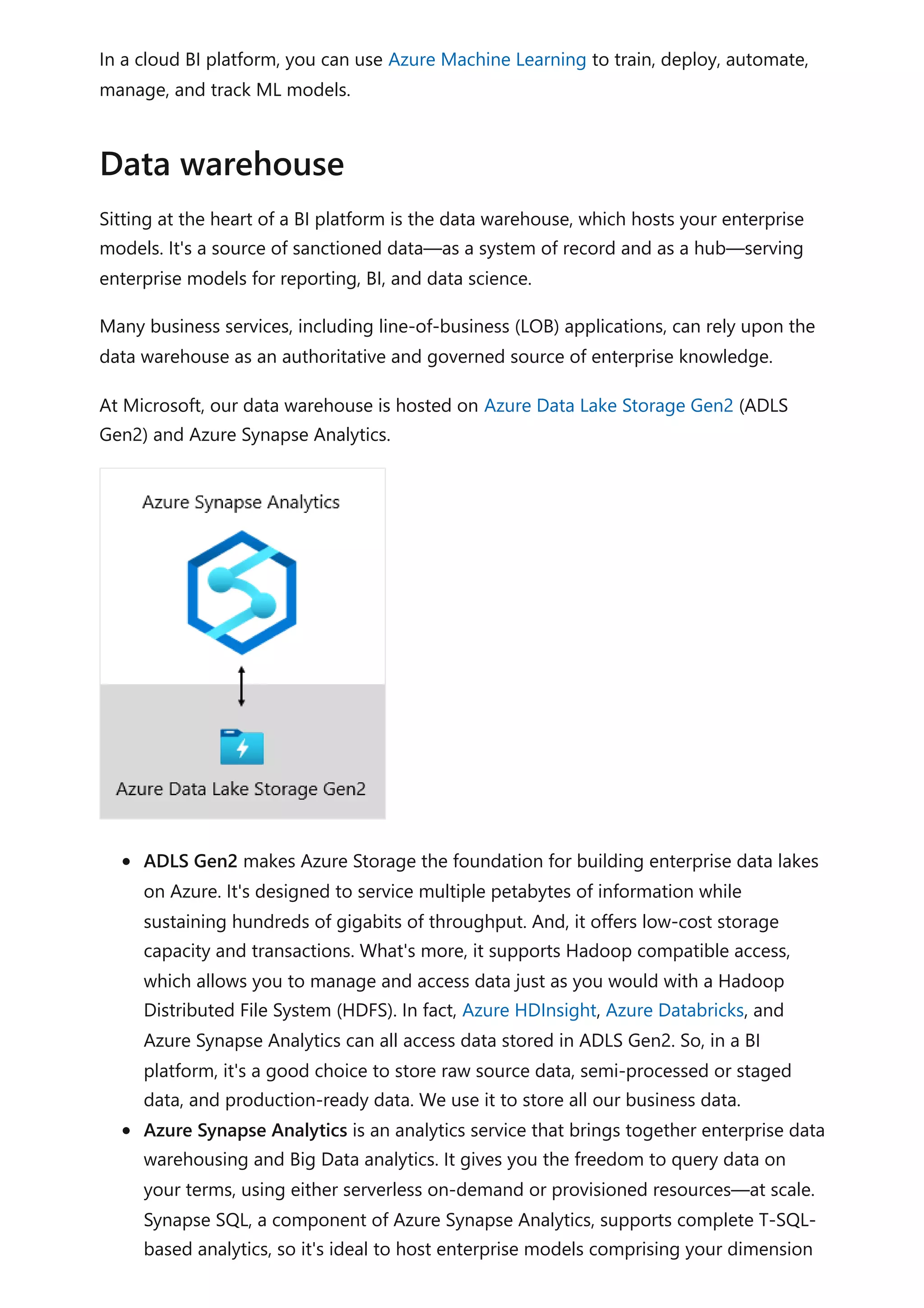
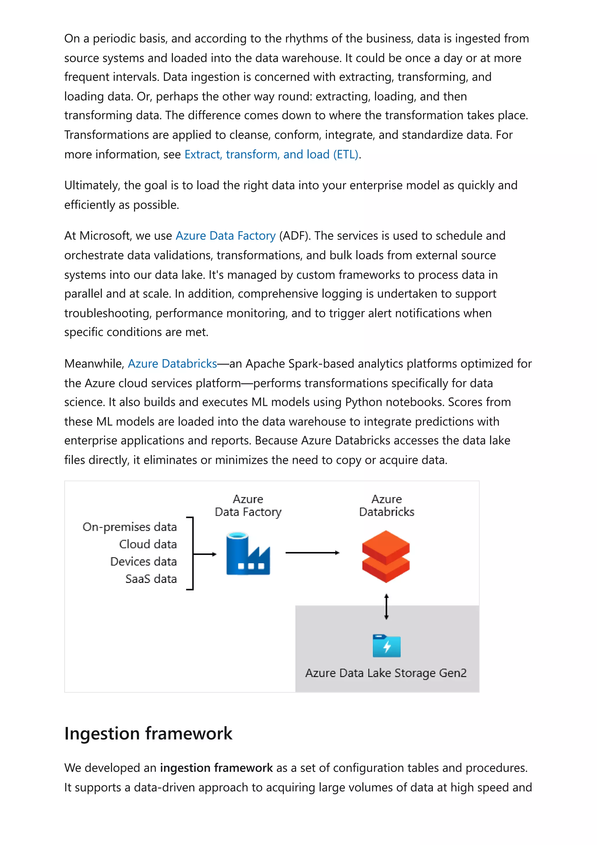
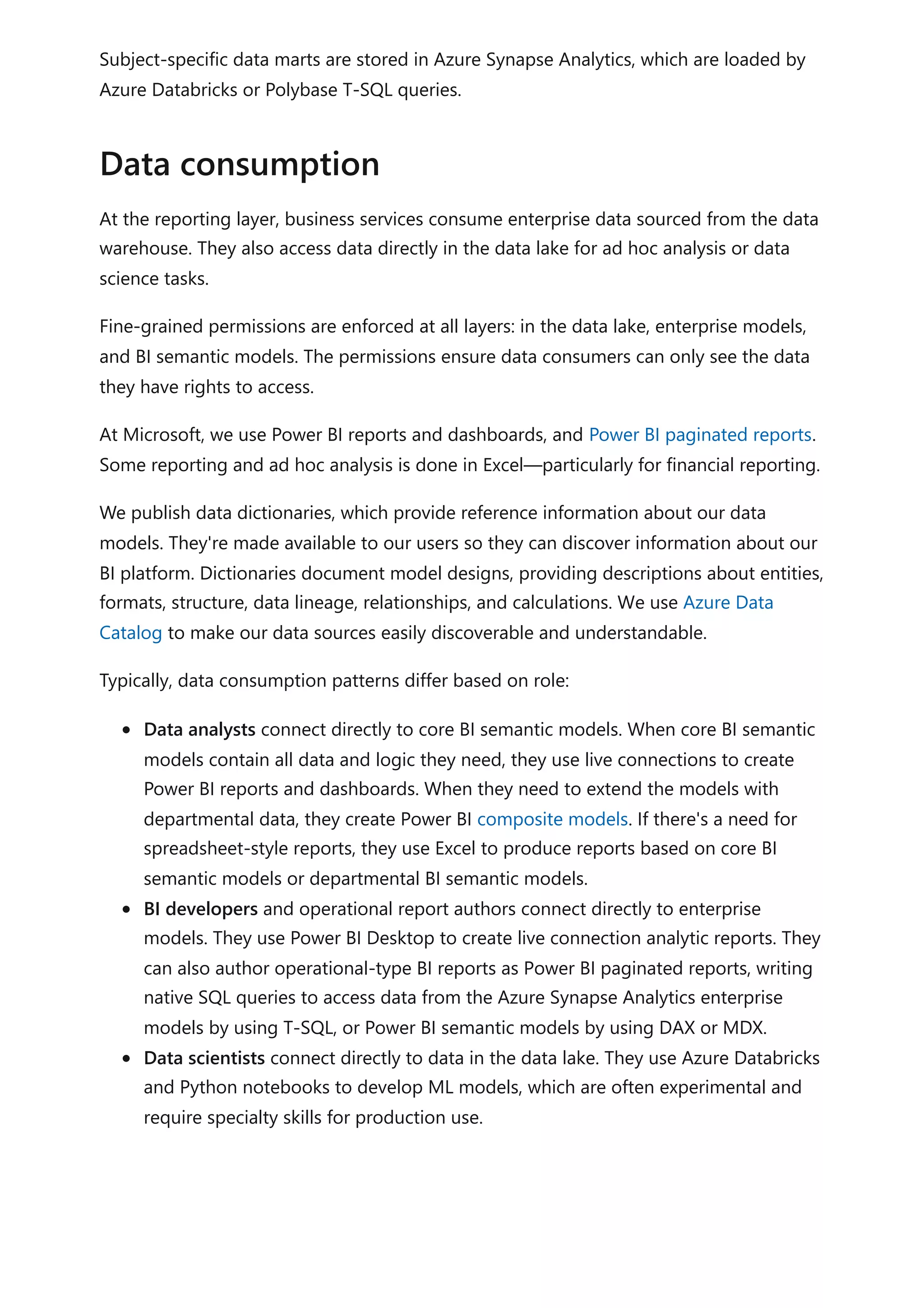
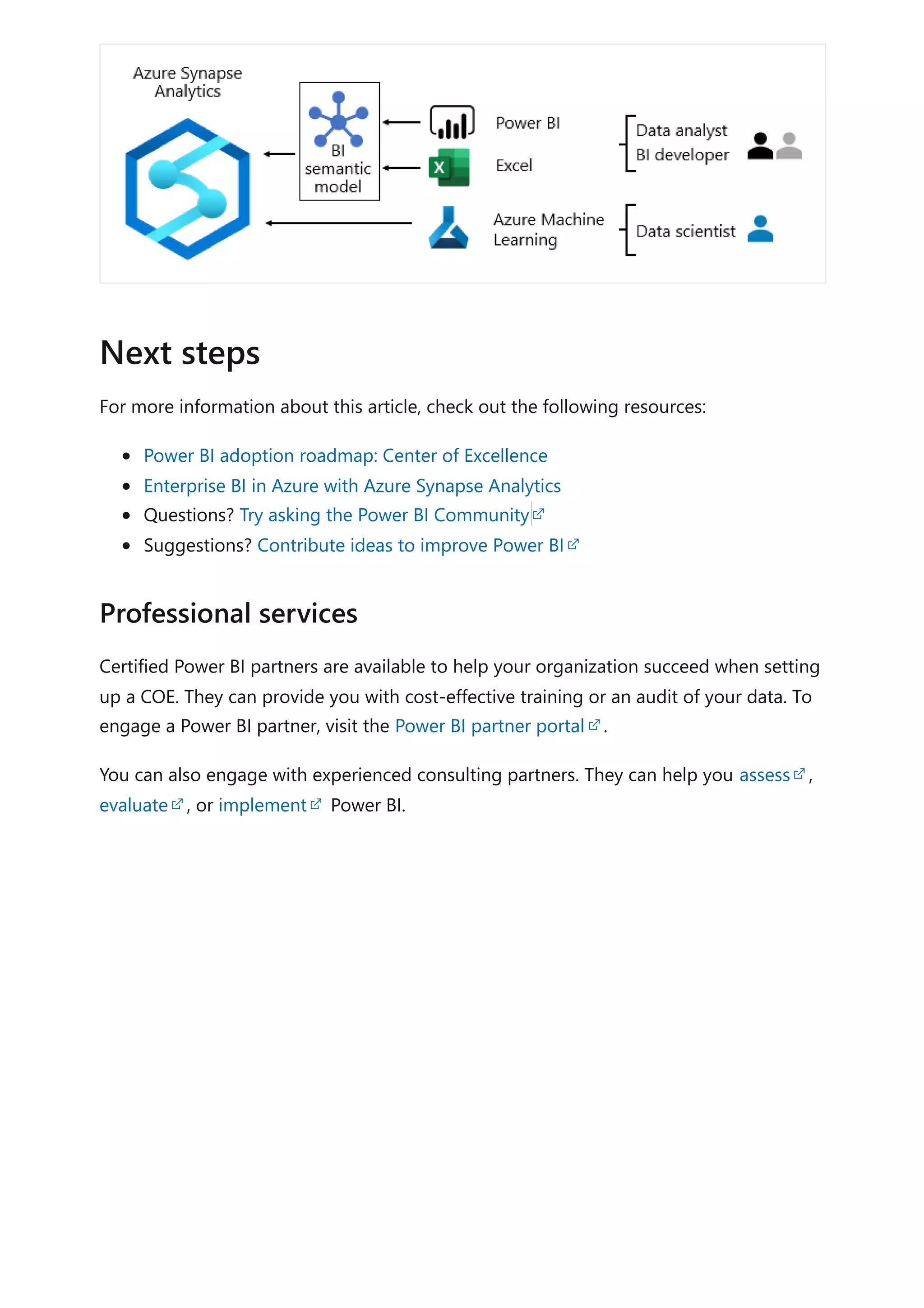
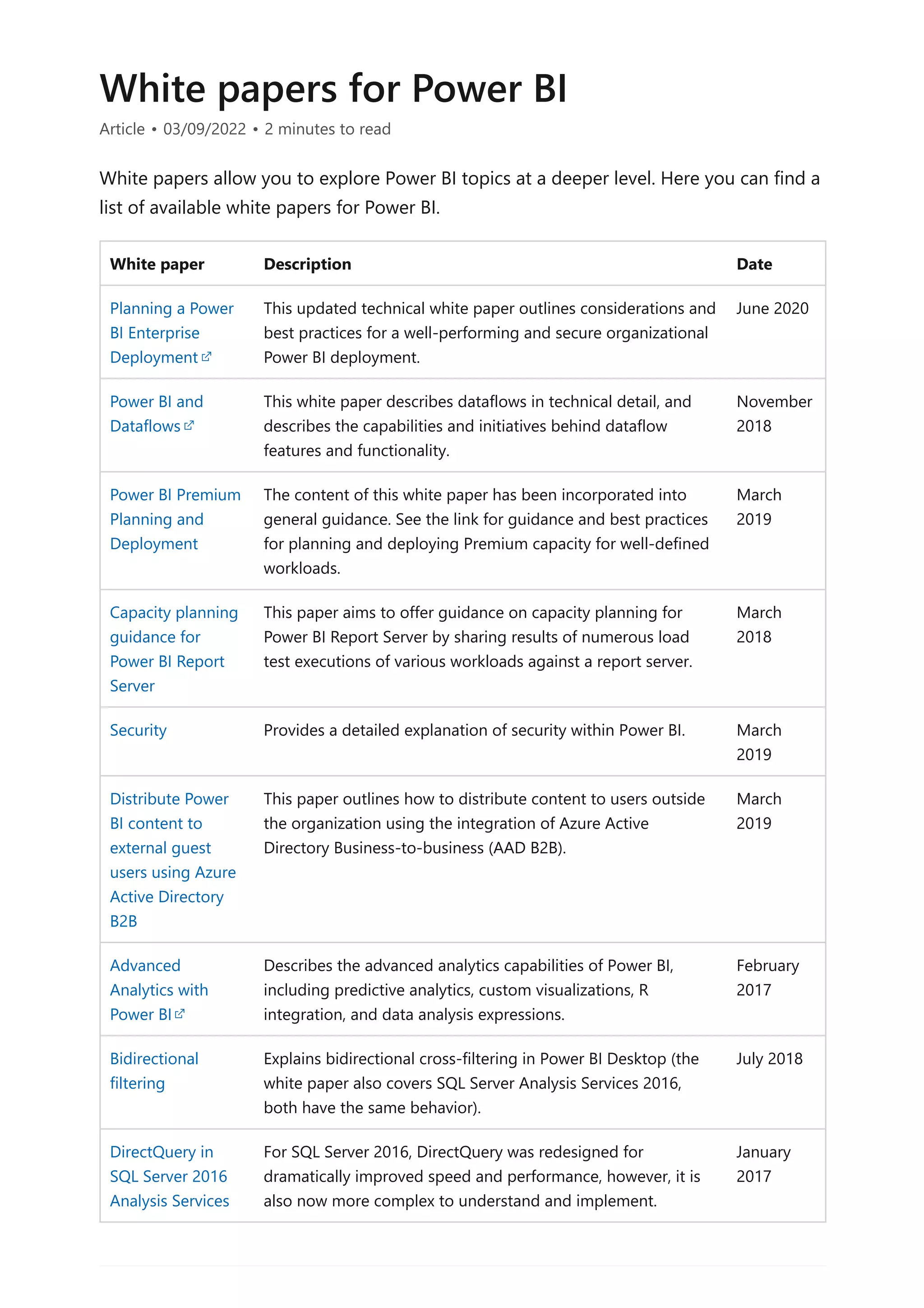
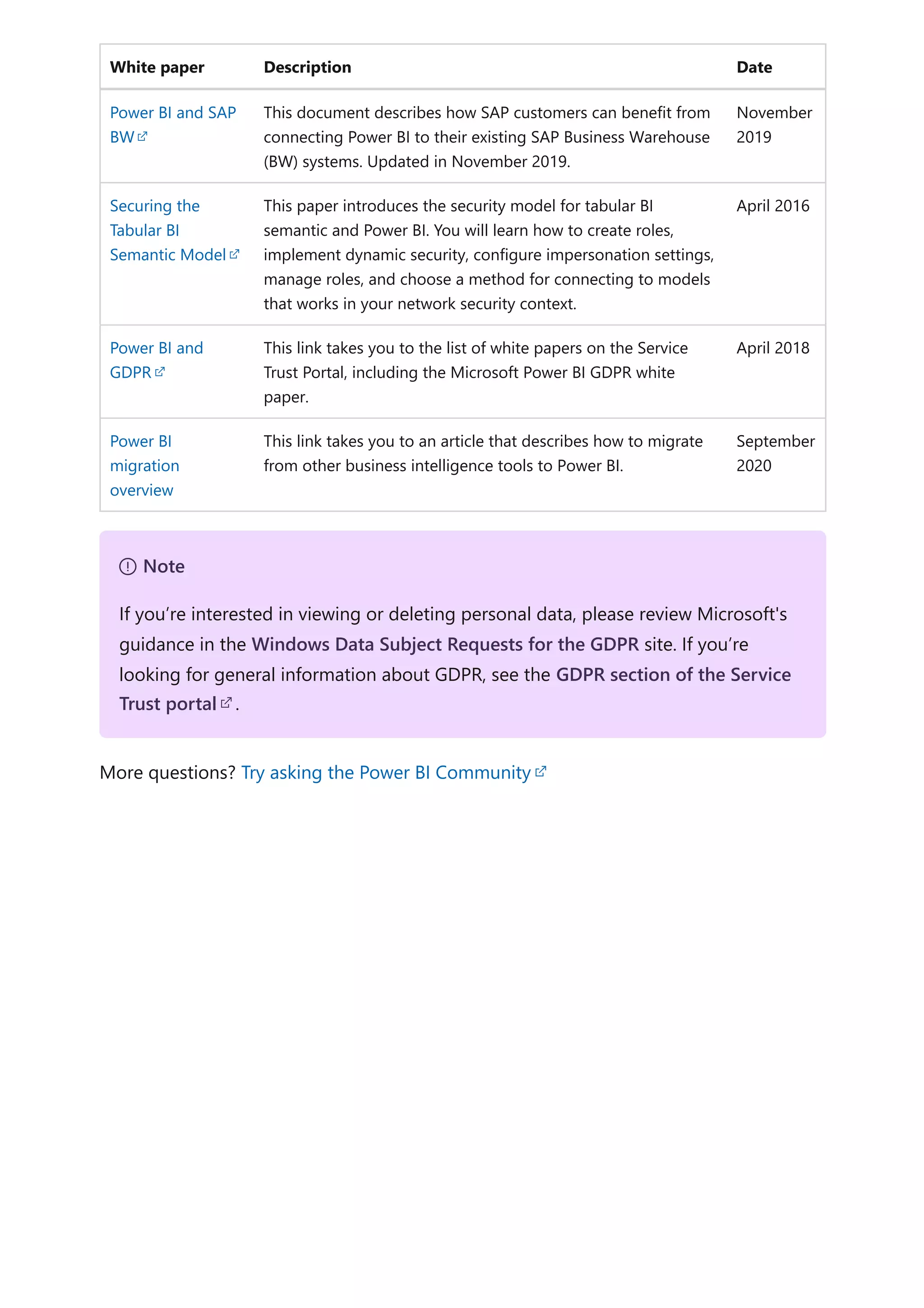


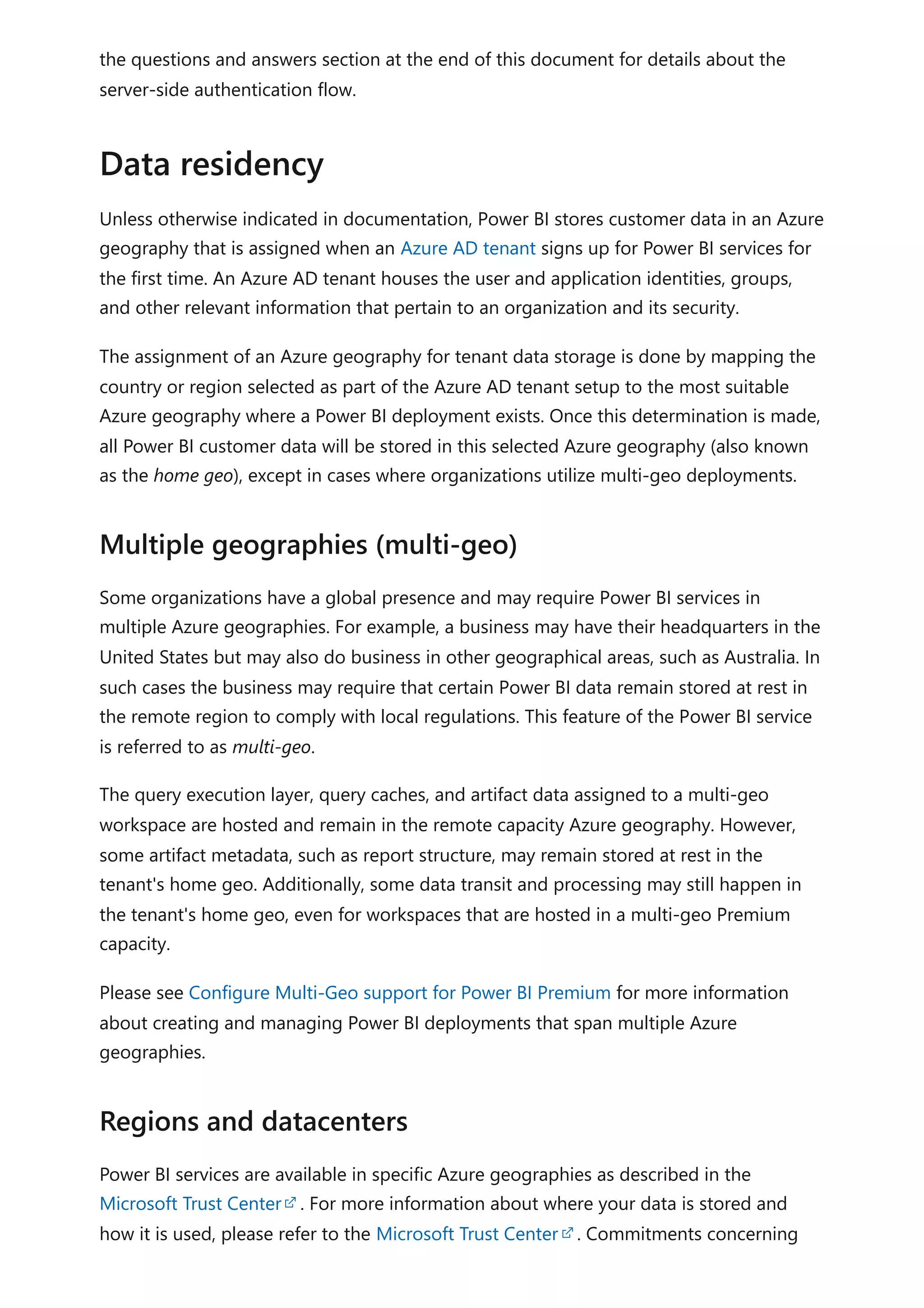
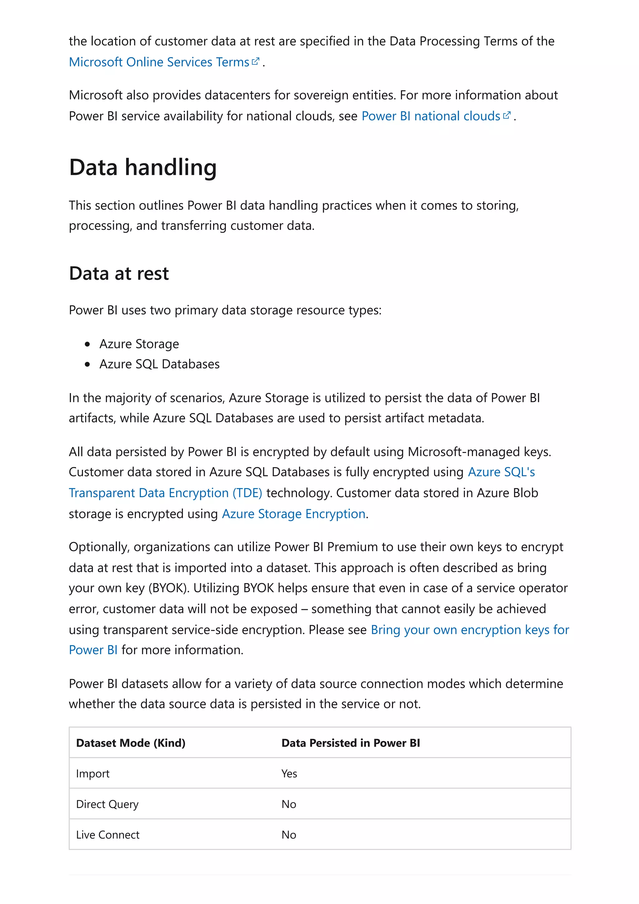
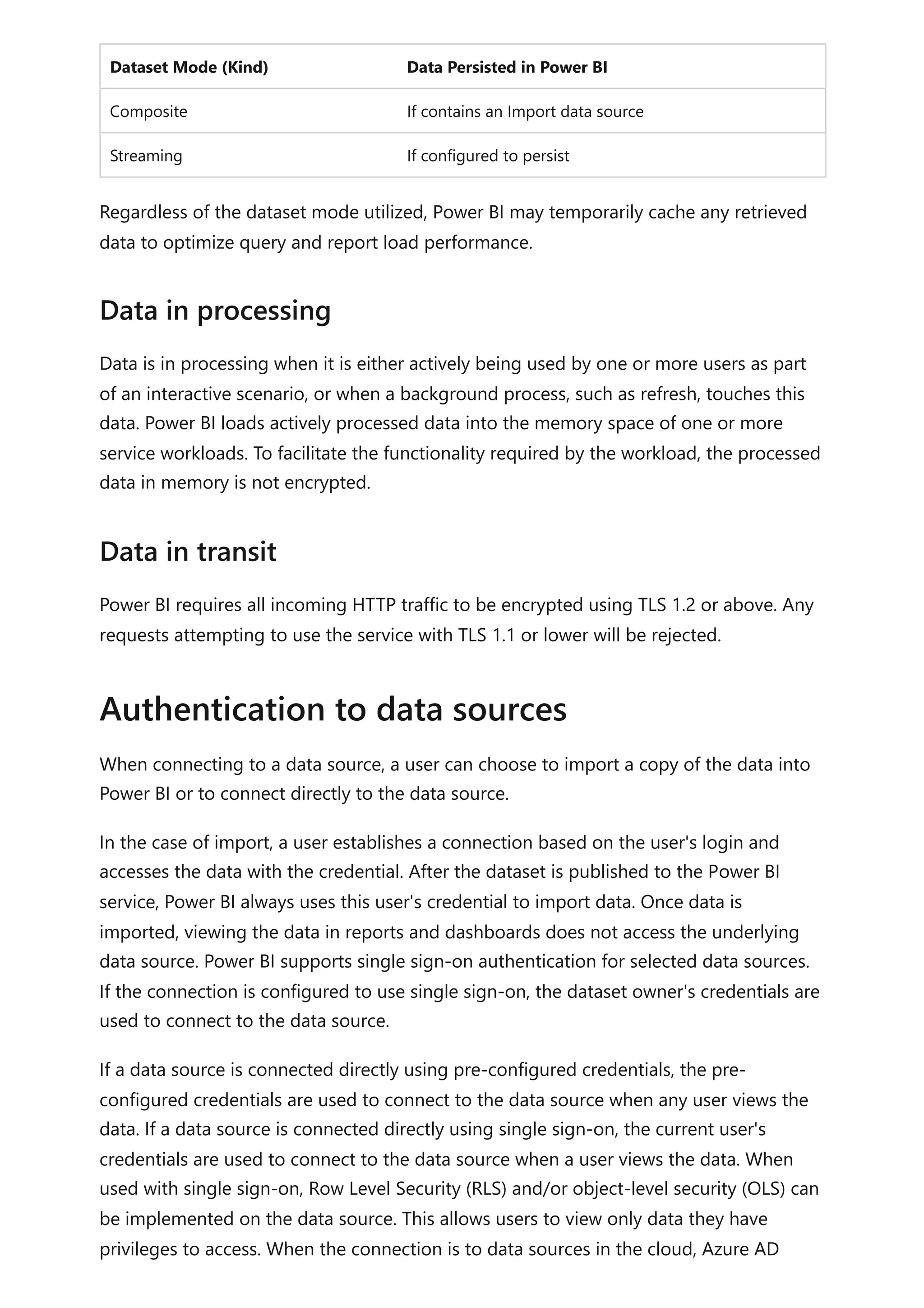
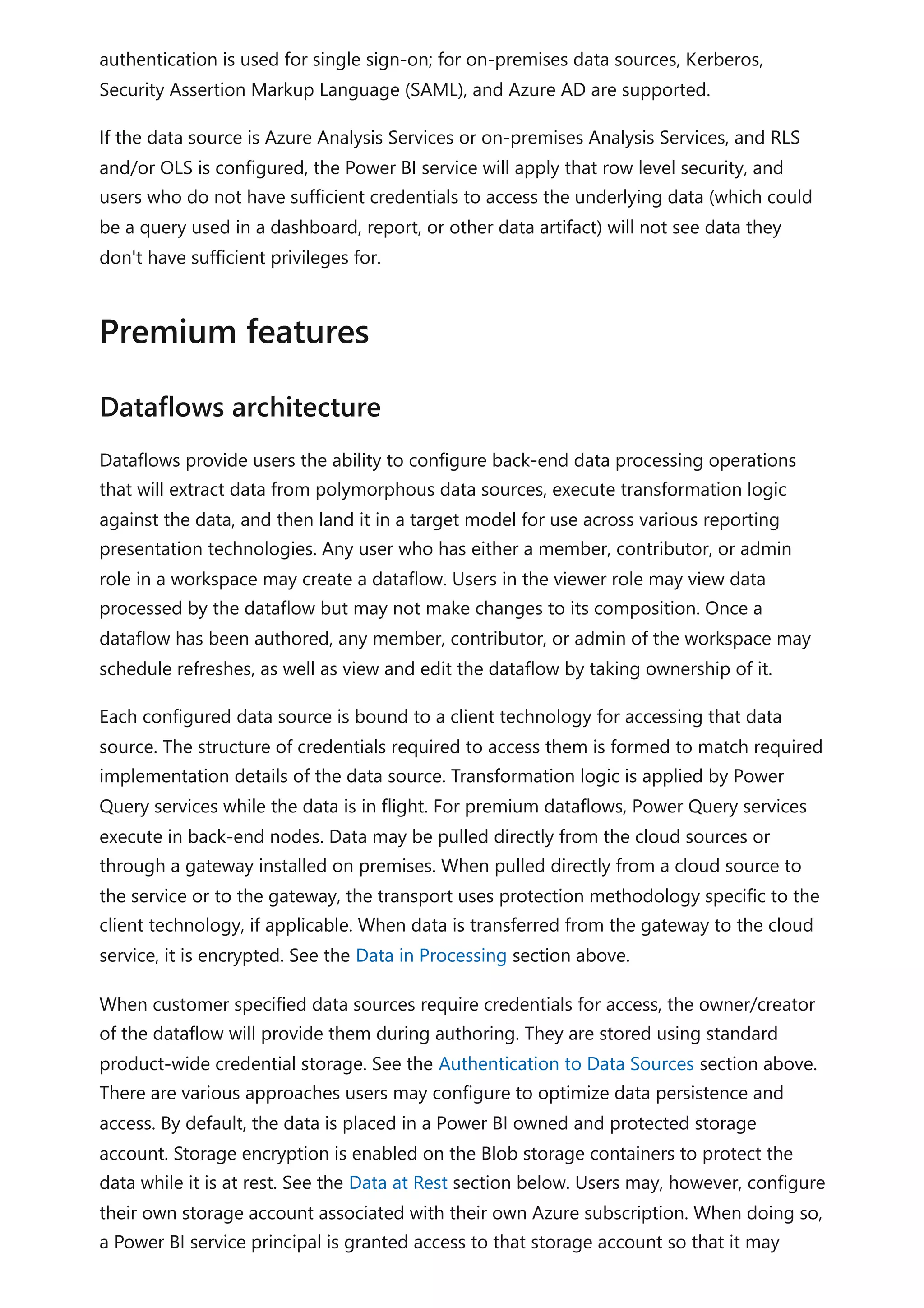
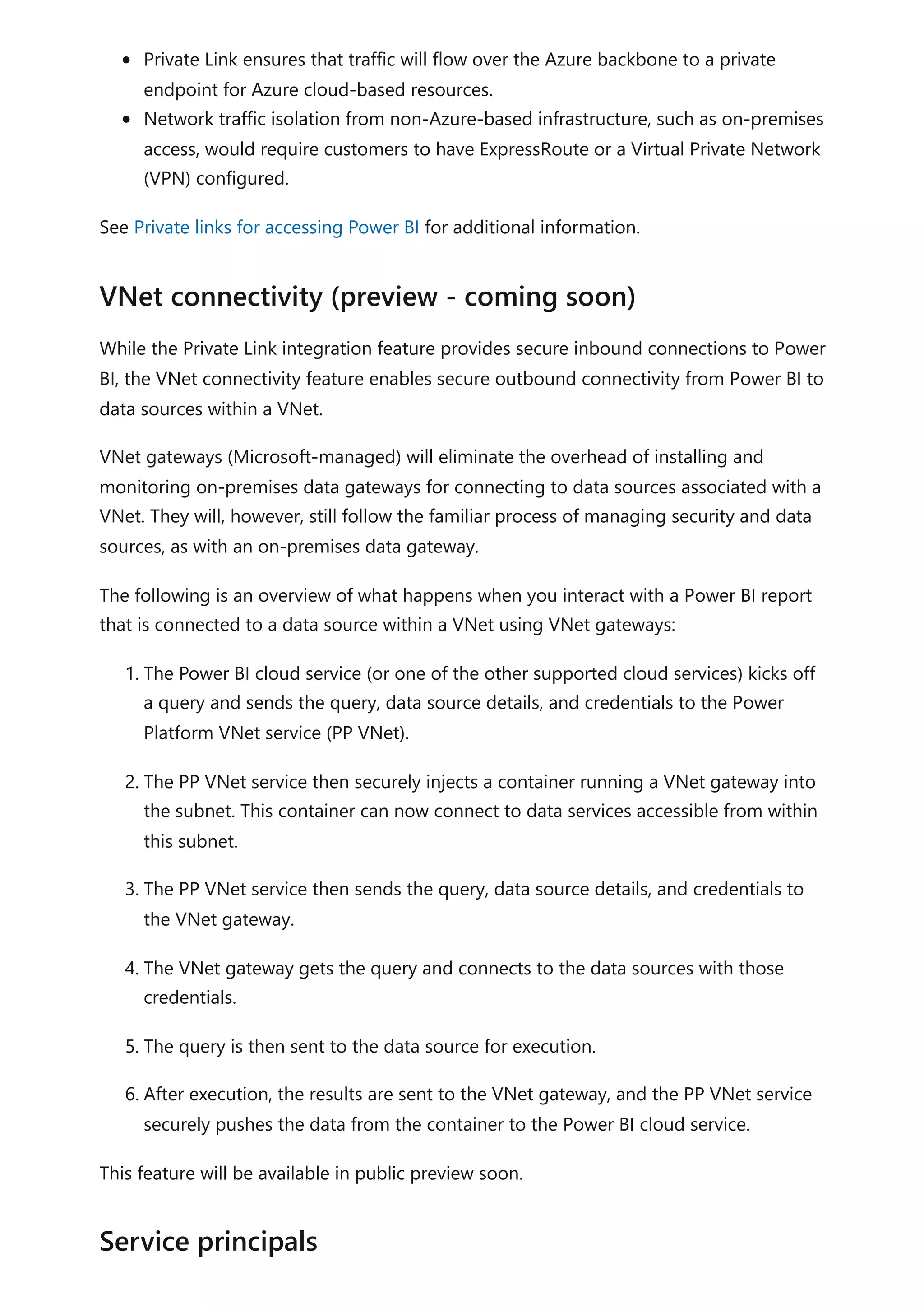
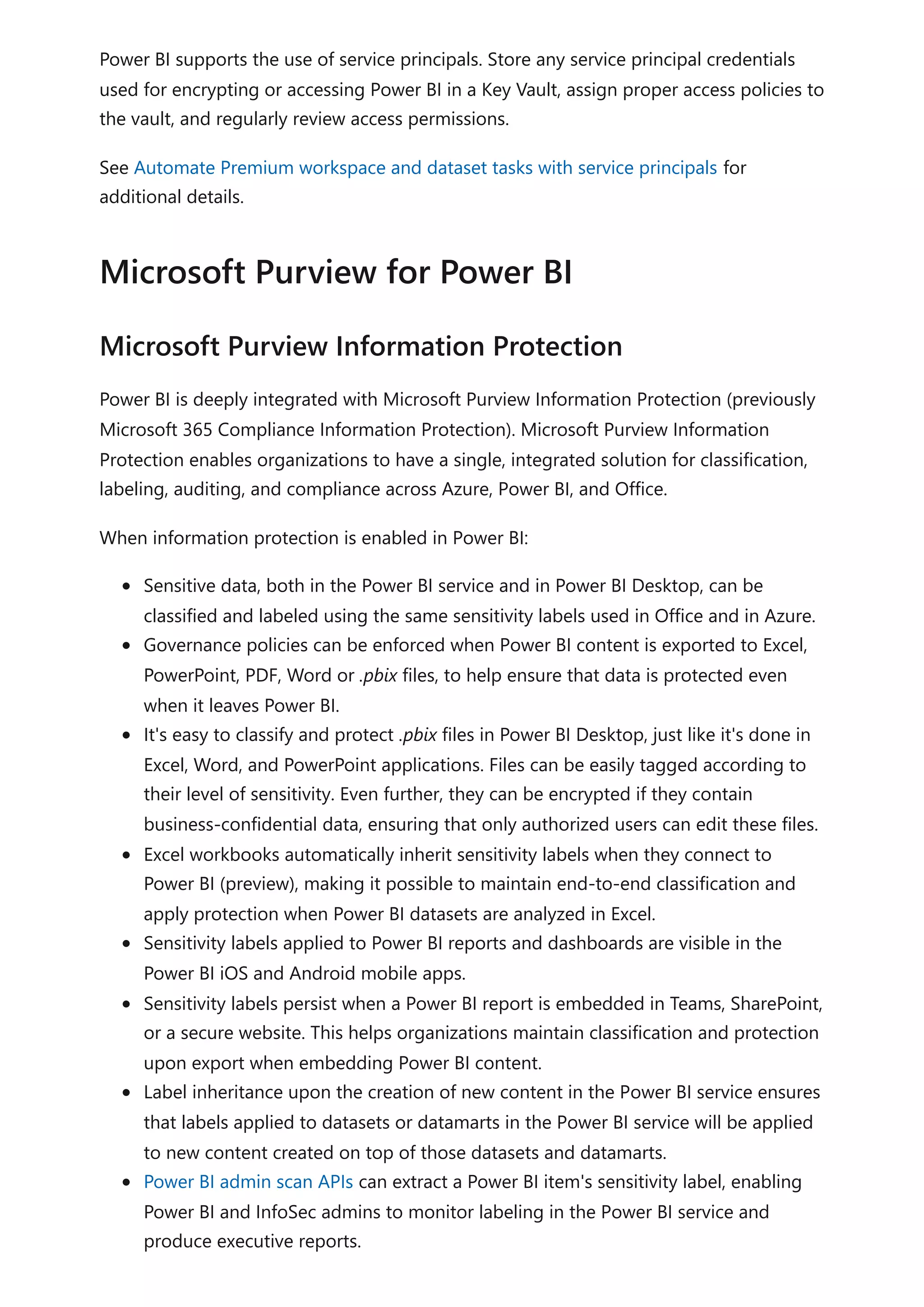
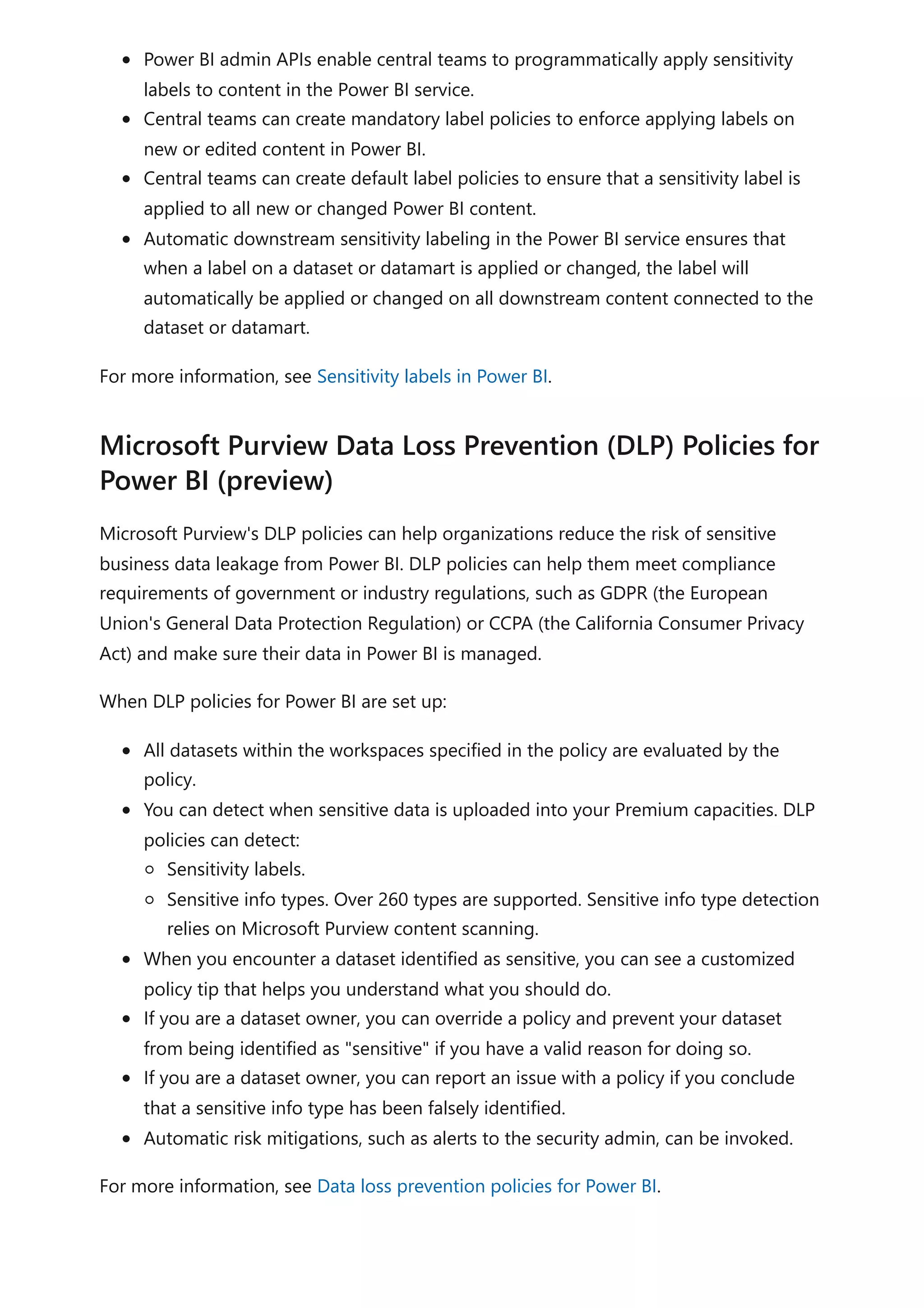
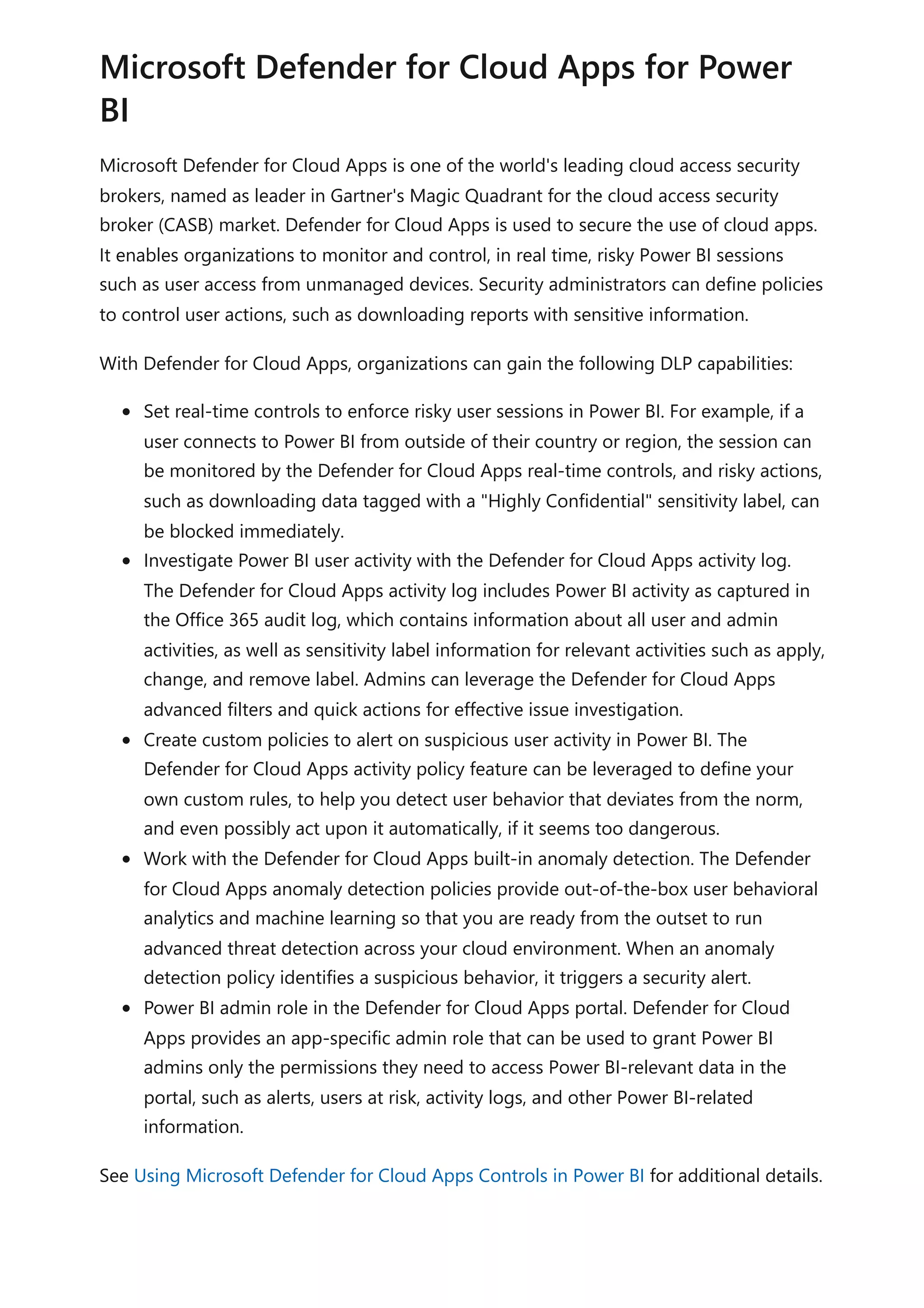

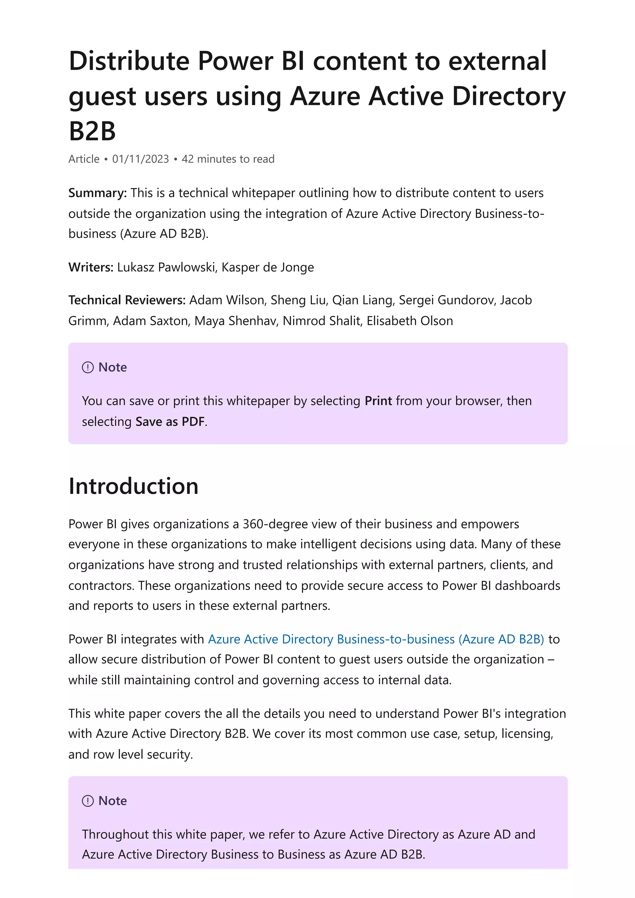
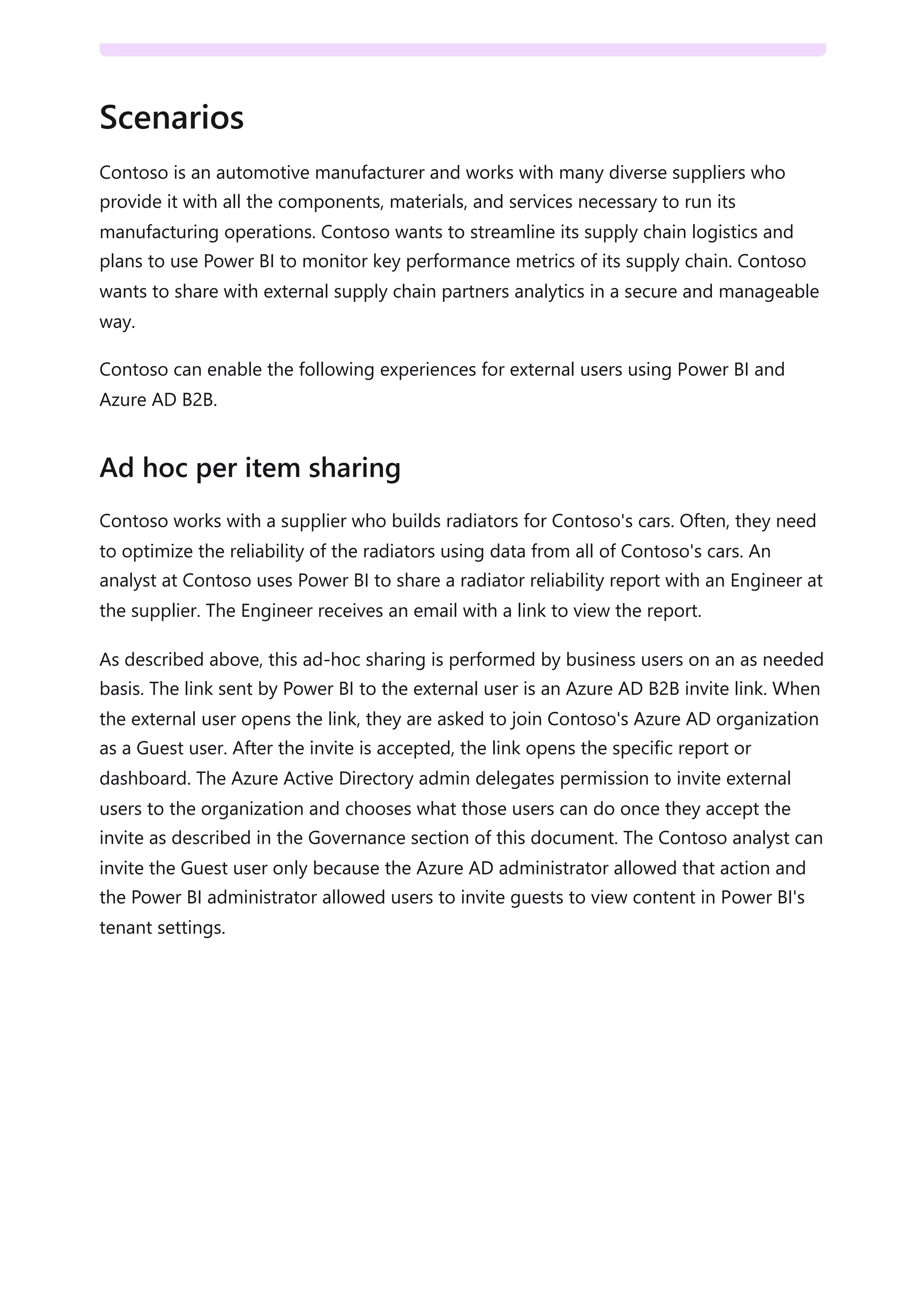
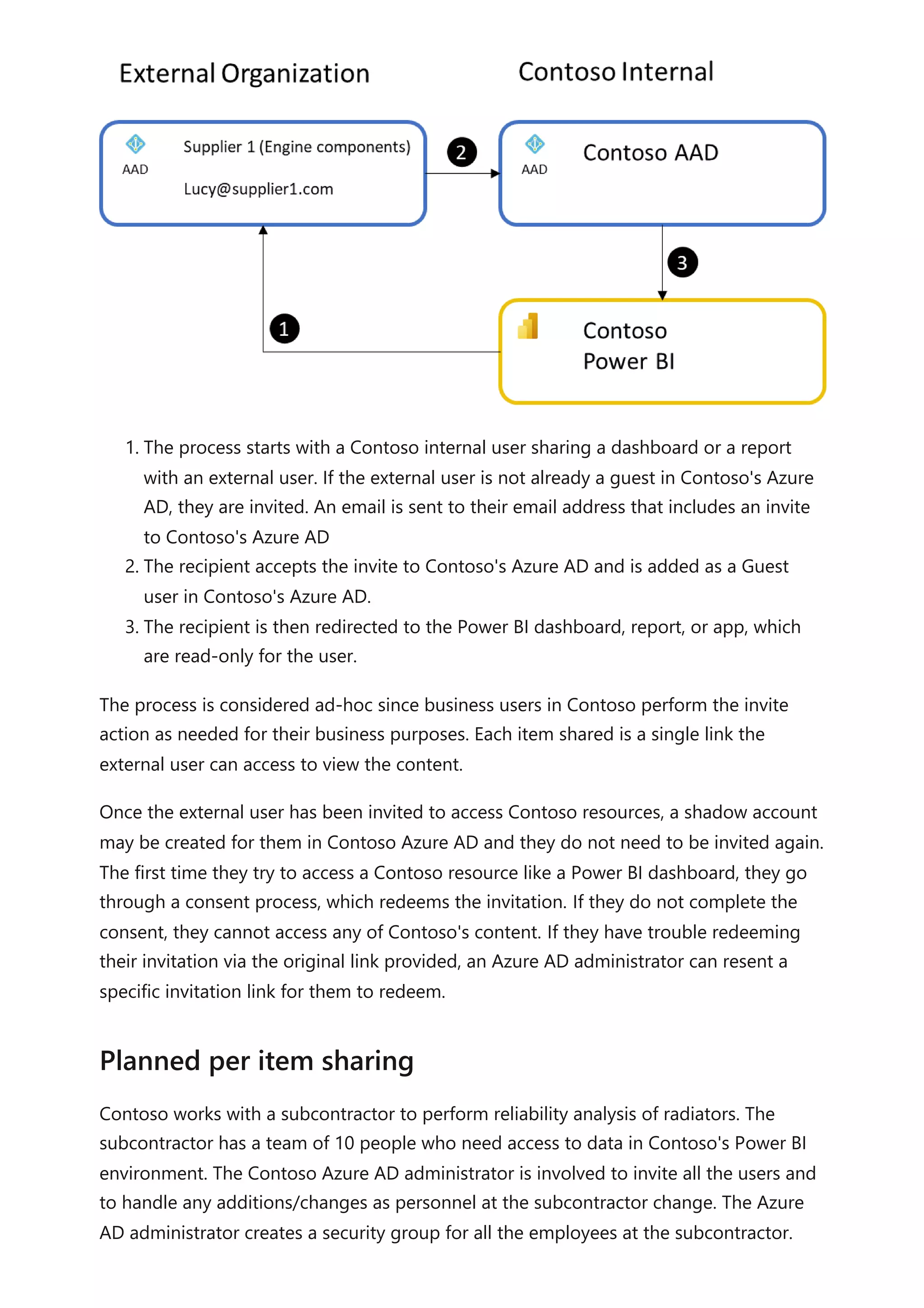
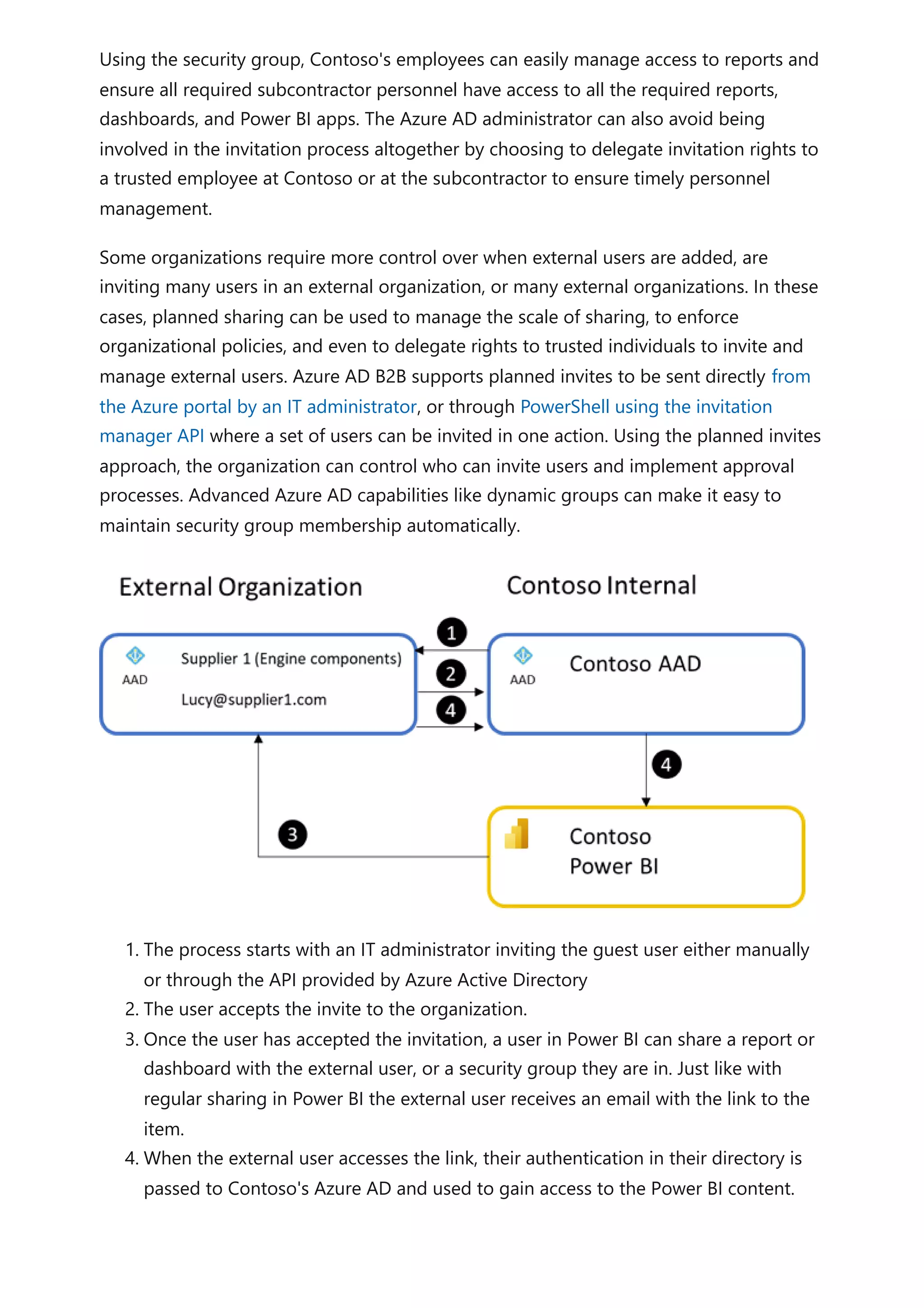
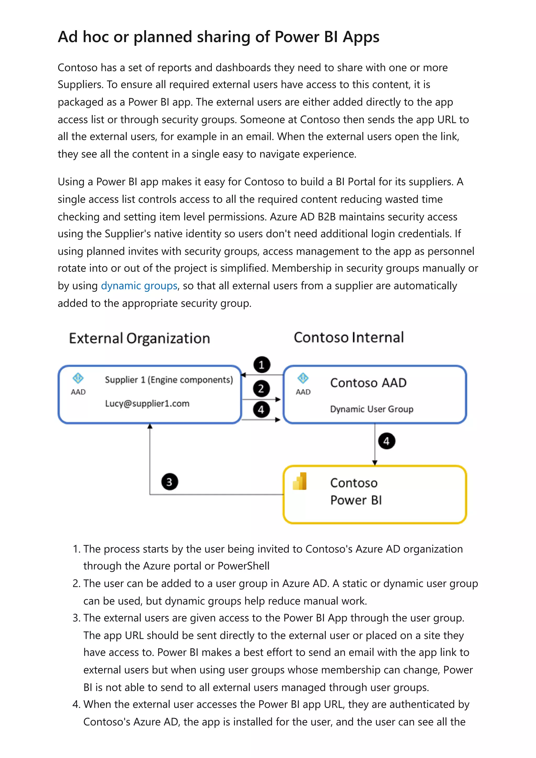
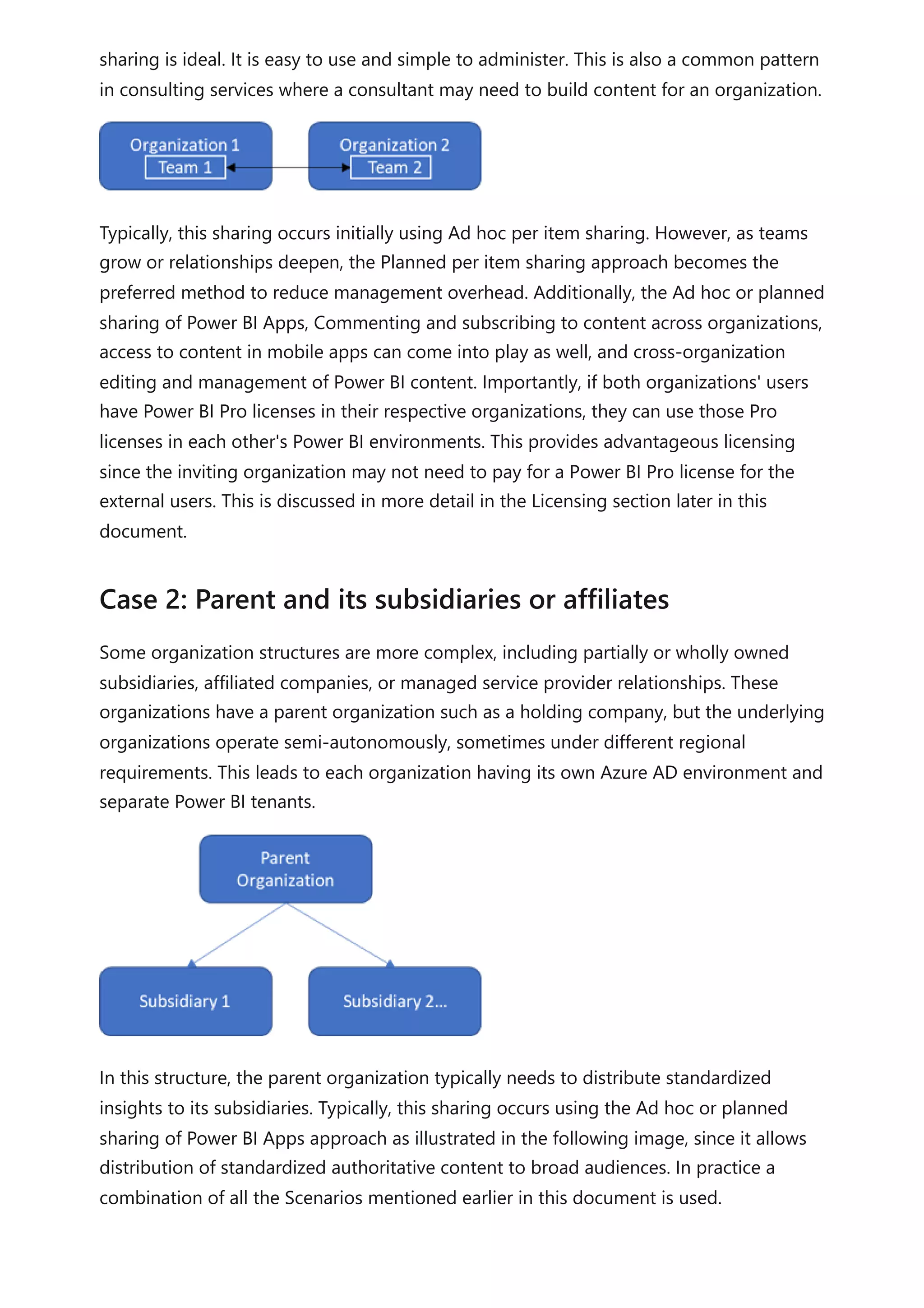
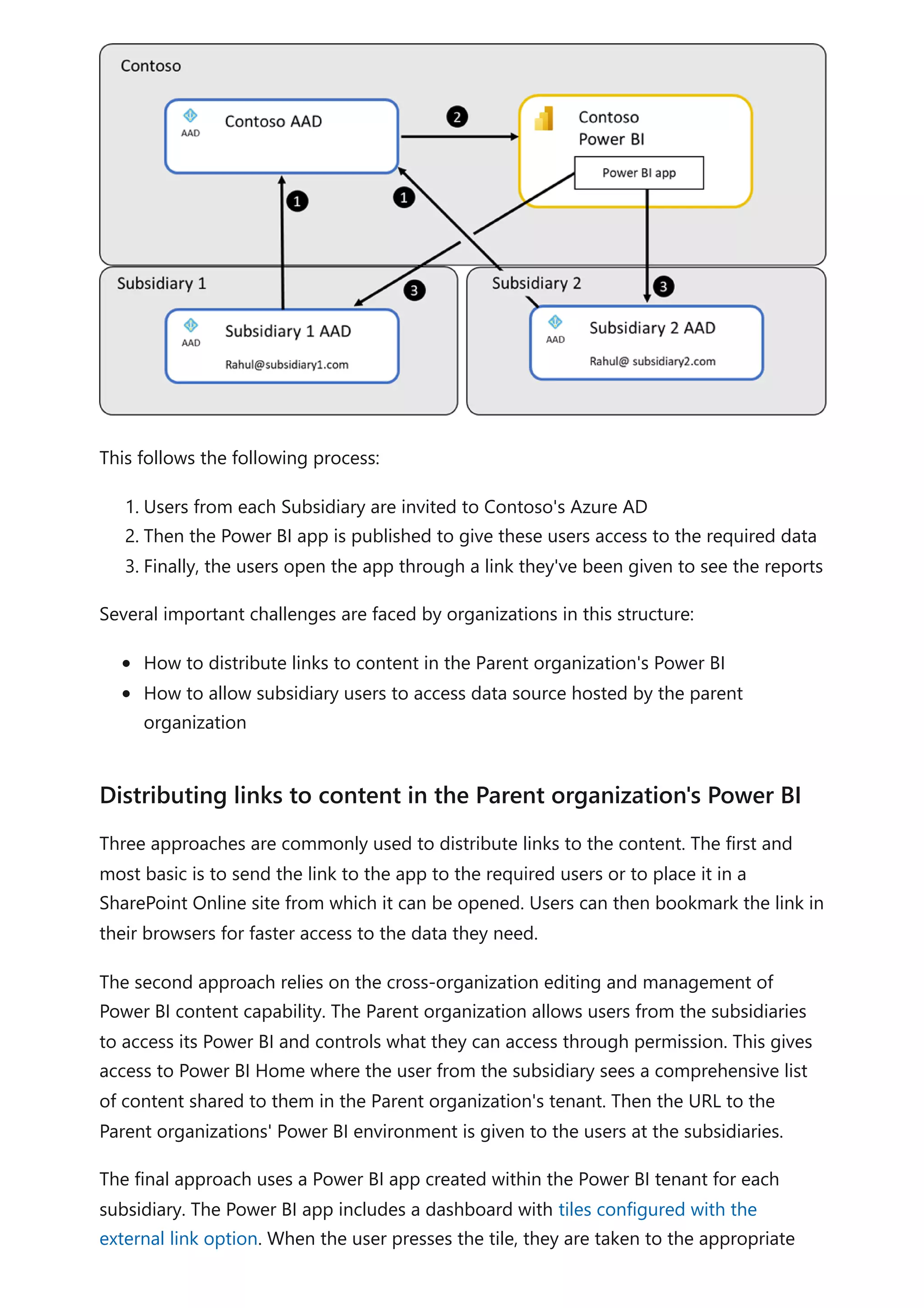
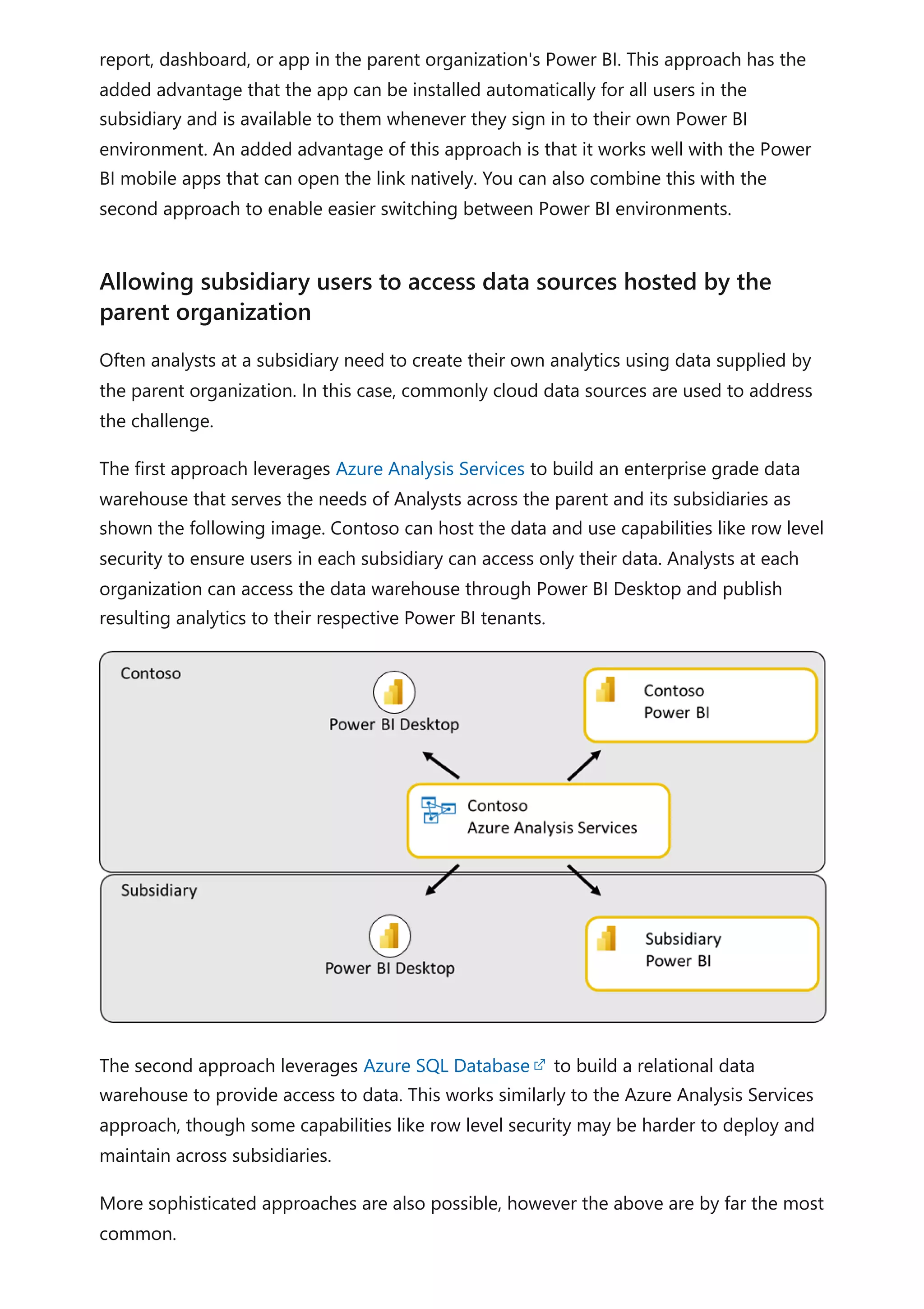
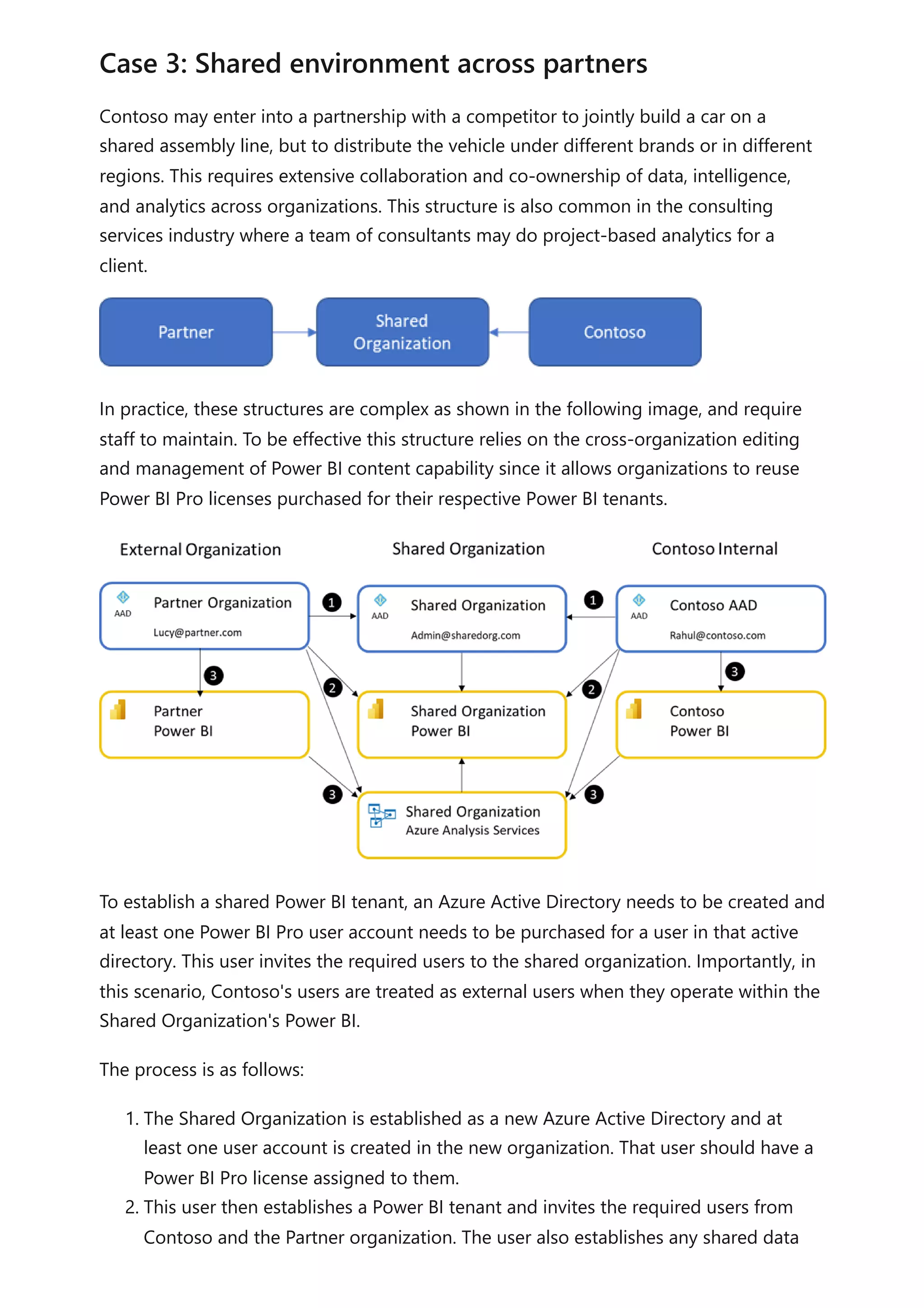
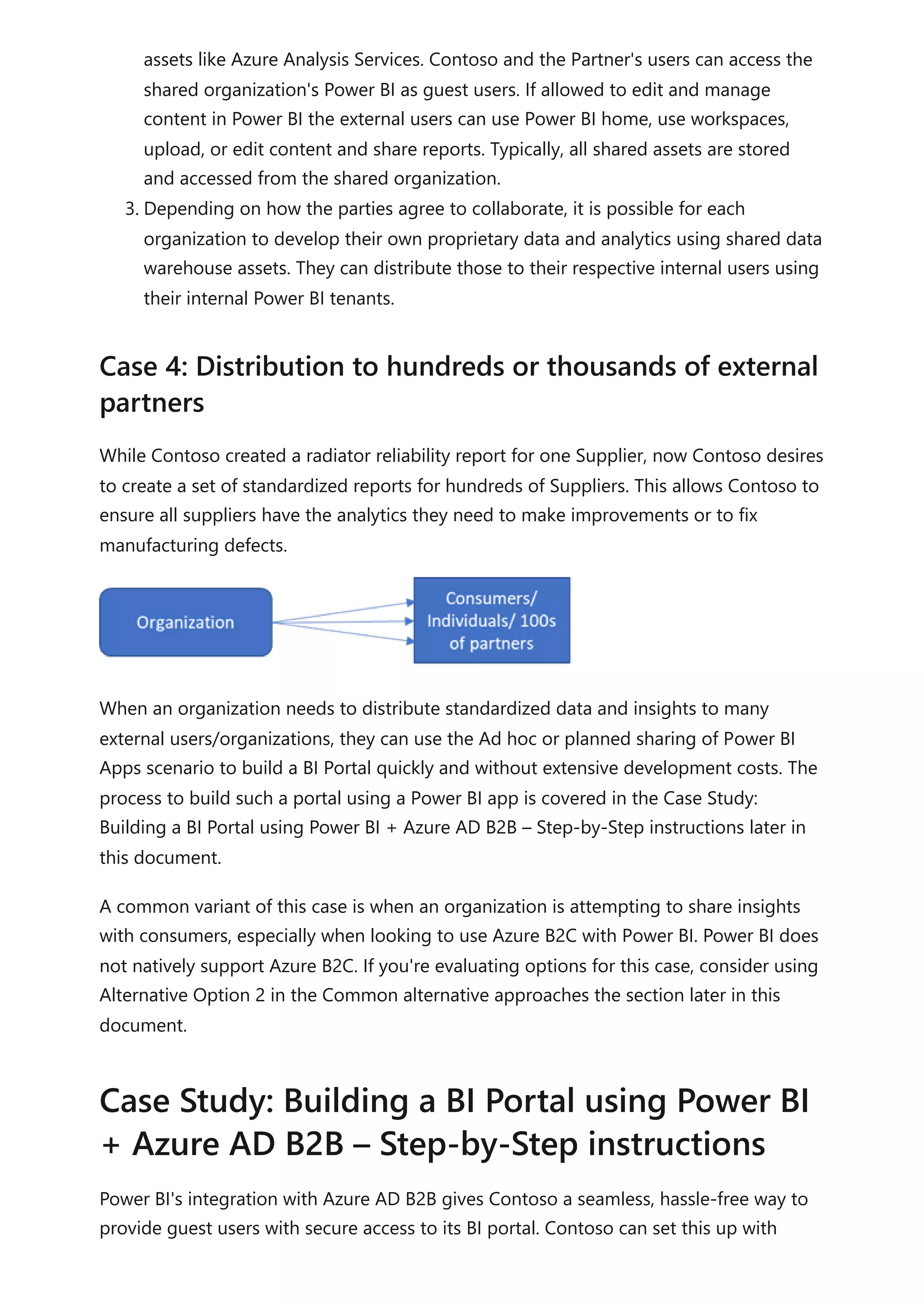
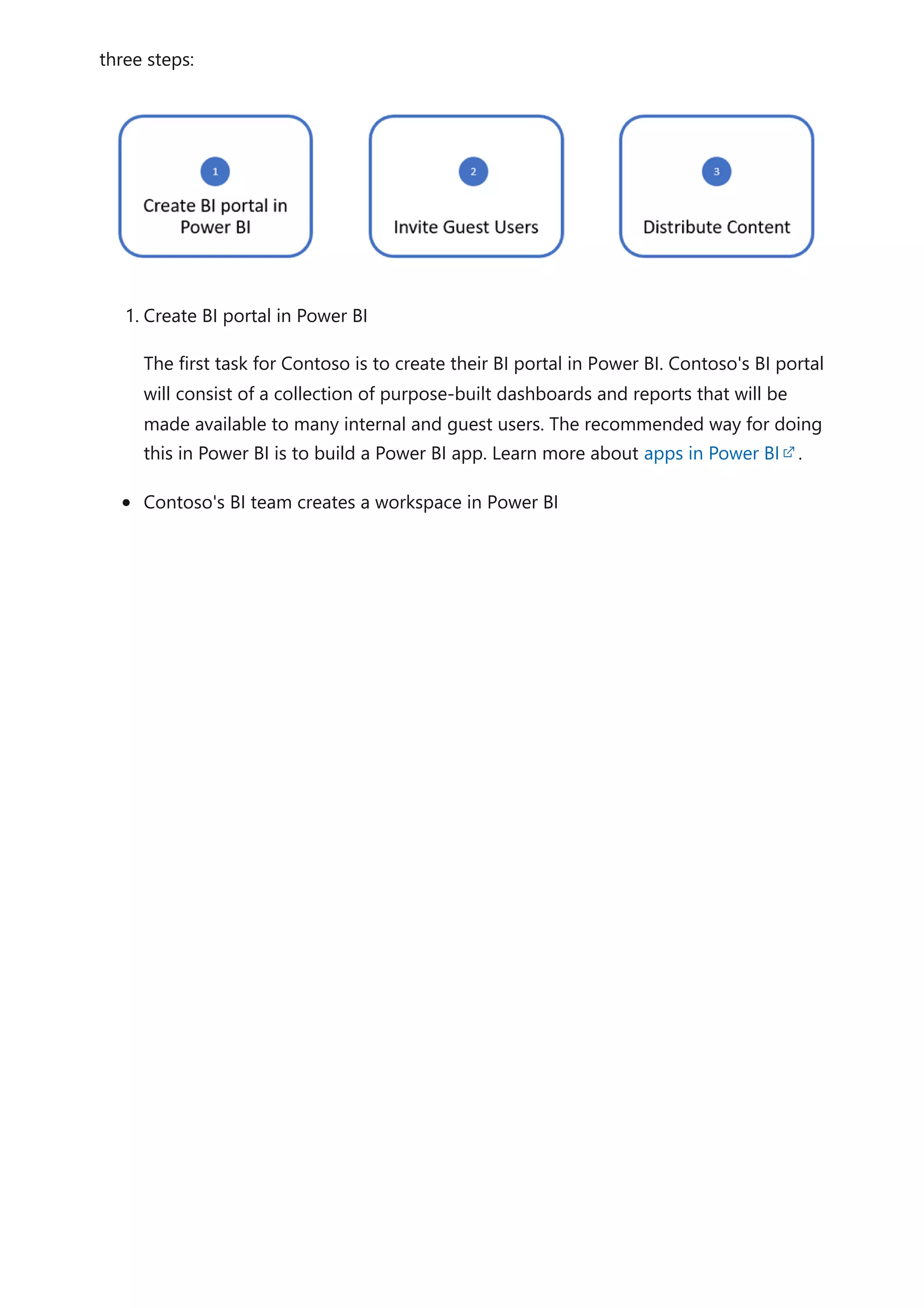

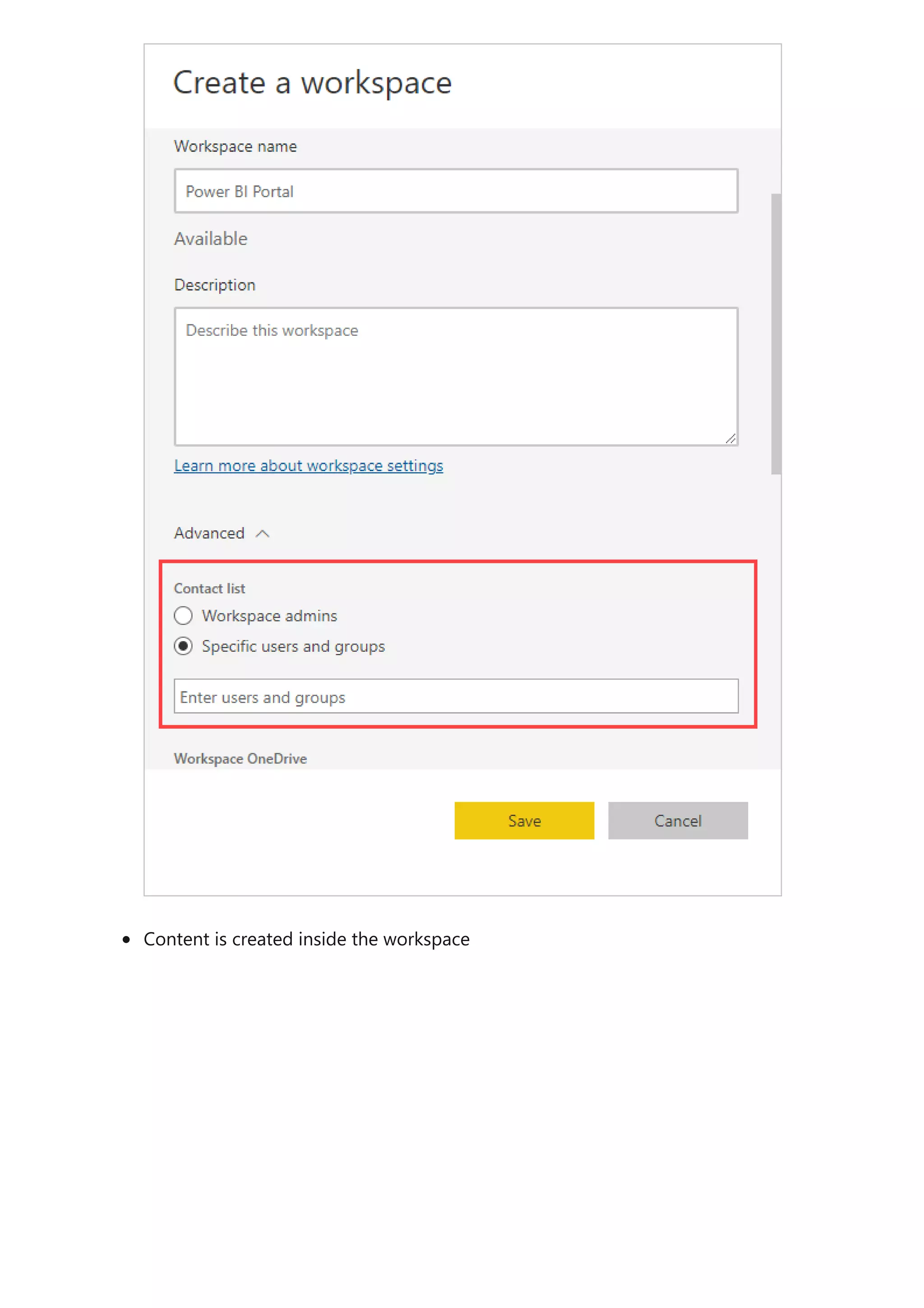
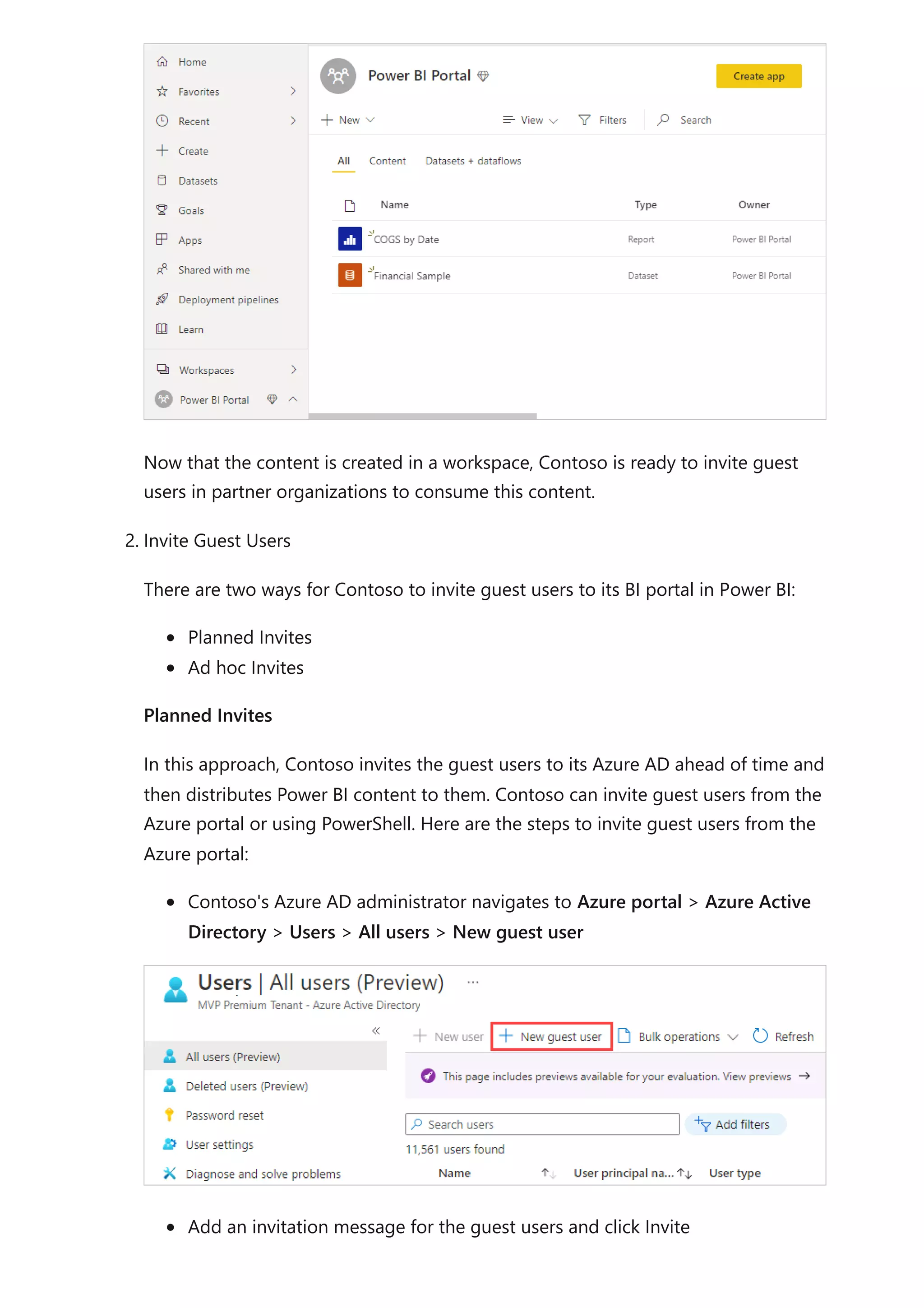
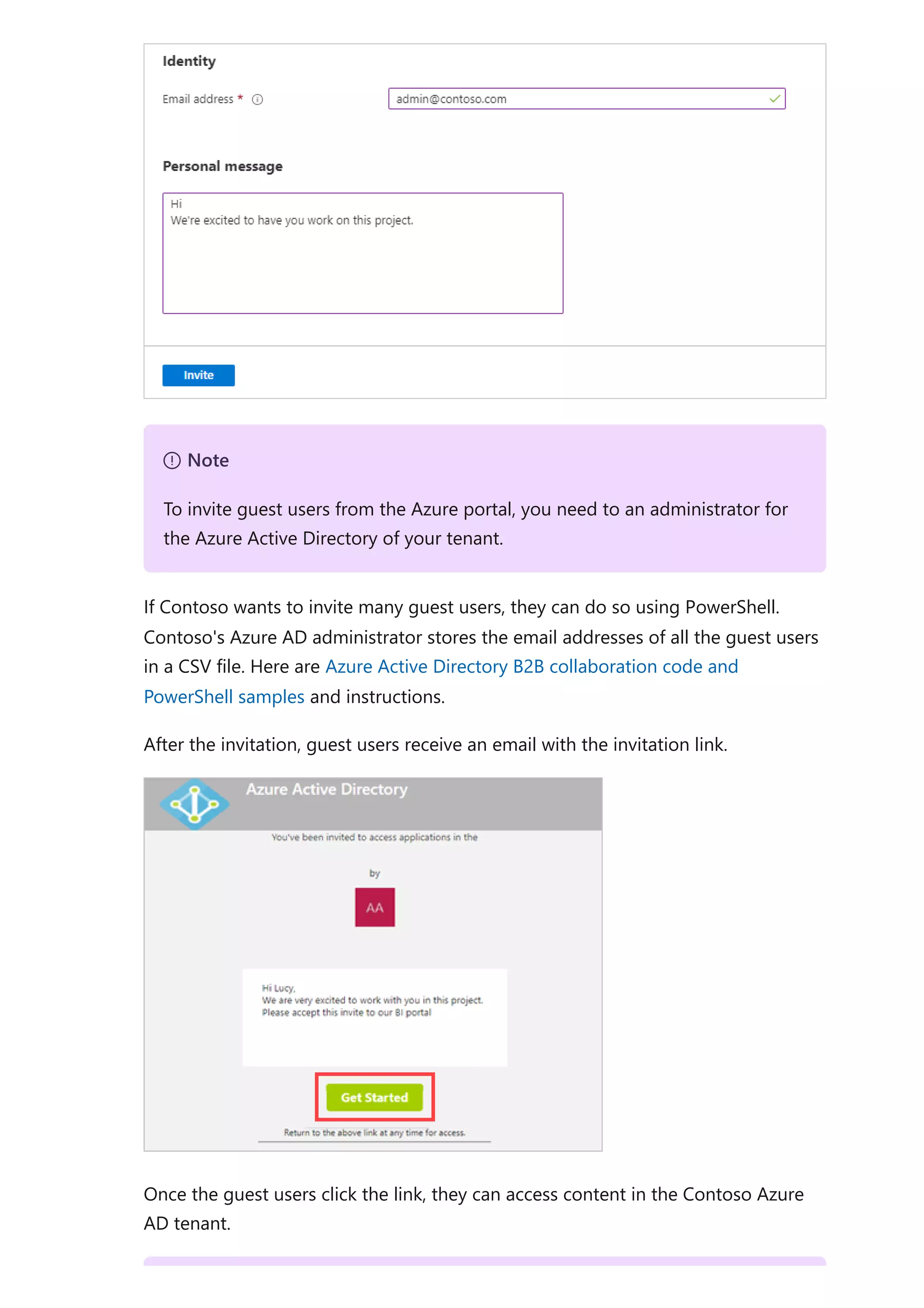
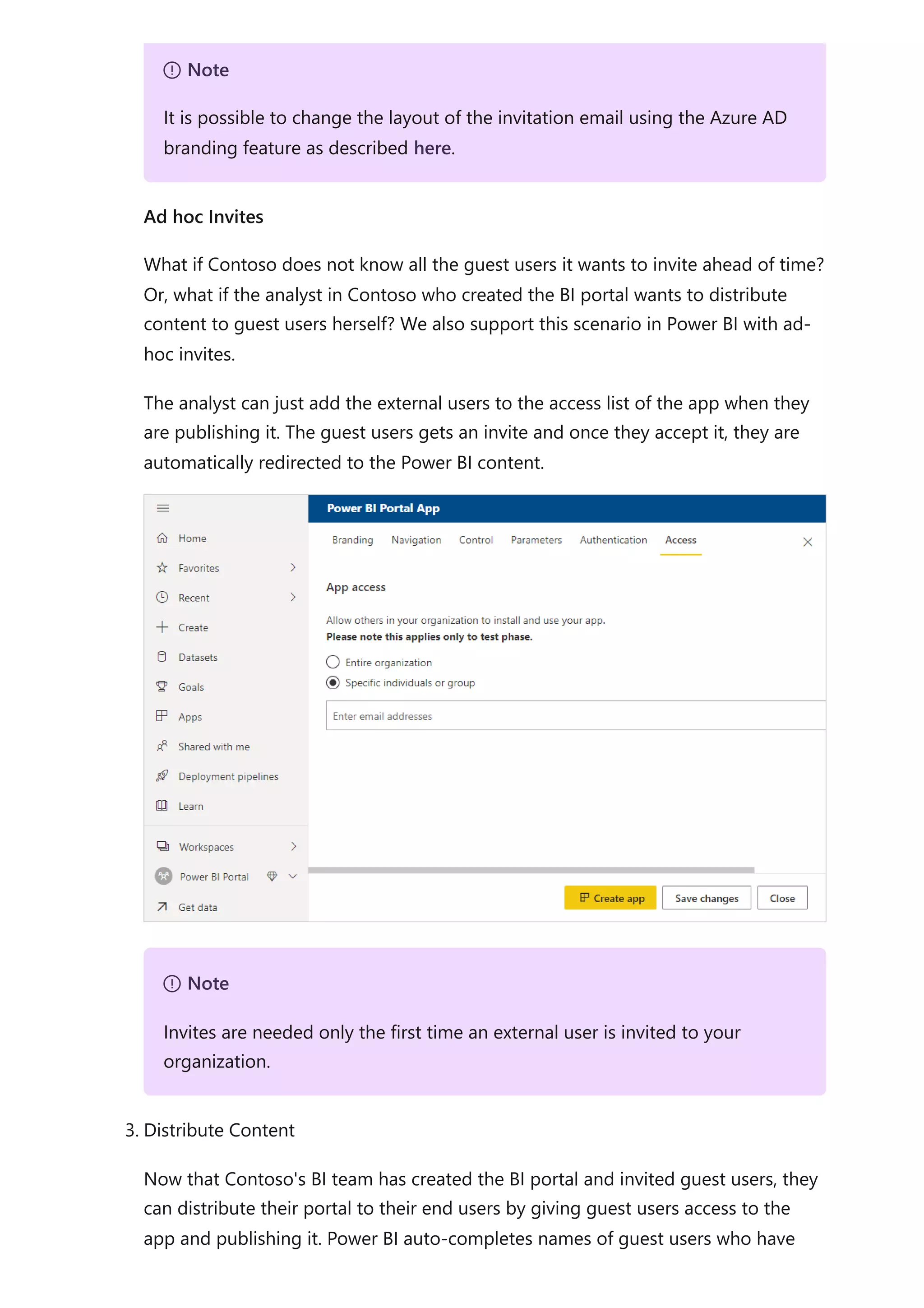
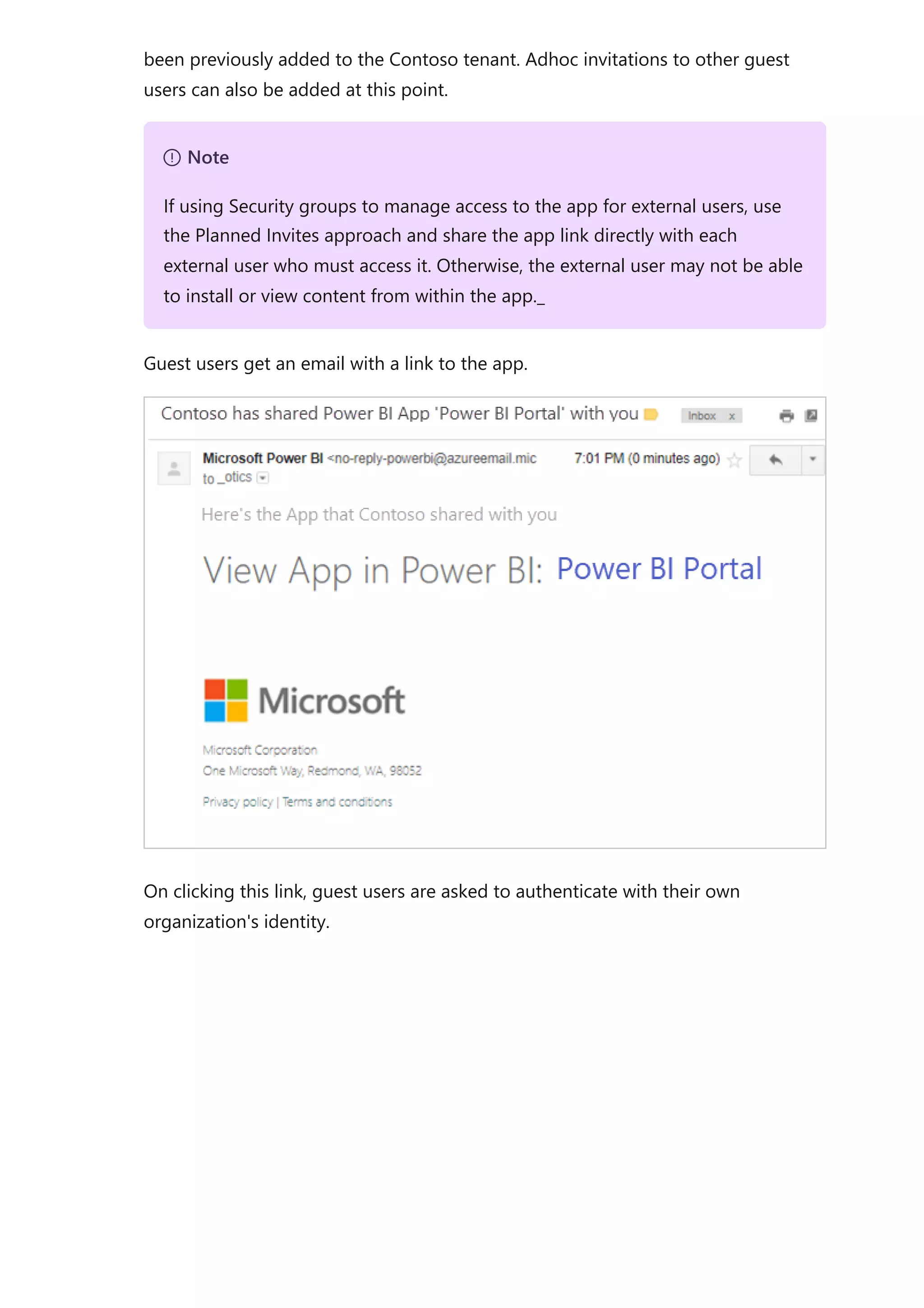
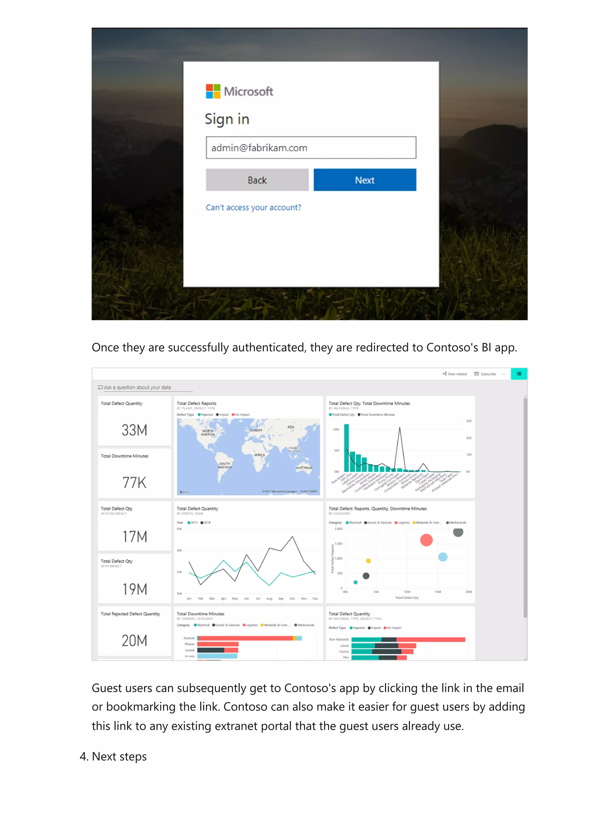
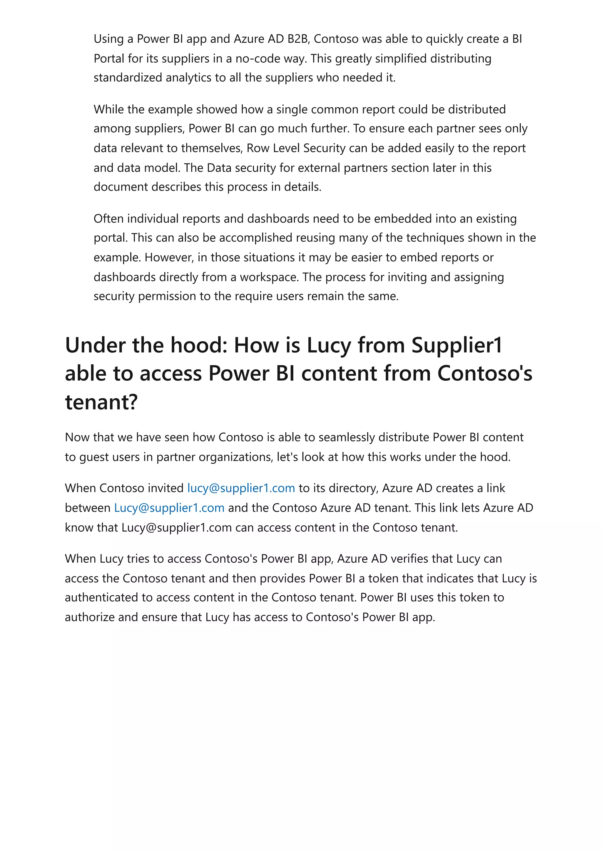
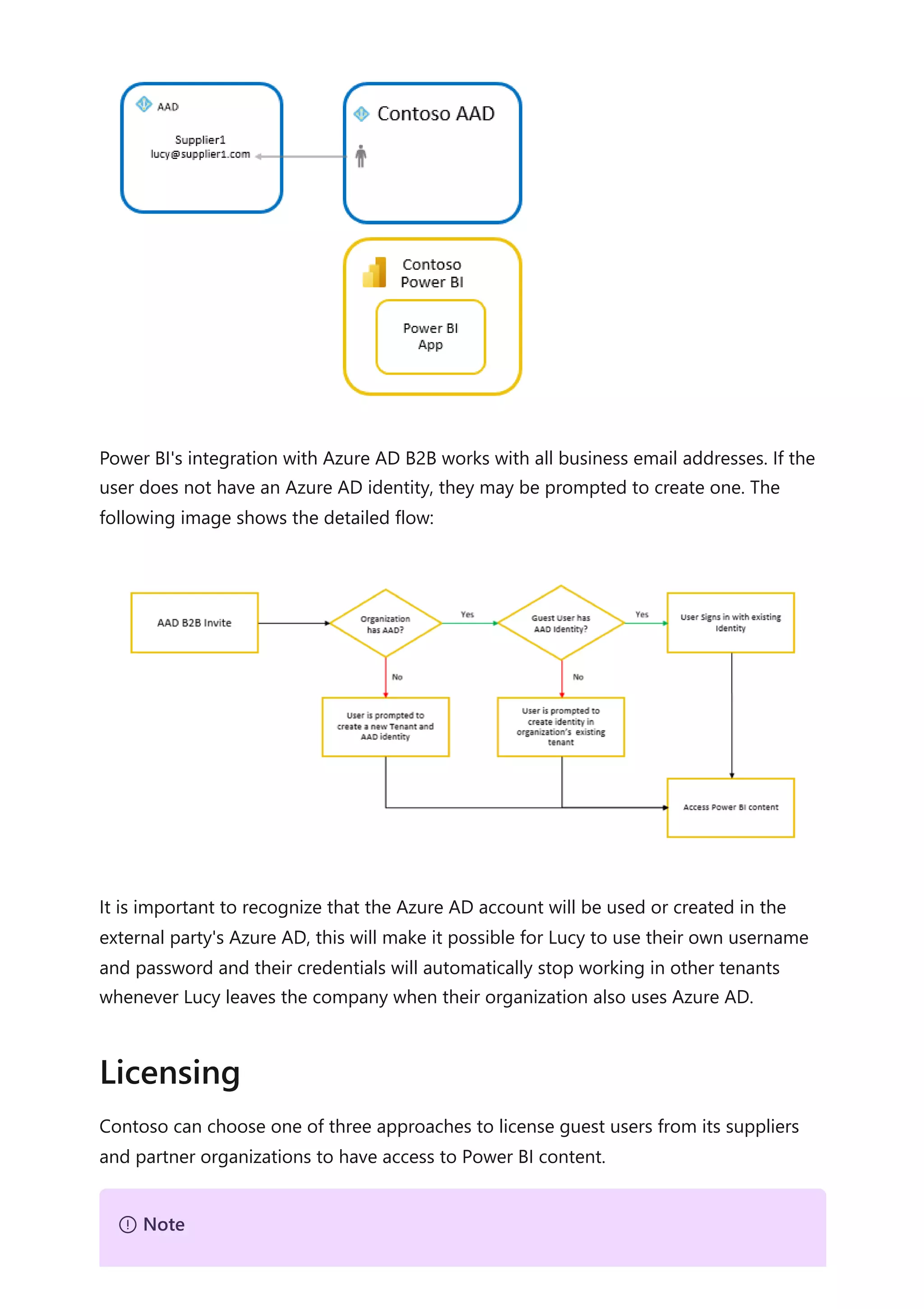
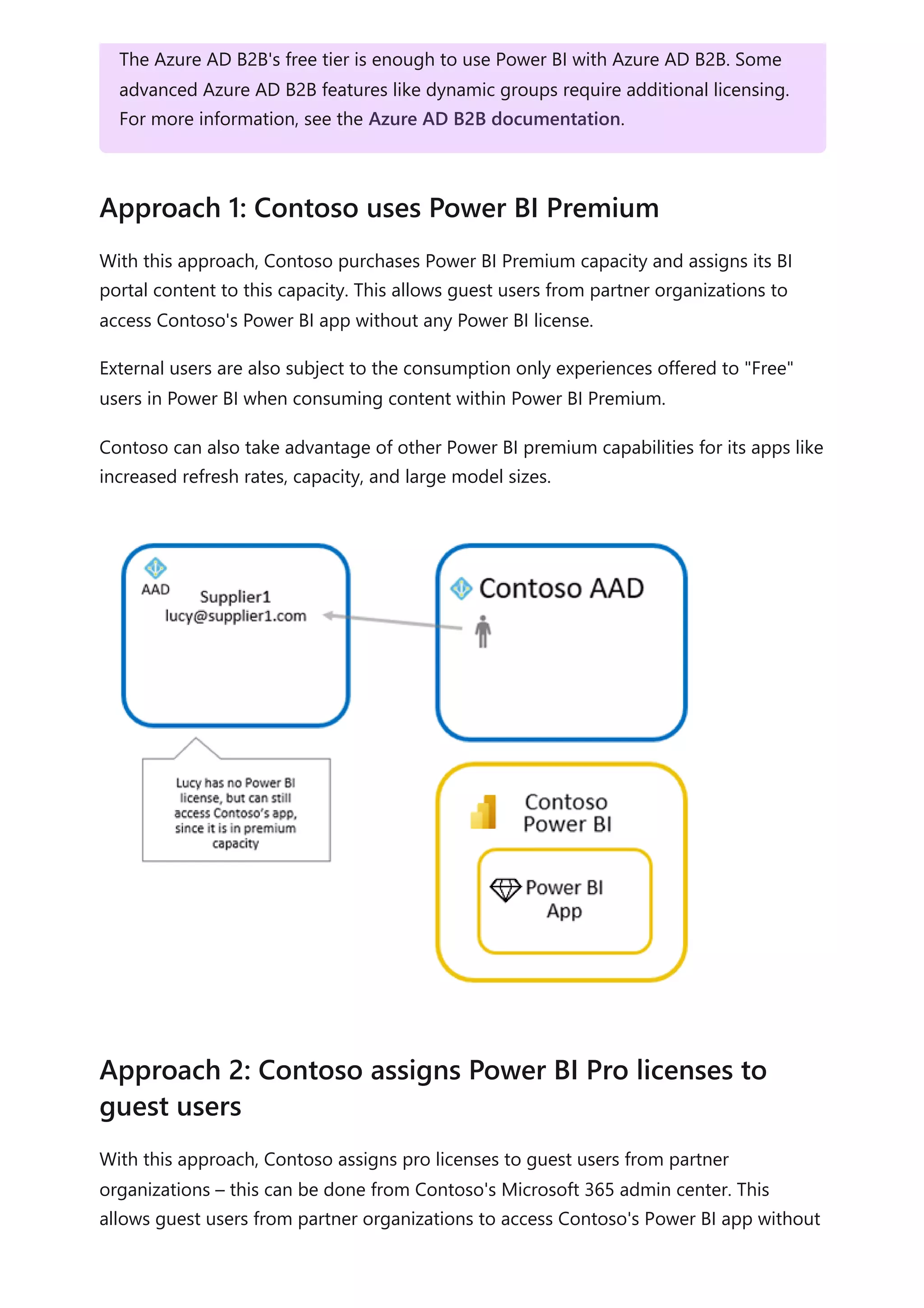
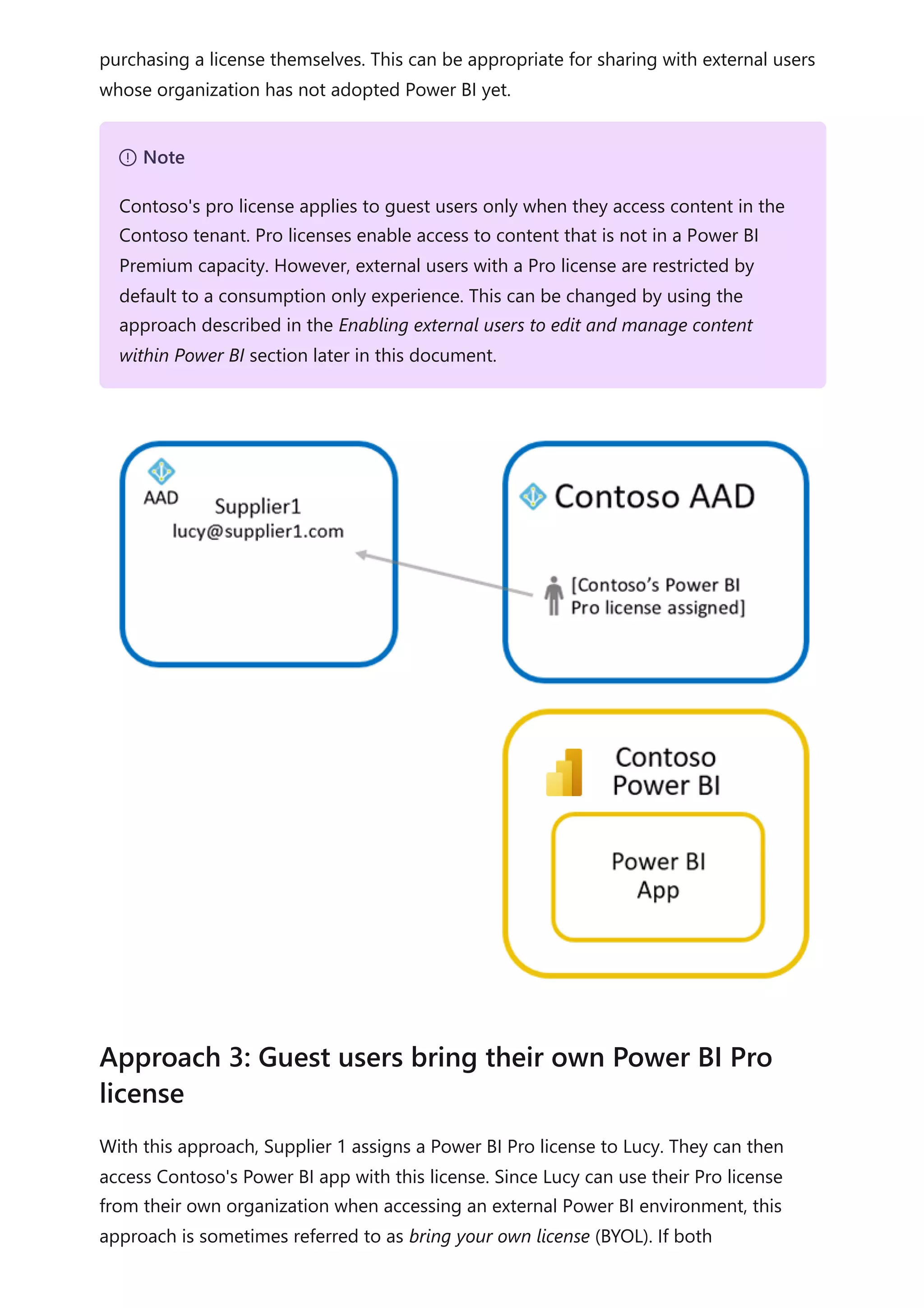
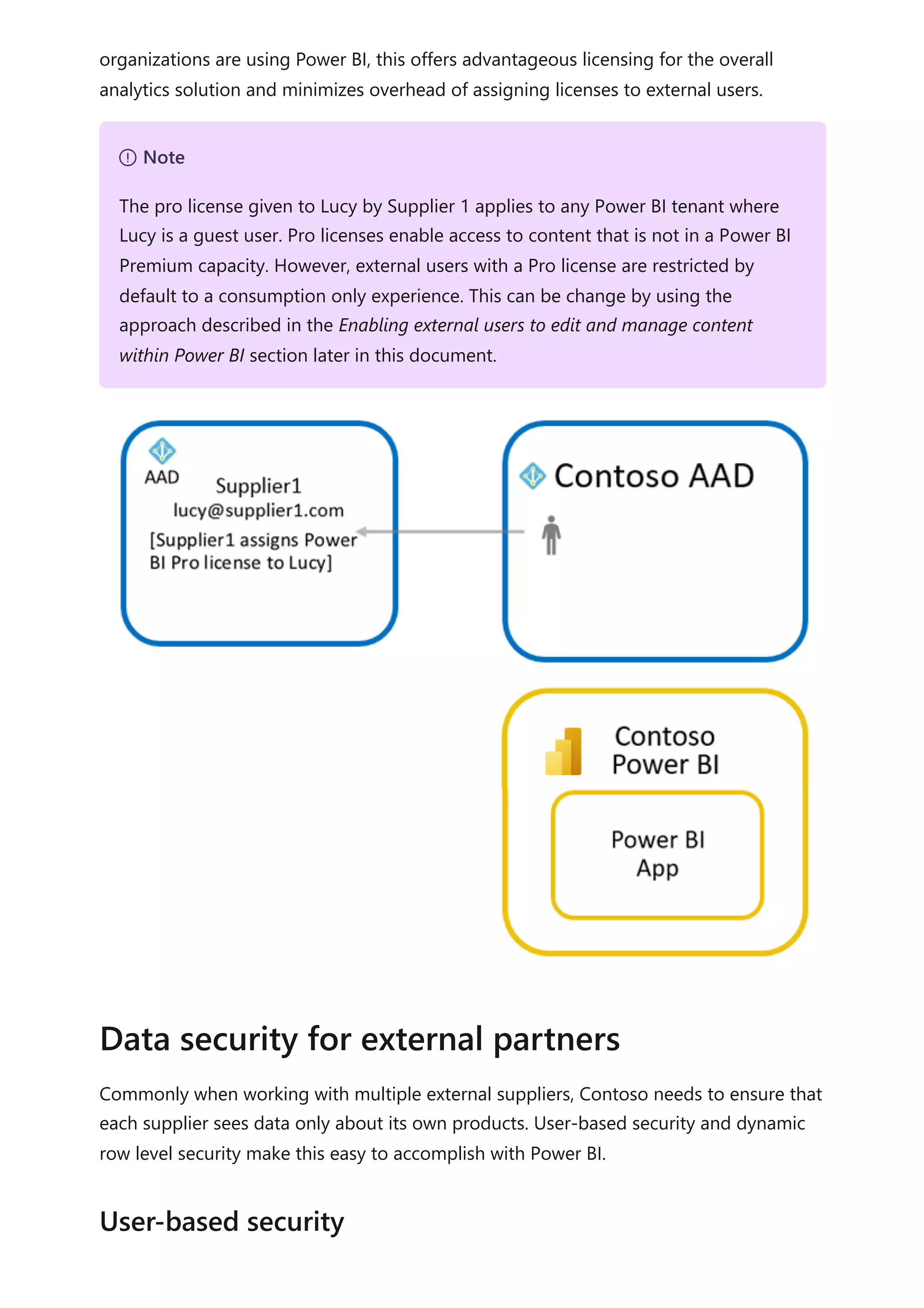
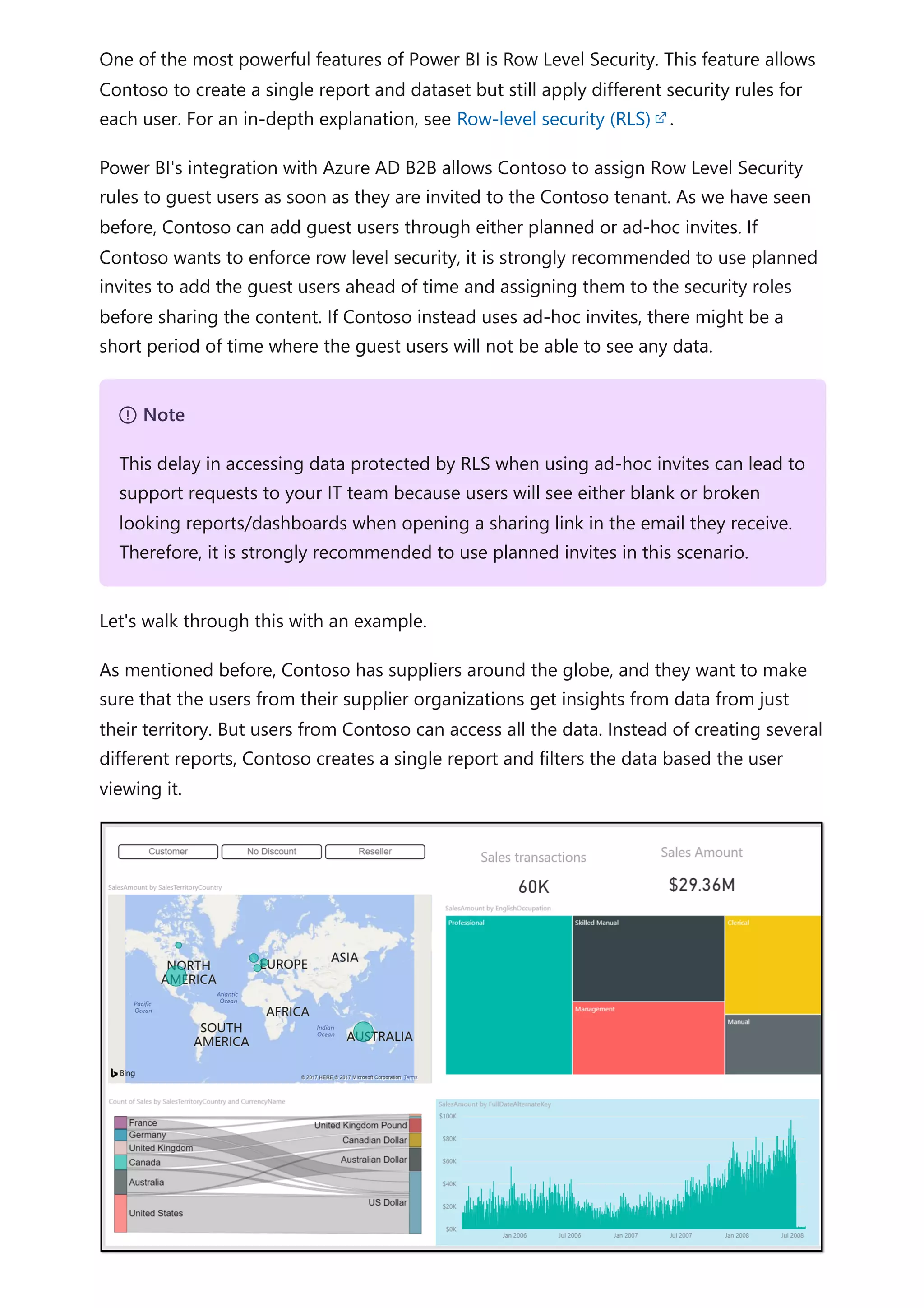
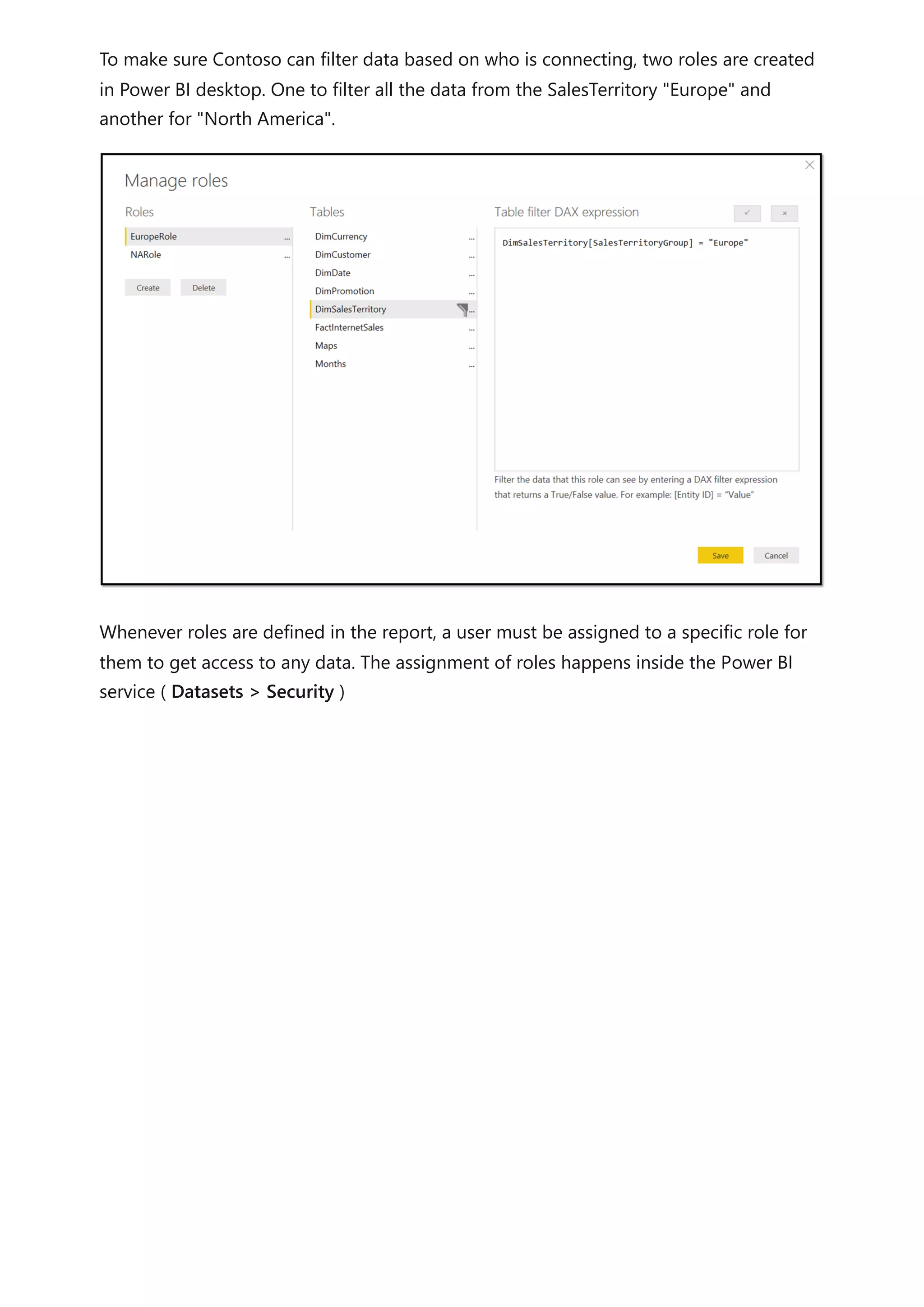
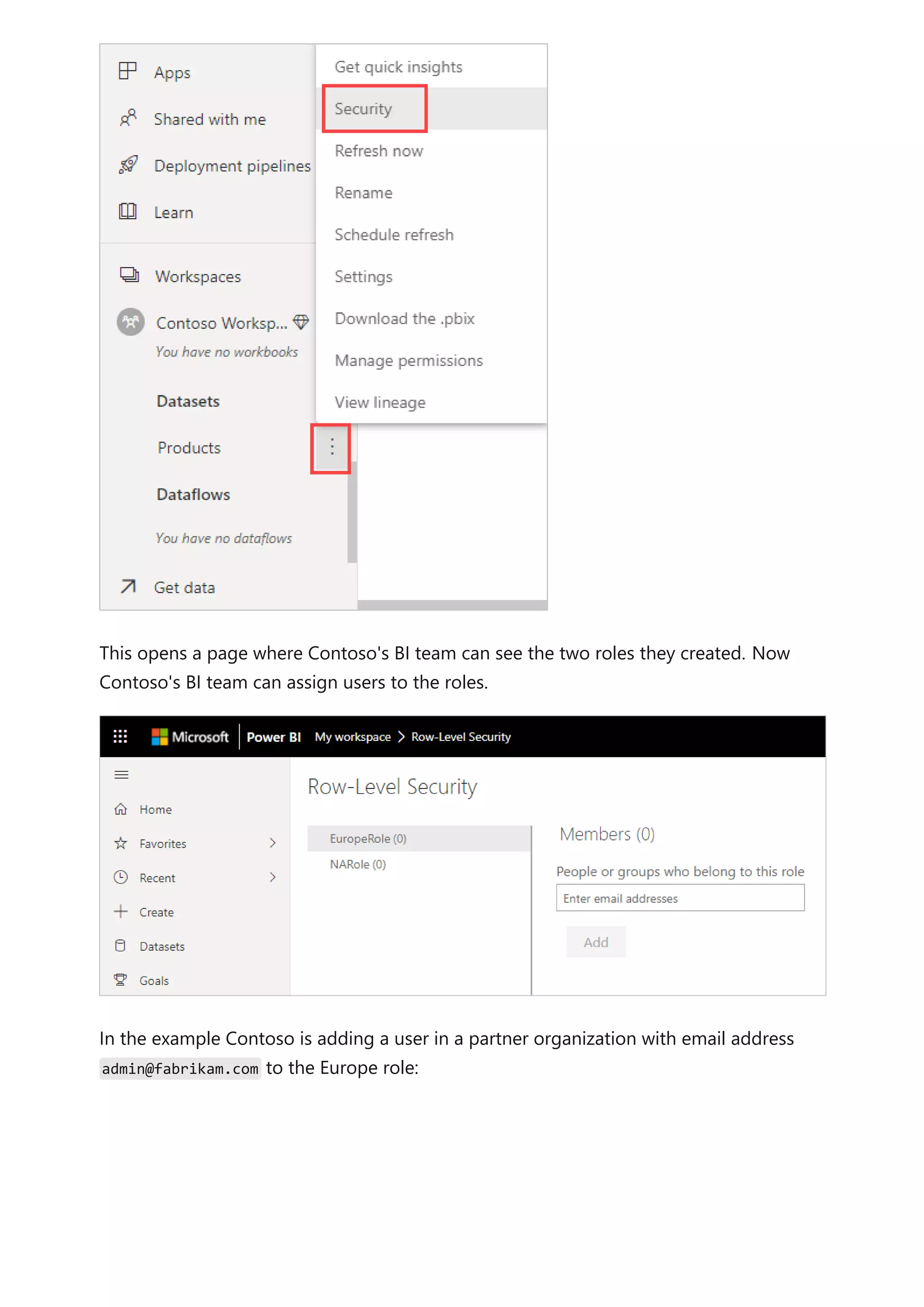
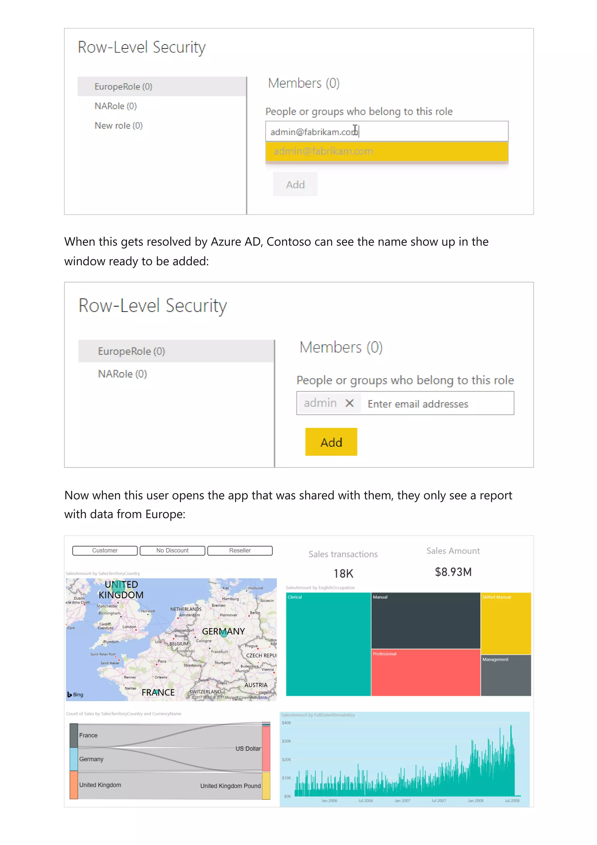
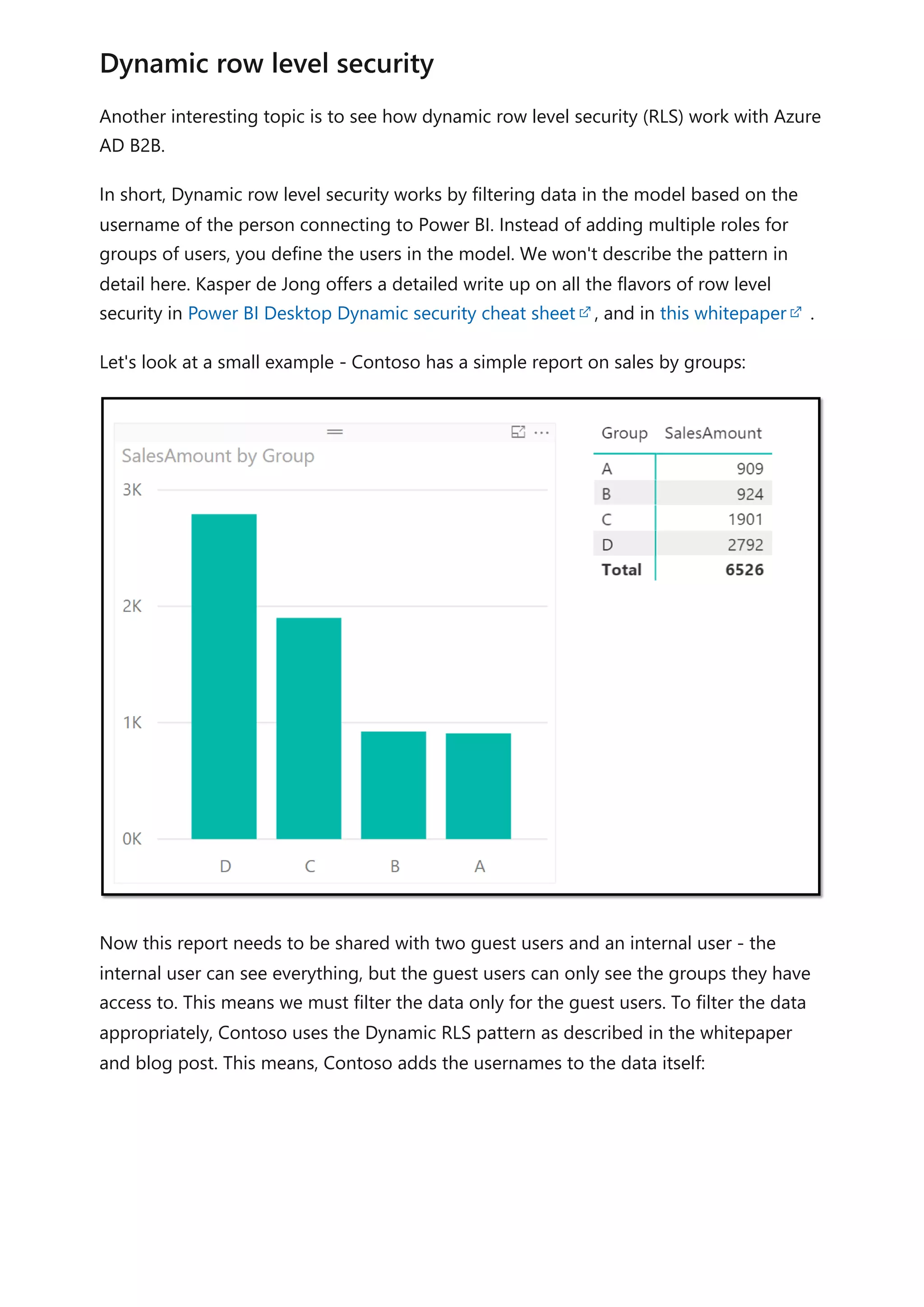
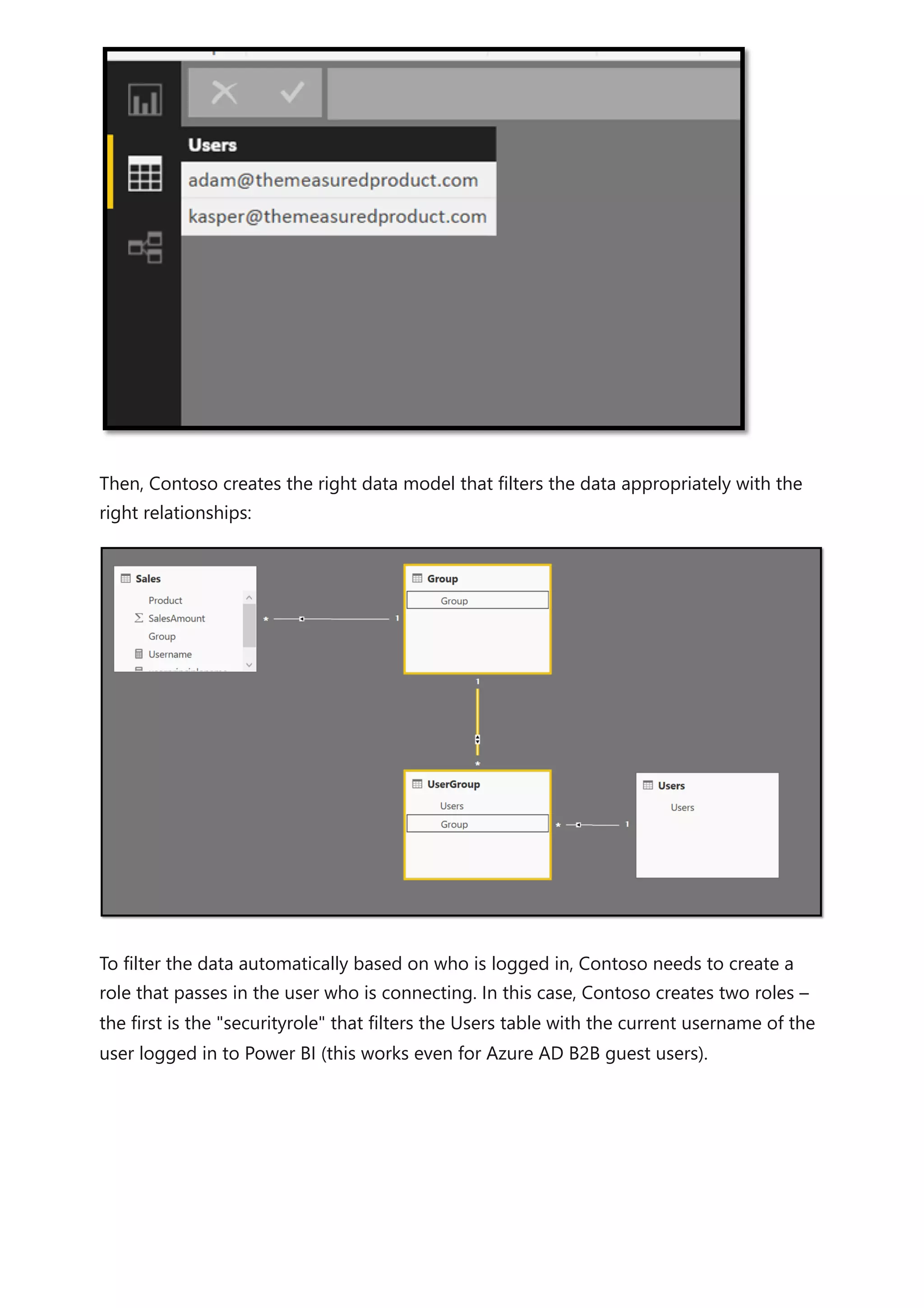
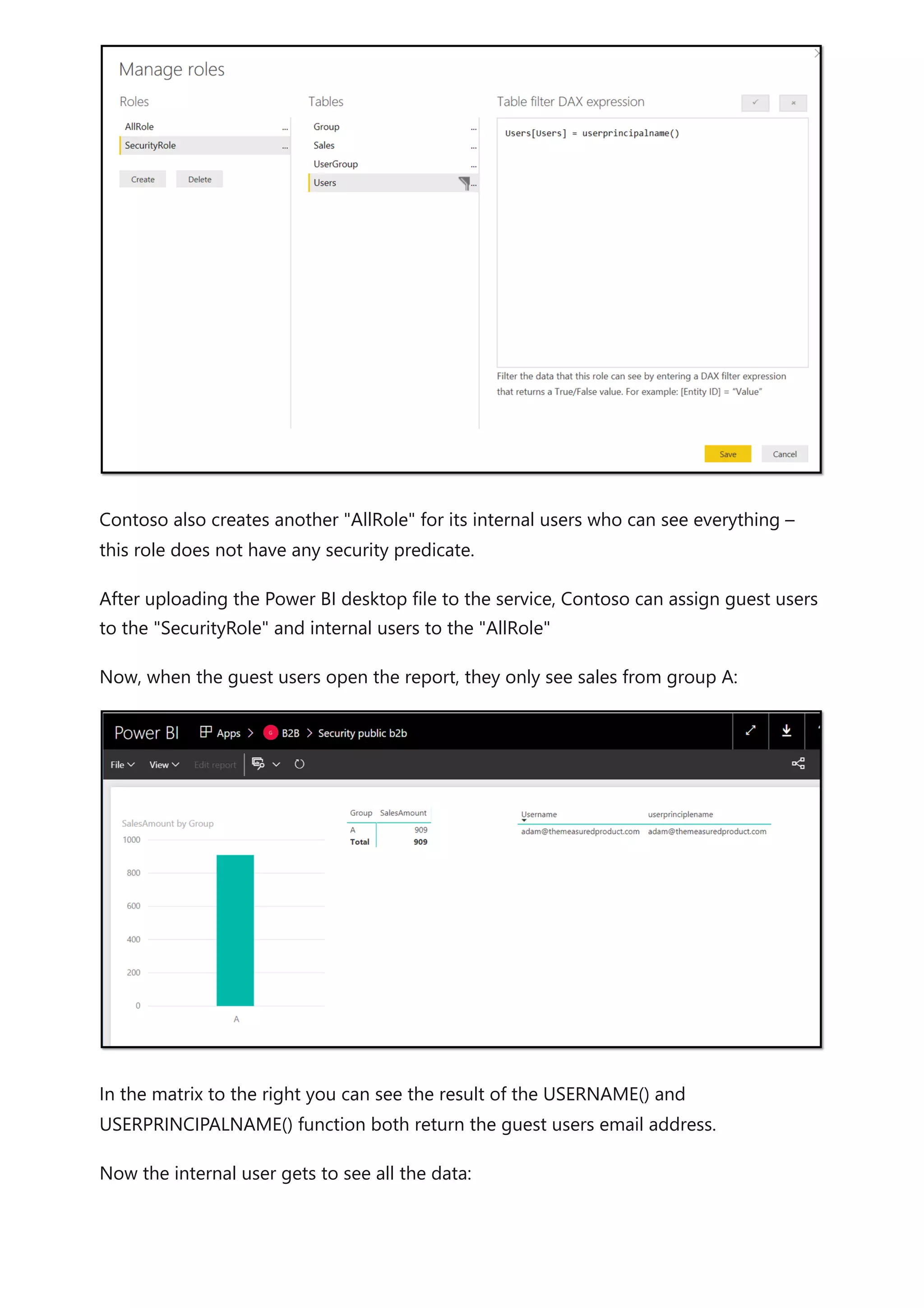
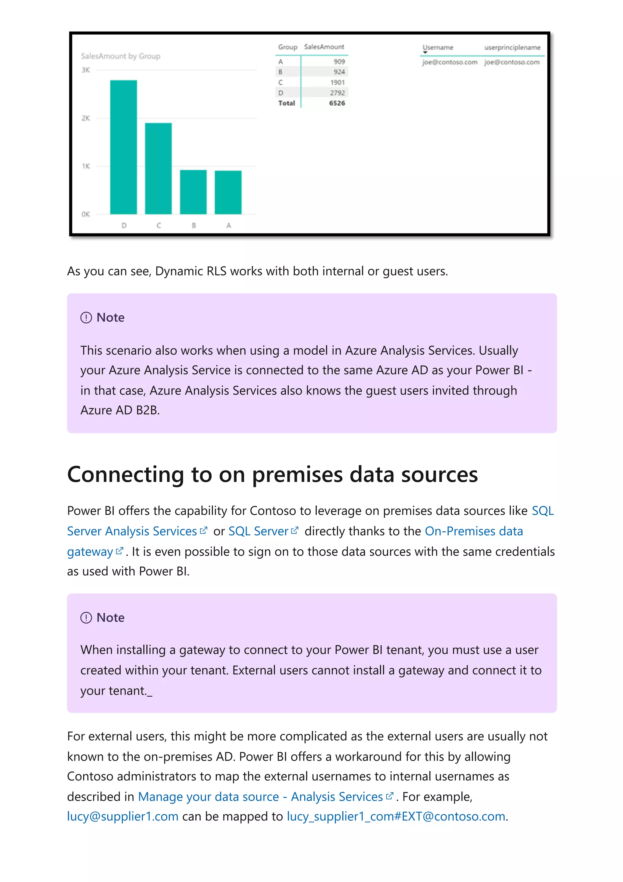
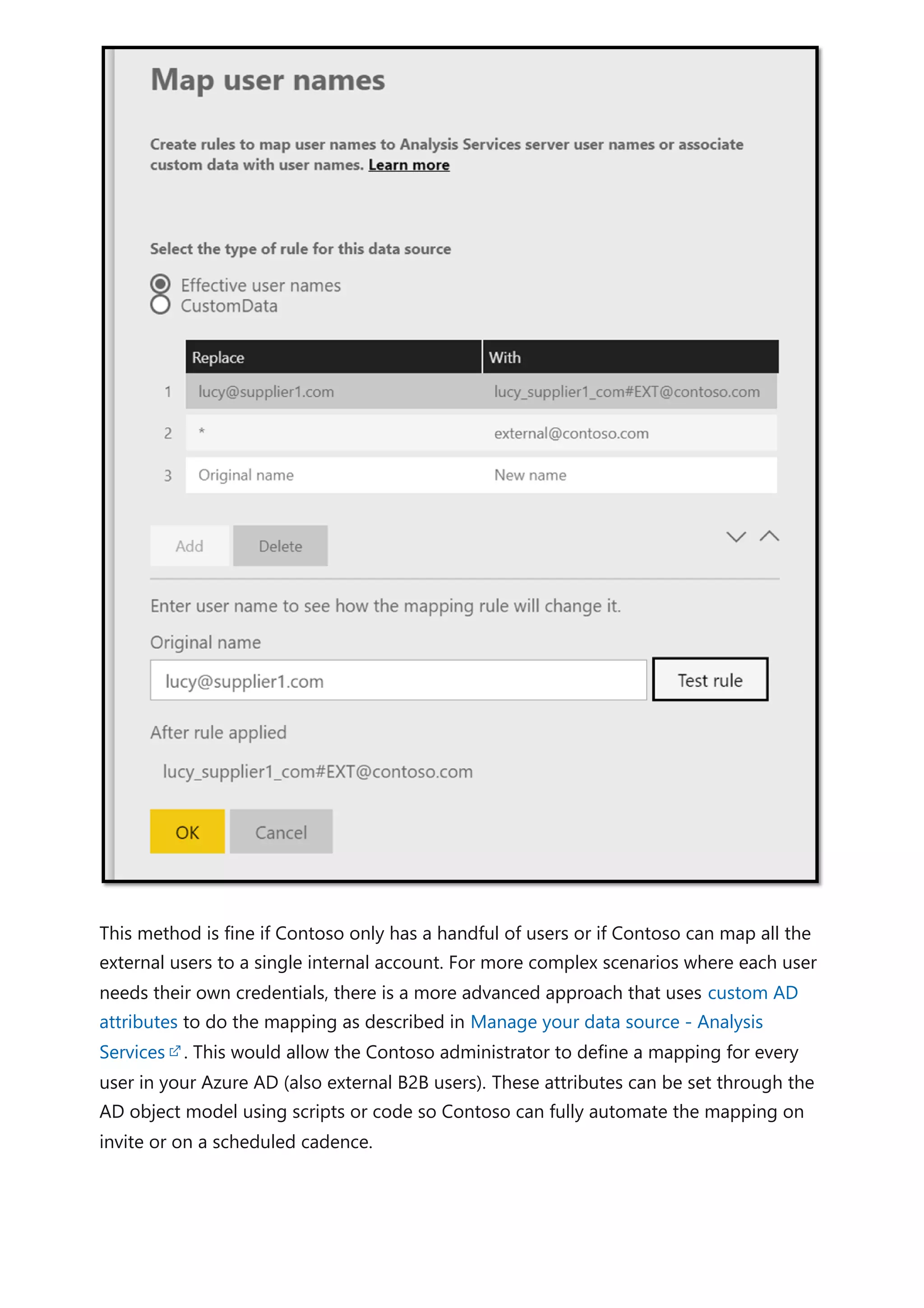
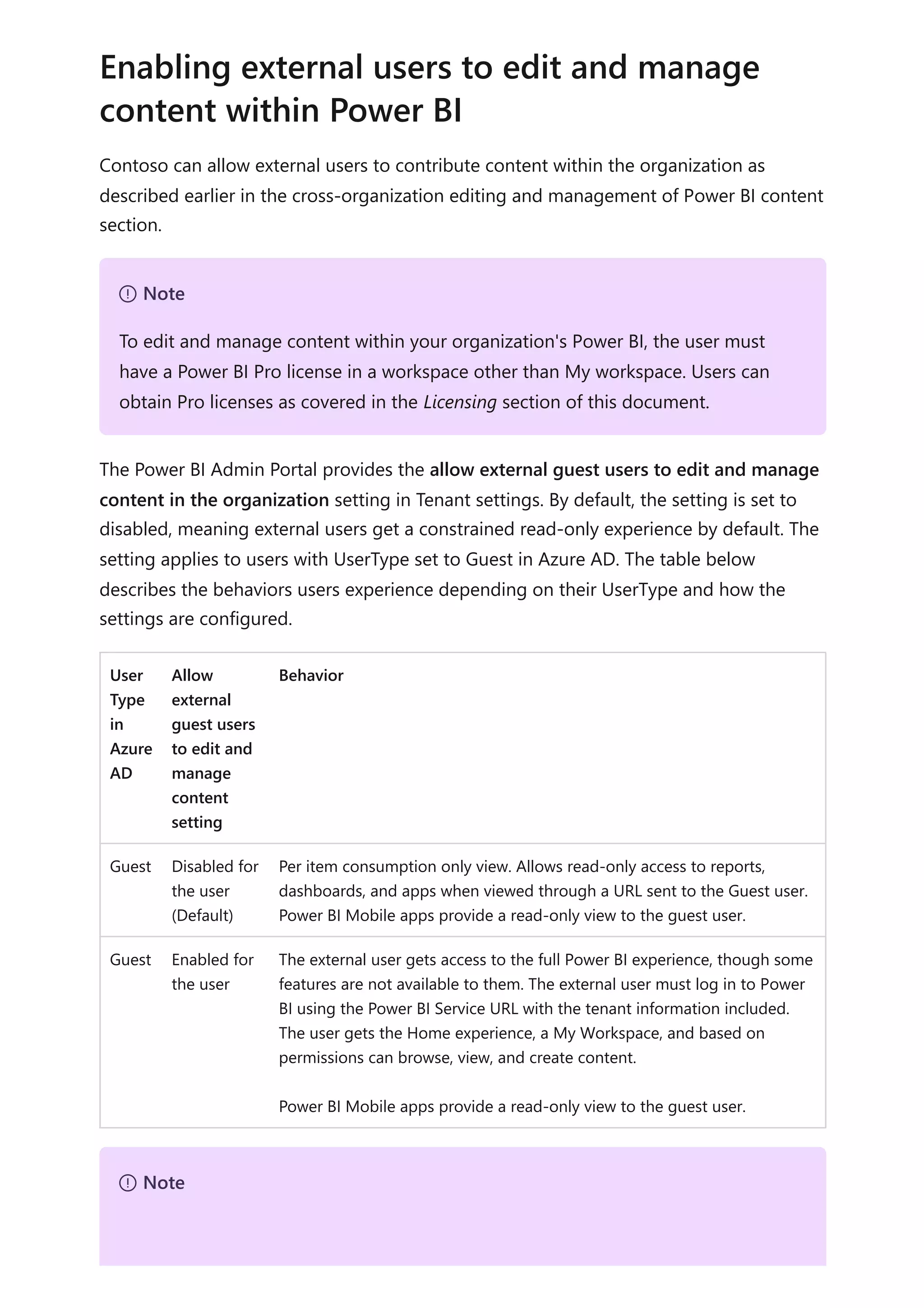
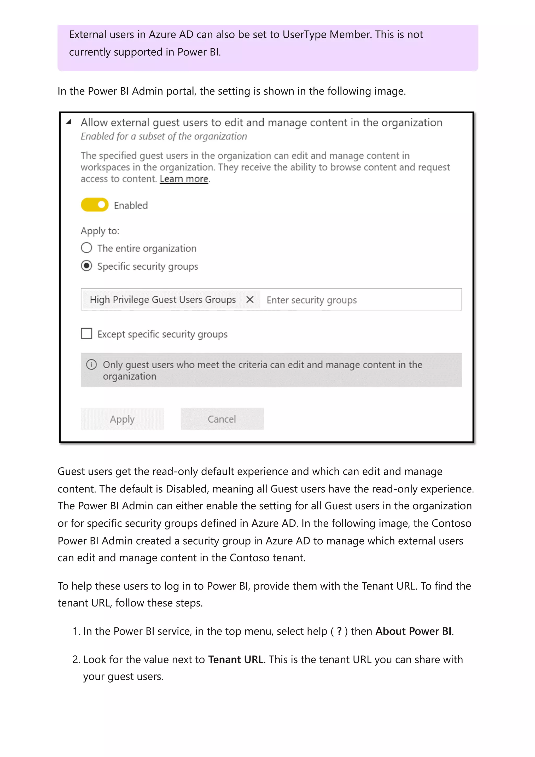
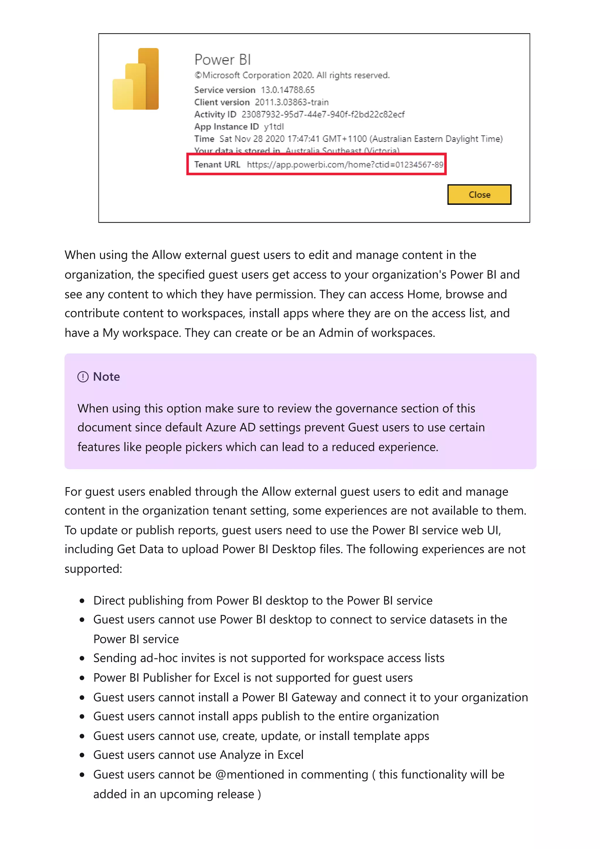
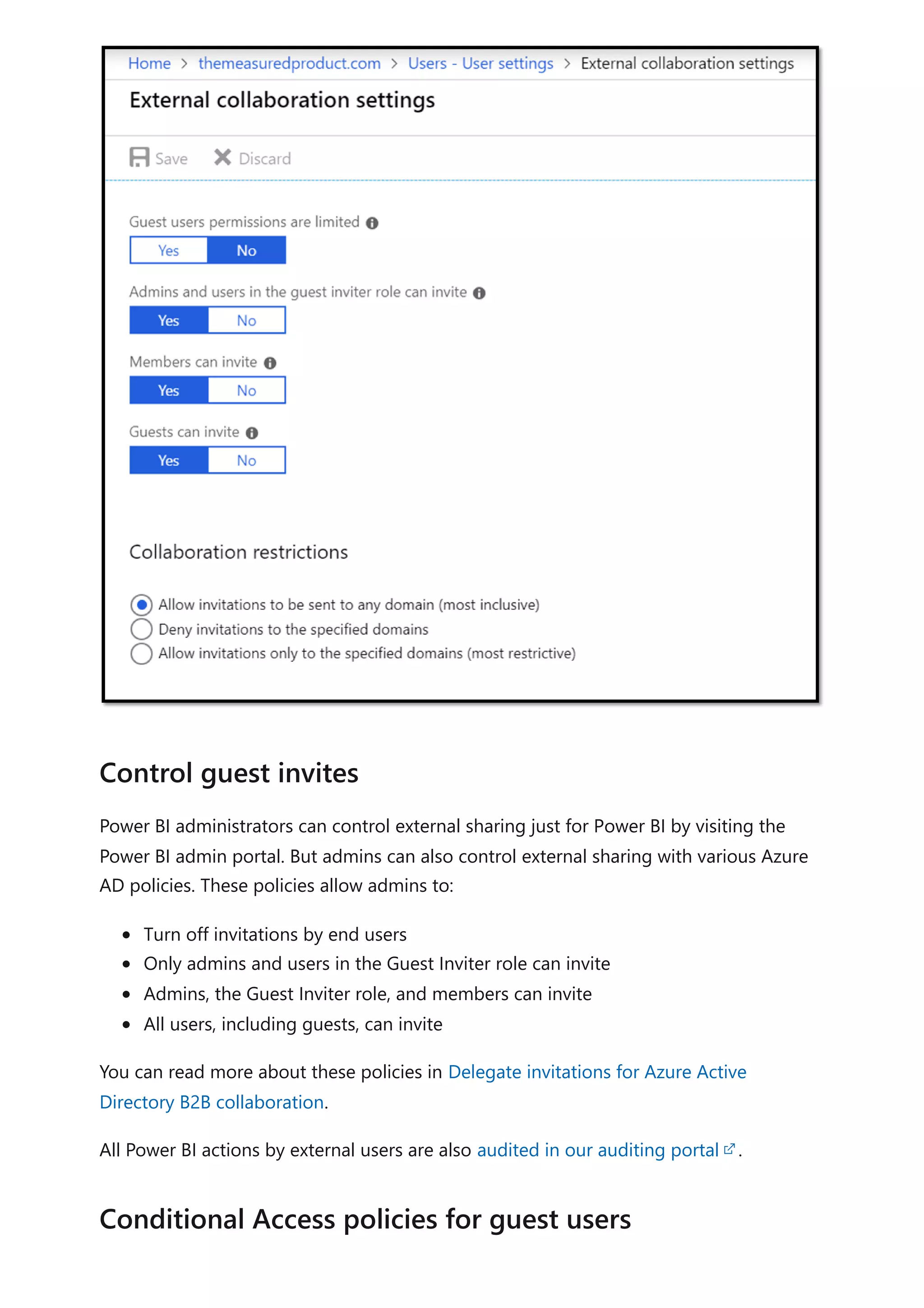
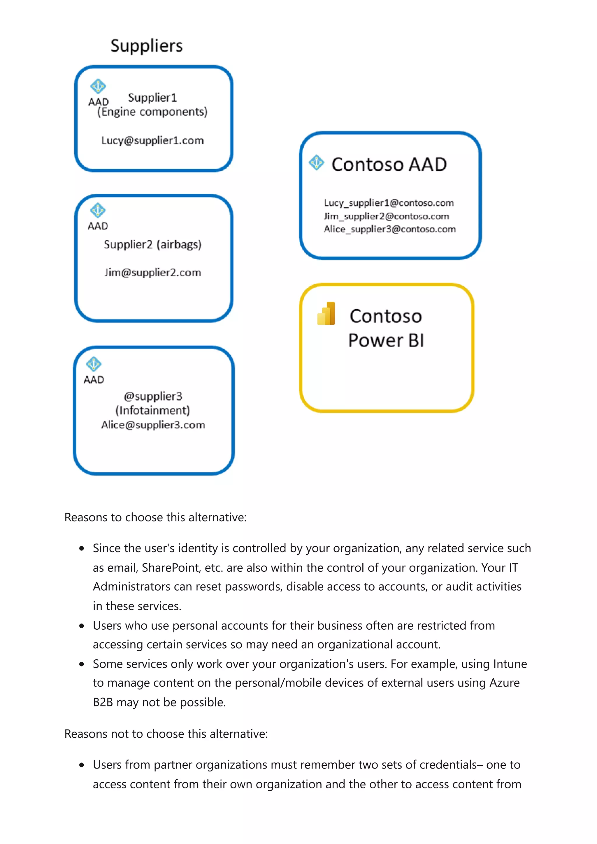


![[DSC Europe 25] Dunja Adzic Jovanovic - AI and Cybersecurity: Defending Data ...](https://cdn.slidesharecdn.com/ss_thumbnails/o1zylpbhrtwnixxq2xj8-7-251211083048-185086f6-thumbnail.jpg?width=640&height=640&fit=bounds)
![[DSC Europe 25] Behzad Hosseini - AI Agents in the Wild: Deploying Models tha...](https://cdn.slidesharecdn.com/ss_thumbnails/3qtejajvsjqrzwfept2c-10-251212103250-7f2b1068-thumbnail.jpg?width=640&height=640&fit=bounds)


![[DSC Europe 25] Katherine Forrest - AI NOW: Understanding the Velocity of Cha...](https://cdn.slidesharecdn.com/ss_thumbnails/wvvbruqfrci0sfq9xwgb-4-251212104007-e5ad1987-thumbnail.jpg?width=640&height=640&fit=bounds)
![[DSC Europe 25] Jon Dajci - Bridging TradFi and DeFi: Building the Future of ...](https://cdn.slidesharecdn.com/ss_thumbnails/fqmhfvlbqhkihjvqvhmu-7-251211083849-6af7e325-thumbnail.jpg?width=640&height=640&fit=bounds)


![[DSC Europe 25] Branko Dzakula - From Defense to Attack: How AI Redefines Cyb...](https://cdn.slidesharecdn.com/ss_thumbnails/80bdzdxpr3ky2g0qvyk9-8-251211083048-ce5fc1ee-thumbnail.jpg?width=640&height=640&fit=bounds)


![[DSC Europe 25] Branko Urosevic -Rethinking Financial Talent: Integrating Cod...](https://cdn.slidesharecdn.com/ss_thumbnails/8jjrus8ttko6qj64f58f-3-251212103250-642c6374-thumbnail.jpg?width=640&height=640&fit=bounds)


![[DSC Europe 25] Milan Sekuloski - Data, Defence, and Development: Cybersecuri...](https://cdn.slidesharecdn.com/ss_thumbnails/dfrkwwx4qly6atqpbl4z-4-251209104645-c3d4b0ca-thumbnail.jpg?width=640&height=640&fit=bounds)
