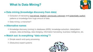
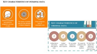
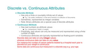
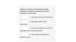
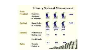
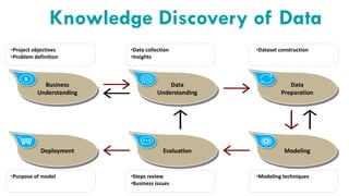
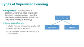
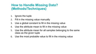
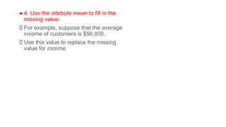
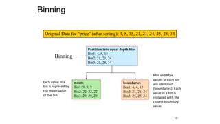
This document provides information about a course on data mining and data warehousing. It includes the vision and mission statements of the university and computer science department. It outlines the program outcomes, program educational objectives, and course outcomes. Finally, it provides a detailed syllabus covering topics like data preprocessing, frequent pattern mining, classification, clustering, and data warehousing. The goal is to teach students how to extract useful patterns from data through techniques like association rule mining, classification, and clustering.

1. IT30138 DATA MINING AND DATA
WAREHOUSE
Mr. Ankur Priyadarshi
Assistant Professor
Department of Computer Science and Information Technology
ankurpriyadarshi@cgu-odisha.ac.in
C. V. Raman Global University, Bhubaneswar, Odisha
Credits: 2

2. Vision and Mission
Vision of the C. V. Raman Global University: To emerge as a global leader in the arena of technical
education commensurate with the dynamic global scenario for the benefit of mankind.
Vision of the Department of CSE : To become a leader in providing high quality education and
research in the area of Computer Science, Information Technology, and allied areas.
Mission of C.V. Raman Global University :
❖ To provide state-of-art technical education in the undergraduate and
postgraduate levels;
❖ to work collaboratively with technical Institutes / Universities / Industries of
National and International repute;
❖ to keep abreast with latest technological advancements;
❖ to enhance the Research and Development activities”.
Mission of the Department of CSE:
M1: To develop human resource with sound theoretical and practical knowledge in the discipline of
Computer Science & Engineering.
M2: To work in groups for Research, Projects, and Co-Curricular activities involving modern methods,
tools and technology.
M3: To collaborate and interact with professionals from industry, academia, professional societies,
community groups for enhancement of quality of education.

3. Program Outcomes
❖ Engineering knowledge
❖ Problem analysis
❖ Design/development of solutions
❖ Conduct investigations of complex problems
❖ Modern tool usage
❖ The engineer and society
❖ Environment and Ethics
❖ Individual and team work
❖ Communication
❖ Project management and finance
❖ Life-long learning

4. Program Educational Objective (PEO)
PEO1- To provide the fundamental knowledge in mathematics, science and
engineering concepts for the development of engineering system
(Fundamental Knowledge).
PEO2- To apply current industry accepted computing practices and emerging
technologies to analyze, design, implement, test and verify high quality
computing systems and computer based solutions to real world problems
(Design and development).
PEO3- To enable the use of appropriate skill sets and its applications towards
social impacts of computing technologies in the career related activities (Skill
Set) and to produce Efficient team leaders, effective communicators and
capable of working in multi-disciplinary environment following ethical
values(Communication).
PEO4- To practice professionally and ethically in various positions of industry
or government and/or succeed in graduate (Professionalism (Societal
Contribution)

5. Course Outcomes
Upon successful completion of this course, students will be able to:
CO1: Identify data mining architecture and different pre-processing techniques
required for analysis of given dataset
CO2: Analyze frequent patterns, determine associations and correlations
CO3: Apply different classification and prediction to data mining applications
CO4: Use different clustering mechanisms for data mining
CO5: Use data warehouse and data mining techniques for numeric, textual, temporal
and unstructured data on the Web

6. Syllabus
Unit 1
Data Mining and Pre-processing (08 Hrs)
U1.1. Introduction: Need of Data Mining, Knowledge Discovery in Database (KDD), Architecture of Data
Mining System; Data Objects and Attribute Types, Statistical Description of Data, Data Visualization
U1.2.Data Preprocessing: Introduction to Data mining, Data mining Functionalities, Data preprocessing (data
summarization, data cleaning, data integration and transformation, data reduction– Feature selection and
extraction, dimensionality reduction, data discretization)
U1.3.Self-Study: Integration of Data Mining with a Database or Data Warehouse System, Issues in Data
Mining

7. LEARNING
OUTCOMES
Need of Data Mining
Growth of Data
What exactly is data
mining?
Technology
required for data
mining
History of data
mining

8. Why Data Mining?

9. A Quote on Data Mining
Dr. Penzias, a Nobel prize winner interviewed in
Computer World in January 1999, states concisely:
"Data mining will become more important, and companies
will throw away nothing about their customers because it
will be so valuable. If you're not doing this, you're out of
business."

10. Growth of Data

11. The Information Challenge
https://images.app.goo.gl/N8hekmd4BCqidnsJ6

12. 1960s
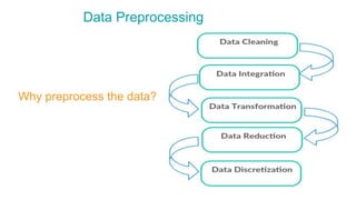
Data Collection
[Computers, Tape]
1970s
Data Access
Relational Database
1980s
Application oriented RDBMS
Object Oriented Model
1990s
Data Mining
Data Warehousing
2000s
Big Data Analytics
No-SQL
Evolution of Data Mining

13. Applications of Data Mining

14. Cyclone Forecasting
https://images.app.goo.gl/GdiLivTrGZe9aYJY8

15. Spam Detection
https://pepipost.com/tutorials/spam-filter/

16. Gmail Text Recommendation
https://ai.googleblog.com/2018/05/smart-compose
-using-neural-networks-to.html

17. E-Commerce Application

18. Clustering

19. Banking

20. What is mining?
Extraction of non-obvious, implicit, unknown and useful resources from planet.

21. What Is Data Mining?
● Data mining (knowledge discovery from data)
○ Extraction of interesting (non-trivial, implicit, previously unknown and potentially useful)
patterns or knowledge from huge amount of data
○ Data mining: a misnomer?
● Alternative names
○ Knowledge discovery (mining) in databases (KDD), knowledge extraction, data/pattern
analysis, data archeology, data dredging, information harvesting, business intelligence, etc.
● Watch out: Is everything “data mining”?
○ Simple search and query processing
○ (Deductive) expert systems

22. Quiz of the Day
Scan/Copy link it and give your choice
https://forms.gle/m97uenx3zYtKEV4y9

23. OPTION 1
Unknown
Answer - NO
OPTION 2
Implicit
Answer -
No
OPTION 3
Useful
Answer -
No
OPTION 4
Obvious
Answer -
yes
Answer of the Day
Q: Which of the following keyword is not associated with Data mining?

24. Getting to Know Your Data
(Data Objects and Attribute Types)
24
Unit 1: Data and Data Preprocessing

25. 25
Types of Data Sets
● Record
○ Relational records
○ Data matrix, e.g., numerical
matrix, crosstabs
○ Document data: text documents:
term-frequency vector
○ Transaction data
● Graph and network
○ World Wide Web
○ Social or information networks
○ Molecular Structures
● Ordered
○ Video data: sequence of images
○ Temporal data: time-series
○ Sequential Data: transaction sequences
○ Genetic sequence data
● Spatial, image and multimedia:
○ Spatial data: maps
○ Image data:
○ Video data:

26. 26
Record Data

27. 27
Data Matrix

28. 28
Transaction Data

29. 29
Graph Data

30. Spatial Data

31. Sequence Data

32. Data Objects
● Data sets are made up of data objects.
● A data object represents an entity.
● Examples:
○ sales database: customers, store items, sales
○ medical database: patients, treatments
○ university database: students, professors, courses
● Also called samples , examples, instances, data points,
objects, tuples.
● Data objects are described by attributes.
● Database rows -> data objects; columns ->attributes.

34. Types of Variables / Attributes
●Variables:
○Qualitative
■Ordinal or Nominal
○Quantitative (or numeric)
■Discrete(Integer) or Continuous
🡪some numeric data are discrete and some are continuous
For statistical analysis, qualitative data can be converted
into discrete numeric data(Quantitative)
34

35. Quantitative Data
▪ Quantitative or numerical data arise when the observations are counts or
measurements.
▪ Quantitative data is information about quantities; that is, information that can
be measured and written down with numbers. Some examples
of quantitative data are your height, your shoe size, and the length of your
fingernails.
▪ Discrete data can be numeric -- like numbers of apples (i.e., Data that can
only take certain values. For example: the number of students in a class -you
can't have half a student).
▪ Discrete data can also be categorical -- like red or blue, or male or female, or
good or bad.
35

36. ● The table shows a part of some (hypothetical) data on a group of 48
subjects.
'Age' and 'income' are continuous numeric variables,
'age group' is an ordinal qualitative variable,
and 'sex' is a nominal qualitative variable.
● The ordinal variable 'age group' is created from the continuous variable
'age' using five categories:
age group = 1 if age is less than 20;
age group = 2 if age is 20 to 29;
age group = 3 if age is 30 to 39;
age group = 4 if age is 40 to 49;
age group = 5 if age is 50 or more
36

37. Types of Data :
Nominal, Ordinal, Interval and Ratio
Nominal:
▪Nominal scales are used for labeling variables, without any quantitative
value.
▪“Nominal” scales could simply be called “labels.”
▪No specific order
▪A good way to remember all of this is that “nominal” sounds a lot like
“name” and nominal scales are kind of like “names” or labels.
37

39. Ordinal Data
▪Ordinal scales are typically measures of non-numeric concepts like
satisfaction, happiness, ratings etc.
▪“Ordinal” is easy to remember because is sounds like “order” and
that’s the key to remember with “ordinal scales”–it is the order that
matters, but that’s all you really get from these.
39

40. Ordinal Data

44. Interval
▪Interval scales are numeric scales in which we know not only the order, but
also the exact differences between the values.
▪The classic example of an interval scale is Celsius temperature because
the difference between each value is the same.
▪For example, the difference between 60 and 50 degrees is a measurable
10 degrees, as is the difference between 80 and 70 degrees.
▪Time is another good example of an interval scale in which
the increments are known, consistent, and measurable.
44

45. Ratio:
▪ Ratio data has all properties of interval data such as – data should have numeric
values, a distance between the two points are equal etc. but, unlike interval data
where zero is arbitrary, in ratio data, zero is absolute.
▪ Ratio data has a defined zero point.
● Income, height, weight, annual sales, market share, product defect rates, time to
repurchase, unemployment rate, and crime rate are examples of ratio data.
▪ A very good example of ratio data is the measurement of heights. Height could
be measured in centimeters, meters, inches or feet. It is not possible to have a
negative height. When comparing to interval data for example temperature can
be – 10-degree Celsius but height cannot be in negative.
▪ Ratio data can be multiplied and divided, this is one of the major differences
between ratio data and interval data, which can only be added and subtracted.
45

46. Binary Attribute
● Binary
○ Nominal attribute with only 2 states (0 and 1)
○ Symmetric binary: both outcomes equally important
■ e.g., gender
○ Asymmetric binary: outcomes not equally important.
■ e.g., medical test (positive vs. negative)
■ Convention: assign 1 to most important outcome (e.g., HIV positive)

47. Discrete vs. Continuous Attributes
● Discrete Attribute
○ Has only a finite or countably infinite set of values
■ E.g., zip codes, profession, or the set of words in a collection of documents
○ Sometimes, represented as integer variables
○ Note: Binary attributes are a special case of discrete attributes
● Continuous Attribute
○ Has real numbers as attribute values
■ E.g., temperature, height, or weight
○ Practically, real values can only be measured and represented using a finite
number of digits
○ Continuous attributes are typically represented as floating-point variables
Discrete data can take on only integer values
whereas continuous data can take on any value.
For instance the number of cancer patients treated by a hospital each year is
discrete but your weight is continuous.
Some data are continuous but measured in a discrete way e.g. your age.

51. Case Study-1
● Let us take an example of “200 meter race” in a tournament where three runners are
participating from three different branches of CGU.
● Each runner is assigned a number (displayed in uniform) to differentiate from each
other. The number displayed in the uniform to identify runners is an example of
nominal scale.
● Once the race is over, the winner is declared along with the declaration of first runner
up and second runner up based on the criteria that who reaches the destination first,
second and last. The rank order of runners such as “second runner up as 3”, “first
runner up as 2” and the “winner as 1” is an example of ordinal scale.
● During the tournament, judge is asked to rate each runner on the scale of 1–10
based on certain criteria. The rating given by the judge is an example of interval
scale.
● The time spent by each runner in completing the race is an example of ratio scale.

53. Evaluation
Business
Understanding
Data
Understanding
Data
Preparation
Modeling
Deployment
•Project objectives
•Problem definition
•Data collection
•Insights
•Dataset construction
•Purpose of model •Steps review
•Business issues
•Modeling techniques
Knowledge Discovery of Data

54. Interpretation/Evaluation
Data Mining
Transformation
Pre-processing
Selection
Target data
Processed data
Transformed data
Patterns
Knowledge
•Data visualization and result interpretation
•Model with algorithms such as clustering, regression
and classification
•Dimension-reduction
•Factor analysis
•Difference, or taking logarithm to be Normalization
•Data collection and sampling
•Correlation analysis
Knowledge Discovery of Data

55. 55
Data Preprocessing
Why preprocess the data?

56. 56
Why Data Preprocessing?
●Data in the real world is dirty
○incomplete: lacking attribute values, lacking
certain attributes of interest, or containing only
aggregate data
■ e.g., occupation=“ ”
○noisy: containing errors or outliers
■ e.g., Salary=“-10”
○inconsistent: containing discrepancies in codes
or names
■ e.g., Age=“42” Birthday=“03/07/1997”
■ e.g., Was rating “1,2,3”, now rating “A, B, C”
■ e.g., discrepancy between duplicate records

57. 57
Why Is Data Dirty?
● Incomplete data may come from
○ “Not applicable” data value when collected
○ Different considerations between the time when the data was
collected and when it is analyzed.
○ Human/hardware/software problems
● Noisy data (incorrect values) may come from
○ Faulty data collection instruments
○ Human or computer error at data entry
○ Errors in data transmission
● Inconsistent data may come from
○ Different data sources
○ Functional dependency violation (e.g., modify some linked data)
● Duplicate records also need data cleaning

58. 58
Why Is Data Preprocessing Important?
● No quality data, no quality mining results!
○ Quality decisions must be based on quality data
■ e.g., duplicate or missing data may cause incorrect or even
misleading statistics.
○ Data warehouse needs consistent integration of quality
data
● Data extraction, cleaning, and transformation comprises
the majority of the work of building a data warehouse

59. 59
Multi-Dimensional Measure of Data Quality
● A well-accepted multidimensional view:
○ Accuracy
○ Completeness
○ Consistency
○ Timeliness
○ Believability
○ Value added
○ Interpretability
○ Accessibility
● Broad categories:
○ Intrinsic, contextual, representational, and accessibility

60. 60
Major Tasks in Data Preprocessing
● Data cleaning
○ Fill in missing values, smooth noisy data, identify or remove
outliers, and resolve inconsistencies
● Data integration
○ Integration of multiple databases, data cubes, or files
● Data transformation
○ Normalization and aggregation
● Data reduction
○ Obtains reduced representation in volume but produces the same
or similar analytical results
● Data discretization
○ Part of data reduction but with particular importance, especially for
numerical data

61. 4
Topic
Topic
3
Topic
2
Topic
1
Types of
Learning
Supervised
Learning
Unsupervised
Learning
Classification
vs Regression
Outline

62. Data Mining Functionalities
62

63. 63
Types of Learning

64. Supervised Learning
●The training data includes both Inputs and Labels(Targets)
●what are Inputs and Labels(Targets)?? for example addition of two
numbers a=5,b=6 result =11, Inputs are 5,6 and Target is 11

65. Unsupervised Learning
●The training data does not include Targets here so we don’t tell the system
where to go , the system has to understand itself from the data we give.

66. Reinforcement Learning
●Though both supervised and reinforcement learning use mapping between input
and output, unlike supervised learning where the feedback provided to the agent
is correct set of actions for performing a task, reinforcement learning
uses rewards and punishments as signals for positive and negative behavior

67. ●An RL problem can be best explained through games.
●Goal : to eat food
●Environment - Grid
●Reward for eating food
●Punishment - if killed by Ghost

68. Types of Supervised Learning
●Regression: This is a type of
problem where we need to predict
the continuous-response value (ex :
above we predict number which can
vary from -infinity to +infinity)
●Some examples are
○ what is the price of house in a specific city?
○ what is the value of the stock?
○ how many total runs can be on board in a
cricket game?

69. ●Classification: This is a type of problem where we predict the categorical
response value where the data can be separated into specific “classes” (ex:
we predict one of the values in a set of values).
●Some examples are :
○ this mail is spam or not?
○ will it rain today or not?
○ is this picture a cat or not?
○ Basically ‘Yes/No’ type questions called binary classification.
○ Other examples are :
○ this mail is spam or important or promotion?
○ is this picture a cat or a dog or a tiger?
○ This type is called multi-class classification.

70. Classification vs Regression

71. Unsupervised Learning
●Clustering: This is a type of problem where
we group similar things together.
●Bit similar to multi class classification but
here we don’t provide the labels, the system
understands from data itself and cluster the
data.
●Some examples are :
○ given news articles, cluster into different types of
news
○ given a set of tweets ,cluster based on content of
tweet
○ given a set of images, cluster them into different
objects

72. Data Cleaning and Integration

73. How to Handle Missing Data?
(Methods/Techniques)
1. Ignore the tuple
2. Fill in the missing value manually
3. Use a global constant to fill in the missing value
4. Use the attribute mean to fill in the missing value
5. Use the attribute mean for all samples belonging to the same
class as the given tuple
6. Use the most probable value to fill in the missing value

74. How to Handle Missing Data? (Methods)
1. Ignore the tuple: This is usually done when the class label is missing
(assuming the mining task involves classification).
This method is not very effective, unless the tuple contains several attributes
with missing values.
It is especially poor when the percentage of missing values per attribute varies
considerably.

75. 2. Fill in the missing value manually
● In general, this approach is time-consuming and may not be feasible given
a large data set with many missing values.

76. ● 3. Use a global constant to fill in the missing value:
Replace all missing attribute values by the same constant, such as
a label like “Unknown” .
If missing values are replaced by, say, “Unknown,” then the mining
program may mistakenly think that they form an interesting
concept, since they all have a value in common—that of
“Unknown.”
Hence, although this method is simple, it is not fool proof.

77. ● 4. Use the attribute mean to fill in the
missing value:
For example, suppose that the average
income of customers is $56,000.
Use this value to replace the missing
value for income.

78. ● 5. Use the attribute mean for all samples belonging to the same
class as the given tuple:
For example, if classifying customers according to cheat, replace
the missing value with the average income value for customers in
the same credit risk category as that of the given tuple.

79. ● 6. Use the most probable value to fill in the missing value:
This may be determined with regression, inference-based tools
using a Bayesian formalism, or decision tree induction.
For example, using the other customer attributes in your data set,
you
may construct a decision tree to predict the missing values for
income.
Note:
● Method 6 is a popular strategy.

80. Noisy Data
● “What is noise?”
● Noise: random error or variance in a measured variable
Incorrect attribute values may due to
○ faulty data collection instruments
○ data entry problems
○ data transmission problems
○ technology limitation
○ inconsistency in naming convention
Other data problems which requires data cleaning
○ duplicate records
○ incomplete data
○ inconsistent data

81. How to Handle Noisy Data?
(Techniques)
● How can we “smooth” out the data to remove the noise?
● (Data smoothing techniques)
● 1. Binning
○ first sort data and partition into (equal-frequency) bins
○ then one can smooth by bin means, smooth by bin
median, smooth by bin boundaries, etc.
● 2. Regression
○ smooth by fitting the data into regression functions
● 3. Clustering
○ detect and remove outliers
● Combined computer and human inspection
○ detect suspicious values and check by human (e.g.,
deal with possible outliers)

82. 82
Binning
Partition into equal depth bins
Bin1: 4, 8, 15
Bin2: 21, 21, 24
Bin3: 25, 28, 34
means
Bin1: 9, 9, 9
Bin2: 22, 22, 22
Bin3: 29, 29, 29
boundaries
Bin1: 4, 4, 15
Bin2: 21, 21, 24
Bin3: 25, 25, 34
Binning
Original Data for “price” (after sorting): 4, 8, 15, 21, 21, 24, 25, 28, 34
Each value in a
bin is replaced by
the mean value
of the bin.
Min and Max
values in each bin
are identified
(boundaries). Each
value in a bin is
replaced with the
closest boundary
value.

83. 83
Example

84. 84
Example

85. 85
Smoothing Noisy Data - Example
The final table with the new values for the Temperature attribute.

86. 86
Data Preprocessing
●Why preprocess the data?
●Data cleaning
●Data integration and transformation
●Data reduction
●Descriptive data summarization
●(Descriptive Statistical Measures )

87. Data integration and transformation
●Integration
●Merging of data from multiple data stores.
●Transformation
●Data are transformed or consolidated into forms appropriate for mining.
87

88. 88
Data Integration
● Data integration:
○ Combines data from multiple sources into a coherent
store
●Number of issues to consider during data integration.
○ Schema integration
○ object matching
● Schema integration: e.g., A.cust-id ≡ B.cust-#
○ Integrate metadata from different sources
●For example, how can the data analyst or the computer be
sure that customer_id in one database and cust_number in
another refer to the same attribute?

89. Data Integration
Examples of metadata for each attribute include the name, meaning, data type,
and range of values permitted for the attribute, and null rules for handling blank,
zero, or null values.
Such metadata can be used to help avoid errors in schema integration.
The metadata may also be used to help transform the data (e.g., where data
codes for pay type in one database may be “H” and “S”, and 1 and 2 in another).
Hence, this step also relates to data cleaning, as described earlier.
Detecting and resolving data value conflicts
○ For the same real world entity, attribute values from different sources are
different
○ Possible reasons: different representations, different scales, e.g., metric vs.
British units
89

90. Data Integration
Redundancy is another important issue.
An attribute (such as annual revenue, for instance) may be redundant if
it can be “derived” from another attribute or set of attributes.
Inconsistencies in attribute or dimension naming can also cause
redundancies in the resulting data set.
Some redundancies can be detected by correlation analysis.
90

91. 91
Handling Redundancy in Data Integration
● Redundant data occur often when integration of
multiple databases
○ Object identification: The same attribute or object may
have different names in different databases
○ Derivable data: One attribute may be a “derived”
attribute in another table, e.g., age
● Redundant attributes may be able to be detected by
correlation analysis
● Careful integration of the data from multiple sources may
help reduce/avoid redundancies and inconsistencies and
improve mining speed and quality

92. Feature Selection and Statistics

94. Data Reduction Strategies
●Why data reduction?
○ A database/data warehouse may store terabytes of data
○ Complex data analysis/mining may take a very long time to run
on the complete data set
●Data reduction
○ Obtain a reduced representation of the data set that is much
smaller in volume but yet produce the same (or almost the same)
analytical results
●Data reduction strategies
1. Attribute subset selection
2. Dimensionality reduction — e.g., remove unimportant attributes
Data Compression

95. 1. Attribute Subset Selection
● Feature selection (i.e., attribute subset selection):
▪ Attribute subset selection reduces the data set size by
removing irrelevant or redundant attributes (or dimensions).
▪ The goal of attribute subset selection is to find a minimum
set of attributes such that the resulting probability distribution
of the data classes is as close as possible to the original
distribution obtained using all attributes.
▪ How can we find a ‘good’ subset of the original attributes?
1. For n attributes, there are 2n
possible subsets
An exhaustive search(Generate-Test) for the optimal subset of
attributes can be prohibitively expensive, especially as n and
the number of data classes increase.

96. 1. Attribute Subset Selection
●Heuristic methods that explore a reduced search
space are commonly used for attribute subset
selection.
●Heuristic methods (due to exponential # of choices):
○ Step-wise forward selection
○ Step-wise backward elimination
○ Combining forward selection and backward elimination
○ Decision-tree induction

98. Data Preprocessing
●Why preprocess the data?
●Data cleaning
●Data integration and transformation
●Data reduction
●Descriptive data summarization
●(Descriptive Statistical Measures )

99. Descriptive data summarization
● For data pre-processing to be successful,
▪ It is essential to have an overall picture of your data.
▪ Descriptive data summarization techniques can be used to identify the
typical properties of your data and highlight which data values should be
treated as noise or outliers.
▪ So, the basic concepts of descriptive data summarization are to be
discussed.

100. Mining Data - Descriptive Characteristics
● Motivation
To better understand the data:
○ Central tendency
○ Dispersion (variation and spread) of data

101. Measuring the Central Tendency (Mean)
Various ways to measure the central tendency of data
●The most common and most effective numerical measure of the “center” of a
set of data is the (arithmetic) mean.

102. Measuring the Central Tendency
▪Issue:
●A major problem with the mean is its sensitivity to extreme (e.g.,
outlier) values. Even a small number of extreme values can corrupt
the mean.
●Can not be applied to categorical data
●For example, the mean salary at a company may be substantially
pushed up by that of a few highly paid managers
●So, it is not always the best way of measuring the center of the data

103. Weighted arithmetic mean or the weighted
average

104. Trimmed mean
To offset the effect caused by a small number of extreme values(low or
high outlier), we can use the trimmed mean, which is the mean
obtained after chopping off values at the high and low extremes.
which is the mean obtained after chopping off values at the high and
low extremes.
For example, we can sort the values observed for salary and remove
the top and bottom 2% before computing the mean.
●Issue:
●We should avoid trimming too large a portion (such as 20%) at both
ends as this can result in the loss of valuable information.

105. Symmetric vs Skewed Data

106. Median:
● For skewed (asymmetric) data, a better measure of the center of data is the
median.
● Suppose that a given data set of N distinct values is sorted in numerical order.
● If N is odd, then the median is the middle value of the ordered set; otherwise
(i.e., if N is even), the median is the average of the middle two values.
● A holistic measure is a measure that must be computed on the entire data set
as a whole. It cannot be computed by partitioning the given data into subsets.
● The median is an example of a holistic measure.
● Holistic measures are much more expensive to compute than distributive
measures

107. Mode
●The mode for a set of data is, the value that occurs most
frequently in the set.
▪It is possible for the greatest frequency to correspond to several
different values, which results in more than one mode. (In one
column every value can repeat number of times)
▪If one value repeats – Unimodal, two values repeat-Bimodal, and
so on.
▪Data sets with one, two, or three modes are respectively called
unimodal, bimodal, and trimodal.
▪In general, a data set with two or more modes is multimodal.
▪If each data value occurs only once, then there is no mode.

108. Mode
▪In a unimodal frequency curve with perfect symmetric data distribution, the
mean, median, and mode are all at the same center value
●However, data in most real applications are not symmetric.
▪They may instead be either positively skewed, where the mode occurs at a
value that is smaller than the median or negatively skewed, where the
mode occurs at a value greater than the median.

109. Measuring the Dispersion of Data
●The degree to which numerical data tend to spread is called the dispersion,
or variance of the data.
●The most common measures of data dispersion are …
✔Range,
✔The five-number summary (based on quartiles),
✔The interquartile range, and
✔The standard deviation
Boxplots can be plotted based on the five-number summary and are
a useful tool for identifying outliers.

110. Measuring the Dispersion of Data - Range
●Let x1;x2; : : : ;xn be a set of observations for some
attribute.
●The range of the set is the difference between the largest
(max()) and smallest (min()) values.

111. Measuring the Dispersion of Data
● The most commonly used percentiles other than the median are quartiles
● Quartiles, outliers and boxplots
○ Quartiles: Q1
(25th
percentile), Q3
(75th
percentile)
○ Inter-quartile range: IQR = Q3
– Q1
○ Five number summary: min, Q1
, M, Q3
, max
○ (written in the order Minimum; Q1; Median; Q3; Maximum)
○ Boxplot: ends of the box are the quartiles, median is marked, whiskers, and plot outlier
individually
○ Outlier: usually, a value higher/lower than 1.5 x IQR

115. Data Transformation and Reduction

116. Data Transformation

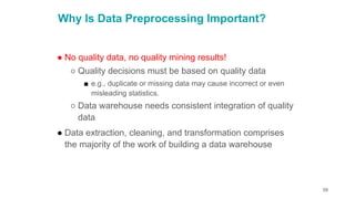
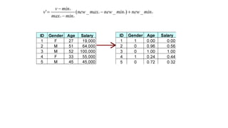
117. Data Transformation: Normalization
●Min-max normalization: to [new_minA
, new_maxA
]
○ Ex. Let income range $12,000 to $98,000 normalized to [0.0, 1.0]. Then
$73,600 is mapped to

119. Data Transformation: Normalization
●Z-score normalization (μ: mean, σ: standard deviation): (zero-mean
normalization)
○
○ Ex. Let μ = 54,000, σ = 16,000. Then $73,600 is mapped to

120. Mean = 80.3
Stdev = 9.84

121. Data Preprocessing
●Why preprocess the data?
●Data cleaning
●Data integration and transformation
●Data reduction
●Descriptive data summarization
●(Descriptive Statistical Measures )

122. Data Reduction Strategies
●Why data reduction?
○ A database/data warehouse may store terabytes of data
○ Complex data analysis/mining may take a very long time to run
on the complete data set
●Data reduction
○ Obtain a reduced representation of the data set that is much
smaller in volume but yet produce the same (or almost the same)
analytical results
●Data reduction strategies
1. Attribute subset selection
2. Dimensionality reduction — e.g., remove unimportant attributes
Data Compression

123. 1. Attribute Subset Selection
● Feature selection (i.e., attribute subset selection):
▪ Attribute subset selection reduces the data set size by
removing irrelevant or redundant attributes (or dimensions).
▪ The goal of attribute subset selection is to find a minimum
set of attributes such that the resulting probability distribution
of the data classes is as close as possible to the original
distribution obtained using all attributes.
▪ How can we find a ‘good’ subset of the original attributes?
1. For n attributes, there are 2n
possible subsets
An exhaustive search(Generate-Test) for the optimal subset of
attributes can be prohibitively expensive, especially as n and
the number of data classes increase.

124. 1. Attribute Subset Selection
●Heuristic methods that explore a reduced search
space are commonly used for attribute subset
selection.
●Heuristic methods (due to exponential # of choices):
○ Step-wise forward selection
○ Step-wise backward elimination
○ Combining forward selection and backward elimination
○ Decision-tree induction