Discrete Time Signal Processing 3rd Edition Alan V. Oppenheim
Discrete Time Signal Processing 3rd Edition Alan V. Oppenheim
Discrete Time Signal Processing 3rd Edition Alan V. Oppenheim
Discrete Time Signal Processing 3rd Edition Alan V. Oppenheim
Discrete Time Signal Processing 3rd Edition Alan V. Oppenheim
1.
Discrete Time SignalProcessing 3rd Edition Alan
V. Oppenheim pdf download
https://ebookname.com/product/discrete-time-signal-
processing-3rd-edition-alan-v-oppenheim/
Get Instant Ebook Downloads – Browse at https://ebookname.com
2.
Instant digital products(PDF, ePub, MOBI) available
Download now and explore formats that suit you...
Discrete systems and digital signal processing with
MATLAB Second Edition Elali
https://ebookname.com/product/discrete-systems-and-digital-
signal-processing-with-matlab-second-edition-elali/
Discrete Random Signal Processing and Filtering Primer
with MATLAB 1st Edition Alexander D. Poularikas
https://ebookname.com/product/discrete-random-signal-processing-
and-filtering-primer-with-matlab-1st-edition-alexander-d-
poularikas/
Digital Signal Processing A Practitioner s Approach 1st
Edition Kaluri V. Rangarao
https://ebookname.com/product/digital-signal-processing-a-
practitioner-s-approach-1st-edition-kaluri-v-rangarao/
Sleisenger and Fordtran s Gastrointestinal and Liver
Disease Review and Assessment Expert Consult Online and
Print 9e 9th Edition Anthony J. Dimarino Md
https://ebookname.com/product/sleisenger-and-fordtran-s-
gastrointestinal-and-liver-disease-review-and-assessment-expert-
consult-online-and-print-9e-9th-edition-anthony-j-dimarino-md/
3.
Solaris 9 AdministrationA Beginner s Guide 1st Edition
Paul Watters
https://ebookname.com/product/solaris-9-administration-a-
beginner-s-guide-1st-edition-paul-watters/
Beyond Hyperbolicity 1st Edition Mark Hagen
https://ebookname.com/product/beyond-hyperbolicity-1st-edition-
mark-hagen/
Industrial brazing practice 2nd Edition Philip Roberts
https://ebookname.com/product/industrial-brazing-practice-2nd-
edition-philip-roberts/
Bovine Medicine Diseases and Husbandry of Cattle 2nd
Edition A. H. Andrews
https://ebookname.com/product/bovine-medicine-diseases-and-
husbandry-of-cattle-2nd-edition-a-h-andrews/
Constitutional and Administrative Law 4th Edition
Hilaire Barnett
https://ebookname.com/product/constitutional-and-administrative-
law-4th-edition-hilaire-barnett/
4.
Comandante Che GuerrillaSoldier Commander and
Strategist 1956 1967 Paul J. Dosal
https://ebookname.com/product/comandante-che-guerrilla-soldier-
commander-and-strategist-1956-1967-paul-j-dosal/
Contents
Alan V. Oppenheim/RonaldW. Schafer 1025
Alan V. Oppenheim/Ronald W. Schafer 985
Appendix: Random Signals
12. Discrete Hilbert Transforms
Alan V. Oppenheim/Ronald W. Schafer 931
11. Parametric Signal Modeling
Alan V. Oppenheim/Ronald W. Schafer 827
10. Fourier Analysis of Signals Using the Discrete Fourier Transform
Alan V. Oppenheim/Ronald W. Schafer 747
9. Computation of the Discrete Fourier Transform
Alan V. Oppenheim/Ronald W. Schafer 651
8. The Discrete Fourier Transform
Alan V. Oppenheim/Ronald W. Schafer 517
7. Filter Design Techniques
Alan V. Oppenheim/Ronald W. Schafer 391
6. Structures for Discrete-Time Systems
Alan V. Oppenheim/Ronald W. Schafer 287
5. Transform Analysis of Linear Time-Invariant Systems
Alan V. Oppenheim/Ronald W. Schafer 163
4. Sampling of Continuous-Time Signals
Alan V. Oppenheim/Ronald W. Schafer 105
3. The z-Transform
Alan V. Oppenheim/Ronald W. Schafer 11
2. Discrete-Time Signals and Systems
Alan V. Oppenheim/Ronald W. Schafer 1
1. Introduction
Index 1047
Alan V. Oppenheim/Ronald W. Schafer 1039
Appendix: Continuous-Time Filters
8.
Introduction
The rich historyand future promise of signal processing derive from a strong synergy
between increasingly sophisticated applications,new theoretical developments and con-
stantly emerging new hardware architectures and platforms. Signal processing applica-
tions span an immense set of disciplines that include entertainment, communications,
space exploration,medicine,archaeology,geophysics,just to name a few. Signal process-
ing algorithms and hardware are prevalent in a wide range of systems, from highly spe-
cialized military systems and industrial applications to low-cost, high-volume consumer
electronics. Although we routinely take for granted the extraordinary performance of
multimedia systems, such as high definition video, high fidelity audio, and interactive
games, these systems have always relied heavily on state-of-the-art signal processing.
Sophisticated digital signal processors are at the core of all modern cell phones. MPEG
audio and video and JPEG1 image data compression standards rely heavily on signal
processing principles and techniques. High-density data storage devices and new solid-
state memories rely increasingly on the use of signal processing to provide consistency
and robustness to otherwise fragile technologies. As we look to the future, it is clear
that the role of signal processing is expanding, driven in part by the convergence of
communications, computers, and signal processing in both the consumer arena and in
advanced industrial and government applications.
The growing number of applications and demand for increasingly sophisticated
algorithms go hand-in-hand with the rapid development of device technology for imple-
menting signal processing systems. By some estimates, even with impending limitations
1The acronyms MPEG and JPEG are the terms used in even casual conversation for referring to the
standards developed by the “Moving Picture Expert Group (MPEG)” and the “Joint Photographic Expert
Group (JPEG)” of the “International Organization for Standardization (ISO).”
1
9.
Introduction
on Moore’s Law,the processing capability of both special-purpose signal processing
microprocessors and personal computers is likely to increase by several orders of mag-
nitude over the next 10 years. Clearly, the importance and role of signal processing will
continue to expand at an accelerating rate well into the future.
Signal processing deals with the representation,transformation,and manipulation
of signals and the information the signals contain. For example, we may wish to sepa-
rate two or more signals that have been combined by some operation, such as addition,
multiplication, or convolution, or we may want to enhance some signal component or
estimate some parameter of a signal model. In communications systems, it is generally
necessary to do preprocessing such as modulation,signal conditioning,and compression
prior to transmission over a communications channel, and then to carry out postpro-
cessing at the receiver to recover a facsimile of the original signal. Prior to the 1960s,
the technology for such signal processing was almost exclusively continuous-time ana-
log technology.2 A continual and major shift to digital technologies has resulted from
the rapid evolution of digital computers and microprocessors and low-cost chips for
analog to digital (A/D) and digital to analog (D/A) conversion. These developments
in technology have been reinforced by many important theoretical developments, such
as the fast Fourier transform (FFT) algorithm, parametric signal modeling, multirate
techniques,polyphase filter implementation,and new ways of representing signals,such
as with wavelet expansions. As just one example of this shift, analog radio communica-
tion systems are evolving into reconfigurable “software radios” that are implemented
almost exclusively with digital computation.
Discrete-time signal processing is based on processing of numeric sequences in-
dexed on integer variables rather than functions of a continuous independent vari-
able. In digital signal processing (DSP), signals are represented by sequences of finite-
precision numbers, and processing is implemented using digital computation. The more
general term discrete-time signal processing includes digital signal processing as a spe-
cial case but also includes the possibility that sequences of samples (sampled data)
could be processed with other discrete-time technologies. Often the distinction be-
tween the terms discrete-time signal processing and digital signal processing is of minor
importance, since both are concerned with discrete-time signals. This is particularly
true when high-precision computation is employed.Although there are many examples
in which signals to be processed are inherently discrete-time sequences, most applica-
tions involve the use of discrete-time technology for processing signals that originate
as continuous-time signals. In this case, a continuous-time signal is typically converted
into a sequence of samples, i.e., a discrete-time signal. Indeed, one of the most impor-
tant spurs to widespread application of digital signal processing was the development
of low-cost A/D, D/A conversion chips based on differential quantization with noise
shaping. After discrete-time processing, the output sequence is converted back to a
continuous-time signal. Real-time operation is often required or desirable for such sys-
tems. As computer speeds have increased, discrete-time processing of continuous-time
signals in real time has become commonplace in communication systems, radar and
sonar, speech and video coding and enhancement, biomedical engineering, and many
2In a general context, we shall refer to the independent variable as “time,” even though in specific
contexts, the independent variable may take on any of a broad range of possible dimensions. Consequently,
continuous time and discrete time should be thought of as generic terms referring to a continuous independent
variable and a discrete independent variable, respectively.
2
10.
Introduction
other areas ofapplication. Non-real-time applications are also common. The compact
disc player and MP3 player are examples of asymmetric systems in which an input signal
is processed only once. The initial processing may occur in real time, slower than real
time, or even faster than real time. The processed form of the input is stored (on the
compact disc or in a solid state memory), and final processing for reconstructing the
audio signal is carried out in real time when the output is played back for listening. The
compact disc and MP3 recording and playback systems rely on many signal processing
concepts.
Financial Engineering represents another rapidly emerging field which incorpo-
rates many signal processing concepts and techniques. Effective modeling, prediction
and filtering of economic data can result in significant gains in economic performance
and stability. Portfolio investment managers, for example, are relying increasingly on
using sophisticated signal processing since even a very small increase in signal pre-
dictability or signal-to-noise ratio (SNR) can result in significant gain in performance.
Another important area of signal processing is signal interpretation. In such con-
texts, the objective of the processing is to obtain a characterization of the input signal.
For example, in a speech recognition or understanding system, the objective is to in-
terpret the input signal or extract information from it. Typically, such a system will
apply digital pre-processing (filtering, parameter estimation, and so on) followed by a
pattern recognition system to produce a symbolic representation, such as a phonemic
transcription of the speech. This symbolic output can, in turn, be the input to a sym-
bolic processing system, such as a rules-based expert system, to provide the final signal
interpretation.
Still another relatively new category of signal processing involves the symbolic
manipulation of signal processing expressions. This type of processing is potentially
useful in signal processing workstations and for the computer-aided design of signal
processing systems. In this class of processing, signals and systems are represented and
manipulated as abstract data objects. Object-oriented programming languages provide
a convenient environment for manipulating signals, systems, and signal processing ex-
pressions without explicitly evaluating the data sequences.The sophistication of systems
designed to do signal expression processing is directly influenced by the incorporation
of fundamental signal processing concepts, theorems, and properties, such as those that
form the basis for this book. For example, a signal processing environment that incor-
porates the property that convolution in the time domain corresponds to multiplication
in the frequency domain can explore a variety of rearrangements of filtering structures,
including those involving the direct use of the discrete Fourier transform (DFT) and the
FFT algorithm. Similarly,environments that incorporate the relationship between sam-
pling rate and aliasing can make effective use of decimation and interpolation strategies
for filter implementation. Similar ideas are currently being explored for implementing
signal processing in network environments. In this type of environment, data can po-
tentially be tagged with a high-level description of the processing to be done, and the
details of the implementation can be based dynamically on the resources available on
the network.
Many concepts and design techniques are now incorporated into the structure
of sophisticated software systems such as MATLAB, Simulink, Mathematica, and Lab-
VIEW. In many cases where discrete-time signals are acquired and stored in computers,
these tools allow extremely sophisticated signal processing operations to be formed
3
11.
Introduction
from basic functions.In such cases, it is not generally necessary to know the details
of the underlying algorithm that implements the computation of an operation like the
FFT, but nevertheless it is essential to understand what is computed and how it should
be interpreted. In other words, a good understanding of the concepts considered in this
text is essential for intelligent use of the signal processing software tools that are now
widely available.
Signal processing problems are not confined,of course,to one-dimensional signals.
Although there are some fundamental differences in the theories for one-dimensional
and multidimensional signal processing, much of the material that we discuss in this
text has a direct counterpart in multidimensional systems. The theory of multidimen-
sional digital signal processing is presented in detail in a variety of references including
Dudgeon and Mersereau (1984), Lim (1989), and Bracewell (1994).3 Many image pro-
cessing applications require the use of two-dimensional signal processing techniques.
This is the case in such areas as video coding, medical imaging, enhancement and analy-
sis of aerial photographs,analysis of satellite weather photos,and enhancement of video
transmissions from lunar and deep-space probes.Applications of multidimensional dig-
ital signal processing to image processing are discussed,for example,in Macovski (1983),
Castleman (1996), Jain (1989), Bovic (ed.) (2005),Woods (2006), Gonzalez and Woods
(2007),and Pratt (2007). Seismic data analysis as required in oil exploration,earthquake
measurement, and nuclear test monitoring also uses multidimensional signal process-
ing techniques. Seismic applications are discussed in, for example, Robinson and Treitel
(1980) and Robinson and Durrani (1985).
Multidimensional signal processing is only one of many advanced and specialized
topics that build on signal-processing fundamentals. Spectral analysis based on the use
of the DFT and the use of signal modeling is another particularly rich and important
aspect of signal processing. High resolution spectrum analysis methods also are based
on representing the signal to be analyzed as the response of a discrete-time linear time-
invariant (LTI) filter to either an impulse or to white noise. Spectral analysis is achieved
by estimating the parameters (e.g., the difference equation coefficients) of the system
and then evaluating the magnitude squared of the frequency response of the model
filter. Detailed discussions of spectrum analysis can be found in the texts by Kay (1988),
Marple (1987),Therrien (1992), Hayes (1996) and Stoica and Moses (2005).
Signal modeling also plays an important role in data compression and coding,
and here again, the fundamentals of difference equations provide the basis for under-
standing many of these techniques. For example, one class of signal coding techniques,
referred to as linear predictive coding (LPC), exploits the notion that if a signal is the
response of a certain class of discrete-time filters, the signal value at any time index is a
linear function of (and thus linearly predictable from) previous values. Consequently,
efficient signal representations can be obtained by estimating these prediction param-
eters and using them along with the prediction error to represent the signal. The signal
can then be regenerated when needed from the model parameters. This class of signal
3Authors names and dates are used to refer to books and papers listed in the Bibliography at the end
of this chapter.
4
12.
Introduction
coding techniques hasbeen particularly effective in speech coding and is described in
considerable detail in Jayant and Noll (1984), Markel and Gray (1976), Rabiner and
Schafer (1978) and Quatieri (2002).
Another advanced topic of considerable importance is adaptive signal processing.
Adaptive systems represent a particular class of time-varying and, in some sense, non-
linear systems with broad application and with established and effective techniques for
their design and analysis. Again, many of these techniques build from the fundamentals
of discrete-time signal processing. Details of adaptive signal processing are given by
Widrow and Stearns (1985), Haykin (2002) and Sayed (2008).
These represent only a few of the many advanced topics that extend from the
content covered in this text. Others include advanced and specialized filter design pro-
cedures,a variety of specialized algorithms for evaluation of the Fourier transform,spe-
cialized filter structures, and various advanced multirate signal processing techniques,
including wavelet transforms. (See Burrus, Gopinath, and Guo (1997), Vaidyanathan
(1993) and Vetterli and Kovačević (1995) for introductions to these topics.)
It has often been said that the purpose of a fundamental textbook should be to
uncover, rather than cover, a subject. We have been guided by this philosophy. There is
a rich variety of both challenging theory and compelling applications to be uncovered
by those who diligently prepare themselves with a study of the fundamentals of DSP.
HISTORIC PERSPECTIVE
Discrete-time signal processing has advanced in uneven steps over time. Looking back
at the development of the field of discrete-time signal processing provides a valuable
perspective on fundamentals that will remain central to the field for a long time to
come. Since the invention of calculus in the 17th century, scientists and engineers have
developed models to represent physical phenomena in terms of functions of continuous
variables and differential equations. However, numeric techniques have been used to
solve these equations when analytical solutions are not possible. Indeed, Newton used
finite-difference methods that are special cases of some of the discrete-time systems that
we present in this text. Mathematicians of the 18th century,such as Euler,Bernoulli,and
Lagrange,developed methods for numeric integration and interpolation of functions of
a continuous variable. Interesting historic research by Heideman, Johnson, and Burrus
(1984) showed that Gauss discovered the fundamental principle of the FFT as early as
1805—even before the publication of Fourier’s treatise on harmonic series representa-
tion of functions.
Until the early 1950s, signal processing as we have defined it was typically carried
out with analog systems implemented with electronic circuits or even with mechanical
devices. Even though digital computers were becoming available in business environ-
ments and in scientific laboratories, they were expensive and had relatively limited
capabilities. About that time, the need for more sophisticated signal processing in some
application areas created considerable interest in discrete-time signal processing. One
of the first uses of digital computers in DSP was in geophysical exploration, where rel-
atively low frequency seismic signals could be digitized and recorded on magnetic tape
5
13.
Introduction
for later processing.This type of signal processing could not generally be done in real
time; minutes or even hours of computer time were often required to process only
seconds of data. Even so,the flexibility of the digital computer and the potential payoffs
made this alternative extremely inviting.
Also in the 1950s, the use of digital computers in signal processing arose in a
different way. Because of the flexibility of digital computers, it was often useful to sim-
ulate a signal processing system on a digital computer before implementing it in analog
hardware. In this way, a new signal processing algorithm or system could be studied
in a flexible experimental environment before committing economic and engineering
resources to constructing it.Typical examples of such simulations were the vocoder sim-
ulations carried out at Massachusetts Institute ofTechnology (MIT) Lincoln Laboratory
and Bell Telephone Laboratories. In the implementation of an analog channel vocoder,
for example, the filter characteristics affected the perceived quality of the coded speech
signal in ways that were difficult to quantify objectively. Through computer simulations,
these filter characteristics could be adjusted and the perceived quality of a speech coding
system evaluated prior to construction of the analog equipment.
In all of these examples of signal processing using digital computers,the computer
offered tremendous advantages in flexibility. However,the processing could not be done
in real time. Consequently, the prevalent attitude up to the late 1960s was that the dig-
ital computer was being used to approximate, or simulate, an analog signal processing
system. In keeping with that style, early work on digital filtering concentrated on ways
in which a filter could be programmed on a digital computer so that with A/D conver-
sion of the signal, followed by digital filtering, followed by D/A conversion, the overall
system approximated a good analog filter. The notion that digital systems might, in fact,
be practical for the actual real-time implementation of signal processing in speech com-
munication, radar processing, or any of a variety of other applications seemed, even at
the most optimistic times, to be highly speculative. Speed, cost, and size were, of course,
three of the important factors in favor of the use of analog components.
As signals were being processed on digital computers, researchers had a natural
tendency to experiment with increasingly sophisticated signal processing algorithms.
Some of these algorithms grew out of the flexibility of the digital computer and had no
apparent practical implementation in analog equipment.Thus,many of these algorithms
were treated as interesting,but somewhat impractical,ideas. However,the development
of such signal processing algorithms made the notion of all-digital implementation of
signal processing systems even more tempting. Active work began on the investigation
of digital vocoders, digital spectrum analyzers, and other all-digital systems, with the
hope that eventually, such systems would become practical.
The evolution of a new point of view toward discrete-time signal processing was
further accelerated by the disclosure by Cooley and Tukey (1965) of an efficient class
of algorithms for computation of Fourier transforms known collectively as the FFT.
The FFT was significant for several reasons. Many signal processing algorithms that
had been developed on digital computers required processing times several orders of
magnitude greater than real time. Often, this was because spectrum analysis was an
important component of the signal processing and no efficient means were available for
implementing it. The FFT reduced the computation time of the Fourier transform by
orders of magnitude,permitting the implementation of increasingly sophisticated signal
6
14.
Introduction
processing algorithms withprocessing times that allowed interactive experimentation
with the system. Furthermore, with the realization that the FFT algorithms might, in
fact, be implementable with special-purpose digital hardware, many signal processing
algorithms that previously had appeared to be impractical began to appear feasible.
Another important implication of the FFT was that it was an inherently discrete-
time concept. It was directed toward the computation of the Fourier transform of a
discrete-time signal or sequence and involved a set of properties and mathematics
that was exact in the discrete-time domain—it was not simply an approximation to
a continuous-time Fourier transform. This had the effect of stimulating a reformulation
of many signal processing concepts and algorithms in terms of discrete-time mathemat-
ics, and these techniques then formed an exact set of relationships in the discrete-time
domain. Following this shift away from the notion that signal processing on a digital
computer was merely an approximation to analog signal processing techniques, there
emerged the current view that discrete-time signal processing is an important field of
investigation in its own right.
Another major development in the history of discrete-time signal processing oc-
curred in the field of microelectronics. The invention and subsequent proliferation of
the microprocessor paved the way for low-cost implementations of discrete-time signal
processing systems.Although the first microprocessors were too slow to implement most
discrete-time systems in real time except at very low sampling rates, by the mid-1980s,
integrated circuit technology had advanced to a level that permitted the implementation
of very fast fixed-point and floating-point microcomputers with architectures specially
designed for implementing discrete-time signal processing algorithms. With this tech-
nology came,for the first time,the possibility of widespread application of discrete-time
signal processing techniques. The rapid pace of development in microelectronics also
significantly impacted the development of signal processing algorithms in other ways.
For example, in the early days of real-time digital signal processing devices, memory
was relatively costly and one of the important metrics in developing signal processing
algorithms was the efficient use of memory. Digital memory is now so inexpensive that
many algorithms purposely incorporate more memory than is absolutely required so
that the power requirements of the processor are reduced. Another area in which tech-
nology limitations posed a significant barrier to widespread deployment of DSP was in
conversion of signals from analog to discrete-time (digital) form. The first widely avail-
ableA/D and D/A converters were stand-alone devices costing thousands of dollars. By
combining digital signal processing theory with microelectronic technology, oversam-
pled A/D and D/A converters costing a few dollars or less have enabled a myriad of
real-time applications.
In a similar way, minimizing the number of arithmetic operations, such as multi-
plies or floating point additions, is now less essential, since multicore processors often
have several multipliers available and it becomes increasingly important to reduce com-
munication between cores, even if it then requires more multiplications. In a multicore
environment,for example,direct computation of the DFT (or the use of the Goertzel al-
gorithm) is more“efficient”than the use of an FFT algorithm since,although many more
multiplications are required,communication requirements are significantly reduced be-
cause the processing can be more efficiently distributed among multiple processors or
cores. More broadly, the restructuring of algorithms and the development of new ones
7
15.
Introduction
to exploit theopportunity for more parallel and distributed processing is becoming a
significant new direction in the development of signal processing algorithms.
FUTURE PROMISE
Microelectronics engineers continue to strive for increased circuit densities and produc-
tion yields,and as a result,the complexity and sophistication of microelectronic systems
continually increase. The complexity, speed, and capability of DSP chips have grown
exponentially since the early 1980s and show no sign of slowing down. As wafer-scale
integration techniques become highly developed, very complex discrete-time signal
processing systems will be implemented with low cost, miniature size, and low power
consumption. Furthermore, technologies such as microelectronic mechanical systems
(MEMS) promise to produce many types of tiny sensors whose outputs will need to
be processed using DSP techniques that operate on distributed arrays of sensor inputs.
Consequently, the importance of discrete-time signal processing will continue to in-
crease,and the future development of the field promises to be even more dramatic than
the course of development that we have just described.
Discrete-time signal processing techniques have already promoted revolutionary
advances in some fields of application.A notable example is in the area of telecommuni-
cations, where discrete-time signal processing techniques, microelectronic technology,
and fiber optic transmission have combined to change the nature of communication
systems in truly revolutionary ways. A similar impact can be expected in many other
areas. Indeed, signal processing has always been, and will always be, a field that thrives
on new applications. The needs of a new field of application can sometimes be filled
by knowledge adapted from other applications, but frequently, new application needs
stimulate new algorithms and new hardware systems to implement those algorithms.
Early on,applications to seismology,radar,and communication provided the context for
developing many of the core signal processing techniques. Certainly, signal processing
will remain at the heart of applications in national defense, entertainment, communi-
cation, and medical care and diagnosis. Recently, we have seen applications of signal
processing techniques in new areas as disparate as finance and DNA sequence analysis.
Although it is difficult to predict where other new applications will arise, there is
no doubt that they will be obvious to those who are prepared to recognize them. The
key to being ready to solve new signal processing problems is, and has always been,
a thorough grounding in the fundamental mathematics of signals and systems and in
the associated design and processing algorithms. While discrete-time signal processing
is a dynamic, steadily growing field, its fundamentals are well formulated, and it is ex-
tremely valuable to learn them well. Our goal is to uncover the fundamentals of the
field by providing a coherent treatment of the theory of discrete-time linear systems,
filtering, sampling, discrete-time Fourier analysis, and signal modeling. We hope to pro-
vide the reader with the knowledge necessary for an appreciation of the wide scope
of applications for discrete-time signal processing and a foundation for contributing to
future developments in this exciting field.
8
16.
Introduction
BIBLIOGRAPHY
Bovic, A., ed.,Handbook of Image and Video Processing, 2nd ed., Academic Press, Burlington,
MA, 2005.
Bracewell, R. N.,Two-Dimensional Imaging, Prentice Hall, New York, NY, 1994.
Burrus, C. S., Gopinath, R. A., and Guo, H., Introduction to Wavelets and Wavelet Transforms: A
Primer, Prentice Hall, 1997.
Castleman, K. R., Digital Image Processing, 2nd ed., Prentice Hall, Upper Saddle River, NJ, 1996.
Cooley, J. W., and Tukey, J. W.,“An Algorithm for the Machine Computation of Complex Fourier
Series,” Mathematics of Computation,Vol. 19, pp. 297–301,Apr. 1965.
Dudgeon,D. E.,and Mersereau,R. M.,Two-Dimensional Digital Signal Processing,Prentice Hall,
Englewood Cliffs, NJ, 1984.
Gonzalez, R. C., and Woods, R. E., Digital Image Processing,Wiley, 2007.
Hayes, M., Statistical Digital Signal Processing and Modeling,Wiley, New York, NY, 1996.
Haykin, S.,Adaptive Filter Theory, 4th ed., Prentice Hall, 2002.
Heideman, M. T., Johnson, D. H., and Burrus, C. S., “Gauss and the History of the Fast Fourier
Transform,” IEEE ASSP Magazine,Vol. 1, No. 4, pp. 14–21, Oct. 1984.
Jain,A. K., Fundamentals of Digital Image Processing, Prentice Hall, Englewood Cliffs, NJ, 1989.
Jayant, N. S., and Noll, P., Digital Coding of Waveforms, Prentice Hall, Englewood Cliffs, NJ, 1984.
Kay, S. M., Modern Spectral Estimation Theory and Application, Prentice Hall, Englewood Cliffs,
NJ, 1988.
Lim, J. S.,Two-Dimensional Digital Signal Processing, Prentice Hall, Englewood Cliffs, NJ, 1989.
Macovski,A., Medical Image Processing, Prentice Hall, Englewood Cliffs, NJ, 1983.
Markel, J. D., and Gray, A. H., Jr., Linear Prediction of Speech, Springer-Verlag, New York, NY,
1976.
Marple, S. L., Digital Spectral Analysis with Applications, Prentice Hall, Englewood Cliffs, NJ,
1987.
Pratt,W., Digital Image Processing, 4th ed.,Wiley, New York, NY, 2007.
Quatieri, T. F., Discrete-Time Speech Signal Processing: Principles and Practice, Prentice Hall,
Englewood Cliffs, NJ, 2002.
Rabiner,L. R.,and Schafer,R.W.,Digital Processing of Speech Signals,Prentice Hall,Englewood
Cliffs, NJ, 1978.
Robinson, E. A., and Durrani, T. S., Geophysical Signal Processing, Prentice Hall, Englewood
Cliffs, NJ, 1985.
Robinson, E. A., and Treitel, S., Geophysical Signal Analysis, Prentice Hall, Englewood Cliffs, NJ,
1980.
Sayed,A.,Adaptive Filters,Wiley, Hoboken, NJ, 2008.
Stoica, P., and Moses, R., Spectral Analysis of Signals, Pearson Prentice Hall, Upper Saddle River,
NJ, 2005.
Therrien, C. W., Discrete Random Signals and Statistical Signal Processing, Prentice Hall, Engle-
wood Cliffs, NJ, 1992.
Vaidyanathan, P. P., Multirate Systems and Filter Banks, Prentice Hall, Englewood Cliffs, NJ, 1993.
Vetterli, M., and Kovačević, J., Wavelets and Subband Coding, Prentice Hall, Englewood Cliffs,
NJ, 1995.
Widrow, B., and Stearns, S. D., Adaptive Signal Processing, Prentice Hall, Englewood Cliffs, NJ,
1985.
Woods, J. W., Multidimensional Signal, Image, and Video Processing and Coding,Academic Press,
2006.
9
17.
Discrete-Time
Signals and Systems
0INTRODUCTION
The independent variable in the mathematical representation of a signal may be
either continuous or discrete. Continuous-time signals are defined along a continuum of
time and are thus represented by a continuous independent variable. Continuous-time
signalsareoftenreferredtoasanalogsignals.Discrete-timesignalsaredefinedatdiscrete
times,and thus,the independent variable has discrete values;that is,discrete-time signals
are represented as sequences of numbers. Signals such as speech or images may have
either a continuous- or a discrete-variable representation,and if certain conditions hold,
these representations are entirely equivalent. Besides the independent variables being
either continuous or discrete,the signal amplitude may be either continuous or discrete.
Digital signals are those for which both time and amplitude are discrete.
The term signal is generally applied to something that conveys information. Signals may,
for example, convey information about the state or behavior of a physical system. As
another class of examples, signals are synthesized for the purpose of communicating
information between humans or between humans and machines. Although signals can
be represented in many ways, in all cases, the information is contained in some pat-
tern of variations. Signals are represented mathematically as functions of one or more
independent variables. For example, a speech signal is represented mathematically as
a function of time, and a photographic image is represented as a brightness function of
two spatial variables. A common convention is to refer to the independent variable of
the mathematical representation of a signal as time, although in specific examples, the
independent variable may not in fact correspond to time.
18.
Discrete-Time Signals andSystems
Signal-processing systems may be classified along the same lines as signals. That
is, continuous-time systems are systems for which both the input and the output are
continuous-time signals, and discrete-time systems are those for which both the input
and the output are discrete-time signals. Similarly, a digital system is a system for which
both the input and the output are digital signals. Digital signal processing, then, deals
with the transformation of signals that are discrete in both amplitude and time. The
principalfocusofthisbookisondiscrete-time—ratherthandigital—signalsandsystems.
However, the theory of discrete-time signals and systems is also exceedingly useful for
digital signals and systems, particularly if the signal amplitudes are finely quantized.
In this chapter, we present the basic definitions, establish notation, and develop
and review the basic concepts associated with discrete-time signals and systems. The
presentation of this material assumes that the reader has had previous exposure to some
of this material, perhaps with a different emphasis and notation. Thus, this chapter is
primarily intended to provide a common foundation for more advanced material.
In Section 1, we discuss the representation of discrete-time signals as sequences
and describe the basic sequences such as the unit impulse, the unit step, and com-
plex exponential, which play a central role in characterizing discrete-time systems and
form building blocks for more general sequences. In Section 2,the representation,basic
properties, and simple examples of discrete-time systems are presented. Sections 3 and
4 focus on the important class of linear time-invariant (LTI) systems and their time-
domain representation through the convolution sum, with Section 5 considering the
specific class of LTI systems represented by linear,constant–coefficient difference equa-
tions. Section 6 develops the frequency domain representation of discrete-time systems
through the concept of complex exponentials as eigenfunctions, and Sections 7, 8, and 9
develop and explore the Fourier transform representation of discrete-time signals as a
linear combination of complex exponentials. Section 10 provides a brief introduction
to discrete-time random signals.
1 DISCRETE-TIME SIGNALS
Discrete-time signals are represented mathematically as sequences of numbers.
A sequence of numbers x, in which the nth number in the sequence is denoted x[n],1 is
formally written as
x = {x[n]}, −∞ < n < ∞, (1)
where n is an integer. In a practical setting,such sequences can often arise from periodic
sampling of an analog (i.e.,continuous-time) signal xa(t). In that case,the numeric value
of the nth number in the sequence is equal to the value of the analog signal, xa(t), at
time nT: i.e.,
x[n] = xa(nT ), −∞ < n < ∞. (2)
The quantity T is the sampling period, and its reciprocal is the sampling frequency.
Although sequences do not always arise from sampling analog waveforms, it is con-
venient to refer to x[n] as the “nth sample” of the sequence. Also, although, strictly
1Note that we use [ ] to enclose the independent variable of discrete-variable functions, and we use ( )
to enclose the independent variable of continuous-variable functions.
12
19.
Discrete-Time Signals andSystems
speaking, x[n] denotes the nth number in the sequence, the notation of Eq. (1) is of-
ten unnecessarily cumbersome, and it is convenient and unambiguous to refer to “the
sequence x[n]” when we mean the entire sequence, just as we referred to “the analog
signal xa(t).” We depict discrete-time signals (i.e., sequences) graphically, as shown in
Figure 1.Although the abscissa is drawn as a continuous line,it is important to recognize
that x[n] is defined only for integer values of n. It is not correct to think of x[n] as being
zero when n is not an integer; x[n] is simply undefined for noninteger values of n.
–9 –7 –5 –3
–4
–6
–8 0 1 2 3 4 5 6
7 8 9 10 11
–1
–2
x[0]
x[1]
x[2]
x[n]
x[–1]
x[–2]
n Figure 1 Graphic representation of a
discrete-time signal.
As an example of a sequence obtained by sampling, Figure 2(a) shows a segment
of a speech signal corresponding to acoustic pressure variation as a function of time,and
Figure 2(b) presents a sequence of samples of the speech signal. Although the original
speech signal is defined at all values of time t, the sequence contains information about
the signal only at discrete instants. The sampling theorem guarantees that the original
32 ms
(a)
256 samples
(b)
Figure 2 (a) Segment of a continuous-time speech signal xa(t ). (b) Sequence of samples
x[n] = xa(nT ) obtained from the signal in part (a) with T = 125 μs.
13
20.
Discrete-Time Signals andSystems
signal can be reconstructed as accurately as desired from a corresponding sequence of
samples if the samples are taken frequently enough.
In discussing the theory of discrete-time signals and systems, several basic se-
quences are of particular importance. These sequences are shown in Figure 3 and will
be discussed next.
The unit sample sequence (Figure 3a) is defined as the sequence
δ[n] =
0, n = 0,
1, n = 0.
(3)
The unit sample sequence plays the same role for discrete-time signals and systems that
the unit impulse function (Dirac delta function) does for continuous-time signals and
systems. For convenience, we often refer to the unit sample sequence as a discrete-time
impulse or simply as an impulse. It is important to note that a discrete-time impulse
does not suffer from the mathematic complications of the continuous-time impulse; its
definition in Eq. (3) is simple and precise.
1
Unit sample
0
(a)
n
1
Unit step
0
(b)
...
...
...
...
n
Real exponential
0
(c)
n
Sinusoidal
0
(d)
...
...
...
...
n
Figure 3 Some basic sequences. The
sequences shown play important roles
in the analysis and representation of
discrete-time signals and systems.
14
21.
Discrete-Time Signals andSystems
1
0 3 4 5 6 8
7
2
–2
–4
p[n]
n
a–3
a1
a2
a7
Figure 4 Example of a sequence to be
represented as a sum of scaled, delayed
impulses.
One of the important aspects of the impulse sequence is that an arbitrary sequence
can be represented as a sum of scaled,delayed impulses. For example,the sequence p[n]
in Figure 4 can be expressed as
p[n] = a−3δ[n + 3] + a1δ[n − 1] + a2δ[n − 2] + a7δ[n − 7]. (4)
More generally, any sequence can be expressed as
x[n] =
∞
k=−∞
x[k]δ[n − k]. (5)
We will make specific use of Eq. (5) in discussing the representation of discrete-time
linear systems.
The unit step sequence (Figure 3b) is defined as
u[n] =
1, n ≥ 0,
0, n 0.
(6)
The unit step is related to the unit impulse by
u[n] =
n
k=−∞
δ[k]; (7)
that is, the value of the unit step sequence at (time) index n is equal to the accumulated
sum of the value at index n and all previous values of the impulse sequence. An alterna-
tive representation of the unit step in terms of the impulse is obtained by interpreting
the unit step in Figure 3(b) in terms of a sum of delayed impulses, as in Eq. (5). In this
case, the nonzero values are all unity, so
u[n] = δ[n] + δ[n − 1] + δ[n − 2] + · · · (8a)
or
u[n] =
∞
k=0
δ[n − k]. (8b)
As yet another alternative, the impulse sequence can be expressed as the first backward
difference of the unit step sequence, i.e.,
δ[n] = u[n] − u[n − 1]. (9)
Exponential sequences are another important class of basic signals. The general
form of an exponential sequence is
x[n] = A αn
. (10)
If A and α are real numbers, then the sequence is real. If 0 α 1 and A is positive,
then the sequence values are positive and decrease with increasing n, as in Figure 3(c).
15
22.
Discrete-Time Signals andSystems
For −1 α 0, the sequence values alternate in sign but again decrease in magnitude
with increasing n. If |α| 1, then the sequence grows in magnitude as n increases.
The exponential sequence A αn with α complex has real and imaginary parts that
are exponentially weighted sinusoids. Specifically, if α = |α|ejω0 and A = |A |ejφ, the
sequence A αn can be expressed in any of the following ways:
x[n] = A αn
= |A |ejφ
|α|n
ejω0n
= |A | |α|n
ej(ω0n+φ)
(11)
= |A | |α|n
cos(ω0n + φ) + j|A | |α|n
sin(ω0n + φ).
The sequence oscillates with an exponentially growing envelope if |α| 1 or with an
exponentially decaying envelope if |α| 1. (As a simple example, consider the case
ω0 = π.)
When |α| = 1, the sequence has the form
x[n] = |A |ej(ω0n+φ)
= |A | cos(ω0n + φ) + j|A | sin(ω0n + φ); (12)
that is,the real and imaginary parts of ejω0n vary sinusoidally with n. By analogy with the
continuous-time case, the quantity ω0 is called the frequency of the complex sinusoid
or complex exponential, and φ is called the phase. However, since n is a dimensionless
integer, the dimension of ω0 is radians. If we wish to maintain a closer analogy with the
continuous-time case, we can specify the units of ω0 to be radians per sample and the
units of n to be samples.
The fact that n is always an integer in Eq. (12) leads to some important differences
between the properties of discrete-time and continuous-time complex exponential se-
quences and sinusoidal sequences. Consider, for example, a frequency (ω0 +2π). In this
case,
x[n] = A ej(ω0+2π)n
= A ejω0nej2πn = A ejω0n.
(13)
Generally, complex exponential sequences with frequencies (ω0 + 2πr), where r is an
integer, are indistinguishable from one another. An identical statement holds for sinu-
soidal sequences. Specifically, it is easily verified that
x[n] = A cos[(ω0 + 2πr)n + φ]
= A cos(ω0n + φ).
(14)
When discussing complex exponential signals of the form x[n] = A ejω0n or real sinu-
soidal signals of the form x[n] = A cos(ω0n + φ), we need only consider frequencies in
an interval of length 2π. Typically, we will choose either −π ω0 ≤ π or 0 ≤ ω0 2π.
Another important difference between continuous-time and discrete-time com-
plex exponentials and sinusoids concerns their periodicity in n. In the continuous-time
case,a sinusoidal signal and a complex exponential signal are both periodic in time with
the period equal to 2π divided by the frequency. In the discrete-time case, a periodic
sequence is a sequence for which
x[n] = x[n + N ], for all n, (15)
16
23.
Discrete-Time Signals andSystems
where the period N is necessarily an integer. If this condition for periodicity is tested
for the discrete-time sinusoid, then
A cos(ω0n + φ) = A cos(ω0n + ω0N + φ), (16)
which requires that
ω0N = 2πk, (17)
where k is an integer. A similar statement holds for the complex exponential sequence
Cejω0n; that is, periodicity with period N requires that
ejω0(n+N)
= ejω0n
, (18)
which is true only for ω0N = 2πk, as in Eq. (17). Consequently, complex exponential
and sinusoidal sequences are not necessarily periodic in n with period (2π/ω0) and,
depending on the value of ω0, may not be periodic at all.
Example 1 Periodic and Aperiodic Discrete-Time Sinusoids
Consider the signal x1[n] = cos(πn/4). This signal has a period of N = 8. To show this,
note that x[n + 8] = cos(π(n + 8)/4) = cos(πn/4 + 2π) = cos(πn/4) = x[n], satisfying
the definition of a discrete-time periodic signal. Contrary to continuous-time sinusoids,
increasing the value of ω0 for a discrete-time sinusoid does not necessarily decrease
the period of the signal. Consider the discrete-time sinusoid x2[n] = cos(3πn/8),which
has a higher frequency than x1[n]. However, x2[n] is not periodic with period 8, since
x2[n + 8] = cos(3π(n + 8)/8) = cos(3πn/8 + 3π) = −x2[n]. Using an argument anal-
ogous to the one for x1[n], we can show that x2[n] has a period of N = 16. Thus,
increasing the value of ω0 = 2π/8 to ω0 = 3π/8 also increases the period of the signal.
This occurs because discrete-time signals are defined only for integer indices n.
The integer restriction on n results in some sinusoidal signals not being periodic
at all. For example, there is no integer N such that the signal x3[n] = cos(n) satisfies
the condition x3[n + N ] = x3[n] for all n. These and other properties of discrete-time
sinusoids that run counter to their continuous-time counterparts are caused by the
limitation of the time index n to integers for discrete-time signals and systems.
When we combine the condition of Eq. (17) with our previous observation that
ω0 and (ω0 + 2πr) are indistinguishable frequencies, it becomes clear that there are N
distinguishable frequencies for which the corresponding sequences are periodic with
period N. One set of frequencies is ωk = 2πk/N, k = 0, 1, . . . , N − 1. These properties
of complex exponential and sinusoidal sequences are basic to both the theory and the
design of computational algorithms for discrete-time Fourier analysis.
Related to the preceding discussion is the fact that the interpretation of high
and low frequencies is somewhat different for continuous-time and discrete-time sinu-
soidal and complex exponential signals. For a continuous-time sinusoidal signal x(t) =
A cos(0t + φ), as 0 increases, x(t) oscillates progressively more rapidly. For the
discrete-time sinusoidal signal x[n] = A cos(ω0n + φ), as ω0 increases from ω0 = 0 to-
ward ω0 = π, x[n] oscillates progressively more rapidly. However, as ω0 increases from
ω0 = π to ω0 = 2π, the oscillations become slower. This is illustrated in Figure 5. In
17
24.
0
(a)
...
...
n
0 = 0or 0 = 2
0
(b)
...
...
n
0 = /8 or 0 = 15/8
0 = /4 or 0 = 7/4
0
(c)
...
...
n
0
(d)
...
...
...
...
n
0 =
Figure 5 cos ω 0n for several different values of ω0. As ω 0 increases from zero
toward π (parts a–d), the sequence oscillates more rapidly. As ω0 increases from
π to 2π (parts d–a), the oscillations become slower.
18
25.
Discrete-Time Signals andSystems
fact, because of the periodicity in ω0 of sinusoidal and complex exponential sequences,
ω0 = 2π is indistinguishable from ω0 = 0, and, more generally, frequencies around
ω0 = 2π are indistinguishable from frequencies around ω0 = 0. As a consequence, for
sinusoidal and complex exponential signals, values of ω0 in the vicinity of ω0 = 2πk
for any integer value of k are typically referred to as low frequencies (relatively slow
oscillations),whereas values of ω0 in the vicinity of ω0 = (π+2πk) for any integer value
of k are typically referred to as high frequencies (relatively rapid oscillations).
2 DISCRETE-TIME SYSTEMS
A discrete-time system is defined mathematically as a transformation or operator that
maps an input sequence with values x[n] into an output sequence with values y[n]. This
can be denoted as
y[n] = T{x[n]} (19)
and is indicated pictorially in Figure 6. Equation (19) represents a rule or formula for
computing the output sequence values from the input sequence values. It should be
emphasized that the value of the output sequence at each value of the index n may
depend on input samples x[n] for all values of n, i.e., y at time n can depend on all or
part of the entire sequence x. The following examples illustrate some simple and useful
systems.
x[n] y[n]
T{•}
Figure 6 Representation of a
discrete-time system, i.e., a
transformation that maps an input
sequence x[n] into a unique output
sequence y[n].
Example 2 The Ideal Delay System
The ideal delay system is defined by the equation
y[n] = x[n − nd], −∞ n ∞, (20)
where nd is a fixed positive integer representing the delay of the system. In other words,
the ideal delay system shifts the input sequence to the right by nd samples to form the
output. If, in Eq. (20), nd is a fixed negative integer, then the system would shift the
input to the left by |nd| samples, corresponding to a time advance.
In the system of Example 2, only one sample of the input sequence is involved in
determining a certain output sample. In the following example, this is not the case.
19
26.
Discrete-Time Signals andSystems
Example 3 Moving Average
The general moving-average system is defined by the equation
y[n] =
1
M1 + M2 + 1
M2
k=−M1
x[n − k]
=
1
M1 + M2 + 1
{x[n + M1] + x[n + M 1 − 1] + · · · + x[n] (21)
+x[n − 1] + · · · + x[n − M2]} .
This system computes the nth sample of the output sequence as the average of (M1 +
M2 +1) samples of the input sequence around the nth sample. Figure 7 shows an input
sequenceplottedasafunctionofadummyindexk andthesamples(soliddots)involved
in the computation of the output sample y[n] for n = 7, M 1 = 0, and M2 = 5. The out-
put sample y[7] is equal to one-sixth of the sum of all the samples between the vertical
dotted lines. To compute y[8], both dotted lines would move one sample to the right.
x[k]
k
n
0
n – 5
Figure 7 Sequence values involved in computing a moving average with M1 = 0
and M2 = 5.
Classes of systems are defined by placing constraints on the properties of the
transformation T {·}. Doing so often leads to very general mathematical representa-
tions, as we will see. Of particular importance are the system constraints and properties,
discussed in Sections 2.1–2.5.
2.1 Memoryless Systems
A system is referred to as memoryless if the output y[n] at every value of n depends
only on the input x[n] at the same value of n.
Example 4 A Memoryless System
An example of a memoryless system is a system for which x[n] and y[n] are related by
y[n] = (x[n])2, for each value of n. (22)
20
27.
Discrete-Time Signals andSystems
The system in Example 2 is not memoryless unless nd = 0; in particular, that
system is referred to as having “memory” whether nd is positive (a time delay) or
negative (a time advance). The moving average system in Example 3 is not memoryless
unless M1 = M2 = 0.
2.2 Linear Systems
The class of linear systems is defined by the principle of superposition. If y1[n] and y2[n]
are the responses of a system when x1[n] and x2[n] are the respective inputs, then the
system is linear if and only if
T{x1[n] + x2[n]} = T{x1[n]} + T{x2[n]} = y1[n] + y2[n] (23a)
and
T{ax[n]} = aT{x[n]} = ay[n], (23b)
where a is an arbitrary constant. The first property is the additivity property, and the
second the homogeneity or scaling property. These two properties together comprise
the principle of superposition, stated as
T{ax1[n] + bx2[n]} = aT{x1[n]} + bT{x2[n]} (24)
for arbitrary constants a and b. This equation can be generalized to the superposition
of many inputs. Specifically, if
x[n] =
k
akxk[n], (25a)
then the output of a linear system will be
y[n] =
k
akyk[n], (25b)
where yk[n] is the system response to the input xk[n].
By using the definition of the principle of superposition, it is easily shown that the
systems of Examples 2 and 3 are linear systems. (See Problem 39.) An example of a
nonlinear system is the system in Example 4.
Example 5 The Accumulator System
The system defined by the input–output equation
y[n] =
n
k=−∞
x[k] (26)
is called the accumulator system, since the output at time n is the accumulation or
sum of the present and all previous input samples. The accumulator system is a linear
system. Since this may not be intuitively obvious, it is a useful exercise to go through
the steps of more formally showing this. We begin by defining two arbitrary inputs
x1[n] and x2[n] and their corresponding outputs
21
28.
Discrete-Time Signals andSystems
y1[n] =
n
k=−∞
x1[k], (27)
y 2[n] =
n
k=−∞
x2[k]. (28)
When the input is x3[n] = ax1[n] + bx2[n], the superposition principle requires the
output y3[n] = ay1[n] + by2[n] for all possible choices of a and b. We can show this by
starting from Eq. (26):
y3[n] =
n
k=−∞
x3[k], (29)
=
n
k=−∞
(ax1[k] + bx2[k]), (30)
= a
n
k=−∞
x1[k] + b
n
k=−∞
x2[k], (31)
= ay1[n] + by2[n]. (32)
Thus, the accumulator system of Eq. (26) satisfies the superposition principle for all
inputs and is therefore linear.
Example 6 A Nonlinear System
Consider the system defined by
w[n] = log10 (|x[n]|). (33)
This system is not linear. To prove this, we only need to find one counterexample—
that is, one set of inputs and outputs which demonstrates that the system violates
the superposition principle, Eq. (24). The inputs x1[n] = 1 and x2[n] = 10 are a
counterexample. However, the output for x1[n] + x2[n] = 11 is
log10(1 + 10) = log10(11) = log10(1) + log10(10) = 1.
Also,the output for the first signal is w1[n] = 0,whereas for the second,w2[n] = 1.The
scaling property of linear systems requires that, since x2[n] = 10x1[n], if the system is
linear, it must be true that w2[n] = 10w1[n]. Since this is not so for Eq. (33) for this
set of inputs and outputs, the system is not linear.
2.3 Time-Invariant Systems
A time-invariant system (often referred to equivalently as a shift-invariant system) is
a system for which a time shift or delay of the input sequence causes a corresponding
shift in the output sequence. Specifically, suppose that a system transforms the input
sequence with values x[n] into the output sequence with values y[n]. Then, the system
is said to be time invariant if, for all n0, the input sequence with values x1[n] = x[n−n0]
produces the output sequence with values y1[n] = y[n − n0].
As in the case of linearity,proving that a system is time invariant requires a general
proofmakingnospecificassumptionsabouttheinputsignals.Ontheotherhand,proving
non-time invariance only requires a counter example to time invariance. All of the
systems in Examples 2–6 are time invariant. The style of proof for time invariance is
illustrated in Examples 7 and 8.
22
29.
Discrete-Time Signals andSystems
Example 7 The Accumulator as a Time-Invariant System
Consider the accumulator from Example 5. We define x1[n] = x[n−n0]. To show time
invariance, we solve for both y[n − n0] and y1[n] and compare them to see whether
they are equal. First,
y[n − n0] =
n−n0
k=−∞
x[k]. (34)
Next, we find
y1[n] =
n
k=−∞
x1[k] (35)
=
n
k=−∞
x[k − n0]. (36)
Substituting the change of variables k1 = k − n0 into the summation gives
y1[n] =
n−n0
k1=−∞
x[k1]. (37)
Since the index k in Eq. (34) and the index k1 in Eq. (37) are dummy indices of
summation,and can have any label,Eqs. (34) and (37) are equal and therefore y1[n] =
y[n − n0]. The accumulator is a time-invariant system.
The following example illustrates a system that is not time invariant.
Example 8 The Compressor System
The system defined by the relation
y[n] = x[Mn], −∞ n ∞, (38)
with M a positive integer, is called a compressor. Specifically, it discards (M − 1)
samples out of M; i.e., it creates the output sequence by selecting every Mth sample.
This system is not time invariant.We can show that it is not by considering the response
y1[n] to the input x1[n] = x[n − n0]. For the system to be time invariant, the output of
the system when the input is x1[n] must be equal to y[n − n0]. The output y1[n] that
results from the input x1[n] can be directly computed from Eq. (38) to be
y1[n] = x1[Mn] = x[Mn − n0]. (39)
Delaying the output y[n] by n0 samples yields
y[n − n0] = x[M(n − n0)]. (40)
Comparing these two outputs, we see that y[n − n0] is not equal to y1[n] for all M and
n0, and therefore, the system is not time invariant.
It is also possible to prove that a system is not time invariant by finding a single
counterexample that violates the time-invariance property. For instance, a counterex-
ample for the compressor is the case when M = 2, x[n] = δ[n], and x1[n] = δ[n − 1].
For this choice of inputs and M, y[n] = δ[n], but y1[n] = 0; thus, it is clear that
y1[n] = y[n − 1] for this system.
23
PLEASE READ THISBEFORE YOU DISTRIBUTE OR USE THIS WORK
To protect the Project Gutenberg™ mission of promoting the
free distribution of electronic works, by using or distributing this
work (or any other work associated in any way with the phrase
“Project Gutenberg”), you agree to comply with all the terms of
the Full Project Gutenberg™ License available with this file or
online at www.gutenberg.org/license.
Section 1. General Terms of Use and
Redistributing Project Gutenberg™
electronic works
1.A. By reading or using any part of this Project Gutenberg™
electronic work, you indicate that you have read, understand,
agree to and accept all the terms of this license and intellectual
property (trademark/copyright) agreement. If you do not agree
to abide by all the terms of this agreement, you must cease
using and return or destroy all copies of Project Gutenberg™
electronic works in your possession. If you paid a fee for
obtaining a copy of or access to a Project Gutenberg™
electronic work and you do not agree to be bound by the terms
of this agreement, you may obtain a refund from the person or
entity to whom you paid the fee as set forth in paragraph 1.E.8.
1.B. “Project Gutenberg” is a registered trademark. It may only
be used on or associated in any way with an electronic work by
people who agree to be bound by the terms of this agreement.
There are a few things that you can do with most Project
Gutenberg™ electronic works even without complying with the
full terms of this agreement. See paragraph 1.C below. There
are a lot of things you can do with Project Gutenberg™
electronic works if you follow the terms of this agreement and
help preserve free future access to Project Gutenberg™
electronic works. See paragraph 1.E below.
33.
1.C. The ProjectGutenberg Literary Archive Foundation (“the
Foundation” or PGLAF), owns a compilation copyright in the
collection of Project Gutenberg™ electronic works. Nearly all the
individual works in the collection are in the public domain in the
United States. If an individual work is unprotected by copyright
law in the United States and you are located in the United
States, we do not claim a right to prevent you from copying,
distributing, performing, displaying or creating derivative works
based on the work as long as all references to Project
Gutenberg are removed. Of course, we hope that you will
support the Project Gutenberg™ mission of promoting free
access to electronic works by freely sharing Project Gutenberg™
works in compliance with the terms of this agreement for
keeping the Project Gutenberg™ name associated with the
work. You can easily comply with the terms of this agreement
by keeping this work in the same format with its attached full
Project Gutenberg™ License when you share it without charge
with others.
1.D. The copyright laws of the place where you are located also
govern what you can do with this work. Copyright laws in most
countries are in a constant state of change. If you are outside
the United States, check the laws of your country in addition to
the terms of this agreement before downloading, copying,
displaying, performing, distributing or creating derivative works
based on this work or any other Project Gutenberg™ work. The
Foundation makes no representations concerning the copyright
status of any work in any country other than the United States.
1.E. Unless you have removed all references to Project
Gutenberg:
1.E.1. The following sentence, with active links to, or other
immediate access to, the full Project Gutenberg™ License must
appear prominently whenever any copy of a Project
Gutenberg™ work (any work on which the phrase “Project
34.
Gutenberg” appears, orwith which the phrase “Project
Gutenberg” is associated) is accessed, displayed, performed,
viewed, copied or distributed:
This eBook is for the use of anyone anywhere in the United
States and most other parts of the world at no cost and
with almost no restrictions whatsoever. You may copy it,
give it away or re-use it under the terms of the Project
Gutenberg License included with this eBook or online at
www.gutenberg.org. If you are not located in the United
States, you will have to check the laws of the country
where you are located before using this eBook.
1.E.2. If an individual Project Gutenberg™ electronic work is
derived from texts not protected by U.S. copyright law (does not
contain a notice indicating that it is posted with permission of
the copyright holder), the work can be copied and distributed to
anyone in the United States without paying any fees or charges.
If you are redistributing or providing access to a work with the
phrase “Project Gutenberg” associated with or appearing on the
work, you must comply either with the requirements of
paragraphs 1.E.1 through 1.E.7 or obtain permission for the use
of the work and the Project Gutenberg™ trademark as set forth
in paragraphs 1.E.8 or 1.E.9.
1.E.3. If an individual Project Gutenberg™ electronic work is
posted with the permission of the copyright holder, your use and
distribution must comply with both paragraphs 1.E.1 through
1.E.7 and any additional terms imposed by the copyright holder.
Additional terms will be linked to the Project Gutenberg™
License for all works posted with the permission of the copyright
holder found at the beginning of this work.
1.E.4. Do not unlink or detach or remove the full Project
Gutenberg™ License terms from this work, or any files
35.
containing a partof this work or any other work associated with
Project Gutenberg™.
1.E.5. Do not copy, display, perform, distribute or redistribute
this electronic work, or any part of this electronic work, without
prominently displaying the sentence set forth in paragraph 1.E.1
with active links or immediate access to the full terms of the
Project Gutenberg™ License.
1.E.6. You may convert to and distribute this work in any binary,
compressed, marked up, nonproprietary or proprietary form,
including any word processing or hypertext form. However, if
you provide access to or distribute copies of a Project
Gutenberg™ work in a format other than “Plain Vanilla ASCII” or
other format used in the official version posted on the official
Project Gutenberg™ website (www.gutenberg.org), you must,
at no additional cost, fee or expense to the user, provide a copy,
a means of exporting a copy, or a means of obtaining a copy
upon request, of the work in its original “Plain Vanilla ASCII” or
other form. Any alternate format must include the full Project
Gutenberg™ License as specified in paragraph 1.E.1.
1.E.7. Do not charge a fee for access to, viewing, displaying,
performing, copying or distributing any Project Gutenberg™
works unless you comply with paragraph 1.E.8 or 1.E.9.
1.E.8. You may charge a reasonable fee for copies of or
providing access to or distributing Project Gutenberg™
electronic works provided that:
• You pay a royalty fee of 20% of the gross profits you derive
from the use of Project Gutenberg™ works calculated using the
method you already use to calculate your applicable taxes. The
fee is owed to the owner of the Project Gutenberg™ trademark,
but he has agreed to donate royalties under this paragraph to
the Project Gutenberg Literary Archive Foundation. Royalty
36.
payments must bepaid within 60 days following each date on
which you prepare (or are legally required to prepare) your
periodic tax returns. Royalty payments should be clearly marked
as such and sent to the Project Gutenberg Literary Archive
Foundation at the address specified in Section 4, “Information
about donations to the Project Gutenberg Literary Archive
Foundation.”
• You provide a full refund of any money paid by a user who
notifies you in writing (or by e-mail) within 30 days of receipt
that s/he does not agree to the terms of the full Project
Gutenberg™ License. You must require such a user to return or
destroy all copies of the works possessed in a physical medium
and discontinue all use of and all access to other copies of
Project Gutenberg™ works.
• You provide, in accordance with paragraph 1.F.3, a full refund of
any money paid for a work or a replacement copy, if a defect in
the electronic work is discovered and reported to you within 90
days of receipt of the work.
• You comply with all other terms of this agreement for free
distribution of Project Gutenberg™ works.
1.E.9. If you wish to charge a fee or distribute a Project
Gutenberg™ electronic work or group of works on different
terms than are set forth in this agreement, you must obtain
permission in writing from the Project Gutenberg Literary
Archive Foundation, the manager of the Project Gutenberg™
trademark. Contact the Foundation as set forth in Section 3
below.
1.F.
1.F.1. Project Gutenberg volunteers and employees expend
considerable effort to identify, do copyright research on,
transcribe and proofread works not protected by U.S. copyright
37.
law in creatingthe Project Gutenberg™ collection. Despite these
efforts, Project Gutenberg™ electronic works, and the medium
on which they may be stored, may contain “Defects,” such as,
but not limited to, incomplete, inaccurate or corrupt data,
transcription errors, a copyright or other intellectual property
infringement, a defective or damaged disk or other medium, a
computer virus, or computer codes that damage or cannot be
read by your equipment.
1.F.2. LIMITED WARRANTY, DISCLAIMER OF DAMAGES - Except
for the “Right of Replacement or Refund” described in
paragraph 1.F.3, the Project Gutenberg Literary Archive
Foundation, the owner of the Project Gutenberg™ trademark,
and any other party distributing a Project Gutenberg™ electronic
work under this agreement, disclaim all liability to you for
damages, costs and expenses, including legal fees. YOU AGREE
THAT YOU HAVE NO REMEDIES FOR NEGLIGENCE, STRICT
LIABILITY, BREACH OF WARRANTY OR BREACH OF CONTRACT
EXCEPT THOSE PROVIDED IN PARAGRAPH 1.F.3. YOU AGREE
THAT THE FOUNDATION, THE TRADEMARK OWNER, AND ANY
DISTRIBUTOR UNDER THIS AGREEMENT WILL NOT BE LIABLE
TO YOU FOR ACTUAL, DIRECT, INDIRECT, CONSEQUENTIAL,
PUNITIVE OR INCIDENTAL DAMAGES EVEN IF YOU GIVE
NOTICE OF THE POSSIBILITY OF SUCH DAMAGE.
1.F.3. LIMITED RIGHT OF REPLACEMENT OR REFUND - If you
discover a defect in this electronic work within 90 days of
receiving it, you can receive a refund of the money (if any) you
paid for it by sending a written explanation to the person you
received the work from. If you received the work on a physical
medium, you must return the medium with your written
explanation. The person or entity that provided you with the
defective work may elect to provide a replacement copy in lieu
of a refund. If you received the work electronically, the person
or entity providing it to you may choose to give you a second
opportunity to receive the work electronically in lieu of a refund.
38.
If the secondcopy is also defective, you may demand a refund
in writing without further opportunities to fix the problem.
1.F.4. Except for the limited right of replacement or refund set
forth in paragraph 1.F.3, this work is provided to you ‘AS-IS’,
WITH NO OTHER WARRANTIES OF ANY KIND, EXPRESS OR
IMPLIED, INCLUDING BUT NOT LIMITED TO WARRANTIES OF
MERCHANTABILITY OR FITNESS FOR ANY PURPOSE.
1.F.5. Some states do not allow disclaimers of certain implied
warranties or the exclusion or limitation of certain types of
damages. If any disclaimer or limitation set forth in this
agreement violates the law of the state applicable to this
agreement, the agreement shall be interpreted to make the
maximum disclaimer or limitation permitted by the applicable
state law. The invalidity or unenforceability of any provision of
this agreement shall not void the remaining provisions.
1.F.6. INDEMNITY - You agree to indemnify and hold the
Foundation, the trademark owner, any agent or employee of the
Foundation, anyone providing copies of Project Gutenberg™
electronic works in accordance with this agreement, and any
volunteers associated with the production, promotion and
distribution of Project Gutenberg™ electronic works, harmless
from all liability, costs and expenses, including legal fees, that
arise directly or indirectly from any of the following which you
do or cause to occur: (a) distribution of this or any Project
Gutenberg™ work, (b) alteration, modification, or additions or
deletions to any Project Gutenberg™ work, and (c) any Defect
you cause.
Section 2. Information about the Mission
of Project Gutenberg™
39.
Project Gutenberg™ issynonymous with the free distribution of
electronic works in formats readable by the widest variety of
computers including obsolete, old, middle-aged and new
computers. It exists because of the efforts of hundreds of
volunteers and donations from people in all walks of life.
Volunteers and financial support to provide volunteers with the
assistance they need are critical to reaching Project
Gutenberg™’s goals and ensuring that the Project Gutenberg™
collection will remain freely available for generations to come. In
2001, the Project Gutenberg Literary Archive Foundation was
created to provide a secure and permanent future for Project
Gutenberg™ and future generations. To learn more about the
Project Gutenberg Literary Archive Foundation and how your
efforts and donations can help, see Sections 3 and 4 and the
Foundation information page at www.gutenberg.org.
Section 3. Information about the Project
Gutenberg Literary Archive Foundation
The Project Gutenberg Literary Archive Foundation is a non-
profit 501(c)(3) educational corporation organized under the
laws of the state of Mississippi and granted tax exempt status
by the Internal Revenue Service. The Foundation’s EIN or
federal tax identification number is 64-6221541. Contributions
to the Project Gutenberg Literary Archive Foundation are tax
deductible to the full extent permitted by U.S. federal laws and
your state’s laws.
The Foundation’s business office is located at 809 North 1500
West, Salt Lake City, UT 84116, (801) 596-1887. Email contact
links and up to date contact information can be found at the
Foundation’s website and official page at
www.gutenberg.org/contact
40.
Section 4. Informationabout Donations to
the Project Gutenberg Literary Archive
Foundation
Project Gutenberg™ depends upon and cannot survive without
widespread public support and donations to carry out its mission
of increasing the number of public domain and licensed works
that can be freely distributed in machine-readable form
accessible by the widest array of equipment including outdated
equipment. Many small donations ($1 to $5,000) are particularly
important to maintaining tax exempt status with the IRS.
The Foundation is committed to complying with the laws
regulating charities and charitable donations in all 50 states of
the United States. Compliance requirements are not uniform
and it takes a considerable effort, much paperwork and many
fees to meet and keep up with these requirements. We do not
solicit donations in locations where we have not received written
confirmation of compliance. To SEND DONATIONS or determine
the status of compliance for any particular state visit
www.gutenberg.org/donate.
While we cannot and do not solicit contributions from states
where we have not met the solicitation requirements, we know
of no prohibition against accepting unsolicited donations from
donors in such states who approach us with offers to donate.
International donations are gratefully accepted, but we cannot
make any statements concerning tax treatment of donations
received from outside the United States. U.S. laws alone swamp
our small staff.
Please check the Project Gutenberg web pages for current
donation methods and addresses. Donations are accepted in a
number of other ways including checks, online payments and
41.
credit card donations.To donate, please visit:
www.gutenberg.org/donate.
Section 5. General Information About
Project Gutenberg™ electronic works
Professor Michael S. Hart was the originator of the Project
Gutenberg™ concept of a library of electronic works that could
be freely shared with anyone. For forty years, he produced and
distributed Project Gutenberg™ eBooks with only a loose
network of volunteer support.
Project Gutenberg™ eBooks are often created from several
printed editions, all of which are confirmed as not protected by
copyright in the U.S. unless a copyright notice is included. Thus,
we do not necessarily keep eBooks in compliance with any
particular paper edition.
Most people start at our website which has the main PG search
facility: www.gutenberg.org.
This website includes information about Project Gutenberg™,
including how to make donations to the Project Gutenberg
Literary Archive Foundation, how to help produce our new
eBooks, and how to subscribe to our email newsletter to hear
about new eBooks.
42.
Welcome to ourwebsite – the ideal destination for book lovers and
knowledge seekers. With a mission to inspire endlessly, we offer a
vast collection of books, ranging from classic literary works to
specialized publications, self-development books, and children's
literature. Each book is a new journey of discovery, expanding
knowledge and enriching the soul of the reade
Our website is not just a platform for buying books, but a bridge
connecting readers to the timeless values of culture and wisdom. With
an elegant, user-friendly interface and an intelligent search system,
we are committed to providing a quick and convenient shopping
experience. Additionally, our special promotions and home delivery
services ensure that you save time and fully enjoy the joy of reading.
Let us accompany you on the journey of exploring knowledge and
personal growth!
ebookname.com


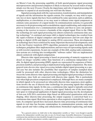
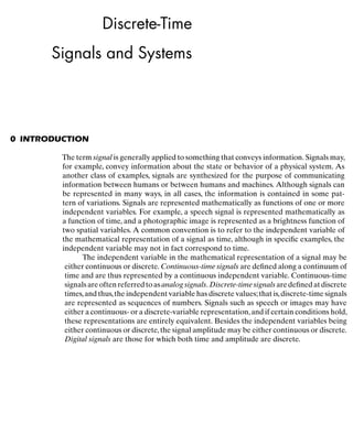
![Discrete-Time Signals and Systems
Signal-processing systems may be classified along the same lines as signals. That
is, continuous-time systems are systems for which both the input and the output are
continuous-time signals, and discrete-time systems are those for which both the input
and the output are discrete-time signals. Similarly, a digital system is a system for which
both the input and the output are digital signals. Digital signal processing, then, deals
with the transformation of signals that are discrete in both amplitude and time. The
principalfocusofthisbookisondiscrete-time—ratherthandigital—signalsandsystems.
However, the theory of discrete-time signals and systems is also exceedingly useful for
digital signals and systems, particularly if the signal amplitudes are finely quantized.
In this chapter, we present the basic definitions, establish notation, and develop
and review the basic concepts associated with discrete-time signals and systems. The
presentation of this material assumes that the reader has had previous exposure to some
of this material, perhaps with a different emphasis and notation. Thus, this chapter is
primarily intended to provide a common foundation for more advanced material.
In Section 1, we discuss the representation of discrete-time signals as sequences
and describe the basic sequences such as the unit impulse, the unit step, and com-
plex exponential, which play a central role in characterizing discrete-time systems and
form building blocks for more general sequences. In Section 2,the representation,basic
properties, and simple examples of discrete-time systems are presented. Sections 3 and
4 focus on the important class of linear time-invariant (LTI) systems and their time-
domain representation through the convolution sum, with Section 5 considering the
specific class of LTI systems represented by linear,constant–coefficient difference equa-
tions. Section 6 develops the frequency domain representation of discrete-time systems
through the concept of complex exponentials as eigenfunctions, and Sections 7, 8, and 9
develop and explore the Fourier transform representation of discrete-time signals as a
linear combination of complex exponentials. Section 10 provides a brief introduction
to discrete-time random signals.
1 DISCRETE-TIME SIGNALS
Discrete-time signals are represented mathematically as sequences of numbers.
A sequence of numbers x, in which the nth number in the sequence is denoted x[n],1 is
formally written as
x = {x[n]}, −∞ < n < ∞, (1)
where n is an integer. In a practical setting,such sequences can often arise from periodic
sampling of an analog (i.e.,continuous-time) signal xa(t). In that case,the numeric value
of the nth number in the sequence is equal to the value of the analog signal, xa(t), at
time nT: i.e.,
x[n] = xa(nT ), −∞ < n < ∞. (2)
The quantity T is the sampling period, and its reciprocal is the sampling frequency.
Although sequences do not always arise from sampling analog waveforms, it is con-
venient to refer to x[n] as the “nth sample” of the sequence. Also, although, strictly
1Note that we use [ ] to enclose the independent variable of discrete-variable functions, and we use ( )
to enclose the independent variable of continuous-variable functions.
12](https://image.slidesharecdn.com/7667-250627124216-9b5d3572/85/Discrete-Time-Signal-Processing-3rd-Edition-Alan-V-Oppenheim-18-320.jpg)
![Discrete-Time Signals and Systems
speaking, x[n] denotes the nth number in the sequence, the notation of Eq. (1) is of-
ten unnecessarily cumbersome, and it is convenient and unambiguous to refer to “the
sequence x[n]” when we mean the entire sequence, just as we referred to “the analog
signal xa(t).” We depict discrete-time signals (i.e., sequences) graphically, as shown in
Figure 1.Although the abscissa is drawn as a continuous line,it is important to recognize
that x[n] is defined only for integer values of n. It is not correct to think of x[n] as being
zero when n is not an integer; x[n] is simply undefined for noninteger values of n.
–9 –7 –5 –3
–4
–6
–8 0 1 2 3 4 5 6
7 8 9 10 11
–1
–2
x[0]
x[1]
x[2]
x[n]
x[–1]
x[–2]
n Figure 1 Graphic representation of a
discrete-time signal.
As an example of a sequence obtained by sampling, Figure 2(a) shows a segment
of a speech signal corresponding to acoustic pressure variation as a function of time,and
Figure 2(b) presents a sequence of samples of the speech signal. Although the original
speech signal is defined at all values of time t, the sequence contains information about
the signal only at discrete instants. The sampling theorem guarantees that the original
32 ms
(a)
256 samples
(b)
Figure 2 (a) Segment of a continuous-time speech signal xa(t ). (b) Sequence of samples
x[n] = xa(nT ) obtained from the signal in part (a) with T = 125 μs.
13](https://image.slidesharecdn.com/7667-250627124216-9b5d3572/85/Discrete-Time-Signal-Processing-3rd-Edition-Alan-V-Oppenheim-19-320.jpg)
![Discrete-Time Signals and Systems
signal can be reconstructed as accurately as desired from a corresponding sequence of
samples if the samples are taken frequently enough.
In discussing the theory of discrete-time signals and systems, several basic se-
quences are of particular importance. These sequences are shown in Figure 3 and will
be discussed next.
The unit sample sequence (Figure 3a) is defined as the sequence
δ[n] =
0, n = 0,
1, n = 0.
(3)
The unit sample sequence plays the same role for discrete-time signals and systems that
the unit impulse function (Dirac delta function) does for continuous-time signals and
systems. For convenience, we often refer to the unit sample sequence as a discrete-time
impulse or simply as an impulse. It is important to note that a discrete-time impulse
does not suffer from the mathematic complications of the continuous-time impulse; its
definition in Eq. (3) is simple and precise.
1
Unit sample
0
(a)
n
1
Unit step
0
(b)
...
...
...
...
n
Real exponential
0
(c)
n
Sinusoidal
0
(d)
...
...
...
...
n
Figure 3 Some basic sequences. The
sequences shown play important roles
in the analysis and representation of
discrete-time signals and systems.
14](https://image.slidesharecdn.com/7667-250627124216-9b5d3572/85/Discrete-Time-Signal-Processing-3rd-Edition-Alan-V-Oppenheim-20-320.jpg)
![Discrete-Time Signals and Systems
1
0 3 4 5 6 8
7
2
–2
–4
p[n]
n
a–3
a1
a2
a7
Figure 4 Example of a sequence to be
represented as a sum of scaled, delayed
impulses.
One of the important aspects of the impulse sequence is that an arbitrary sequence
can be represented as a sum of scaled,delayed impulses. For example,the sequence p[n]
in Figure 4 can be expressed as
p[n] = a−3δ[n + 3] + a1δ[n − 1] + a2δ[n − 2] + a7δ[n − 7]. (4)
More generally, any sequence can be expressed as
x[n] =
∞
k=−∞
x[k]δ[n − k]. (5)
We will make specific use of Eq. (5) in discussing the representation of discrete-time
linear systems.
The unit step sequence (Figure 3b) is defined as
u[n] =
1, n ≥ 0,
0, n 0.
(6)
The unit step is related to the unit impulse by
u[n] =
n
k=−∞
δ[k]; (7)
that is, the value of the unit step sequence at (time) index n is equal to the accumulated
sum of the value at index n and all previous values of the impulse sequence. An alterna-
tive representation of the unit step in terms of the impulse is obtained by interpreting
the unit step in Figure 3(b) in terms of a sum of delayed impulses, as in Eq. (5). In this
case, the nonzero values are all unity, so
u[n] = δ[n] + δ[n − 1] + δ[n − 2] + · · · (8a)
or
u[n] =
∞
k=0
δ[n − k]. (8b)
As yet another alternative, the impulse sequence can be expressed as the first backward
difference of the unit step sequence, i.e.,
δ[n] = u[n] − u[n − 1]. (9)
Exponential sequences are another important class of basic signals. The general
form of an exponential sequence is
x[n] = A αn
. (10)
If A and α are real numbers, then the sequence is real. If 0 α 1 and A is positive,
then the sequence values are positive and decrease with increasing n, as in Figure 3(c).
15](https://image.slidesharecdn.com/7667-250627124216-9b5d3572/85/Discrete-Time-Signal-Processing-3rd-Edition-Alan-V-Oppenheim-21-320.jpg)
![Discrete-Time Signals and Systems
For −1 α 0, the sequence values alternate in sign but again decrease in magnitude
with increasing n. If |α| 1, then the sequence grows in magnitude as n increases.
The exponential sequence A αn with α complex has real and imaginary parts that
are exponentially weighted sinusoids. Specifically, if α = |α|ejω0 and A = |A |ejφ, the
sequence A αn can be expressed in any of the following ways:
x[n] = A αn
= |A |ejφ
|α|n
ejω0n
= |A | |α|n
ej(ω0n+φ)
(11)
= |A | |α|n
cos(ω0n + φ) + j|A | |α|n
sin(ω0n + φ).
The sequence oscillates with an exponentially growing envelope if |α| 1 or with an
exponentially decaying envelope if |α| 1. (As a simple example, consider the case
ω0 = π.)
When |α| = 1, the sequence has the form
x[n] = |A |ej(ω0n+φ)
= |A | cos(ω0n + φ) + j|A | sin(ω0n + φ); (12)
that is,the real and imaginary parts of ejω0n vary sinusoidally with n. By analogy with the
continuous-time case, the quantity ω0 is called the frequency of the complex sinusoid
or complex exponential, and φ is called the phase. However, since n is a dimensionless
integer, the dimension of ω0 is radians. If we wish to maintain a closer analogy with the
continuous-time case, we can specify the units of ω0 to be radians per sample and the
units of n to be samples.
The fact that n is always an integer in Eq. (12) leads to some important differences
between the properties of discrete-time and continuous-time complex exponential se-
quences and sinusoidal sequences. Consider, for example, a frequency (ω0 +2π). In this
case,
x[n] = A ej(ω0+2π)n
= A ejω0nej2πn = A ejω0n.
(13)
Generally, complex exponential sequences with frequencies (ω0 + 2πr), where r is an
integer, are indistinguishable from one another. An identical statement holds for sinu-
soidal sequences. Specifically, it is easily verified that
x[n] = A cos[(ω0 + 2πr)n + φ]
= A cos(ω0n + φ).
(14)
When discussing complex exponential signals of the form x[n] = A ejω0n or real sinu-
soidal signals of the form x[n] = A cos(ω0n + φ), we need only consider frequencies in
an interval of length 2π. Typically, we will choose either −π ω0 ≤ π or 0 ≤ ω0 2π.
Another important difference between continuous-time and discrete-time com-
plex exponentials and sinusoids concerns their periodicity in n. In the continuous-time
case,a sinusoidal signal and a complex exponential signal are both periodic in time with
the period equal to 2π divided by the frequency. In the discrete-time case, a periodic
sequence is a sequence for which
x[n] = x[n + N ], for all n, (15)
16](https://image.slidesharecdn.com/7667-250627124216-9b5d3572/85/Discrete-Time-Signal-Processing-3rd-Edition-Alan-V-Oppenheim-22-320.jpg)
![Discrete-Time Signals and Systems
where the period N is necessarily an integer. If this condition for periodicity is tested
for the discrete-time sinusoid, then
A cos(ω0n + φ) = A cos(ω0n + ω0N + φ), (16)
which requires that
ω0N = 2πk, (17)
where k is an integer. A similar statement holds for the complex exponential sequence
Cejω0n; that is, periodicity with period N requires that
ejω0(n+N)
= ejω0n
, (18)
which is true only for ω0N = 2πk, as in Eq. (17). Consequently, complex exponential
and sinusoidal sequences are not necessarily periodic in n with period (2π/ω0) and,
depending on the value of ω0, may not be periodic at all.
Example 1 Periodic and Aperiodic Discrete-Time Sinusoids
Consider the signal x1[n] = cos(πn/4). This signal has a period of N = 8. To show this,
note that x[n + 8] = cos(π(n + 8)/4) = cos(πn/4 + 2π) = cos(πn/4) = x[n], satisfying
the definition of a discrete-time periodic signal. Contrary to continuous-time sinusoids,
increasing the value of ω0 for a discrete-time sinusoid does not necessarily decrease
the period of the signal. Consider the discrete-time sinusoid x2[n] = cos(3πn/8),which
has a higher frequency than x1[n]. However, x2[n] is not periodic with period 8, since
x2[n + 8] = cos(3π(n + 8)/8) = cos(3πn/8 + 3π) = −x2[n]. Using an argument anal-
ogous to the one for x1[n], we can show that x2[n] has a period of N = 16. Thus,
increasing the value of ω0 = 2π/8 to ω0 = 3π/8 also increases the period of the signal.
This occurs because discrete-time signals are defined only for integer indices n.
The integer restriction on n results in some sinusoidal signals not being periodic
at all. For example, there is no integer N such that the signal x3[n] = cos(n) satisfies
the condition x3[n + N ] = x3[n] for all n. These and other properties of discrete-time
sinusoids that run counter to their continuous-time counterparts are caused by the
limitation of the time index n to integers for discrete-time signals and systems.
When we combine the condition of Eq. (17) with our previous observation that
ω0 and (ω0 + 2πr) are indistinguishable frequencies, it becomes clear that there are N
distinguishable frequencies for which the corresponding sequences are periodic with
period N. One set of frequencies is ωk = 2πk/N, k = 0, 1, . . . , N − 1. These properties
of complex exponential and sinusoidal sequences are basic to both the theory and the
design of computational algorithms for discrete-time Fourier analysis.
Related to the preceding discussion is the fact that the interpretation of high
and low frequencies is somewhat different for continuous-time and discrete-time sinu-
soidal and complex exponential signals. For a continuous-time sinusoidal signal x(t) =
A cos(0t + φ), as 0 increases, x(t) oscillates progressively more rapidly. For the
discrete-time sinusoidal signal x[n] = A cos(ω0n + φ), as ω0 increases from ω0 = 0 to-
ward ω0 = π, x[n] oscillates progressively more rapidly. However, as ω0 increases from
ω0 = π to ω0 = 2π, the oscillations become slower. This is illustrated in Figure 5. In
17](https://image.slidesharecdn.com/7667-250627124216-9b5d3572/85/Discrete-Time-Signal-Processing-3rd-Edition-Alan-V-Oppenheim-23-320.jpg)
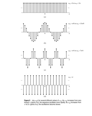
![Discrete-Time Signals and Systems
fact, because of the periodicity in ω0 of sinusoidal and complex exponential sequences,
ω0 = 2π is indistinguishable from ω0 = 0, and, more generally, frequencies around
ω0 = 2π are indistinguishable from frequencies around ω0 = 0. As a consequence, for
sinusoidal and complex exponential signals, values of ω0 in the vicinity of ω0 = 2πk
for any integer value of k are typically referred to as low frequencies (relatively slow
oscillations),whereas values of ω0 in the vicinity of ω0 = (π+2πk) for any integer value
of k are typically referred to as high frequencies (relatively rapid oscillations).
2 DISCRETE-TIME SYSTEMS
A discrete-time system is defined mathematically as a transformation or operator that
maps an input sequence with values x[n] into an output sequence with values y[n]. This
can be denoted as
y[n] = T{x[n]} (19)
and is indicated pictorially in Figure 6. Equation (19) represents a rule or formula for
computing the output sequence values from the input sequence values. It should be
emphasized that the value of the output sequence at each value of the index n may
depend on input samples x[n] for all values of n, i.e., y at time n can depend on all or
part of the entire sequence x. The following examples illustrate some simple and useful
systems.
x[n] y[n]
T{•}
Figure 6 Representation of a
discrete-time system, i.e., a
transformation that maps an input
sequence x[n] into a unique output
sequence y[n].
Example 2 The Ideal Delay System
The ideal delay system is defined by the equation
y[n] = x[n − nd], −∞ n ∞, (20)
where nd is a fixed positive integer representing the delay of the system. In other words,
the ideal delay system shifts the input sequence to the right by nd samples to form the
output. If, in Eq. (20), nd is a fixed negative integer, then the system would shift the
input to the left by |nd| samples, corresponding to a time advance.
In the system of Example 2, only one sample of the input sequence is involved in
determining a certain output sample. In the following example, this is not the case.
19](https://image.slidesharecdn.com/7667-250627124216-9b5d3572/85/Discrete-Time-Signal-Processing-3rd-Edition-Alan-V-Oppenheim-25-320.jpg)
![Discrete-Time Signals and Systems
Example 3 Moving Average
The general moving-average system is defined by the equation
y[n] =
1
M1 + M2 + 1
M2
k=−M1
x[n − k]
=
1
M1 + M2 + 1
{x[n + M1] + x[n + M 1 − 1] + · · · + x[n] (21)
+x[n − 1] + · · · + x[n − M2]} .
This system computes the nth sample of the output sequence as the average of (M1 +
M2 +1) samples of the input sequence around the nth sample. Figure 7 shows an input
sequenceplottedasafunctionofadummyindexk andthesamples(soliddots)involved
in the computation of the output sample y[n] for n = 7, M 1 = 0, and M2 = 5. The out-
put sample y[7] is equal to one-sixth of the sum of all the samples between the vertical
dotted lines. To compute y[8], both dotted lines would move one sample to the right.
x[k]
k
n
0
n – 5
Figure 7 Sequence values involved in computing a moving average with M1 = 0
and M2 = 5.
Classes of systems are defined by placing constraints on the properties of the
transformation T {·}. Doing so often leads to very general mathematical representa-
tions, as we will see. Of particular importance are the system constraints and properties,
discussed in Sections 2.1–2.5.
2.1 Memoryless Systems
A system is referred to as memoryless if the output y[n] at every value of n depends
only on the input x[n] at the same value of n.
Example 4 A Memoryless System
An example of a memoryless system is a system for which x[n] and y[n] are related by
y[n] = (x[n])2, for each value of n. (22)
20](https://image.slidesharecdn.com/7667-250627124216-9b5d3572/85/Discrete-Time-Signal-Processing-3rd-Edition-Alan-V-Oppenheim-26-320.jpg)
![Discrete-Time Signals and Systems
The system in Example 2 is not memoryless unless nd = 0; in particular, that
system is referred to as having “memory” whether nd is positive (a time delay) or
negative (a time advance). The moving average system in Example 3 is not memoryless
unless M1 = M2 = 0.
2.2 Linear Systems
The class of linear systems is defined by the principle of superposition. If y1[n] and y2[n]
are the responses of a system when x1[n] and x2[n] are the respective inputs, then the
system is linear if and only if
T{x1[n] + x2[n]} = T{x1[n]} + T{x2[n]} = y1[n] + y2[n] (23a)
and
T{ax[n]} = aT{x[n]} = ay[n], (23b)
where a is an arbitrary constant. The first property is the additivity property, and the
second the homogeneity or scaling property. These two properties together comprise
the principle of superposition, stated as
T{ax1[n] + bx2[n]} = aT{x1[n]} + bT{x2[n]} (24)
for arbitrary constants a and b. This equation can be generalized to the superposition
of many inputs. Specifically, if
x[n] =
k
akxk[n], (25a)
then the output of a linear system will be
y[n] =
k
akyk[n], (25b)
where yk[n] is the system response to the input xk[n].
By using the definition of the principle of superposition, it is easily shown that the
systems of Examples 2 and 3 are linear systems. (See Problem 39.) An example of a
nonlinear system is the system in Example 4.
Example 5 The Accumulator System
The system defined by the input–output equation
y[n] =
n
k=−∞
x[k] (26)
is called the accumulator system, since the output at time n is the accumulation or
sum of the present and all previous input samples. The accumulator system is a linear
system. Since this may not be intuitively obvious, it is a useful exercise to go through
the steps of more formally showing this. We begin by defining two arbitrary inputs
x1[n] and x2[n] and their corresponding outputs
21](https://image.slidesharecdn.com/7667-250627124216-9b5d3572/85/Discrete-Time-Signal-Processing-3rd-Edition-Alan-V-Oppenheim-27-320.jpg)
![Discrete-Time Signals and Systems
y1[n] =
n
k=−∞
x1[k], (27)
y 2[n] =
n
k=−∞
x2[k]. (28)
When the input is x3[n] = ax1[n] + bx2[n], the superposition principle requires the
output y3[n] = ay1[n] + by2[n] for all possible choices of a and b. We can show this by
starting from Eq. (26):
y3[n] =
n
k=−∞
x3[k], (29)
=
n
k=−∞
(ax1[k] + bx2[k]), (30)
= a
n
k=−∞
x1[k] + b
n
k=−∞
x2[k], (31)
= ay1[n] + by2[n]. (32)
Thus, the accumulator system of Eq. (26) satisfies the superposition principle for all
inputs and is therefore linear.
Example 6 A Nonlinear System
Consider the system defined by
w[n] = log10 (|x[n]|). (33)
This system is not linear. To prove this, we only need to find one counterexample—
that is, one set of inputs and outputs which demonstrates that the system violates
the superposition principle, Eq. (24). The inputs x1[n] = 1 and x2[n] = 10 are a
counterexample. However, the output for x1[n] + x2[n] = 11 is
log10(1 + 10) = log10(11) = log10(1) + log10(10) = 1.
Also,the output for the first signal is w1[n] = 0,whereas for the second,w2[n] = 1.The
scaling property of linear systems requires that, since x2[n] = 10x1[n], if the system is
linear, it must be true that w2[n] = 10w1[n]. Since this is not so for Eq. (33) for this
set of inputs and outputs, the system is not linear.
2.3 Time-Invariant Systems
A time-invariant system (often referred to equivalently as a shift-invariant system) is
a system for which a time shift or delay of the input sequence causes a corresponding
shift in the output sequence. Specifically, suppose that a system transforms the input
sequence with values x[n] into the output sequence with values y[n]. Then, the system
is said to be time invariant if, for all n0, the input sequence with values x1[n] = x[n−n0]
produces the output sequence with values y1[n] = y[n − n0].
As in the case of linearity,proving that a system is time invariant requires a general
proofmakingnospecificassumptionsabouttheinputsignals.Ontheotherhand,proving
non-time invariance only requires a counter example to time invariance. All of the
systems in Examples 2–6 are time invariant. The style of proof for time invariance is
illustrated in Examples 7 and 8.
22](https://image.slidesharecdn.com/7667-250627124216-9b5d3572/85/Discrete-Time-Signal-Processing-3rd-Edition-Alan-V-Oppenheim-28-320.jpg)
![Discrete-Time Signals and Systems
Example 7 The Accumulator as a Time-Invariant System
Consider the accumulator from Example 5. We define x1[n] = x[n−n0]. To show time
invariance, we solve for both y[n − n0] and y1[n] and compare them to see whether
they are equal. First,
y[n − n0] =
n−n0
k=−∞
x[k]. (34)
Next, we find
y1[n] =
n
k=−∞
x1[k] (35)
=
n
k=−∞
x[k − n0]. (36)
Substituting the change of variables k1 = k − n0 into the summation gives
y1[n] =
n−n0
k1=−∞
x[k1]. (37)
Since the index k in Eq. (34) and the index k1 in Eq. (37) are dummy indices of
summation,and can have any label,Eqs. (34) and (37) are equal and therefore y1[n] =
y[n − n0]. The accumulator is a time-invariant system.
The following example illustrates a system that is not time invariant.
Example 8 The Compressor System
The system defined by the relation
y[n] = x[Mn], −∞ n ∞, (38)
with M a positive integer, is called a compressor. Specifically, it discards (M − 1)
samples out of M; i.e., it creates the output sequence by selecting every Mth sample.
This system is not time invariant.We can show that it is not by considering the response
y1[n] to the input x1[n] = x[n − n0]. For the system to be time invariant, the output of
the system when the input is x1[n] must be equal to y[n − n0]. The output y1[n] that
results from the input x1[n] can be directly computed from Eq. (38) to be
y1[n] = x1[Mn] = x[Mn − n0]. (39)
Delaying the output y[n] by n0 samples yields
y[n − n0] = x[M(n − n0)]. (40)
Comparing these two outputs, we see that y[n − n0] is not equal to y1[n] for all M and
n0, and therefore, the system is not time invariant.
It is also possible to prove that a system is not time invariant by finding a single
counterexample that violates the time-invariance property. For instance, a counterex-
ample for the compressor is the case when M = 2, x[n] = δ[n], and x1[n] = δ[n − 1].
For this choice of inputs and M, y[n] = δ[n], but y1[n] = 0; thus, it is clear that
y1[n] = y[n − 1] for this system.
23](https://image.slidesharecdn.com/7667-250627124216-9b5d3572/85/Discrete-Time-Signal-Processing-3rd-Edition-Alan-V-Oppenheim-29-320.jpg)