Heart Disease

1. Vol.:(0123456789)
SN Computer Science (2023) 4:673
https://doi.org/10.1007/s42979-023-02081-9
SN Computer Science
ORIGINAL RESEARCH
Diagnosis of Cardiac Disease Utilizing Machine Learning Techniques
and Dense Neural Networks
K. Prabhavathi1,2
· V. Mareeswari3
Received: 7 June 2023 / Accepted: 24 June 2023
© The Author(s), under exclusive licence to Springer Nature Singapore Pte Ltd 2023
Abstract
In numerous different polls, heart illnesses constantly rank among the leading causes of death. The reason behind is the
complexity of these diseases and the high prevalence of incorrect diagnoses. This is a huge obstacle for those who work in
the medical field. Since machine learning (ML) has been shown to be incredibly excellent at estimate and decision-making,
it is necessary to develop a system that can identify cardiac disease. A heart disease diagnosed in its initial phases not only
makes it possible for patients to avoid having one, but it also makes it possible for medical professionals to gain knowledge
about the primary risk factors for heart attacks and take precautions against them before they happen to a patient. In this study,
we experimented on three different datasets with different ML algorithms to diagnose heart disease. These datasets have
various medical and customary information about the patients, which are necessary elements to determine whether a patient
has heart disease or not. Hybrid model proposed by combining custom convolution neural network and extreme gradient
boosting shows better accuracy in finding heart diseases among all standard machine-learning methods. We also proposed
a custom sequential model formed with seven dense layers to diagnose a patient with cardiac disease. This proposed model
performed well, with an accuracy of 92.3% when applied to the modified Cleveland dataset.
Keywords Machine learning · Coronary heart disease (CHD) · Myocardial infarction (MI) · DT · KNN · SVM
Introduction
Heart disease is the most common, most lethal and complex
of all life-threatening conditions and can affect anyone and
primarily shows up after age 40. Several factors contribute
to heart disease, and age is only one of them, making the
possibility of heart disease seem almost arbitrary. This calls
for models that can detect abnormalities in physiological
factors that can indicate dysfunction in the behavior of the
human heart [1].
Currently, with more and more people making lifestyle
choices that are not well suited to them for the sake of their
professions or otherwise, heart disease has become more
prevalent than before [2, 3]. Heart diseases can comprise
a range of afflictions that affect the heart and can also be
called cardiovascular diseases or CVD. As per the recent
statistics of the World Health Organization, heart diseases
are prominent reason of demise worldwide. Many factors
can indicate the possibility of heart disease, and they have
been concisely depicted in Fig. 1.
Strokes are commonly caused by bleeding blood ves-
sels (hemorrhagic stroke) or the blockage of a blood vessel
with a blood clot (ischemic stroke). Most strokes are caused
by high blood pressure. Strokes are closely linked to heart
attacks, and they have similar risk factors [4].
A family history of cardiovascular diseases can also
increase an individual’s risk of developing heart diseases.
There does not exist an individual gene that causes heart
disease, but several genes coming together might be a cause
for concern [5].
This article is part of the topical collection “Advances in
Computational Approaches for Image Processing, Wireless
Networks, Cloud Applications and Network Security” guest edited
by P. Raviraj, Maode Ma and Roopashree H R.
* K. Prabhavathi
prabhavathi5218@gmail.com
V. Mareeswari
mareesh.prasanna@gmail.com
1
Department of CSE, ACSCE, Bengaluru, India
2
Department of CSE, RVITM, Bengaluru, India
3
Department of CSE, AMC Engineering College, Bengaluru,
India

2. SN Computer Science (2023) 4:673
673 Page 2 of 14
SN Computer Science
Excessive consumption of liquor is unquestionably
harmful and can lead to severe heart disorders; however,
consuming alcohol moderately has been associated with
a lowered probability of cardiovascular events occurring.
However, high alcohol consumption is proven to be injuri-
ous, and therefore, alcohol should be consumed in mod-
eration [6, 7].
Moderate to vigorous physical activity has been associ-
ated with increased cardiovascular health [8], whereas sed-
entary behavior is emerging as a factor that has a negative
impact on the cardiovascular system. Any awake habit that
involves spending fewer than 1.5 metabolic units sitting,
lying down, or otherwise reclined is considered sedentary
[9]. A study reported robust evidence that daily sitting time
was proportional and increased the risk of CVD mortality. In
order to lower the risk of getting a cardiac disease, physical
health is also crucial.
There are several complicated investigative ways to fore-
tell heart disease, which has a diverse nature and is a sig-
nificant reason that affects human life today. As a result,
heart disease therapy is particularly complicated, especially
in underdeveloped countries, due to the limited availability
of a working framework and a scarcity of doctors and other
resources that influence the expectations and treatment.
Therefore, a vast amount of information that medical ser-
vices businesses possess, some of which are veiled, is help-
ful in deciding on robust options to provide accurate results
to make practical judgments based on information. This is
where the machine-learning methods come in the picture.
Machine learning ultimately proves to be convincing in aid-
ing decision-making and anticipation from the abundance
of data provided by the medical services sector to decide on
contrary-based heart disease diagnosis.
In this study, we implemented various machine-learning
techniques on three different datasets based on historical
data collected from patients to foretell relating to a patient’s
heart condition. We also proposed a custom model based
on a sequential system made of dense layers, which yields
notable accuracy, making it an efficient model for heart dis-
ease prediction.
Related Works
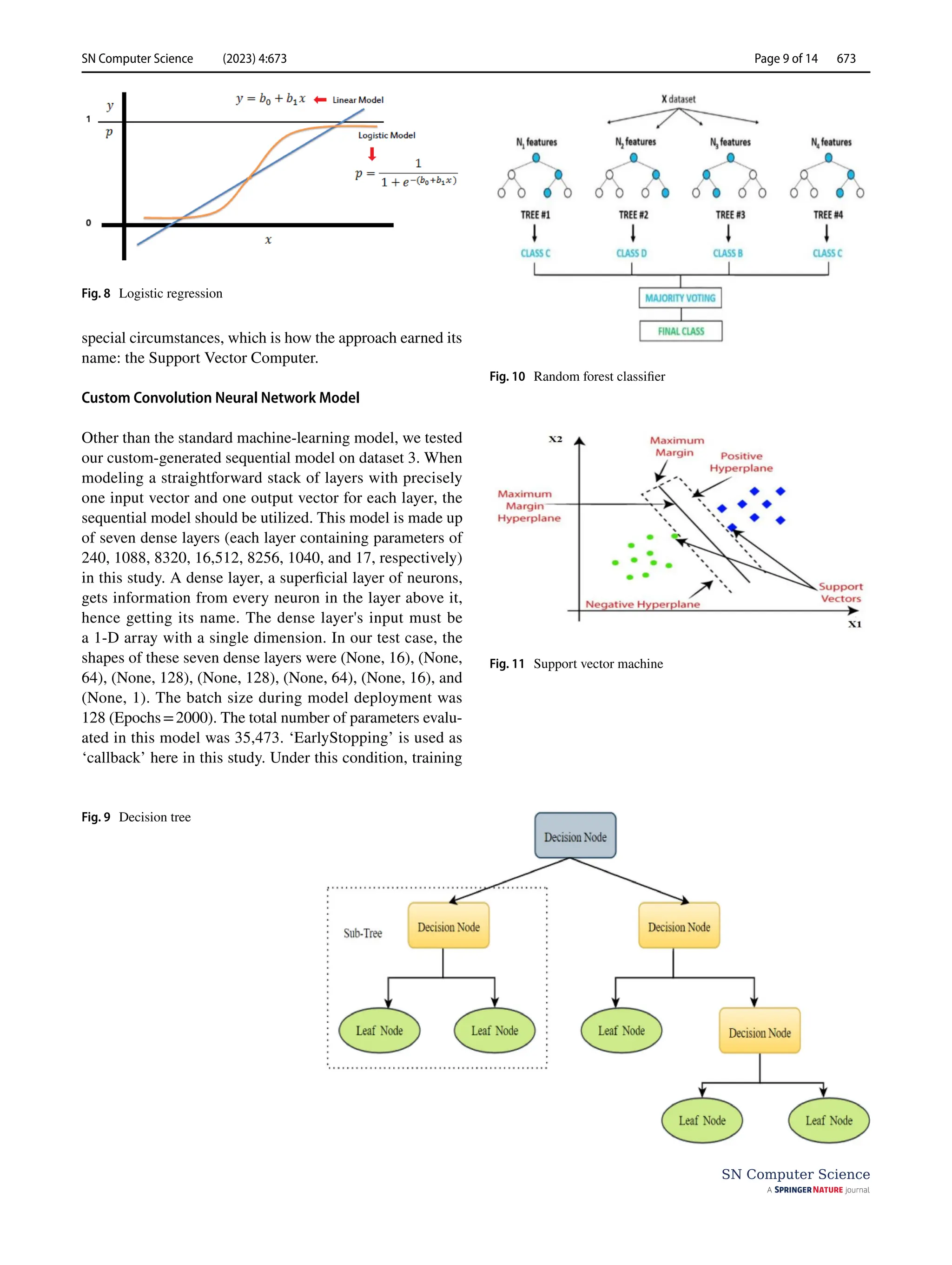
For categorizing and predicting cardiac illness, a number
of machine-learning models have been used in numerous
studies. Peter et al. suggested a technique for assessing the
results of several classification methods, including DT, NB,
KNN, NNon a dataset pertaining to heart disease [10]. They
categorize patient data and forecast who may develop cardio-
vascular problems. Melillo et al. [11] used a machine-learn-
ing method called CART, which stands for classification
and regression, to design an autonomous classifier that can
identify between patients who are at high risk of developing
congestive heart failure and patients who are at low risk.
This classifier has a sensitivity of 93.3% and a specificity of
63.5%. To enhance performance, Al Rahhal et al. [12] sug-
gested a method for analyzing electrocardiograms (ECGs)
that used deep neural networks to find the best qualities and
then apply them. Later, Dun et al. [13] experimented with
different algorithm approaches to identify heart illnesses
and hyperparameter tinkering to increase the accuracy of
the results. Using Cleveland dataset and the random forest
Fig. 1 Indicators of cardiovas-
cular disease

3. SN Computer Science (2023) 4:673 Page 3 of 14 673
SN Computer Science
method, Javeed et al. conducted research on cardiovascular
disease [14]. For the study, the author employed the Chi-
Square feature selection model in addition to the genetic
algorithm (GA)-based feature selection model. They dem-
onstrated in their experiments that their suggested model,
which uses genetic algorithms to pick features, is more accu-
rate than the models already in use. However, these find-
ings are compared to previously developed machine-learn-
ing models for evaluation. Uma et al. developed particular
criteria for identifying heart illness depending on this PSO
algorithm and then assessed various rules to arrive at a more
accurate practice [15]. Following an analysis of the criteria,
the C 5.0 system was chosen as the basis for categorizing
diseases using a binary system. In the implementation, the
author made use of data from the UCI repository, and they
assessed the high accuracy achieved by employing PSO and
the decision tree method.
It was addressed by Desai et al. how a back propaga-
tion neural network may be used to forecast cardiac disease
[16]. During the research, the authors utilized the Cleveland
dataset and Matlab to carry out the simulation. Nevertheless,
the task may be accomplished using deep learning models,
which are exceedingly precise, and this capability can be
expanded to include applications in the real world. Enriko
et al. suggested the use of data mining techniques to make
predictions regarding heart disease [17]. They used a range
of techniques and methodologies for their study and analysis,
including the KNN algorithm, the decision tree algorithm,
classifications based on neural networks, and Bayesian clas-
sification algorithms. They conducted their own experiments
using the paper, finding that the decision tree model had a
high level of accuracy.
Employed a variety of classification algorithms to identify
severe cardiac syndromes based on risk rate by the author
was used a method known as data mining utilized an artifi-
cial neural network in conjunction with a genetic algorithm
in order to forecast illnesses affecting the human body [18,
19]. The authors of this reference worked together to com-
bine the data mining approach using association rules and
classification strategies. In this aspect, the author’s model
effectively makes accurate predictions regarding cardiac ail-
ment. An in-depth discussion provided on cardiovascular
illness as well as the many signs of a heart attack. In this
study, many distinct classification and clustering approaches,
as well as the associated algorithms and tools, were utilized
[20].
An analysis utilizing data mining has been discussed.
According to the study’s findings, the accuracy of the pre-
diction of cardiac disorders varies depending on the meth-
odology utilized and the number of characteristics taken into
consideration [21, 22]. Some of the researchers examined
the findings and analyses of the UCI Machine Learning
Heart Disease dataset using a number of machine-learning
and deep learning approaches. When data pre-processing is
added to the dataset’s 13 features, the K-Neighbors classifier
fared better in the ML technique [23]. Using smartphone
technology, More et al. [24] proposed a risk factor-based
method to predict the possibility of experiencing a heart
attack. They built an android application that is connected
with bioinformatics tools comprised of the final diagnoses of
more than 500 patients hospitalized in a cardiology hospital.
Scientists have utilized a k-means clustering technique to
integrate a repository for cardiac disorders. MAFIA (Maxi-
mal Frequent Itemset Algorithm) was used to determine the
standard relevance of the most prevalent patterns that led to
heart attacks [25, 26].
Nashif et al. [27] used a cognitive method to assess a
patient’s chance of having heart disease. In this study, five
different ML algorithms were assessed for their ability to
make accurate predictions, and the results are presented. In
order to get more accurate results in prediction, a logistic
model tree was developed. This model, which employed an
ADA boost and bagging model, was used to forecast heart
disease. The findings of their investigations have shown that
random forests may attain a high level of accuracy when
making predictions. Another study with a similar approach
was done by Angraal et al. [28]. This research used classifi-
cation and regression models, namely the decision tree, the
KNN algorithm, the SVM, and the linear regression process,
to make predictions. The findings of the experiment demon-
strated that the KNN algorithm had the best degree of preci-
sion. On the other hand, this model is adaptable enough to
be used in real-time environments or applications.
Datasets and Exploratory Data Analysis
According to the Centres for Disease Control and Prevention
(CDC), heart disease affects the majority of racial and ethnic
groups in the United States [29]. Hypertension and smok-
ing are three most important risk factors for heart disease
[30], yet about half of all Americans are affected by at least
one of these risk factors. Other critical indicators include
having diabetes, having a high body mass index (BMI),
being overweight, and either not getting enough exercise
or drinking too much alcohol [31]. In medicine, it is of the
utmost importance to identify the risk factors for cardiovas-
cular disease and take preventative measures against them.
In turn, improvements in computational technology make it
possible to apply machine-learning methods to analyze data
to identify ‘patterns’ that can be used to anticipate a patient’s
status [32, 33].
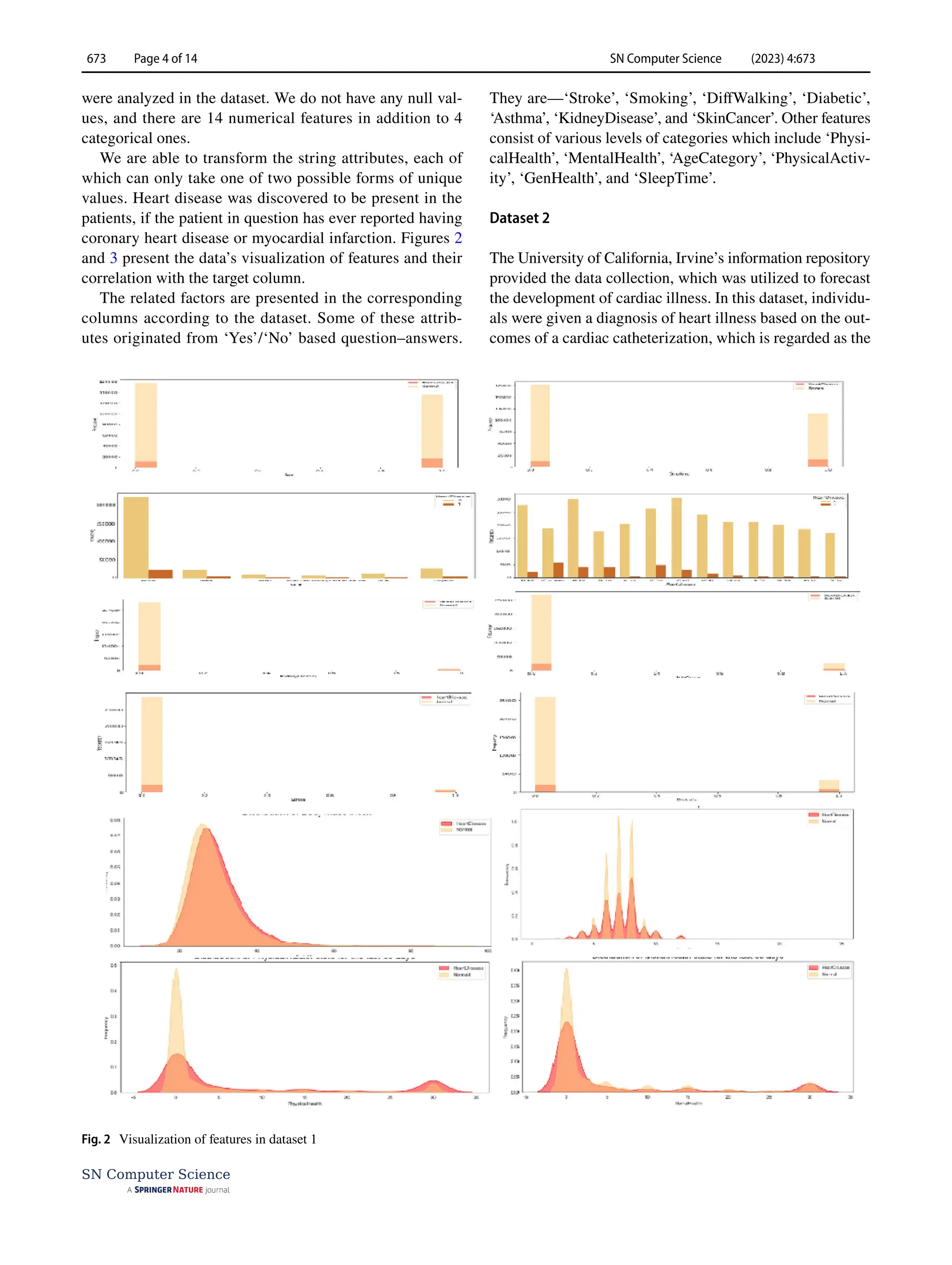
Dataset 1
This dataset was comprised of data accumulated from
319,795 numbers of patients. Here, 18 different features

4. SN Computer Science (2023) 4:673
673 Page 4 of 14
SN Computer Science
were analyzed in the dataset. We do not have any null val-
ues, and there are 14 numerical features in addition to 4
categorical ones.
We are able to transform the string attributes, each of
which can only take one of two possible forms of unique
values. Heart disease was discovered to be present in the
patients, if the patient in question has ever reported having
coronary heart disease or myocardial infarction. Figures 2
and 3 present the data’s visualization of features and their
correlation with the target column.
The related factors are presented in the corresponding
columns according to the dataset. Some of these attrib-
utes originated from ‘Yes’/‘No’ based question–answers.
They are—‘Stroke’, ‘Smoking’, ‘DiffWalking’, ‘Diabetic’,
‘Asthma’, ‘KidneyDisease’, and ‘SkinCancer’. Other features
consist of various levels of categories which include ‘Physi-
calHealth’, ‘MentalHealth’, ‘AgeCategory’, ‘PhysicalActiv-
ity’, ‘GenHealth’, and ‘SleepTime’.
Dataset 2
The University of California, Irvine’s information repository
provided the data collection, which was utilized to forecast
the development of cardiac illness. In this dataset, individu-
als were given a diagnosis of heart illness based on the out-
comes of a cardiac catheterization, which is regarded as the
Fig. 2 Visualization of features in dataset 1

5. SN Computer Science (2023) 4:673 Page 5 of 14 673
SN Computer Science
gold standard. People were considered to have a cardiac dis-
ease if one or more of their coronary arteries were narrowed
by more than fifty percent. There are a total of 270 patients
included in this cohort, and 13 various individual prognostic
factors or column features have been analyzed. The dataset
has 150 ‘absence’ cases and 120 ‘presence’ cases of heart
disease (Fig. 4).
Dataset 3
In this dataset, a patient’s presence of heart disease was
assigned from diagnosis tests. This cohort is a modified ver-
sion of dataset 2 with 303 patients. Database 3 was initially
designed to have 76 qualities, but only a portion of those
14 attributes—14 in total—are used in all of the published
research. The only database that ML researchers have spe-
cifically used up until this point is the Cleveland database.
In our test case 3, we used 14 selected attributes from this
original dataset.
The presence of cardiac disease in the patient is referred
to as the “target” area in this diagnostic technique. It is an
integer whose value might be anywhere between 0 (complete
absence) and 1. The Cleveland database has been utilized
in experiments that have prioritized presence and absence
detection over other issues. The patients’ identity details
were wiped out from the database and substituted by arti-
ficial values.
Exploratory Data Analysis
An exploratory data analysis reveals various information
about the feature columns in these datasets. The details are
described as follows:
(1) The majority of those who suffer from heart disease
are men.
(2) Heart disease affects smokers’ lives more frequently
than any other group of patients. Even if these people
do not smoke, they have heart disease conditions, sug-
gesting other contributing variables.
(3) As far as can be seen, white people have a higher risk
of developing heart disease.
(4) Heart diseases have a higher incidence rate among
those 80 years of age or older.
(5) People who reported having kidney diseases, skin can-
cer, stroke, previous exposure to diabetes, cholesterol,
etc., have a tendency to have heart disease.
(6) A greater body mass index (BMI of 35 or higher) is
significantly connected to an increased risk of cardio-
vascular disease.
(7) Both hypertension and coronary heart disease have
been associated with insomnia. A lack of quality sleep
can, over time, bring upon other bad habits that are
harmful to someone’s heart.
(8) For individuals whose physical health had been in
poor condition for 5 days or more in the past 30 days,
the majority of these individuals displayed indications
of cardiac disease.
(9) Over a period of 30 days, people who reported having
depression, anxiety, stress, or even PTSD for longer
than 3–4 days had various physiological consequences
on their bodies, including increased cardiac reactivity,
decreased blood flow to the heart, and higher cortisol
levels. This suggests that they may be at risk for devel-
oping heart conditions.
(10) Some chest pains indicate having a condition of car-
diac problems. Especially people who have reported
having angina tend to have a high risk of being diag-
nosed with CHD.
(11) The increased risk of cardiovascular diseases and
myocardial infarction was seen in patients with fast-
ing glucose levels greater than 100 mg/dL.
Fig. 3 Distribution of correlation of features in dataset 1
Fig. 4 Comparison of presence and absence of heart disease in
patients in dataset 2

6. SN Computer Science (2023) 4:673
673 Page 6 of 14
SN Computer Science
(12) An irregular EKG result may indicate the presence of
heart illness.
(13) Abnormal Max HR value may direct towards arrhyth-
mia leading to a positive sign of having cardiac dis-
ease.
Data Pre‑processing
Raw data goes through a process called data pre-processing
in order to get it ready for another procedure. Due to their
varied origin, the most real-world machine-learning datasets
are inconsistent and noisy. Applying ML techniques to noisy
data would not yield quality results because they will not
find patterns effectively. These data must be altered so that
they may be used for both training machine-learning and
artificial intelligence (AI) models and for drawing conclu-
sions from such models. During this stage, the data are con-
verted into a format that can be processed in the machine-
learning activities in a simpler and more efficient manner.
Data pre-processing is used to remove garbage and ensure
accurate test-case results. There are various stages involved
in the data pre-processing procedure. Usually, they are
depended on the dataset in use.
Data Cleaning
The data may contain a significant amount of information
that is either superfluous or absent entirely. Cleansing of
data is used to deal with this issue. The deal includes miss-
ing data, noisy data, and so on. Rectifying, fixing, or eradi-
cating inaccurate or pointless data from a dataset is called
“data cleaning.” This procedure also includes the addition
of missing data. There are instances where the data file
contains null values, which are subsequently presented as
NaN in the data-frame. ‘Fillna’ is responsible for managing
and allowing users to replace ‘NaN’ values with a value of
their own choosing. In dataset 3, we used ‘Fillna’ method to
replace some of the values of ‘Thal’ (using ‘normal’ as the
new value), ‘Ca’ (using 0.0 as the new value), etc., feature
columns.
Standardization
The bulk of machine-learning estimators developed in
scikit-learn frequently satisfy the requirement of dataset
standardization. If the various qualities do not more or
less reflect naturally dispersed data, they may behave in an
unsatisfactory manner. This is a practice of resampling the
characteristics so that their mean values are 0 and their vari-
ance values are 1. The ultimate goal of standardization is
to reduce all features to a single scale without distorting
the variances in the values’ range. It is applied on dataset 1
in the cases of the feature columns called ‘MentalHealth’,
‘BMI’, “PhysicalHealth’, and ‘SleepTime’. In the case of
dataset 2, the ‘StandardScaler’ method, which removes the
average value of the characteristics, then scales them down
to the unit variance, was used for standardization.
One‑Hot‑Encoding
The vast majority of machine-learning algorithms are unable
to operate well with categorical input and require that the
data be translated into numerical form. In addition, in some
cases, categorical columns contain more than two unique
values. We have some characteristics that each has more than
two distinct values in dataset 1. These columns are— ‘Age-
Category’, ‘Race’, and ‘GenHealth’. Similarly, in the case
of dataset 3, there are three nominal categorical variables
named—‘ChestPain’, ‘Thal’, and ‘AHD’. Hence, One-Hot-
Encoding was employed for this case in the pre-processing
step. The values that categorical (discrete) features take
on are provided as an array-like input to this transformer.
Attributes are encrypted using a one-hot or ‘dummy’ encod-
ing method. A binary column represents each category; the
result is either a dense matrix or a sparse array.
Methodology
The research could employ a variety of methodologies, such
as multiple data visualizations, data segmentation, data cre-
ation, and various machine-learning model building. This
study will primarily concentrate on the field of diagnosing
heart disease as its core area of research. According to the
conclusions of the study, the procedures described above are
the ones that should be followed in order to have the best
possibility of effectively diagnosing the presence of heart
disease from the available patient data. In this study, three
different datasets were used for experimental purposes. We
applied various machine-learning techniques to different
datasets to find the most efficient models for heart disease
detection. Figure 5 represents a simplified block diagram
of the proposed system for heart disease detection (Figs. 6
and 7).
Machine Learning Techniques Used
Machine learning (ML) is a subsection of AI that helps
software applications enhance their efficiency at predict-
ing events despite not being particularly built to execute
so. Machine learning algorithms need historic data to pro-
duce accurate output projections. They provide adequate
training on a dataset using an effective learning algorithm.
These algorithms will construct a system of regulations and
obligations, but these rules depend on the inferences drawn
from the data. When training the system, several system
models could be created using datasets from a variety of

7. SN Computer Science (2023) 4:673 Page 7 of 14 673
SN Computer Science
sources with the same learning method. The ML techniques
used in all three experiments in our study are described
below.
K‑Nearest Neighbor (KNN) KNN was developed using the
supervised learning approach. Since the fresh records and
existing cases are presumed to be comparable, this method
assigns a category to it based on how closely it resembles
the existing examples. Classifying a new data point based
on its resemblance to other data points is done by the system
in this case. It is recognized as a lazy system because instead
of using the training data instantly, it stores it and uses that
data to perform a classification action later on. During the
training phase, this algorithm does nothing more than store
the dataset; later on, when it receives new data, it catego-
rizes that data into the same subcategory as those of the cur-
rent data.
At first, the quantity K of the surrounding neighbors is
chosen. Computing the Distance measure between every
K-neighbors is the next stage. On the basis of Euclidean
distance, the physically closest K-neighbors are selected and
the sum of the data points that belong to each group of these
k-neighbors is calculated as the fourth step. The newly col-
lected data points are then assigned to the group that has the
most neighbors in that category as the process’s last step.
The KNN method was applied on all three datasets. In
K-neighbors queries, the value for the number of neighbors
was set at 5 for dataset 1.
For dataset 2, this number of ‘n_neighbors’ was set at 9.
The power parameter for the metric used here was set at 2.
The metric, in this case, is Euclidean.
Logistic Regression Nevertheless, logistic regression is
not a regression model at all, despite what its name would
imply. In comparison to other methods, when it comes
to solving binary and linear classification issues, logis-
tic regression is an efficient and effective method. When
used on classes that can be linearly separated, it is a para-
digm for categorizing data that is comparatively simple to
apply and yields great results. As a statistical tool, logistic
regression uses previously gathered data to estimate the
likelihood of the occurrence, such as electing or not elect-
ing, occurring based on a set of independent variables.
The dependent variable can take any value between 0 and
1 because the outcome is a probability. The maximal like-
lihood estimation (MLE) technique is utilized in logistic
regression in order to determine the model parameters that
correlate factors to the aim.
The equation for logistic regression can be rewritten in
terms of an odds ratio (Eq. 1):
Here, ­b0 is the constant and ­
b1 is the slope of the linear
model y:
From (1), we get
In addition, this leads to the equation of logistic regres-
sion (Eq. 4):
Logistic regression was applied to dataset 3.
(1)
p
1 − p
= e(b0+b1x)
(2)
y = b0 + b1x
(3)
ln
(
p
1 − p
)
= b0 + b1x
(4)
p =
1
1 + e(b0+b1x)
Fig. 5 Frequency of heart dis-
ease vs. sex in dataset 3

8. SN Computer Science (2023) 4:673
673 Page 8 of 14
SN Computer Science
Decision Tree Classifier
DT is a supervised approach for regression and classifica-
tion analysis issues, but predominantly classification. The
classifier in this method has the shape of a tree, with the
leaves signifying the result and the branches designating the
guidelines for making decisions. It is a graphical illustration
for discovering all feasible responses to a query or coming
to a choice based on the given parameters. The following
diagram in Fig. 8 represents a simplified version of a deci-
sion tree. The decision tree classifier model was employed
on dataset 1 (Figs. 9, 10, 11, and 13).
Random Forest Classifier
The RF approach averages how many decision trees were
applied to the various regions of the dataset that was pro-
vided. This contributes to improving the dataset’s projected
accuracy. Instead of relying just on one decision tree, the
random forest model considers each tree’s projection and
bases its conclusion on the one that obtained the most sup-
port for its prognosis. A random subset of features in a ran-
dom forest classifier is generated using feature randomness,
ensuring little correlation between decision trees. This is an
important distinction between random forests and decision
trees. Random forests take into account only a subset of the
possible features to split into, whereas decision trees take
into account all the available feature splits. Over-fitting can
be evaded by partaking a more trees to select from when
making a model in this case.
Support Vector Machine
The SVM technique looks for the optimum line or decision
boundary to partition an n-dimensional space into classes.
We will be able to classify any additional data points easily
going forward thanks to this. SVM is used to identify the
critical examples and variables that promote the formation
of the hyperplane. Support vectors are used to refer to these
Fig. 6 Block diagram of methodology
Fig. 7 KNN classifier

9. SN Computer Science (2023) 4:673 Page 9 of 14 673
SN Computer Science
special circumstances, which is how the approach earned its
name: the Support Vector Computer.
Custom Convolution Neural Network Model
Other than the standard machine-learning model, we tested
our custom-generated sequential model on dataset 3. When
modeling a straightforward stack of layers with precisely
one input vector and one output vector for each layer, the
sequential model should be utilized. This model is made up
of seven dense layers (each layer containing parameters of
240, 1088, 8320, 16,512, 8256, 1040, and 17, respectively)
in this study. A dense layer, a superficial layer of neurons,
gets information from every neuron in the layer above it,
hence getting its name. The dense layer's input must be
a 1-D array with a single dimension. In our test case, the
shapes of these seven dense layers were (None, 16), (None,
64), (None, 128), (None, 128), (None, 64), (None, 16), and
(None, 1). The batch size during model deployment was
128 (Epochs=2000). The total number of parameters evalu-
ated in this model was 35,473. ‘EarlyStopping’ is used as
‘callback’ here in this study. Under this condition, training
Fig. 8 Logistic regression
Fig. 9 Decision tree
Fig. 10 Random forest classifier
Fig. 11 Support vector machine

10. SN Computer Science (2023) 4:673
673 Page 10 of 14
SN Computer Science
gets terminated immediately whenever an observed metric
ceases progressing.
Extreme Gradient Boosting (XGBoost)‑Proposed
Model
Gradient boosting algorithm is utilized to anticipate the
target by combining evaluations of a lot of less complex
models. It maps the information highlight to its leaves which
possess a nonstop score. XGBoost limits a regularized target
work that joins a curved misfortune in particular multifac-
eted nature. The preparation continues repetitively by includ-
ing new set of trees to foresee the mistakes in earlier ones in
order to join them with the prior ones. Henceforth termed as
angle boosting on the grounds that it utilizes an inclination
plunge calculation to limit the loss. In order to minimize the
next goal, we must add ft to the formal forecast made by y
_i((t)) for the i-th instance at the t-th iteration:
This suggests that we incorporate ­
ft, which enhances our
model. In the generic setting, the aim can be quickly opti-
mized using second-order approximation:
The loss function’s first- and second-order gradient sta-
tistics are g_i = _(y_i((t−1))) l(y_i,y_i((t−1))) and h_i = _
(y_i((t−1))))2. We can remove the constant terms at step t
to accomplish the more direct objective described as follows:
The instance set of leaf j is defined as Ij ={i|q(xi)=j} By
expanding, we can reformat Eq. (1) as follows:
(5)
L(t)
=
n
∑
i=1
l(yi, ̂
y(t−1)
i
+ ft(xi)) + Ω(ft)
(6)
L(t)
≃
n
∑
i=1
[
l
(
yi, ̂
y(t−1)
i
)
+ gift(xi) +
1
2
hif2
t
(xi)
]
+ Ω (ft)
(7)
̃
L
(t)
=
n
∑
i=1
[
gift(xi) +
1
2
hif2
t
(xi)
]
+ Ω(ft)
(8)
̃
L
(t)
=
n
�
i=1
�
gift(xi) +
1
2
hif2
t
(xi)
�
+ 𝛾 T +
1
2
𝜆
T
�
j=1
w2
j
=
T
�
j=1
⎡
⎢
⎢
⎢
�
�
i∈Ij
gi
�
wj +
1
2
⎛
⎜
⎜
⎝
�
i∈Ij
hi + 𝜆
⎞
⎟
⎟
⎠
w2
j
⎤
⎥
⎥
⎥
+ 𝛾T
For a fixed structure q(x), we find the optimum weight
w_j* of leaf j by
and determine the associated value by
We combined weighted CNN and XGBoost and for pre-
dicting the heart disease presence and absence classes.
Results and Discussion
This study aims to identify the presence or absence of a
cardiac disease issue. Various classification techniques such
as DT classifier, RF classifier, LR, KNN, and SVM were
utilized to classify the heart disease condition (‘Yes’/‘No’
or ‘present’/‘absent’) in patients.
The Performance of the Models
We used various equations to determine the performance
of the models used in this study. Usually, a classification
algorithm’s performance is evaluated using a table called
a confusion matrix (Table 1). In a confusion matrix, each
row denotes a real class, whereas each column indicates a
predicted class.
From the confusion matrix, we get various parameters to
measure the performance and efficiency of a model. They
are presented in Eqs. (10–16):
(9)
w∗
j
= −
∑
i∈Ij
gi
∑
i∈Ij
hi + 𝜆
,
(10)
̃
L
(t)
= −
1
2
T
�
i=1
�∑
i∈Ij
gi
�
∑
i∈Ij
hi + 𝜆
+ 𝛾T
(11)
Total Predicted Positive = True Positive + False Positive
(12)
Total Actual Positive = True Positive + False Negative
(13)
Precision =
True Positive
Total Predicted Positive
(14)
Recall =
True Positive
Total Active Positive
(15)
F1score = 2
(
Precision × Recall
Precision + Recall
)
(16)
Accuarcy =
True Positive + TrueNegative
(True Positive + True Negative + False Positive + False Negative)

11. SN Computer Science (2023) 4:673 Page 11 of 14 673
SN Computer Science
Here p0 and pe indicate observed and expected agreement,
respectively.
(17)
Cohen’s kappa score =
p0 − pe
1 − pe
Another performance parameter is the ROC curve
which is the graph of receiver operating characteristics.
This graph is plotted using a true-positive rate and a false-
positive rate. Figure 11 presents the evaluation metrics and
ROC curve plots for the decision tree and KNN models
[34]. From the evaluation metrics (Table 2) of the deci-
sion tree and KNN model employed on dataset 1, it is seen
that custom CNN with combination of weighted XGBoost
gives better result when employed on dataset 1.
In Experiment 2, three different models were employed
on dataset 2. They were supporting vector machine, KNN,
and decision tree classifier. These models accurately pre-
dicted 95 heart disease conditions, but all of their other per-
formance parameters differed (Table 3). Both support vector
machine and KNN models were close enough in the cases of
Fig. 12 Model comparison for heart disease detection for decision tree and KNN models: evaluation metrics plot (left) and ROC curve (right)
Fig. 13 Graphical representa-
tion of accuracy, loss, validation
accuracy, and validation loss
for the custom model when
employed on dataset 3
Table 1 The confusion matrix
Actual Predicted
Negative Positive
Negative True negative False positive
Positive False negative True positive

12. SN Computer Science (2023) 4:673
673 Page 12 of 14
SN Computer Science
precision, recall, and F1-scores. The support vector machine
shows an accuracy of 77%, which is greater than the other
two classifiers.
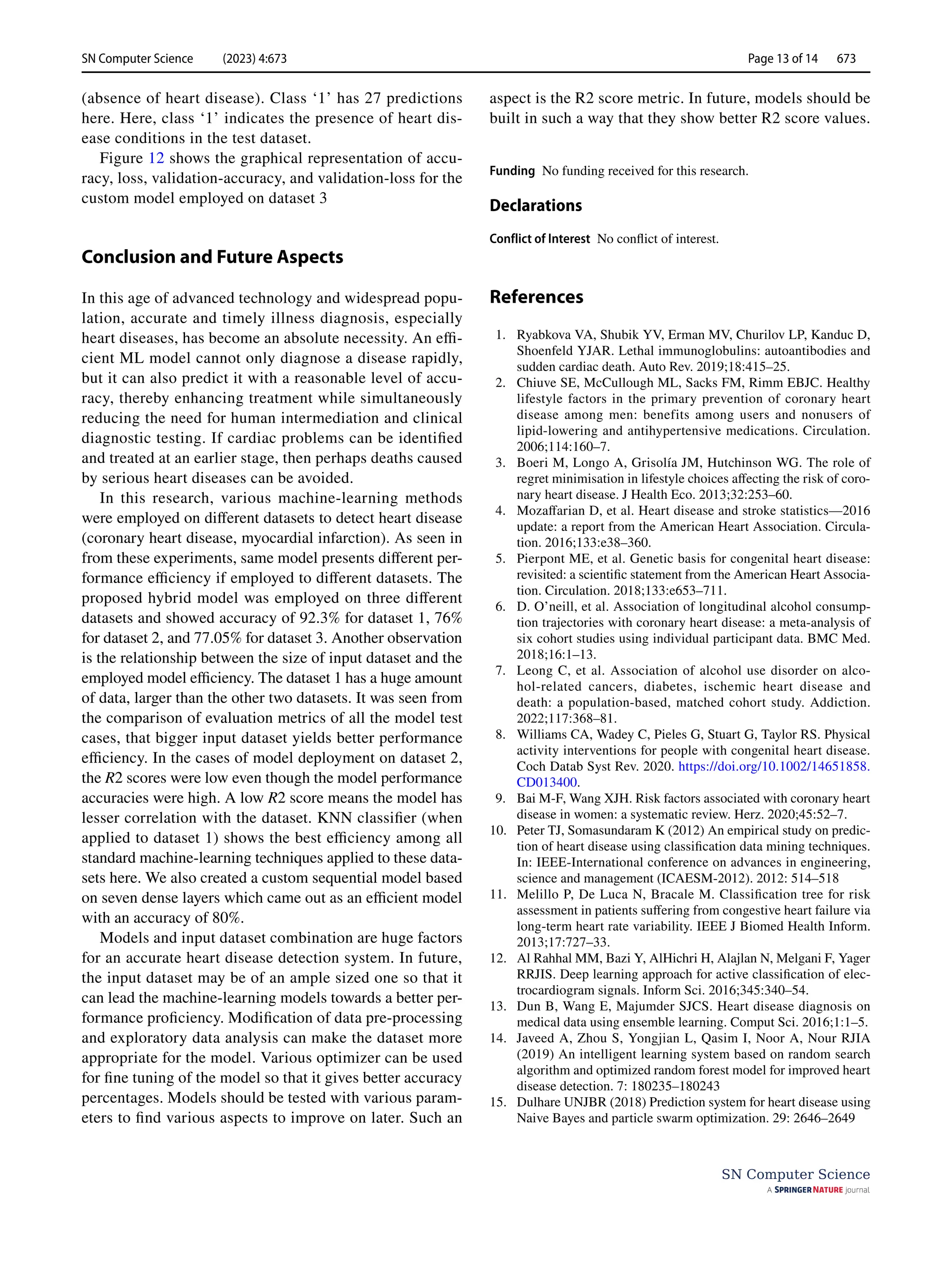
In Experiment 3, we employed four different machine-
learning classifier models on dataset 4. The first three were
logistic regression, random forest, and k-nearest neighbor
classification techniques. Two new performance parameters
which are called the R2 score and the AUC score, respec-
tively, were used in this experiment for comparison of model
performances [35, 36]. The R2 score works by figuring out
how much of the variation in predictions the dataset can
account for. Simply put, it is the difference between the pre-
dictions made by the model and the dataset’s samples. These
three models show R2 scores of 26.91%, 13.62%, and 6.97%.
The efficiency of a classifier to differentiate among classes
is measured by the Area-Under-the-Curve (AUC), which is
used as a synopsis of the ROC curve. The model is doing
better when it comes to differentiating between the positive
and unfavorable categories when the AUC value is larger.
These various performance metric values are presented in
Table 3 for the performance comparison of classifier models
used in Experiment 3.
The fourth model in Experiment 3 is a custom sequen-
tial model prepared by us. This model shows an accu-
racy of 80%, making itself an efficient classifier. The
performance metrics details of this model are presented
in Table 4. This model accurately predicts 61 instances.
Thirty-four of these predictions belonged to the ‘0’ class
Table 2 Comparison of
evaluation metrics for different
models in experiment 1
Build models Class Precision Recall F1-score Accuracy
Logistic regression 0 0.67 0.70 0.69 67.58
1 0.66 0.68 0.67
Random forest 0 0.76 0.77 0.77 75.72
1 0.75 0.76 0.76
KNN 0 0.80 0.78 0.79 76%
1 0.71 0.72 0.72
DT 0 0.73 0.65 0.69 77%
1 0.59 0.68 0.63
SVM 0 0.80 0.80 0.80 66%
1 0.72 0.72 0.73
Simple XGBoost 0 0.93 0.81 0.86 86.75
1 0.82 0.93 0.87
Weighted XGBoost 0 0.93 0.83 0.87 87.73
1 0.83 0.93 0.88
Simple CNN 0 0.86 0.83 0.84 84.58
1 0.83 0.87 0.85
Weighted CNN 0 0.86 0.88 0.87 87.24
1 0.89 0.87 0.88
Simple CNN+simple XGBoost 0 0.87 0.88 0.88 88.06
1 0.89 0.88 0.88
Simple CNN+weighted XGBoost 0 0.90 0.86 0.88 88.36
1 0.87 0.91 0.89
Custom CNN+weighted XGBoost 0 0.93 0.91 0.92 92.30
1 0.92 0.93 0.93
Table 3 Comparison of
evaluation metrics for different
models in experiment 3
Accuracy (%) Precision (%) Recall (%) F1 Score AUC score (%)
Logistic regression 81.97 80.77 77.78 0.7925 81.54
Random forest 78.69 76.92 74.07% 0.7547 78.21
KNN 77.05 76.00 70.37% 0.7308 76.36
Table 4 Evaluation metrics for custom sequential model
Model Accuracy Precision Recall (%) F1 score Support
Custom
sequential
80% 0 82 0.82 34
model 1 78 0.78 27

13. SN Computer Science (2023) 4:673 Page 13 of 14 673
SN Computer Science
(absence of heart disease). Class ‘1’ has 27 predictions
here. Here, class ‘1’ indicates the presence of heart dis-
ease conditions in the test dataset.
Figure 12 shows the graphical representation of accu-
racy, loss, validation-accuracy, and validation-loss for the
custom model employed on dataset 3
Conclusion and Future Aspects
In this age of advanced technology and widespread popu-
lation, accurate and timely illness diagnosis, especially
heart diseases, has become an absolute necessity. An effi-
cient ML model cannot only diagnose a disease rapidly,
but it can also predict it with a reasonable level of accu-
racy, thereby enhancing treatment while simultaneously
reducing the need for human intermediation and clinical
diagnostic testing. If cardiac problems can be identified
and treated at an earlier stage, then perhaps deaths caused
by serious heart diseases can be avoided.
In this research, various machine-learning methods
were employed on different datasets to detect heart disease
(coronary heart disease, myocardial infarction). As seen in
from these experiments, same model presents different per-
formance efficiency if employed to different datasets. The
proposed hybrid model was employed on three different
datasets and showed accuracy of 92.3% for dataset 1, 76%
for dataset 2, and 77.05% for dataset 3. Another observation
is the relationship between the size of input dataset and the
employed model efficiency. The dataset 1 has a huge amount
of data, larger than the other two datasets. It was seen from
the comparison of evaluation metrics of all the model test
cases, that bigger input dataset yields better performance
efficiency. In the cases of model deployment on dataset 2,
the R2 scores were low even though the model performance
accuracies were high. A low R2 score means the model has
lesser correlation with the dataset. KNN classifier (when
applied to dataset 1) shows the best efficiency among all
standard machine-learning techniques applied to these data-
sets here. We also created a custom sequential model based
on seven dense layers which came out as an efficient model
with an accuracy of 80%.
Models and input dataset combination are huge factors
for an accurate heart disease detection system. In future,
the input dataset may be of an ample sized one so that it
can lead the machine-learning models towards a better per-
formance proficiency. Modification of data pre-processing
and exploratory data analysis can make the dataset more
appropriate for the model. Various optimizer can be used
for fine tuning of the model so that it gives better accuracy
percentages. Models should be tested with various param-
eters to find various aspects to improve on later. Such an
aspect is the R2 score metric. In future, models should be
built in such a way that they show better R2 score values.
Funding No funding received for this research.
Declarations
Conflict of Interest No conflict of interest.
References
1. Ryabkova VA, Shubik YV, Erman MV, Churilov LP, Kanduc D,
Shoenfeld YJAR. Lethal immunoglobulins: autoantibodies and
sudden cardiac death. Auto Rev. 2019;18:415–25.
2. Chiuve SE, McCullough ML, Sacks FM, Rimm EBJC. Healthy
lifestyle factors in the primary prevention of coronary heart
disease among men: benefits among users and nonusers of
lipid-lowering and antihypertensive medications. Circulation.
2006;114:160–7.
3. Boeri M, Longo A, Grisolía JM, Hutchinson WG. The role of
regret minimisation in lifestyle choices affecting the risk of coro-
nary heart disease. J Health Eco. 2013;32:253–60.
4. Mozaffarian D, et al. Heart disease and stroke statistics—2016
update: a report from the American Heart Association. Circula-
tion. 2016;133:e38–360.
5. Pierpont ME, et al. Genetic basis for congenital heart disease:
revisited: a scientific statement from the American Heart Associa-
tion. Circulation. 2018;133:e653–711.
6. D. O’neill, et al. Association of longitudinal alcohol consump-
tion trajectories with coronary heart disease: a meta-analysis of
six cohort studies using individual participant data. BMC Med.
2018;16:1–13.
7. Leong C, et al. Association of alcohol use disorder on alco-
hol-related cancers, diabetes, ischemic heart disease and
death: a population-based, matched cohort study. Addiction.
2022;117:368–81.
8. Williams CA, Wadey C, Pieles G, Stuart G, Taylor RS. Physical
activity interventions for people with congenital heart disease.
Coch Datab Syst Rev. 2020. https://​doi.​org/​10.​1002/​14651​858.​
CD013​400.
9. Bai M-F, Wang XJH. Risk factors associated with coronary heart
disease in women: a systematic review. Herz. 2020;45:52–7.
10. Peter TJ, Somasundaram K (2012) An empirical study on predic-
tion of heart disease using classification data mining techniques.
In: IEEE-International conference on advances in engineering,
science and management (ICAESM-2012). 2012: 514–518
11. Melillo P, De Luca N, Bracale M. Classification tree for risk
assessment in patients suffering from congestive heart failure via
long-term heart rate variability. IEEE J Biomed Health Inform.
2013;17:727–33.
12. Al Rahhal MM, Bazi Y, AlHichri H, Alajlan N, Melgani F, Yager
RRJIS. Deep learning approach for active classification of elec-
trocardiogram signals. Inform Sci. 2016;345:340–54.
13. Dun B, Wang E, Majumder SJCS. Heart disease diagnosis on
medical data using ensemble learning. Comput Sci. 2016;1:1–5.
14. Javeed A, Zhou S, Yongjian L, Qasim I, Noor A, Nour RJIA
(2019) An intelligent learning system based on random search
algorithm and optimized random forest model for improved heart
disease detection. 7: 180235–180243
15. Dulhare UNJBR (2018) Prediction system for heart disease using
Naive Bayes and particle swarm optimization. 29: 2646–2649

14. SN Computer Science (2023) 4:673
673 Page 14 of 14
SN Computer Science
16. Desai SD, Giraddi S, Narayankar P, Pudakalakatti NR, Sulegaon
S. Back-propagation neural network versus logistic regression
in heart disease classification. In: Desai SD, editor. Advanced
computing and communication technologies: Springer Singapore.
Springer Singapore; 2019.
17. Enriko IKA, Suryanegara M, Gunawan D (2018) Heart disease
diagnosis system with k-nearest neighbors method using real
clinical medical records, In: Proceedings of the 4th International
Conference on Frontiers of Educational Technologies. 127–131
18. Shaji SP, Predictionand diagnosis of heart disease patients using
data mining technique, in 2019 international conference on com-
munication and signal processing (ICCSP) 2019 0848–0852:
IEEE.
19. Reddy GT, Reddy M, Lakshmanna K, Rajput DS, Kaluri R, Sriv-
astava GJEI (2020) Hybrid genetic algorithm and a fuzzy logic
classifier for heart disease diagnosis. 13: 185–196
20. Bashir S, Khan ZS, Khan FH, Anjum A, Bashir K (2019) “Improv-
ing heart disease prediction using feature selection approaches,”
In: 2019 16th international bhurban conference on applied sci-
ences and technology (IBCAST), p. 619–623: IEEE
21. Tougui I, Jilbab A, El Mhamdi JJH (2020) Technology, 2020
Heart disease classification using data mining tools and machine
learning techniques. 10: 1137–1144
22. Nguyen T-H, Nguyen T-N, Nguyen T-T. A deep learning frame-
work for heart disease classification in an IoTs-based system. In:
Valentina E, editor. A handbook of internet of things in biomedi-
cal and cyber physical system. Springer International Publishing;
2020.
23. Bharti R, et al. 2021 Prediction of heart disease using a com-
bination of machine learning and deep learning. Comput Intell
Neurosci. 2021;2021:1.
24. More K, Raihan M, More A, Padule S, Mondal SJJH. A12176
Smart phone based “heart attack” risk prediction; innovation
of clinical and social approach for preventive cardiac health. J
Hypert. 2018;36:321.
25. Y. Liu, 2018 Environmental health nexus: designing predictive
models for improving public health interventions. University of
Minnesota
26. Dahal KR, Gautam YJOJS. “Argumentative comparative analy-
sis of machine learning on coronary artery disease. Open J Stat.
2020;10:694–705.
27. Nashif S, Raihan MR, Islam MR. Heart disease detection by using
machine learning algorithms and a real-time cardiovascular health
monitoring system. World J Eng Technol. 2018;6:854–73.
28. Angraal S, et al. Machine learning prediction of mortality and
hospitalization in heart failure with preserved ejection fraction.
JACC Heart Failure. 2020;8:12–21.
29. Gillespie CD, Wigington C, Hong YJMSS (2013) Coronary heart
disease and stroke deaths-United States. 62: 157–160
30. Keil UJBRIC. Coronary artery disease: the role of lipids, hyper-
tension and smoking. Basic Res Cardiol. 2000;95:I52–8.
31. Khatibzadeh S, Farzadfar F, Oliver J, Ezzati M, Moran AJIJOC
(2013) Worldwide risk factors for heart failure: a systematic
review and pooled analysis. 168: 1186–1194.
32. Lambooij MS, Drewes HW, Koster FJB. Use of electronic medical
records and quality of patient data: different reaction patterns of
doctors and nurses to the hospital organization. BMC Med Inform
Decis Mak. 2017;17:1–11.
33. Apers S, et al. Assessment of patterns of patient-reported out-
comes in adults with congenital heart disease International study
(APPROACH-IS): rationale, design, and methods. Int J Cardiol.
2015;179:334–42.
34. Assegie TA. An optimized K-Nearest Neighbor based breast can-
cer detection. J Robot Control (JRC). 2021;2(3). https://​doi.​org/​
10.​18196/​jrc.​2363.
35. Assegie TA, Nair PS. The performance of different machine
learning models on diabetes prediction. Int J Sci Technol Res.
2020;9(1):2491–4.
36. Assegie TA, Sushma SJ, Prasanna SC. Weighted decision tree
model for breast cancer detection. Technol Rep Kansai Univ.
2020;62(3).
Publisher's Note Springer Nature remains neutral with regard to
jurisdictional claims in published maps and institutional affiliations.
Springer Nature or its licensor (e.g. a society or other partner) holds
exclusive rights to this article under a publishing agreement with the
author(s) or other rightsholder(s); author self-archiving of the accepted
manuscript version of this article is solely governed by the terms of
such publishing agreement and applicable law.