Designing and development of an application for on spot assessment of Roof Top Rain water harvesting and artificial recharge potential and size of the RTRWH and AR.
Background
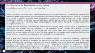
Groundwater replenishment is a critical factor for the augmentation and sustainability of water resources in the country. There is significant potential in both rural and urban areas for harvesting rainwater from individual rooftops. The Central Ground Water Board (CGWB) has published several scientific manuals and reports on rooftop rainwater harvesting (RTRWH) potential, as well as FAQs and practical guides for artificial recharge. However, there is currently no user-friendly digital platform where individuals can directly assess their rainwater harvesting potential.
Proposed Solution
To promote public participation in groundwater conservation, it is proposed to develop a web/mobile application that enables users to easily estimate the feasibility of rooftop rainwater harvesting (RTRWH) and artificial recharge at their locations. By entering simple details such as name, location, number of dwellers, roof area, and available open space, the system will generate personalized outputs using GIS-based and algorithmic models.
Key Features
- Feasibility check for rooftop rainwater harvesting
- Suggested type of RTRWH/Artificial Recharge structures
- Information on principal aquifer in the area
- Depth to groundwater level
- Local rainfall data
- Runoff generation capacity
- Recommended dimensions of recharge pits, trenches, and shafts
- Cost estimation and cost-benefit analysis
Impact
The application will empower individuals and communities to take informed decisions about groundwater conservation and rainwater harvesting. It will enhance public awareness, encourage participation, and support sustainable water management efforts. The tool should also support regional languages for better accessibility and inclusivity.
Give me the ye features to include in mvp for this project Designing and development of an application for on spot assessment of Roof Top Rain water harvesting and artificial recharge potential and size of the RTRWH and AR.
Background
Groundwater replenishment is a critical factor for the augmentation and sustainability of water resources in the country. There is significant potential in both rural and urban areas for harvesting rainwater from individual rooftops. The Central Ground Water Board (CGWB) has published several scientific manuals and reports on rooftop rainwater harvesting (RTRWH) potential, as well as FAQs and practical guides for artificial recharge. However, there is currently no user-friendly digital platform where individuals can directly assess their rainwater harvesting potential.
Proposed Solution
To promote public participation in groundwater conservation, it is proposed to develop a web/mobile application that enables users to easily estimate the feasibility of rooftop rainwater harvesting (RTRWH) and artificial recharge at the


![Forecast Accuracy Measures
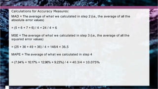
In this section, we will calculate forecast accuracy measures such as Mean Absolute
Deviation (MAD), Mean Squared Error (MSE), and Mean Absolute Percentage
Error (MAPE). We will explain the calculations using the next example.
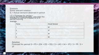
Example
The following actual demand and forecast values are given for the past four periods.
We want to calculate MAD, MSE and MAPE for this forecast to see how well it is doing.
Note that Abs (et) refers to the absolute value of the error in period t (et).
et
2 [Abs (et) / Dt] x 100%
Period Actual Demand Forecast et Abs (et)
1 63 68
2 59 65
3 54 61
4 65 59](https://image.slidesharecdn.com/demandforecasting-250925224223-6ac19572/85/Demand-Forecasrtqywyyevdhusisvdhisisting-pptx-29-320.jpg)
![Here are what need to do:
Step 1: Calculate the error as et = Dt – Ft (the difference between the actual demand and the
forecast) for any period t and enter the values in the table above.
Step 2: Calculate the absolute value of the errors calculated in step 1 [i.e., Abs (et)], and
enter the values in the table above.
t
Step 3: Calculate the squared error (i.e., e 2) for each period and enter the values in the table
Period Actual Demand Forecast et Abs (et) t
e 2
[Abs (et) / Dt] x
100%
1 63 68 -5 5 25 7.94%
2 59 65 -6 6 36 10.17%
3 54 61 -7 7 49 12.96%
4 65 59 6 6 36 9.23%
above.
Step 4: Calculate [Abs (et) / Dt] x 100% for each period and enter the value under its column
in the table above.
Solution](https://image.slidesharecdn.com/demandforecasting-250925224223-6ac19572/85/Demand-Forecasrtqywyyevdhusisvdhisisting-pptx-30-320.jpg)