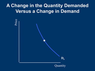
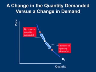
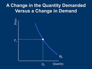
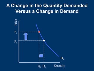
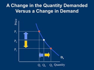
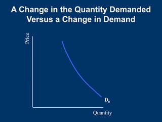
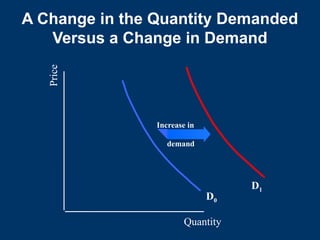
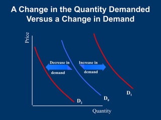
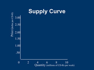
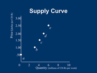
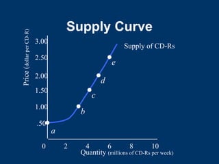
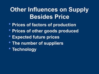
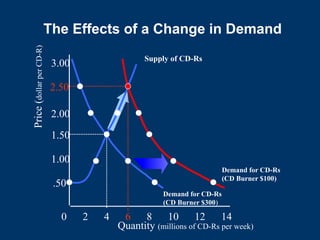
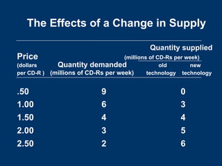
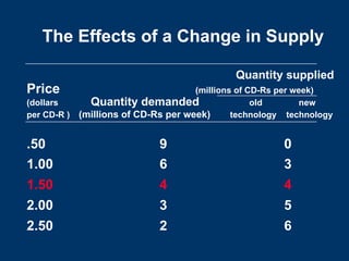
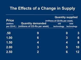
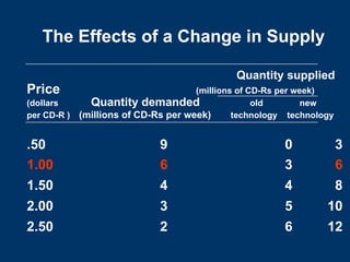
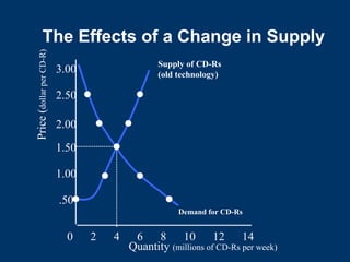
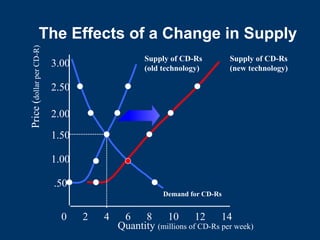
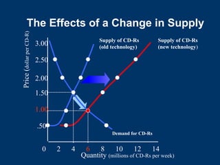
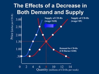
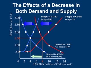
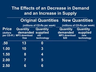
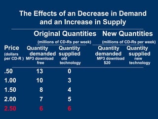
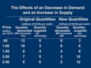
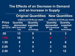
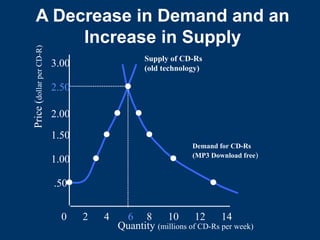
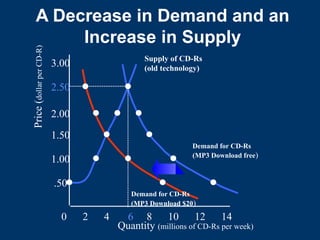
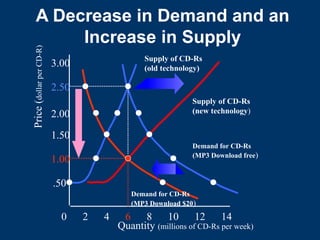
CHAPTER
3
Demand and
Supply
Chapter 3
Demand, Supply and
Relative Prices
 Demand and supply determine
relative prices.
 The word “price” means relative
price. Price is an opportunity cost.
 If we predict a price will fall, we mean
its price will fall relative to the
average price of other goods and
services.
Calculation of Relative
Prices
 Relative price is usually calculated
by dividing the price of a good in
question by a price index.
 The most commonly used price
index is the CPI (Consumer Price
Index).
 The CPI represents the “average”
price of consumer goods in a
particular month or year.
Demand
 The quantity demanded of a good or
service is the amount that
consumers plan to (or are willing to)
buy in a given period of time at a
particular (relative) price.
 Quantity demanded is measured as
an amount per unit time: pizzas per
day, pizzas per week, or pizzas per
year.
The Law of Demand
 Other things remaining the same, the
higher the price of a good, the
smaller is the quantity demanded.
 The phrase “other things being
equal” is sometimes abbreviated
with the Latin phrase ceteris paribus
(cet. par.).
 Thus, when we say price changes,
we mean relative price changes.
Demand Schedule
and Demand Curve
 A demand schedule lists the
quantities demanded at each
different price when all the other
influences on consumers’ planned
purchases remain the same.
 A demand curve is a graph of the
demand schedule.
Demand Schedule
a .50 9
b 1.00 6
c 1.50 4
d 2.00 3
e 2.50 2
Price Quantity Demanded
(dollars per CD-R) (millions of CD-Rs per week)
Demand Curve
0 2 4 6 8 10
.50
1.00
1.50
2.00
2.50
3.00
Quantity (millions of CD-Rs per week)
Price
(
dollar
per
CD-R)
Demand Curve
0 2 4 6 8 10
.50
1.00
1.50
2.00
2.50
3.00
Quantity (millions of CD-Rs per week)
Price
(
dollar
per
CD-R)
e
d
c
b
a
Demand Curve
0 2 4 6 8 10
.50
1.00
1.50
2.00
2.50
3.00
e
d
c
b
a
Demand
for CD-Rs
Quantity (millions of CD-Rs per week)
Price
(
dollar
per
CD-R)
Factors That
Influence Demand
 Price (of the good in question)
 Prices of related goods
 Income
 Expected future price
 Population
 Preferences (or Tastes)
Price
 If the price of the good rises, the
quantity demanded falls (a
movement up along the demand
curve).
 If the price of the good falls, the
quantity demanded rises (a
movement down along the demand
curve).
Prices of Related Goods
 A substitute is a good that can be used in
place of another good. If the price of a
CD-RW rises, the demand for CD-Rs rises
(demand curve shifts out to the right) .
 A complement is a good that is used in
conjunction with another good. If the
price of a CD burner rises, the demand for
CD-Rs falls (demand curve shifts in to the
left).
Example-Decrease in Price of a Complement
Original demand schedule New demand schedule
CD Burner $300 CD Burner $100
Price Quantity Price Quantity
(dollars (millions of CD-Rs (dollars (millions of CD-Rs
per CD-R) per week) per CD-R) per week))
a .50 9
b 1.00 6
c 1.50 4
d 2.00 3
e 2.50 2
Assume the original price of
A CD Burner is $300. The
demand schedule shows
the Price-Quantity
relationship for CD-Rs.
Example-Decrease in Price of a Complement
Original demand schedule New demand schedule
CD Burner $300 CD Burner $100
Price Quantity Price Quantity
(dollars (millions of CD-Rs (dollars (millions of CD-
Rs
per CD-R) per week) per CD-R) per week))
a .50 9 a’ .50 13
b 1.00 6 b’ 1.00 10
c 1.50 4 c’ 1.50 8
d 2.00 3 d’ 2.00 7
e 2.50 2 e’ 2.50 6
Demand Before Price of
Complement Decreases
0 2 4 6 8 10 12 14
.50
1.00
1.50
2.00
2.50
3.00
Quantity (millions of CD-Rs per week)
Price
(
dollar
per
CD-R)
e
d
c
b
a
Demand for CD-Rs
(CD Burner $300)
Demand after Price of
Complement Decreases
0 2 4 6 8 10 12 14
.50
1.00
1.50
2.00
2.50
3.00
e
d
c
b
a
Demand for CD-Rs
(CD Burner $300)
Quantity (millions of CD-Rs per week)
Price
(
dollar
per
CD-R)
e'
d'
c'
b'
a'
Demand for CD-Rs
(CD Burner $100)
Income
 Normal goods are those for which
demand increases as income
increases (demand curve shifts out
to the right).
 Inferior goods are those for which
demand decreases as income
increases (demand curve shifts in to
the left).
 The terms normal and inferior do not
necessarily refer to the quality of the
product
Expected Future Price
 If the price of a good is expected to
rise in the future and if the good can
be stored, people will often
substitute over time by buying more
of the good today.
 Demand for the good increases
(demand curve shifts out to the
right). This is sometimes called
speculation.
Population
 Other things remaining the same, the
larger the population, the greater is
the demand for all goods and
services (demand curve shifts out to
the right).
 The smaller the population, the
smaller is the demand for all goods
and services (demand curve shifts in
to the left).
Preferences (or Tastes)
 Preferences are an individual’s
attitudes toward goods and services.
 Different people have different
preferences and will therefore have
different demands for a particular
good or service.
Summary of Changes in
Demand
 Changes In Demand
– The demand for CD-Rs
• Decreases if:
– The price of a substitute falls
– The price of a complement rises
– Income falls (since CD-R is a normal good)
– The price of a CD-R is expected to fall in the future
– The population decreases
– Preferences decrease
Summary of Changes in
Demand
 Changes In Demand
– The demand for CD-Rs
• Increases if:
– The price of a substitute rises
– The price of a complement falls
– Income rises (since CD-R is a normal good)
– The price of a CD-R is expected to rise in the future
– The population increases
– Preferences increase
Movement Along Versus a
Shift of the Demand Curve
 If the price of a good changes but
everything else remains the same,
there is a movement along the
demand curve.
 If the price of a good remains
constant but some other influence on
buyers’ plans changes, there is a
shift of the demand curve.
A Change in Quantity
Demanded Versus a Change
in Demand
 A movement along the demand curve
shows a change in the quantity
demanded.
 A shift of the demand curve shows a
change in demand.
A Change in the Quantity Demanded
Versus a Change in Demand
Quantity
Price
D0
Quantity
Price
D0
Decrease in
quantity
demanded
Increase in
quantity
demanded
A Change in the Quantity Demanded
Versus a Change in Demand
Quantity
Price
D0
P0
Q0
A Change in the Quantity Demanded
Versus a Change in Demand
Quantity
Price
D0
P0
P1
Q0
Q1
A Change in the Quantity Demanded
Versus a Change in Demand
Quantity
Price
D0
P0
P2
P1
Q0 Q2
Q1
A Change in the Quantity Demanded
Versus a Change in Demand
Quantity
Price
D0
A Change in the Quantity Demanded
Versus a Change in Demand
Quantity
Price
D0
D1
Increase in
demand
A Change in the Quantity Demanded
Versus a Change in Demand
Price
Quantity
D0
D1
D2
Increase in
Decrease in
demand demand
A Change in the Quantity Demanded
Versus a Change in Demand
Quantity
Price
D0
D1
D2
D0
Decrease in
quantity
demanded
Increase in
quantity
demanded
Increase in
demand
Decrease in
demand
A Change in the Quantity Demanded
Versus a Change in Demand
Shift of Demand Versus Movement Along a
Demand Curve
• A change in demand is
not the same as a change
in quantity demanded.
• In this example, a higher
price causes lower
quantity demanded.
• Changes in determinants
of demand, other than
price, cause a change in
demand, or a shift of the
entire demand curve, from
DA to DB.
• When demand shifts to
the right, demand
increases. This causes
quantity demanded to be
greater than it was prior to
the shift, for each and
every price level.
A Change in Demand Versus a Change in
Quantity Demanded
A Change in Demand Versus a Change in
Quantity Demanded
To summarize:
Change in price of a good or service
leads to
Change in quantity demanded
(Movement along the curve).
Change in income, preferences, or
prices of other goods or services
leads to
Change in demand
(Shift of curve).
The Impact of a Change in
Income
• Higher income
decreases the demand
for an inferior good
• Higher income
increases the demand
for a normal good
The Impact of a Change in
the Price of Related Goods
• Price of hamburger rises
• Demand for complement good
(ketchup) shifts left
• Demand for substitute good (chicken)
shifts right
• Quantity of hamburger
demanded falls
From Household to Market
Demand
 Demand for a good or service can be
defined for an individual household, or
for a group of households that make
up a market.
 Market demand is the sum of all the
quantities of a good or service
demanded per period by all the
households buying in the market for
that good or service.
From Household Demand to
Market Demand
 Assuming there are only two
households in the market, market
demand is derived as follows:
42
Determinants of
Demand Elasticity
 Availability of substitutes
– The greater the availability of substitutes for a good, the greater the
good’s elasticity of demand
 Share of consumer’s budget spent on the good
– Increase in prices reduced the demand because people are not both
willing and able to purchase @ higher prices
 A matter of time
– The longer the adjustment period, the greater the consumer’s ability
to substitute
 Some elasticity estimates
– The elasticity of demand is greater in the long run because consumers
have more time to adjust
43
50 75 95100 Millions of gallons per day
0
$1.25
1.00
Price
per
gallon
Dy
Dm
Dw
Demand Becomes
More Elastic Over Time
4
Selected
Elasticities of Demand
Product Short Run Long Run
Electricity (residential) 0.1 1.9
Air travel 0.1 2.4
Medical care and hospitalization 0.3 0.9
Gasoline 0.4 1.5
Movies 0.9 3.7
Natural gas (residential) 1.4 2.1
45
Other Determinants of
Demand
Consumer Income
The prices of related goods
The number and composition of
consumers
Consumer expectations
Consumer tastes
46
Changes in Consumer
Income
 If income ↑, consumers willing and
able to buy more which ↑ demand
– Demand curve shifts to the right
 Two categories of goods:
– Normal goods – demand increases as money
income increases
– Inferior goods – demand decreases as money
income increases
• Examples: used clothing, bus rides, etc.
47
Changes in the Prices of
Related Goods
 Substitutes
– Decrease in price of one item will reduce the
demand for a substitute
• Example: Tacos and Pizza
 Complements
– Certain goods used together
• Example: airline tickets and car rentals
– A decrease in the price of one shifts the
demand of the other rightward
48
Changes in Prices of
Related Goods (cont)
 Changes in size or composition of the
population will increase demand and shift
the curve to the right
 Changes in consumer expectations can
shift the demand curve to the left or the
right
 Changes in consumer tastes
– Tastes are your likes and dislikes as a consumer
49
Movement along
the Curve
 Movement vs. Shift
– A change in price, causes a movement along
the demand curve, changes the quantity
demanded
– A change in one of the determinants of
demand other than price causes a shift of a
demand curve
Supply
 If a firm supplies a good or service,
the firm
– Has the resources and technology to produce it,
– Can profit from producing it, and
– Has made a definite plan to produce it and sell
it.
Supply
 The amount of a good or service that
producers plan to (or are willing to)
sell during a given time period at a
particular price is called the quantity
supplied.
 Quantity supplied is not necessarily
the same as the quantity actually
sold (which depends on the
interaction of supply and demand).
The Law of Supply
 Other things remaining the same, the
higher the price of a good, the
greater is the quantity supplied.
 Increasing opportunity cost is the
reason behind the law of supply.
Supply Schedule
and Supply Curve
 A supply schedule lists the
quantities supplied at each different
price when all other influences on
the amount firms plan to sell remain
the same.
 A supply curve is a graph of a supply
schedule.
Supply Schedule
a .50 0
b 1.00 3
c 1.50 4
d 2.00 5
e 2.50 6
Price Quantity
(dollars per CD-R) (millions of CD-Rs per week)
Supply Curve
Quantity (millions of CD-Rs per week)
0 2 4 6 8 10
.50
1.00
1.50
2.00
2.50
3.00
Price
(
dollar
per
CD-R)
Supply Curve
Quantity (millions of CD-Rs per week)
0 2 4 6 8 10
.50
1.00
1.50
2.00
2.50
3.00
Price
(
dollar
per
CD-R)
a
b
c
d
e
Supply Curve
0 2 4 6 8 10
.50
1.00
1.50
2.00
2.50
3.00
Quantity (millions of CD-Rs per week)
Price
(
dollar
per
CD-R)
Supply of CD-Rs
a
b
c
d
e
Other Influences on Supply
Besides Price
 Prices of factors of production
 Prices of other goods produced
 Expected future prices
 The number of suppliers
 Technology
Prices of Factors
of Production
 A change in the price of a factor of
production causes supply to change
by changing production costs.
 For example, suppose the product is
automobiles and the price of labor
increases. Automakers will cut back
on their supply (the supply curve will
shift to the left).
Prices of Related Goods
Produced - Substitutes
 Two goods are substitutes in
production if the same factors of
production can be used to produce
each good. Examples are sedans
and sports cars.
 If the price of sports cars rises, the
quantity supplied of sports cars rises
(move up the supply curve) and the
supply of sedans falls (the supply
curve of sedans shifts to the left).
Prices of Related Goods
Produced - Complements
 Two goods are complements in production
if they are produced together. Examples
are beef and cowhide.
 If the price of cowhide rises, the quantity
supplied of cowhide rises (move up along
the supply curve) and the supply of beef
rises (the supply curve of beef shifts to
the right).
Expected Future Prices
 If producers expect the price of a
good to be higher in the future (and
the good can be stored), they may
substitute over time.
 This means they will offer a smaller
quantity of the good for sale today so
the current supply decreases (the
supply curve shifts to the left) .
The Number of Suppliers
 Other things remaining the same, the
larger the number of producers
supplying a good, the larger is the
supply of the good (the supply curve
shifts to the right).
Technology
 New technologies that enable
producers to use less (or cheaper)
factors of production lower the cost
of production and increase supply
(the supply curve shifts to the right).
Supply Response to Change in Technology
Original supply schedule
Old technology
Price Quantity
(dollars (millions of CD-Rs
per CD-R) per week)
a .50 0
b 1.00 3
c 1.50 4
d 2.00 5
e 2.50 6
Original supply schedule New supply schedule
Old technology New technology
Price Quantity Price Quantity
(dollars (millions of CD-Rs (dollars (millions of CD-Rs
per CD-R) per week) per CD-R) per week)
a .50 0 a' .50
b 1.00 3 b' 1.00
c 1.50 4 c' 1.50
d 2.00 5 d' 2.00
e 2.50 6 e' 2.50
Supply Response to Change in Technology
Original supply schedule New supply
schedule
Old technology New
technology
Price Quantity Price
Quantity
(dollars (millions of CD-Rs (dollars (millions of CD-
Rs
per CD-R) per week) per CD-R) per week)
a .50 0 a' .50 3
b 1.00 3 b' 1.00 6
c 1.50 4 c' 1.50 8
d 2.00 5 d' 2.00 10
Supply Response to Change in Technology
Quantity (millions of CD-Rs per week)
0 2 4 6 8 10 12 14
.50
1.00
1.50
2.00
2.50
3.00
Price
(
dollar
per
CD-R)
Supply of CD-Rs
(old technology)
e
d
c
b
a
Supply Response to Change in Technology
Quantity (millions of CD-Rs per week)
Price
(
dollar
per
CD-R)
0 2 4 6 8 10 12 14
.50
1.00
1.50
2.00
2.50
3.00 Supply of CD-Rs
(new technology)
a a'
b'
c'
d'
e'
e
d
c
b
Supply of CD-Rs
(old technology)
Supply Response to Change in Technology
Movement Along Versus a
Shift of the Supply Curve
 If the price of a good changes but
everything else influencing supply
remains constant, there is a
movement along the supply curve.
 If the price of a good remains the
same but another influence on
supply changes, there is a shift of
the supply curve.
A Change in Quantity
Supplied Versus a Change
in Supply
 A movement along the supply curve
shows a change in quantity supplied.
 A shift of the supply curve shows a
change in supply.
A Change in the Quantity Supplied
Versus a Change in Supply
Quantity
Price
S0
A Change in the Quantity Supplied
Versus a Change in Supply
Quantity
Price
S0
Decrease in
quantity
supplied
Increase in
quantity
supplied
A Change in the Quantity Supplied
Versus a Change in Supply
Quantity
Price
S0
P0
Q0
A Change in the Quantity Supplied
Versus a Change in Supply
Quantity
Price
S0
P0
Q1
Q0
P1
A Change in the Quantity Supplied
Versus a Change in Supply
Quantity
Price
S0
P0
Q1
Q0
P1
P2
Q2
A Change in the Quantity Supplied
Versus a Change in Supply
Quantity
S1
Price
S0
supply
Increase in
A Change in the Quantity Supplied
Versus a Change in Supply
Quantity
S1
Price
S0
S2
supply
Increase in
Decrease in
supply
A Change in the Quantity Supplied
Versus a Change in Supply
Quantity
Price
S0
Decrease in
quantity
supplied
Increase in
quantity
supplied
S0 S1
S2
Increase in
supply
supply
Decrease in
Price Determination
 The price of a good regulates the
quantities demanded and supplied.
 There is one price, and only one
price, at which the quantity
demanded equals the quantity
supplied.
 Price is the rationing (or regulating)
mechanism
Shortages
 If the price is too low, the quantity
demanded exceeds the quantity
supplied. People are willing to pay
more for the good.
 To eliminate this shortage, sellers
will raise the price, increasing the
quantity supplied and reducing the
quantity demanded.
Surpluses
 If the price is too high, the quantity
supplied exceeds the quantity
demand. Inventories pile up.
 To eliminate this surplus, sellers will
lower the price, reducing quantity
supplied and increasing quantity
demanded.
Market Equilibrium
 The market equilibrium price is the
price at which the quantity
demanded equals the quantity
supplied.
 The market equilibrium quantity is
the quantity bought and sold at the
equilibrium price.
 At market equilibrium, both buyers
and sellers are satisfied. This is not
true at any other price or quantity.
Market Equilibrium
Quantity Quantity
Shortage(–)
Price demanded supplied or
surplus(+)
(dollars
per CD-R) (millions of CD-Rs per week)
.50 9 0
1.00 6 3
1.50 4 4
2.00 3 5
2.50 2 6
Market Equilibrium
Quantity Quantity
Shortage(–)
Price demanded supplied or surplus(+)
(dollars
per CD-R) (millions of CD-Rs per week)
.50 9 0
–9
1.00 6 3
1.50 4 4
2.00 3 5
2.50 2 6
Market Equilibrium
Quantity Quantity
Shortage(–)
Price demanded supplied or surplus(+)
(dollars
per CD-R) (millions of CD-Rs per week)
.50 9 0
–9
1.00 6 3
–3
1.50 4 4
2.00 3 5
Market Equilibrium
Quantity Quantity
Shortage(–)
Price demanded supplied or surplus(+)
(dollars
per CD-R) (millions of CD-Rs per week)
.50 9 0
–9
1.00 6 3
–3
1.50 4 4
0
Market Equilibrium
Quantity Quantity
Shortage(–)
Price demanded supplied or surplus(+)
(dollars
per CD-R) (millions of CD-Rs per week)
.50 9 0
–9
1.00 6 3
–3
1.50 4 4
0
Market Equilibrium
Quantity Quantity
Shortage(–)
Price demanded supplied or surplus(+)
(dollars
per CD-R) (millions of CD-Rs per week)
.50 9 0
–9
1.00 6 3
–3
1.50 4 4
0
Market Equilibrium
Quantity Quantity
Shortage(–)
Price demanded supplied or surplus(+)
(dollars
per CD-R) (millions of CD-Rs per week)
.50 9 0
–9
1.00 6 3
–3
1.50 4 4
0
Market Equilibrium
0 2 4 6 8 10
.50
1.00
1.50
2.00
2.50
3.00
Quantity (millions of CD-Rs per week)
Price
(
dollar
per
CD-R)
Market Equilibrium
0 2 4 6 8 10
.50
1.00
1.50
2.00
2.50
3.00
Quantity (millions of CD-Rs per week)
Price
(
dollar
per
CD-R)
Demand
for CD-Rs
Market Equilibrium
0 2 4 6 8 10
.50
1.00
1.50
2.00
2.50
3.00
Quantity (millions of CD-Rs per week)
Price
(
dollar
per
CD-R)
Supply of CD-Rs
Demand
for CD-Rs
Market Equilibrium
0 2 4 6 8 10
.50
1.00
1.50
2.00
2.50
3.00
Quantity (millions of CD-Rs per week)
Price
(
dollar
per
CD-R)
Supply of CD-Rs
Demand
for CD-Rs
A Shortage Forces
the Price Up
 If demand exceeds supply, sellers
will raise price, decreasing quantity
demanded.
A Surplus Forces
the Price Down
 If supply exceeds demand, sellers
will see their inventories of unsold
goods piling up and will cut price to
sell them.
Market Equilibrium
0 2 4 6 8 10
.50
1.00
1.50
2.00
2.50
3.00
Quantity (millions of CD-Rs per week)
Price
(
dollar
per
CD-R)
Supply of CD-Rs
Surplus of
2 million CD-Rs
at $2 a CD-R
Shortage of
3 million
CD-Rs at $1
a CD-R
Demand
for CD-Rs
Equilibrium
The Best Deal Available
for Buyers and Sellers
 The equilibrium price is the best deal
available for buyers and sellers.
 This is the price at which trade takes
place.
Predicting Changes in
Price and Quantity
 The theory we have just studied
provides us with a powerful way of
analyzing influences on prices and
the quantities bought and sold.
 A change in price must be caused by
either a change in demand or a
change in supply.
A Change in Demand
 An increase in demand shifts the
demand curve up and to the right.
 The new equilibrium price and
quantity are higher.
Predicting Changes in
Price and Quantity
 A Change in Demand
– What would happen to the price and quantity of
CD-Rs if the price of a CD Burner falls from
$300 to $100.
The Effects of a Change in
Demand
Quantity demanded
Price (millions of CD-Rs per week)
(dollars Quantity supplied
per CD-R ) CD Burner $300 CD Burner $100 (millions of CD-Rs per week)
.50 9 0
1.00 6 3
1.50 4 4
2.00 3 5
2.50 2 6
The Effects of a Change in
Demand
Quantity demanded
Price (millions of CD-Rs per week)
(dollars Quantity supplied
per CD-R ) CD Burner $300 CD Burner $100 (millions of CD-Rs per week)
.50 9 0
1.00 6 3
1.50 4 4
2.00 3 5
2.50 2 6
The Effects of a Change in
Demand
Quantity demanded
Price (millions of CD-Rs per week)
(dollars Quantity supplied
per CD-R ) CD Burner $300 CD Burner $100 (millions of CD-Rs per week)
.50 9 13 0
1.00 6 10 3
1.50 4 8 4
2.00 3 7 5
2.50 2 6 6
The Effects of a Change in
Demand
Quantity demanded
Price (millions of CD-Rs per week)
(dollars Quantity supplied
per CD-R ) CD Burner $300 CD Burner $100 (millions of CD-Rs per week)
.50 9 13 0
1.00 6 10 3
1.50 4 8 4
2.00 3 7 5
2.50 2 6 6
The Effects of a Change in Demand
Quantity (millions of CD-Rs per week)
0 2 4 6 8 10 12 14
.50
1.00
1.50
2.00
2.50
3.00
Price
(
dollar
per
CD-R)
Supply of CD-Rs
Demand for CD-Rs
(CD Burner $300)
The Effects of a Change in Demand
Quantity (millions of CD-Rs per week)
0 2 4 6 8 10 12 14
.50
1.00
1.50
2.00
2.50
3.00
Price
(
dollar
per
CD-R)
Supply of CD-Rs
Demand for CD-Rs
(CD Burner $300)
Demand for CD-Rs
(CD Burner $100)
The Effects of a Change in Demand
Quantity (millions of CD-Rs per week)
0 2 4 6 8 10 12 14
.50
1.00
1.50
2.00
2.50
3.00
Price
(
dollar
per
CD-R)
Supply of CD-Rs
Demand for CD-Rs
(CD Burner $300)
Demand for CD-Rs
(CD Burner $100)
A Change in Supply
 An increase in supply shifts the
supply curve down and to the right.
 The new equilibrium price is lower,
but the equilibrium quantity is higher.
The Effects of a Change in Supply
Quantity supplied
Price (millions of CD-Rs per week)
(dollars Quantity demanded old new
per CD-R ) (millions of CD-Rs per week) technology technology
.50 9 0
1.00 6 3
1.50 4 4
2.00 3 5
2.50 2 6
The Effects of a Change in Supply
Quantity supplied
Price (millions of CD-Rs per week)
(dollars Quantity demanded old new
per CD-R ) (millions of CD-Rs per week) technology technology
.50 9 0
1.00 6 3
1.50 4 4
2.00 3 5
2.50 2 6
Quantity supplied
Price (millions of CD-Rs per week)
(dollars Quantity demanded old new
per CD-R ) (millions of CD-Rs per week) technology technology
.50 9 0 3
1.00 6 3 6
1.50 4 4 8
2.00 3 5 10
2.50 2 6 12
The Effects of a Change in Supply
Quantity supplied
Price (millions of CD-Rs per week)
(dollars Quantity demanded old new
per CD-R ) (millions of CD-Rs per week) technology technology
.50 9 0 3
1.00 6 3 6
1.50 4 4 8
2.00 3 5 10
2.50 2 6 12
The Effects of a Change in Supply
Quantity (millions of CD-Rs per week)
0 2 4 6 8 10 12 14
.50
1.00
1.50
2.00
2.50
3.00
Price
(
dollar
per
CD-R)
Demand for CD-Rs
Supply of CD-Rs
(old technology)
The Effects of a Change in Supply
Quantity (millions of CD-Rs per week)
0 2 4 6 8 10 12 14
.50
1.00
1.50
2.00
2.50
3.00
Price
(
dollar
per
CD-R)
Supply of CD-Rs
(old technology)
Demand for CD-Rs
Supply of CD-Rs
(new technology)
The Effects of a Change in Supply
Quantity (millions of CD-Rs per week)
0 2 4 6 8 10 12 14
.50
1.00
1.50
2.00
2.50
3.00
Price
(
dollar
per
CD-R)
Supply of CD-Rs
(old technology)
Demand for CD-Rs
Supply of CD-Rs
(new technology)
The Effects of a Change in Supply
A Change in Both
Demand and Supply
 Both curves shift.
 The direction in which price and
quantity change will depend on how
each curve shifts.
Demand and Supply Change
in the Same Direction
 If demand and supply increase, both
the demand and supply curves shift
out.
 The new equilibrium quantity will be
higher.
 The new equilibrium price may be
higher, lower, or it may remain the
same.
The Effects of an Increase in
Both Demand and Supply
Original Quantities New Quantities
(millions of CD-Rs per week) (millions of CD-Rs per
week)
Price Quantity Quantity Quantity Quantity
(dollars demanded supplied demanded supplied
per CD-R ) CD Burner old CD Burner new
$300 technology $100 technology
.50 9 0
1.00 6 3
1.50 4 4
2.00 3 5
2.50 2 6
The Effects of an Increase in
Both Demand and Supply
Original Quantities New Quantities
(millions of CD-Rs per week) (millions of CD-Rs per
week)
Price Quantity Quantity Quantity Quantity
(dollars demanded supplied demanded supplied
per CD-R ) CD Burner old CD Burner new
$300 technology $100 technology
.50 9 0 13 3
1.00 6 3 10 6
1.50 4 4 8 8
2.00 3 5 7 10
2.50 2 6 6 12
The Effects of an Increase in
Both Demand and Supply
Quantity (millions of CD-Rs per week)
0 2 4 6 8 10 12 14
.50
1.00
1.50
2.00
2.50
3.00
Price
(
dollar
per
CD-R)
Supply of CD-Rs
(old technology)
Demand for CD-Rs
(CD Burner $300)
The Effects of an Increase in
Both Demand and Supply
Quantity (millions of CD-Rs per week)
0 2 4 6 8 10 12 14
.50
1.00
1.50
2.00
2.50
3.00
Price
(
dollar
per
CD-R)
Supply of CD-Rs
(old technology)
Demand for CD-Rs
(CD Burner $300)
Demand for CD-Rs
(CD Burner $100)
The Effects of an Increase in
Both Demand and Supply
Quantity (millions of CD-Rs per week)
0 2 4 6 8 10 12 14
.50
1.00
1.50
2.00
2.50
3.00
Price
(
dollar
per
CD-R)
Supply of CD-Rs
(old technology)
Demand for CD-Rs
(CD Burner $300)
Demand for CD-Rs
(CD Burner $100)
Supply of CD-Rs
(new technology)
A Decrease in Both
Demand and Supply
 When both demand and supply
decrease, the quantity decreases and
the price increases, decreases, or
remains constant
The Effects of a Decrease in
Both Demand and Supply
Quantity (millions of CD-Rs per week)
0 2 4 6 8 10 12 14
.50
1.00
1.50
2.00
2.50
3.00
Price
(
dollar
per
CD-R)
Demand for CD-Rs
(CD Burner $100)
Supply of CD-Rs
(wage=$9)
The Effects of a Decrease in
Both Demand and Supply
Quantity (millions of CD-Rs per week)
0 2 4 6 8 10 12 14
.50
1.00
1.50
2.00
2.50
3.00
Price
(
dollar
per
CD-R)
Supply of CD-Rs
(wage=$10)
Demand for CD-Rs
(CD Burner $100)
Supply of CD-Rs
(wage=$9)
The Effects of a Decrease in
Both Demand and Supply
Quantity (millions of CD-Rs per week)
0 2 4 6 8 10 12 14
.50
1.00
1.50
2.00
2.50
3.00
Price
(
dollar
per
CD-R)
Supply of CD-Rs
(wage=$10)
Demand for CD-Rs
(CD Burner $300)
Demand for CD-Rs
(CD Burner $100)
Supply of CD-Rs
(wage=$9)
Demand and Supply Change
in Opposite Directions
 Suppose supply increases but
demand decreases.
 Price falls.
 The direction in which quantity
changes will depend on the
magnitude of the shifts in the two
curves.
The Effects of an Decrease in Demand
and an Increase in Supply
Original Quantities New Quantities
(millions of CD-Rs per week) (millions of CD-Rs per week)
Price Quantity Quantity Quantity Quantity
(dollars demanded supplied demanded supplied
per CD-R ) MP3 download old MP3 download new
free technology $20 technology
.50 13 0
1.00 10 3
1.50 8 4
2.00 7 5
2.50 6 6
The Effects of an Decrease in Demand
and an Increase in Supply
Original Quantities New Quantities
(millions of CD-Rs per week) (millions of CD-Rs per week)
Price Quantity Quantity Quantity Quantity
(dollars demanded supplied demanded supplied
per CD-R ) MP3 download old MP3 download new
free technology $20 technology
.50 13 0 9 3
1.00 10 3 6 6
1.50 8 4 4 8
2.00 7 5 3 10
2.50 6 6 2 12
A Decrease in Demand and an
Increase in Supply
Quantity (millions of CD-Rs per week)
0 2 4 6 8 10 12 14
.50
1.00
1.50
2.00
2.50
3.00
Price
(
dollar
per
CD-R)
Supply of CD-Rs
(old technology)
Demand for CD-Rs
(MP3 Download free)
A Decrease in Demand and an
Increase in Supply
Quantity (millions of CD-Rs per week)
0 2 4 6 8 10 12 14
.50
1.00
1.50
2.00
2.50
3.00
Price
(
dollar
per
CD-R)
Supply of CD-Rs
(old technology)
Demand for CD-Rs
(MP3 Download free)
Demand for CD-Rs
(MP3 Download $20)
A Decrease in Demand and an
Increase in Supply
Quantity (millions of CD-Rs per week)
0 2 4 6 8 10 12 14
.50
1.00
1.50
2.00
2.50
3.00
Price
(
dollar
per
CD-R)
Supply of CD-Rs
(old technology)
Demand for CD-Rs
(MP3 Download free)
Demand for CD-Rs
(MP3 Download $20)
Supply of CD-Rs
(new technology)
The Effects of an Increase in
Demand and a Decrease in
Supply
 When demand increases and supply
decreases, the price rises and the
quantity increases, decreases, or
remains constant.
An Increase in Demand and a
Decrease in Supply
Quantity (millions of CD-Rs per week)
0 2 4 6 8 10 12 14
.50
1.00
1.50
2.00
2.50
3.00
Price
(
dollar
per
CD-R)
Demand for CD-Rs
(MP3 download $20)
Supply of CD-Rs
(wage=$9)
An Increase in Demand and a
Decrease in Supply
Quantity (millions of CD-Rs per week)
0 2 4 6 8 10 12 14
.50
1.00
1.50
2.00
2.50
3.00
Price
(
dollar
per
CD-R)
Demand for CD-Rs
(MP3 download free)
Demand for CD-Rs
(MP3 download $20)
Supply of CD-Rs
(wage=$9)
An Increase in Demand and a
Decrease in Supply
Quantity (millions of CD-Rs per week)
0 2 4 6 8 10 12 14
.50
1.00
1.50
2.00
2.50
3.00
Price
(
dollar
per
CD-R)
Supply of CD-Rs
(wage=$10)
Demand for CD-Rs
(MP3 download free)
Demand for CD-Rs
(MP3 download $20)
Supply of CD-Rs
(wage=$9)

Demand and supplies class 11 topic .pptx

  • 1.
  • 2.
    Chapter 3 Demand, Supplyand Relative Prices  Demand and supply determine relative prices.  The word “price” means relative price. Price is an opportunity cost.  If we predict a price will fall, we mean its price will fall relative to the average price of other goods and services.
  • 3.
    Calculation of Relative Prices Relative price is usually calculated by dividing the price of a good in question by a price index.  The most commonly used price index is the CPI (Consumer Price Index).  The CPI represents the “average” price of consumer goods in a particular month or year.
  • 4.
    Demand  The quantitydemanded of a good or service is the amount that consumers plan to (or are willing to) buy in a given period of time at a particular (relative) price.  Quantity demanded is measured as an amount per unit time: pizzas per day, pizzas per week, or pizzas per year.
  • 5.
    The Law ofDemand  Other things remaining the same, the higher the price of a good, the smaller is the quantity demanded.  The phrase “other things being equal” is sometimes abbreviated with the Latin phrase ceteris paribus (cet. par.).  Thus, when we say price changes, we mean relative price changes.
  • 6.
    Demand Schedule and DemandCurve  A demand schedule lists the quantities demanded at each different price when all the other influences on consumers’ planned purchases remain the same.  A demand curve is a graph of the demand schedule.
  • 7.
    Demand Schedule a .509 b 1.00 6 c 1.50 4 d 2.00 3 e 2.50 2 Price Quantity Demanded (dollars per CD-R) (millions of CD-Rs per week)
  • 8.
    Demand Curve 0 24 6 8 10 .50 1.00 1.50 2.00 2.50 3.00 Quantity (millions of CD-Rs per week) Price ( dollar per CD-R)
  • 9.
    Demand Curve 0 24 6 8 10 .50 1.00 1.50 2.00 2.50 3.00 Quantity (millions of CD-Rs per week) Price ( dollar per CD-R) e d c b a
  • 10.
    Demand Curve 0 24 6 8 10 .50 1.00 1.50 2.00 2.50 3.00 e d c b a Demand for CD-Rs Quantity (millions of CD-Rs per week) Price ( dollar per CD-R)
  • 11.
    Factors That Influence Demand Price (of the good in question)  Prices of related goods  Income  Expected future price  Population  Preferences (or Tastes)
  • 12.
    Price  If theprice of the good rises, the quantity demanded falls (a movement up along the demand curve).  If the price of the good falls, the quantity demanded rises (a movement down along the demand curve).
  • 13.
    Prices of RelatedGoods  A substitute is a good that can be used in place of another good. If the price of a CD-RW rises, the demand for CD-Rs rises (demand curve shifts out to the right) .  A complement is a good that is used in conjunction with another good. If the price of a CD burner rises, the demand for CD-Rs falls (demand curve shifts in to the left).
  • 14.
    Example-Decrease in Priceof a Complement Original demand schedule New demand schedule CD Burner $300 CD Burner $100 Price Quantity Price Quantity (dollars (millions of CD-Rs (dollars (millions of CD-Rs per CD-R) per week) per CD-R) per week)) a .50 9 b 1.00 6 c 1.50 4 d 2.00 3 e 2.50 2 Assume the original price of A CD Burner is $300. The demand schedule shows the Price-Quantity relationship for CD-Rs.
  • 15.
    Example-Decrease in Priceof a Complement Original demand schedule New demand schedule CD Burner $300 CD Burner $100 Price Quantity Price Quantity (dollars (millions of CD-Rs (dollars (millions of CD- Rs per CD-R) per week) per CD-R) per week)) a .50 9 a’ .50 13 b 1.00 6 b’ 1.00 10 c 1.50 4 c’ 1.50 8 d 2.00 3 d’ 2.00 7 e 2.50 2 e’ 2.50 6
  • 16.
    Demand Before Priceof Complement Decreases 0 2 4 6 8 10 12 14 .50 1.00 1.50 2.00 2.50 3.00 Quantity (millions of CD-Rs per week) Price ( dollar per CD-R) e d c b a Demand for CD-Rs (CD Burner $300)
  • 17.
    Demand after Priceof Complement Decreases 0 2 4 6 8 10 12 14 .50 1.00 1.50 2.00 2.50 3.00 e d c b a Demand for CD-Rs (CD Burner $300) Quantity (millions of CD-Rs per week) Price ( dollar per CD-R) e' d' c' b' a' Demand for CD-Rs (CD Burner $100)
  • 18.
    Income  Normal goodsare those for which demand increases as income increases (demand curve shifts out to the right).  Inferior goods are those for which demand decreases as income increases (demand curve shifts in to the left).  The terms normal and inferior do not necessarily refer to the quality of the product
  • 19.
    Expected Future Price If the price of a good is expected to rise in the future and if the good can be stored, people will often substitute over time by buying more of the good today.  Demand for the good increases (demand curve shifts out to the right). This is sometimes called speculation.
  • 20.
    Population  Other thingsremaining the same, the larger the population, the greater is the demand for all goods and services (demand curve shifts out to the right).  The smaller the population, the smaller is the demand for all goods and services (demand curve shifts in to the left).
  • 21.
    Preferences (or Tastes) Preferences are an individual’s attitudes toward goods and services.  Different people have different preferences and will therefore have different demands for a particular good or service.
  • 22.
    Summary of Changesin Demand  Changes In Demand – The demand for CD-Rs • Decreases if: – The price of a substitute falls – The price of a complement rises – Income falls (since CD-R is a normal good) – The price of a CD-R is expected to fall in the future – The population decreases – Preferences decrease
  • 23.
    Summary of Changesin Demand  Changes In Demand – The demand for CD-Rs • Increases if: – The price of a substitute rises – The price of a complement falls – Income rises (since CD-R is a normal good) – The price of a CD-R is expected to rise in the future – The population increases – Preferences increase
  • 24.
    Movement Along Versusa Shift of the Demand Curve  If the price of a good changes but everything else remains the same, there is a movement along the demand curve.  If the price of a good remains constant but some other influence on buyers’ plans changes, there is a shift of the demand curve.
  • 25.
    A Change inQuantity Demanded Versus a Change in Demand  A movement along the demand curve shows a change in the quantity demanded.  A shift of the demand curve shows a change in demand.
  • 26.
    A Change inthe Quantity Demanded Versus a Change in Demand Quantity Price D0
  • 27.
    Quantity Price D0 Decrease in quantity demanded Increase in quantity demanded AChange in the Quantity Demanded Versus a Change in Demand
  • 28.
    Quantity Price D0 P0 Q0 A Change inthe Quantity Demanded Versus a Change in Demand
  • 29.
    Quantity Price D0 P0 P1 Q0 Q1 A Change inthe Quantity Demanded Versus a Change in Demand
  • 30.
    Quantity Price D0 P0 P2 P1 Q0 Q2 Q1 A Changein the Quantity Demanded Versus a Change in Demand
  • 31.
    Quantity Price D0 A Change inthe Quantity Demanded Versus a Change in Demand
  • 32.
    Quantity Price D0 D1 Increase in demand A Changein the Quantity Demanded Versus a Change in Demand
  • 33.
    Price Quantity D0 D1 D2 Increase in Decrease in demanddemand A Change in the Quantity Demanded Versus a Change in Demand
  • 34.
    Quantity Price D0 D1 D2 D0 Decrease in quantity demanded Increase in quantity demanded Increasein demand Decrease in demand A Change in the Quantity Demanded Versus a Change in Demand
  • 35.
    Shift of DemandVersus Movement Along a Demand Curve • A change in demand is not the same as a change in quantity demanded. • In this example, a higher price causes lower quantity demanded. • Changes in determinants of demand, other than price, cause a change in demand, or a shift of the entire demand curve, from DA to DB.
  • 36.
    • When demandshifts to the right, demand increases. This causes quantity demanded to be greater than it was prior to the shift, for each and every price level. A Change in Demand Versus a Change in Quantity Demanded
  • 37.
    A Change inDemand Versus a Change in Quantity Demanded To summarize: Change in price of a good or service leads to Change in quantity demanded (Movement along the curve). Change in income, preferences, or prices of other goods or services leads to Change in demand (Shift of curve).
  • 38.
    The Impact ofa Change in Income • Higher income decreases the demand for an inferior good • Higher income increases the demand for a normal good
  • 39.
    The Impact ofa Change in the Price of Related Goods • Price of hamburger rises • Demand for complement good (ketchup) shifts left • Demand for substitute good (chicken) shifts right • Quantity of hamburger demanded falls
  • 40.
    From Household toMarket Demand  Demand for a good or service can be defined for an individual household, or for a group of households that make up a market.  Market demand is the sum of all the quantities of a good or service demanded per period by all the households buying in the market for that good or service.
  • 41.
    From Household Demandto Market Demand  Assuming there are only two households in the market, market demand is derived as follows:
  • 42.
    42 Determinants of Demand Elasticity Availability of substitutes – The greater the availability of substitutes for a good, the greater the good’s elasticity of demand  Share of consumer’s budget spent on the good – Increase in prices reduced the demand because people are not both willing and able to purchase @ higher prices  A matter of time – The longer the adjustment period, the greater the consumer’s ability to substitute  Some elasticity estimates – The elasticity of demand is greater in the long run because consumers have more time to adjust
  • 43.
    43 50 75 95100Millions of gallons per day 0 $1.25 1.00 Price per gallon Dy Dm Dw Demand Becomes More Elastic Over Time
  • 44.
    4 Selected Elasticities of Demand ProductShort Run Long Run Electricity (residential) 0.1 1.9 Air travel 0.1 2.4 Medical care and hospitalization 0.3 0.9 Gasoline 0.4 1.5 Movies 0.9 3.7 Natural gas (residential) 1.4 2.1
  • 45.
    45 Other Determinants of Demand ConsumerIncome The prices of related goods The number and composition of consumers Consumer expectations Consumer tastes
  • 46.
    46 Changes in Consumer Income If income ↑, consumers willing and able to buy more which ↑ demand – Demand curve shifts to the right  Two categories of goods: – Normal goods – demand increases as money income increases – Inferior goods – demand decreases as money income increases • Examples: used clothing, bus rides, etc.
  • 47.
    47 Changes in thePrices of Related Goods  Substitutes – Decrease in price of one item will reduce the demand for a substitute • Example: Tacos and Pizza  Complements – Certain goods used together • Example: airline tickets and car rentals – A decrease in the price of one shifts the demand of the other rightward
  • 48.
    48 Changes in Pricesof Related Goods (cont)  Changes in size or composition of the population will increase demand and shift the curve to the right  Changes in consumer expectations can shift the demand curve to the left or the right  Changes in consumer tastes – Tastes are your likes and dislikes as a consumer
  • 49.
    49 Movement along the Curve Movement vs. Shift – A change in price, causes a movement along the demand curve, changes the quantity demanded – A change in one of the determinants of demand other than price causes a shift of a demand curve
  • 51.
    Supply  If afirm supplies a good or service, the firm – Has the resources and technology to produce it, – Can profit from producing it, and – Has made a definite plan to produce it and sell it.
  • 52.
    Supply  The amountof a good or service that producers plan to (or are willing to) sell during a given time period at a particular price is called the quantity supplied.  Quantity supplied is not necessarily the same as the quantity actually sold (which depends on the interaction of supply and demand).
  • 53.
    The Law ofSupply  Other things remaining the same, the higher the price of a good, the greater is the quantity supplied.  Increasing opportunity cost is the reason behind the law of supply.
  • 54.
    Supply Schedule and SupplyCurve  A supply schedule lists the quantities supplied at each different price when all other influences on the amount firms plan to sell remain the same.  A supply curve is a graph of a supply schedule.
  • 55.
    Supply Schedule a .500 b 1.00 3 c 1.50 4 d 2.00 5 e 2.50 6 Price Quantity (dollars per CD-R) (millions of CD-Rs per week)
  • 56.
    Supply Curve Quantity (millionsof CD-Rs per week) 0 2 4 6 8 10 .50 1.00 1.50 2.00 2.50 3.00 Price ( dollar per CD-R)
  • 57.
    Supply Curve Quantity (millionsof CD-Rs per week) 0 2 4 6 8 10 .50 1.00 1.50 2.00 2.50 3.00 Price ( dollar per CD-R) a b c d e
  • 58.
    Supply Curve 0 24 6 8 10 .50 1.00 1.50 2.00 2.50 3.00 Quantity (millions of CD-Rs per week) Price ( dollar per CD-R) Supply of CD-Rs a b c d e
  • 59.
    Other Influences onSupply Besides Price  Prices of factors of production  Prices of other goods produced  Expected future prices  The number of suppliers  Technology
  • 60.
    Prices of Factors ofProduction  A change in the price of a factor of production causes supply to change by changing production costs.  For example, suppose the product is automobiles and the price of labor increases. Automakers will cut back on their supply (the supply curve will shift to the left).
  • 61.
    Prices of RelatedGoods Produced - Substitutes  Two goods are substitutes in production if the same factors of production can be used to produce each good. Examples are sedans and sports cars.  If the price of sports cars rises, the quantity supplied of sports cars rises (move up the supply curve) and the supply of sedans falls (the supply curve of sedans shifts to the left).
  • 62.
    Prices of RelatedGoods Produced - Complements  Two goods are complements in production if they are produced together. Examples are beef and cowhide.  If the price of cowhide rises, the quantity supplied of cowhide rises (move up along the supply curve) and the supply of beef rises (the supply curve of beef shifts to the right).
  • 63.
    Expected Future Prices If producers expect the price of a good to be higher in the future (and the good can be stored), they may substitute over time.  This means they will offer a smaller quantity of the good for sale today so the current supply decreases (the supply curve shifts to the left) .
  • 64.
    The Number ofSuppliers  Other things remaining the same, the larger the number of producers supplying a good, the larger is the supply of the good (the supply curve shifts to the right).
  • 65.
    Technology  New technologiesthat enable producers to use less (or cheaper) factors of production lower the cost of production and increase supply (the supply curve shifts to the right).
  • 66.
    Supply Response toChange in Technology Original supply schedule Old technology Price Quantity (dollars (millions of CD-Rs per CD-R) per week) a .50 0 b 1.00 3 c 1.50 4 d 2.00 5 e 2.50 6
  • 67.
    Original supply scheduleNew supply schedule Old technology New technology Price Quantity Price Quantity (dollars (millions of CD-Rs (dollars (millions of CD-Rs per CD-R) per week) per CD-R) per week) a .50 0 a' .50 b 1.00 3 b' 1.00 c 1.50 4 c' 1.50 d 2.00 5 d' 2.00 e 2.50 6 e' 2.50 Supply Response to Change in Technology
  • 68.
    Original supply scheduleNew supply schedule Old technology New technology Price Quantity Price Quantity (dollars (millions of CD-Rs (dollars (millions of CD- Rs per CD-R) per week) per CD-R) per week) a .50 0 a' .50 3 b 1.00 3 b' 1.00 6 c 1.50 4 c' 1.50 8 d 2.00 5 d' 2.00 10 Supply Response to Change in Technology
  • 69.
    Quantity (millions ofCD-Rs per week) 0 2 4 6 8 10 12 14 .50 1.00 1.50 2.00 2.50 3.00 Price ( dollar per CD-R) Supply of CD-Rs (old technology) e d c b a Supply Response to Change in Technology
  • 70.
    Quantity (millions ofCD-Rs per week) Price ( dollar per CD-R) 0 2 4 6 8 10 12 14 .50 1.00 1.50 2.00 2.50 3.00 Supply of CD-Rs (new technology) a a' b' c' d' e' e d c b Supply of CD-Rs (old technology) Supply Response to Change in Technology
  • 71.
    Movement Along Versusa Shift of the Supply Curve  If the price of a good changes but everything else influencing supply remains constant, there is a movement along the supply curve.  If the price of a good remains the same but another influence on supply changes, there is a shift of the supply curve.
  • 72.
    A Change inQuantity Supplied Versus a Change in Supply  A movement along the supply curve shows a change in quantity supplied.  A shift of the supply curve shows a change in supply.
  • 73.
    A Change inthe Quantity Supplied Versus a Change in Supply Quantity Price S0
  • 74.
    A Change inthe Quantity Supplied Versus a Change in Supply Quantity Price S0 Decrease in quantity supplied Increase in quantity supplied
  • 75.
    A Change inthe Quantity Supplied Versus a Change in Supply Quantity Price S0 P0 Q0
  • 76.
    A Change inthe Quantity Supplied Versus a Change in Supply Quantity Price S0 P0 Q1 Q0 P1
  • 77.
    A Change inthe Quantity Supplied Versus a Change in Supply Quantity Price S0 P0 Q1 Q0 P1 P2 Q2
  • 78.
    A Change inthe Quantity Supplied Versus a Change in Supply Quantity S1 Price S0 supply Increase in
  • 79.
    A Change inthe Quantity Supplied Versus a Change in Supply Quantity S1 Price S0 S2 supply Increase in Decrease in supply
  • 80.
    A Change inthe Quantity Supplied Versus a Change in Supply Quantity Price S0 Decrease in quantity supplied Increase in quantity supplied S0 S1 S2 Increase in supply supply Decrease in
  • 81.
    Price Determination  Theprice of a good regulates the quantities demanded and supplied.  There is one price, and only one price, at which the quantity demanded equals the quantity supplied.  Price is the rationing (or regulating) mechanism
  • 82.
    Shortages  If theprice is too low, the quantity demanded exceeds the quantity supplied. People are willing to pay more for the good.  To eliminate this shortage, sellers will raise the price, increasing the quantity supplied and reducing the quantity demanded.
  • 83.
    Surpluses  If theprice is too high, the quantity supplied exceeds the quantity demand. Inventories pile up.  To eliminate this surplus, sellers will lower the price, reducing quantity supplied and increasing quantity demanded.
  • 84.
    Market Equilibrium  Themarket equilibrium price is the price at which the quantity demanded equals the quantity supplied.  The market equilibrium quantity is the quantity bought and sold at the equilibrium price.  At market equilibrium, both buyers and sellers are satisfied. This is not true at any other price or quantity.
  • 85.
    Market Equilibrium Quantity Quantity Shortage(–) Pricedemanded supplied or surplus(+) (dollars per CD-R) (millions of CD-Rs per week) .50 9 0 1.00 6 3 1.50 4 4 2.00 3 5 2.50 2 6
  • 86.
    Market Equilibrium Quantity Quantity Shortage(–) Pricedemanded supplied or surplus(+) (dollars per CD-R) (millions of CD-Rs per week) .50 9 0 –9 1.00 6 3 1.50 4 4 2.00 3 5 2.50 2 6
  • 87.
    Market Equilibrium Quantity Quantity Shortage(–) Pricedemanded supplied or surplus(+) (dollars per CD-R) (millions of CD-Rs per week) .50 9 0 –9 1.00 6 3 –3 1.50 4 4 2.00 3 5
  • 88.
    Market Equilibrium Quantity Quantity Shortage(–) Pricedemanded supplied or surplus(+) (dollars per CD-R) (millions of CD-Rs per week) .50 9 0 –9 1.00 6 3 –3 1.50 4 4 0
  • 89.
    Market Equilibrium Quantity Quantity Shortage(–) Pricedemanded supplied or surplus(+) (dollars per CD-R) (millions of CD-Rs per week) .50 9 0 –9 1.00 6 3 –3 1.50 4 4 0
  • 90.
    Market Equilibrium Quantity Quantity Shortage(–) Pricedemanded supplied or surplus(+) (dollars per CD-R) (millions of CD-Rs per week) .50 9 0 –9 1.00 6 3 –3 1.50 4 4 0
  • 91.
    Market Equilibrium Quantity Quantity Shortage(–) Pricedemanded supplied or surplus(+) (dollars per CD-R) (millions of CD-Rs per week) .50 9 0 –9 1.00 6 3 –3 1.50 4 4 0
  • 92.
    Market Equilibrium 0 24 6 8 10 .50 1.00 1.50 2.00 2.50 3.00 Quantity (millions of CD-Rs per week) Price ( dollar per CD-R)
  • 93.
    Market Equilibrium 0 24 6 8 10 .50 1.00 1.50 2.00 2.50 3.00 Quantity (millions of CD-Rs per week) Price ( dollar per CD-R) Demand for CD-Rs
  • 94.
    Market Equilibrium 0 24 6 8 10 .50 1.00 1.50 2.00 2.50 3.00 Quantity (millions of CD-Rs per week) Price ( dollar per CD-R) Supply of CD-Rs Demand for CD-Rs
  • 95.
    Market Equilibrium 0 24 6 8 10 .50 1.00 1.50 2.00 2.50 3.00 Quantity (millions of CD-Rs per week) Price ( dollar per CD-R) Supply of CD-Rs Demand for CD-Rs
  • 96.
    A Shortage Forces thePrice Up  If demand exceeds supply, sellers will raise price, decreasing quantity demanded.
  • 97.
    A Surplus Forces thePrice Down  If supply exceeds demand, sellers will see their inventories of unsold goods piling up and will cut price to sell them.
  • 98.
    Market Equilibrium 0 24 6 8 10 .50 1.00 1.50 2.00 2.50 3.00 Quantity (millions of CD-Rs per week) Price ( dollar per CD-R) Supply of CD-Rs Surplus of 2 million CD-Rs at $2 a CD-R Shortage of 3 million CD-Rs at $1 a CD-R Demand for CD-Rs Equilibrium
  • 99.
    The Best DealAvailable for Buyers and Sellers  The equilibrium price is the best deal available for buyers and sellers.  This is the price at which trade takes place.
  • 100.
    Predicting Changes in Priceand Quantity  The theory we have just studied provides us with a powerful way of analyzing influences on prices and the quantities bought and sold.  A change in price must be caused by either a change in demand or a change in supply.
  • 101.
    A Change inDemand  An increase in demand shifts the demand curve up and to the right.  The new equilibrium price and quantity are higher.
  • 102.
    Predicting Changes in Priceand Quantity  A Change in Demand – What would happen to the price and quantity of CD-Rs if the price of a CD Burner falls from $300 to $100.
  • 103.
    The Effects ofa Change in Demand Quantity demanded Price (millions of CD-Rs per week) (dollars Quantity supplied per CD-R ) CD Burner $300 CD Burner $100 (millions of CD-Rs per week) .50 9 0 1.00 6 3 1.50 4 4 2.00 3 5 2.50 2 6
  • 104.
    The Effects ofa Change in Demand Quantity demanded Price (millions of CD-Rs per week) (dollars Quantity supplied per CD-R ) CD Burner $300 CD Burner $100 (millions of CD-Rs per week) .50 9 0 1.00 6 3 1.50 4 4 2.00 3 5 2.50 2 6
  • 105.
    The Effects ofa Change in Demand Quantity demanded Price (millions of CD-Rs per week) (dollars Quantity supplied per CD-R ) CD Burner $300 CD Burner $100 (millions of CD-Rs per week) .50 9 13 0 1.00 6 10 3 1.50 4 8 4 2.00 3 7 5 2.50 2 6 6
  • 106.
    The Effects ofa Change in Demand Quantity demanded Price (millions of CD-Rs per week) (dollars Quantity supplied per CD-R ) CD Burner $300 CD Burner $100 (millions of CD-Rs per week) .50 9 13 0 1.00 6 10 3 1.50 4 8 4 2.00 3 7 5 2.50 2 6 6
  • 107.
    The Effects ofa Change in Demand Quantity (millions of CD-Rs per week) 0 2 4 6 8 10 12 14 .50 1.00 1.50 2.00 2.50 3.00 Price ( dollar per CD-R) Supply of CD-Rs Demand for CD-Rs (CD Burner $300)
  • 108.
    The Effects ofa Change in Demand Quantity (millions of CD-Rs per week) 0 2 4 6 8 10 12 14 .50 1.00 1.50 2.00 2.50 3.00 Price ( dollar per CD-R) Supply of CD-Rs Demand for CD-Rs (CD Burner $300) Demand for CD-Rs (CD Burner $100)
  • 109.
    The Effects ofa Change in Demand Quantity (millions of CD-Rs per week) 0 2 4 6 8 10 12 14 .50 1.00 1.50 2.00 2.50 3.00 Price ( dollar per CD-R) Supply of CD-Rs Demand for CD-Rs (CD Burner $300) Demand for CD-Rs (CD Burner $100)
  • 110.
    A Change inSupply  An increase in supply shifts the supply curve down and to the right.  The new equilibrium price is lower, but the equilibrium quantity is higher.
  • 111.
    The Effects ofa Change in Supply Quantity supplied Price (millions of CD-Rs per week) (dollars Quantity demanded old new per CD-R ) (millions of CD-Rs per week) technology technology .50 9 0 1.00 6 3 1.50 4 4 2.00 3 5 2.50 2 6
  • 112.
    The Effects ofa Change in Supply Quantity supplied Price (millions of CD-Rs per week) (dollars Quantity demanded old new per CD-R ) (millions of CD-Rs per week) technology technology .50 9 0 1.00 6 3 1.50 4 4 2.00 3 5 2.50 2 6
  • 113.
    Quantity supplied Price (millionsof CD-Rs per week) (dollars Quantity demanded old new per CD-R ) (millions of CD-Rs per week) technology technology .50 9 0 3 1.00 6 3 6 1.50 4 4 8 2.00 3 5 10 2.50 2 6 12 The Effects of a Change in Supply
  • 114.
    Quantity supplied Price (millionsof CD-Rs per week) (dollars Quantity demanded old new per CD-R ) (millions of CD-Rs per week) technology technology .50 9 0 3 1.00 6 3 6 1.50 4 4 8 2.00 3 5 10 2.50 2 6 12 The Effects of a Change in Supply
  • 115.
    Quantity (millions ofCD-Rs per week) 0 2 4 6 8 10 12 14 .50 1.00 1.50 2.00 2.50 3.00 Price ( dollar per CD-R) Demand for CD-Rs Supply of CD-Rs (old technology) The Effects of a Change in Supply
  • 116.
    Quantity (millions ofCD-Rs per week) 0 2 4 6 8 10 12 14 .50 1.00 1.50 2.00 2.50 3.00 Price ( dollar per CD-R) Supply of CD-Rs (old technology) Demand for CD-Rs Supply of CD-Rs (new technology) The Effects of a Change in Supply
  • 117.
    Quantity (millions ofCD-Rs per week) 0 2 4 6 8 10 12 14 .50 1.00 1.50 2.00 2.50 3.00 Price ( dollar per CD-R) Supply of CD-Rs (old technology) Demand for CD-Rs Supply of CD-Rs (new technology) The Effects of a Change in Supply
  • 118.
    A Change inBoth Demand and Supply  Both curves shift.  The direction in which price and quantity change will depend on how each curve shifts.
  • 119.
    Demand and SupplyChange in the Same Direction  If demand and supply increase, both the demand and supply curves shift out.  The new equilibrium quantity will be higher.  The new equilibrium price may be higher, lower, or it may remain the same.
  • 120.
    The Effects ofan Increase in Both Demand and Supply Original Quantities New Quantities (millions of CD-Rs per week) (millions of CD-Rs per week) Price Quantity Quantity Quantity Quantity (dollars demanded supplied demanded supplied per CD-R ) CD Burner old CD Burner new $300 technology $100 technology .50 9 0 1.00 6 3 1.50 4 4 2.00 3 5 2.50 2 6
  • 121.
    The Effects ofan Increase in Both Demand and Supply Original Quantities New Quantities (millions of CD-Rs per week) (millions of CD-Rs per week) Price Quantity Quantity Quantity Quantity (dollars demanded supplied demanded supplied per CD-R ) CD Burner old CD Burner new $300 technology $100 technology .50 9 0 1.00 6 3 1.50 4 4 2.00 3 5 2.50 2 6
  • 122.
    The Effects ofan Increase in Both Demand and Supply Original Quantities New Quantities (millions of CD-Rs per week) (millions of CD-Rs per week) Price Quantity Quantity Quantity Quantity (dollars demanded supplied demanded supplied per CD-R ) CD Burner old CD Burner new $300 technology $100 technology .50 9 0 13 3 1.00 6 3 10 6 1.50 4 4 8 8 2.00 3 5 7 10 2.50 2 6 6 12
  • 123.
    The Effects ofan Increase in Both Demand and Supply Original Quantities New Quantities (millions of CD-Rs per week) (millions of CD-Rs per week) Price Quantity Quantity Quantity Quantity (dollars demanded supplied demanded supplied per CD-R ) CD Burner old CD Burner new $300 technology $100 technology .50 9 0 13 3 1.00 6 3 10 6 1.50 4 4 8 8 2.00 3 5 7 10 2.50 2 6 6 12
  • 124.
    The Effects ofan Increase in Both Demand and Supply Quantity (millions of CD-Rs per week) 0 2 4 6 8 10 12 14 .50 1.00 1.50 2.00 2.50 3.00 Price ( dollar per CD-R) Supply of CD-Rs (old technology) Demand for CD-Rs (CD Burner $300)
  • 125.
    The Effects ofan Increase in Both Demand and Supply Quantity (millions of CD-Rs per week) 0 2 4 6 8 10 12 14 .50 1.00 1.50 2.00 2.50 3.00 Price ( dollar per CD-R) Supply of CD-Rs (old technology) Demand for CD-Rs (CD Burner $300) Demand for CD-Rs (CD Burner $100)
  • 126.
    The Effects ofan Increase in Both Demand and Supply Quantity (millions of CD-Rs per week) 0 2 4 6 8 10 12 14 .50 1.00 1.50 2.00 2.50 3.00 Price ( dollar per CD-R) Supply of CD-Rs (old technology) Demand for CD-Rs (CD Burner $300) Demand for CD-Rs (CD Burner $100) Supply of CD-Rs (new technology)
  • 127.
    A Decrease inBoth Demand and Supply  When both demand and supply decrease, the quantity decreases and the price increases, decreases, or remains constant
  • 128.
    The Effects ofa Decrease in Both Demand and Supply Quantity (millions of CD-Rs per week) 0 2 4 6 8 10 12 14 .50 1.00 1.50 2.00 2.50 3.00 Price ( dollar per CD-R) Demand for CD-Rs (CD Burner $100) Supply of CD-Rs (wage=$9)
  • 129.
    The Effects ofa Decrease in Both Demand and Supply Quantity (millions of CD-Rs per week) 0 2 4 6 8 10 12 14 .50 1.00 1.50 2.00 2.50 3.00 Price ( dollar per CD-R) Supply of CD-Rs (wage=$10) Demand for CD-Rs (CD Burner $100) Supply of CD-Rs (wage=$9)
  • 130.
    The Effects ofa Decrease in Both Demand and Supply Quantity (millions of CD-Rs per week) 0 2 4 6 8 10 12 14 .50 1.00 1.50 2.00 2.50 3.00 Price ( dollar per CD-R) Supply of CD-Rs (wage=$10) Demand for CD-Rs (CD Burner $300) Demand for CD-Rs (CD Burner $100) Supply of CD-Rs (wage=$9)
  • 131.
    Demand and SupplyChange in Opposite Directions  Suppose supply increases but demand decreases.  Price falls.  The direction in which quantity changes will depend on the magnitude of the shifts in the two curves.
  • 132.
    The Effects ofan Decrease in Demand and an Increase in Supply Original Quantities New Quantities (millions of CD-Rs per week) (millions of CD-Rs per week) Price Quantity Quantity Quantity Quantity (dollars demanded supplied demanded supplied per CD-R ) MP3 download old MP3 download new free technology $20 technology .50 13 0 1.00 10 3 1.50 8 4 2.00 7 5 2.50 6 6
  • 133.
    The Effects ofan Decrease in Demand and an Increase in Supply Original Quantities New Quantities (millions of CD-Rs per week) (millions of CD-Rs per week) Price Quantity Quantity Quantity Quantity (dollars demanded supplied demanded supplied per CD-R ) MP3 download old MP3 download new free technology $20 technology .50 13 0 1.00 10 3 1.50 8 4 2.00 7 5 2.50 6 6
  • 134.
    The Effects ofan Decrease in Demand and an Increase in Supply Original Quantities New Quantities (millions of CD-Rs per week) (millions of CD-Rs per week) Price Quantity Quantity Quantity Quantity (dollars demanded supplied demanded supplied per CD-R ) MP3 download old MP3 download new free technology $20 technology .50 13 0 9 3 1.00 10 3 6 6 1.50 8 4 4 8 2.00 7 5 3 10 2.50 6 6 2 12
  • 135.
    The Effects ofan Decrease in Demand and an Increase in Supply Original Quantities New Quantities (millions of CD-Rs per week) (millions of CD-Rs per week) Price Quantity Quantity Quantity Quantity (dollars demanded supplied demanded supplied per CD-R ) MP3 download old MP3 download new free technology $20 technology .50 13 0 9 3 1.00 10 3 6 6 1.50 8 4 4 8 2.00 7 5 3 10 2.50 6 6 2 12
  • 136.
    A Decrease inDemand and an Increase in Supply Quantity (millions of CD-Rs per week) 0 2 4 6 8 10 12 14 .50 1.00 1.50 2.00 2.50 3.00 Price ( dollar per CD-R) Supply of CD-Rs (old technology) Demand for CD-Rs (MP3 Download free)
  • 137.
    A Decrease inDemand and an Increase in Supply Quantity (millions of CD-Rs per week) 0 2 4 6 8 10 12 14 .50 1.00 1.50 2.00 2.50 3.00 Price ( dollar per CD-R) Supply of CD-Rs (old technology) Demand for CD-Rs (MP3 Download free) Demand for CD-Rs (MP3 Download $20)
  • 138.
    A Decrease inDemand and an Increase in Supply Quantity (millions of CD-Rs per week) 0 2 4 6 8 10 12 14 .50 1.00 1.50 2.00 2.50 3.00 Price ( dollar per CD-R) Supply of CD-Rs (old technology) Demand for CD-Rs (MP3 Download free) Demand for CD-Rs (MP3 Download $20) Supply of CD-Rs (new technology)
  • 139.
    The Effects ofan Increase in Demand and a Decrease in Supply  When demand increases and supply decreases, the price rises and the quantity increases, decreases, or remains constant.
  • 140.
    An Increase inDemand and a Decrease in Supply Quantity (millions of CD-Rs per week) 0 2 4 6 8 10 12 14 .50 1.00 1.50 2.00 2.50 3.00 Price ( dollar per CD-R) Demand for CD-Rs (MP3 download $20) Supply of CD-Rs (wage=$9)
  • 141.
    An Increase inDemand and a Decrease in Supply Quantity (millions of CD-Rs per week) 0 2 4 6 8 10 12 14 .50 1.00 1.50 2.00 2.50 3.00 Price ( dollar per CD-R) Demand for CD-Rs (MP3 download free) Demand for CD-Rs (MP3 download $20) Supply of CD-Rs (wage=$9)
  • 142.
    An Increase inDemand and a Decrease in Supply Quantity (millions of CD-Rs per week) 0 2 4 6 8 10 12 14 .50 1.00 1.50 2.00 2.50 3.00 Price ( dollar per CD-R) Supply of CD-Rs (wage=$10) Demand for CD-Rs (MP3 download free) Demand for CD-Rs (MP3 download $20) Supply of CD-Rs (wage=$9)