Deep convolutional neural network-based system for fish classification

International Journal of Electrical and Computer Engineering (IJECE)
Vol. 12, No. 2, April 2022, pp. 2026∼2039
ISSN: 2088-8708, DOI: 10.11591/ijece.v12i2.pp2026-2039 ❒ 2026
Deep convolutional neural network-based system for fish
classification
Ahmad AL Smadi1
, Atif Mehmood1
, Ahed Abugabah2
, Eiad Almekhlafi3
, Ahmad Mohammad
Al-smadi4
1School of Artificial Intelligence, Xidian University, Xi’an, China
2College of Technological Innovation, Zayed University, Abu Dhabi, United Arab Emirates
3School of Information Science and Technology, Northwest University, Xi’an, China
4Department of Computer Science, Al-Balqa Applied University, Ajloun University College, Jordan
Article Info
Article history:
Received Jun 15, 2021
Revised Aug 2, 2021
Accepted Sep 1, 2021
Keywords:
Adam
BBDIndigenousFish2019
CNNs
Deep learning
Features extraction
Fish classification
Optimizers
ABSTRACT
In computer vision, image classification is one of the potential image processing tasks.
Nowadays, fish classification is a wide considered issue within the areas of machine
learning and image segmentation. Moreover, it has been extended to a variety of do-
mains, such as marketing strategies. This paper presents an effective fish classification
method based on convolutional neural networks (CNNs). The experiments were con-
ducted on the new dataset of Bangladesh’s indigenous fish species with three kinds
of splitting: 80-20%, 75-25%, and 70-30%. We provide a comprehensive comparison
of several popular optimizers of CNN. In total, we perform a comparative analysis of
5 different state-of-the-art gradient descent-based optimizers, namely adaptive delta
(AdaDelta), stochastic gradient descent (SGD), adaptive momentum (Adam), adaptive
max pooling (Adamax), Root mean square propagation (Rmsprop), for CNN. Over-
all, the obtained experimental results show that Rmsprop, Adam, Adamax performed
well compared to the other optimization techniques used, while AdaDelta and SGD
performed the worst. Furthermore, the experimental results demonstrated that Adam
optimizer attained the best results in performance measures for 70-30% and 80-20%
splitting experiments, while the Rmsprop optimizer attained the best results in terms of
performance measures of 70-25% splitting experiments. Finally, the proposed model
is then compared with state-of-the-art deep CNNs models. Therefore, the proposed
model attained the best accuracy of 98.46% in enhancing the CNN ability in classifi-
cation, among others.
This is an open access article under the CC BY-SA license.
Corresponding Author:
Ahmad AL Smadi
School of Artificial Intelligence, Xidian University
No. 2 South Taibai Road Xi’an 710071, China
Email: ahmadsmadi16@yahoo.com
1. INTRODUCTION
In recent years, computer sciences and technology have played a key role in many areas, such as the
internet of things [1], network security [2], object detection, scene classification [3], and remote sensing [4].
Scene classification plays a key role in daily life due to alteration in the scenes’ countenance and environment.
Nowadays, fish classification (FC) is being a vital study for further aquaculture and conservation. FC is defined
as the process of distinguishing and perceiving fish species and families depending on their attributes by using
image processing. It determines and classifies the objective fish into species depending on the similarity with
Journal homepage: http://ijece.iaescore.com

Int J Elec & Comp Eng ISSN: 2088-8708 ❒ 2027
the representative specimen image [5]. The recognition of fish species is widely considered a challenging
research area due to difficulties such as distortion, noise, and segmentation error incorporated in the images
[6]. The experts face some difficulties in identifying and classification fish due to many of fish categories [7].
Previous works have only focused on environments, notwithstanding the needing for FC, and recognition has
been raised. Recent developments in machine learning algorithms are among the most widely used for FC
[8]. Generally, fish identification can be categorized into two groups as follows [9]: i) classification through
internal identification [10], [11] in which attributes such as the primary structural framework and length could
be extracted, then a fish expert database was established, and the fish was identified with the help of an algorithm
[12] and ii) classification through the identification of the exterior part of the fish [13], [14]. An increasing
number of studies have found that the effective and basic utilized strategy is to take pictures of fish by photo
capture devices. Consequently, a correlation can be made between the current pictures and books of fish
identification and pictures that have been taken. Hence, different fishes can fall into comparing classifications
[13]. There are several approaches used to classify fish species in the literature based on structural and textural
patterns [15], [16]. Hsiao et al. [17] utilized a sparse representation combined with principal component
analysis to fish-species classification and attained an accuracy of 81.8%. Alsmadi et al. [13] introduced a
fish classification model that utilized the combination between extracted features and statistical measurements.
Some works were carried out on fish classification by utilizing the backpropagation algorithm, support vector
machines [18], [19]. Islam et al. [20] proposed a hybrid local binary pattern to classify indigenous fish in
Bangladesh. They generated a new dataset named BDIndigenousFish2019, then used SVM with different
kernel sizes for indigenous classification fish and attained an accuracy of 94.97%. More recently, deep learning
(DL) is gaining much attention in image classification [9].
Rathi et al. [21] introduced a technique to classify 21 fish species based on deep learning and attained
an accuracy of 96.29%. Khalifa et al. [8] introduced a deep learning model to classify aquarium fish species
and attained an accuracy of 85.59%. Deep learning demonstrated remarkable FC results for large-scale training
datasets of fish images [22]-[24]. Kratzert and Mader [25] introduced an automatic system that used an adapted
VGG network for FC. Chhabra et al. [26] proposed a hybrid deep learning approach (HDL) for FC. Abinaya et
al. [27] introduced FC technique that combined three trained deep learning networks based on naive bayesian
fusion (DLN-NB).
Fish classification issue is to distinguish and group a fish as per its species precisely. In the light of re-
cent studies in FC, this paper proposes a new classification model based on CNN that classifies the indigenous
fish dataset. Our model is trained by utilizing eight distinct types of indigenous fish types from Bangladesh.
Therefore, our classification model’s success rate for the indigenous fish dataset with three different data split-
ting attained is 98.47%, 97.24%, 97.70%, respectively. This paper has contributions in several aspects:
- There is no study based on CNN in the literature that classifies the ”BDIndigenousFish2019” dataset to the
best of our knowledge.
- We proposed a new classification model based on CNN to classify the BDIndigenousFish2019 dataset.
- This study includes an analysis of 5 different state-of-the-art gradient descent-based optimizers.
- This study includes a comparative result of the state-of-the-art methods with CNN.
The rest of this paper is outlined as the following: section 2 reviews a brief description of gradient
descent based optimizers; section 3 introduces some related deep convolutional neural networks; the materials
and the proposed method introduced in section 4; section 5 presents the experimental results and analysis;
section 6 provides the discussion of this paper, and section 7 concludes this paper.
2. GRADIENT DESCENT BASED OPTIMIZERS
Many factors play a critical role in the efficiency of the convolutional neural network, such as opti-
mization, batches, epochs, learning rate, activation function, and network architecture [28]. Optimization algo-
rithms require fewer resources, make the model converge faster, and can influence machine learning mainly by
optimizing learning parameters to speed up the learning process and consume fewer resources. Deep learning
often requires a lot of time and powerful computer resources to carry out the training process. It is also a
major reason impeding the development of deep learning algorithms. Despite our ability to use multi-computer
distributed training to accelerate a typical learning, the required computing resources have not been reduced.
Therefore, to reduce the error rate during the training process in CNN-based techniques, many gradient descent-
Deep convolutional neural network-based system for fish classification (Ahmad AL Smadi)

2028 ❒ ISSN: 2088-8708
based optimization algorithms were used [29], such as AdaDelta, SGD, Adam, Adamax, Rmsprop. The follow-
ing subsections introduce a brief description of gradient descent-based optimization algorithms that are used in
this study.
2.1. Stochastic gradient descent (SGD) optimization algorithm
The SGD process starts from a random point and moves in steady steps to reach the training moment,
but this requires a large number of iterations due to randomness [30]. And the learning rate does not change
during the training process. The following equation shows linear regression utilizing gradient descent:
W = ω − η∇Ei(ω) (1)
where Ei(ω) represents the estimated data, E denotes an error function. Therefore, the SGD algorithm com-
putes the best ω by minimizing E at the same time. Thus, the following equation shows the composition of
regular gradient descent:
W ← η∇E(ω) (2)
where the error objective is estimated by (3):
E(ω) = ln
X
iEi(ω) ⇒ ∇E(ω) = ln
X
i∇Ei(ω) (3)
2.2. Adaptive delta (AdaDelta) optimization algorithm
AdaDelta is developed to reduce aggressiveness [31], strictly decreasing the learning rate of adap-
tive grading (AdaGrad). Unlike the AdaGrad optimization algorithm, which takes accumulating the previous
squared gradients [32], the AdaDelta takes the accumulated past gradients to fixed window size. In other words,
the AdaDelta algorithm enhances the sharp descent direction expressed by a negative gradient as (4):
∇xt = −ηgt (4)
where gt represents the gradient at the ith iteration δf(xt)
δf(xt) , and η denotes a learning rate.
2.3. Root mean square propagation (Rmsprop) optimization algorithm
Rmsprop is a derivation from the adaptive grading algorithm [33]. It depends on dividing the learning
rate of the weight by the current average of the modern gradient values of this weight and maintains the rate of
learning for each transaction depends on it (i.e., the total learning rate in it is almost constant). Still, it calculates
the gradient as the regression’s mean exponentially rather than the sum of its gradients. The algorithm has
excellent performance on unstable problems. Therefore, the running average can be estimated by (5) and (6):
E

g2

t
= 0.9E

g2

t+1
+ 0.1g2
t (5)
θt+1 = θt −
η
q
(1 − γ)g2
t−1 + γgt + ϵ
· gt (6)
where E

g2

t
represents the running average, γ is the decay term, gt represents the squared gradients moving
average. ϵ is a tiny number to forestall any division by zero, and η represents initial learning rate.
2.4. Adaptive momentum (Adam) and Adamax optimization algorithms
Adam optimization algorithm is an extension of the SGD algorithm and has recently been widely
used in deep learning applications, particularly computer vision and natural language processing tasks [34].
Adam’s algorithm differs from the regression of the stochastic derivative (SGD) in that the SGD maintains a
single learning parameter to update all weights. Adam can update the weights of the neural network repeatedly
based on the training data. Moreover, Adam’s algorithm calculates the adaptive treatment learning rate based
on the average value of the first moment, such as the Rmsprop algorithm, and fully uses the average value of
the second moment of the gradient. Adam optimization algorithm can be estimated as (7) to (10):
ft = ζ1 ∗ ft−1 − (1 − ζ1) ∗ gt (7)
st = ζ2 ∗ st−1 − (1 − ζ2) ∗ g2
t (8)
Int J Elec Comp Eng, Vol. 12, No. 2, April 2022: 2026–2039

Int J Elec Comp Eng ISSN: 2088-8708 ❒ 2029
∆ωt = −η
ft
√
st + ϵ
∗ gt (9)
ωt+1 = ωt + ∆ωt (10)
where ζ1,ζ2 are hyperparameters. η, gt, ft, st, represent initial learning rate, a gradient at time t, an exponential
average of gradient along ω, and an exponential average of squares of gradient, respectively. ϵ is a tiny number
to forestall any division by zero. Adamax optimization algorithm is developed inspired by Adam algorithm;
Adamax provides a simpler range for the maximum learning rate [35], as (11):
ut = max (ζ2 · ut−1, |gt|) (11)
where ut is the exponentially weighted infinity norm.
3. DEEP CONVOLUTIONAL NEURAL NETWORKS
Deep learning is an area of machine learning that utilizes hierarchical architectures to learn high-level
data reflections in many applications [36]. Moreover, the data representation can be enhanced by increasing
the number of layers [37]. The distinctive attributes, characteristics, and classifiers are trained simultaneously
in deep learning. The initial layers, including convolution filters, non-linear transformation, and the pooling
layers, are utilized for the feature extraction. Lastly, the fully connected layers carry out the classification.
The most effective deep learning techniques, in which many layers are robustly trained and validated, are
convolutional neural networks (CNNs). Three main layers consist of a standard CNN; convolutional layers,
pooling layers, and fully connected layers. CNNs can be capable of extracting information when the datasets
have wide variations regarding context and the objects present in the images based on their colour, structure,
and characteristics of a surface [38]. There are some of the leading pre-trained deep convolutional neural
network versions, such as AlexNet [39], VGGNet [40], and ResNet [41]. Therefore, the utilization and various
application of pre-trained networks are growing.
3.1. AlexNet
AlexNet is designed by Alex Krizhevsky, and its one of the prominent deep CNN used in many
applications. The AlexNet deep architecture consisted of 5 convolutional layers, 3 max-pooling layers, 3 fully
connected layers, and a classifier layer as an output layer [39].
3.2. VGGNet
In order to reduce the number of parameters in the layers and improve on training time, VGGNet was
designed by Simonyan and Zisserman whereas, all the convolutional kernels are of size 3×3. There are several
variants of VGGNet, such as VGG16 and VGG19. The difference between VGG16 and VGG19 is the number
of weight layers in the network. However, the drawbacks of VGGNet include time-consuming training and a
large number of parameters [40].
3.3. ResNet
The ResNet architecture was developed by [41]. It’s much more profound than VGGNet. There
are multiple versions of ResNet, such as ResNet50, and ResNet101. The main contribution of ResNet is
introducing a so-called “identity shortcut connection” that skips one or more layers [39].
4. MATERIALS AND METHODS
4.1. Image dataset
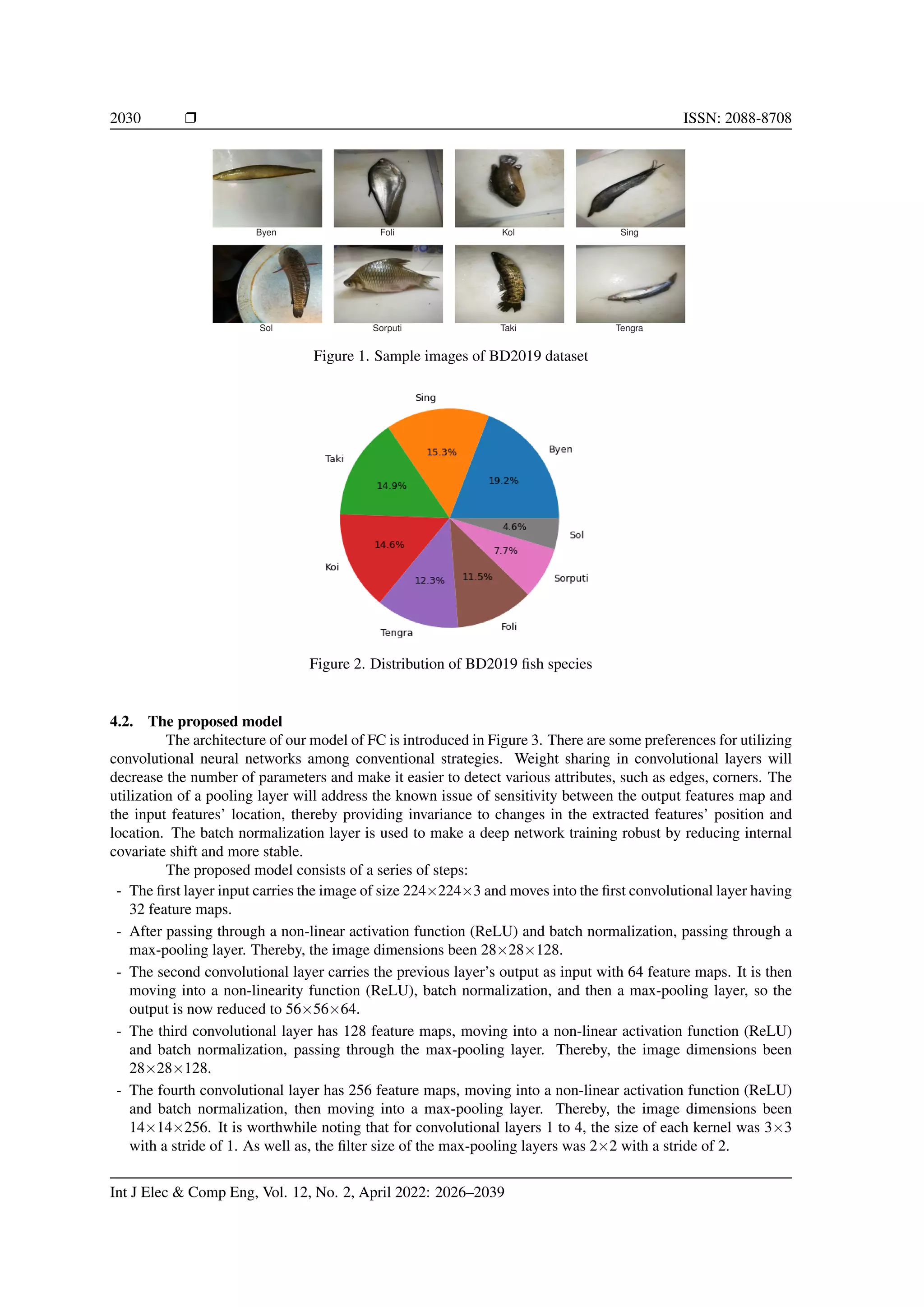
We trained our model on the BDIndigenousFish2019 (BD2019) dataset, which contains eight fish
species from Bangladesh. The BD2019 fish dataset was first time used in [20] for a named approach HLBP.
HLBP is the FC method using hybrid features with SVM classifier. Therefore, it is not fair to compare HLBP
performance with DL-based methods. The BD2019 fish dataset contains 2610 images with eight categories.
Figure 1 illustrates a sample image of each type. The sample species are shown in Figure 2. Images were
resized to 224×224 as per model requirements.

2030 ❒ ISSN: 2088-8708
Figure 1. Sample images of BD2019 dataset
Figure 2. Distribution of BD2019 fish species
4.2. The proposed model
The architecture of our model of FC is introduced in Figure 3. There are some preferences for utilizing
convolutional neural networks among conventional strategies. Weight sharing in convolutional layers will
decrease the number of parameters and make it easier to detect various attributes, such as edges, corners. The
utilization of a pooling layer will address the known issue of sensitivity between the output features map and
the input features’ location, thereby providing invariance to changes in the extracted features’ position and
location. The batch normalization layer is used to make a deep network training robust by reducing internal
covariate shift and more stable.
The proposed model consists of a series of steps:
- The first layer input carries the image of size 224×224×3 and moves into the first convolutional layer having
32 feature maps.
- After passing through a non-linear activation function (ReLU) and batch normalization, passing through a
max-pooling layer. Thereby, the image dimensions been 28×28×128.
- The second convolutional layer carries the previous layer’s output as input with 64 feature maps. It is then
moving into a non-linearity function (ReLU), batch normalization, and then a max-pooling layer, so the
output is now reduced to 56×56×64.
- The third convolutional layer has 128 feature maps, moving into a non-linear activation function (ReLU)
and batch normalization, passing through the max-pooling layer. Thereby, the image dimensions been
28×28×128.
- The fourth convolutional layer has 256 feature maps, moving into a non-linear activation function (ReLU)
and batch normalization, then moving into a max-pooling layer. Thereby, the image dimensions been
14×14×256. It is worthwhile noting that for convolutional layers 1 to 4, the size of each kernel was 3×3
with a stride of 1. As well as, the filter size of the max-pooling layers was 2×2 with a stride of 2.

- The fifth to seventh convolutional layers are connected back-to back. These convolutional layers used 512,
265, 128 feature maps, respectively, followed by non-linearity function (ReLU), batch normalization, and
then max-pooling layer. It is worthwhile noting that for convolutional layers 5 to 7, the size of each kernel
was 5×5 with a stride of 1. As well as, the filter size of the max-pooling layers was 2×2 with a stride of 2.
- The eighth convolutional layer having 64 feature maps, and the size of each kernel is 7×7 with a stride of
1. After moving into a nonlinear activation function (ReLU), the convolutional layer’s output is flattened
through a fully connected layer with 576 feature maps. Then it is connected again to a fully connected layer
with 128 units.
- Then, passing through the Dropout layer with 0.3 is connected again to a fully connected layer with 256
units. The softmax layer is utilized for the output layer with eight units that conform to the number of classes
in the dataset.
Figure 3. The proposed Fish classification schematic, Conv2D: convolution layer, MP: MaxPooling layer,
FC: Fully connected layer
5. EXPERIMENTAL RESULTS AND ANALYSIS
The experiments were conducted in python 3.7 on a computer with Intel Core i7-6700HQ CPU/2.60
GHz/16G/GTX 960. The experiment has been conducted on three Kinds of training splits, 80-20%, 75-25%,

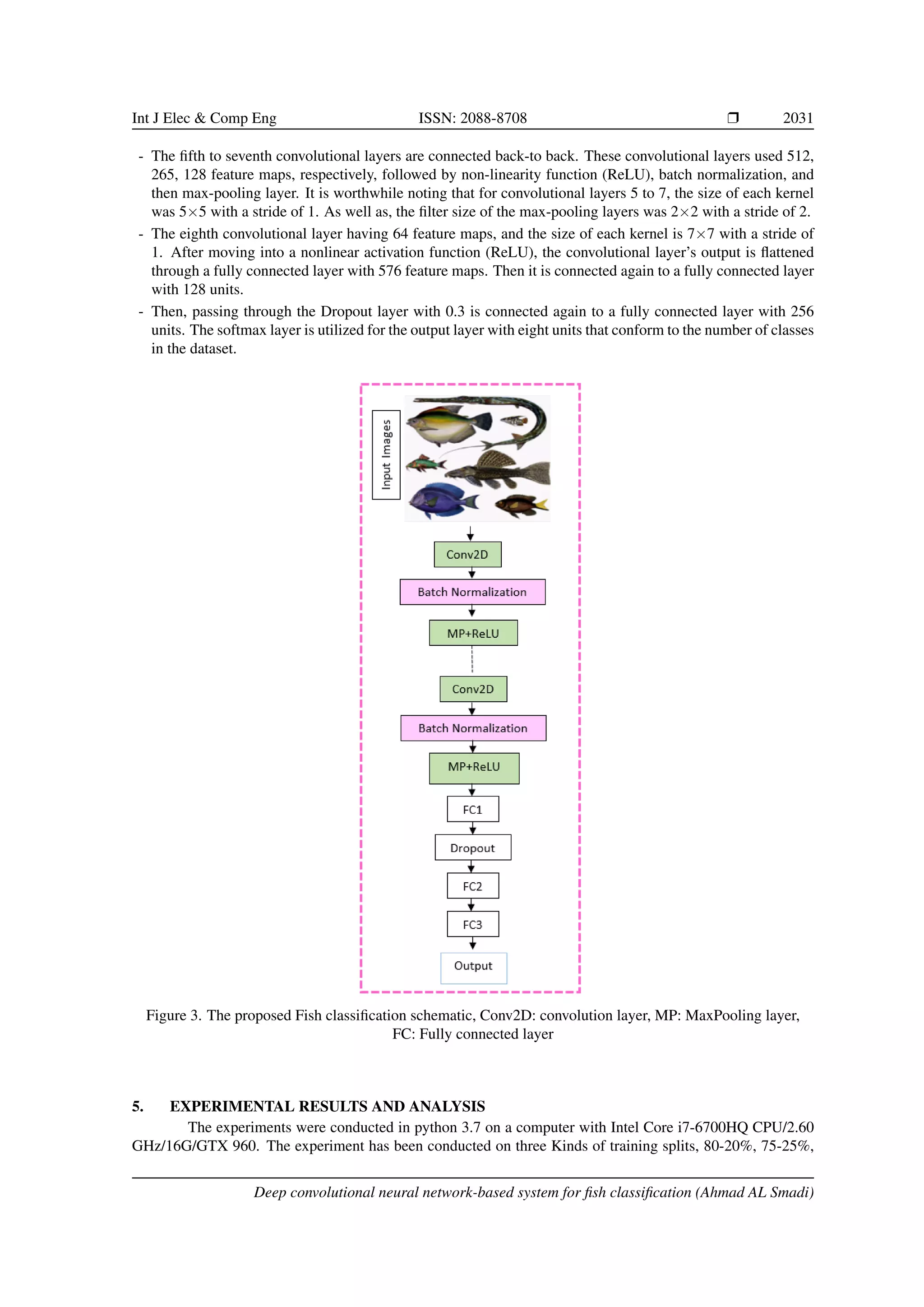
2032 ❒ ISSN: 2088-8708
and 70-30%, with a comparative analysis of different optimization algorithms. Further, we provide an exper-
iment with an augmentation approach. Table 1 illustrates the parameters setting of the proposed model. The
softmax function is used at the last layer; other layers use the Relu activation. Since we used an imbalanced
dataset, the classification accuracy may not be efficient, particularly when we have a multi-class classification
task. Therefore, a confusion matrix for each kind of data splitting is computed that may yield more informa-
tion, i.e., what a classification model gets right and the errors it makes. Thereby, the performance measures
computed from the confusion matrix, including accuracy, sensitivity, and specificity [7].
- Sensitivity is defined as the ability to measure the proportion of positives that are correctly identified. It can
be estimated as (12):
Sensitivity =
TP
TP + FN
(12)
where TP denotes the total number of correctly classified for the actual class, and FN denotes the total
number of not-correctly classified for the actual class.
- Specificity the ability to measure the proportion of negatives that are correctly identified. It can be estimated
as (14):
Specificity =
TN
TN + FP
(13)
where TN denotes the total number of not correctly classified for the actual class and FP denotes the total
number of the correctly classified for the not actual class.
Table 1. Hyper-parameters for the proposed method, used during training and testing,
rectified linear unit (ReLU)
Parameters
Activation function ReLU
Softmax
Learning rate 1e−4
Epochs 50
Steps per epoch 10
Batch size 32
Loss function Categorical cross entropy
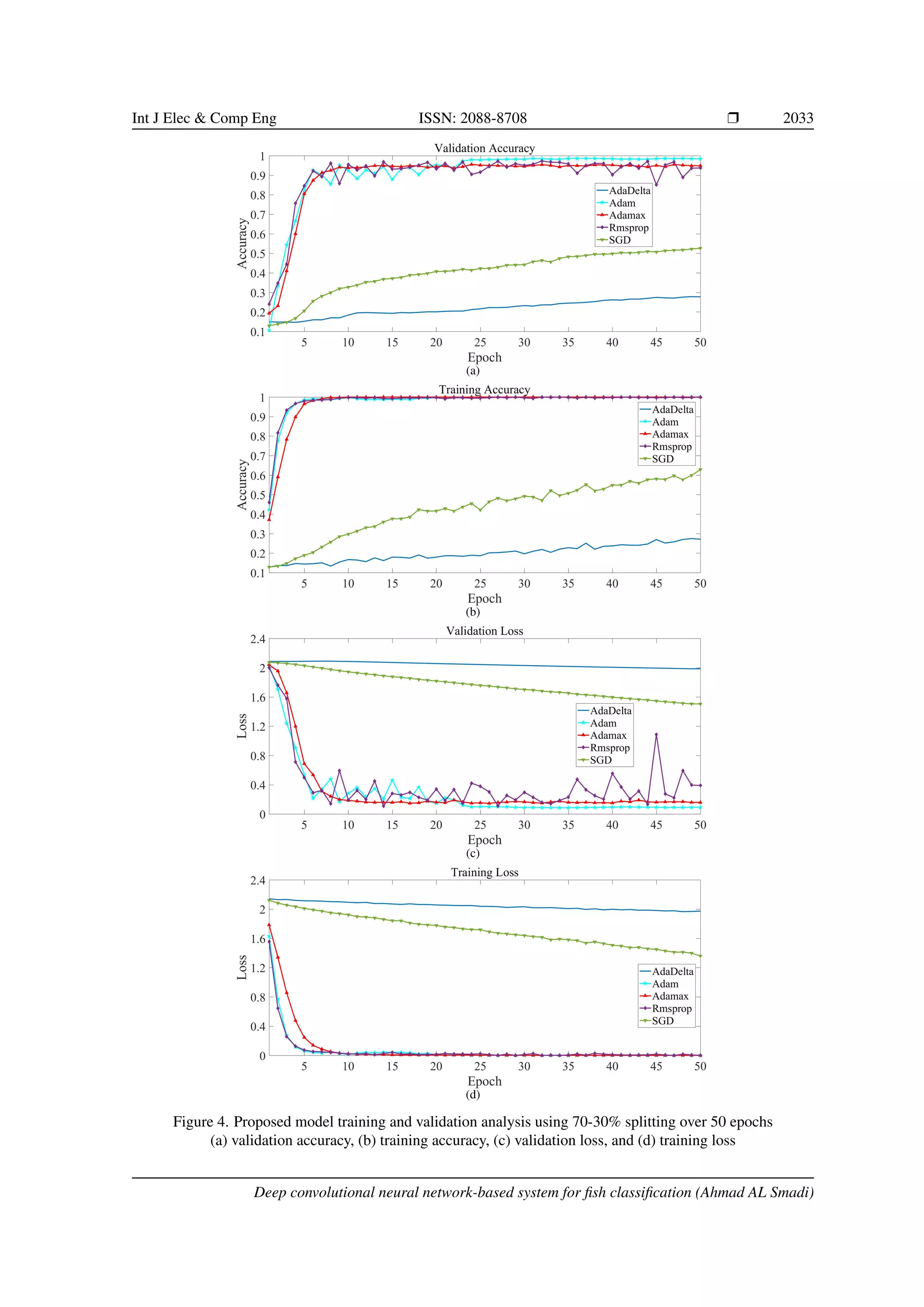
5.1. Experiments on 70-30% data splitting
In this experiment, we divided the dataset for training 70% and testing 30%, which belonged to
eight classes. The testing is used as validation data to validate our model; therefore, the final epoch result
of the validation accuracy is used as test accuracy. Moreover, we performed the analysis on five optimizers.
The average performance results were achieved on 50 epochs. For this experiment, the most successful opti-
mizer is Adam which attained 98.47% testing accuracy. While, Adamax, Rmsprop optimizers were performed
well, and the performances of Adamax, Rmsprop were 94.89%, 93.74%, respectively. Table 2 illustrates the
evaluation metric on testing data for this experiment. The performances of these optimizers are shown in
Figure 4(a) to Figure 4(d). We can observe that the performances of SGD and AdaDelta optimizers were very
bad. The accuracy, sensitivity, and specificity rate on Five optimizers as shown in Table 2. From Table 2, it
can be observed that the Adam optimizer has performed better as compared to other optimizers. Therefore, the
confusion matrix of this experiment is given in Table 3.
Table 2. Evaluation metric on testing data for 70-30% splitting
Optimizers Accuracy % Sensitivity % Specificity %
Adamax 94.89 93.24 95.38
Adam 98.46 97.13 99.04
Rmsprop 93.74 94.21 93.24
AdaDelta 27.71 24.26 28.60
SGD 52.61 49.24 54.26

(a)
(b)
(c)
(d)
Figure 4. Proposed model training and validation analysis using 70-30% splitting over 50 epochs
(a) validation accuracy, (b) training accuracy, (c) validation loss, and (d) training loss

2034 ❒ ISSN: 2088-8708
Table 3. Confusion matrix of the proposed model on the testing dataset concerning 70-30% splitting using
Adam optimizer
Actual Class
Predicted class
Byen Foli Koi Sing Sol Sorputi Taki Tengra
Byen 148 0 1 0 0 1 0 0
Foli 0 88 0 0 1 0 1 0
Koi 1 0 113 0 0 0 0 0
Sing 1 0 0 118 0 1 0 0
Sol 0 1 0 0 34 0 1 0
Sorputi 0 1 1 0 0 58 0 0
Taki 0 1 0 1 0 0 115 0
Tengra 0 0 0 1 0 0 0 95
In this section, the same experiments and analyzes were done, except we divided the dataset for
training 75% and testing 25%. The performance of this experiment through these optimizers is illustrated in
Figure 5 (a) to Figure 5(d) (see in appendix). We can observe that the most successful optimizer is Rm-
sprop which attained 97.24% testing accuracy. While, Adamax and Adam optimizers were performed well,
and Adamax and Adam’s performances were 96.63%, 94.18%, respectively. The performances of SGD and
AdaDelta optimizers were very bad. Table 4 illustrates the evaluation metric on testing data for this experi-
ment. From Table 4, it can be observed that the Rmsprop optimizer has performed better as compared to other
optimizers. Therefore, the confusion matrix of this experiment is given in Table 5.
Table 4. Evaluation metric on testing data for 75-25% splitting. The accuracy, sensitivity, and specificity rate
on five optimizers as shown in Figure 5
Adamax 96.63 95.33 97.17
Adam 94.18 94.34 95.89
Rmsprop 97.24 96.51 98.14
AdaDelta 30.62 27.48 33.06
SGD 49.04 48.52 50.78
Rmsprop optimizer
Actual Class
Predicted Class
Byen 121 0 1 0 0 1 1 1
Foli 0 72 0 0 1 0 1 0
Koi 0 0 92 1 0 1 0 1
Sing 1 0 0 98 0 1 0 0
Sol 0 1 0 0 29 0 0 0
Sorputi 0 0 1 0 0 49 0 0
Taki 0 1 1 1 0 0 94 0
Tengra 1 1 0 0 0 0 0 78
Another experiment has been done in this section in which we divided the dataset for training 80%
and testing 20%. Thereby, the performance of this experiment through these optimizers is illustrated in
Figure 6 (a) to Figure 6(d) (see in appendix). We can observe that the most successful optimizer is Adam
which attained 97.70% testing accuracy. While, Adamax and Rmsprop optimizers were performed well, and
the performances of Adamax and Rmsprop were 95.01%, 93.67%, respectively. The performances of SGD and
AdaDelta optimizers were very bad. Table 6 illustrates the evaluation metric on testing data for this experi-
ment. From Table 6, it can be observed that the Adam optimizer has performed better as compared to other
optimizers. Therefore, the confusion matrix of this experiment is given in Table 7.

Table 6. Evaluation metric on testing data for 80-20% splitting. The accuracy, sensitivity, and specificity rate
on five optimizers as shown in Figure 6
Adamax 95.01 93.78 96.09
Adam 97.70 96.24 98.24
Rmsprop 93.67 92.70 94.24
AdaDelta 28.92 26.89 29.24
SGD 51.91 49.89 52.41
Adam optimizer
Actual class
Predicted Class
Byen 97 1 0 1 0 0 0 1
Foli 1 59 0 0 0 0 0 0
Koi 1 0 74 0 1 0 0 0
Sing 0 0 0 79 0 0 1 0
Sol 0 0 0 0 23 0 0 1
Sorputi 0 0 1 0 0 39 0 0
Taki 0 0 0 0 1 1 76 0
Tengra 0 0 0 0 0 0 1 63
6. DISCUSSION
The strategy of utilizing the CNN to classify fish species requires thousands or indeed tens of thou-
sands of samples to perform duties for training. Therefore, the task of fish species image collection may be a
hard demand to accomplish and to gather adequate information. In this paper, we overcome these issues that
directly involved in decreasing the performance of the fish classification task and introduced the new model
with high accuracy in terms of classification. Among the five optimizers, Adamax was the steadiest one than
AdaDelta, and SGD, which have worse performance. Moreover, the Adam, Adamax, and Rmsprop optimizers
can attain good accuracy at 20 epochs, while the SGD and AdaDelta optimizers could not be attained even
after 50 epochs. From the above discussion, it is uncovered that our proposed CNN architecture with various
optimization algorithms provides promising results for fish classification; thus, the importance of choosing the
hyperparameters of the network. We found that our model performed very well without data augmentation.
Thus, we compared our work with state-of-the-art deep CNNs models, including AlexNet, VGG-16, VGG-19,
Resnet50, adaptive-VGG [25], HDL [26], and DLN-NB [28]. Table 8 (see in appendix) illustrates the com-
parison of results based on deep CNNs models and the developed model. It is worthwhile noting that the deep
CNNs models were trained from scratch, and their results were obtained after 100 iterations.
7. CONCLUSION
This paper introduced a fish classification model with three data splitting and comparative analyses of
five optimizers used in our proposed CNN model. The comparison is made on the publicly available BDIndige-
nousFish2019 dataset. The results showed that three optimizers performed consistently. The Adam optimizer
performed better among these optimizers concerning 70-30% and 80-20% experiments. On the contrary, the
Rmsprop performed better in the 75-25% experiment. Therefore, the findings reinforce the significance of
choosing the hyperparameters of the network used for classification. This paper demonstrated that state-of-the-
art results could be achieved for fish classification through deep CNNs. The experimental result came about
embody that this strategy is productive and dependable among existing deep CNNs models. Further study could
be to examine whether our model can be employed on the other classification tasks. It would be interesting to
investigate if the results can be improved using other artificial intelligence methods such as generative adversar-
ial networks GAN and different transfer learning methods. This makes the research results more reproducible
and comparable.

2036 ❒ ISSN: 2088-8708
APPENDIX
(a)
(b)
(c)
(d)

(a)
(b)
(c)
(d)

2038 ❒ ISSN: 2088-8708
Table 8. Comparison of results based on deep CNNs models and the developed model
Model Number of iterations Accuracy % Sensitivity % Specificity %
AlexNet [39] 100 85.23 84.43 86.21
VGGNet-16 [40] 100 78.56 77.12 79.23
VGGNet-19 [40] 100 76.88 75.51 78.25
ResNet50 [41] 100 87.50 85.12 86.20
Adaptive-VGG [25] 100 91.55 90.37 92.17
HDL [26] 100 90.76 90.53 91.20
DLN-NB [27] 100 94.95 93.17 96.28
Our Method
80-20% 50 97.70 96.24 98.24
75-25% 50 97.24 96.51 98.14
70-30% 50 98.46 97.13 99.04
REFERENCES
[1] P. Goswami, A. Mukherjee, M. Maiti, S. K. S. Tyagi, and L. Yang, “A neural network based optimal re-
source allocation method for secure IIoT network,” IEEE Internet of Things Journal, pp. 1–1, 2021, doi:
10.1109/jiot.2021.3084636.
[2] A. M. Al-Smadi, A. Al-Smadi, R. M. A. Aloglah, N. Abu-darwish, and A. Abugabah, “Files cryptography based on
one-time pad algorithm,” International Journal of Electrical and Computer Engineering (IJECE), vol. 11, no. 3, pp.
2335-2342, Jun. 2021, doi: 10.11591/ijece.v11i3.pp2335-2342.
[3] A. A. Alsanabani, M. A. Ahmed, and A. M. A. Smadi, “Vehicle counting using detecting-tracking combinations: A
comparative analysis,” in 2020 The 4th International Conference on Video and Image Processing. ACM, Dec 2020,
doi: 10.1145/3447450.3447458.
[4] A. A. Smadi, S. Yang, A. Mehmood, A. Abugabah, M. Wang, and M. Bashir, “Smart pansharpening approach
using kernel-based image filtering,” IET Image Processing, vol. 15, no. 11, pp. 2629-2642, May 2021, doi:
10.1049/ipr2.12251.
[5] V. Allken, N. O. Handegard, S. Rosen, T. Schreyeck, T. Mahiout, and K. Malde, “Fish species identification using a
convolutional neural network trained on synthetic data,” ICES Journal of Marine Science, vol. 76, no. 1, pp. 342–349,
Oct. 2018, doi: 10.1093/icesjms/fsy147.
[6] M. A. Iqbal, Z. Wang, Z. A. Ali, and S. Riaz, “Automatic fish species classification using deep convolutional neural
networks,” Wireless Personal Communications, vol. 116, no. 2, pp. 1043–1053, Aug. 2019, doi: 10.1007/s11277-
019-06634-1.
[7] F. J. P. Montalbo and A. A. Hernandez, “Classification of fish species with augmented data using deep convolutional
neural network,” in 2019 IEEE 9th International Conference on System Engineering and Technology (ICSET), Oct.
2019, doi: 10.1109/icsengt.2019.8906433.
[8] N. E. M. Khalifa, M. H. N. Taha, and A. E. Hassanien, “Aquarium family fish species identification system using
deep neural networks,” in Advances in Intelligent Systems and Computing, vol. 845, Aug 2018, pp. 347-356, doi:
10.1007/978-3-319-99010-1 32.
[9] M. K. Alsmadi and I. Almarashdeh, “A survey on fish classification techniques,” Journal of King Saud University -
Computer and Information Sciences, Jul 2020, doi: 10.1016/j.jksuci.2020.07.005.
[10] K. Hüssy, H. Mosegaard, C. M. Albertsen, E. E. Nielsen, J. Hemmer-Hansen, and M. Eero, “Evaluation of otolith
shape as a tool for stock discrimination in marine fishes using baltic sea cod as a case study,” Fisheries Research, vol.
174, pp. 210-218, Feb 2016, doi: 10.1016/j.fishres.2015.10.010.
[11] M. K. Alsmadi, M. Tayfour, R. A. Alkhasawneh, U. Badawi, I. Almarashdeh, and F. Haddad, “Robust features
extraction for general fish classification,” International Journal of Electrical and Computer Engineering (IJECE),
vol. 9, no. 6, pp. 5192-5204, Dec 2019, doi: 10.11591/ijece.v9i6.pp5192-5204.
[12] Y. Ma, P. Zhang, and Y. Tang, “Research on fish image classification based on transfer learning and convolutional neu-
ral network model,” in 2018 14th International Conference on Natural Computation, Fuzzy Systems and Knowledge
Discovery (ICNC-FSKD), Jul. 2018, doi: 10.1109/fskd.2018.8686892.
[13] M. Alsmadi, K. Omar, S. Noah, and I. Almarashde, “A hybrid memetic algorithm with back-propagation classifier for
fish classification based on robust features extraction from PLGF and shape measurements,” Information Technology
Journal, vol. 10, no. 5, pp. 944-954, Apr. 2011, doi: 10.3923/itj.2011.944.954.
[14] G. French, et al., “Deep neural networks for analysis of fisheries surveillance video and automated monitoring of fish
discards,” ICES Journal of Marine Science, vol. 77, no. 4, pp. 1340–1353, Aug 2019, doi: 10.1093/icesjms/fsz149.
[15] B. Iscimen, Y. Kutlu, A. Uyan, and C. Turan, “Classification of fish species with two dorsal fins using centroid-
contour distance,” in 2015 23nd Signal Processing and Communications Applications Conference (SIU), May 2015,
doi: 10.1109/siu.2015.7130252.
[16] S. A. Siddiqui, et al., “Automatic fish species classification in underwater videos: exploiting pre-trained deep neural
network models to compensate for limited labelled data,” ICES Journal of Marine Science, vol. 75, no. 1, pp. 374–

389, Jul. 2017, doi: 10.1093/icesjms/fsx109.
[17] Y.-H. Hsiao, C.-C. Chen, S.-I. Lin, and F.-P. Lin, “Real-world underwater fish recognition and identification, using
sparse representation,” Ecological Informatics, vol. 23, pp. 13–21, Sep. 2014, doi: 10.1016/j.ecoinf.2013.10.002.
[18] I. Sharmin, N. F. Islam, I. Jahan, T. A. Joye, M. R. Rahman, and M. T. Habib, “Machine vision based local fish
recognition,” SN Applied Sciences, vol. 1, no. 12, Nov. 2019, doi: 10.1007/s42452-019-1568-z.
[19] M. K. Alsmadi, “Hybrid genetic algorithm with tabu search with back-propagation algorithm for fish classification:
Determining the appropriate feature set,” International Journal of Applied Engineering Research, vol. 14, no. 23, pp.
4387-4396, 2019.
[20] M. A. Islam, M. R. Howlader, U. Habiba, R. H. Faisal, and M. M. Rahman, “Indigenous fish clas-
sification of bangladesh using hybrid features with SVM classifier,” in 2019 International Conference on
Computer, Communication, Chemical, Materials and Electronic Engineering (IC4ME2), Jul. 2019, doi:
10.1109/ic4me247184.2019.9036679.
[21] D. Rathi, S. Jain, and S. Indu, “Underwater fish species classification using convolutional neural network and deep
learning,” in 2017 Ninth International Conference on Advances in Pattern Recognition (ICAPR), Dec. 2017, doi:
10.1109/icapr.2017.8593044.
[22] Z. Zheng, et al., “Fish recognition from a vessel camera using deep convolutional neural network and data
augmentation,” in 2018 OCEANS - MTS/IEEE Kobe Techno-Oceans (OTO), May 2018, doi: 10.1109/ocean-
skobe.2018.8559314.
[23] T. Miyazono and T. Saitoh, “Fish species recognition based on CNN using annotated image,” in IT Convergence and
Security 2017, Aug. 2017, pp. 156-163, doi: 10.1007/978-981-10-6451-7 19.
[24] S. Cui, Y. Zhou, Y. Wang, and L. Zhai, “Fish detection using deep learning,” Applied Computational Intelligence and
Soft Computing, vol. 2020, pp. 1-13, Jan. 2020, doi: 10.1155/2020/3738108.
[25] F. Kratzert and H. Mader, “Fish species classification in underwater video monitoring using convolutional neural
networks,” May 2018, doi: 10.31223/osf.io/dxwtz.
[26] H. S. Chhabra, A. K. Srivastava, and R. Nijhawan, “A hybrid deep learning approach for automatic fish classifi-
cation,” in Proceedings of ICETIT 2019, Springer International Publishing, Sep. 2019, vol. 605, pp. 427-436, doi:
10.1007/978-3-030-30577-2 37.
[27] N. S. Abinaya, D. Susan, and R. Kumar, “Naive bayesian fusion based deep learning networks for multiseg-
mented classification of fishes in aquaculture industries,” Ecological Informatics, vol. 61, p. 101248, Mar. 2021,
doi: 10.1016/j.ecoinf.2021.101248.
[28] D. T. Mane and U. V. Kulkarni, “A survey on supervised convolutional neural network and its major applications,” in
Deep Learning and Neural Networks, IGI Global, 2020, pp. 1058-1071, doi: 10.4018/978-1-7998-0414-7.ch059.
[29] I. Goodfellow, Y. Bengio, A. Courville, and Y. Bengio, Deep learning, MIT press Cambridge, 2016, vol. 1, no. 2.
[30] L. Bottou, “Large-scale machine learning with stochastic gradient descent,” in Proceedings of COMPSTAT'2010,
Physica-Verlag HD, 2010, pp. 177-186, doi: 10.1007/978-3-7908-2604-3 16.
[31] M. D. Zeiler, “ADADELTA: an adaptive learning rate method,” CoRR, vol. abs/1212.5701, 2012.
[32] J. Duchi, E. Hazan, and Y. Singer, “Adaptive subgradient methods for online learning and stochastic optimization,” J.
Mach. Learn. Res., vol. 12, pp. 2121–2159, Jul. 2011, doi: 10.5555/1953048.2021068.
[33] G. Hinton, N. Srivastava, and K. Swersky, “Neural networks for machine learning lecture 6a overview of mini-batch
gradient descent,” Cited on, vol. 14, no. 8, p. 2, 2012.
[34] D. P. Kingma and J. Ba, “Adam: A method for stochastic optimization,” arXiv preprint arXiv:1412.6980, 2014.
[35] E. M. Dogo, O. J. Afolabi, N. I. Nwulu, B. Twala, and C. O. Aigbavboa, “A comparative analysis of gradient descent-
based optimization algorithms on convolutional neural networks,” in 2018 International Conference on Computa-
tional Techniques, Electronics and Mechanical Systems (CTEMS), Dec. 2018, doi: 10.1109/ctems.2018.8769211.
[36] A. Mehmood, et al., “A transfer learning approach for early diagnosis of alzheimer’s disease on MRI images,” Neu-
roscience, vol. 460, pp. 43–52, Apr. 2021, doi: 10.1016/j.neuroscience.2021.01.002.
[37] R. C. Gonzalez, “Deep convolutional neural networks [lecture notes],” IEEE Signal Processing Magazine, vol. 35,
no. 6, pp. 79–87, Nov. 2018, doi: 10.1109/msp.2018.2842646.
[38] G. J. Scott, M. R. England, W. A. Starms, R. A. Marcum, and C. H. Davis, “Training deep convolutional neural
networks for land–cover classification of high-resolution imagery,” IEEE Geoscience and Remote Sensing Letters,
vol. 14, no. 4, pp. 549–553, Apr 2017, doi: 10.1109/lgrs.2017.2657778.
[39] A. Krizhevsky, I. Sutskever, and G. E. Hinton, “ImageNet classification with deep convolutional neural networks,”
Communications of the ACM, vol. 60, no. 6, pp. 84–90, May 2017, doi: 10.1145/3065386.
[40] K. Simonyan and A. Zisserman, “Very deep convolutional networks for large-scale image recognition,” arXiv preprint
arXiv:1409.1556, 2014.
[41] K. He, X. Zhang, S. Ren, and J. Sun, “Deep residual learning for image recognition,” in Proceedings of the IEEE
conference on computer vision and pattern recognition, 2016, pp. 770-778, doi: 10.1109/CVPR.2016.90.

Deep convolutional neural network-based system for fish classification

More Related Content

Similar to Deep convolutional neural network-based system for fish classification

More from IJECEIAES

Recently uploaded

Deep convolutional neural network-based system for fish classification