The document discusses traditional methods for sizing valves for liquid flow. It explains that improper valve sizing can be expensive and cause process issues. The traditional method involves determining the valve sizing coefficient (Cv) based on published values, accounting for factors like pressure differential, fluid properties, and viscosity. A key equation relates Cv to flow rate, with corrections for non-ideal fluids. Graphs are provided to correct for viscosity and determine the actual required Cv for a given application. Selecting a valve with a Cv equal or higher than required will ensure sufficient flow.

1. Valve Sizing Calculations (Traditional Method)
626
Technical
Introduction
Fisher®
regulators and valves have traditionally been sized using
equations derived by the company. There are now standardized
calculations that are becoming accepted worldwide. Some product
literature continues to demonstrate the traditional method, but
the trend is to adopt the standardized method. Therefore, both
methods are covered in this application guide.
Improper valve sizing can be both expensive and inconvenient.
A valve that is too small will not pass the required flow, and
the process will be starved. An oversized valve will be more
expensive, and it may lead to instability and other problems.
The days of selecting a valve based upon the size of the pipeline
are gone. Selecting the correct valve size for a given application
requires a knowledge of process conditions that the valve will
actually see in service. The technique for using this information
to size the valve is based upon a combination of theory
and experimentation.
Sizing for Liquid Service
Using the principle of conservation of energy, Daniel Bernoulli
found that as a liquid flows through an orifice, the square of the
fluid velocity is directly proportional to the pressure differential
across the orifice and inversely proportional to the specific gravity
of the fluid. The greater the pressure differential, the higher the
velocity; the greater the density, the lower the velocity. The
volume flow rate for liquids can be calculated by multiplying the
fluid velocity times the flow area.
By taking into account units of measurement, the proportionality
relationship previously mentioned, energy losses due to friction
and turbulence, and varying discharge coefficients for various
types of orifices (or valve bodies), a basic liquid sizing equation
can be written as follows
Q = CV
∆P / G (1)
where:
Q = Capacity in gallons per minute
Cv
= Valve sizing coefficient determined experimentally for
each style and size of valve, using water at standard
conditions as the test fluid
∆P = Pressure differential in psi
G = Specific gravity of fluid (water at 60°F = 1.0000)
Thus, Cv
is numerically equal to the number of U.S. gallons of
water at 60°F that will flow through the valve in one minute when
the pressure differential across the valve is one pound per square
inch. Cv
varies with both size and style of valve, but provides an
index for comparing liquid capacities of different valves under a
standard set of conditions.
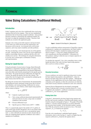
To aid in establishing uniform measurement of liquid flow capacity
coefficients (Cv
) among valve manufacturers, the Fluid Controls
Institute (FCI) developed a standard test piping arrangement,
shown in Figure 1. Using such a piping arrangement, most
valve manufacturers develop and publish Cv
information for
their products, making it relatively easy to compare capacities of
competitive products.
To calculate the expected Cv
for a valve controlling water or other
liquids that behave like water, the basic liquid sizing equation
above can be re-written as follows
CV
= Q
G
∆P
(2)
Viscosity Corrections
Viscous conditions can result in significant sizing errors in using
the basic liquid sizing equation, since published Cv
values are
based on test data using water as the flow medium. Although the
majority of valve applications will involve fluids where viscosity
corrections can be ignored, or where the corrections are relatively
small, fluid viscosity should be considered in each valve selection.
Emerson Process Management has developed a nomograph
(Figure 2) that provides a viscosity correction factor (Fv
). It can
be applied to the standard Cv
coefficient to determine a corrected
coefficient (Cvr
) for viscous applications.
Finding Valve Size
Using the Cv
determined by the basic liquid sizing equation and
the flow and viscosity conditions, a fluid Reynolds number can be
found by using the nomograph in Figure 2. The graph of Reynolds
number vs. viscosity correction factor (Fv
) is used to determine
the correction factor needed. (If the Reynolds number is greater
than 3500, the correction will be ten percent or less.) The actual
required Cv
(Cvr
) is found by the equation:
Cvr
= FV
CV
(3)
From the valve manufacturer’s published liquid capacity
information, select a valve having a Cv
equal to or higher than the
required coefficient (Cvr
) found by the equation above.
Figure 1. Standard FCI Test Piping for Cv
Measurement
PRESSURE
INDICATORS
∆P ORIFICE
METER
INLET VALVE TEST VALVE LOAD VALVE
FLOW

2. 627
Technical
Valve Sizing Calculations (Traditional Method)
3000
3,000
4,000
6,000
8,000
10,000
20,000
30,000
40,000
60,000
80,000
100,000
200,000
300,000
400,000
600,000
800,000
1,000,000
1 2 3 4
C
INDEX 1 2 3 4
2000
2,000
1,000
2,000
2,000
3,000
3,000
4,000
4,000
6,000
6,000
8,000
8,000
10,000
10,000
800
600
400
300
200
100
80
60
40
30
20
10
8
6
4
3
2
1
1,000
1,000
2,000
2,000
3,000
3,000
4,000
4,000
6,000
6,000
8,000
8,000
10,000
10,000
20,000
20,000
30,000
30,000
40,000
40,000
60,000
60,000
80,000
80,000
100,000
100,000
200,000
300,000
400,000
800
800
600
600
400
400
300
300
200
200
100
100
80
80
60
60
40
40
35
32.6
30
20
10
8
6
4
3
2
1
0.8
0.6
0.4
0.3
0.2
0.1
0.08
0.06
0.04
0.03
0.02
0.01
1,000
1,000
800
600
800
600
400
300
200
100
80
60
40
30
20
400
300
200
100
80
60
40
30
20
10
10
8
8
6
6
4
4
3
3
2
2
1
0.8
0.6
0.4
0.2
0.1
0.3
1
0.8
0.6
0.4
0.3
0.2
0.1
0.08
0.06
0.04
0.04
0.06
0.08
0.03
0.03
0.02
0.02
0.01
0.01
0.008
0.008
0.006
0.006
0.004
0.004
0.003
0.003
0.002
0.002
0 .001
0.001
0.0008
0.0008
0.0006
0.0006
0.0004
0.0004
0.0003
0.0003
0.0002
0.0002
0.0001
0.0001
1000
800
600
400
300
200
100
80
60
40
30
20
10
8
6
4
3
2
1
0.8
0.6
0.4
0.3
0.2
0.1
0.08
0.06
0.04
0.03
0.02
0.01
Figure 2. Nomograph for Determining Viscosity Correction
Nomograph Instructions
Use this nomograph to correct for the effects of viscosity. When
assembling data, all units must correspond to those shown on the
nomograph. For high-recovery, ball-type valves, use the liquid
flow rate Q scale designated for single-ported valves. For butterfly
and eccentric disk rotary valves, use the liquid flow rate Q scale
designated for double-ported valves.
Nomograph Equations
1. Single-Ported Valves: NR
= 17250
Q
CV
νCS
2. Double-Ported Valves: NR
= 12200
Q
CV
νCS
Nomograph Procedure
1. Lay a straight edge on the liquid sizing coefficient on Cv
scale and flow rate on Q scale. Mark intersection on index
line. Procedure A uses value of Cvc
; Procedures B and C use
value of Cvr
.
2. Pivot the straight edge from this point of intersection with
index line to liquid viscosity on proper n scale. Read Reynolds
number on NR
scale.
3. Proceed horizontally from intersection on NR
scale to proper
curve, and then vertically upward or downward to Fv
scale.
Read Cv
correction factor on Fv
scale.
3,000
4,000
6,000
8,000
10,000
20,000
30,000
40,000
60,000
80,000
100,000
200,000
300,000
400,000
600,000
800,000
1,000,000
1 2 3 4 6
INDEX
8 10 20 30 40 60 80 100 200
1 2 3 4 6 8 10 20 30 40 60 80 100 200
2,000
1,000
2,000
2,000
3,000
3,000
4,000
4,000
6,000
6,000
8,000
8,000
10,000
10,000
800
600
400
300
200
100
80
60
40
30
20
10
8
6
4
3
2
1
1,000
1,000
2,000
2,000
3,000
3,000
4,000
4,000
6,000
6,000
8,000
8,000
10,000
10,000
20,000
20,000
30,000
30,000
40,000
40,000
60,000
60,000
80,000
80,000
100,000
100,000
200,000
300,000
400,000
800
800
600
600
400
400
300
300
200
200
100
100
80
80
60
60
40
40
35
32.6
30
20
10
8
6
4
3
2
1
0.8
0.6
0.4
0.3
0.2
0.1
0.08
0.06
0.04
0.03
0.02
0.01
1,000
800
600
400
300
200
100
80
60
40
30
20
10
8
6
4
3
2
1
0.8
0.6
0.4
0.2
0.1
0.3
0.04
0.06
0.08
0.03
0.02
0.01
0.008
0.008
0.006
0.006
0.004
0.004
0.003
0.003
0.002
0.002
0 .001
0.001
0.0008
0.0008
0.0006
0.0006
0.0004
0.0004
0.0003
0.0003
0.0002
0.0002
0.0001
0.0001
1000
800
600
400
300
200
100
80
60
40
30
20
10
8
6
4
3
2
1
0.8
0.6
0.4
0.3
0.2
0.1
0.08
0.06
0.04
0.03
0.02
0.01
LIQUID
FLOW
COEFFICIENT,
C
V
CV
LIQUID
FLOW
RATE
(SINGLE
PORTED
ONLY),
GPM
Q
LIQUID
FLOW
RATE
(DOUBLE
PORTED
ONLY),
GPM
KINEMATIC
VISCOSITY
V
CS
-
CENTISTOKES
VISCOSITY
-
SAYBOLT
SECONDS
UNIVERSAL
REYNOLDS
NUMBER
-
N
R
CV
CORRECTION FACTOR, FV
INDEX
CV
CORRECTION FACTOR, FV
HR
FV
FOR PREDICTING PRESSURE DROP
FOR SELECTING VALVE SIZE
FOR PREDICTING
FLOW RATE
3,000
4,000
6,000
8,000
10,000
20,000
30,000
40,000
60,000
80,000
100,000
200,000
300,000
400,000
600,000
800,000
1,000,000
1 2 3 4 6
C
INDEX
8 10 20 30 40 60
1 2 3 4 6 8 10 20 30 40 60
2,000
1,000
2,000
2,000
3,000
3,000
4,000
4,000
6,000
6,000
8,000
8,000
10,000
10,000
800
600
400
300
200
100
80
60
40
30
20
10
8
6
4
3
2
1
1,000
1,000
2,000
2,000
3,000
3,000
4,000
4,000
6,000
6,000
8,000
8,000
10,000
10,000
20,000
20,000
30,000
30,000
40,000
40,000
60,000
60,000
80,000
80,000
100,000
100,000
200,000
300,000
400,000
800
800
600
600
400
400
300
300
200
200
100
100
80
80
60
60
40
40
35
32.6
30
20
10
8
6
4
3
2
1
0.8
0.6
0.4
0.3
0.2
0.1
0.08
0.06
0.04
0.03
0.02
0.01
1,000
800
600
400
300
200
100
80
60
40
30
20
10
8
6
4
3
2
1
0.8
0.6
0.4
0.2
0.1
0.3
0.04
0.06
0.08
0.03
0.02
0.01
0.008
0.008
0.006
0.006
0.004
0.004
0.003
0.003
0.002
0.002
0 .001
0.001
0.0008
0.0008
0.0006
0.0006
0.0004
0.0004
0.0003
0.0003
0.0002
0.0002
0.0001
0.0001
1000
800
600
400
300
200
100
80
60
40
30
20
10
8
6
4
3
2
1
0.8
0.6
0.4
0.3
0.2
0.1
0.08
0.06
0.04
0.03
0.02
0.01

3. Valve Sizing Calculations (Traditional Method)
628
Technical
Predicting Flow Rate
Select the required liquid sizing coefficient (Cvr
) from the
manufacturer’s published liquid sizing coefficients (Cv
) for the
style and size valve being considered. Calculate the maximum
flow rate (Qmax
) in gallons per minute (assuming no viscosity
correction required) using the following adaptation of the basic
liquid sizing equation:
Qmax
= Cvr
ΔP / G (4)
Then incorporate viscosity correction by determining the fluid
Reynolds number and correction factor Fv
from the viscosity
correction nomograph and the procedure included on it.
Calculate the predicted flow rate (Qpred
) using the formula:
Qpred
=
Qmax
FV
(5)
Predicting Pressure Drop
Select the required liquid sizing coefficient (Cvr
) from the published
liquid sizing coefficients (Cv
) for the valve style and size being
considered. Determine the Reynolds number and correct factor Fv
from the nomograph and the procedure on it. Calculate the sizing
coefficient (Cvc
) using the formula:
CVC
=
Cvr
Fv
(6)
Calculate the predicted pressure drop (∆Ppred
) using the formula:
ΔPpred
= G (Q/Cvc
)2
(7)
Flashing and Cavitation
The occurrence of flashing or cavitation within a valve can have a
significant effect on the valve sizing procedure. These two related
physical phenomena can limit flow through the valve in many
applications and must be taken into account in order to accurately
size a valve. Structural damage to the valve and adjacent piping
may also result. Knowledge of what is actually happening within
the valve might permit selection of a size or style of valve which
can reduce, or compensate for, the undesirable effects of flashing
or cavitation.
The “physical phenomena” label is used to describe flashing and
cavitation because these conditions represent actual changes in
the form of the fluid media. The change is from the liquid state
to the vapor state and results from the increase in fluid velocity at
or just downstream of the greatest flow restriction, normally the
valve port. As liquid flow passes through the restriction, there is a
necking down, or contraction, of the flow stream. The minimum
cross-sectional area of the flow stream occurs just downstream of
the actual physical restriction at a point called the vena contracta,
as shown in Figure 3.
To maintain a steady flow of liquid through the valve, the velocity
must be greatest at the vena contracta, where cross sectional
area is the least. The increase in velocity (or kinetic energy) is
accompanied by a substantial decrease in pressure (or potential
energy) at the vena contracta. Farther downstream, as the fluid
stream expands into a larger area, velocity decreases and pressure
increases. But, of course, downstream pressure never recovers
completely to equal the pressure that existed upstream of the
valve. The pressure differential (∆P) that exists across the valve
Figure 3. Vena Contracta
Figure 4. Comparison of Pressure Profiles for
High and Low Recovery Valves
VENA CONTRACTA
RESTRICTION
FLOW
FLOW
P1
P2
P1
P2
P2
P2
HIGH RECOVERY
LOW RECOVERY
P1

4. 629
Technical
Valve Sizing Calculations (Traditional Method)
is a measure of the amount of energy that was dissipated in the
valve. Figure 4 provides a pressure profile explaining the differing
performance of a streamlined high recovery valve, such as a ball
valve and a valve with lower recovery capabilities due to greater
internal turbulence and dissipation of energy.
Regardless of the recovery characteristics of the valve, the pressure
differential of interest pertaining to flashing and cavitation is the
differential between the valve inlet and the vena contracta. If
pressure at the vena contracta should drop below the vapor pressure
of the fluid (due to increased fluid velocity at this point) bubbles
will form in the flow stream. Formation of bubbles will increase
greatly as vena contracta pressure drops further below the vapor
pressure of the liquid. At this stage, there is no difference between
flashing and cavitation, but the potential for structural damage to
the valve definitely exists.
If pressure at the valve outlet remains below the vapor pressure
of the liquid, the bubbles will remain in the downstream system
and the process is said to have “flashed.” Flashing can produce
serious erosion damage to the valve trim parts and is characterized
by a smooth, polished appearance of the eroded surface. Flashing
damage is normally greatest at the point of highest velocity, which
is usually at or near the seat line of the valve plug and seat ring.
However, if downstream pressure recovery is sufficient to raise the
outlet pressure above the vapor pressure of the liquid, the bubbles
will collapse, or implode, producing cavitation. Collapsing of the
vapor bubbles releases energy and produces a noise similar to what
one would expect if gravel were flowing through the valve. If the
bubbles collapse in close proximity to solid surfaces, the energy
released gradually wears the material leaving a rough, cylinder
like surface. Cavitation damage might extend to the downstream
pipeline, if that is where pressure recovery occurs and the bubbles
collapse. Obviously, “high recovery” valves tend to be more
subject to cavitation, since the downstream pressure is more likely
to rise above the vapor pressure of the liquid.
Choked Flow
Aside from the possibility of physical equipment damage due to
flashing or cavitation, formation of vapor bubbles in the liquid flow
stream causes a crowding condition at the vena contracta which
tends to limit flow through the valve. So, while the basic liquid
sizing equation implies that there is no limit to the amount of flow
through a valve as long as the differential pressure across the valve
increases, the realities of flashing and cavitation prove otherwise.
If valve pressure drop is increased slightly beyond the point where
bubbles begin to form, a choked flow condition is reached. With
constant upstream pressure, further increases in pressure drop (by
reducing downstream pressure) will not produce increased flow.
The limiting pressure differential is designated ∆Pallow
and the valve
recovery coefficient (Km
) is experimentally determined for each
valve, in order to relate choked flow for that particular valve to the
basic liquid sizing equation. Km
is normally published with other
valve capacity coefficients. Figures 5 and 6 show these flow vs.
pressure drop relationships.
Figure 5. Flow Curve Showing Cv
and Km
CHOKED FLOW
PLOT OF EQUATION (1)
P1
= CONSTANT
∆P (ALLOWABLE)
Cv
Q(gpm) Km
ΔP
Figure 6. Relationship Between Actual ∆P and ∆P Allowable
∆P (ALLOWABLE)
ACTUAL ∆P
PREDICTED FLOW USING
ACTUAL ∆P
Cv
Q(gpm)
ACTUAL
FLOW
ΔP

5. Valve Sizing Calculations (Traditional Method)
630
Technical
Use the following equation to determine maximum allowable
pressure drop that is effective in producing flow. Keep in mind,
however, that the limitation on the sizing pressure drop, ∆Pallow
,
does not imply a maximum pressure drop that may be controlled y
the valve.
∆Pallow
= Km
(P1
- rc
P v
) (8)
where:
∆Pallow
= maximum allowable differential pressure for sizing
purposes, psi
Km
= valve recovery coefficient from manufacturer’s literature
P1
= body inlet pressure, psia
rc
= critical pressure ratio determined from Figures 7 and 8
Pv
= vapor pressure of the liquid at body inlet temperature,
psia (vapor pressures and critical pressures for
many common liquids are provided in the Physical
Constants of Hydrocarbons and Physical Constants
of Fluids tables; refer to the Table of Contents for the
page number).
After calculating ∆Pallow
, substitute it into the basic liquid sizing
equation Q = CV
∆P / G to determine either Q or Cv
. If the
actual ∆P is less the ∆Pallow
, then the actual ∆P should be used in
the equation.
The equation used to determine ∆Pallow
should also be used to
calculate the valve body differential pressure at which significant
cavitation can occur. Minor cavitation will occur at a slightly lower
pressure differential than that predicted by the equation, but should
produce negligible damage in most globe-style control valves.
Consequently, initial cavitation and choked flow occur nearly
simultaneously in globe-style or low-recovery valves.
However, in high-recovery valves such as ball or butterfly valves,
significant cavitation can occur at pressure drops below that which
produces choked flow. So although ∆Pallow
and Km
are useful in
predicting choked flow capacity, a separate cavitation index (Kc
) is
needed to determine the pressure drop at which cavitation damage
will begin (∆Pc
) in high-recovery valves.
The equation can e expressed:
∆PC
= KC
(P1
- PV
) (9)
This equation can be used anytime outlet pressure is greater than
the vapor pressure of the liquid.
Addition of anti-cavitation trim tends to increase the value of Km
.
In other words, choked flow and incipient cavitation will occur at
substantially higher pressure drops than was the case without the
anti-cavitation accessory.
Figure 7. Critical Pressure Ratios for Water Figure 8. Critical Pressure Ratios for Liquid Other than Water
Use this curve for water. Enter on the abscissa at the water vapor pressure at the
valve inlet. Proceed vertically to intersect the
curve. Move horizontally to the left to read the critical
pressure ratio, rc
, on the ordinate.
Use this curve for liquids other than water. Determine the vapor
pressure/critical pressure ratio by dividing the liquid vapor pressure
at the valve inlet by the critical pressure of the liquid. Enter on the abscissa at the
ratio just calculated and proceed vertically to
intersect the curve. Move horizontally to the left and read the critical
pressure ratio, rc
, on the ordinate.
1.0
0.9
0.8
0.7
0.6
0.5
CRITICAL
PRESSURE
RATIO—r
c
0 0.20 0.40 0.60 0.80 1.0
VAPOR PRESSURE, PSIA
CRITICAL PRESSURE, PSIA
1.0
0.9
0.8
0.7
0.6
0.5
CRITICAL
PRESSURE
RATIO—r
c
0 500 1000 1500 2000 2500 3000 3500
VAPOR PRESSURE, PSIA

6. 631
Technical
Valve Sizing Calculations (Traditional Method)
Liquid Sizing Summary
The most common use of the basic liquid sizing equation is
to determine the proper valve size for a given set of service
conditions. The first step is to calculate the required Cv
by using
the sizing equation. The ∆P used in the equation must be the actual
valve pressure drop or ∆Pallow
, whichever is smaller. The second
step is to select a valve, from the manufacturer’s literature, with a
Cv
equal to or greater than the calculated value.
Accurate valve sizing for liquids requires use of the dual
coefficients of Cv
and Km
. A single coefficient is not sufficient
to describe both the capacity and the recovery characteristics of
the valve. Also, use of the additional cavitation index factor Kc
is appropriate in sizing high recovery valves, which may develop
damaging cavitation at pressure drops well below the level of the
choked flow.
Liquid Sizing Nomenclature
Cv
= valve sizing coefficient for liquid determined
experimentally for each size and style of valve, using
water at standard conditions as the test fluid
Cvc
= calculated Cv
coefficient including correction
for viscosity
Cvr
= corrected sizing coefficient required for
viscous applications
∆P = differential pressure, psi
∆Pallow
= maximum allowable differential pressure for sizing
purposes, psi
∆Pc
= pressure differential at which cavitation damage
begins, psi
Fv
= viscosity correction factor
G = specific gravity of fluid (water at 60°F = 1.0000)
Kc
= dimensionless cavitation index used in
determining ∆Pc
Km
= valve recovery coefficient from
manufacturer’s literature
P1
= body inlet pressure, psia
Pv
= vapor pressure of liquid at body inlet
temperature, psia
Q = flow rate capacity, gallons per minute
Qmax
= designation for maximum flow rate, assuming no
viscosity correction required, gallons per minute
Qpred
= predicted flow rate after incorporating viscosity
correction, gallons per minute
rc
= critical pressure ratio
Liquid Sizing Equation Application
Equation Application
1
Basic liquid sizing equation. Use to determine proper valve size for a given set of service conditions.
(Remember that viscosity effects and valve recovery capabilities are not considered in this basic equation.)
2 Use to calculate expected Cv
for valve controlling water or other liquids that behave like water.
3 Cvr
= FV
CV
Use to find actual required Cv
for equation (2) after including viscosity correction factor.
4 Use to find maximum flow rate assuming no viscosity correction is necessary.
5 Use to predict actual flow rate based on equation (4) and viscosity factor correction.
6 Use to calculate corrected sizing coefficient for use in equation (7).
7 ΔPpred
= G (Q/Cvc
)2 Use to predict pressure drop for viscous liquids.
8 ∆Pallow
= Km
(P1
- rc
P v
) Use to determine maximum allowable pressure drop that is effective in producing flow.
9 ∆PC
= KC
(P1
- PV
) Use to predict pressure drop at which cavitation will begin in a valve with high recovery characteristics.
Q = Cv
ΔP / G
CV
= Q
G
∆P
Qmax
= Cvr
ΔP / G
Qpred
=
Qmax
FV
CVC
=
Cvr
Fv

7. Valve Sizing Calculations (Traditional Method)
632
Technical
Sizing for Gas or Steam Service
A sizing procedure for gases can be established based on adaptions
of the basic liquid sizing equation. By introducing conversion
factors to change flow units from gallons per minute to cubic
feet per hour and to relate specific gravity in meaningful terms
of pressure, an equation can be derived for the flow of air at
60°F. Because 60°F corresponds to 520° on the Rankine absolute
temperature scale, and because the specific gravity of air at 60°F
is 1.0, an additional factor can be included to compare air at 60°F
with specific gravity (G) and absolute temperature (T) of any other
gas. The resulting equation an be written:
(A)
The equation shown above, while valid at very low pressure
drop ratios, has been found to be very misleading when the ratio
of pressure drop (∆P) to inlet pressure (P1
) exceeds 0.02. The
deviation of actual flow capacity from the calculated flow capacity
is indicated in Figure 8 and results from compressibility effects and
critical flow limitations at increased pressure drops.
Critical flow limitation is the more significant of the two problems
mentioned. Critical flow is a choked flow condition caused by
increased gas velocity at the vena contracta. When velocity at the
vena contracta reaches sonic velocity, additional increases in ∆P
by reducing downstream pressure produce no increase in flow.
So, after critical flow condition is reached (whether at a pressure
drop/inlet pressure ratio of about 0.5 for glove valves or at much
lower ratios for high recovery valves) the equation above becomes
completely useless. If applied, the Cv
equation gives a much higher
indicated capacity than actually will exist. And in the case of a
high recovery valve which reaches critical flow at a low pressure
drop ratio (as indicated in Figure 8), the critical flow capacity of
the valve may be over-estimated by as much as 300 percent.
The problems in predicting critical flow with a Cv
-based equation
led to a separate gas sizing coefficient based on air flow tests.
The coefficient (Cg
) was developed experimentally for each
type and size of valve to relate critical flow to absolute inlet
pressure. By including the correction factor used in the previous
equation to compare air at 60°F with other gases at other absolute
temperatures, the critical flow equation an be written:
Qcritical
= Cg
P1
520 / GT (B)
Figure 9. Critical Flow for High and Low Recovery
Valves with Equal Cv
Universal Gas Sizing Equation
To account for differences in flow geometry among valves,
equations (A) and (B) were consolidated by the introduction of
an additional factor (C1
). C1
is defined as the ratio of the gas
sizing coefficient and the liquid sizing coefficient and provides a
numerical indicator of the valve’s recovery capabilities. In general,
C1
values can range from about 16 to 37, based on the individual
valve’s recovery characteristics. As shown in the example, two
valves with identical flow areas and identical critical flow (Cg
)
capacities can have widely differing C1
values dependent on the
effect internal flow geometry has on liquid flow capacity through
each valve. Example:
High Recovery Valve
Cg
= 4680
Cv
= 254
C1
= Cg
/Cv
= 4680/254
= 18.4
Low Recovery Valve
Cg
= 4680
Cv
= 135
C1
= Cg
/Cv
= 4680/135
= 34.7
QSCFH
= 59.64 CV
P1
∆P
P1
520
GT
HIGH RECOVERY
LOW RECOVERY
Cv
Q
∆P
P1
= 0.5
∆P
P1
= 0.15
∆P / P1

8. 633
Technical
Valve Sizing Calculations (Traditional Method)
So we see that two sizing coefficients are needed to accurately
size valves for gas flow­
—Cg
to predict flow based on physical size
or flow area, and C1
to account for differences in valve recovery
characteristics. A blending equation, called the Universal Gas
Sizing Equation, combines equations (A) and (B) by means of a
sinusoidal function, and is based on the “perfect gas” laws. It can
be expressed in either of the following manners:
(C)
OR
(D)
In either form, the equation indicates critical flow when the sine
function of the angle designated within the brackets equals unity.
The pressure drop ratio at which critical flow occurs is known
as the critical pressure drop ratio. It occurs when the sine angle
reaches π/2 radians in equation (C) or 90 degrees in equation
(D). As pressure drop across the valve increases, the sine angle
increases from zero up to π/2 radians (90°). If the angle were
allowed to increase further, the equations would predict a decrease
in flow. Because this is not a realistic situation, the angle must be
limited to 90 degrees maximum.
Although “perfect gases,” as such, do not exist in nature, there are a
great many applications where the Universal Gas Sizing Equation,
(C) or (D), provides a very useful and usable approximation.
General Adaptation for Steam and Vapors
The density form of the Universal Gas Sizing Equation is the most
general form and can be used for both perfect and non-perfect gas
applications. Applying the equation requires knowledge of one
additional condition not included in previous equations, that being
the inlet gas, steam, or vapor density (d1
) in pounds per cubic foot.
(Steam density can be determined from tables.)
Then the following adaptation of the Universal Gas Sizing
Equation can be applied:
(E)
Special Equation Form for Steam Below 1000 psig
If steam applications do not exceed 1000 psig, density changes can
be compensated for by using a special adaptation of the Universal
Gas Sizing Equation. It incorporates a factor for amount of
superheat in degrees Fahrenheit (Tsh
) and also a sizing coefficient
(Cs
) for steam. Equation (F) eliminates the need for finding the
density of superheated steam, which was required in Equation
(E). At pressures below 1000 psig, a constant relationship exists
between the gas sizing coefficient (Cg
) and the steam coefficient
(Cs
). This relationship can be expressed: Cs
= Cg
/20. For higher
steam pressure application, use Equation (E).
(F)
Gas and Steam Sizing Summary
The Universal Gas Sizing Equation can be used to determine
the flow of gas through any style of valve. Absolute units of
temperature and pressure must be used in the equation. When the
critical pressure drop ratio causes the sine angle to be 90 degrees,
the equation will predict the value of the critical flow. For service
conditions that would result in an angle of greater than 90 degrees,
the equation must be limited to 90 degrees in order to accurately
determine the critical flow.
Most commonly, the Universal Gas Sizing Equation is used to
determine proper valve size for a given set of service conditions.
The first step is to calculate the required Cg
by using the Universal
Gas Sizing Equation. The second step is to select a valve from
the manufacturer’s literature. The valve selected should have a Cg
which equals or exceeds the calculated value. Be certain that the
assumed C1
value for the valve is selected from the literature.
It is apparent that accurate valve sizing for gases that requires use
of the dual coefficient is not sufficient to describe both the capacity
and the recovery characteristics of the valve.
Proper selection of a control valve for gas service is a highly
technical problem with many factors to be considered. Leading
valve manufacturers provide technical information, test data, sizing
catalogs, nomographs, sizing slide rules, and computer or calculator
programs that make valve sizing a simple and accurate procedure.
Qlb/hr
=
CS
P1
1 + 0.00065Tsh
SIN
3417
C1
∆P
P1
Deg
QSCFH
=
520
GT
Cg
P1
SIN
59.64
C1
∆P
P1
rad
QSCFH
=
520
GT
Cg
P1
SIN
3417
C1
∆P
P1
Deg
Qlb/hr
= 1.06 d1
P1
Cg
SIN Deg
3417
C1
∆P
P1

9. Valve Sizing Calculations (Traditional Method)
634
Technical
Gas and Steam Sizing Equation Application
Equation Application
A Use only at very low pressure drop (DP/P1
) ratios of 0.02 or less.
B Use only to determine critical flow capacity at a given inlet pressure.
C
D
OR
Universal Gas Sizing Equation.
Use to predict flow for either high or low recovery valves, for any gas adhering to the
perfect gas laws, and under any service conditions.
E
Use to predict flow for perfect or non-perfect gas sizing applications, for any vapor
including steam, at any service condition when fluid density is known.
F Use only to determine steam flow when inlet pressure is 1000 psig or less.
C1
= Cg
/Cv
Cg
= gas sizing coefficient
Cs
= steam sizing coefficient, Cg
/20
Cv
= liquid sizing coefficient
d1
= density of steam or vapor at inlet, pounds/cu. foot
G = gas specific gravity (air = 1.0)
P1
= valve inlet pressure, psia
Gas and Steam Sizing Nomenclature
∆P = pressure drop across valve, psi
Qcritical
= critical flow rate, SCFH
QSCFH
= gas flow rate, SCFH
Qlb/hr
= steam or vapor flow rate, pounds per hour
T = absolute temperature of gas at inlet, degrees Rankine
Tsh
= degrees of superheat, °F
QSCFH
= 59.64 CV
P1
∆P
P1
520
GT
Qcritical
= Cg
P1
520 / GT
Qlb/hr
=
CS
P1
1 + 0.00065Tsh
SIN
3417
C1
∆P
P1
Deg
QSCFH
=
520
GT
Cg
P1
SIN
59.64
C1
∆P
P1
rad
QSCFH
=
520
GT
Cg
P1
SIN
3417
C1
∆P
P1
Deg
Qlb/hr
= 1.06 d1
P1
Cg
SIN Deg
3417
C1
∆P
P1

10. Valve Sizing (Standardized Method)
635
Technical
Introduction
Fisher®
regulators and valves have traditionally been sized using
equations derived by the company. There are now standardized
calculations that are becoming accepted world wide. Some product
literature continues to demonstrate the traditional method, but the
trend is to adopt the standardized method. Therefore, both methods
are covered in this application guide.
Liquid Valve Sizing
Standardization activities for control valve sizing can be traced
back to the early 1960s when a trade association, the Fluids Control
Institute, published sizing equations for use with both compressible
and incompressible fluids. The range of service conditions that
could be accommodated accurately by these equations was quite
narrow, and the standard did not achieve a high degree of acceptance.
In 1967, the ISA established a committee to develop and publish
standard equations. The efforts of this committee culminated in
a valve sizing procedure that has achieved the status of American
National Standard. Later, a committee of the International
Electrotechnical Commission (IEC) used the ISA works as a basis to
formulate international standards for sizing control valves. (Some
information in this introductory material has been extracted from
ANSI/ISA S75.01 standard with the permission of the publisher,
the ISA.) Except for some slight differences in nomenclature and
procedures, the ISA and IEC standards have been harmonized.
ANSI/ISA Standard S75.01 is harmonized with IEC Standards 534-
2-1 and 534-2-2. (IEC Publications 534-2, Sections One and Two for
incompressible and compressible fluids, respectively.)
In the following sections, the nomenclature and procedures are explained,
and sample problems are solved to illustrate their use.
Sizing Valves for Liquids
Following is a step-by-step procedure for the sizing of control valves for
liquid flow using the IEC procedure. Each of these steps is important
and must be considered during any valve sizing procedure. Steps 3 and
4 concern the determination of certain sizing factors that may or may not
be required in the sizing equation depending on the service conditions of
the sizing problem. If one, two, or all three of these sizing factors are to
be included in the equation for a particular sizing problem, refer to the
appropriate factor determination section(s) located in the text after the
sixth step.
1. Specify the variables required to size the valve as follows:
• Desired design
• Process fluid (water, oil, etc.), and
• Appropriate service conditions q or w, P1
, P2
, or ∆P, T1
, Gf
, Pv
,
Pc
, and υ.
The ability to recognize which terms are appropriate for
a specific sizing procedure can only be acquired through
experience with different valve sizing problems. If any
of the above terms appears to be new or unfamiliar, refer
to the Abbreviations and Terminology Table 3-1 for a
complete definition.
2. Determine the equation constant, N.
N is a numerical constant contained in each of the flow equations
to provide a means for using different systems of units. Values
for these various constants and their applicable units are given in
the Equation Constants Table 3-2.
Use N1
, if sizing the valve for a flow rate in volumetric units
(gpm or Nm3
/h).
Use N6
, if sizing the valve for a flow rate in mass units
(pound/hr or kg/hr).
3. Determine Fp
, the piping geometry factor.
Fp
is a correction factor that accounts for pressure losses due
to piping fittings such as reducers, elbows, or tees that might
be attached directly to the inlet and outlet connections of the
control valve to be sized. If such fittings are attached to the
valve, the Fp
factor must be considered in the sizing procedure.
If, however, no fittings are attached to the valve, Fp
has a value of
1.0 and simply drops out of the sizing equation.
For rotary valves with reducers (swaged installations),
and other valve designs and fitting styles, determine the Fp
factors by using the procedure for determining Fp
, the Piping
Geometry Factor, page 637.
4. Determine qmax
(the maximum flow rate at given upstream
conditions) or ∆Pmax
(the allowable sizing pressure drop).
The maximum or limiting flow rate (qmax
), commonly called
choked flow, is manifested by no additional increase in flow
rate with increasing pressure differential with fixed upstream
conditions. In liquids, choking occurs as a result of
vaporization of the liquid when the static pressure within
the valve drops below the vapor pressure of the liquid.
The IEC standard requires the calculation of an allowable
sizing pressure drop (∆Pmax
), to account for the possibility
of choked flow conditions within the valve. The calculated
∆Pmax
value is compared with the actual pressure drop specified
in the service conditions, and the lesser of these two values
is used in the sizing equation. If it is desired to use ∆Pmax
to
account for the possibility of choked flow conditions, it can
be calculated using the procedure for determining qmax
, the
Maximum Flow Rate, or ∆Pmax
, the Allowable Sizing Pressure
Drop. If it can be recognized that choked flow conditions will
not develop within the valve, ∆Pmax
need not be calculated.
5. Solve for required Cv
, using the appropriate equation:
• For volumetric flow rate units:
Cv
=
q
N1
Fp P1
- P2
Gf
• For mass flow rate units:
Cv
=
w
N6
Fp (P1
-P2
) γ
In addition to Cv
, two other flow coefficients, Kv
and Av
, are
used, particularly outside of North America. The following
relationships exist:
Kv
= (0.865) (Cv
)
Av
= (2.40 x 10-5
) (Cv
)
6. Select the valve size using the appropriate flow coefficient
table and the calculated Cv
value.

11. Valve Sizing (Standardized Method)
636
Technical
Table 3-1. Abbreviations and Terminology
Symbol Symbol
Cv
Valve sizing coefficient P1
Upstream absolute static pressure
d Nominal valve size P2
Downstream absolute static pressure
D Internal diameter of the piping Pc
Absolute thermodynamic critical pressure
Fd
Valve style modifier, dimensionless Pv
Vapor pressure absolute of liquid
at inlet temperature
FF
Liquid critical pressure ratio factor,
dimensionless
∆P Pressure drop (P1
-P2
) across the valve
Fk
Ratio of specific heats factor, dimensionless ∆Pmax(L)
Maximum allowable liquid sizing
pressure drop
FL
Rated liquid pressure recovery factor,
dimensionless
∆Pmax(LP)
Maximum allowable sizing pressure
drop with attached fittings
FLP
Combined liquid pressure recovery factor and
piping geometry factor of valve with attached
fittings (when there are no attached fittings, FLP
equals FL
), dimensionless
q Volume rate of flow
FP
Piping geometry factor, dimensionless qmax
Maximum flow rate (choked flow conditions)
at given upstream conditions
Gf
Liquid specific gravity (ratio of density of liquid at
flowing temperature to density of water at 60°F),
dimensionless
T1
Absolute upstream temperature
(deg Kelvin or deg Rankine)
Gg
Gas specific gravity (ratio of density of flowing
gas to density of air with both at standard
conditions(1)
, i.e., ratio of molecular weight of gas
to molecular weight of air), dimensionless
w Mass rate of flow
k Ratio of specific heats, dimensionless x
Ratio of pressure drop to upstream absolute
static pressure (∆P/P1
), dimensionless
K Head loss coefficient of a device, dimensionless xT
Rated pressure drop ratio factor, dimensionless
M Molecular weight, dimensionless Y
Expansion factor (ratio of flow coefficient for a
gas to that for a liquid at the same Reynolds
number), dimensionless
N Numerical constant
Z Compressibility factor, dimensionless
γ1
Specific weight at inlet conditions
υ Kinematic viscosity, centistokes
1. Standard conditions are defined as 60°F and 14.7 psia.
Table 3-2. Equation Constants(1)
N w q p(2)
γ T d, D
N1
0.0865
0.865
1.00
- - - -
- - - -
- - - -
Nm3
/h
Nm3
/h
gpm
kPa
bar
psia
- - - -
- - - -
- - - -
- - - -
- - - -
- - - -
- - - -
- - - -
- - - -
N2
0.00214
890
- - - -
- - - -
- - - -
- - - -
- - - -
- - - -
- - - -
- - - -
- - - -
- - - -
mm
inch
N5
0.00241
1000
- - - -
- - - -
- - - -
- - - -
- - - -
- - - -
- - - -
- - - -
- - - -
- - - -
mm
inch
N6
2.73
27.3
63.3
kg/hr
kg/hr
pound/hr
- - - -
- - - -
- - - -
kPa
bar
psia
kg/m3
kg/m3
pound/ft3
- - - -
- - - -
- - - -
- - - -
- - - -
- - - -
N7
(3)
Normal Conditions
TN
= 0°C
3.94
394
- - - -
- - - -
Nm3
/h
Nm3
/h
kPa
bar
- - - -
- - - -
deg Kelvin
deg Kelvin
- - - -
- - - -
Standard Conditions
Ts
= 16°C
4.17
417
- - - -
- - - -
Nm3
/h
Nm3
/h
kPa
bar
- - - -
- - - -
deg Kelvin
deg Kelvin
- - - -
- - - -
Standard Conditions
Ts
= 60°F
1360 - - - - scfh psia - - - - deg Rankine - - - -
N8
0.948
94.8
19.3
kg/hr
kg/hr
pound/hr
- - - -
- - - -
- - - -
kPa
bar
psia
- - - -
- - - -
- - - -
deg Kelvin
deg Kelvin
deg Rankine
- - - -
- - - -
- - - -
N9
(3)
Normal Conditions
TN
= 0°C
21.2
2120
- - - -
- - - -
Nm3
/h
Nm3
/h
kPa
bar
- - - -
- - - -
deg Kelvin
deg Kelvin
- - - -
- - - -
Standard Conditions
TS
= 16°C
22.4
2240
- - - -
- - - -
Nm3
/h
Nm3
/h
kPa
bar
- - - -
- - - -
deg Kelvin
deg Kelvin
- - - -
- - - -
Standard Conditions
TS
= 60°F
7320 - - - - scfh psia - - - - deg Rankine - - - -
1. Many of the equations used in these sizing procedures contain a numerical constant, N, along with a numerical subscript. These numerical constants provide a means for using
different units in the equations. Values for the various constants and the applicable units are given in the above table. For example, if the flow rate is given in U.S. gpm and
the pressures are psia, N1
has a value of 1.00. If the flow rate is Nm3
/h and the pressures are kPa, the N1
constant becomes 0.0865.
2. All pressures are absolute.
3. Pressure base is 101.3 kPa (1,01 bar) (14.7 psia).

12. Valve Sizing (Standardized Method)
637
Technical
Determining Piping Geometry Factor (Fp
)
Determine an Fp
factor if any fittings such as reducers, elbows, or
tees will be directly attached to the inlet and outlet connections
of the control valve that is to be sized. When possible, it is
recommended that Fp
factors be determined experimentally by
using the specified valve in actual tests.
Calculate the Fp
factor using the following equation:
Fp
= 1 +
∑K
N2
Cv
d2
2 -1/2
where,
N2
= Numerical constant found in the Equation Constants table
d = Assumed nominal valve size
Cv
= Valve sizing coefficient at 100% travel for the assumed
valve size
In the above equation, the ∑K term is the algebraic sum of the
velocity head loss coefficients of all of the fittings that are attached to
the control valve.
∑K = K1
+ K2
+ KB1
- KB2
where,
K1
= Resistance coefficient of upstream fittings
K2
= Resistance coefficient of downstream fittings
KB1
= Inlet Bernoulli coefficient
KB2
= Outlet Bernoulli coefficient
The Bernoulli coefficients, KB1
and KB2
, are used only when the
diameter of the piping approaching the valve is different from the
diameter of the piping leaving the valve, whereby:
KB1
or KB2
= 1- d
D
where,
d = Nominal valve size
D = Internal diameter of piping
If the inlet and outlet piping are of equal size, then the Bernoulli
coefficients are also equal, KB1
= KB2
, and therefore they are dropped
from the equation.
The most commonly used fitting in control valve installations is
the short-length concentric reducer. The equations for this fitting
are as follows:
• For an inlet reducer:
K1
= 0.5 1- d2
D2
2
4
• For an outlet reducer:
K2
= 1.0 1- d2
D2
2
• For a valve installed between identical reducers:
K1
+ K2
= 1.5 1- d2
D2
2
Determining Maximum Flow Rate (qmax
)
Determine either qmax
or ∆Pmax
if it is possible for choked flow to
develop within the control valve that is to be sized. The values can
be determined by using the following procedures.
qmax
= N1
FL
CV
P1
- FF
PV
Gf
Values for FF
, the liquid critical pressure ratio factor, can be
obtained from Figure 3-1, or from the following equation:
FF
= 0.96 - 0.28
PV
PC
Values of FL
, the recovery factor for rotary valves installed without
fittings attached, can be found in published coefficient tables. If the
given valve is to be installed with fittings such as reducer attached to
it, FL
in the equation must be replaced by the quotient FLP
/FP
, where:
FLP
=
K1
N2
CV
d2
2
+
1
FL
2
-1/2
and
K1
= K1
+ KB1
where,
K1
= Resistance coefficient of upstream fittings
KB1
= Inlet Bernoulli coefficient
(See the procedure for Determining Fp
, the Piping Geometry Factor,
for definitions of the other constants and coefficients used in the
above equations.)

13. Valve Sizing (Standardized Method)
638
Technical
LIQUID
CRITICAL
PRESSURE
RATIO
FACTOR—F
F
ABSOLUTE VAPOR PRESSURE-bar
ABSOLUTE VAPOR PRESSURE-PSIA
USE THIS CURVE FOR WATER, ENTER ON THE ABSCISSA AT THE WATER VAPOR
PRESSURE AT THE VALVE INLET, PROCEED VERTICALLY TO INTERSECT THE CURVE,
MOVE HORIZONTALLY TO THE LEFT TO READ THE CRITICAL PRESSURE RATIO, Ff
, ON
THE ORDINATE.
0 500 1000 1500 2000 2500 3000 3500
0.5
0.6
0.7
0.8
0.9
1.0
34 69 103 138 172 207 241
A2737-1
Figure 3-1. Liquid Critical Pressure Ratio Factor for Water
Determining Allowable Sizing Pressure Drop (∆Pmax
)
∆Pmax
(the allowable sizing pressure drop) can be determined from
the following relationships:
For valves installed without fittings:
∆Pmax(L)
= FL
2
(P1
- FF
PV
)
For valves installed with fittings attached:
∆Pmax(LP)
=
FLP
FP
2
(P1
- FF
PV
)
where,
P1
= Upstream absolute static pressure
P2
= Downstream absolute static pressure
Pv
= Absolute vapor pressure at inlet temperature
Values of FF
, the liquid critical pressure ratio factor, can be obtained
from Figure 3-1 or from the following equation:
FF
= 0.96 - 0.28
PV
Pc
An explanation of how to calculate values of FLP
, the recovery
factor for valves installed with fittings attached, is presented in the
preceding procedure Determining qmax
(the Maximum Flow Rate).
Once the ∆Pmax
value has been obtained from the appropriate
equation, it should be compared with the actual service pressure
differential (∆P= P1
- P2
). If ∆Pmax
is less than ∆P, this is an
indication that choked flow conditions will exist under the service
conditions specified. If choked flow conditions do exist (∆Pmax
< P1
- P2
), then step 5 of the procedure for Sizing Valves for
Liquids must be modified by replacing the actual service pressure
differential (P1
- P2
) in the appropriate valve sizing equation with
the calculated ∆Pmax
value.
Note
Once it is known that choked flow conditions will
develop within the specified valve design (∆Pmax
is
calculated to be less than ∆P), a further distinction
can be made to determine whether the choked
flow is caused by cavitation or flashing. The
choked flow conditions are caused by flashing if
the outlet pressure of the given valve is less than
the vapor pressure of the flowing liquid. The
choked flow conditions are caused by cavitation if
the outlet pressure of the valve is greater than the
vapor pressure of the flowing liquid.
Liquid Sizing Sample Problem
Assume an installation that, at initial plant startup, will not be
operating at maximum design capability. The lines are sized
for the ultimate system capacity, but there is a desire to install a
control valve now which is sized only for currently anticipated
requirements. The line size is 8-inch (DN 200) and an ASME
CL300 globe valve with an equal percentage cage has been
specified. Standard concentric reducers will be used to install the
valve into the line. Determine the appropriate valve size.

14. Valve Sizing (Standardized Method)
639
Technical
1. Specify the necessary variables required to size the valve:
• Desired Valve Design—ASME CL300 globe valve with
equal percentage cage and an assumed valve size of 3-inches.
• Process Fluid—liquid propane
• Service Conditions—q = 800 gpm (3028 l/min)
P1
= 300 psig (20,7 bar) = 314.7 psia (21,7 bar a)
P2
= 275 psig (19,0 bar) = 289.7 psia (20,0 bar a)
∆P = 25 psi (1,7 bar)
T1
= 70°F (21°C)
Gf
= 0.50
Pv
= 124.3 psia (8,6 bar a)
Pc
= 616.3 psia (42,5 bar a)
2. Use an N1
value of 1.0 from the Equation Constants table.
3. Determine Fp
, the piping geometry factor.
Because it is proposed to install a 3-inch valve in
an 8-inch (DN 200) line, it will be necessary to determine
the piping geometry factor, Fp
, which corrects for losses
caused by fittings attached to the valve.
Fp
= 1 +
∑K
N2
Cv
d2
2
-1/2
where,
N2
= 890, from the Equation Constants table
d = 3-inch (76 mm), from step 1
Cv
= 121, from the flow coefficient table for an ASME CL300,
3-inch globe valve with equal percentage cage
To compute ∑K for a valve installed between identical
concentric reducers:
∑K = K1
+ K2
= 1.5 1 - d2
D2
2
= 1.5 1 -(3)2
(8)2
2
= 1.11
use this curve for liquids other than water. determine the vapor pressure/
critical pressure ratio by dividing the liquid vapor pressure at the valve inlet
by the critical pressure of the liquid. enter on the abscissa at the ratio just
calculated and proceed vertically to intersect the curve. move horizontally
to the left and read the critical pressure ratio, ff
, on the ordinate.
Figure 3-2. Liquid Critical Pressure Ratio Factor for Liquids Other Than Water
absolute vapor pressure
absolute thermodynamic critical pressure
Pv
Pc
0 0.10 0.20 0.30 0.40 0.50 0.60 0.70
0.5
0.6
0.7
0.8
0.9
1.0
0.80 0.90 1.00
LIQUID
CRITICAL
PRESSURE
RATIO
FACTOR—F
F

15. Valve Sizing (Standardized Method)
640
Technical
where,
D = 8-inch (203 mm), the internal diameter of the piping so,
Fp
= 1 +
1.11
890
121
32
2 -1/2
= 0.90
4. Determine ∆Pmax
(the Allowable Sizing Pressure Drop.)
Based on the small required pressure drop, the flow will not
be choked (∆Pmax
> ∆P).
5. Solve for Cv
, using the appropriate equation.
Cv
=
q
N1
Fp
P1
- P2
Gf
=
800
(1.0) (0.90) 25
0.5
= 125.7
6. Select the valve size using the flow coefficient table and the
calculated Cv
value.
The required Cv
of 125.7 exceeds the capacity of the assumed
valve, which has a Cv
of 121. Although for this example it
may be obvious that the next larger size (4-inch) would
be the correct valve size, this may not always be true, and a
repeat of the above procedure should be carried out.
Assuming a 4-inches valve, Cv
= 203. This value was
determined from the flow coefficient table for an ASME
CL300, 4-inch globe valve with an equal percentage cage.
Recalculate the required Cv
using an assumed Cv
value of
203 in the Fp
calculation.
where,
∑K = K1
+ K2
= 1.5 1 -
2
d2
D2
= 1.5 1 -
2
16
64
= 0.84
and
Fp
= 1.0 +
∑K
N2
Cv
d2
2
-1/2
= 1.0 +
0.84
890
203
42
2
-1/2
= 0.93
and
Cv
=
N1
Fp
P1
- P2
Gf
q
=
(1.0) (0.93) 25
0.5
800
= 121.7
This solution indicates only that the 4-inch valve is large enough to
satisfy the service conditions given. There may be cases, however,
where a more accurate prediction of the Cv
is required. In such
cases, the required Cv
should be redetermined using a new Fp
value
based on the Cv
value obtained above. In this example, Cv
is 121.7,
which leads to the following result:
Fp
= 1.0 +
∑K
N2
Cv
d2
2
-1/2
= 1.0 +
0.84
890
121.7
42
2
-1/2
= 0.97
The required Cv
then becomes:
Cv
=
N1
Fp
P1
- P2
Gf
q
=
(1.0) (0.97) 25
0.5
800
= 116.2
Because this newly determined Cv
is very close to the Cv
used
initially for this recalculation (116.2 versus 121.7), the valve sizing
procedure is complete, and the conclusion is that a 4-inch valve
opened to about 75% of total travel should be adequate for the
required specifications.

16. Valve Sizing (Standardized Method)
641
Technical
Gas and Steam Valve Sizing
Sizing Valves for Compressible Fluids
Following is a six-step procedure for the sizing of control valves
for compressible flow using the ISA standardized procedure.
Each of these steps is important and must be considered
during any valve sizing procedure. Steps 3 and 4 concern the
determination of certain sizing factors that may or may not
be required in the sizing equation depending on the service
conditions of the sizing problem. If it is necessary for one or
both of these sizing factors to be included in the sizing equation
for a particular sizing problem, refer to the appropriate factor
determination section(s), which is referenced and located in the
following text.
1. Specify the necessary variables required to size the valve
as follows:
• Desired valve design (e.g. balanced globe with linear cage)
• Process fluid (air, natural gas, steam, etc.) and
• Appropriate service conditions—
q, or w, P1
, P2
or P, T1
, Gg
, M, k, Z, and γ1
The ability to recognize which terms are appropriate
for a specific sizing procedure can only be acquired through
experience with different valve sizing problems. If any
of the above terms appear to be new or unfamiliar, refer to
the Abbreviations and Terminology Table 3-1 in Liquid
Valve Sizing Section for a complete definition.
2. Determine the equation constant, N.
N is a numerical constant contained in each of the flow
equations to provide a means for using different systems of
units. Values for these various constants and their applicable
units are given in the Equation Constants Table 3-2 in
Liquid Valve Sizing Section.
Use either N7 or N9 if sizing the valve for a flow rate in
volumetric units (SCFH or Nm3
/h). Which of the two
constants to use depends upon the specified service
conditions. N7 can be used only if the specific gravity, Gg,
of the following gas has been specified along with the other
required service conditions. N9 can be used only if the
molecular weight, M, of the gas has been specified.
Use either N6 or N8 if sizing the valve for a flow rate in mass
units (pound/hr or kg/hr). Which of the two constants to use
depends upon the specified service conditions. N6 can
be used only if the specific weight, γ1
, of the flowing gas has
been specified along with the other required service
conditions. N8
can be used only if the molecular weight, M,
of the gas has been specified.
3. Determine Fp
, the piping geometry factor.
Fp
is a correction factor that accounts for any pressure losses
due to piping fittings such as reducers, elbows, or tees that
might be attached directly to the inlet and outlet connections
of the control valves to be sized. If such fittings are attached
to the valve, the Fp factor must be considered in the sizing
procedure. If, however, no fittings are attached to the valve, Fp
has a value of 1.0 and simply drops out of the sizing equation.
Also, for rotary valves with reducers and other valve designs
and fitting styles, determine the Fp factors by using the procedure
for Determining Fp, the Piping Geometry Factor, which is located
in Liquid Valve Sizing Section.
4. Determine Y, the expansion factor, as follows:
where,
Fk
= k/1.4, the ratio of specific heats factor
k = Ratio of specific heats
x = P/P1
, the pressure drop ratio
xT
= The pressure drop ratio factor for valves installed without
attached fittings. More definitively, xT is the pressure
drop ratio required to produce critical, or maximum, flow
through the valve when Fk
= 1.0
If the control valve to be installed has fittings such as reducers
or elbows attached to it, then their effect is accounted for in the
expansion factor equation by replacing the xT
term with a new
factor xTP. A procedure for determining the xTP factor is
described in the following section for Determining xTP
, the
Pressure Drop Ratio Factor.
Note
Conditions of critical pressure drop are realized
when the value of x becomes equal to or exceeds the
appropriate value of the product of either Fk
xT
or
Fk
xTP
at which point:
Although in actual service, pressure drop ratios can, and often
will, exceed the indicated critical values, this is the point where
critical flow conditions develop. Thus, for a constant P1,
decreasing P2 (i.e., increasing P) will not result in an increase in
the flow rate through the valve. Values of x, therefore, greater
than the product of either FkxT or FkxTP must never be substituted
in the expression for Y. This means that Y can never be less
than 0.667. This same limit on values of x also applies to the flow
equations that are introduced in the next section.
5. Solve for the required Cv
using the appropriate equation:
For volumetric flow rate units—
• If the specific gravity, Gg
, of the gas has been specified:
y = 1 - = 1 - 1/3 = 0.667
x
3Fk
xT
Y = 1 -
x
3Fk
xT
Cv
=
q
N7
FP
P1
Y
Gg
T1
Z
x

17. Valve Sizing (Standardized Method)
642
Technical
• If the molecular weight, M, of the gas has been specified:
For mass flow rate units—
• If the specific weight, γ1
, of the gas has been specified:
• If the molecular weight, M, of the gas has been specified:
In addition to Cv, two other flow coefficients, Kv and Av, are
used, particularly outside of North America. The following
relationships exist:
Kv
= (0.865)(Cv
)
Av
= (2.40 x 10-5
)(Cv
)
6. Select the valve size using the appropriate flow coefficient table
and the calculated Cv
value.
Determining xTP
, the Pressure Drop Ratio Factor
If the control valve is to be installed with attached fittings such as
reducers or elbows, then their effect is accounted for in the expansion
factor equation by replacing the xT
term with a new factor, xTP
.
where,
N5
= Numerical constant found in the Equation Constants table
d = Assumed nominal valve size
Cv
= Valve sizing coefficient from flow coefficient table at
100% travel for the assumed valve size
Fp
= Piping geometry factor
xT
= Pressure drop ratio for valves installed without fittings attached.
xT
values are included in the flow coefficient tables
In the above equation, Ki
, is the inlet head loss coefficient, which is
defined as:
Ki
= K1
+ KB1
where,
K1
= Resistance coefficient of upstream fittings (see the procedure
for Determining Fp, the Piping Geometry Factor, which is
contained in the section for Sizing Valves for Liquids).
KB1
= Inlet Bernoulli coefficient (see the procedure for Determining
Fp, the Piping Geometry Factor, which is contained in the
section for Sizing Valves for Liquids).
Compressible Fluid Sizing Sample Problem No. 1
Determine the size and percent opening for a Fisher®
Design V250
ball valve operating with the following service conditions. Assume
that the valve and line size are equal.
1. Specify the necessary variables required to size the valve:
• Desired valve design—Design V250 valve
• Process fluid—Natural gas
• Service conditions—
P1
= 200 psig (13,8 bar) = 214.7 psia (14,8 bar)
P2
= 50 psig (3,4 bar) = 64.7 psia (4,5 bar)
P = 150 psi (10,3 bar)
x = P/P1
= 150/214.7 = 0.70
T1
= 60°F (16°C) = 520°R
M = 17.38
Gg
= 0.60
k = 1.31
q = 6.0 x 106
SCFH
2. Determine the appropriate equation constant, N, from the
Equation Constants Table 3-2 in Liquid Valve Sizing Section.
Because both Gg and M have been given in the service
conditions, it is possible to use an equation containing either N7
or N9. In either case, the end result will be the same. Assume
that the equation containing Gg has been arbitrarily selected for
this problem. Therefore, N7
= 1360.
3. Determine Fp
, the piping geometry factor.
Since valve and line size are assumed equal, Fp = 1.0.
4. Determine Y, the expansion factor.
Fk
=
=
= 0.94
It is assumed that an 8-inch Design V250 valve will be adequate
for the specified service conditions. From the flow coefficient
Table 4-2, xT
for an 8-inch Design V250 valve at 100% travel
is 0.137.
x = 0.70 (This was calculated in step 1.)
Cv
=
q
N7
FP
P1
Y
M T1
Z
x
Cv
=
w
N6
FP
Y x P1
γ1
Cv
=
w
N8
FP
P1
Y
T1
Z
x M
k
1.40
1.40
1.31
xTP
= 1 +
xT
Fp
2
xT
Ki
N5
Cv
d2
2 -1

18. Valve Sizing (Standardized Method)
643
Technical
Since conditions of critical pressure drop are realized
when the calculated value of x becomes equal to or
exceeds the appropriate value of Fk
xT
, these values
should be compared.
Fk
xT
= (0.94) (0.137)
= 0.129
Because the pressure drop ratio, x = 0.70 exceeds the
calculated critical value, FkxT = 0.129, choked flow
conditions are indicated. Therefore, Y = 0.667, and
x = Fk
xT
= 0.129.
5. Solve for required Cv
using the appropriate equation.
The compressibility factor, Z, can be assumed to be 1.0 for
the gas pressure and temperature given and Fp = 1 because
valve size and line size are equal.
So,
6. Select the valve size using the flow coefficient table and
the calculated Cv
value.
The above result indicates that the valve is adequately sized
(rated Cv
= 2190). To determine the percent valve opening,
note that the required Cv occurs at approximately 83 degrees
for the 8-inch Design V250 valve. Note also that, at
83 degrees opening, the xT
value is 0.252, which is
substantially different from the rated value of 0.137 used
initially in the problem. The next step is to rework the
problem using the xT
value for 83 degrees travel.
The Fk
xT
product must now be recalculated.
x = Fk
xT
= (0.94) (0.252)
= 0.237
The required Cv
now becomes:
The reason that the required Cv has dropped so dramatically
is attributable solely to the difference in the xT values at rated
and 83 degrees travel. A Cv of 1118 occurs between 75 and
80 degrees travel.
The appropriate flow coefficient table indicates that xT
is higher at
75 degrees travel than at 80 degrees travel. Therefore, if the
problem were to be reworked using a higher xT value, this should
result in a further decline in the calculated required Cv
.
Reworking the problem using the xT value corresponding to
78 degrees travel (i.e., xT
= 0.328) leaves:
x = Fk
xT
= (0.94) (0.328)
= 0.308
and,
The above Cv of 980 is quite close to the 75 degree travel Cv. The
problem could be reworked further to obtain a more precise predicted
opening; however, for the service conditions given, an 8-inch
Design V250 valve installed in an 8-inch (203 mm) line
will be approximately 75 degrees open.
Compressible Fluid Sizing Sample Problem No. 2
Assume steam is to be supplied to a process designed to operate at
250 psig (17 bar). The supply source is a header maintained at
500 psig (34,5 bar) and 500°F (260°C). A 6-inch (DN 150) line
from the steam main to the process is being planned. Also, make
the assumption that if the required valve size is less than 6-inch
(DN 150), it will be installed using concentric reducers. Determine
the appropriate Design ED valve with a linear cage.
1. Specify the necessary variables required to size the valve:
a. Desired valve design—ASME CL300 Design ED valve
with a linear cage. Assume valve size is 4 inches.
b. Process fluid—superheated steam
c. Service conditions—
w = 125 000 pounds/hr (56 700 kg/hr)
P1
= 500 psig (34,5 bar) = 514.7 psia (35,5 bar)
P2
= 250 psig (17 bar) = 264.7 psia (18,3 bar)
P = 250 psi (17 bar)
x = P/P1
= 250/514.7 = 0.49
T1
= 500°F (260°C)
γ1
= 1.0434 pound/ft3
(16,71 kg/m3
)
(from Properties of Saturated Steam Table)
k = 1.28 (from Properties of Saturated Steam Table)
Cv
=
q
N7
FP
P1
Y
Gg
T1
Z
x
Cv
= = 1515
6.0 x 106
(1360)(1.0)(214.7)(0.667)
(0.6)(520)(1.0)
0.129
Cv
=
q
N7
FP
P1
Y
Gg
T1
Z
x
=
6.0 x 106
(1360)(1.0)(214.7)(0.667)
(0.6)(520)(1.0)
0.237
= 1118
Cv
=
q
N7
FP
P1
Y
Gg
T1
Z
x
=
6.0 x 106
(1360)(1.0)(214.7)(0.667)
(0.6)(520)(1.0)
0.308
= 980

19. Valve Sizing (Standardized Method)
644
Technical
Because the 4-inch valve is to be installed in a 6-inch line, the xT
term must be replaced by xTP
.
where,
N5
= 1000, from the Equation Constants Table
d = 4 inches
Fp
= 0.95, determined in step 3
xT
= 0.688, a value determined from the appropriate
listing in the flow coefficient table
Cv
= 236, from step 3
and
Ki
= K1
+ KB1
= 0.96
where D = 6-inch
so:
Finally:
5. Solve for required Cv
using the appropriate equation.
2. Determine the appropriate equation constant, N, from the
Equation Constants Table 3-2 in Liquid Valve Sizing Section.
Because the specified flow rate is in mass units, (pound/hr), and
the specific weight of the steam is also specified, the only sizing
equation that can be used is that which contains the N6
constant.
Therefore,
N6
= 63.3
3. Determine Fp
, the piping geometry factor.
where,
N2
= 890, determined from the Equation Constants Table
d = 4 inches
Cv
= 236, which is the value listed in the flow coefficient
Table 4-3 for a 4-inch Design ED valve at 100%
total travel.
ΣK = K1
+ K2
Finally,
4. Determine Y, the expansion factor.
where,
Fp
= 1 +
ΣK
N2
Cv
d2
2 -1/2
= 1.5 1 -
d2
D2
2
= 1.5 1 -
42
62
2
= 0.463
Fp
= 1 +
0.463 (1.0)(236)
2 -1/2
890 (4)2
= 0.95
Y = 1 -
x
3Fk
xTP
Fk
=
k
1.40
=
1.40
1.28
= 0.91
x = 0.49 (As calculated in step 1.)
xTP
= 1 +
xT
Fp
2
xT
Ki
N5
Cv
d2
2 -1
= 0.5 1 - + 1 -
d2
D2
D
4
d
= 0.5 1 - + 1 -
42
62
6
4
4
xTP
= 1 + = 0.67
0.69 236
42
2 -1
0.952
(0.69)(0.96)
1000
Y = 1 -
x
3 Fk
xTP
= 1 -
0.49
(3) (0.91) (0.67)
= 0.73
Cv
=
w
N6
FP
Y x P1
γ1
=
125,000
(63.3)(0.95)(0.73) (0.49)(514.7)(1.0434)
= 176
2
2

20. Valve Sizing (Standardized Method)
645
Technical
Table 4-2. Representative Sizing Coefficients for Rotary Shaft Valves
VALVE SIZE,
INCHES
VALVE STYLE
DEGREES OF
VALVE OPENING
CV
FL
XT
FD
1
V-Notch Ball Valve 60
90
15.6
34.0
0.86
0.86
0.53
0.42
- - - -
- - - -
1-1/2
V-Notch Ball Valve 60
90
28.5
77.3
0.85
0.74
0.50
0.27
- - - -
- - - -
2
V-Notch Ball Valve
High Performance Butterfly Valve
60
90
60
90
59.2
132
58.9
80.2
0.81
0.77
0.76
0.71
0.53
0.41
0.50
0.44
- - - -
- - - -
0.49
0.70
3
V-Notch Ball Valve
High Performance Butterfly Valve
60
90
60
90
120
321
115
237
0.80
0.74
0.81
0.64
0.50
0.30
0.46
0.28
0.92
0.99
0.49
0.70
4
V-Notch Ball Valve
High Performance Butterfly Valve
60
90
60
90
195
596
270
499
0.80
0.62
0.69
0.53
0.52
0.22
0.32
0.19
0.92
0.99
0.49
0.70
6
V-Notch Ball Valve
High Performance Butterfly Valve
60
90
60
90
340
1100
664
1260
0.80
0.58
0.66
0.55
0.52
0.20
0.33
0.20
0.91
0.99
0.49
0.70
8
V-Notch Ball Valve
High Performance Butterfly Valve
60
90
60
90
518
1820
1160
2180
0.82
0.54
0.66
0.48
0.54
0.18
0.31
0.19
0.91
0.99
0.49
0.70
10
V-Notch Ball Valve
High Performance Butterfly Valve
60
90
60
90
1000
3000
1670
3600
0.80
0.56
0.66
0.48
0.47
0.19
0.38
0.17
0.91
0.99
0.49
0.70
12
V-Notch Ball Valve
High Performance Butterfly Valve
60
90
60
90
1530
3980
2500
5400
0.78
0.63
- - - -
- - - -
0.49
0.25
- - - -
- - - -
0.92
0.99
0.49
0.70
16
V-Notch Ball Valve
High Performance Butterfly Valve
60
90
60
90
2380
8270
3870
8600
0.80
0.37
0.69
0.52
0.45
0.13
0.40
0.23
0.92
1.00
- - - -
- - - -
Table 4-1. Representative Sizing Coefficients for Type 1098-EGR Regulator
Body size,
INCHES (dn)
linear cage
Line Size Equals Body Size 2:1 Line Size to Body Size
XT
FD
FL
Cv
Cv
Regulating Wide-Open Regulating Wide-Open
1 (25) 16.8 17.7 17.2 18.1 0.806 0.43
0.84
2 (50) 63.3 66.7 59.6 62.8 0.820 0.35
3 (80) 132 139 128 135 0.779 0.30
4 (100) 202 213 198 209 0.829 0.28
6 (150) 397 418 381 404 0.668 0.28
Body size,
INCHES (dn)
whisper trimTM
cage
Line Size Equals Body Size Piping 2:1 Line Size to Body Size Piping
XT
FD
FL
Cv
Cv
Regulating Wide-Open Regulating Wide-Open
1 (25) 16.7 17.6 15.6 16.4 0.753 0.10
0.89
2 (50) 54 57 52 55 0.820 0.07
3 (80) 107 113 106 110 0.775 0.05
4 (100) 180 190 171 180 0.766 0.04
6 (150) 295 310 291 306 0.648 0.03

21. Valve Sizing (Standardized Method)
646
Technical
6. Select the valve size using flow coefficient tables and the
calculated Cv value.
Refer to the flow coefficient Table 4-3 for Design ED valves with
linear cage. Because the assumed 4-inch valve has a Cv of 236 at
100% travel and the next smaller size (3-inch) has a Cv of
only 148, it can be surmised that the assumed size is correct. In
the event that the calculated required Cv had been small enough
to have been handled by the next smaller size, or if it had been
larger than the rated Cv for the assumed size, it would have been
necessary to rework the problem again using values for the new
assumed size.
7. Sizing equations for compressible fluids.
The equations listed below identify the relationships between
flow rates, flow coefficients, related installation factors, and
pertinent service conditions for control valves handling
compressible fluids. Flow rates for compressible fluids may
be encountered in either mass or volume units and thus equations
are necessary to handle both situations. Flow coefficients may be
calculated using the appropriate equations selected from the
following. A sizing flow chart for compressible fluids is given in
Annex B.
The flow rate of a compressible fluid varies as a function of the
ratio of the pressure differential to the absolute inlet pressure
( P/P1
), designated by the symbol x. At values of x near zero,
the equations in this section can be traced to the basic Bernoulli
equation for Newtonian incompressible fluids. However,
increasing values of x result in expansion and compressibility
effects that require the use of appropriate factors (see Buresh,
Schuder, and Driskell references).
7.1 Turbulent flow
7.1.1 Non-choked turbulent flow
7.1.1.1 Non-choked turbulent flow without attached fittings
[Applicable if x Fγ
xT
]
The flow coefficient shall be calculated using one of the
following equations:
Eq. 6
Eq. 7
Eq. 8a
Eq. 8b
NOTE 1 Refer to 8.5 for details of the expansion factor Y.
NOTE 2 See Annex C for values of M.
7.1.1.2 Non-choked turbulent flow with attached fittings
[Applicable if x Fγ
xTP
]
C =
W
N6
Y xP1
ρ1
C =
N8
P1
Y
W
xM
T1Z
C =
N9
P1
Y
Q
x
MT1Z
C =
N7
P1
Y
Q
x
GgT1Z
Table 4-3. Representative Sizing Coefficients for Design ED Single-Ported Globe Style Valve Bodies
Valve Size,
Inches
VALVE PLUG
STYLE
FLOW
CHARACTERISTICS
PORT DIAMETER,
INCHES (mm)
RATED TRAVEL,
INCHES (mm)
CV
FL
XT
FD
1/2 Post Guided Equal Percentage 0.38 (9,7) 0.50 (12,7) 2.41 0.90 0.54 0.61
3/4 Post Guided Equal Percentage 0.56 (14,2) 0.50 (12,7) 5.92 0.84 0.61 0.61
1
Micro-FormTM
Cage Guided
Equal Percentage
Linear
Equal Percentage
3/8
1/2
3/4
1-5/16
1-5/16
(9,5)
(12,7)
(19,1)
(33,3)
(33,3)
3/4
3/4
3/4
3/4
3/4
(19,1)
(19,1)
(19,1)
(19,1)
(19,1)
3.07
4.91
8.84
20.6
17.2
0.89
0.93
0.97
0.84
0.88
0.66
0.80
0.92
0.64
0.67
0.72
0.67
0.62
0.34
0.38
1-1/2
Micro-FormTM
Cage Guided
Equal Percentage
Linear
Equal Percentage
3/8
1/2
3/4
1-7/8
1-7/8
(9,5)
(12,7)
(19,1)
(47,6)
(47,6)
3/4
3/4
3/4
3/4
3/4
(19,1)
(19,1)
(19,1)
(19,1)
(19,1)
3.20
5.18
10.2
39.2
35.8
0.84
0.91
0.92
0.82
0.84
0.65
0.71
0.80
0.66
0.68
0.72
0.67
0.62
0.34
0.38
2 Cage Guided
Linear
Equal Percentage
2-5/16
2-5/16
(58,7)
(58,7)
1-1/8
1-1/8
(28,6)
(28,6)
72.9
59.7
0.77
0.85
0.64
0.69
0.33
0.31
3 Cage Guided
Linear
Equal Percentage
3-7/16 (87,3) 1-1/2 (38,1) 148
136
0.82
0.82
0.62
0.68
0.30
0.32
- - - - - - - -
4 Cage Guided
Linear
Equal Percentage
4-3/8 (111) 2 (50,8) 236
224
0.82
0.82
0.69
0.72
0.28
0.28
- - - - - - - -
6 Cage Guided
Linear
Equal Percentage
7 (178) 2 (50,8) 433
394
0.84
0.85
0.74
0.78
0.28
0.26
- - - - - - - -
8 Cage Guided
Linear
Equal Percentage
8 (203) 3 (76,2) 846
818
0.87
0.86
0.81
0.81
0.31
0.26
- - - - - - - -