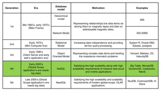
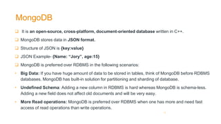
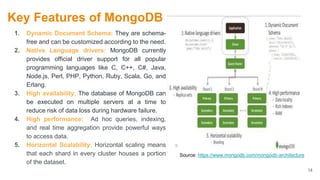
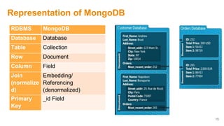
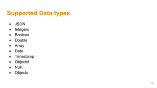
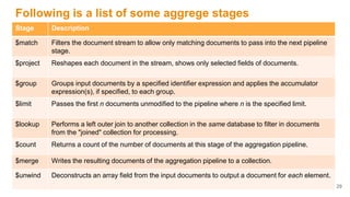
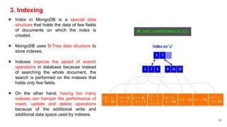
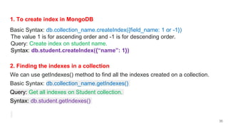
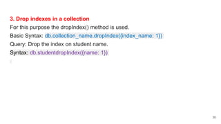
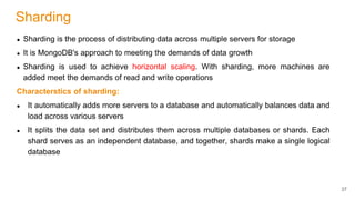
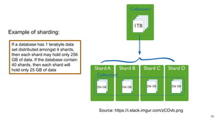
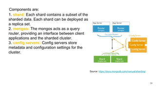
The document discusses document-oriented databases and MongoDB. It provides an overview of MongoDB, including that it is an open-source, document-based database that stores data in JSON-like documents with dynamic schemas. It supports common operations like CRUD and indexing to query and modify data efficiently. Some key features are that MongoDB is horizontally scalable, uses dynamic schemas, and is suitable for large, unstructured data like that needed in applications with big data requirements.

1. Document-Oriented Database
(MongoDB)
1

2. Index
● Introduction
○ Evolution of Database Systems
○ Introduction to NoSQL database
○ CAP theorem and BASE Property
● Document-oriented database (MongoDB)
○ Features of MongoDB
○ Use Cases of MongoDB
● Querying in MongoDB
○ CRUD operations
○ Aggregate Pipeline
○ Indexing
● Sharding in MongoDB
● References
2

3. Evaluation of database systems
3

4. 4
Generation Era
Database
model
Motivation Examples
1st
Mid 1960’s- early 1970’s
(Main Frame)
Hierarchical
model
Representing relationships b/w data items vis
storing them on magnetic tapes and later on
addressable magnetic disks.
IMS
Network Model IDS,IDMS
2nd
Early 1970’s
(Mini Computer Era)
Relational
Model
Increasing data independence and providing
ad-hoc query processing.
System R, Oracle DB2,
Sybase, postgres
3rd
Early 1980’s
(Client Server and early
web’s application era)
Object
Oriented Model
Representing complex data items and tackling
the impedance mismatch problems
Versant, Matisse, O2,
VelocityDB
4th
Early 2000’s
(Global Scope
application’s era needs
big data)
NoSQL
Satisfying the high scalability along with high
availability requirements of massive web,cloud
and mobile applications
Big Table, MongoDB,
DynamoDb, Cassandra,
Neo4j
5th
Late 2000’s (Global
Scope application’s era
needs big data)
NewSQL
Satisfying the high availability and scalability
requirements of modern global-scope, OLAP
applications.
NuoDB, CockroachDB, H-
Store

5. History of NoSQL
• In the year 1998- Carlo Strozzi use the term NoSQL for his lightweight, open-source relational database
that did not expose the standard Structured Query Language (SQL) interface.
• Big Data explosion caused organizations (large, medium and small) to seek a better way to store, manage
and analyze large unstructured data sets which was unable to handle by conventional database like
relational.
• Johan Oskarsson, reintroduced the term NoSQL in early 2009 when he organized an event to discuss
"open source distributed, non relational databases."
• It stands for 'Not Only SQL'.
Why NoSQL was developed
 To handle new requirements: Horizontal scalable, high availability, fault tolerance, transaction reliability,
database schema maintainability.
 Can handle structured, semi- structured, unstructured data.
 Flexible data models that can be schema-less.
 Relaxation on ACID property enable scaling out while achieving the high availability and low latency.
 Data can easily be replicated and horizontally partitioned across local and remote servers.
 Examples: MongoDB, Amazon Dynamo
5

6. 6
Key value
pair based
Document
based
Column
based
Graph based
e.g.Riak,
Radis etc.
Use:
Storing
session
information
e.g.
MongoDB,
CouchDB
etc.
e.g.
Cassandra ,
HBASE etc.
e.g. Neo4j,
OrientDB
etc.
Use:
e-commerce
applications
Use:
Blogging
platforms
Use:
Connections
on Social
Network

7. Terminology
Relational
database
(MySQL)
Document
based
(MongoDB)
Key-Value
based
(Riak)
Column based
(Cassandra)
Graph based
(Neo4j)
Table Collection Namespace Table Node
Row Document Key-Value Pair Row Node/Label
Column Field - Column Properties
Primary key Object_id Key Primary key -
Index Index Index Index Index
View View
-
Materialized view -
Nested table or
object
Embedded
document
-
Map Relationships
7

8. 4th generation
database
Non Relational
Distributed architecture
Open source
Horizonally Scalable 8
Features of NoSQL Database

9. Schema free
Easy replication Simple API
Can manage huge
amount of data
Can be implemented
on commodity
hardware
More than 150
NoSql databases
9

10. CAP Theorem
• Consistency: Clients should read the
same data.
• Availability: Data to be available all time.
• Partial Tolerance: Data to be partitioned
across network segments due to network
failures.
Source:https://www.researchgate.net/figure/CAP-
theorem 10

11. BASE: Basically Available, Soft State, Eventually
Consistent
Basically Available : This means that there can be a partial failure in some
parts of the distributed system and the rest of the system continues to function.
Soft State: The state of the system and data changes over time due to
eventually consistency of data.
Eventually Consistent: A possibility that the multiple copies may not be
consistent for a short period of time.
11

12. MongoDB
 It is an open-source, cross-platform, document-oriented database written in C++.
 MongoDB stores data in JSON format.
 Structure of JSON is {key:value}
 JSON Example- {Name: “Jory”, age:15}
 MongoDB is preferred over RDBMS in the following scenarios:
• Big Data: If you have huge amount of data to be stored in tables, think of MongoDB before RDBMS
databases. MongoDB has built-in solution for partitioning and sharding of database.
• Undefined Schema: Adding a new column in RDBMS is hard whereas MongoDB is schema-less.
Adding a new field does not affect old documents and will be very easy.
• More Read operations: MongoDB is preferred over RDBMS when one has more and need fast
access of read operations than write operations.
13

13. Key Features of MongoDB
1. Dynamic Document Schema: They are schema-
free and can be customized according to the need.
2. Native Language drivers: MongoDB currently
provides official driver support for all popular
programming languages like C, C++, C#, Java,
Node.js, Perl, PHP, Python, Ruby, Scala, Go, and
Erlang.
3. High availability: The database of MongoDB can
be executed on multiple servers at a time to
reduce risk of data loss during hardware failure.
4. High performance: Ad hoc queries, indexing,
and real time aggregation provide powerful ways
to access data.
5. Horizontal Scalability: Horizontal scaling means
that each shard in every cluster houses a portion
of the dataset.
Source: https://www.mongodb.com/mongodb-architecture
14

14. Representation of MongoDB
RDBMS MongoDB
Database Database
Table Collection
Row Document
Column Field
Join
(normalize
d)
Embedding/
Referencing
(denormalized)
Primary
Key
_id Field
15

15. Supported Data types
● JSON
● Integers
● Boolean
● Double
● Array
● Date
● Timestamp
● Objectid
● Null
● Objects
16

16. Use Cases of MongoDB
17

17. Case study: MongoDB with Aadhaar
● Aadhaar is India’s Unique Identification project, which has the biggest
biometrics database in the world.
● MongoDB is being used for the storage of images in the Aadhar project.
● Aadhaar chose to partner with MongoDB (in addition to other vendors such as
Hadoop, MySQL, HBase, and Solr) for several reasons.
1) MongoDB increases database efficiency with its NoSQL approach, which
enables Aadhaar to capture, process, search, and analyze large unstructured
datasets faster than most other management softwares.
2) MongoDB can efficiently store large volumes of biometric data and images,
whereas many other management systems, such as MySQL, are less suited for
image storage.
18

18. Sample Database (“Studentinfo”)
{
"_id" : ObjectId("61f6f4e0dd0c8af093eb9255"),
"studentName" : "Gaurav",
"section" : "A",
"Marks" : 90,
"subject" : [
"English"
]
}
{
"_id" : ObjectId("61f6f4e0dd0c8af093eb9254"),
"studentName" : "Vijay",
"section" : "A",
"Marks" : 70,
"subject" : [
"Hindi",
"English",
"Math"
]
}
Collection
(“Student”)
Document 1
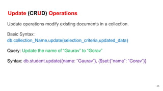
Document 2
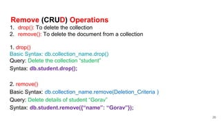
19
.
.
.
.
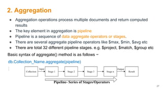
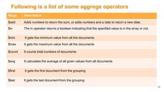
Document n
Fields
Fields
Primary
key
Primary
key
Embedded/Nested
documents

19. Querying in MongoDB
1. CRUD (Create, Read, Update, Delete) operations: These functions can be
broadly classified as data modification functions in MongoDB. These can only be
used for a single collection.
2. Aggregation:
● Process data records and return computed results. It can be applied on
multiple douments. Includes Operators like $sum, $max, $min etc.
● Aggregation pipeline method is used to perform the aggregations. Includes
Stages like $match, $project and many more.
3. Indexing: Used to make queries performance more efficient. It includes:
a) Create index b) Find Index 3) Drop Index
20

20. 1. MongoDB CRUD Operations
Create (CRUD) Operations:
It includes
1) create() : Creation of new collection
2) insert() : insertion of one or more documents inside a collection
It includes two other methods:
● insertone(): To insert one document inside a collection
● insertmany(): To insert many docuemnts inside a collection
21

21. 1. create()
Basic Syntax: db.createCollection(name, options)
Query: Create a new collection “student”
Syntax: db.createCollection(“student”);
2. insert(): The insert() method is used to insert one or multiple documents in a
collection.
Basic Syntax: db.collection_Name.insert(JSON document)
Query: Insert the marks of a students named ‘Vijay, Gaurav’ in section ‘A’ having
subjects ‘Hindi, English, Math’,and ‘English’ respectively.
Syntax: db.student.insert ({studentName: “Vijay”, section: “A”, Marks: 70, subject:
[“Hindi”, “English”, “Math”]})
db.student.insert[{studentName: “Gaurav”, section: “A”, Marks: 90, subject:
[“English”]}])
22

22. 2. insertOne(): Another way to insert documents is by using the insertOne()
method for a single document in a collection.
Basic Syntax: db.collection_Name.insertone(JSON document)
Query: Insert the marks of a student named ‘Vijay’ in section ‘A’ having subjects
‘Hindi, English, Math’.
Syntax: db.student.insert ({studentName: “Vijay”, section: “A”, Marks: 70, subject:
[“Hindi”, “English”, “Math”]})
3. insertMany(): is used for inserting multiple documents:
Basic Syntax: db.collection_Name.insertmany([array of JSON document])
Query: Insert the marks of a students named ‘Vijay, Gaurav’ in section ‘A’ having
subjects ‘Hindi, English, Math’,and ‘English’ respectively.
Syntax: db.student.insertMany( [ { studentName: “Vijay”, section: “A”, Marks: 70,
subject: [“Hindi”, “English”, “Math”]}, { studentName: “Gaurav”, section: “A”,
Marks: 90, subject: [“English”]}]);
23

23. Read (CRUD) Operations
Read operations retrieves documents from a collection; i.e. queries a
collection for documents.
Basic syntax: db.collection.find()
Query: Display the details of students
Syntax: db.student.find{};
pretty(): This method is used for giving a proper format to the output
extracted by the query.
Basic Syntax: db.collection.find().pretty();
Query: Display the details of students
Syntax: db.student.find().pretty();
24

24. Update (CRUD) Operations
Update operations modify existing documents in a collection.
Basic Syntax:
db.collection_Name.update(selection_criteria,updated_data)
Query: Update the name of “Gaurav” to “Gorav”
Syntax: db.student.update({name: “Gaurav”}, {$set:{“name”: “Gorav”}}
25

25. Remove (CRUD) Operations
1. drop(): To delete the collection
2. remove(): To delete the document from a collection
1. drop()
Basic Syntax: db.collection_name.drop()
Query: Delete the collection “student”
Syntax: db.student.drop();
2. remove()
Basic Syntax: db.collection_name.remove(Deletion_Criteria )
Query: Delete details of student “Gorav”
Syntax: db.student.remove({“name”: “Gorav”});
26

26. 2. Aggregation
● Aggregation operations process multiple documents and return computed
results
● The key element in aggregation is pipeline
● Pipeline is a sequence of data aggregate operators or stages.
● There are several aggregate pipeline operators like $max, $min, $avg etc
● There are total 32 different pipeline stages. e.g. $project, $match, $group etc
Basic syntax of aggregate() method is as follows −
db.Collection_Name.aggregate(pipeline)
27

27. Following is a list of some aggrege operators
28
Stage Description
$add Adds numbers to return the sum, or adds numbers and a date to return a new date.
$in The in operator returns a boolean indicating that the specified value is in the array or not.
$min It gets the minimum value from all the documents
$max It gets the maximum value from all the documents
$count It counts total numbers of documents
$avg It calculates the average of all given values from all documents
$first It gets the first document from the grouping
$last It gets the last document from the grouping

28. Following is a list of some aggrege stages
29
Stage Description
$match Filters the document stream to allow only matching documents to pass into the next pipeline
stage.
$project Reshapes each document in the stream, shows only selected fields of documents.
$group Groups input documents by a specified identifier expression and applies the accumulator
expression(s), if specified, to each group.
$limit Passes the first n documents unmodified to the pipeline where n is the specified limit.
$lookup Performs a left outer join to another collection in the same database to filter in documents
from the "joined" collection for processing.
$count Returns a count of the number of documents at this stage of the aggregation pipeline.
$merge Writes the resulting documents of the aggregation pipeline to a collection.
$unwind Deconstructs an array field from the input documents to output a document for each element.

29. Examples
Following are the three popular stages in aggregation framework:
1) $match − This is a filtering operation and thus this can reduce the amount of
documents that are given as input to the next stage.
Basic Syntax: { $match: { <query> } }
Query 1: Display the details of students belong to section “A”
Syntax: db.student.aggregate([{“$match:{“section”: “A”}}])
Query 2: Display the details of students belong to section “A” and marks greater
than 80
db.student.aggregate([{“$match”: { $and:[{“section”: “A”}, {Marks:
{“$gt”: 80}}]}}])
30

30. 31
2) $project − Used to select some specific fields from a collection.
Basic Syntax:
Query 1: Display name, section and marks of all the students.
Syntax: db.student.aggregate([{“$project”: {studentName: 1, section: 1,
Marks: 1}}])
Query 2: Display the names and marks of students from section A.
Syntax: db.student.aggregate([{$match:{“section”: “A”}}, {“$project”:
{studentName: 1, Marks:1}}])
{ $project: { <specification(s)> } }

31. 3) $group − This does the actual aggregation as discussed above.
Basic Syntax:
{ $group: { _id: <expression>, // Group By Expression <field1>: { <accumulator1> :
<expression1> },}}
Query 1: To find out total marks each section.
Syntax: db.student.aggregate([{“$group”:{“_id”: {“section : “$section”}, “Total
Marks”:{“$sum”: “$Marks”}}}])
Query 2: To find the total marks of section A.
Syntax: db.student.aggregate([{“$match”: {section: ‘A’}}, {“$group”:{“_id”: {“section :
“$section”}, “Total Marks”:{“$sum”: “$Marks”}}}])
32

32. Query 3: To find total and average marks of each section.
Syntax: db.student.aggregate([{“$group”:{“_id”: {“section : “$section”}, “Total
Marks”:{“$sum”: “$Marks”}, “Count”:{ “$sum”:1}, “Average”: {“$avg”: “$Marks”}}}])
33

33. 3. Indexing
● Index in MongoDB is a special data
structure that holds the data of few fields
of documents on which the index is
created.
● MongoDB uses B-Tree data structure to
store indexes.
● Indexes improve the speed of search
operations in database because instead
of searching the whole document, the
search is performed on the indexes that
holds only few fields.
● On the other hand, having too many
indexes can hamper the performance of
insert, update and delete operations
because of the additional write and
additional data space used by indexes.
34

34. 1. To create index in MongoDB
Basic Syntax: db.collection_name.createIndex({field_name: 1 or -1})
The value 1 is for ascending order and -1 is for descending order.
Query: Create index on student name.
Syntax: db.student.createIndex({“name”: 1})
2. Finding the indexes in a collection
We can use getIndexes() method to find all the indexes created on a collection.
Basic Syntax: db.collection_name.getIndexes()
Query: Get all indexes on Student collection.
Syntax: db.student.getIndexes()
35

35. 3. Drop indexes in a collection
For this purpose the dropIndex() method is used.
Basic Syntax: db.collection_name.dropIndex({index_name: 1})
Query: Drop the index on student name.
Syntax: db.studentdropIndex({name: 1})
36

36. Sharding
● Sharding is the process of distributing data across multiple servers for storage
● It is MongoDB's approach to meeting the demands of data growth
● Sharding is used to achieve horizontal scaling. With sharding, more machines are
added meet the demands of read and write operations
Characterstics of sharding:
● It automatically adds more servers to a database and automatically balances data and
load across various servers
● It splits the data set and distributes them across multiple databases or shards. Each
shard serves as an independent database, and together, shards make a single logical
database
37

37. Example of sharding:
38
If a database has 1 terabyte data
set distributed amongst 4 shards,
then each shard may hold only 256
GB of data. If the database contain
40 shards, then each shard will
hold only 25 GB of data
Source: https://i.stack.imgur.com/zCOvb.png

38. Components are:
1. shard: Each shard contains a subset of the
sharded data. Each shard can be deployed as
a replica set.
2. mongos: The mongos acts as a query
router, providing an interface between client
applications and the sharded cluster.
3. config servers: Config servers store
metadata and configuration settings for the
cluster.
Source: https://docs.mongodb.com/manual/sharding/
39

39. References
1. MongoDB website, https://www.mongodb.com
2. Dan Sullivan. “Nosql for mere Mortals”,1st Edition,United States of America:Pearson
Education,2015.
3. “Top 5 considerations when evaluating NoSql databases”,MongoDB white paper,2015.
(https://www.mongodb.com/collateral/top-5-considerations-when-evaluating-nosql-databases).
4. Davoudian, Ali, Liu Chen, and Mengchi Liu. “A survey on NoSQL stores.” ACM Computing Surveys
(CSUR) 51, no. 2 (2018): 1-43
5. Cattell, R. “Scalable SQL and NoSQL data stores.” Acm Sigmod Record, 39(4), pp.12-27, 2015.
6. Floratou, Avrilia, Nikhil Teletia, David J. DeWitt, Jignesh M. Patel, and Donghui Zhang. "Can the
Elephants Handle the NoSQL Onslaught?." Proceedings of the VLDB Endowment 5, no. 12 (2012).
7. Patel, Jignesh M. "Operational NoSQL Systems: What's New and What's Next?." Computer 49, no.
4 (2016): 23-30.
8. Abadi, Daniel, Rakesh Agrawal, Anastasia Ailamaki, Magdalena Balazinska, Philip A. Bernstein,
Michael J. Carey, Surajit Chaudhuri et al. "The Beckman report on database
research." Communications of the ACM 59, no. 2 (2016): 92-99.
40