Download as PDF, PPTX


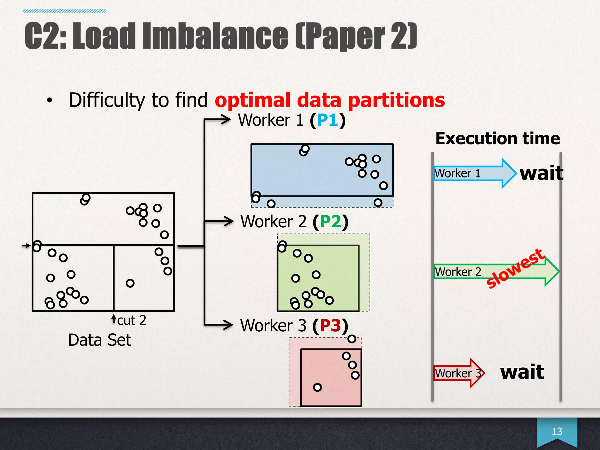


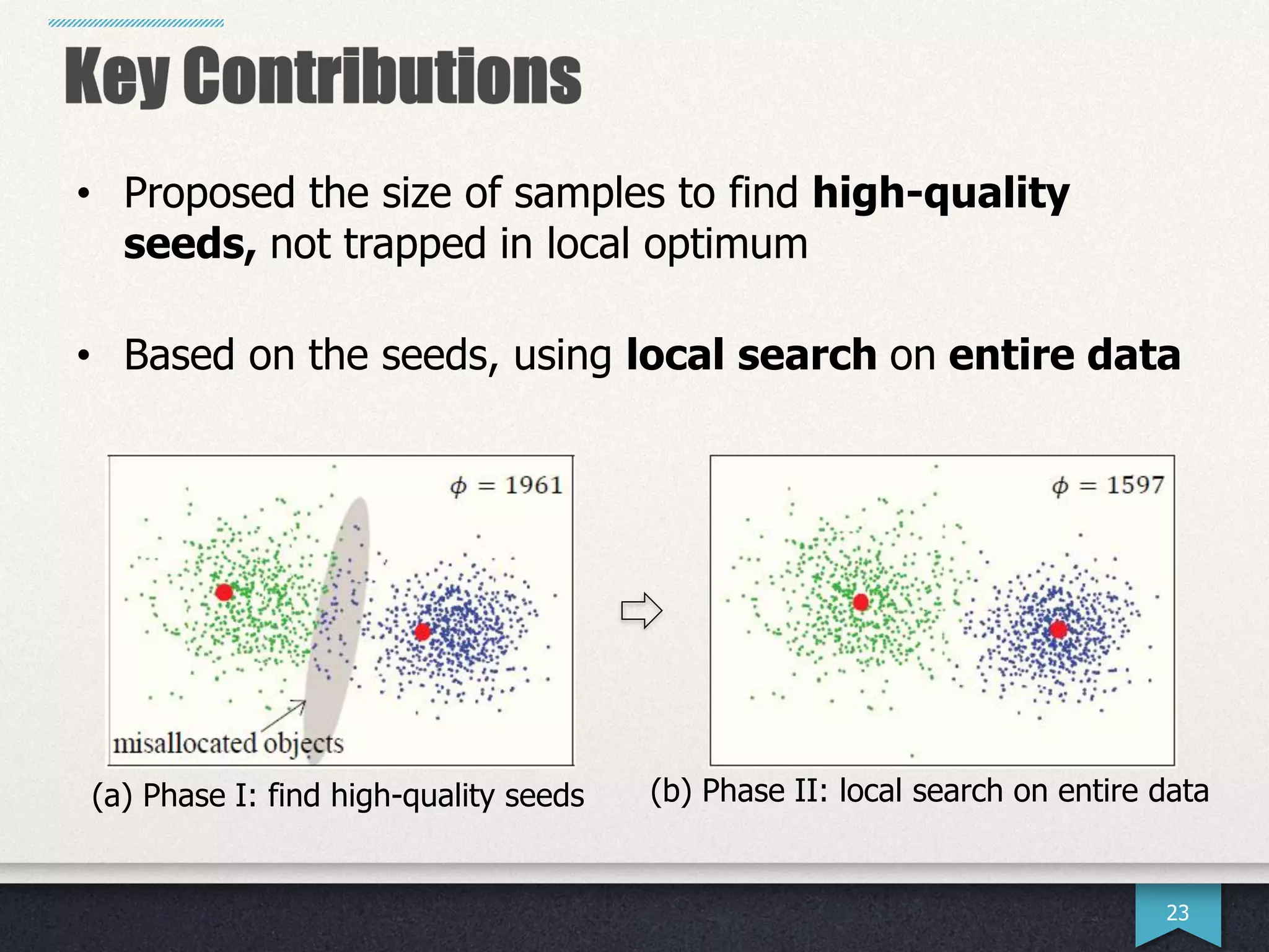


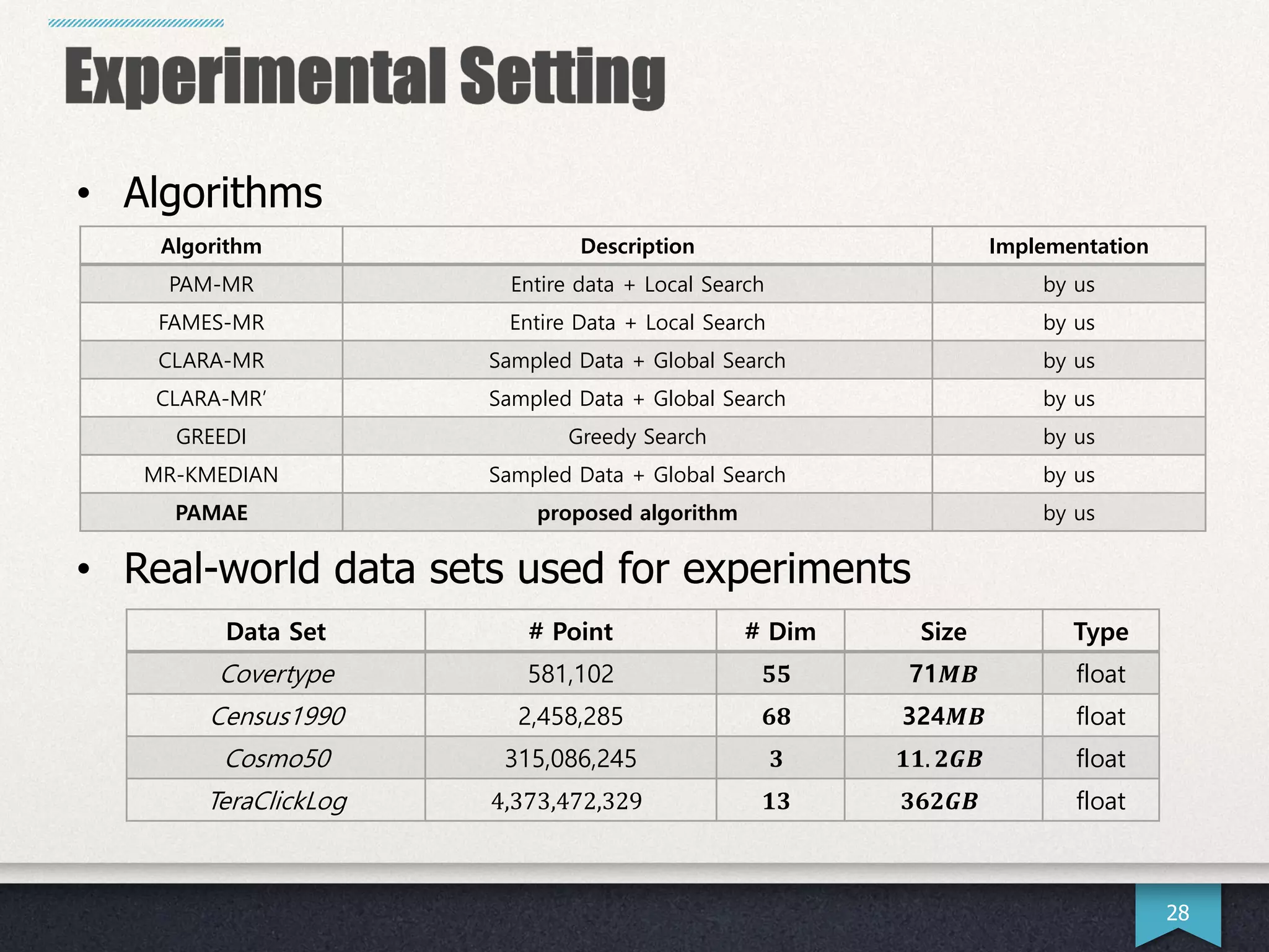
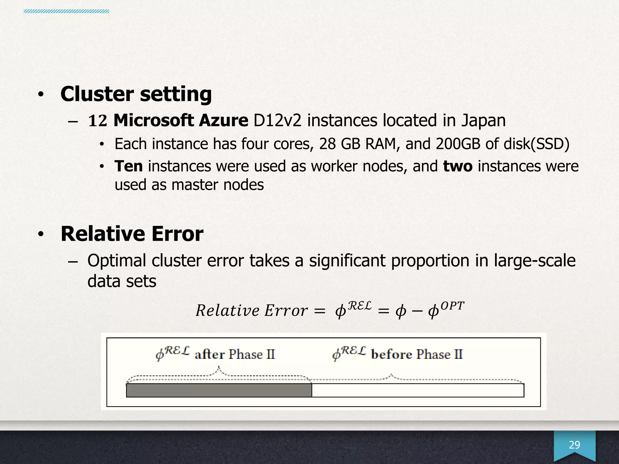
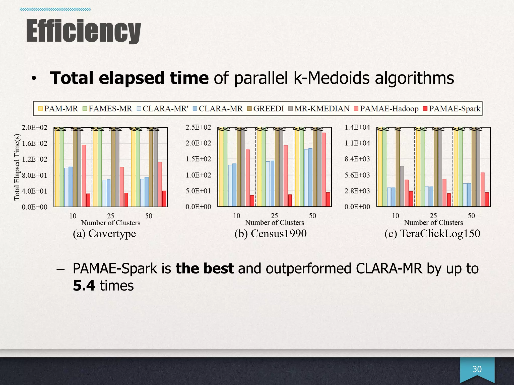


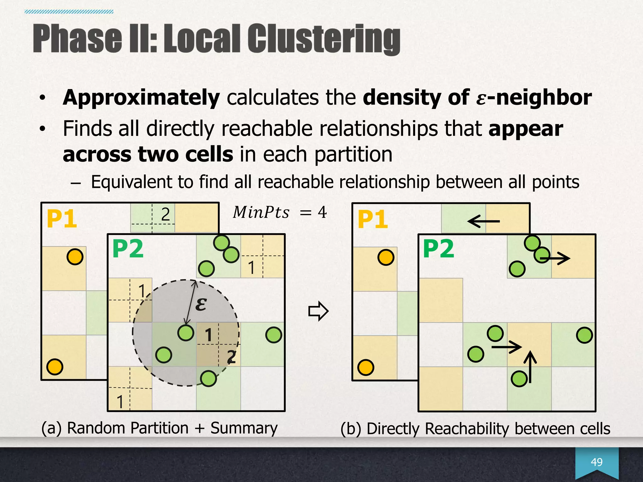


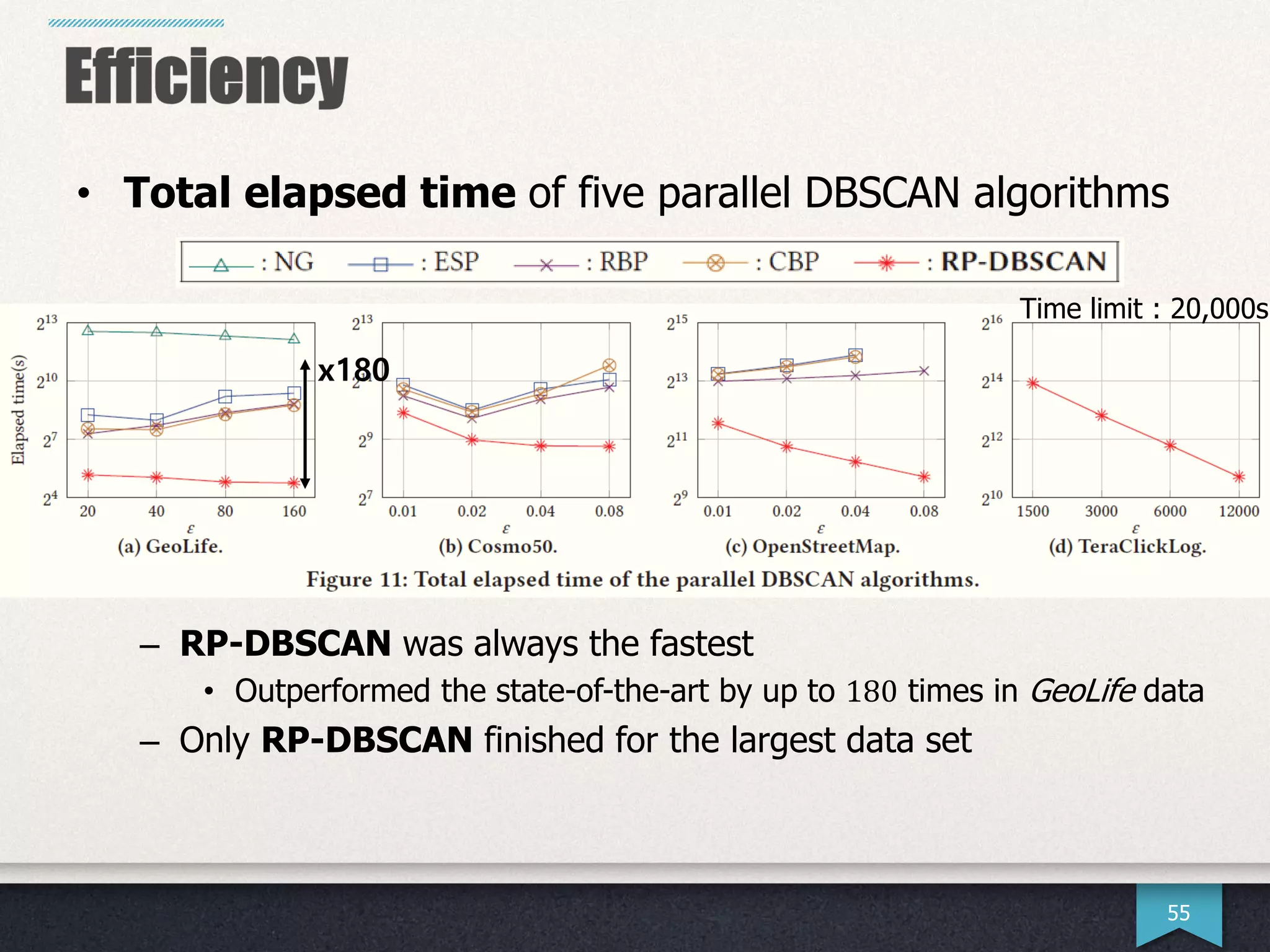
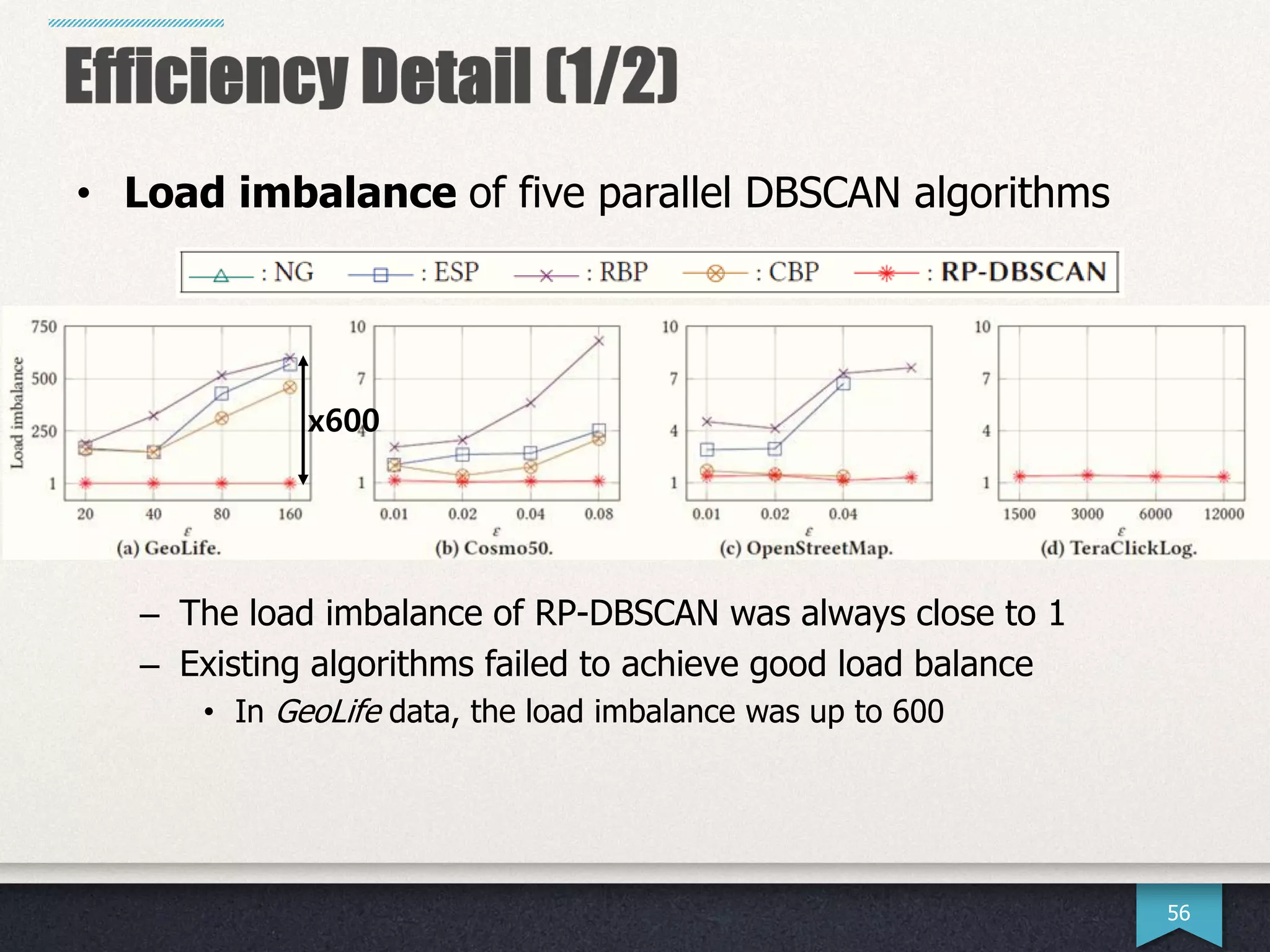


The document presents research by Hwanjun Song on optimizing parallel clustering algorithms for large-scale data analytics, particularly focusing on k-medoids and the newly proposed PAMAe algorithm. It details issues with existing methods, such as high computational complexity and accuracy trade-offs, and introduces a random partitioning approach to improve efficiency and balance in processing. Experimental results demonstrate that PAMAe significantly outperforms traditional methods, achieving greater accuracy while reducing computational costs.


![Vibe Coding vs. Spec-Driven Development [Free Meetup]](https://cdn.slidesharecdn.com/ss_thumbnails/vibecodingvsspecdrivendevelopment-251209105622-43f455e7-thumbnail.jpg?width=640&height=640&fit=bounds)


