Thermodynamics

1. Production of Power
from Heat

2. Introduction
• Work can readily be transformed into other forms of energy (such as
heat); however, converting heat to work cannot be done easily
• Heat engines are special devices or machines that produce work from
heat in a cyclic process

3. Introduction
• A power cycle is one where heat is absorbed by the fluid, and
transformed into work, with the remaining heat rejected
• To facilitate power cycles, a working fluid is needed, which absorbs
heat from a heat reservoir, produces a net amount of work ,
discards heat to a cold reservoir, and returns to its initial state

4. Introduction
• This chapter is devoted to the analysis of several common heat
engine cycles
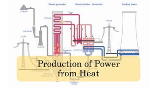
SIMPLE STEAM
POWER PLANT

5. Power Cycles
• Power cycles can be categorized depending upon the working fluid used:
Vapor power cycle- working fluid exists in vapor phase during one part of the
cycle, and in liquid phase during another part of the cycle
- fluid undergoes a thermodynamic cycle
Gas power cycle- working fluid remains in the gaseous phase throughout the
entire cycle
- mechanical cycle: fluid may start as a liquid, then exhausted
as a mixture of combustion gases

6. The Carnot Cycle
• Carnot cycle- the most efficient heat engine cycle allowed by physical
laws
• The Carnot efficiency sets the limiting value on the fraction of the
heat which can be used:
(note: the magnitude, not the sign, is important.)

7. The Carnot Cycle
• The cycle consists of four processes:
 Reversible isothermal absorption of heat from a heat source at a high
temperature
 Reversible adiabatic (isentropic) expansion: the system is thermally
insulated; the fluid expands from boiler pressure at to the condenser
pressure at , and produces work

8. The Carnot Cycle
• The cycle consists of four processes (continued):
 Reversible isothermal rejection of heat at
A reversible adiabatic (isentropic) compression: the system is thermally
insulated; the fluid compresses from condenser pressure at to the boiler
pressure at ; work is done on the fluid

9. The Carnot Cycle
Step Equipment Process
b-c Boiler Reversible Isothermal Absorption
of Heat
c-d Turbine Reversible Adiabatic (Isentropic)
Expansion
d-a condenser Reversible Isothermal Rejection
of Heat
a-d Pump Reversible Adiabatic (Isentropic)
Compression

10. The Carnot Cycle
Step Equipment Process
1-2 Boiler Reversible Isothermal Absorption
of Heat
2-3 Turbine Reversible Adiabatic (Isentropic)
Expansion
3-4 Condenser Reversible Isothermal Rejection
of Heat
4-1 Pump Reversible Adiabatic (Isentropic)
Compression

11. Illustrative Problem
Saturated liquid in a power plant is boiled isothermally to saturated
vapor, and is fed to a turbine at a pressure of 7231.5 kPa and a
temperature of 561.15K. Exhaust from the turbine enters a condenser
at a pressure 10.09 kPa and a temperature of 319.15K, which is then
pumped to the boiler.
Find: , , , , , and .

12. Solving Problems Involving Cycles
A step-by-step approach in solving problems involving thermodynamic
cycles is as follows:
1. Draw the schematic diagram of the power plant
2. Draw a T-S diagram and put appropriate labels
3. Make a table listing down relevant properties
4. Write energy and entropy balances around the equipment used in
the plant
5. Solve for the variables of interest (shaft work, efficiency of the
cycle, entropy generation)

13. Schematic Diagram
• Before solving the problem,
sketching a schematic diagram is
done in order to visualize the
cycle
• The flows are assigned numbers;
said flows are at a certain state
• Draw the equipment and label
appropriately

14. T-S Diagram
• The T-S diagram plots the specific entropy of the fluid against
temperature
• This diagram is useful in visualizing how the cycle operates. For
example:
 the points where the fluid will undergo a phase change,
 the areas under the curves, which pertain to the heat absorbed (using a
boiler) and heat rejected (using a condenser), and
 the points where the fluid is a two-phase mixture

15. Drawing a T-S Diagram
Start with a “blank” diagram:

16. Drawing a T-S Diagram
Draw the relevant isobars:

17. Drawing a T-S Diagram
Label intersection of the isobar PTH and the saturated liquid curve as state (1):

18. Drawing a T-S Diagram
Label intersection of the isobar PTH and the saturated vapor curve as state (2); draw an arrow from (1) to (2):

19. Drawing a T-S Diagram
Draw an arrow perpendicular to arrow (1)-(2), from (2) until it intersects the isobar PTC ; label the intersection as state (3):

20. Drawing a T-S Diagram
Draw an arrow from (3) until it intersects the "line” perpendicular to arrow (1)-(2) ; label the point as state (4):

21. Drawing a T-S Diagram
Draw an arrow from (4) to (1) to complete the cycle; label accordingly:

22. Drawing a T-S Diagram
Animation:

23. Table of Property Data
A good way to organize the property data from the steam tables is by
making a table of property data. The format of this table is as follows:
Point State P(kPa) T(K) H(kJ kg-1) S(kJ kg-1 K-1) Quality (x)
1 Saturated Liquid 7231.5 561.15 1279.2 3.1424 -
2 Saturated Vapor 7231.5 561.15 2770.5 5.7997 1
3 Saturated Vapor 10.09 319.15 1835.6 5.7997 0.6867
4 Saturated Liquid 10.09 319.15 987.5 3.1424 0.3323

24. Quality
• Recall that, in the T-S diagram, points (3) and (4) do not lie along the
saturated vapor-liquid curve; instead, they lie inside the dome
• In order to solve for the properties of these points, one must first
consider the quality of the steam

25. Quality
• The quality of the steam is defined to be the mass fraction of a
vapor/liquid mixture that is vapor:
𝑥 =
𝑚𝑣𝑎𝑝
𝑚𝑚𝑖𝑥𝑡𝑢𝑟𝑒
• Relevant equations:
1) 𝑆𝑚𝑖𝑥𝑡𝑢𝑟𝑒 = 𝑆𝑠𝑎𝑡𝑙𝑖𝑞 + 𝑥(𝑆𝑠𝑎𝑡𝑣𝑎𝑝 − 𝑆𝑠𝑎𝑡𝑙𝑖𝑞)
2) 𝐻𝑚𝑖𝑥𝑡𝑢𝑟𝑒 = 𝐻𝑠𝑎𝑡𝑙𝑖𝑞 + 𝑥(𝐻𝑠𝑎𝑡𝑣𝑎𝑝 − 𝐻𝑠𝑎𝑡𝑙𝑖𝑞)
3) 𝑉𝑚𝑖𝑥𝑡𝑢𝑟𝑒 = 𝑉𝑠𝑎𝑡𝑙𝑖𝑞 + 𝑥(𝑉𝑠𝑎𝑡𝑣𝑎𝑝 − 𝑉𝑠𝑎𝑡𝑙𝑖𝑞)

26. Quality
• The quality of steam can be computed using one of these equations;
choosing what equation to use will depend on what particular
properties are given
• In the case of the Carnot cycle, equation (1) is commonly used (for
example, in an isentropic expansion process, 𝑆2 = 𝑆3; hence, 𝑆2 is the
𝑆𝑚𝑖𝑥𝑡𝑢𝑟𝑒 at (3))

27. Quality
x = Quality of Steam
x =
𝑀𝑎𝑠𝑠 𝑜𝑓 𝑆𝑎𝑡𝑢𝑟𝑎𝑡𝑒𝑑 𝑉𝑎𝑝𝑜𝑟 𝑖𝑛 𝑊𝑒𝑡 𝑉𝑎𝑝𝑜𝑟
𝑀𝑎𝑠𝑠 𝑜𝑓 𝑤𝑒𝑡 𝑣𝑎𝑝𝑜𝑟
y =
𝑀𝑎𝑠𝑠 𝑜𝑓 𝑆𝑎𝑡𝑢𝑟𝑎𝑡𝑒𝑑 𝑙𝑖𝑞𝑢𝑖𝑑 𝑖𝑛 𝑊𝑒𝑡 𝑉𝑎𝑝𝑜𝑟
𝑀𝑎𝑠𝑠 𝑜𝑓 𝑤𝑒𝑡 𝑣𝑎𝑝𝑜𝑟
Sat’d liquid
Sat’d vapor
S
𝑆𝑙𝑖𝑞𝑢𝑖𝑑
𝑆𝑣𝑎𝑝𝑜𝑟
𝑆𝑣𝑎𝑝𝑜𝑟 - 𝑆𝑙𝑖𝑞𝑢𝑖𝑑
x y
𝑥 =
𝑆 − 𝑆𝑙𝑖𝑞𝑢𝑖𝑑
𝑆𝑣𝑎𝑝𝑜𝑟 − 𝑆𝑙𝑖𝑞𝑢𝑖𝑑
S = 𝑆𝑙𝑖𝑞𝑢𝑖𝑑 + 𝑥(𝑆𝑣𝑎𝑝𝑜𝑟 − 𝑆𝑙𝑖𝑞𝑢𝑖𝑑)

28. Property Data
Point State P(kPa) T(K) H(kJ kg-1) S(kJ kg-1 K-1) Quality (x)
1 Saturated Liquid 7231.5 561.15 1279.2 3.1424 -
2 Saturated Vapor 7231.5 561.15 2770.5 5.7997 1
3 Wet Vapor 10.09 319.15 1835.6 5.7997 0.6867
4 Wet Vapor 10.09 319.15 987.5 3.1424 0.3323
𝑥3 =
𝑆2 − 𝑆𝑠𝑎𝑡𝑙𝑖𝑞,319.15𝐾
𝑆𝑠𝑎𝑡𝑣𝑎𝑝,319.15𝐾 − 𝑆𝑠𝑎𝑡𝑙𝑖𝑞,319.15𝐾
=
5.7997 − 0.6514
8.1481 − 0.6514
= 0.6867
Calculations (values taken from steam tables):
𝑥4 =
𝑆1 − 𝑆𝑠𝑎𝑡𝑙𝑖𝑞,319.15𝐾
𝑆𝑠𝑎𝑡𝑣𝑎𝑝,319.15𝐾 − 𝑆𝑠𝑎𝑡𝑙𝑖𝑞,319.15𝐾
=
3.1424 − 0.6514
8.1481 − 0.6514
= 0.3323
H3 = 𝐻𝑠𝑎𝑡𝑙𝑖𝑞,319.15 + 𝑥3(𝐻𝑠𝑎𝑡𝑣𝑎𝑝,319.15𝐾 - 𝐻𝑠𝑎𝑡𝑙𝑖𝑞,319.15𝐾 )
H3 = 192.5 + (0.6867)(2585.1- 192.5)
H3 = 1835.6 𝑘𝐽 𝑘𝑔−1
H4 = 𝐻𝑠𝑎𝑡𝑙𝑖𝑞,319.15 + 𝑥4(𝐻𝑠𝑎𝑡𝑣𝑎𝑝,319.15𝐾 - 𝐻𝑠𝑎𝑡𝑙𝑖𝑞,319.15𝐾 )
H3 = 192.5 + (0.3323)(2585.1- 192.5)
H3 = 987. 5 𝑘𝐽 𝑘𝑔−1

29. Energy Balance
• We will now use the properties in the table in order to solve for the
quantities of interest (shaft work, efficiency, etc.)
• One way to solve for these quantities is by writing energy balances
around the equipment used

30. Energy Balance: Boiler
Assumptions: no work done; potential and kinetic energy effects are
ignored
Energy Balance:
Δ𝑃𝐸 + Δ𝐾𝐸 + Δ𝐻 = 𝑊
𝑠 + 𝑄𝐻
→ Δ𝐻 = 𝑄𝐻
0 0 0

31. Energy Balance: Turbine
Assumptions: adiabatic; potential and kinetic energy effects are ignored
Energy Balance:
Δ𝑃𝐸 + Δ𝐾𝐸 + Δ𝐻 = 𝑊
𝑠 + 𝑄
→ Δ𝐻 = 𝑊
𝑠(𝑡𝑢𝑟𝑏𝑖𝑛𝑒)
0 0 0

32. Energy Balance: Condenser
Assumptions: no work done; potential and kinetic energy effects are
ignored
Energy Balance:
Δ𝑃𝐸 + Δ𝐾𝐸 + Δ𝐻 = 𝑊
𝑠 + 𝑄𝐶
→ Δ𝐻 = 𝑄𝐶
0 0 0

33. Energy Balance: Pump
Assumptions: adiabatic; potential and kinetic energy effects are ignored
Energy Balance:
Δ𝑃𝐸 + Δ𝐾𝐸 + Δ𝐻 = 𝑊
𝑠 + 𝑄
→ Δ𝐻 = 𝑊
𝑠(𝑝𝑢𝑚𝑝)
0 0 0

34. Solving for Shaft Work (For a Turbine and Pump)
Writing the energy balance of the turbine,
𝑊
𝑠 𝑡𝑢𝑟𝑏𝑖𝑛𝑒 = Δ𝐻 = 𝐻3 − 𝐻2
= 1835.6 − 2770.5 𝑘𝐽 𝑘𝑔−1
= −934.9 𝑘𝐽 𝑘𝑔−1.
Writing the energy balance of the pump,
𝑊
𝑠 𝑝𝑢𝑚𝑝 = Δ𝐻 = 𝐻1 − 𝐻4
= 1279.2 − 987.5 𝑘𝐽 𝑘𝑔−1
= 291.7 𝑘𝐽 𝑘𝑔−1.
→ 𝑊𝑛𝑒𝑡 = −934.9 + 291.7 𝑘𝐽 𝑘𝑔−1
= −643.2 𝑘𝐽 𝑘𝑔−1
Note: the energy balances used
for the turbine and pump are for
open systems.

35. Solving for QH and QC
Writing the energy balance of the boiler,
𝑄𝐻 = Δ𝐻 = 𝐻2 − 𝐻1
= 2770.5 − 1279.2 𝑘𝐽 𝑘𝑔−1
= 1491.3 𝑘𝐽 𝑘𝑔−1
Writing the energy balance of the condenser,
𝑄𝐶 = Δ𝐻 = 𝐻3 − 𝐻2
= 987.5 − 1835.6 𝑘𝐽 𝑘𝑔−1
= −848.1 𝑘𝐽 𝑘𝑔−1
By the 1st law of thermodynamics for closed systems (cycle),
→ |𝑄𝐻| − |𝑄𝐶| = 𝑊
𝑠(𝑛𝑒𝑡) = 1491.3 − 848.1 𝑘𝐽 𝑘𝑔−1
= 643.2 𝑘𝐽 𝑘𝑔−1
Note: the energy balances used
for the boiler and condenser are
for open systems.

36. Solving for QH and QC
• |𝑄𝐻|, |𝑄𝐶| and |𝑊
𝑠 𝑛𝑒𝑡 | can be solved by evaluating the areas under
the curves in the T-S diagram
• For the boiler, |𝑄𝐻| = 𝑇𝐻 𝑆2 − 𝑆1 = 𝑇𝐻 𝑆3 − 𝑆4
• For the condenser, |𝑄𝐶| = 𝑇𝐶 𝑆2 − 𝑆1 = 𝑇𝐶 𝑆3 − 𝑆4
• Solving for 𝑊
𝑠 𝑛𝑒𝑡 : |𝑊
𝑠 𝑛𝑒𝑡 | = 𝑇𝐻 − 𝑇𝐶 𝑆2 − 𝑆1
= (𝑇𝐻 − 𝑇𝐶) 𝑆3 − 𝑆4

37. Solving for QH and QC
Illustration:

38. Solving for QH and QC

39. Solving for QH and QC

40. Solving for QH and QC
|𝑄𝐻| = 561.15 𝐾 5.7997 − 3.1424 𝑘𝐽 𝑘𝑔−1 𝐾−1
= 1491.14 𝑘𝐽 𝑘𝑔−1
|𝑄𝐶| = 319.15 𝐾 5.7997 − 3.1424 𝑘𝐽 𝑘𝑔−1 𝐾−1
= 848.08 𝑘𝐽 𝑘𝑔−1
|𝑊
𝑠 𝑛𝑒𝑡 | = 561.15 𝐾 − 319.15𝐾 5.7997 − 3.1424 𝑘𝐽 𝑘𝑔−1 𝐾−1
= 643.06 𝑘𝐽 𝑘𝑔−1

41. Solving for Carnot Efficiency
𝜂 = 1 −
319.15 𝐾
561.15 𝐾
= 0.4313
Or…
𝜂 =
|𝑊
𝑠 𝑛𝑒𝑡 |
|𝑄𝐻|
=
643.06 𝑘𝐽 𝑘𝑔−1
1491.14 𝑘𝐽 𝑘𝑔−1
= 0.4313

42. Thank you!