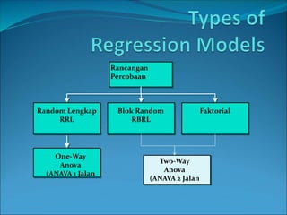
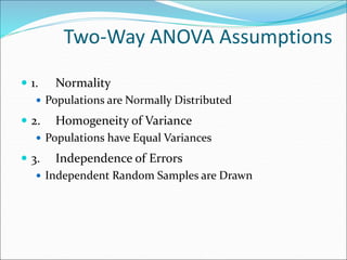
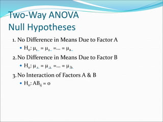
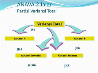
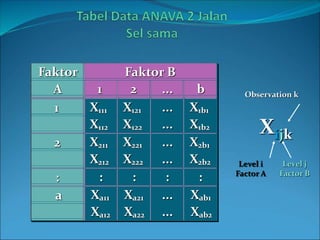
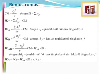
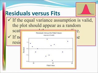
“Nikmat manakah yang kamu dustakan? “
Review
Analisis Variansi dan Efek Utama
• Analisis variansi dengan 1 efek utama dikenal sebagai
analisis variansi satu jalan
• Analisis variansi dengan 2 efek utama dikenal sebagai
analisis variansi dua jalan
• Analisis variansi dengan 3 efek utama dikenal sebagai
analisis variansi tiga jalan
• Dan demikian seterusnya
 Analisis variansi satu jalan hanya terdiri atas satu faktor
dengan dua atau lebih level
 Analisis variansi dua jalan terdiri atas dua faktor, masing-
masing dengan dua atau lebih level
 Faktor menghasilkan efek utama sehingga di sini
terdapat dua efek utama
Faktor Utama dan Interaksi
 Dalam hal lebih dari satu faktor, faktor itu dapat saja saling
mempengaruhi atau tidak saling mempengaruhi
 Apabila faktor itu tidak saling mempengaruhi maka kita memperoleh
dua faktor utama saja
 Apabila faktor itu saling mempengaruhi, maka selain efek utama,
kita memperoleh lagi interaksi pada saling mempngaruhi itu
 Dalam hal terdapat interaksi, kita memiliki efek utama dan interaksi
• Efek utama (dengan perbedaan rerata)
• Interaksi (dengan interaksi di antara faktror)
Variansi dan Efek Utama
Variansi sebelum ada efek
Variansi antara kelompok
Kelompok 1 (level 1)
Kelompok 2 (level 2)
Kelompok 3 (level 3)
Ada variansi dalam
kelompok pada kelompok
masing-masing
Ada variansi antara
kelompok
Variansi Sesudah Ada Efek Utama
Variansi antara kelompok
Variansi dalam kelompok tidak berubah
Variansi antara kelompok
menjadi besar:
Ada efek,
Paling sedikit ada satu
pasang rerata yang beda









Variansi Total
Variansi total
Dengan membuka batas semua
kelompok, diperoleh variansi total









So …Sources of variance
 When we take samples from each population,
there will be two sources of variability
 Within group variability - when we sample from a group
there will be variability from person to person in the
same group  Sesatan
 We will always have this form of variability because it is sampling
variability
 Between group variability – the difference from group to
group  Perlakuan
 This form of variability will only exist if the groups are different
 If the between group variability if large, the means of the two
groups is likely not the same
 We can use the two types of variability to determine
if the means are likely different
 How can we do this?
 Look again at the picture
 Blue arrow: within group, red arrow: between group
Rancangan
Percobaan
One-Way
Anova
(ANAVA 1 Jalan
Random Lengkap
RRL
Blok Random
RBRL
Two-Way
Anova
(ANAVA 2 Jalan
Faktorial
 Eksperimen faktorial a x b melibatkan 2 faktor dimana
terdapat a tingkat faktor A dan b tingkat faktor B,
 Eksperimen diulang r kali pada tiap-tiap tingkat faktor
kombinasi
 Adanya replikasi inilah yang memungkinkan
terjadinya interaksi antara faktor A dan B
Rancangan Faktorial a x b
Interaction
 Occurs When Effects of One Factor Vary According to Levels
of Other Factor
 When Significant, Interpretation of Main Effects (A & B) Is
Complicated
 Can Be Detected
In Data Table, Pattern of Cell Means in One Row Differs
From Another Row
In Graph of Cell Means, Lines Cross
 The interaction between two factor A and B is the tendency
for one factor to behave differently, depending on the
particular level setting of the other variable.
 Interaction describes the effect of one factor on the behavior
of the other. If there is no interaction, the two factors
behave independently.
 A drug manufacturer has three
supervisors who work at each of three
different shift times. Do outputs of the
supervisors behave differently, depending
on the particular shift they are working?
Example
Supervisor 1 always does better
than 2, regardless of the shift.
(No Interaction)
Supervisor 1 does better earlier in the
day, while supervisor 2 does better at
night.
(Interaction)
Graphs of Interaction
Effects of Motivation (High or Low) & Training
Method (A, B, C) on Mean Learning Time
Interaction No Interaction
Average
Response
A B C
High
Low
Average
Response
A B C
High
Low
Interaksi X terhadap Y
• Tanpa interaksi (dua efek utama)
• Dengan interaksi (bentuk interaksi)
X1
X2
Y
Y
X1
X2
Y
• Tanpa interaksi
• Ada interaksi
Y
X
X
Y
X1
X2
X1
X2
interaksi
Interaksi
• Interaksi terjadi apabila perbedaan rerata pada satu level (misalnya level 1)
tidak sama untuk dua level berbeda pada level 2 sehingga terjadi
perpotongan
Level 1
Level 2
Ada perpotongan karena tidak
sama
Two-Way ANOVA Assumptions
 1. Normality
 Populations are Normally Distributed
 2. Homogeneity of Variance
 Populations have Equal Variances
 3. Independence of Errors
 Independent Random Samples are Drawn
Two-Way ANOVA
Null Hypotheses
1. No Difference in Means Due to Factor A
 H0: 1.. = 2.. =... = a..
2.No Difference in Means Due to Factor B
 H0: .1. = .2. =... = .b.
3.No Interaction of Factors A & B
 H0: ABij = 0
 Let xijk be the k-th replication at the i-th level of A
and the j-th level of B.
i = 1, 2, …,a j = 1, 2, …, b, k = 1, 2, …,r
 The total variation in the experiment is measured by
the total sum of squares:
The a x b Factorial
Experiment
2
)
(
SS
Total x
xijk 


  ijk
ij
j
i
ijk
x 



 




Variansi Total
ANAVA 2 Jalan
Partisi Variansi Total
JKS
JKA
Variansi A
Variansi Sesatan
Variansi Interaksi
JK(AB)
JKT
Variansi B
JKB
JKT dibagi menjadi 4 bagian :
 JKA (Jumlah Kuadrat faktor A) : variansi
antara faktor A
 JKB (Jumlah Kuadrat faktor B): variansi
antara faktor B
 JK(AB) (Jumlah Kuadrat Interaksi): variansi
antara kombinasi tingkat faktor ab
 JKS (Jumlah Kuadrat Sesatan)
S
AB
B
A
T JK
JK
JK
JK
JK 



Xijk
Level i
Factor A
Level j
Factor B
Observation k
Faktor Faktor B
A 1 2 ... b
1 X111 X121 ... X1b1
X112 X122 ... X1b2
2 X211 X221 ... X2b1
X212 X222 ... X2b2
: : : : :
a Xa11 Xa21 ... Xab1
Xa12 Xa22 ... Xab2
Rumus-rumus
AB
B
A
T
S
B
A
2
AB
2
B
2
A
2
T
2
JK
-
JK
-
JK
-
JK
JK
-
ke
tingkat
B
faktor
dan
-
ke
A tingkat
faktor
al
jumlah tot
dengan
JK
-
JK
-
CM
JK
-
ke
tingkat
B
faktor
al
jumlah tot
dengan
CM
JK
-
ke
A tingkat
faktor
al
jumlah tot
dengan
CM
JK
CM
JK
G
dengan
G
CM



















j
i
AB
r
AB
j
B
ar
B
i
A
br
A
x
x
n
ij
ij
j
j
i
i
ijk
ijk
Contoh : Pabrik Obat
Supervisor Pagi Siang Sore Ai
1 571
610
625
480
474
540
470
430
450
4650
2 480
516
465
625
600
581
630
680
661
5238
Bj 3267 3300 3321 9888
Supervisor pabrik obat bekerja pada 3 shift yang berbeda dan
hasil produksi dihitung pada 3 hari yang dipilih secara
random
a=2 b=3 r=3
Tabel ANAVA
db Total = Rataan Kuadrat
db Faktor A =
db faktor B=
db Interaksi =
db Sesatan ?
n –1 = abr - 1
a –1
(a-1)(b-1)
RKA= JKA/(k-1)
RKS =JKS/ab(r-1)
Sumber
Variansi
db JK RK F
A a -1 JKA JKA/(a-1) RKA/RKS
B b -1 JKB JKB/(b-1) RKB/RKS
Interaksi (a-1)(b-1) JK(AB) JK(AB)/(a-1)(b-1) RK(AB)/RKS
Sesatan ab(r-1) JKE JKS/ab(r-1)
Total abr -1 JKT
b –1
RKB = JKB/(b-1)
Dengan pengurangan
RK(AB) = JK(AB)/(a-1)(b-1)
Two-way ANOVA: Output versus Supervisor, Shift
Analysis of Variance for Output
Source DF SS MS F P
Supervis 1 19208 19208 26.68 0.000
Shift 2 247 124 0.17 0.844
Interaction 2 81127 40564 56.34 0.000
Error 12 8640 720
Total 17 109222
Tests for a Factorial
Experiment
 We can test for the significance of both
factors and the interaction using F-tests
from the ANOVA table.
 Remember that s 2 is the common
variance for all ab factor-level
combinations. MSE is the best estimate of
s 2, whether or not H 0 is true.
 Other factor means will be judged to be
significantly different if their mean square
is large in comparison to MSE.
Tests for a Factorial Experiment
 The interaction is tested first using F =
MS(AB)/MSE.
 If the interaction is not significant, the
main effects A and B can be individually
tested using F = MSA/MSE and F =
MSB/MSE, respectively.
 If the interaction is significant, the main
effects are NOT tested, and we focus on
the differences in the ab factor-level
means.
Source of
Variation
Degrees of
Freedom
Sum of
Squares
Mean
Square
F
A
(Row)
a - 1 SS(A) MS(A) MS(A)
MSE
B
(Column)
b - 1 SS(B) MS(B) MS(B)
MSE
AB
(Interaction)
(a-1)(b-1) SS(AB) MS(AB) MS(AB)
MSE
Error n - ab SSE MSE
Total n - 1 SS(Total)
Same as Other
Designs
The Drug Manufacturer
Two-way ANOVA: Output versus Supervisor, Shift
Analysis of Variance for Output
Source DF SS MS F P
Supervis 1 19208 19208 26.68 0.000
Shift 2 247 124 0.17 0.844
Interaction 2 81127 40564 56.34 0.000
Error 12 8640 720
Total 17 109222
The test statistic for the interaction is F = 56.34 with p-value = .000.
The interaction is highly significant, and the main effects are not
tested. We look at the interaction plot to see where the differences
lie.
The Drug Manufacturer
Supervisor 1 does better
earlier in the day, while
supervisor 2 does better at
night.
Revisiting the
ANOVA Assumptions
1. The observations within each population are
normally distributed with a common variance
s 2.
2. Assumptions regarding the sampling
procedures are specified for each design.
•Remember that ANOVA procedures are fairly
robust when sample sizes are equal and when
the data are fairly mound-shaped.
Diagnostic Tools
1. Normal probability plot of residuals
2. Plot of residuals versus fit or residuals
versus variables
•Many computer programs have graphics
options that allow you to check the
normality assumption and the
assumption of equal variances.
Residuals
•The analysis of variance procedure takes
the total variation in the experiment and
partitions out amounts for several important
factors.
•The “leftover” variation in each data point
is called the residual or experimental error.
•If all assumptions have been met, these
residuals should be normal, with mean 0 and
variance s2.
 If the normality assumption is valid, the
plot should resemble a straight line,
sloping upward to the right.
 If not, you will often see the pattern fail
in the tails of the graph.
Normal Probability Plot
 If the equal variance assumption is valid,
the plot should appear as a random
scatter around the zero center line.
 If not, you will see a pattern in the
residuals.
Residuals versus Fits

chapter-1-2jalan.ppt

  • 1.
    “Nikmat manakah yangkamu dustakan? “
  • 2.
    Review Analisis Variansi danEfek Utama • Analisis variansi dengan 1 efek utama dikenal sebagai analisis variansi satu jalan • Analisis variansi dengan 2 efek utama dikenal sebagai analisis variansi dua jalan • Analisis variansi dengan 3 efek utama dikenal sebagai analisis variansi tiga jalan • Dan demikian seterusnya
  • 3.
     Analisis variansisatu jalan hanya terdiri atas satu faktor dengan dua atau lebih level  Analisis variansi dua jalan terdiri atas dua faktor, masing- masing dengan dua atau lebih level  Faktor menghasilkan efek utama sehingga di sini terdapat dua efek utama
  • 4.
    Faktor Utama danInteraksi  Dalam hal lebih dari satu faktor, faktor itu dapat saja saling mempengaruhi atau tidak saling mempengaruhi  Apabila faktor itu tidak saling mempengaruhi maka kita memperoleh dua faktor utama saja  Apabila faktor itu saling mempengaruhi, maka selain efek utama, kita memperoleh lagi interaksi pada saling mempngaruhi itu  Dalam hal terdapat interaksi, kita memiliki efek utama dan interaksi • Efek utama (dengan perbedaan rerata) • Interaksi (dengan interaksi di antara faktror)
  • 5.
    Variansi dan EfekUtama Variansi sebelum ada efek Variansi antara kelompok Kelompok 1 (level 1) Kelompok 2 (level 2) Kelompok 3 (level 3) Ada variansi dalam kelompok pada kelompok masing-masing Ada variansi antara kelompok
  • 6.
    Variansi Sesudah AdaEfek Utama Variansi antara kelompok Variansi dalam kelompok tidak berubah Variansi antara kelompok menjadi besar: Ada efek, Paling sedikit ada satu pasang rerata yang beda         
  • 7.
    Variansi Total Variansi total Denganmembuka batas semua kelompok, diperoleh variansi total         
  • 8.
    So …Sources ofvariance  When we take samples from each population, there will be two sources of variability  Within group variability - when we sample from a group there will be variability from person to person in the same group  Sesatan  We will always have this form of variability because it is sampling variability  Between group variability – the difference from group to group  Perlakuan  This form of variability will only exist if the groups are different  If the between group variability if large, the means of the two groups is likely not the same
  • 9.
     We canuse the two types of variability to determine if the means are likely different  How can we do this?  Look again at the picture  Blue arrow: within group, red arrow: between group
  • 10.
    Rancangan Percobaan One-Way Anova (ANAVA 1 Jalan RandomLengkap RRL Blok Random RBRL Two-Way Anova (ANAVA 2 Jalan Faktorial
  • 11.
     Eksperimen faktoriala x b melibatkan 2 faktor dimana terdapat a tingkat faktor A dan b tingkat faktor B,  Eksperimen diulang r kali pada tiap-tiap tingkat faktor kombinasi  Adanya replikasi inilah yang memungkinkan terjadinya interaksi antara faktor A dan B Rancangan Faktorial a x b
  • 12.
    Interaction  Occurs WhenEffects of One Factor Vary According to Levels of Other Factor  When Significant, Interpretation of Main Effects (A & B) Is Complicated  Can Be Detected In Data Table, Pattern of Cell Means in One Row Differs From Another Row In Graph of Cell Means, Lines Cross  The interaction between two factor A and B is the tendency for one factor to behave differently, depending on the particular level setting of the other variable.  Interaction describes the effect of one factor on the behavior of the other. If there is no interaction, the two factors behave independently.
  • 13.
     A drugmanufacturer has three supervisors who work at each of three different shift times. Do outputs of the supervisors behave differently, depending on the particular shift they are working? Example Supervisor 1 always does better than 2, regardless of the shift. (No Interaction) Supervisor 1 does better earlier in the day, while supervisor 2 does better at night. (Interaction)
  • 14.
    Graphs of Interaction Effectsof Motivation (High or Low) & Training Method (A, B, C) on Mean Learning Time Interaction No Interaction Average Response A B C High Low Average Response A B C High Low
  • 15.
    Interaksi X terhadapY • Tanpa interaksi (dua efek utama) • Dengan interaksi (bentuk interaksi) X1 X2 Y Y X1 X2 Y
  • 16.
    • Tanpa interaksi •Ada interaksi Y X X Y X1 X2 X1 X2 interaksi
  • 17.
    Interaksi • Interaksi terjadiapabila perbedaan rerata pada satu level (misalnya level 1) tidak sama untuk dua level berbeda pada level 2 sehingga terjadi perpotongan Level 1 Level 2 Ada perpotongan karena tidak sama
  • 18.
    Two-Way ANOVA Assumptions 1. Normality  Populations are Normally Distributed  2. Homogeneity of Variance  Populations have Equal Variances  3. Independence of Errors  Independent Random Samples are Drawn
  • 19.
    Two-Way ANOVA Null Hypotheses 1.No Difference in Means Due to Factor A  H0: 1.. = 2.. =... = a.. 2.No Difference in Means Due to Factor B  H0: .1. = .2. =... = .b. 3.No Interaction of Factors A & B  H0: ABij = 0
  • 20.
     Let xijkbe the k-th replication at the i-th level of A and the j-th level of B. i = 1, 2, …,a j = 1, 2, …, b, k = 1, 2, …,r  The total variation in the experiment is measured by the total sum of squares: The a x b Factorial Experiment 2 ) ( SS Total x xijk      ijk ij j i ijk x          
  • 21.
    Variansi Total ANAVA 2Jalan Partisi Variansi Total JKS JKA Variansi A Variansi Sesatan Variansi Interaksi JK(AB) JKT Variansi B JKB
  • 22.
    JKT dibagi menjadi4 bagian :  JKA (Jumlah Kuadrat faktor A) : variansi antara faktor A  JKB (Jumlah Kuadrat faktor B): variansi antara faktor B  JK(AB) (Jumlah Kuadrat Interaksi): variansi antara kombinasi tingkat faktor ab  JKS (Jumlah Kuadrat Sesatan) S AB B A T JK JK JK JK JK    
  • 23.
    Xijk Level i Factor A Levelj Factor B Observation k Faktor Faktor B A 1 2 ... b 1 X111 X121 ... X1b1 X112 X122 ... X1b2 2 X211 X221 ... X2b1 X212 X222 ... X2b2 : : : : : a Xa11 Xa21 ... Xab1 Xa12 Xa22 ... Xab2
  • 24.
    Rumus-rumus AB B A T S B A 2 AB 2 B 2 A 2 T 2 JK - JK - JK - JK JK - ke tingkat B faktor dan - ke A tingkat faktor al jumlah tot dengan JK - JK - CM JK - ke tingkat B faktor al jumlahtot dengan CM JK - ke A tingkat faktor al jumlah tot dengan CM JK CM JK G dengan G CM                    j i AB r AB j B ar B i A br A x x n ij ij j j i i ijk ijk
  • 25.
    Contoh : PabrikObat Supervisor Pagi Siang Sore Ai 1 571 610 625 480 474 540 470 430 450 4650 2 480 516 465 625 600 581 630 680 661 5238 Bj 3267 3300 3321 9888 Supervisor pabrik obat bekerja pada 3 shift yang berbeda dan hasil produksi dihitung pada 3 hari yang dipilih secara random a=2 b=3 r=3
  • 26.
    Tabel ANAVA db Total= Rataan Kuadrat db Faktor A = db faktor B= db Interaksi = db Sesatan ? n –1 = abr - 1 a –1 (a-1)(b-1) RKA= JKA/(k-1) RKS =JKS/ab(r-1) Sumber Variansi db JK RK F A a -1 JKA JKA/(a-1) RKA/RKS B b -1 JKB JKB/(b-1) RKB/RKS Interaksi (a-1)(b-1) JK(AB) JK(AB)/(a-1)(b-1) RK(AB)/RKS Sesatan ab(r-1) JKE JKS/ab(r-1) Total abr -1 JKT b –1 RKB = JKB/(b-1) Dengan pengurangan RK(AB) = JK(AB)/(a-1)(b-1)
  • 27.
    Two-way ANOVA: Outputversus Supervisor, Shift Analysis of Variance for Output Source DF SS MS F P Supervis 1 19208 19208 26.68 0.000 Shift 2 247 124 0.17 0.844 Interaction 2 81127 40564 56.34 0.000 Error 12 8640 720 Total 17 109222
  • 28.
    Tests for aFactorial Experiment  We can test for the significance of both factors and the interaction using F-tests from the ANOVA table.  Remember that s 2 is the common variance for all ab factor-level combinations. MSE is the best estimate of s 2, whether or not H 0 is true.  Other factor means will be judged to be significantly different if their mean square is large in comparison to MSE.
  • 29.
    Tests for aFactorial Experiment  The interaction is tested first using F = MS(AB)/MSE.  If the interaction is not significant, the main effects A and B can be individually tested using F = MSA/MSE and F = MSB/MSE, respectively.  If the interaction is significant, the main effects are NOT tested, and we focus on the differences in the ab factor-level means.
  • 30.
    Source of Variation Degrees of Freedom Sumof Squares Mean Square F A (Row) a - 1 SS(A) MS(A) MS(A) MSE B (Column) b - 1 SS(B) MS(B) MS(B) MSE AB (Interaction) (a-1)(b-1) SS(AB) MS(AB) MS(AB) MSE Error n - ab SSE MSE Total n - 1 SS(Total) Same as Other Designs
  • 31.
    The Drug Manufacturer Two-wayANOVA: Output versus Supervisor, Shift Analysis of Variance for Output Source DF SS MS F P Supervis 1 19208 19208 26.68 0.000 Shift 2 247 124 0.17 0.844 Interaction 2 81127 40564 56.34 0.000 Error 12 8640 720 Total 17 109222 The test statistic for the interaction is F = 56.34 with p-value = .000. The interaction is highly significant, and the main effects are not tested. We look at the interaction plot to see where the differences lie.
  • 32.
    The Drug Manufacturer Supervisor1 does better earlier in the day, while supervisor 2 does better at night.
  • 33.
    Revisiting the ANOVA Assumptions 1.The observations within each population are normally distributed with a common variance s 2. 2. Assumptions regarding the sampling procedures are specified for each design. •Remember that ANOVA procedures are fairly robust when sample sizes are equal and when the data are fairly mound-shaped.
  • 34.
    Diagnostic Tools 1. Normalprobability plot of residuals 2. Plot of residuals versus fit or residuals versus variables •Many computer programs have graphics options that allow you to check the normality assumption and the assumption of equal variances.
  • 35.
    Residuals •The analysis ofvariance procedure takes the total variation in the experiment and partitions out amounts for several important factors. •The “leftover” variation in each data point is called the residual or experimental error. •If all assumptions have been met, these residuals should be normal, with mean 0 and variance s2.
  • 36.
     If thenormality assumption is valid, the plot should resemble a straight line, sloping upward to the right.  If not, you will often see the pattern fail in the tails of the graph. Normal Probability Plot
  • 37.
     If theequal variance assumption is valid, the plot should appear as a random scatter around the zero center line.  If not, you will see a pattern in the residuals. Residuals versus Fits