2
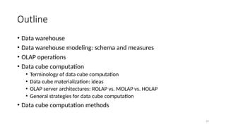
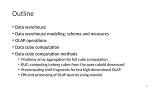
Outline
• Data warehouse
•Data warehouse modeling: schema and measures
• OLAP operations
• Data cube computation
• Data cube computation methods
3.
3
Outline
• Data warehouse
•Data warehouse: what and why?
• Architecture of data warehouses: enterprise data warehouses and data marts
• Data lakes
• Data warehouse modeling: schema and measures
• OLAP operations
• Data cube computation
• Data cube computation methods
4.
4
What is aData Warehouse?
• Defined in many different ways, but not rigorously
• A decision support database that is maintained separately from the
organization’s operational database
• Support information processing by providing a solid platform of consolidated,
historical data for analysis
• “A data warehouse is a subject-oriented, integrated, time-variant, and
nonvolatile collection of data in support of management’s decision-
making process.”—W. H. Inmon
• Data warehousing:
• The process of constructing and using data warehouses
5.
5
Data Warehouse—Subject-Oriented
• Organizedaround major subjects, such as customer, product, sales
• Focusing on the modeling and analysis of data for decision makers,
not on daily operations or transaction processing
• Provide a simple and concise view around particular subject issues by
excluding data that are not useful in the decision support process
6.
6
Data Warehouse—Integrated
• Constructedby integrating multiple, heterogeneous data sources
• relational databases, flat files, on-line transaction records
• Data cleaning and data integration techniques are applied.
• Ensure consistency in naming conventions, encoding structures, attribute
measures, etc. among different data sources
• Ex. Hotel price: differences on currency, tax, breakfast covered, and parking
• When data is moved to the warehouse, it is converted
7.
7
Data Warehouse—Time Variant
•The time horizon for the data warehouse is significantly longer than
that of operational systems
• Operational database: current value data
• Data warehouse data: provide information from a historical perspective (e.g.,
past 5-10 years)
• Every key structure in the data warehouse
• Contains an element of time, explicitly or implicitly
• But the key of operational data may or may not contain “time element”
8.
8
Data Warehouse—Nonvolatile
• Independence
•A physically separate store of data transformed from the operational
environment
• Static: Operational update of data does not occur in the data
warehouse environment
• Does not require transaction processing, recovery, and concurrency control
mechanisms
• Requires only two operations in data accessing:
• initial loading of data and access of data
9.
9
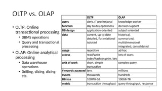
OLTP vs. OLAP
•OLTP: Online
transactional processing
• DBMS operations
• Query and transactional
processing
• OLAP: Online analytical
processing
• Data warehouse
operations
• Drilling, slicing, dicing,
etc.
10.
10
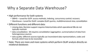
Why a SeparateData Warehouse?
• High performance for both systems
• DBMS— tuned for OLTP: access methods, indexing, concurrency control, recovery
• Warehouse—tuned for OLAP: complex OLAP queries, multidimensional view, consolidation
• Different functions and different data:
• missing data: Decision support requires historical data which operational DBs do not
typically maintain
• data consolidation: DS requires consolidation (aggregation, summarization) of data from
heterogeneous sources
• data quality: different sources typically use inconsistent data representations, codes and
formats which have to be reconciled
• Note: There are more and more systems which perform OLAP analysis directly on
relational databases
11.
11
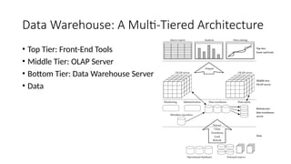
Data Warehouse: AMulti-Tiered Architecture
• Top Tier: Front-End Tools
• Middle Tier: OLAP Server
• Bottom Tier: Data Warehouse Server
• Data
12.
12
Three Data WarehouseModels
• Enterprise warehouse
• Collects all of the information about subjects spanning the entire organization
• Data Mart
• A subset of corporate-wide data that is of value to a specific groups of users
• Its scope is confined to specific, selected groups, such as marketing data mart
• Independent vs. dependent (directly from warehouse) data mart
• Virtual warehouse
• A set of views over operational databases
• Only some of the possible summary views may be materialized
13.
13
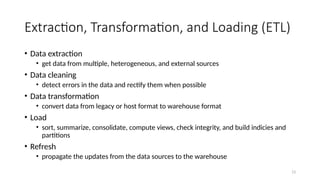
Extraction, Transformation, andLoading (ETL)
• Data extraction
• get data from multiple, heterogeneous, and external sources
• Data cleaning
• detect errors in the data and rectify them when possible
• Data transformation
• convert data from legacy or host format to warehouse format
• Load
• sort, summarize, consolidate, compute views, check integrity, and build indicies and
partitions
• Refresh
• propagate the updates from the data sources to the warehouse
14.
14
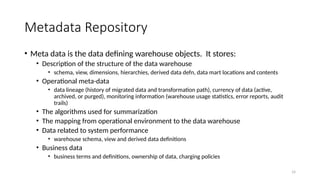
Metadata Repository
• Metadata is the data defining warehouse objects. It stores:
• Description of the structure of the data warehouse
• schema, view, dimensions, hierarchies, derived data defn, data mart locations and contents
• Operational meta-data
• data lineage (history of migrated data and transformation path), currency of data (active,
archived, or purged), monitoring information (warehouse usage statistics, error reports, audit
trails)
• The algorithms used for summarization
• The mapping from operational environment to the data warehouse
• Data related to system performance
• warehouse schema, view and derived data definitions
• Business data
• business terms and definitions, ownership of data, charging policies
15.
15
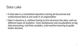
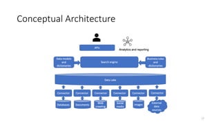
Data Lake
• Adata lake is a centralized repository storing all structured and
unstructured data at any scale in an organization
• Data is stored as is, without having to first structure the data, and run
different types of analytics—from dashboards and visualizations to big
data processing, real-time analytics, and machine learning to guide
better decision
18
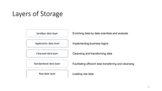
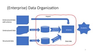
(Enterprise) Data Organization
Structureddata
Unstructured data
Unstructured data
with schema
Extraction
Parsing
Schema
Schema
inference
Schema
inference
Import
Analytics
Data lake
19.
19
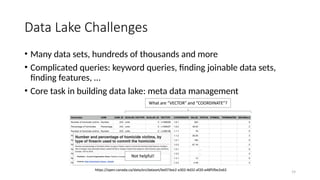
Data Lake Challenges
•Many data sets, hundreds of thousands and more
• Complicated queries: keyword queries, finding joinable data sets,
finding features, …
• Core task in building data lake: meta data management
20.
20
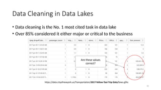
Data Cleaning inData Lakes
• Data cleaning is the No. 1 most cited task in data lake
• Over 85% considered it either major or critical to the business
21.
21
Evolving Data inData Lakes
• Many duplicates as data sets are often being copied for new projects
• Data sets are constantly being updated, having their schema altered,
being derived into new ones, and disappearing/reappearing
• Data set versioning is to maintain all versions of datasets for storage
cost-saving, collaboration, auditing, and experimental reproducibility
22.
22
Diversity in DataLakes
• Dataset formats in the open world can be highly heterogeneous
• Ingestion and extraction is the task of bringing structured datasets into
data lake
• Ingest already-structured data sets
• Extract structured data from unstructured and semi-structured data sources
• Data Integration is the task of finding joinable or union-able tables or of
on-demand population a schema with all data from the lake that
conforms to the schema
• Example: enrich Electronic Health Records (EPR) using data from various non-
standard personal health record data sets for better predicting health risks
• Joining or “union-ing” tables from different data sets and sources
24
Metadata Management inData Lakes: Ideas
• Enrich data and meta data with semantic information, support
template-based queries on metadata
• Extract deeply embedded metadata and contextual metadata to
support topic-based discovery
• Integrate metadata about data, users, and queries, and support visual
analytics
25.
25
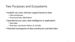
Two Purposes andEcosystems
• Analytic use cases: decision support based on data
• Data warehouses
• Structured data, SQL/Python
• Operational use cases: data intelligence in applications
• Data lakes
• Raw data, Java/Scala, Python, R, and SQL
• Potential convergence of data warehouses and data lakes
26.
26
Data Lakehouses
• “Adata lakehouse is a new, open data management architecture that
combines the flexibility, cost-efficiency, and scale of data lakes with
the data management and ACID transactions of data warehouses,
enabling business intelligence (BI) and machine learning (ML) on all
data.” (Databricks)
27.
27
Lakehouses
• Transaction support
•Schema enforcement and governance
• BI support
• Decoupling between storage and compute
• Open storage formats
• Support for diverse data types, ranging from unstructured to structured
• Support for diverse workloads: data science, machine learning, SQL and
analytics
• End-to-end streaming: real-time reports
28.
28
Data Fabric andData Virtualization
• “Data fabric is an architecture that facilitates the end-to-end
integration of various data pipelines and cloud environments through
the use of intelligent and automated systems” (IBM)
• A holistic and unified data architecture that enables organizations to
manage data across their entire ecosystem, regardless of the source,
format, location, or technology
• A data fabric provides a single point of access to all data, while
abstracting away the underlying complexity and heterogeneity of the
data landscape
29.
29
Data Mesh
• Adata mesh creates multiple domain-specific systems, each
specialized according to its functions and uses, thus bringing data
closer to consumers
• Data Mesh is a specific architecture pattern focused on data
management
30.
30
Data Virtualization
• “Datavirtualization is one of the technologies that enables a data
fabric approach. Rather than physically moving the data from various
on-premises and cloud sources using the standard ETL (extract,
transform, load) processes, a data virtualization tool connects to the
different sources, integrating only the metadata required and creating
a virtual data layer”
• Data Virtualization can be a component or a layer in a data fabric
architecture
31.
31
Outline
• Data warehouse
•Data warehouse modeling: schema and measures
• Data cube: a multidimensional data model
• Schemas for multidimensional data models: stars, snowflakes, and fact
constellations
• Concept hierarchies
• Measures: categorization and computation
• OLAP operations
• Data cube computation
• Data cube computation methods
32.
32
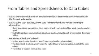
From Tables andSpreadsheets to Data Cubes
• A data warehouse is based on a multidimensional data model which views data in
the form of a data cube
• A data cube, such as sales, allows data to be modeled and viewed in multiple
dimensions
• Dimension tables, such as item (item_name, brand, type), or time(day, week, month, quarter,
year)
• Fact table contains measures (such as dollars_sold) and keys to each of the related dimension
tables
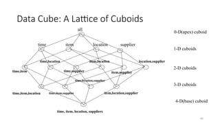
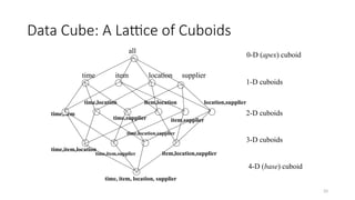
• Data cube: A lattice of cuboids
• In data warehousing literature, an n-D base cube is called a base cuboid
• The top most 0-D cuboid, which holds the highest-level of summarization, is called the apex
cuboid
• The lattice of cuboids forms a data cube.
33.
33
Data Cube: ALattice of Cuboids
time,item
time,item,location
time, item, location, supplier
all
time item location supplier
time,location
time,supplier
item,location
item,supplier
location,supplier
time,item,supplier
time,location,supplier
item,location,supplier
0-D (apex) cuboid
1-D cuboids
2-D cuboids
3-D cuboids
4-D (base) cuboid
34.
34
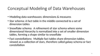
Conceptual Modeling ofData Warehouses
• Modeling data warehouses: dimensions & measures
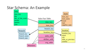
• Star schema: A fact table in the middle connected to a set of
dimension tables
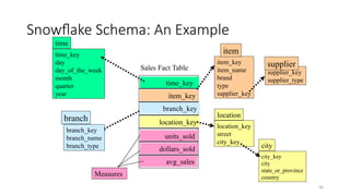
• Snowflake schema: A refinement of star schema where some
dimensional hierarchy is normalized into a set of smaller dimension
tables, forming a shape similar to snowflake
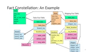
• Fact constellations: Multiple fact tables share dimension tables,
viewed as a collection of stars, therefore called galaxy schema or fact
constellation
35.
35
Star Schema: AnExample
time_key
day
day_of_the_week
month
quarter
year
time
location_key
street
city
state_or_province
country
location
Sales Fact Table
time_key
item_key
branch_key
location_key
units_sold
dollars_sold
avg_sales
Measures
item_key
item_name
brand
type
supplier_type
item
branch_key
branch_name
branch_type
branch
36.
36
Snowflake Schema: AnExample
time_key
day
day_of_the_week
month
quarter
year
time
location_key
street
city_key
location
Sales Fact Table
time_key
item_key
branch_key
location_key
units_sold
dollars_sold
avg_sales
Measures
item_key
item_name
brand
type
supplier_key
item
branch_key
branch_name
branch_type
branch
supplier_key
supplier_type
supplier
city_key
city
state_or_province
country
city
37.
37
Fact Constellation: AnExample
time_key
day
day_of_the_week
month
quarter
year
time
location_key
street
city
province_or_state
country
location
Sales Fact Table
time_key
item_key
branch_key
location_key
units_sold
dollars_sold
avg_sales
Measures
item_key
item_name
brand
type
supplier_type
item
branch_key
branch_name
branch_type
branch
Shipping Fact Table
time_key
item_key
shipper_key
from_location
to_location
dollars_cost
units_shipped
shipper_key
shipper_name
location_key
shipper_type
shipper
38.
38
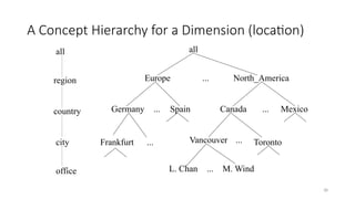
A Concept Hierarchyfor a Dimension (location)
all
Europe North_America
Mexico
Canada
Spain
Germany
Vancouver
M. Wind
L. Chan
...
...
...
... ...
...
all
region
office
country
Toronto
Frankfurt
city
39.
39
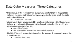
Data Cube Measures:Three Categories
• Distributive: if the result derived by applying the function to n aggregate
values is the same as that derived by applying the function on all the data
without partitioning
• E.g., count(), sum(), min(), max()
• Algebraic: if it can be computed by an algebraic function with M arguments
(where M is a bounded integer), each of which is obtained by applying a
distributive aggregate function
• avg(x) = sum(x) / count(x)
• Is min_N() an algebraic measure? How about standard_deviation()?
• Holistic: if there is no constant bound on the storage size needed to describe
a subaggregate.
• E.g., median(), mode(), rank()
40.
40
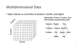
Multidimensional Data
• Salesvolume as a function of product, month, and region
Product
R
e
g
i
o
n
Month
Dimensions: Product, Location, Time
Hierarchical summarization paths
Industry Region Year
Category Country Quarter
Product City Month Week
Office Day
41.
41
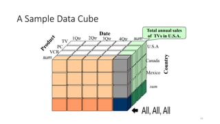
A Sample DataCube
Total annual sales
of TVs in U.S.A.
Date
P
r
o
d
u
c
t
Country
sum
sum
TV
VCR
PC
1Qtr 2Qtr 3Qtr 4Qtr
U.S.A
Canada
Mexico
sum
42.
42
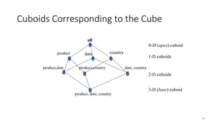
Cuboids Corresponding tothe Cube
all
product date country
product,date product,country date, country
product, date, country
0-D (apex) cuboid
1-D cuboids
2-D cuboids
3-D (base) cuboid
43.
43
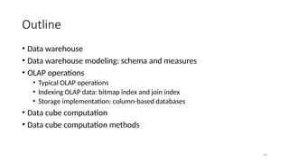
Outline
• Data warehouse
•Data warehouse modeling: schema and measures
• OLAP operations
• Typical OLAP operations
• Indexing OLAP data: bitmap index and join index
• Storage implementation: column-based databases
• Data cube computation
• Data cube computation methods
44.
44
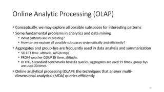
Online Analytic Processing(OLAP)
• Conceptually, we may explore all possible subspaces for interesting patterns
• Some fundamental problems in analytics and data mining
• What patterns are interesting?
• How can we explore all possible subspaces systematically and efficiently?
• Aggregates and group-bys are frequently used in data analysis and summarization
• SELECT time, altitude, AVG(temp)
• FROM weather GOUP BY time, altitude;
• In TPC, 6 standard benchmarks have 83 queries, aggregates are used 59 times, group-bys
are used 20 times
• Online analytical processing (OLAP): the techniques that answer multi-
dimensional analytical (MDA) queries efficiently
45.
45
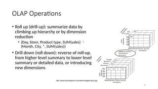
OLAP Operations
• Rollup (drill-up): summarize data by
climbing up hierarchy or by dimension
reduction
• (Day, Store, Product type, SUM(sales)
(Month, City, *, SUM(sales))
• Drill down (roll down): reverse of roll-up,
from higher level summary to lower level
summary or detailed data, or introducing
new dimensions
http://www.tutorialspoint.com/dwh/images/rollup.jpg
46.
46
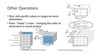
Other Operations
• Dice:pick specific values or ranges on some
dimensions
• Pivot: “rotate” a cube – changing the order of
dimensions in visual analysis
http://en.wikipedia.org/wiki/File:OLAP_pivoting.png http://www.tutorialspoint.com/dwh/images/dice.jpg
48
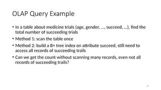
OLAP Query Example
•In a table about medicine trials (age, gender, …, succeed, …), find the
total number of succeeding trials
• Method 1: scan the table once
• Method 2: build a B+ tree index on attribute succeed, still need to
access all records of succeeding trails
• Can we get the count without scanning many records, even not all
records of succeeding trails?
49.
49
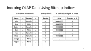
Bitmap Index
• Forn records, a bitmap index has n bits and can be packed into n
/8 bytes and n /32 words
• From a bit to the row-id: the j-th bit of the p-th byte row-id = p*8
+j
• Counting using bitmap index
• Shcount[] contains the number of bits in the entry subscript
• Example: shcount[01100101]=4
• count = 0;
• for (i = 0; i < SHNUM; i++)
• count += shcount[B[i]];
age succeed …
45 1 …
37 0 …
… … …
52 1 …
1 0 … 0
51
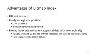
Advantages of BitmapIndex
• Efficient in space
• Ready for logic composition
• C = C1 AND C2
• Bitmap operations can be used
• Bitmap index only works for categorical data with low cardinality
• Naively, we need 50 bits per entry to represent the state of a customer in US
• How to represent a sale in dollars?
52.
52
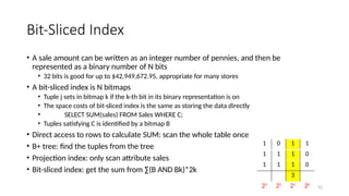
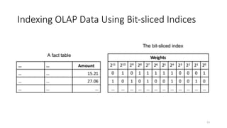
Bit-Sliced Index
• Asale amount can be written as an integer number of pennies, and then be
represented as a binary number of N bits
• 32 bits is good for up to $42,949,672.95, appropriate for many stores
• A bit-sliced index is N bitmaps
• Tuple j sets in bitmap k if the k-th bit in its binary representation is on
• The space costs of bit-sliced index is the same as storing the data directly
• SELECT SUM(sales) FROM Sales WHERE C;
• Tuples satisfying C is identified by a bitmap B
• Direct access to rows to calculate SUM: scan the whole table once
• B+ tree: find the tuples from the tree
• Projection index: only scan attribute sales
• Bit-sliced index: get the sum from ∑(B AND Bk)*2k
1 0 1 1
1 1 1 0
1 1 1 0
3
23
22
21
20
54
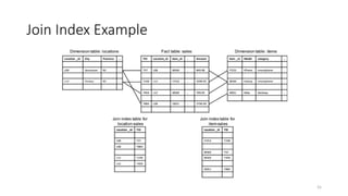
Indexing OLAP Data:Join Indices
• Join index: JI(R-id, S-id) where R (R-id, …) S (S-id, …)
• Traditional indices map the values to a list of record ids
• It materializes relational join in JI file and speeds up relational join
• In data warehouses, join index relates the values of the dimensions of
a start schema to rows in the fact table.
• E.g., fact table: Sales and two dimensions city and product
• A join index on city maintains for each distinct city a list of R-IDs of the tuples recording
the Sales in the city
• Join indices can span multiple dimensions
56
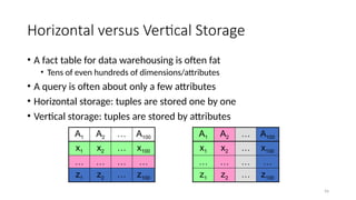
Horizontal versus VerticalStorage
• A fact table for data warehousing is often fat
• Tens of even hundreds of dimensions/attributes
• A query is often about only a few attributes
• Horizontal storage: tuples are stored one by one
• Vertical storage: tuples are stored by attributes
A1 A2 … A100
x1 x2 … x100
… … … …
z1 z2 … z100
A1 A2 … A100
x1 x2 … x100
… … … …
z1 z2 … z100
58
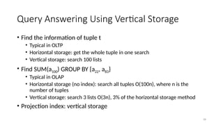
Query Answering UsingVertical Storage
• Find the information of tuple t
• Typical in OLTP
• Horizontal storage: get the whole tuple in one search
• Vertical storage: search 100 lists
• Find SUM(a100) GROUP BY {a22, a83}
• Typical in OLAP
• Horizontal storage (no index): search all tuples O(100n), where n is the
number of tuples
• Vertical storage: search 3 lists O(3n), 3% of the horizontal storage method
• Projection index: vertical storage
59.
59
Outline
• Data warehouse
•Data warehouse modeling: schema and measures
• OLAP operations
• Data cube computation
• Terminology of data cube computation
• Data cube materialization: ideas
• OLAP server architectures: ROLAP vs. MOLAP vs. HOLAP
• General strategies for data cube computation
• Data cube computation methods
60.
60
Data Cube: ALattice of Cuboids
time,item
time,item,location
time, item, location, supplierc
all
time item location supplier
time,location
time,supplier
item,location
item,supplier
location,supplier
time,item,supplier
time,location,supplier
item,location,supplier
0-D(apex) cuboid
1-D cuboids
2-D cuboids
3-D cuboids
4-D(base) cuboid
61.
61
Data Cube: ALattice of Cuboids
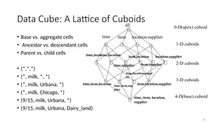
• Base vs. aggregate cells
• Ancestor vs. descendant cells
• Parent vs. child cells
• (*,*,*)
• (*, milk, *, *)
• (*, milk, Urbana, *)
• (*, milk, Chicago, *)
• (9/15, milk, Urbana, *)
• (9/15, milk, Urbana, Dairy_land)
all
time,item
time,item,location
time, item, location,
supplier
time item location supplier
time,location
time,supplier
item,location
item,supplier
location,supplier
time,item,sup
plier
time,location,suppl
ier
item,location,supplier
0-D(apex) cuboid
1-D cuboids
2-D cuboids
3-D cuboids
4-D(base) cuboid
62.
62
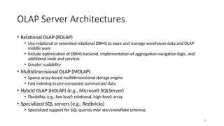
OLAP Server Architectures
•Relational OLAP (ROLAP)
• Use relational or extended-relational DBMS to store and manage warehouse data and OLAP
middle ware
• Include optimization of DBMS backend, implementation of aggregation navigation logic, and
additional tools and services
• Greater scalability
• Multidimensional OLAP (MOLAP)
• Sparse array-based multidimensional storage engine
• Fast indexing to pre-computed summarized data
• Hybrid OLAP (HOLAP) (e.g., Microsoft SQLServer)
• Flexibility, e.g., low level: relational, high-level: array
• Specialized SQL servers (e.g., Redbricks)
• Specialized support for SQL queries over star/snowflake schemas
63.
63
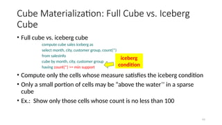
Cube Materialization: FullCube vs. Iceberg
Cube
• Full cube vs. iceberg cube
compute cube sales iceberg as
select month, city, customer group, count(*)
from salesInfo
cube by month, city, customer group
having count(*) >= min support
• Compute only the cells whose measure satisfies the iceberg condition
• Only a small portion of cells may be “above the water’’ in a sparse
cube
• Ex.: Show only those cells whose count is no less than 100
iceberg
condition
64.
64
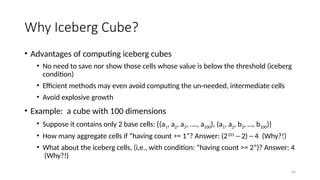
Why Iceberg Cube?
•Advantages of computing iceberg cubes
• No need to save nor show those cells whose value is below the threshold (iceberg
condition)
• Efficient methods may even avoid computing the un-needed, intermediate cells
• Avoid explosive growth
• Example: a cube with 100 dimensions
• Suppose it contains only 2 base cells: {(a1, a2, a3, …., a100), (a1, a2, b3, …, b100)}
• How many aggregate cells if “having count >= 1”? Answer: (2101
─ 2) ─ 4 (Why?!)
• What about the iceberg cells, (i,e., with condition: “having count >= 2”)? Answer: 4
(Why?!)
65.
65
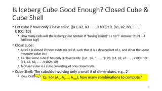
Is Iceberg CubeGood Enough? Closed Cube &
Cube Shell
• Let cube P have only 2 base cells: {(a1, a2, a3 . . . , a100):10, (a1, a2, b3, . . . ,
b100):10}
• How many cells will the iceberg cube contain if “having count(*) ≥ 10”? Answer: 2101 ─ 4
(still too big!)
• Close cube:
• A cell c is closed if there exists no cell d, such that d is a descendant of c, and d has the same
measure value as c
• Ex. The same cube P has only 3 closed cells: {(a1, a2, *, …, *): 20, (a1, a2, a3 . . . , a100): 10,
(a1, a2, b3, . . . , b100): 10}
• A closed cube is a cube consisting of only closed cells
• Cube Shell: The cuboids involving only a small # of dimensions, e.g., 2
• Idea: Only compute cube shells, other dimension combinations can be computed on the fly
Q: For (A1, A2, … A100), how many combinations to compute?
66.
66
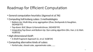
Roadmap for EfficientComputation
• General computation heuristics (Agarwal et al.’96)
• Computing full/iceberg cubes: 3 methodologies
• Bottom-Up: Multi-Way array aggregation (Zhao, Deshpande & Naughton,
SIGMOD’97)
• Top-down: BUC (Beyer & Ramarkrishnan, SIGMOD’99)
• Integrating Top-Down and Bottom-Up: Star-cubing algorithm (Xin, Han, Li & Wah:
VLDB’03)
• High-dimensional OLAP:
• A Shell-Fragment Approach (Li, et al. VLDB’04)
• Computing alternative kinds of cubes:
• Partial cube, closed cube, approximate cube, ……
67.
67
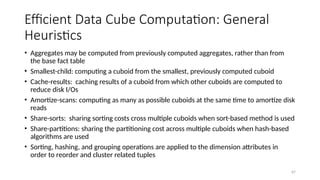
Efficient Data CubeComputation: General
Heuristics
• Aggregates may be computed from previously computed aggregates, rather than from
the base fact table
• Smallest-child: computing a cuboid from the smallest, previously computed cuboid
• Cache-results: caching results of a cuboid from which other cuboids are computed to
reduce disk I/Os
• Amortize-scans: computing as many as possible cuboids at the same time to amortize disk
reads
• Share-sorts: sharing sorting costs cross multiple cuboids when sort-based method is used
• Share-partitions: sharing the partitioning cost across multiple cuboids when hash-based
algorithms are used
• Sorting, hashing, and grouping operations are applied to the dimension attributes in
order to reorder and cluster related tuples
68.
68
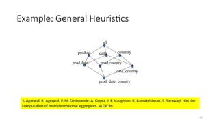
Example: General Heuristics
S.Agarwal, R. Agrawal, P. M. Deshpande, A. Gupta, J. F. Naughton, R. Ramakrishnan, S. Sarawagi. On the
computation of multidimensional aggregates. VLDB’96
all
product date country
prod,date prod,country
date, country
prod, date, country
69.
69
Outline
• Data warehouse
•Data warehouse modeling: schema and measures
• OLAP operations
• Data cube computation
• Data cube computation methods
• Multiway array aggregation for full cube computation
• BUC: computing iceberg cubes from the apex cuboid downward
• Precomputing shell fragments for fast high-dimensional OLAP
• Efficient processing of OLAP queries using cuboids
70.
70
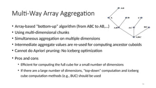
Multi-Way Array Aggregation
•Array-based “bottom-up” algorithm (from ABC to AB,…)
• Using multi-dimensional chunks
• Simultaneous aggregation on multiple dimensions
• Intermediate aggregate values are re-used for computing ancestor cuboids
• Cannot do Apriori pruning: No iceberg optimization
• Pros and cons
• Efficient for computing the full cube for a small number of dimensions
• If there are a large number of dimensions, “top-down” computation and iceberg
cube computation methods (e.g., BUC) should be used
ABC
AB
A
All
B
AC BC
C
71.
71
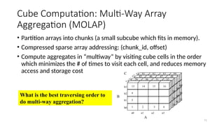
Cube Computation: Multi-WayArray
Aggregation (MOLAP)
• Partition arrays into chunks (a small subcube which fits in memory).
• Compressed sparse array addressing: (chunk_id, offset)
• Compute aggregates in “multiway” by visiting cube cells in the order
which minimizes the # of times to visit each cell, and reduces memory
access and storage cost
What is the best traversing order to
do multi-way aggregation?
A
B
29 30 31 32
1 2 3 4
5
9
13 14 15 16
64
63
62
61
48
47
46
45
a1
a0
c3
c2
c1
c 0
b3
b2
b1
b0
a2 a3
C
B
44
28
56
40
24
52
36
20
60
72.
72
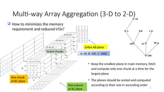
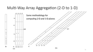
Multi-way Array Aggregation(3-D to 2-D)
all
A B
A B
A BC
A C BC
C
• Keep the smallest plane in main memory, fetch
and compute only one chunk at a time for the
largest plane
• The planes should be sorted and computed
according to their size in ascending order
ABC
AB
A
All
B
AC BC
C
How to minimizes the memory
requirement and reduced I/Os?
Entire AB plane
One column
of AC plane
One chunk
of BC plane
4x4x4 chunks
A: 40, B: 400, C: 4000
74
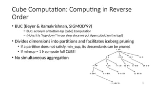
Cube Computation: Computingin Reverse
Order
• BUC (Beyer & Ramakrishnan, SIGMOD’99)
• BUC: acronym of Bottom-Up (cube) Computation
• (Note: It is “top-down” in our view since we put Apex cuboid on the top!)
• Divides dimensions into partitions and facilitates iceberg pruning
• If a partition does not satisfy min_sup, its descendants can be pruned
• If minsup = 1 Þ compute full CUBE!
• No simultaneous aggregation
1 a ll
2 A 1 0 B 1 4 C
7 A C 1 1 B C
4 A B C 6 A B D 8 A C D 1 2 B C D
9 A D 1 3 B D 1 5 C D
1 6 D
5 A B C D
3 A B
75.
75
BUC: Partitioning andAggregating
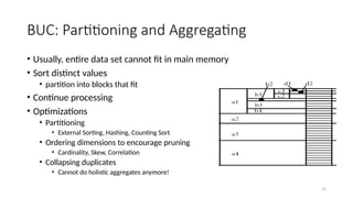
• Usually, entire data set cannot fit in main memory
• Sort distinct values
• partition into blocks that fit
• Continue processing
• Optimizations
• Partitioning
• External Sorting, Hashing, Counting Sort
• Ordering dimensions to encourage pruning
• Cardinality, Skew, Correlation
• Collapsing duplicates
• Cannot do holistic aggregates anymore!
76.
76
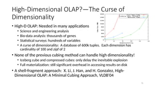
• High-D OLAP:Needed in many applications
• Science and engineering analysis
• Bio-data analysis: thousands of genes
• Statistical surveys: hundreds of variables
• A curse of dimensionality: A database of 600k tuples. Each dimension has
cardinality of 100 and zipf of 2
• None of the previous cubing method can handle high dimensionality!
• Iceberg cube and compressed cubes: only delay the inevitable explosion
• Full materialization: still significant overhead in accessing results on disk
• A shell-fragment approach: X. Li, J. Han, and H. Gonzalez, High-
Dimensional OLAP: A Minimal Cubing Approach, VLDB'04
High-Dimensional OLAP?—The Curse of
Dimensionality
77.
77
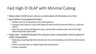
Fast High-D OLAPwith Minimal Cubing
• Observation: OLAP occurs only on a small subset of dimensions at a time
• Semi-Online Computational Model
• Partition the set of dimensions into shell fragments
• Compute data cubes for each shell fragment while retaining inverted indices or value-list
indices
• Given the pre-computed fragment cubes, dynamically compute cube cells of the high-
dimensional data cube online
• Major idea: Tradeoff between the amount of pre-computation and the speed of
online computation
• Reducing computing high-dimensional cube into precomputing a set of lower dimensional
cubes
• Online re-construction of original high-dimensional space
• Lossless reduction
78.
78
Computing a 5-DCube with 2-Shell Fragments
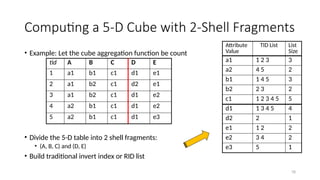
• Example: Let the cube aggregation function be count
• Divide the 5-D table into 2 shell fragments:
• (A, B, C) and (D, E)
• Build traditional invert index or RID list
tid A B C D E
1 a1 b1 c1 d1 e1
2 a1 b2 c1 d2 e1
3 a1 b2 c1 d1 e2
4 a2 b1 c1 d1 e2
5 a2 b1 c1 d1 e3
Attribute
Value
TID List List
Size
a1 1 2 3 3
a2 4 5 2
b1 1 4 5 3
b2 2 3 2
c1 1 2 3 4 5 5
d1 1 3 4 5 4
d2 2 1
e1 1 2 2
e2 3 4 2
e3 5 1
79.
79
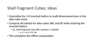
Shell Fragment Cubes:Ideas
• Generalize the 1-D inverted indices to multi-dimensional ones in the
data cube sense
• Compute all cuboids for data cubes ABC and DE while retaining the
inverted indices
• Ex. shell fragment cube ABC contains 7 cuboids:
• A, B, C; AB, AC, BC; ABC
• This completes the offline computation
80.
80
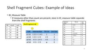
• ID_Measure Table
•If measures other than count are present, store in ID_measure table separate
from the shell fragments
Shell Fragment Cubes: Example of Ideas
Attribute
Value
TID List List
Size
a1 1 2 3 3
a2 4 5 2
b1 1 4 5 3
b2 2 3 2
c1 1 2 3 4 5 5
d1 1 3 4 5 4
d2 2 1
e1 1 2 2
e2 3 4 2
e3 5 1
Cell Intersection TID List List Size
a1 b1 1 2 3 ∩ 1 4 5 1 1
a1 b2 1 2 3 ∩ 2 3 2 3 2
a2 b1 4 5 ∩ 1 4 5 4 5 2
a2 b2 4 5 ∩ 2 3 φ 0
tid count sum
1 5 70
2 3 10
3 8 20
4 5 40
5 2 30
Shell-fragment AB
81.
81
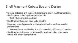
Shell Fragment Cubes:Size and Design
• Given a database of T tuples, D dimensions, and F shell fragment size,
the fragment cubes’ space requirement is
• For F < 5, the growth is sub-linear
• Shell fragments do not have to be disjoint
• Fragment groupings can be arbitrary to allow for maximum online
performance
• Known common combinations (e.g.,<city, state>) should be grouped together
• Shell fragment sizes can be adjusted for optimal balance between
offline and online computation
82.
82
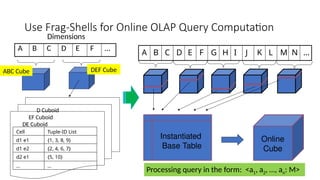
Use Frag-Shells forOnline OLAP Query Computation
A B C D E F …
ABC Cube DEF Cube
D Cuboid
EF Cuboid
DE Cuboid
Cell Tuple-ID List
d1 e1 {1, 3, 8, 9}
d1 e2 {2, 4, 6, 7}
d2 e1 {5, 10}
… …
Dimensions
A B C D E F G H I J K L M N …
Online
Cube
Instantiated
Base Table
Processing query in the form: <a1, a2, …, an: M>
83.
83
Online Query Computationwith Shell-
Fragments
• A query has the general form: <a1, a2, …, an: M>
• Each ai has 3 possible values (e.g., <3, ?, ?, *, 1: count> returns a 2-D data
cube)
• Instantiated value
• Aggregate * function
• Inquire ? Function
• Method: Given the materialized fragment cubes, process a query as follows
• Divide the query into fragments, same as the shell-fragment
• Fetch the corresponding TID list for each fragment from the fragment cube
• Intersect the TID lists from each fragment to construct instantiated base table
• Compute the data cube using the base table with any cubing algorithm
Editor's Notes
#13 MK 08.11.09 Former title: Data Warehouse Back-End Tools and Utilities
#63 2*(2^{100}-1)-1, 1
Explanation: one cell, such as (a1, a2, …., a100) generates 2^100 -1 aggregate cells, because choose(100 1) + choose (100 2) + ... choose (100, 100) = 2^100 - 1 aggregate cells.
For two cell question, it generates 2 * (2^100-1) -1 distinct aggregate cells because (*, *, …, *) generated by (a1, a2, …., a100) and (b1, b2, …, b100) will be merged into one cell:
(*, *, …, *): 2. Hence we have 2*(2^{100}-1)-1
#64 For {(a1, a2, a3 . . . , a100), (a1, a2, b3, . . . , b100)}, the total # of non-base cells should be 2 * (2^{100} – 1) – 4.
This is calculated as follows:
(a1, a2, a3 . . . , a100) will generate 2^{100} - 1 non-base cells
(a1, a2, b3, . . . , b100) will generate 2^{100} - 1 non-base cells
Among these, 4 cells are overlapped and thus minus 4 so we get: 2*2^{100} - 2 - 4 = 2*2^{100} - 6
These 4 cells are:
(a1, a2, *, ..., *): 2
(a1, *, *, ..., *): 2
(*, a2, *, ..., *): 2
(*, *, *, ..., *): 2


![49
Bitmap Index
• For n records, a bitmap index has n bits and can be packed into n
/8 bytes and n /32 words
• From a bit to the row-id: the j-th bit of the p-th byte row-id = p*8
+j
• Counting using bitmap index
• Shcount[] contains the number of bits in the entry subscript
• Example: shcount[01100101]=4
• count = 0;
• for (i = 0; i < SHNUM; i++)
• count += shcount[B[i]];
age succeed …
45 1 …
37 0 …
… … …
52 1 …
1 0 … 0](https://image.slidesharecdn.com/chap3-datawarehousingandolap-250321040420-72c587b8/85/Chap3-Data-Warehousing-and-OLAP-operations-pptx-49-320.jpg)