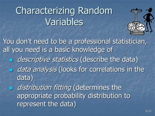
2. 5-2
Questions to be answered:
What types of data should be gathered?
How should data be gathered?
What statistical background do I need?
How should data be analyzed?
How do you get data in the right form for
use in simulation?
How should data be documented?
3. 5-3
Objective of Data Collection and
Analysis
The goal of data collection and analysis it to
come up with descriptive information and
statistics that define the behavior of the
system.
4. 5-4
What Types of Data Should Be
Gathered?
Structural
Operational
Numerical
7. 5-7
Numerical Data
Resource quantities
Buffer sizes
Operation times
Move times
Interarrival times
Batch sizes
Time between failures
Requires
some
statistical
analysis
8. 5-8
How Should Data Be Gathered?
1. Determine data requirements.
2. Identify reliable data sources.
3. Collect the data.
4. Summarize the data
5. Document and approve data.
9. 5-9
Suggestions for Data Gathering
Define the problem/objective for the simulation
(maximize throughput, minimize cycle time, etc.)
Identify only factors that bear on the problem
(operation times, resource scheduling, etc.)
Focus on input variables, not response variables (flow
times, throughput rates, utilizations, etc.)
Separate delay times from delay conditions (e.g. getting
a resource vs. activity time).
Look for common groupings (e.g., part families)
Focus on essence (i.e. time, conditions), not substance
(i.e. how the activity is performed).
Look for triggering events (What triggers entity
movement? What triggers a machine setup?).
10. 5-10
Look for the Constraints
A system constraint is anything that keeps
everything from happening all at once.
Constraints include time delays,
conditional delays due to unavailable
resources, parts, etc.
11. 5-11
Use a Questionnaire
Organizes and simplifies the data
gathering process.
Helps ensure all issues are addressed.
Can send it to process owners in
advance and leave a copy afterwards
12. 5-12
Sources of Data
Historical records (production, sales,
scrap rates, equipment reliability)
System documentation (process plans,
facility layouts, work procedures)
Personal Observation (facility walk-
through, time studies, work sampling)
Interviews (operators, maintenance
personnel, engineers, managers)
13. 5-13
Sources of Data (cont.)
Comparative systems (same or similar
industries)
Vendor claims (cycle times, equipment
reliability)
Design estimates (process times, move
times, etc. for a new system)
Literature (published research on
learning curves, predetermined time
studies, etc.)
14. 5-14
What to Avoid
Opinions when actual times can be
determined.
Taking only one or two sample times.
Taking samples from only one day or only
one operator then applying the results to
many operators.
20. 5-20
Random System Variables
Qualitative variable -- A non-numerically valued variable.
Quantitative variable -- A numerically valued variable.
Discrete Variable -- A quantitative variable whose possible
values form a finite set of specific values (categories for
qualitative data, whole numbers for quantitative data).
Continuous variable -- A quantitative variable whose
possible values can vary infinitely within a range.
Defining characteristics of a system that vary in value from
one observation to the next (e.g. cycle time, boxes per
pallet).
21. 5-21
Characterizing Random
Variables
descriptive statistics (describe the data)
data analysis (looks for correlations in the
data)
distribution fitting (determines the
appropriate probability distribution to
represent the data)
You don’t need to be a professional statistician,
all you need is a basic knowledge of
22. 5-22
Discrete vs. Continuous Variables
Continuous – The variable can take on
any value within a range (i.e. Height,
Weight, Time, etc.)
Discrete – The variable can only take
select values within a range (i.e. Gender,
Patient Class, Part Type, Counts, etc.)
23. 5-23
Data for a Variable
A random system variable is defined by
gathering sample data on the variable.
For random variables, the more data that
are gathered (i.e., the larger the sample
size), the more accurate the
characterization is of the variable.
24. 5-24
Data Groupings
Class – Category or range of values for
grouping data.
Frequency -- The number of observations that
fall in a class.
Frequency distribution -- A listing of all
classes along with their frequencies.
Relative frequency -- The ratio of the
frequency of a class to the total number of
observations.
Relative-frequency distribution -- A listing
of all classes along with their relative
frequencies.
25. 5-25
Histograms vs. Bar Charts
•Used for quantitative variables
•Horizontal axis shows range
•Bars touch each other
•Used for categorical variables
•Horizontal axis shows category
•Bars don’t touch each other
26. 5-26
Age Tally Frequency Relative
Frequency
Percent
25 to < 33 |||| 5 5/50 = .10 10%
33 to < 41 |||| |||| |||| 14 14/50 = .28 28%
41 to < 49 |||| |||| ||| 13 13/50 = .26 26%
49 to < 57 |||| |||| 9 9/50 = .18 18%
57 to < 65 |||| || 7 7/50 = .14 14%
65 to < 73 || 2 2/50 = .04 4%
A Histogram is used
to show frequency or
percentage by
interval (data will
always be numerical)
28. 5-28
Histograms reveal the shape,
center, and spread of a variable
Shape refers to the shape formed by
the bars of the histogram
Center refers to the mean of the
variable. If the histogram were an
object, it would “balance” on the mean
(half the area is to the left, half to the
right).
Spread refers to how far dispersed the
data values are
30. 5-30
Calculating Sample Mean
n
i
X
X
Formula:
That is, add up all of the data points and divide
by the number of data points.
Data (# of classes skipped): 2 8 3 4 1
Sample Mean = (2+8+3+4+1)/5 = 3.6
Do not round! Mean need not be a whole number.
31. 5-31
Median
Another name for 50th percentile.
Appropriate for describing measurement
data.
“Robust to outliers,” that is, not
affected much by unusual values.
32. 5-32
Mode
The value that occurs most frequently.
One data set can have many modes.
Appropriate for all types of data, but most
useful for categorical data or discrete data
with only a few number of possible values.
36. 5-36
How and why should data be
analyzed?
Data analysis ensures that your data is
meaningful and useful.
Types of analysis include:
Test for independence (randomness).
Test for homogeneity (same source).
Test for stationarity (non varying over time).
37. 5-37
Testing for Independence
(Randomness)
Scatter Plot
Autocorrelation Plot
Runs Test
These tests can be run using Stat::Fit
which can be run “Stand-alone” or from
the ProModel Tools menu.
38. 5-38
Stat::Fit
Stat::Fit is the data analysis and
distribution fitting software package
bundled with PROMODEL products.
You can enter or import a dataset into
Stat::Fit for distribution fitting.
You can copy and paste the fitted
distribution parameters into a ProModel
model.
39. 5-39
Entering Data in Stat::Fit
Type values.
Open a .dat file
(File Open).
Copy and paste
from spreadsheet.
40. 5-40
Scatter Plot
Tests for Independence.
Plots successive pairs of data as x,y values
(n-1 points).
Random scatter of points indicates
independence.
If data are correlated, the points will fall
along a line or curve.
43. 5-43
Autocorrelation Plot
Another test for independence.
Independence is ascertained by computing
autocorrelations for data values at varying
time lags.
If independent, such autocorrelations
should be near zero for any and all time-
lag separations.
46. 5-46
Data that tends to be non-
homogenous
Activity times that take longer or
shorter depending on the type of entity
being processed.
Inter-arrival times that fluctuate in
length depending on the time of day or
day of the week.
Time between failures and time to
repair where the failure may result from
a number of different causes.
47. 5-47
Testing for Identically Distributed
(Homogenous) Data
Repair Time
Frequency
of
Occurrence
Part Jams Mechanical Failures
Bimodal Distribution of Downtimes Indicating Multiple Causes
49. 5-49
Non-stationary Data
Time of Day
Rate of
Arrival
10:00 a.m. 12:00 a.m. a.m. 2:00 p.m. 4:00 p.m. 6:00 p.m.
Change in Rate of Customer Arrivals Between 10 a.m. and 6 p.m.
50. 5-50
Three ways to represent data
Use actual data -- e.g. read from text file
Use a frequency table -- called an
empirical or user-defined distribution
Use a standard distribution -- best guess
or Stat::Fit
51. 5-51
Probability Distributions
A Probability Distribution defines all
possible values of a system variable
plotted against their respective
probabilities.
Distributions can be either discrete
(probability mass function) or continuous
(probability density function).
52. 5-52
Bernoulli
The output of a process is either defective
or non-defective
An employee shows up for work or not
An operation is required or not
f(x)
x
0 1
1.0
0.5
53. 5-53
Binomial
The number of defective items in a batch.
The number of customers of a particular
type that enter the system.
The number of employees out of a group
of employees who call in sick on a given
day.
f(x)
x
0 1 2 3 4 5 6
.4
.3
.2
.1
54. 5-54
The number of entities arriving each hour.
The number of defects per item.
The number of times a resource is
interrupted each hour.
Poisson
f(x)
x
0.2
0.1
0 1 2 3 4 5 6 7 8 9 10
55. 5-55
The number of machine cycles before a
failure occurs.
The number of items inspected before a
defective item is found.
The number of customers processed
before a particular type is encountered
Geometric
f(x)
x
1 2 3 4 5 6 7
0
0.4
0.3
0.2
0.1
56. 5-56
The type of an incoming entity given that
each possible type is equally likely to
occur
Uniform
f(x)
x
a b
57. 5-57
f(x)
x
a m c
Triangular
• good first approximation to the true
underlying distribution when data is sparse
and no distribution fitting analysis has been
performed
58. 5-58
Popular but rarely a true representation of
actual data.
Normal
f(x)
x
59. 5-59
intervals between occurrences such as
the time between customer arrivals.
certain repair times or activities such as
the duration of telephone conversations.
Inverse of Poisson
Exponential
f(x)
x
60. 5-60
random proportions such as the
percentage of defective items in a lot
activity times, particularly when multiple
tasks make up the activity (PERT
analysis is based on beta distribution).
Beta
f(x)
x
=0.5, =2
=1.0, =2.0
=.5, =.5
1.0
0
61. 5-61
manual activities such as assembly,
inspection or repair.
The time between failures is often
lognormally distributed.
Lognormal
f(x)
x
62. 5-62
manual tasks such as service times or
repair times
Gamma
f(x)
x
>
1
2
63. 5-63
used in reliability theory for defining the
time until failure particularly due to
items (e.g. bearings, tooling, etc.) that
wear
Weibull
f(x)
x
=
1
2
64. 5-64
Bounded vs. Boundless
Distributions
Bounded distributions prevent likely
extreme values from occurring.
Boundless distributions cause unlikely
extreme values to occur.
65. 5-65
Fitting Distributions to Data Using
Stat::Fit
1. Enter or import data as previously
discussed.
2. Plot the data and look at parameters to
get a sense of the shape of the data.
3. Select distributions to fit and analysis to
use.
4. Run the analysis and view rankings.
5. Make a selection.
66. 5-66
Plotting the Data
To plot the raw data
you have imported
select Input Input
Graph
The shape of the input
graph can help
determine the
appropriate distribution.
67. 5-67
Descriptive Statistics
If desired, you can view
descriptive statistics
(data parameters) for
the data to get an idea
of the center and
spread.
Select Statistics
Descriptive
68. 5-68
Setup
Select Fit Setup
The window that
comes up allows you
to select the
distributions Stat::Fit
will fit to the data set.
70. 5-70
Estimators
Stat::Fit allows you to
change the estimation
technique utilized to fit
the distributions.
MLE’s (Maximum
Likelihood Estimators)
are generally preferred,
but in some cases the
MLE estimator doesn’t
exist so you must use
Moments.
71. 5-71
Tests
You can choose to
perform any
combination of the
three goodness of fit
tests that are available.
All three tests measure
the extent that the fit
distribution models the
data set but in different
ways.
72. 5-72
Chi-Squared Test
1. Compares actual counts(values from the
input dataset) versus expected counts
(values from the estimated distribution)
2. Derives p-value from how much these
values differ
3. Better with larger sample sizes
73. 5-73
Kolmogorov-Smirnov Test
1. Difference between cumulative
distribution of data and fit distribution
2. Most conservative, least likely to reject
the correct distribution in error
74. 5-74
Anderson-Darling Test
1. Like Kolmogorov Smirnov, but gives a
heavier weight to differences in the tails of
the distribution
2. Good for any sample size
3. Not good for discrete data
75. 5-75
Tests
The Hypotheses:
H0: The distribution fit is in fact the correct
distribution to describe the variable of
interest.
H1: The distribution fit is NOT the correct
distribution to describe the variable of
interest.
76. 5-76
How often are you willing to be
wrong?
You set the value of the
level of significance
based on the answer
to the question
above.
Tells you how likely the
test rejects a
distribution that
accurately describes
the data.
77. 5-77
Errors
There are two types of errors that can be
made when performing a statistical test:
Type I: you reject H0 when in fact H0 is true
Type II: you accept H0 when if fact H1 is true
The level of significance you chose IS the
probability of a Type I error
78. 5-78
Fitting the Data
There are two ways to perform the goodness
of fit tests:
Select the Auto::Fit button from the toolbar
Select Fit Goodness of Fit
79. 5-79
Auto::Fit
Within the Auto::Fit
window you can select
to fit continuous or
discrete distributions.
If the distribution has a
lower bound, that value
can be specified here.
81. 5-81
Goodness of Fit Tests
The test results are given
along with the actual
distribution fit. Each test
has a result: Reject or Do
Not Reject.
Do Not Reject means
there was not enough
evidence to conclude it is
not the correct
distribution to describe
the data.
82. 5-82
Distribution Graph
After picking out the top
few distributions, it can
be useful to graph the
fit distribution against
the data.
Select Fit Results
Graph Comparison
83. 5-83
Picking a Fit
Compare test results.
Compare graphs.
Use what you know about the
process.
84. 5-84
Exporting
Once you have selected
a fit, you need to export
it to the PROMODEL
product.
Select File Export
Export Fit or the
Export button from the
toolbar.
85. 5-85
Exporting
Select the application
you would like to
export to (PROMODEL
Products)
Select the distribution
to export
86. 5-86
Exporting
The precision box
allows you to change
the number of
decimal places in the
distribution
parameters
Select OK
The distribution is
now in the correct
form to paste into
your model
87. 5-87
Stat::Fit
What to avoid:
Small samples
Using all goodness of fit tests – it
increases the Type I error rate
Taking the distribution into the
model without exporting
91. 5-91
Appropriate Adjustments
Remember, you fit a distribution to
historical data, not necessarily to the
data reflecting the design period.
Don’t forget to adjust the data to reflect
the period of interest.
Is there a growth rate to factor in?
Is there a learning curve to consider?
92. 5-92
Handling Rare Behavior
Repeating behavior – e.g. Occasional
abnormally long downtimes.
Can include if not too infrequent.
Can model once like non-repeating.
Non-repeating behavior – e.g. Labor strike
Throw one in to see what happens.
93. 5-93
Absence of Data
A single, most likely or mean value
Minimum and maximum values defining a range
Minimum, most likely and maximum values
Use sensitivity analysis:
Best case
Worse case
Most likely case
94. 5-94
Assumptions
All models are based on assumptions.
Relative comparisons may still be valid.
Sensitivity analysis can show crucial
assumptions.
95. 5-95
Data Documentation and
Approval
Tables
Flow Diagrams
Assumption Lists
Exclusion Lists
Sources Used
Consent (not necessarily validation)
from users and decision makers
96. 5-96
Use of Flowchart
Station 1
Station 3
19”, 21” & 25”
Monitors
Station 2 Inspection
Rejected Monitors
25” Monitor
19” & 21” Monitor
Reworked
Monitors
97. 5-97
Use of Tables
Entity Station Opn. Time (min, mode, max)
19" Monitor Station 1 .8, 1, 1.5
Station 2 .9, 1.2, 1.8
Inspection 1.8, 2.2, 3
21” Monitor Station 1 .8, 1, 1.5
Station 2 1.1, 1.3, 1.9
Inspection 1.8, 2.2, 3
25” Monitor Station 1 .9, 1.1, 1.6
Station 2 1.2, 1.4, 2
Inspection 1.8, 2.3, 3.2
Station 3 .5, .7, 1
98. 5-98
Use of Operation Rules
l Defective monitors are detected at inspection and routed to
whichever station created the problem.
l Monitors waiting at a station for rework have a higher
priority than first time monitors.
l Corrected monitors are routed back to inspection.
l A reworked monitor fails a second time it is removed from
the system.
Handling Defective Monitors
99. 5-99
Use of an Assumption List
l No downtimes are considered (downtimes are rare).
l Operators are dedicated at each workstation and are always
available during the scheduled work time.
l Rework times are half of the normal operation times.
Assumptions
100. 5-100
Remember…
Information is never accurate or sufficient enough
to make a “no risk” decision. But the better the
information, the less risky the decision.