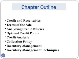
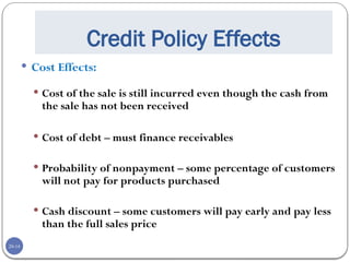
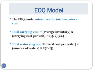
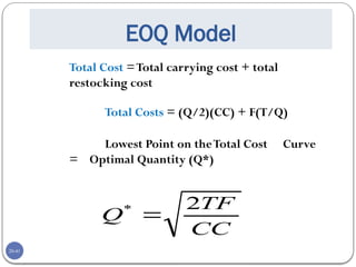
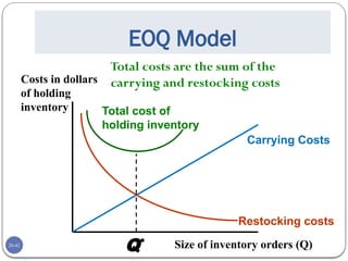
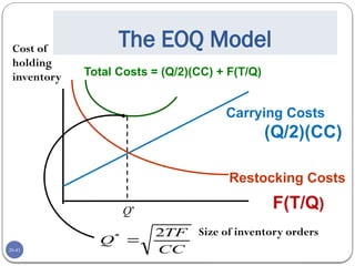
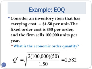
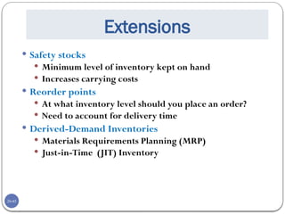
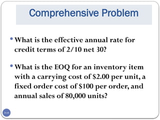
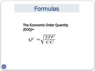
20-1
Credit and Inventory Management
Chapter
20
Copyright © 2013 by The McGraw-Hill Companies, Inc. All rights reserved.
McGraw-Hill/Irwin
20-2
Chapter Outline
• Credit and Receivables
• Terms of the Sale
• Analyzing Credit Policies
• Optimal Credit Policy
• Credit Analysis
• Collection Policy
• Inventory Management
• Inventory ManagementTechniques
20-3
Chapter Outline
(Appendix)
• Alternative Credit Policy Analysis
The One-Shot Approach
The AR Approach
• Discounts and Default model
20-4
Chapter Outline
• Credit and Receivables
• Terms of the Sale
• Analyzing Credit Policies
• Optimal Credit Policy
• Credit Analysis
• Collection Policy
• Inventory Management
• Inventory ManagementTechniques
20-5
Credit Management: Key Issues
 Granting credit generally increases sales
 Costs of granting credit
 Chance that customers
will not pay
 Financing receivables
 Credit management examines the trade-off
between increased sales and the costs of
granting credit
20-6
Components of Credit
Policies
Terms of sale
 Credit period
 Cash discount and discount period
 Type of credit instrument
Credit analysis
Distinguishing between “good”
customers that will pay and “bad”
customers that will default
20-7
Components of Credit
Policies
Collection policy
Effort expended on collecting
receivables
20-8
The Cash Flows from
Granting Credit
Credit Sale Check Mailed Check Deposited Cash
Available
Cash Collection
Accounts Receivable
20-9
Chapter Outline
• Credit and Receivables
• Terms of the Sale
• Analyzing Credit Policies
• Optimal Credit Policy
• Credit Analysis
• Collection Policy
• Inventory Management
• Inventory ManagementTechniques
20-10
Terms of Sale
Basic Form: 2/10 net 45
 2% discount if paid in 10 days
 Total amount due in 45 days if discount not taken
Buy $500 worth of merchandise with the credit terms
given above
 Pay $500(1 - .02) = $490 if you pay in 10 days
 Pay $500 if you pay in 45 days
20-11
Example: Cash Discounts
 Finding the implied interest rate when customers do not
take the discount
 Credit terms of 2/10 net 45
 Period rate = 2 / 98 = 2.0408%
 Period = (45 – 10) = 35 days
 365 / 35 = 10.4286 periods per year
 EAR = (1.020408)10.4286
– 1 = 23.45%
 The company benefits when customers choose to forgo
discounts
20-12
Chapter Outline
• Credit and Receivables
• Terms of the Sale
• Analyzing Credit Policies
• Optimal Credit Policy
• Credit Analysis
• Collection Policy
• Inventory Management
• Inventory ManagementTechniques
20-13
Credit Policy Effects
Revenue Effects:
Delay in receiving cash
from sales
May be able to increase
price
May increase total sales
20-14
Credit Policy Effects
 Cost Effects:
 Cost of the sale is still incurred even though the cash from
the sale has not been received
 Cost of debt – must finance receivables
 Probability of nonpayment – some percentage of customers
will not pay for products purchased
 Cash discount – some customers will pay early and pay less
than the full sales price
20-15
Example: Evaluating a
Proposed Policy – Part I
 Your company is evaluating a switch from a cash only
policy to a net 30 policy.The price per unit is $100, and
the variable cost per unit is $40.The company currently
sells 1,000 units per month. Under the proposed policy,
the company expects to sell 1,050 units per month.The
required monthly return is 1.5%.
 What is the NPV of the switch?
 Should the company offer credit terms of net 30?
20-16
Example: Evaluating a
Proposed Policy – Part II
 Incremental cash inflow
(100 – 40)(1,050 – 1,000) = $3,000
 Present value of incremental cash inflow
3,000/.015 = $200,000
 Cost of switching
100(1,000) + 40(1,050 – 1,000) = $102,000
 NPV of switching
200,000 – 102,000 = $98,000
 Yes, the company should switch!
20-17
Total Cost of Granting Credit
 Carrying costs
 Required return on receivables
 Losses from bad debts
 Costs of managing credit and collections
 Shortage costs
 Lost sales due to a restrictive credit policy
 Total cost curve
 Sum of carrying costs and shortage costs
 Optimal credit policy is where the total cost curve is
minimized
20-18
Chapter Outline
• Credit and Receivables
• Terms of the Sale
• Analyzing Credit Policies
• Optimal Credit Policy
• Credit Analysis
• Collection Policy
• Inventory Management
• Inventory ManagementTechniques
20-19
Carrying and Opportunity
Costs
20-20
Chapter Outline
• Credit and Receivables
• Terms of the Sale
• Analyzing Credit Policies
• Optimal Credit Policy
• Credit Analysis
• Collection Policy
• Inventory Management
• Inventory ManagementTechniques
20-21
Credit Analysis
 The process of deciding which customers receive credit
 Gathering information
 Financial statements
 Credit reports
 Banks
 Payment history with the firm
 Determining Creditworthiness
 5 Cs of Credit
 Credit Scoring
20-22
One-Time Sale Model
NPV = -v + (1 - )P / (1 + R)
where: v = variable cost per unit
 = probability of
default
P = Current Price
R = Monthly required
return
20-23
Example: One-Time Sale
Your company is considering granting
credit to a new customer.
The variable cost per unit is $50; the
current price is $110;
The probability of default is 15%;
The monthly required return is 1%.
20-24
One-Time Sale Model
NPV = -v + (1 - )P / (1 + R)
NPV = -50 + (1-.15)(110)/(1.01)
= $42.57
What is the break-even probability?
NPV = $0 = -50 + (1 - )(110)/(1.01)
 = .5409 or 54.09%
20-25
Example: Repeat Customers
In the previous example, what is the
NPV if we are looking at repeat
business?
NPV = -v + (1-)(P – v)/R
NPV = -50 + (1-.15)(110 – 50)/.01
= $5,050
20-26
Example: Repeat Customers
Interpretation
 Repeat customers can be very valuable (hence the
importance of good customer service)
 It may make sense to grant credit to almost
everyone once, as long as the variable cost is low
relative to the price
 If a customer defaults once, you don’t grant credit
again
20-27
Credit Information
Financial statements
Credit reports with customer’s
payment history to other firms
Banks
Payment history with the company
20-28
Five Cs of Credit
 Character – willingness to
meet financial obligations
 Capacity – ability to meet financial obligations out of
operating cash flows
 Capital – financial reserves
 Collateral – assets pledged as security
 Conditions – general economic conditions related to
customer’s business
CCCCC
20-29
Chapter Outline
• Credit and Receivables
• Terms of the Sale
• Analyzing Credit Policies
• Optimal Credit Policy
• Credit Analysis
• Collection Policy
• Inventory Management
• Inventory ManagementTechniques
20-30
Collection Policy
Monitoring receivables
Keep an eye on average
collection period relative
to your credit terms
Use an aging schedule to
determine percentage of
payments that are being
made late
20-31
Collection Policy
Collection policy
Delinquency letter
Telephone call
Collection agency
Legal action
20-32
Chapter Outline
• Credit and Receivables
• Terms of the Sale
• Analyzing Credit Policies
• Optimal Credit Policy
• Credit Analysis
• Collection Policy
• Inventory Management
• Inventory ManagementTechniques
20-33
Inventory Management
 Inventory can be a large percentage of a firm’s assets
 There can be significant costs associated with carrying
too much inventory
 There can also be significant costs associated with not
carrying enough inventory
 Inventory management tries to find the optimal trade-
off between carrying too much inventory versus not
enough
20-34
Types of Inventory
 Manufacturing firm
 Raw material – starting point in production process
 Work-in-progress
 Finished goods – products ready to ship or sell
 Remember that one firm’s “raw material” may be another
firm’s “finished goods”
 Different types of inventory can vary dramatically in
terms of liquidity
20-35
Inventory Costs
Carrying costs – range from 20 – 40%
of inventory value per year
 Storage and tracking
 Insurance and taxes
 Losses due to obsolescence,
deterioration, or theft
 Opportunity cost of capital
20-36
Inventory Costs
Shortage costs
Restocking costs
Lost sales or lost customers
Consider both types of costs,
and minimize the total cost
20-37
Chapter Outline
• Credit and Receivables
• Terms of the Sale
• Analyzing Credit Policies
• Optimal Credit Policy
• Credit Analysis
• Collection Policy
• Inventory Management
• Inventory ManagementTechniques
20-38
Inventory Management
Guidelines
1. Classify inventory by cost, demand,
and need
2. Those items that have substantial
shortage costs should be maintained
in larger quantities than those with
lower shortage costs
20-39
3. Generally maintain smaller
quantities of expensive items
4. Maintain a substantial supply of
less expensive basic materials
Inventory Management
Guidelines
20-40
EOQ Model
 The EOQ model minimizes the total inventory
cost
 Total carrying cost = (average inventory) x
(carrying cost per unit) = (Q/2)(CC)
 Total restocking cost = (fixed cost per order) x
(number of orders) = F(T/Q)
20-41
EOQ Model
Total Cost =Total carrying cost + total
restocking cost
Total Costs = (Q/2)(CC) + F(T/Q)
Lowest Point on theTotal Cost Curve
= Optimal Quantity (Q*)
CC
TF
Q
2
*

20-42
EOQ Model
Carrying Costs
Restocking costs
Total cost of
holding inventory
Q*
Costs in dollars
of holding
inventory
Size of inventory orders (Q)
Total costs are the sum of the
carrying and restocking costs
20-43
The EOQ Model
Q*
Size of inventory orders
Carrying Costs
Restocking Costs
CC
TF
Q
2
*

Total Costs = (Q/2)(CC) + F(T/Q)
(Q/2)(CC)
F(T/Q)
Cost of
holding
inventory
20-44
Example: EOQ
Consider an inventory item that has
carrying cost = $1.50 per unit.The
fixed order cost is $50 per order,
and the firm sells 100,000 units per
year.
What is the economic order quantity?
582
,
2
50
.
1
)
50
)(
000
,
100
(
2
*


Q
20-45
Extensions
 Safety stocks
 Minimum level of inventory kept on hand
 Increases carrying costs
 Reorder points
 At what inventory level should you place an order?
 Need to account for delivery time
 Derived-Demand Inventories
 Materials Requirements Planning (MRP)
 Just-in-Time (JIT) Inventory
20-46
Ethics Issues
 It is illegal for companies to use credit scoring models
that apply inputs based on such factors as race, gender,
or geographic location.
 Why do you think such inputs are deemed illegal?
 Beyond legal issues, what are the ethical and business
reasons for excluding (or including) such factors?
20-47
Quick Quiz
 What are the key issues associated with credit
management?
 What are the cash flows from granting credit?
 How would you analyze a change in credit policy?
 How would you analyze whether to grant credit to
a new customer?
 What is ABC inventory management?
 How do you use the EOQ model to determine
optimal inventory levels?
20-48
Comprehensive Problem
What is the effective annual rate for
credit terms of 2/10 net 30?
What is the EOQ for an inventory item
with a carrying cost of $2.00 per unit, a
fixed order cost of $100 per order, and
annual sales of 80,000 units?
20-49
Terminology
• Bond
• Par value (face value)
• Coupon rate
• Coupon payment
• Maturity date
• Yield orYield to Maturity (YTM)
20-50
Formulas
CC
TF
Q
2
*

The Economic Order Quantity
(EOQ)=
20-51
Key Concepts and Skills
20-52
Key Concepts and Skills
• Identify the major
components of inventory
management
• Compute the optimal
inventory ordering
quantity using the EOQ
model
20-53
1. Granting credit involves risk but it can
increase potential sales.
2. Establishing a sound credit policy can
improve customer relations.
3. The five C’s assist with the criteria
used for evaluating worthiness of a
customer for the extension of credit.
What are the most important
topics of this chapter?
20-54
4. The EOQ model assists with inventory
management to determine the
optimal ordering point considering
both carrying costs and ordering
costs
What are the most
important topics of this
chapter?
20-55
CORP. FIN MGT =CORP. RISK
MGT
1. SPECIALIST
2. MGT
3. RISK
20-56
RISK: UNCERTANTY, AFFECTING
VALUE, MEASURING BY
PROBABILITY, VOLATILITY,
SEVERITY
UNCERTANTY: UNKNOWN OUTCOMES
EXPOSURE: MAY BE AFFECTED,
POSSIBILITY OF RISK
TWO SIDES
20-57
RISK CLASSIFICATION
LEVEL: HIGH, MODERATE,LOW
SOURCES: OUTSIDE, INSIDE
NATURAL, ENVIRONMETAL, MARKET…
TECHNICAL, TECHNOLOGICAL
AVOIDABLE, UN
CHARACTER
1. MARKET RISKS
- IR
- FX
- COMM. PRICE
20-58
CHARACTER
1. MARKET RISKS
- IR
- FX
- COMM. PRICE
- EQUITY
1. CREDIT RISKS
2. LIQUIDITY RISKS
3. OPERATIONAL RISKS
20-59
CHARACTER
1. CREDIT RISKS: BORROWER
ABILITY TO PAY: ABILITY TO EARN
ACCUM. WEALTH
WILLINGNESS TO PAY
LENDER: EASY
2. LIQUIDITY RISKS
3. OPERATIONAL RISKS

Chap020.pptxê e eeeeeee e

  • 1.
    20-1 Credit and InventoryManagement Chapter 20 Copyright © 2013 by The McGraw-Hill Companies, Inc. All rights reserved. McGraw-Hill/Irwin
  • 2.
    20-2 Chapter Outline • Creditand Receivables • Terms of the Sale • Analyzing Credit Policies • Optimal Credit Policy • Credit Analysis • Collection Policy • Inventory Management • Inventory ManagementTechniques
  • 3.
    20-3 Chapter Outline (Appendix) • AlternativeCredit Policy Analysis The One-Shot Approach The AR Approach • Discounts and Default model
  • 4.
    20-4 Chapter Outline • Creditand Receivables • Terms of the Sale • Analyzing Credit Policies • Optimal Credit Policy • Credit Analysis • Collection Policy • Inventory Management • Inventory ManagementTechniques
  • 5.
    20-5 Credit Management: KeyIssues  Granting credit generally increases sales  Costs of granting credit  Chance that customers will not pay  Financing receivables  Credit management examines the trade-off between increased sales and the costs of granting credit
  • 6.
    20-6 Components of Credit Policies Termsof sale  Credit period  Cash discount and discount period  Type of credit instrument Credit analysis Distinguishing between “good” customers that will pay and “bad” customers that will default
  • 7.
    20-7 Components of Credit Policies Collectionpolicy Effort expended on collecting receivables
  • 8.
    20-8 The Cash Flowsfrom Granting Credit Credit Sale Check Mailed Check Deposited Cash Available Cash Collection Accounts Receivable
  • 9.
    20-9 Chapter Outline • Creditand Receivables • Terms of the Sale • Analyzing Credit Policies • Optimal Credit Policy • Credit Analysis • Collection Policy • Inventory Management • Inventory ManagementTechniques
  • 10.
    20-10 Terms of Sale BasicForm: 2/10 net 45  2% discount if paid in 10 days  Total amount due in 45 days if discount not taken Buy $500 worth of merchandise with the credit terms given above  Pay $500(1 - .02) = $490 if you pay in 10 days  Pay $500 if you pay in 45 days
  • 11.
    20-11 Example: Cash Discounts Finding the implied interest rate when customers do not take the discount  Credit terms of 2/10 net 45  Period rate = 2 / 98 = 2.0408%  Period = (45 – 10) = 35 days  365 / 35 = 10.4286 periods per year  EAR = (1.020408)10.4286 – 1 = 23.45%  The company benefits when customers choose to forgo discounts
  • 12.
    20-12 Chapter Outline • Creditand Receivables • Terms of the Sale • Analyzing Credit Policies • Optimal Credit Policy • Credit Analysis • Collection Policy • Inventory Management • Inventory ManagementTechniques
  • 13.
    20-13 Credit Policy Effects RevenueEffects: Delay in receiving cash from sales May be able to increase price May increase total sales
  • 14.
    20-14 Credit Policy Effects Cost Effects:  Cost of the sale is still incurred even though the cash from the sale has not been received  Cost of debt – must finance receivables  Probability of nonpayment – some percentage of customers will not pay for products purchased  Cash discount – some customers will pay early and pay less than the full sales price
  • 15.
    20-15 Example: Evaluating a ProposedPolicy – Part I  Your company is evaluating a switch from a cash only policy to a net 30 policy.The price per unit is $100, and the variable cost per unit is $40.The company currently sells 1,000 units per month. Under the proposed policy, the company expects to sell 1,050 units per month.The required monthly return is 1.5%.  What is the NPV of the switch?  Should the company offer credit terms of net 30?
  • 16.
    20-16 Example: Evaluating a ProposedPolicy – Part II  Incremental cash inflow (100 – 40)(1,050 – 1,000) = $3,000  Present value of incremental cash inflow 3,000/.015 = $200,000  Cost of switching 100(1,000) + 40(1,050 – 1,000) = $102,000  NPV of switching 200,000 – 102,000 = $98,000  Yes, the company should switch!
  • 17.
    20-17 Total Cost ofGranting Credit  Carrying costs  Required return on receivables  Losses from bad debts  Costs of managing credit and collections  Shortage costs  Lost sales due to a restrictive credit policy  Total cost curve  Sum of carrying costs and shortage costs  Optimal credit policy is where the total cost curve is minimized
  • 18.
    20-18 Chapter Outline • Creditand Receivables • Terms of the Sale • Analyzing Credit Policies • Optimal Credit Policy • Credit Analysis • Collection Policy • Inventory Management • Inventory ManagementTechniques
  • 19.
  • 20.
    20-20 Chapter Outline • Creditand Receivables • Terms of the Sale • Analyzing Credit Policies • Optimal Credit Policy • Credit Analysis • Collection Policy • Inventory Management • Inventory ManagementTechniques
  • 21.
    20-21 Credit Analysis  Theprocess of deciding which customers receive credit  Gathering information  Financial statements  Credit reports  Banks  Payment history with the firm  Determining Creditworthiness  5 Cs of Credit  Credit Scoring
  • 22.
    20-22 One-Time Sale Model NPV= -v + (1 - )P / (1 + R) where: v = variable cost per unit  = probability of default P = Current Price R = Monthly required return
  • 23.
    20-23 Example: One-Time Sale Yourcompany is considering granting credit to a new customer. The variable cost per unit is $50; the current price is $110; The probability of default is 15%; The monthly required return is 1%.
  • 24.
    20-24 One-Time Sale Model NPV= -v + (1 - )P / (1 + R) NPV = -50 + (1-.15)(110)/(1.01) = $42.57 What is the break-even probability? NPV = $0 = -50 + (1 - )(110)/(1.01)  = .5409 or 54.09%
  • 25.
    20-25 Example: Repeat Customers Inthe previous example, what is the NPV if we are looking at repeat business? NPV = -v + (1-)(P – v)/R NPV = -50 + (1-.15)(110 – 50)/.01 = $5,050
  • 26.
    20-26 Example: Repeat Customers Interpretation Repeat customers can be very valuable (hence the importance of good customer service)  It may make sense to grant credit to almost everyone once, as long as the variable cost is low relative to the price  If a customer defaults once, you don’t grant credit again
  • 27.
    20-27 Credit Information Financial statements Creditreports with customer’s payment history to other firms Banks Payment history with the company
  • 28.
    20-28 Five Cs ofCredit  Character – willingness to meet financial obligations  Capacity – ability to meet financial obligations out of operating cash flows  Capital – financial reserves  Collateral – assets pledged as security  Conditions – general economic conditions related to customer’s business CCCCC
  • 29.
    20-29 Chapter Outline • Creditand Receivables • Terms of the Sale • Analyzing Credit Policies • Optimal Credit Policy • Credit Analysis • Collection Policy • Inventory Management • Inventory ManagementTechniques
  • 30.
    20-30 Collection Policy Monitoring receivables Keepan eye on average collection period relative to your credit terms Use an aging schedule to determine percentage of payments that are being made late
  • 31.
    20-31 Collection Policy Collection policy Delinquencyletter Telephone call Collection agency Legal action
  • 32.
    20-32 Chapter Outline • Creditand Receivables • Terms of the Sale • Analyzing Credit Policies • Optimal Credit Policy • Credit Analysis • Collection Policy • Inventory Management • Inventory ManagementTechniques
  • 33.
    20-33 Inventory Management  Inventorycan be a large percentage of a firm’s assets  There can be significant costs associated with carrying too much inventory  There can also be significant costs associated with not carrying enough inventory  Inventory management tries to find the optimal trade- off between carrying too much inventory versus not enough
  • 34.
    20-34 Types of Inventory Manufacturing firm  Raw material – starting point in production process  Work-in-progress  Finished goods – products ready to ship or sell  Remember that one firm’s “raw material” may be another firm’s “finished goods”  Different types of inventory can vary dramatically in terms of liquidity
  • 35.
    20-35 Inventory Costs Carrying costs– range from 20 – 40% of inventory value per year  Storage and tracking  Insurance and taxes  Losses due to obsolescence, deterioration, or theft  Opportunity cost of capital
  • 36.
    20-36 Inventory Costs Shortage costs Restockingcosts Lost sales or lost customers Consider both types of costs, and minimize the total cost
  • 37.
    20-37 Chapter Outline • Creditand Receivables • Terms of the Sale • Analyzing Credit Policies • Optimal Credit Policy • Credit Analysis • Collection Policy • Inventory Management • Inventory ManagementTechniques
  • 38.
    20-38 Inventory Management Guidelines 1. Classifyinventory by cost, demand, and need 2. Those items that have substantial shortage costs should be maintained in larger quantities than those with lower shortage costs
  • 39.
    20-39 3. Generally maintainsmaller quantities of expensive items 4. Maintain a substantial supply of less expensive basic materials Inventory Management Guidelines
  • 40.
    20-40 EOQ Model  TheEOQ model minimizes the total inventory cost  Total carrying cost = (average inventory) x (carrying cost per unit) = (Q/2)(CC)  Total restocking cost = (fixed cost per order) x (number of orders) = F(T/Q)
  • 41.
    20-41 EOQ Model Total Cost=Total carrying cost + total restocking cost Total Costs = (Q/2)(CC) + F(T/Q) Lowest Point on theTotal Cost Curve = Optimal Quantity (Q*) CC TF Q 2 * 
  • 42.
    20-42 EOQ Model Carrying Costs Restockingcosts Total cost of holding inventory Q* Costs in dollars of holding inventory Size of inventory orders (Q) Total costs are the sum of the carrying and restocking costs
  • 43.
    20-43 The EOQ Model Q* Sizeof inventory orders Carrying Costs Restocking Costs CC TF Q 2 *  Total Costs = (Q/2)(CC) + F(T/Q) (Q/2)(CC) F(T/Q) Cost of holding inventory
  • 44.
    20-44 Example: EOQ Consider aninventory item that has carrying cost = $1.50 per unit.The fixed order cost is $50 per order, and the firm sells 100,000 units per year. What is the economic order quantity? 582 , 2 50 . 1 ) 50 )( 000 , 100 ( 2 *   Q
  • 45.
    20-45 Extensions  Safety stocks Minimum level of inventory kept on hand  Increases carrying costs  Reorder points  At what inventory level should you place an order?  Need to account for delivery time  Derived-Demand Inventories  Materials Requirements Planning (MRP)  Just-in-Time (JIT) Inventory
  • 46.
    20-46 Ethics Issues  Itis illegal for companies to use credit scoring models that apply inputs based on such factors as race, gender, or geographic location.  Why do you think such inputs are deemed illegal?  Beyond legal issues, what are the ethical and business reasons for excluding (or including) such factors?
  • 47.
    20-47 Quick Quiz  Whatare the key issues associated with credit management?  What are the cash flows from granting credit?  How would you analyze a change in credit policy?  How would you analyze whether to grant credit to a new customer?  What is ABC inventory management?  How do you use the EOQ model to determine optimal inventory levels?
  • 48.
    20-48 Comprehensive Problem What isthe effective annual rate for credit terms of 2/10 net 30? What is the EOQ for an inventory item with a carrying cost of $2.00 per unit, a fixed order cost of $100 per order, and annual sales of 80,000 units?
  • 49.
    20-49 Terminology • Bond • Parvalue (face value) • Coupon rate • Coupon payment • Maturity date • Yield orYield to Maturity (YTM)
  • 50.
  • 51.
  • 52.
    20-52 Key Concepts andSkills • Identify the major components of inventory management • Compute the optimal inventory ordering quantity using the EOQ model
  • 53.
    20-53 1. Granting creditinvolves risk but it can increase potential sales. 2. Establishing a sound credit policy can improve customer relations. 3. The five C’s assist with the criteria used for evaluating worthiness of a customer for the extension of credit. What are the most important topics of this chapter?
  • 54.
    20-54 4. The EOQmodel assists with inventory management to determine the optimal ordering point considering both carrying costs and ordering costs What are the most important topics of this chapter?
  • 55.
    20-55 CORP. FIN MGT=CORP. RISK MGT 1. SPECIALIST 2. MGT 3. RISK
  • 56.
    20-56 RISK: UNCERTANTY, AFFECTING VALUE,MEASURING BY PROBABILITY, VOLATILITY, SEVERITY UNCERTANTY: UNKNOWN OUTCOMES EXPOSURE: MAY BE AFFECTED, POSSIBILITY OF RISK TWO SIDES
  • 57.
    20-57 RISK CLASSIFICATION LEVEL: HIGH,MODERATE,LOW SOURCES: OUTSIDE, INSIDE NATURAL, ENVIRONMETAL, MARKET… TECHNICAL, TECHNOLOGICAL AVOIDABLE, UN CHARACTER 1. MARKET RISKS - IR - FX - COMM. PRICE
  • 58.
    20-58 CHARACTER 1. MARKET RISKS -IR - FX - COMM. PRICE - EQUITY 1. CREDIT RISKS 2. LIQUIDITY RISKS 3. OPERATIONAL RISKS
  • 59.
    20-59 CHARACTER 1. CREDIT RISKS:BORROWER ABILITY TO PAY: ABILITY TO EARN ACCUM. WEALTH WILLINGNESS TO PAY LENDER: EASY 2. LIQUIDITY RISKS 3. OPERATIONAL RISKS

Editor's Notes

  • #1 Notes to the Instructor: The PowerPoints are designed for an introductory finance class for undergraduates with the emphasis on the key points of each chapter Each chapter’s PowerPoint is designed for active learning by the students in your classroom Not everything in the book’s chapter is necessarily duplicated on the PowerPoint slides There are two finance calculators used (when relevant). You can delete the slides if you don’t use both TI and HP business calculators Animation is used extensively. You can speed up, slow down or eliminate the animation at your discretion. To do so just open a chapter PowerPoint and go to any slide you want to modify; click on “Animations” on the top of your PowerPoint screen tools; then click on “Custom Animations”. A set of options will appear on the right of your screen. You can “change” or “remove” any line of that particular slide using the icon on the top of the page. The speed is one of the three options on every animation under “timing”. Effort has been made to maintain the basic “7x7” rule of good PowerPoint presentations. Additional problems and/or examples are available on McGraw-Hill’s Connect.
  • #8 Obviously, the timeline is not drawn to scale, and the distance between each point would differ across companies. Lecture Tip: Some students might question why the amount of investment in accounts receivables is the daily sales times ACP, since “sales” contains cost plus profit, but the out-of-pocket investment required would be the cost of the receivables, excluding the profit reflected in the receivables balance. Point out that the analysis refers to the funds committed to this balance. If the receivables balance could be reduced by ten days, these ten days’ receivables would be immediately freed up. Therefore, the investment in receivables should be viewed in terms of the funds that are tied up.
  • #11 Cash discounts are designed to shorten the receivables period; however, you reduce your net sales level when discounts are taken, unless the discount entices new customers to purchase. Lecture Tip: Some students will want to use the total time period (45 days); so it is important to emphasize that the company is only borrowing the money at the discount rate for the period between the end of the discount period and the net period. The last statement on the slide implicitly assumes that the customer eventually pays and does so on time.
  • #15 Lecture Tip: It’s useful to point out that the process for determining the NPV of a credit policy switch is the same as the process for determining the NPV of a capital asset replacement (or “switch”). The analysis involves a comparison of the marginal costs with the marginal benefits to be realized from the switch. If a company liberalizes credit terms, the present value of the marginal profit is compared to the immediate investment in a higher receivables balance. If a company tightens credit, lower sales should be expected. The present value of the reduction in profit is compared to the cash realized from the lower amount invested in receivables.
  • #16 100*1000=amount of immediate CF needed to cover the extension in time to pay.
  • #21 Credit scoring is less subjective than the five Cs, but firms have to be careful with the information they choose to include in the score. For example, race, gender and geographic location cannot be included in the score. Lecture Tip: Students receive a large number of credit card offers during their college career. This can provide a good example of why credit analysis and assessing borrowing rates are so important. The default rate is generally higher among college students; however, companies can charge 18% to 21% on unpaid balances. Since college students are also more likely to carry a balance, the marginal benefit of the interest earned outweighs the marginal cost of defaults. The bank also controls the risk of default by providing lower credit limits to college students than to individuals that have been working for several years.
  • #22 V = variable cost per unit  = probability of default
  • #23 V = variable cost per unit  = probability of default
  • #24 V = variable cost per unit  = probability of default
  • #28 Lecture Tip: You may wish to emphasize here that full-blown credit analysis contains both quantitative and qualitative aspects. As any loan officer will tell you, using the five C’s to evaluate a potential borrower reflects both types of considerations. For example, capacity and capital are measured primarily by examination of the borrower’s financial statements, while character is measured by both the borrower’s prior credit history, as well as by the lender’s (often highly unscientific) assessment of the borrower’s integrity. Complicating the decision is that the most difficult C to assess, character, is often said to be the most important determinant of repayment. After all, if a borrower is unwilling to repay, what difference do the other characteristics make?
  • #30 If the average collection period is well outside your credit terms, then there is definitely a problem. If you offer a discount and the ACP is not less than your “net” terms, then there is probably a problem. An aging schedule can help you pinpoint if you have customers paying late across the board or if there are a few customers that are paying really late. Lecture Tip: Wilbur Lewellen and Robert Johnson demonstrate that two of the traditional receivables monitoring tools – average collection period and the aging schedule – are influenced by the pattern of sales and may be misinterpreted by managers that are unaware of this effect. Fortunately, eliminating this problem is straightforward; use outstanding balances as a percentage of the original sales that generated them. Their solution is discussed in detail in “Better Way to Monitor Accounts Receivable,” Harvard Business Review, May-June, 1972, pp. 101 – 109. Real-World Tip: Securitization involves selling an expected series of cash flows to investors. It works something like this: a company has accounts receivable of $10 million with an average collection period of 45 days. The accounts receivable might be packaged as securities and sold to investors at 95% of its value, or $9.5 million. When customers make payments on their accounts, the money is forwarded to the investors. The company receives its cash much sooner, and the investor bears the risk of default on the accounts. The larger the probability of default on the accounts, the larger the discount the investor will require. Similar securities have been developed for mortgages, student loans, etc., although the attractiveness of such securities declined with the credit crisis in 2008.
  • #31 If the average collection period is well outside your credit terms, then there is definitely a problem. If you offer a discount and the ACP is not less than your “net” terms, then there is probably a problem. An aging schedule can help you pinpoint if you have customers paying late across the board or if there are a few customers that are paying really late. Lecture Tip: Wilbur Lewellen and Robert Johnson demonstrate that two of the traditional receivables monitoring tools – average collection period and the aging schedule – are influenced by the pattern of sales and may be misinterpreted by managers that are unaware of this effect. Fortunately, eliminating this problem is straightforward; use outstanding balances as a percentage of the original sales that generated them. Their solution is discussed in detail in “Better Way to Monitor Accounts Receivable,” Harvard Business Review, May-June, 1972, pp. 101 – 109. Real-World Tip: Securitization involves selling an expected series of cash flows to investors. It works something like this: a company has accounts receivable of $10 million with an average collection period of 45 days. The accounts receivable might be packaged as securities and sold to investors at 95% of its value, or $9.5 million. When customers make payments on their accounts, the money is forwarded to the investors. The company receives its cash much sooner, and the investor bears the risk of default on the accounts. The larger the probability of default on the accounts, the larger the discount the investor will require. Similar securities have been developed for mortgages, student loans, etc., although the attractiveness of such securities declined with the credit crisis in 2008.
  • #33 Lecture Tip: Dell has one of the best inventory management systems in place. There have been numerous articles written in the financial press concerning their policies. The management at Dell believes that by carrying low levels of inventory on hand, they are able to pass the savings along to customers when component prices drop, which happens regularly. They are also able to stay on top of the new technology and offer it to customers as soon as it becomes available instead of trying to get rid of out-dated equipment. In fact, Dell is so effective at managing its inventory and receivables, that it has historically had a negative cash cycle, meaning that the firm is selling and collecting on inventory before it is paying for it!
  • #35 Lecture Tip: Boeing Corporation is one of the largest manufacturers of military aircraft in the world. For many years, the firm has employed hundreds of subcontractors not only to produce aircraft components, but also to maintain stocks of raw materials inventory for the firm. Inventory managers have found that it is often less costly to pay someone to maintain these inventories.
  • #36 Lecture Tip: Boeing Corporation is one of the largest manufacturers of military aircraft in the world. For many years, the firm has employed hundreds of subcontractors not only to produce aircraft components, but also to maintain stocks of raw materials inventory for the firm. Inventory managers have found that it is often less costly to pay someone to maintain these inventories.
  • #40 The optimal order quantity is where the cost function is minimized. This will occur where total carrying cost = total restocking cost. If your students have had calculus, you can have them verify that taking the derivative, setting it equal to zero and solving for Q provides the same result. (See the IM for a derivation.) Many organizations use currently-available software to manage inventory and the basis for most of these packages is the EOQ model. CC/2 – FT/Q2 = 0 CC/2 = FT/Q2 Q2 = 2TF/CC Lecture Tip: The EOQ model assumes that the firm’s inventory is depleted at a constant rate until it hits zero. Firms with seasonal demand may not be able to use the EOQ model without some adjustments. One way to adjust the equation is to compute “T” based on the high sales level and use that number to compute the EOQ during periods of high sales. Conversely, during periods of low sales, compute “T” based on the low sales figures and use that number to compute EOQ. What will happen is that the “optimal” order quantity will change depending on the seasonality in sales. Another option is to develop a cost formula that accounts for the seasonality and then use calculus to minimize the new cost function.
  • #41 The optimal order quantity is where the cost function is minimized. This will occur where total carrying cost = total restocking cost. If your students have had calculus, you can have them verify that taking the derivative, setting it equal to zero and solving for Q provides the same result. (See the IM for a derivation.) Many organizations use currently-available software to manage inventory and the basis for most of these packages is the EOQ model. CC/2 – FT/Q2 = 0 CC/2 = FT/Q2 Q2 = 2TF/CC Lecture Tip: The EOQ model assumes that the firm’s inventory is depleted at a constant rate until it hits zero. Firms with seasonal demand may not be able to use the EOQ model without some adjustments. One way to adjust the equation is to compute “T” based on the high sales level and use that number to compute the EOQ during periods of high sales. Conversely, during periods of low sales, compute “T” based on the low sales figures and use that number to compute EOQ. What will happen is that the “optimal” order quantity will change depending on the seasonality in sales. Another option is to develop a cost formula that accounts for the seasonality and then use calculus to minimize the new cost function.
  • #44 Total carrying costs = (2,582/2)(1.50) = 1,936.50 Total restocking costs = 50(100,000)/2,582 = 1,936.48
  • #45 Lecture Tips: The primary advantage of JIT systems is the reduction in inventory carrying costs that, for a large manufacturer, can be substantial. As with every financial decision, however, there is no increase in return without an increase in risk. In this instance, the risk is that an interruption in the supply of inventory items will require the user to shut down production virtually immediately. As part of a larger program to reduce costs, GM adopted a variant of the JIT system, but found it necessary to temporarily halt production of some models in early 1994 as a result of labor strikes at a supplier’s plants. In this case the supplier was for brake shoes and thus the vehicles were leaving the plant and put into the parking lot waiting for brakes!
  • #48 Period rate = 2 / 98 = 2.0408% Period = 30 – 10 = 20 days 365 / 20 = 18.25 periods per year EAR = (1.020408)^18.25 = 44.59% EOQ = (2(80,000)(100)/2)^.5 = 2,828