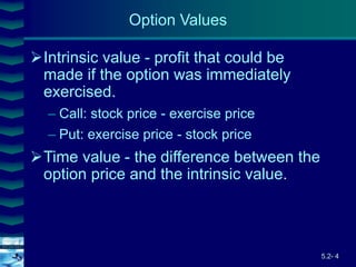
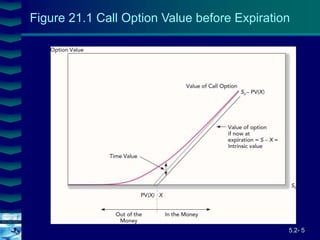
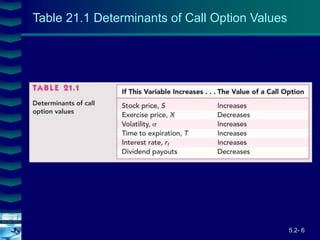
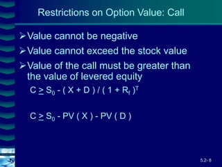
This document covers option valuation and pricing models. It introduces intrinsic and time value of options, restrictions on option values, and binomial and Black-Scholes option pricing models. The binomial model uses a multi-period tree approach to value options while the Black-Scholes model uses a partial differential equation and provides closed-form solutions. Both models require estimates of volatility to determine appropriate hedge ratios. The document also discusses hedging strategies using mispriced options.

1. Lesson 5
Option
Investments
Part 2: Option
Valuation
(Textbook chapter 21)
Cover image
Thanh Trúc – TCNH – UEL
5.2-1

2. 5.2- 2
Cover
image
 Option valuation: Introduction
 Restriction on option values
 Binomial option pricing
 Black-Scholes option valuation
Outline

3. 5.2- 3
Cover
image
Option valuation: Introduction

4. 5.2- 4
Cover
image
Intrinsic value - profit that could be
made if the option was immediately
exercised.
– Call: stock price - exercise price
– Put: exercise price - stock price
Time value - the difference between the
option price and the intrinsic value.
Option Values

5. 5.2- 5
Cover
image
Figure 21.1 Call Option Value before Expiration

6. 5.2- 6
Cover
image
Table 21.1 Determinants of Call Option Values

7. 5.2- 7
Cover
image
Restrictions on Option Value

8. 5.2- 8
Cover
image
Restrictions on Option Value: Call
Value cannot be negative
Value cannot exceed the stock value
Value of the call must be greater than
the value of levered equity
C > S0 - ( X + D ) / ( 1 + Rf )T
C > S0 - PV ( X ) - PV ( D )

9. 5.2- 9
Cover
image
Figure 21.2 Range of Possible Call Option
Values

10. 5.2- 10
Cover
image
Figure 21.3 Call Option Value as a Function of
the Current Stock Price

11. 5.2- 11
Cover
image
Figure 21.4 Put Option Values as a Function of
the Current Stock Price

12. 5.2- 12
Cover
image
Binomial Option Pricing

13. 5.2- 13
Cover
image
Binomial Option Pricing: Text Example
Page 735/1041

14. 5.2- 14
Cover
image
100
120
90
Stock Price
C
10
0
Call Option Value
X = 110
Binomial Option Pricing: Text Example

15. 5.2- 15
Cover
image
Alternative Portfolio
Buy 1 share of stock at $100
Borrow $81.82 (10% Rate)
Net outlay $18.18
Payoff
Value of Stock 90 120
Repay loan - 90 - 90
Net Payoff 0 30
18.18
30
0
Payoff Structure
is exactly 3 times
the Call
Binomial Option Pricing: Text Example

16. 5.2- 16
Cover
image
18.18
30
0
C
30
0
3C = $18.18
C = $6.06
Binomial Option Pricing: Text Example

17. 5.2- 17
Cover
image
Alternative Portfolio - one share of stock
and 3 calls written (X = 110)
Portfolio is perfectly hedged
Stock Value 90 120
Call Obligation 0 -30
Net payoff 90 90
Hence 100 - 3C = 81.82 or C = 6.06
Replication of Payoffs and Option Values

18. 5.2- 18
Cover
image
Why three call option?-The hedge ratio

19. 5.2- 19
Cover
image
Why three call option?-The hedge ratio

20. 5.2- 20
Cover
image
Arbitrage if the option is mispriced
What if the option is underpriced?
Reverse the arbitrage strategy

21. 5.2- 21
Cover
image
Generalizing the Two-State Approach
Assume that we can break the year into two six-
month segments.
In each six-month segment the stock could
increase by 10% or decrease by 5%.
Assume the stock is initially selling at 100.
Possible outcomes:
Increase by 10% twice
Decrease by 5% twice
Increase once and decrease once (2 paths).

22. 5.2- 22
Cover
image
Generalizing the Two-State Approach
100
110
121
95
90.25
104.50

23. 5.2- 23
Cover
image
Generalizing the Two-State Approach
Example: page 738/1041

24. 5.2- 24
Cover
image
Generalizing the Two-State Approach
Example: page 738/1041

25. 5.2- 25
Cover
image
Generalizing the Two-State Approach
Example: page 738/1041

26. 5.2- 26
Cover
image
Assume that we can break the year into
three intervals.
For each interval the stock could
increase by 5% or decrease by 3%.
Assume the stock is initially selling at
100.
Expanding to Consider Three Intervals

27. 5.2- 27
Cover
image
S
S +
S + +
S -
S - -
S + -
S + + +
S + + -
S + - -
S - - -
Expanding to Consider Three Intervals

28. 5.2- 28
Cover
image
Possible Outcomes with Three Intervals
Event Probability Stock Price
3 up 1/8 100 (1.05)3 =115.76
2 up 1 down 3/8 100 (1.05)2 (.97) =106.94
1 up 2 down 3/8 100 (1.05) (.97)2 = 98.79
3 down 1/8 100 (.97)3 = 91.27

29. 5.2- 29
Cover
image
Valuation of Put option
Excersice 9,10: page 766,767/1041

30. 5.2- 30
Cover
image
Valuation of Put option
Range of stock price: 80 – 130; range of Put option value 0 – 30
The hedge ratio = (30 – 0)/(130 – 80) = 3/5
The strategy: Buy 3 stocks at price of $100 and buy 5 put options
The payoffs:
Initial CFs S = 80 S = 130
Three stocks -300 240 390
5 put options -5P 150 0
300 + 5P 390 390
The value of the Portfolio = 390/1.1 = 354.545 = 300 + 5P
P = (354.545 – 300)/5 = $10.91
Put – Call Parity: S0 + P = PV(X) + C
C = S0 + P – PV(X) = 100 + 10.91 – 110/1.1 = $10.91

31. 5.2- 31
Cover
image
Figure 21.5 Probability Distributions

32. 5.2- 32
Cover
image
Black-Scholes Option Valuation

33. 5.2- 33
Cover
image
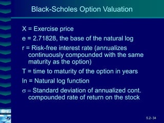
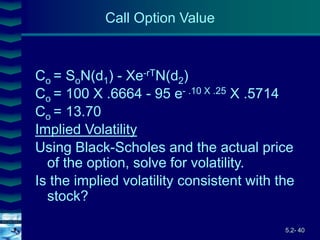
Co = SoN(d1) - Xe-rTN(d2)
d1 = [ln(So/X) + (r + 2/2)T] / (T1/2)
d2 = d1 + (T1/2)
where
Co = Current call option value.
So = Current stock price
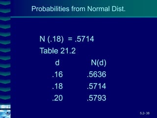
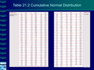
N(d) = probability that a random draw from a
normal dist. will be less than d.
Black-Scholes Option Valuation

34. 5.2- 34
Cover
image
X = Exercise price
e = 2.71828, the base of the natural log
r = Risk-free interest rate (annualizes
continuously compounded with the same
maturity as the option)
T = time to maturity of the option in years
ln = Natural log function
Standard deviation of annualized cont.
compounded rate of return on the stock
Black-Scholes Option Valuation

35. 5.2- 35
Cover
image
Figure 21.6 A Standard Normal Curve

36. 5.2- 36
Cover
image
So = 100 X = 95
r = .10 T = .25 (quarter)
= .50
d1 = [ln(100/95) + (.10+(5 2/2))] /
(5 .251/2)
= .43
d2 = .43 + ((5.251/2)
= .18
Call Option Example

37. 5.2- 37
Cover
image
N (.43) = .6664
Table 21.2
d N(d)
.42 .6628
.43 .6664 Interpolation
.44 .6700
Probabilities from Normal Dist

38. 5.2- 38
Cover
image
N (.18) = .5714
Table 21.2
d N(d)
.16 .5636
.18 .5714
.20 .5793
Probabilities from Normal Dist.

39. 5.2- 39
Cover
image
Table 21.2 Cumulative Normal Distribution

40. 5.2- 40
Cover
image
Co = SoN(d1) - Xe-rTN(d2)
Co = 100 X .6664 - 95 e- .10 X .25 X .5714
Co = 13.70
Implied Volatility
Using Black-Scholes and the actual price
of the option, solve for volatility.
Is the implied volatility consistent with the
stock?
Call Option Value

41. 5.2- 41
Cover
image
Spreadsheet 21.1 Spreadsheet to Calculate
Black-Scholes Option Values

42. 5.2- 42
Cover
image
Figure 21.7 Using Goal Seek to Find Implied
Volatility

43. 5.2- 43
Cover
image
Figure 21.8 Implied Volatility of the S&P 500

44. 5.2- 44
Cover
image
Black-Scholes Model with Dividends
The call option formula applies to stocks
that pay dividends.
One approach is to replace the stock
price with a dividend adjusted stock
price.
Replace S0 with S0 - PV (Dividends)

45. 5.2- 45
Cover
image
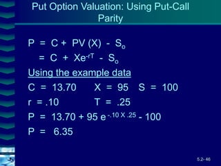
Put Value Using Black-Scholes
P = Xe-rT [1-N(d2)] - S0 [1-N(d1)]
Using the sample call data
S = 100 r = .10 X = 95 g = .5 T = .25
95e-10x.25(1-.5714)-100(1-.6664) = 6.35

46. 5.2- 46
Cover
image
P = C + PV (X) - So
= C + Xe-rT - So
Using the example data
C = 13.70 X = 95 S = 100
r = .10 T = .25
P = 13.70 + 95 e -.10 X .25 - 100
P = 6.35
Put Option Valuation: Using Put-Call
Parity

47. 5.2- 47
Cover
image
Hedging: Hedge ratio or delta
The number of stocks required to hedge against
the price risk of holding one option.
Call = N (d1)
Put = N (d1) - 1
Option Elasticity
Percentage change in the option’s value
given a 1% change in the value of the
underlying stock.
Using the Black-Scholes Formula

48. 5.2- 48
Cover
image
Figure 21.9 Call Option Value and Hedge Ratio

49. 5.2- 49
Cover
image
Buying Puts - results in downside
protection with unlimited upside
potential.
Limitations
– Tracking errors if indexes are used for the
puts.
– Maturity of puts may be too short.
– Hedge ratios or deltas change as stock
values change.
Portfolio Insurance

50. 5.2- 50
Cover
image
Figure 21.10 Profit on a Protective Put Strategy

51. 5.2- 51
Cover
image
Figure 21.11 Hedge Ratios Change as the
Stock Price Fluctuates

52. 5.2- 52
Cover
image
Figure 21.12 S&P 500 Cash-to-Futures Spread
in Points at 15 Minute Intervals

53. 5.2- 53
Cover
image
Hedging On Mispriced Options
Option value is positively related to
volatility:
If an investor believes that the volatility
that is implied in an option’s price is too
low, a profitable trade is possible.
Profit must be hedged against a decline
in the value of the stock.
Performance depends on option price
relative to the implied volatility.

54. 5.2- 54
Cover
image
Hedging and Delta
The appropriate hedge will depend on the
delta.
Recall the delta is the change in the value
of the option relative to the change in
the value of the stock.
Delta =
Change in the value of the option
Change of the value of the stock

55. 5.2- 55
Cover
image
Mispriced Option: Text Example
Implied volatility = 33%
Investor believes volatility should = 35%
Option maturity = 60 days
Put price P = $4.495
Exercise price and stock price = $90
Risk-free rate r = 4%
Delta = -.453

56. 5.2- 56
Cover
image
Table 21.3 Profit on a Hedged Put Portfolio

57. 5.2- 57
Cover
image
Table 21.4 Profits on Delta-Neutral Options
Portfolio

58. 5.2- 58
Cover
image
Figure 21.13 Implied Volatility of the S&P 500
Index as a Function of Exercise Price