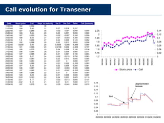
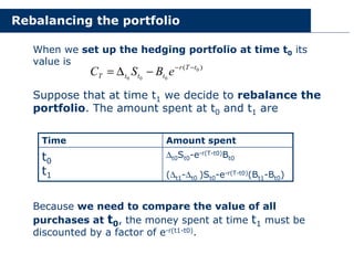
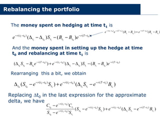
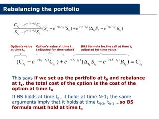
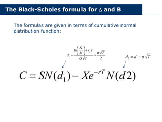
The Black-Scholes Formula
Dr. Guillermo López Dumrauf
dumrauf@fibertel.com.ar
Black & Scholes
Copyright © 2006 by Dr. Guillermo López Dumrauf.
No part of this publication may be reproduced, stored in a retrieval system, or transmitted in any form or by any means —
electronic, mechanical, photocopying, recording, or otherwise — without the permission of Dr. Guillermo López Dumrauf
This document provides an outline of a presentation and is incomplete without the accompanying oral commentary and discussion.
Hedging
If you writing a call option, you are exposed to the
risk of the stock price rising above the strike price at
expiration
In order to cover the call, you need at expiration,
cash equal to the difference between the current price
of the stock and the strike price of the option (ST-K)
In Black-Scholes, the hedge is a portfolio
compounded with some shares of the underlying
stock and some riskless assets (US T-Bonds)
How much of each to put in the hedge is the
key to determining the option’s value.
Perfect hedge
A perfect hedge always pays exactly the amount
necessary to cover the option.
Payoff replication:
• if the option expires in the money, the hedge
provides exactly the amount necessary to cover
the call
• if the option expires out of the money the
hedge will be worth nothing
Dynamic hedging
Dynamic hedging is a trading strategy
which replicates the payoff of the option
throughout its life (creating a perfect
hedge)
It has a fixed and known total cost
Dynamic hedging is a process for managing
the risk of options and it is important for
explaining an option’s value.
Dynamic hedging
Black-Scholes hedging is determined by the weights
of the hedging portfolio. Because the parameters
of the formula are constantly changing, the
hedging portfolio must be constantly updated to
reflect the new weights…
The portfolio which doesn’t reflects the current Black-
Scholes weights is out of balance. The process to
keeping the portfolio in balance is called rebalancing
If the hedging strategy is performed correctly,
the value of the portfolio will be equal to the
value of the option at all times…
Costs of the hedging
1. Set-up cost (initial cash flows associated with
the hedging strategy)
2. Maintenance costs: infusion and transaction
costs (costs associated with rebalancing the
hedge, e.g. buy more share of stock or bonds)
In addition, there are:
• fees and taxes associated with making the
transactions
• costs resulting from the bid-ask spread and
• the inability to execute trades at exactly the price
specified by the strategy
Self-Financing Dynamic Hedging
A hedging strategy whose total cost at any
time (excluding transaction costs) is equal
to set-up costs is called self-financing.
The coin-tossing example
A gambler decides making a bet of
$100.000 He needs 3 faces to win
12.500!25.000
25.000!50.000
50.000!100.000
The Delta of an option
The Delta of an option is the rate of the
change in the option price with respect to
the change in the stock price
When we look at changes in the value of an
option, we are interested in changes relative to
the underlying stock price.
If the price of the stock changes $1, what will be
the change in the option’s value?
The Delta of an option
• Option is deep in the money and near
expiration: the delta is close to one, so there is a
dollar for dollar relationship between movements of
the spot price and movements of the option’s value
• Option is deep out of the money and near
expiration: the delta is close to zero (because the
option’s value is absolutely insensitive to changes in the stock
price) and it will be worth almost nothing
Implicit in the B&S model there is only factor of
uncertainty in the value of an option: volatility
In truth, the uncertainty implicit in an option is more
complicated than this.
The Delta of an option
Real world is more complicated: the dynamic of stock
price is more complicated than a geometric brownian
motion
Jump risk: if there is a probability of stock price will
unexpectedly jump downward, this can change the option’s
value even when the spot price does not change (Brownian
motion model does not include this effect)
In principle, we can observe this jump comparing the
spot price and option value at some time t0 , doing the
same at a later time t1
Because the price of the option is not controlled by the stock
price alone, this may note give an accurate estimate of the
delta of the option
Even if we ignore probabilities of jumps and changing volatility, the value of
the options does change as time elapses (see parameter theta)
The Delta of an option
1. Time change and
2. Stock price change
In the B&S world, stock price are supposed to
follow a GBM with constant volatility and the
option’s value changes for only two reasons:
We can use an approximation to the delta of
the option: the actual rate of change in the
value of the option with respect to the change
in the stock price...
The Delta of an option
How the formula works in the real world?
Example:
S0=1,87; c0=0,059
S1=1,89; c1=0,06
The value of the delta is 0,05
The numerator says the time adjusted change in the price
of the option was $ 0,02 while the time adjusted change
in the stock price was $0,001
The ratio says that for every $1 change in the stock price,
there was an approximately $0,05 in the value of the
option
05
,
0
02
,
0
001
,
0
87
,
1
89
,
1
059
,
0
06
,
0
)
365
/
1
(
047
,
0
)
365
/
1
(
047
,
0
)
(
)
(
1
0
1
0
1
0
1
0
≅
=
−
−
=
−
−
=
∆ −
−
−
−
e
e
S
e
S
C
e
C
t
t
t
r
t
t
t
t
r
t
Call evolution for Transener
0
0,02
0,04
0,06
0,08
0,1
0,12
0,14
0,16
0,18
20/03/06 22/03/06 24/03/06 26/03/06 28/03/06 30/03/06 01/04/06 03/04/06
Approximated
formula
Call
Date Stock price Call Days to maturity Var S Var Call Delta Call (formula)
14/03/06 1,82 0,042 38
21/03/06 1,89 0,06 31 0,07 0,018 0,257
22/03/06 1,87 0,059 30 -0,02 -0,001 0,050 0,055
23/03/06 1,89 0,06 29 0,02 0,001 0,050 0,060
23/03/06 1,87 0,053 29 -0,02 -0,007 0,350 0,059
25/03/06 1,86 0,05 27 -0,01 -0,003 0,300 0,050
25/03/06 1,9 0,055 27 0,04 0,005 0,125 0,062
27/03/06 1,92 0,068 25 0,02 0,013 0,650 0,058
27/03/06 1,9209 0,06 25 0,0009 -0,008 -8,889 0,069
27/03/06 1,91 0,069 25 -0,0109 0,009 -0,826 0,157
27/03/06 1,95 0,075 25 0,04 0,006 0,150 0,036
27/03/06 1,96 0,084 25 0,01 0,009 0,900 0,077
27/03/06 1,97 0,085 25 0,01 0,001 0,100 0,093
28/03/06 1,95 0,07 24 -0,02 -0,015 0,750 0,083
28/03/06 1,97 0,083 24 0,02 0,013 0,650 0,085
28/03/06 1,96 0,083 24 -0,01 0 0,000 0,077
28/03/06 1,95 0,085 24 -0,01 0,002 -0,200 0,083
28/03/06 1,97 0,09 24 0,02 0,005 0,250 0,081
28/03/06 1,96 0,087 24 -0,01 -0,003 0,300 0,088
29/03/06 1,97 0,085 23 0,01 -0,002 -0,200 0,090
29/03/06 1,98 0,085 23 0,01 0 0,000 0,083
30/03/06 1,99 0,09 22 0,01 0,005 0,500 0,085
30/03/06 2,03 0,123 22 0,04 0,033 0,825 0,110
31/03/06 2,01 0,11 21 -0,02 -0,013 0,650 0,107
31/03/06 2,02 0,12 21 0,01 0,01 1,000 0,117
02/04/06 1,97 0,075 19 -0,05 -0,045 0,900 0,070
1,7
1,75
1,8
1,85
1,9
1,95
2
2,05
0
0,02
0,04
0,06
0,08
0,1
0,12
0,14
Stock price Call
The approximate formula
The formula is a good approximation because:
1. If we choose a time t1 very close to time t0
and apply the formula, then we obtain values
for the delta that are very close to the actual
value of the delta at time t0
2. Each time we substitute the approximate
value of the delta for the real value, we
produce a small error. But these small errors
do not accumulate, and do not make our
approximation useless!!
Delta – approximate formula
What makes the formula an approximation is the fact that
we compare the change in the option price to the change
in the stock price over small period of time.
If all times are infinitesimally close, we get
a formula that is no longer approximate but
is precisely correct...
What if the denominator of the formula is zero?
This does not invalidate the formula, because according to the BM model,
the probability that the stock price at time t1 will be exactly equal to… is
zero (the probability of any given “event”is always zero, only ranges of
events matter in probability theory) Of course, in reality it can happen.
The Black-Scholes hedging strategy
If we know the delta of a european call or put
option, we can hedge the option and
determine its theoretical value
The assumptions behind the Black-Scholes
formula play a key role in determining the
value of an option. Identifying how relaxing
them is an important part of understanding the
Black-Scholes method
Hedging strategy in Black-Scholes
A very important part is to understand how the
formula translates into a hedging strategy
that replicates the payoff of the option
Then, no-arbitrage assumptions ensures
that the value of the option is equal to the
cost of the hedging strategy
Hedging strategy in Black-Scholes
)
( t
T
r
t
t
t e
B
S −
−
−
∆
The value of the hedging portfolio at time t, is the
SAME as the B&S Formula for the option’s value
Once the hedging is set up, the next step is
to maintain the hedge…
In order to keep the portfolio in balance, we will
have to continuously monitor the values of ∆ and
B, buying or selling shares…
In order to ensure the strategy is self-rebalancing
we want the rebalancing costs at every step to be
as close to zero as possible
Hedging strategy in Black-Scholes
In reality, the hedging strategy is used to
hedge an option not on a single share of stock
but on some larger number of shares (In
Argentina, a standard option contract is on 100 shares of
the underlying)
Since delta is a number between 0 and 1,
it represents the percentage of the lot of
shares that should be purchased…
The hedging strategy is self-financing
In BS world there is no transactions costs, so
Set up costs=value of option=total cost of hedging
Therefore, set-up costs equal the total cost of hedging,
which implies that the maintenance cost of hedging
must equal zero and the portfolio is self-financing
If the BS formula holds, then the hedging strategy must
be self-financing. It would be more convincing if we
started with the hedging strategy and then showed that
it replicates the payoff of the option and is self-financing
Rebalancing the portfolio
When we set up the hedging portfolio at time t0 its
value is
Suppose that at time t1 we decide to rebalance the
portfolio. The amount spent at t0 and t1 are
∆t0St0-e-r(T-t0)Bt0
(∆t1-∆t0 )St0-e-r(T-t0)(Bt1-Bt0)
t0
t1
Amount spent
Time
)
( 0
0
0
0
t
T
r
t
t
t
T e
B
S
C −
−
−
∆
=
Because we need to compare the value of all
purchases at t0, the money spent at time t1 must be
discounted by a factor of e-r(t1-t0).
Rebalancing the portfolio
)
(
)
( 0
0
1
1
0
1
0
1
)
(
)
( t
T
r
t
t
t
t
t
t
t
r
e
B
B
S
e −
−
−
−
−
−
∆
−
∆
)
(
)
( 0
1
0
0
1
1
0
1 )
(
)
(
)
(
t
t
t
T
r
t
t
t
T
r
t
t
r
B
B
e
B
B
e
e −
=
− −
−
−
−
−
−
The money spent on hedging at time t1 is
And the money spent in setting up the hedge at time
t0 and rebalancing at time t1 is
)
(
)
(
)
( 0
0
1
1
0
1
0
1
0
0
0
0
)
(
)
(
)
( t
T
r
t
t
t
t
t
t
t
r
t
T
r
t
t
t e
B
B
S
e
e
B
S −
−
−
−
−
−
−
−
∆
−
∆
+
−
∆
Rearranging this a bit, we obtain
)
(
)
( 1
1
1
1
0
1
1
0
1
0
0
)
(
)
(
)
(
t
t
T
r
t
t
t
t
r
t
t
t
r
t
t B
e
S
e
S
e
S −
−
−
−
−
−
−
∆
+
−
∆
Replacing ∆t0 in the last expression for the approximate
delta, we have
)
(
)
( 1
1
1
1
0
1
1
0
1
0
1
0
1
0
1
0
1
0 )
(
)
(
)
(
)
(
)
(
t
t
T
r
t
t
t
t
r
t
t
t
r
t
t
t
t
r
t
t
t
t
r
t
B
e
S
e
S
e
S
S
e
S
C
e
C −
−
−
−
−
−
−
−
−
−
−
∆
+
−
−
−
Rebalancing the portfolio
)
(
)
( 1
1
1
1
0
1
1
0
1
0
1
0
1
0
1
0
1
0 )
(
)
(
)
(
)
(
)
(
t
t
T
r
t
t
t
t
r
t
t
t
r
t
t
t
t
r
t
t
t
t
r
t
B
e
S
e
S
e
S
S
e
S
C
e
C −
−
−
−
−
−
−
−
−
−
−
∆
+
−
−
−
0
1
1
1
1
0
1
1
0
1
0
)
(
)
( )
(
)
(
)
(
t
t
t
T
r
t
t
t
t
r
t
t
t
r
t C
B
e
S
e
C
e
C =
−
∆
+
− −
−
−
−
−
−
B&S formula for the call at time t1
adjusted for time value
Option’s value at time t1
(adjusted for time value)
Option’s value
at time t0
This says if we set up the portfolio at t0 and rebalance
at t1, the total cost of the option is the cost of the
option at time t0
If BS holds at time t0 , it holds at time N-1; the same
arguments imply that it holds at time tN-2, tN-3….so BS
formula must hold at time t0
The Black-Scholes formula for ∆
∆
∆
∆ and B
The formulas are given in terms of cumulative normal
distribution function:
2
ln
1
T
T
T
r
X
S
d
f
σ
σ
+
+






= T
d
d σ
−
= 1
2
)
2
(
)
( 1 d
N
Xe
d
SN
C rT
−
−
=
Black-Scholes and the Brownian Motion Model
Computing the probability that C expires in the
money is equivalent to computing the probability that K
ST ≥
The return on S from time t to time T is given by 







t
T
S
S
ln
This return is a random variable with mean )
(
2
2
t
T
r −








−
σ
n
And standard deviation t
-
T
σ
Therefore, the random variable is given by
t
T
t
T
r
S
S
t
T
−
−








−
−








σ
σ
)
(
2
ln
2
This is normally distributed, with mean zero
and standard deviation 1
Black-Scholes and the Brownian Motion Model
Now, we transform the equation ST≥K dividing both sides
by St, taking logarithms, substracting r - σ
σ
σ
σ2/2 (T-t) and
finally, by dividing by t
-
T
σ
t
T
t
T
r
S
K
t
T
t
T
r
S
S
t
t
T
−
−








−
−








≥
−
−








−
−








σ
σ
σ
σ
)
(
2
ln
)
(
2
ln
2
2
Because we want an expression with “less than or
equal” (to use the cumulative normal distribution) we
negate this equation and obtain:
t
T
t
T
r
K
S
t
T
t
T
r
S
S t
T
t
−
−








−
+






≤
−
−








−
+








σ
σ
σ
σ
)
(
2
ln
)
(
2
ln
2
2
Black-Scholes and the Brownian Motion Model
For the original statement to be true (ST≥K) then the random
variable on the left-hand side of equation must be less than
or equal to the value on the right-hand side
The probability the inequality holds is exactly given by the
cumulative normal distribution of the right-hand side, so
the probability that C will expire in the money is
t
T
t
T
r
K
S
t
T
t
T
r
S
S t
T
t
−
−








−
+






≤
−
−








−
+








σ
σ
σ
σ
)
(
2
ln
)
(
2
ln
2
2














−
−








−
+






=
≤
t
T
t
T
r
K
S
N
K
S
P
t
T
σ
σ
)
(
2
ln
)
(
2
Excercises
1. Using B&S formula, calculate the fair value for a
call option on Petrobras, for different strike prices.
Today is 7/4/06 and the annual risk free rate is
4,9%. Then compare this value with the option
market value.
2. Calculate the implied volatility for K=4
Option
market
value
Stock
price

blackscholesformula.pdf

  • 1.
    The Black-Scholes Formula Dr.Guillermo López Dumrauf dumrauf@fibertel.com.ar Black & Scholes Copyright © 2006 by Dr. Guillermo López Dumrauf. No part of this publication may be reproduced, stored in a retrieval system, or transmitted in any form or by any means — electronic, mechanical, photocopying, recording, or otherwise — without the permission of Dr. Guillermo López Dumrauf This document provides an outline of a presentation and is incomplete without the accompanying oral commentary and discussion.
  • 2.
    Hedging If you writinga call option, you are exposed to the risk of the stock price rising above the strike price at expiration In order to cover the call, you need at expiration, cash equal to the difference between the current price of the stock and the strike price of the option (ST-K) In Black-Scholes, the hedge is a portfolio compounded with some shares of the underlying stock and some riskless assets (US T-Bonds) How much of each to put in the hedge is the key to determining the option’s value.
  • 3.
    Perfect hedge A perfecthedge always pays exactly the amount necessary to cover the option. Payoff replication: • if the option expires in the money, the hedge provides exactly the amount necessary to cover the call • if the option expires out of the money the hedge will be worth nothing
  • 4.
    Dynamic hedging Dynamic hedgingis a trading strategy which replicates the payoff of the option throughout its life (creating a perfect hedge) It has a fixed and known total cost Dynamic hedging is a process for managing the risk of options and it is important for explaining an option’s value.
  • 5.
    Dynamic hedging Black-Scholes hedgingis determined by the weights of the hedging portfolio. Because the parameters of the formula are constantly changing, the hedging portfolio must be constantly updated to reflect the new weights… The portfolio which doesn’t reflects the current Black- Scholes weights is out of balance. The process to keeping the portfolio in balance is called rebalancing If the hedging strategy is performed correctly, the value of the portfolio will be equal to the value of the option at all times…
  • 6.
    Costs of thehedging 1. Set-up cost (initial cash flows associated with the hedging strategy) 2. Maintenance costs: infusion and transaction costs (costs associated with rebalancing the hedge, e.g. buy more share of stock or bonds) In addition, there are: • fees and taxes associated with making the transactions • costs resulting from the bid-ask spread and • the inability to execute trades at exactly the price specified by the strategy
  • 7.
    Self-Financing Dynamic Hedging Ahedging strategy whose total cost at any time (excluding transaction costs) is equal to set-up costs is called self-financing. The coin-tossing example A gambler decides making a bet of $100.000 He needs 3 faces to win 12.500!25.000 25.000!50.000 50.000!100.000
  • 8.
    The Delta ofan option The Delta of an option is the rate of the change in the option price with respect to the change in the stock price When we look at changes in the value of an option, we are interested in changes relative to the underlying stock price. If the price of the stock changes $1, what will be the change in the option’s value?
  • 9.
    The Delta ofan option • Option is deep in the money and near expiration: the delta is close to one, so there is a dollar for dollar relationship between movements of the spot price and movements of the option’s value • Option is deep out of the money and near expiration: the delta is close to zero (because the option’s value is absolutely insensitive to changes in the stock price) and it will be worth almost nothing Implicit in the B&S model there is only factor of uncertainty in the value of an option: volatility In truth, the uncertainty implicit in an option is more complicated than this.
  • 10.
    The Delta ofan option Real world is more complicated: the dynamic of stock price is more complicated than a geometric brownian motion Jump risk: if there is a probability of stock price will unexpectedly jump downward, this can change the option’s value even when the spot price does not change (Brownian motion model does not include this effect) In principle, we can observe this jump comparing the spot price and option value at some time t0 , doing the same at a later time t1 Because the price of the option is not controlled by the stock price alone, this may note give an accurate estimate of the delta of the option Even if we ignore probabilities of jumps and changing volatility, the value of the options does change as time elapses (see parameter theta)
  • 11.
    The Delta ofan option 1. Time change and 2. Stock price change In the B&S world, stock price are supposed to follow a GBM with constant volatility and the option’s value changes for only two reasons: We can use an approximation to the delta of the option: the actual rate of change in the value of the option with respect to the change in the stock price...
  • 12.
    The Delta ofan option How the formula works in the real world? Example: S0=1,87; c0=0,059 S1=1,89; c1=0,06 The value of the delta is 0,05 The numerator says the time adjusted change in the price of the option was $ 0,02 while the time adjusted change in the stock price was $0,001 The ratio says that for every $1 change in the stock price, there was an approximately $0,05 in the value of the option 05 , 0 02 , 0 001 , 0 87 , 1 89 , 1 059 , 0 06 , 0 ) 365 / 1 ( 047 , 0 ) 365 / 1 ( 047 , 0 ) ( ) ( 1 0 1 0 1 0 1 0 ≅ = − − = − − = ∆ − − − − e e S e S C e C t t t r t t t t r t
  • 13.
    Call evolution forTransener 0 0,02 0,04 0,06 0,08 0,1 0,12 0,14 0,16 0,18 20/03/06 22/03/06 24/03/06 26/03/06 28/03/06 30/03/06 01/04/06 03/04/06 Approximated formula Call Date Stock price Call Days to maturity Var S Var Call Delta Call (formula) 14/03/06 1,82 0,042 38 21/03/06 1,89 0,06 31 0,07 0,018 0,257 22/03/06 1,87 0,059 30 -0,02 -0,001 0,050 0,055 23/03/06 1,89 0,06 29 0,02 0,001 0,050 0,060 23/03/06 1,87 0,053 29 -0,02 -0,007 0,350 0,059 25/03/06 1,86 0,05 27 -0,01 -0,003 0,300 0,050 25/03/06 1,9 0,055 27 0,04 0,005 0,125 0,062 27/03/06 1,92 0,068 25 0,02 0,013 0,650 0,058 27/03/06 1,9209 0,06 25 0,0009 -0,008 -8,889 0,069 27/03/06 1,91 0,069 25 -0,0109 0,009 -0,826 0,157 27/03/06 1,95 0,075 25 0,04 0,006 0,150 0,036 27/03/06 1,96 0,084 25 0,01 0,009 0,900 0,077 27/03/06 1,97 0,085 25 0,01 0,001 0,100 0,093 28/03/06 1,95 0,07 24 -0,02 -0,015 0,750 0,083 28/03/06 1,97 0,083 24 0,02 0,013 0,650 0,085 28/03/06 1,96 0,083 24 -0,01 0 0,000 0,077 28/03/06 1,95 0,085 24 -0,01 0,002 -0,200 0,083 28/03/06 1,97 0,09 24 0,02 0,005 0,250 0,081 28/03/06 1,96 0,087 24 -0,01 -0,003 0,300 0,088 29/03/06 1,97 0,085 23 0,01 -0,002 -0,200 0,090 29/03/06 1,98 0,085 23 0,01 0 0,000 0,083 30/03/06 1,99 0,09 22 0,01 0,005 0,500 0,085 30/03/06 2,03 0,123 22 0,04 0,033 0,825 0,110 31/03/06 2,01 0,11 21 -0,02 -0,013 0,650 0,107 31/03/06 2,02 0,12 21 0,01 0,01 1,000 0,117 02/04/06 1,97 0,075 19 -0,05 -0,045 0,900 0,070 1,7 1,75 1,8 1,85 1,9 1,95 2 2,05 0 0,02 0,04 0,06 0,08 0,1 0,12 0,14 Stock price Call
  • 14.
    The approximate formula Theformula is a good approximation because: 1. If we choose a time t1 very close to time t0 and apply the formula, then we obtain values for the delta that are very close to the actual value of the delta at time t0 2. Each time we substitute the approximate value of the delta for the real value, we produce a small error. But these small errors do not accumulate, and do not make our approximation useless!!
  • 15.
    Delta – approximateformula What makes the formula an approximation is the fact that we compare the change in the option price to the change in the stock price over small period of time. If all times are infinitesimally close, we get a formula that is no longer approximate but is precisely correct... What if the denominator of the formula is zero? This does not invalidate the formula, because according to the BM model, the probability that the stock price at time t1 will be exactly equal to… is zero (the probability of any given “event”is always zero, only ranges of events matter in probability theory) Of course, in reality it can happen.
  • 16.
    The Black-Scholes hedgingstrategy If we know the delta of a european call or put option, we can hedge the option and determine its theoretical value The assumptions behind the Black-Scholes formula play a key role in determining the value of an option. Identifying how relaxing them is an important part of understanding the Black-Scholes method
  • 17.
    Hedging strategy inBlack-Scholes A very important part is to understand how the formula translates into a hedging strategy that replicates the payoff of the option Then, no-arbitrage assumptions ensures that the value of the option is equal to the cost of the hedging strategy
  • 18.
    Hedging strategy inBlack-Scholes ) ( t T r t t t e B S − − − ∆ The value of the hedging portfolio at time t, is the SAME as the B&S Formula for the option’s value Once the hedging is set up, the next step is to maintain the hedge… In order to keep the portfolio in balance, we will have to continuously monitor the values of ∆ and B, buying or selling shares… In order to ensure the strategy is self-rebalancing we want the rebalancing costs at every step to be as close to zero as possible
  • 19.
    Hedging strategy inBlack-Scholes In reality, the hedging strategy is used to hedge an option not on a single share of stock but on some larger number of shares (In Argentina, a standard option contract is on 100 shares of the underlying) Since delta is a number between 0 and 1, it represents the percentage of the lot of shares that should be purchased…
  • 20.
    The hedging strategyis self-financing In BS world there is no transactions costs, so Set up costs=value of option=total cost of hedging Therefore, set-up costs equal the total cost of hedging, which implies that the maintenance cost of hedging must equal zero and the portfolio is self-financing If the BS formula holds, then the hedging strategy must be self-financing. It would be more convincing if we started with the hedging strategy and then showed that it replicates the payoff of the option and is self-financing
  • 21.
    Rebalancing the portfolio Whenwe set up the hedging portfolio at time t0 its value is Suppose that at time t1 we decide to rebalance the portfolio. The amount spent at t0 and t1 are ∆t0St0-e-r(T-t0)Bt0 (∆t1-∆t0 )St0-e-r(T-t0)(Bt1-Bt0) t0 t1 Amount spent Time ) ( 0 0 0 0 t T r t t t T e B S C − − − ∆ = Because we need to compare the value of all purchases at t0, the money spent at time t1 must be discounted by a factor of e-r(t1-t0).
  • 22.
    Rebalancing the portfolio ) ( ) (0 0 1 1 0 1 0 1 ) ( ) ( t T r t t t t t t t r e B B S e − − − − − − ∆ − ∆ ) ( ) ( 0 1 0 0 1 1 0 1 ) ( ) ( ) ( t t t T r t t t T r t t r B B e B B e e − = − − − − − − − The money spent on hedging at time t1 is And the money spent in setting up the hedge at time t0 and rebalancing at time t1 is ) ( ) ( ) ( 0 0 1 1 0 1 0 1 0 0 0 0 ) ( ) ( ) ( t T r t t t t t t t r t T r t t t e B B S e e B S − − − − − − − − ∆ − ∆ + − ∆ Rearranging this a bit, we obtain ) ( ) ( 1 1 1 1 0 1 1 0 1 0 0 ) ( ) ( ) ( t t T r t t t t r t t t r t t B e S e S e S − − − − − − − ∆ + − ∆ Replacing ∆t0 in the last expression for the approximate delta, we have ) ( ) ( 1 1 1 1 0 1 1 0 1 0 1 0 1 0 1 0 1 0 ) ( ) ( ) ( ) ( ) ( t t T r t t t t r t t t r t t t t r t t t t r t B e S e S e S S e S C e C − − − − − − − − − − − ∆ + − − −
  • 23.
    Rebalancing the portfolio ) ( ) (1 1 1 1 0 1 1 0 1 0 1 0 1 0 1 0 1 0 ) ( ) ( ) ( ) ( ) ( t t T r t t t t r t t t r t t t t r t t t t r t B e S e S e S S e S C e C − − − − − − − − − − − ∆ + − − − 0 1 1 1 1 0 1 1 0 1 0 ) ( ) ( ) ( ) ( ) ( t t t T r t t t t r t t t r t C B e S e C e C = − ∆ + − − − − − − − B&S formula for the call at time t1 adjusted for time value Option’s value at time t1 (adjusted for time value) Option’s value at time t0 This says if we set up the portfolio at t0 and rebalance at t1, the total cost of the option is the cost of the option at time t0 If BS holds at time t0 , it holds at time N-1; the same arguments imply that it holds at time tN-2, tN-3….so BS formula must hold at time t0
  • 24.
    The Black-Scholes formulafor ∆ ∆ ∆ ∆ and B The formulas are given in terms of cumulative normal distribution function: 2 ln 1 T T T r X S d f σ σ + +       = T d d σ − = 1 2 ) 2 ( ) ( 1 d N Xe d SN C rT − − =
  • 25.
    Black-Scholes and theBrownian Motion Model Computing the probability that C expires in the money is equivalent to computing the probability that K ST ≥ The return on S from time t to time T is given by         t T S S ln This return is a random variable with mean ) ( 2 2 t T r −         − σ n And standard deviation t - T σ Therefore, the random variable is given by t T t T r S S t T − −         − −         σ σ ) ( 2 ln 2 This is normally distributed, with mean zero and standard deviation 1
  • 26.
    Black-Scholes and theBrownian Motion Model Now, we transform the equation ST≥K dividing both sides by St, taking logarithms, substracting r - σ σ σ σ2/2 (T-t) and finally, by dividing by t - T σ t T t T r S K t T t T r S S t t T − −         − −         ≥ − −         − −         σ σ σ σ ) ( 2 ln ) ( 2 ln 2 2 Because we want an expression with “less than or equal” (to use the cumulative normal distribution) we negate this equation and obtain: t T t T r K S t T t T r S S t T t − −         − +       ≤ − −         − +         σ σ σ σ ) ( 2 ln ) ( 2 ln 2 2
  • 27.
    Black-Scholes and theBrownian Motion Model For the original statement to be true (ST≥K) then the random variable on the left-hand side of equation must be less than or equal to the value on the right-hand side The probability the inequality holds is exactly given by the cumulative normal distribution of the right-hand side, so the probability that C will expire in the money is t T t T r K S t T t T r S S t T t − −         − +       ≤ − −         − +         σ σ σ σ ) ( 2 ln ) ( 2 ln 2 2               − −         − +       = ≤ t T t T r K S N K S P t T σ σ ) ( 2 ln ) ( 2
  • 28.
    Excercises 1. Using B&Sformula, calculate the fair value for a call option on Petrobras, for different strike prices. Today is 7/4/06 and the annual risk free rate is 4,9%. Then compare this value with the option market value. 2. Calculate the implied volatility for K=4 Option market value Stock price