S’ = 24.978 Safety Stock = Z * S’ Safety Stock = 1.645 * 24.978 = 512 cases Therefore, the safety stock required for a 95% stock protection level is 512 cases. Cabot Food Company 11 University of Tennessee Appendix E: Stock Protection Level Stock Protection Level = 95% Corresponding z-score (Z) = 1.645 Safety Stock (SS) = 512 cases Average Daily Demand (d) = 101.053 cases Lead Time (LT) = 5 days Inventory Level at 95% Stock Protection: Inventory = Average Daily Demand * Lead

1. Louisiana
Processing Luncheon Meat
Since 1974
Cabot Food Company
Inventory Management for Enhanced Performance
Andy Wyatt
Jordan Drummel
Paul Kapcar
December 3, 2010

2. University of Tennessee
Table of Contents
Background
1
Contribution and Cost of Good Sold (COGS) per Case
2
2006 Sales Projections
2
Standard Deviation of Sales
3
Safety Stock
3
Stock Protection Level Variation
3
Reorder Points
4
Expected Service Level
4
Total Cost of Inventory
5
Appendix A: Contribution and Cost of Goods Sold
6
Appendix B: Sales Volume and Order Quantity
7
Appendix C: Standard Deviation of Sales
9
Appendix D: Safety Stock
11
Appendix E: Stock Protection Level
12
Appendix F: Reorder Point
13
Appendix G: Service Levels
14
Appendix H: Total Cost
15
Name of report
i

3. University of Tennessee - Logistics 411
Cabot Food Company :
Inventory Management for Enhanced Performance
Background
Cabot is a well-established foods company specializing in luncheon meat and has been selling its products throughout
the United States since 1974. Though the company sold a variety of products, its competitive strength lay in two main
lines of luncheon meat: Lunch Delight and Tasty. 1
Lunch Delight Sales Projection Data
2004 2005 2006
$6,000,000 $6,900,000 $72,000,000
Actual +15% +20%
Approximately 50% of the sales revenue was attributable to direct variable costs for both the brands; 75% of the direct
variable costs were estimated to be actual meat costs (again for both the brands). These costing percentages were
expected to hold for the next few years. Lunch Delight was sold to retail outlets for $9.5 per pound.
Profit Actual Meat Costs Other Variable Costs
Sales Revenue
50%
13% 38%
Approximately 50% of the sales revenue was attributable to direct variable costs for both the brands
1 Cabot Food Company by Rajiv P. Dant and Daniel L. Kurfees, Appalachian State University. Revised Spring 2007 by Funda Sahin.
Cabot Food Company
1

4. University of Tennessee - Logistics 411
Contribution and Cost of Good Sold (COGS) per Case
Cabot sells Lunch Delight to retailers at $9.50 per pound, shipments are packed in 30 lb. cases, resulting in a $285
cases. Cabot managers estimate 50% of sales revenue is attributable to direct variable costs, and of the direct variable
costs 75% are the actual meat costs. The current cost approximations are expected to hold for the next few years.
Under these approximations, each case sold has a 50% contribution margin; thus, $142.50 out of every $285 in revenue
remains after variable costs are deducted (see Appendix A for detailed calculation).
Contribution Costs of Good Sold Other Variable Costs
Per Case Breakdown
$106.88 $35.63
$142.50
2006 Sales Projections
As mentioned previously, the 2005 sales indicated a 15% and a 20% growth over the 2004 sales level for Lunch Delight
for 2005 and 2006, respectively. Lunch Delight is shipped in 30 pound cases at a sell price of $285; each order placed
incurs a $40 ordering cost and a 20% inventory carrying cost. Cabot places orders in simple economic order quantities.
2(D)(S)
(I)(C)
Formula utilized for Economic Order Quantity2
D= Demand (annual), S = Order Placement Cost, I = Inventory Carrying cost and C = Product cost
Lunch Delight 2006 Sales Volume Projections (see Appendix B for detailed calculation):
Annual Volume (cases) Average Daily Volume Economic Order Quantity
25,264 101 308
2Commonly termed EOQ
Cabot Food Company
2

5. University of Tennessee - Logistics 411
Standard Deviation of Sales
Cabot’s Lunch Delight product has a 25 case per day standard deviation of sales (see Appendix C for detailed
calculation). The standard deviation of sales was found using data provided by the sales department regarding
distribution of daily demand from retailers for 2005 on reviewing the last 50 working days:
Demand for Lunch Delight During Lead Time, 2005
Cases Frequency
200 10
202 11
250 40
260 11
268 10
Cabot advised utilization of the following equation for standard deviation of sales calculation:
Formula utilized for standard deviation calculation 3
f= frequency and d= difference
Safety Stock
Cabot’s Lunch Delight product is transported from Texas to Louisiana with an average transit time of 5 days, however
due to the selection of rail as the mode of transportation, Cabot experiences lead time variation. This variation is a
standard deviation of 3 days. Cabot has selected a minimum stock protection level of 95% in it’s Louisiana distribution
center. This requires safety stock levels of 507.09 cases (see Appendix D for detailed calculation).
Safety Stock Calculation =
SS = z-score * s’
z-score is directly related to stock protection level
Stock Protection Level Variation
We calculate safety stock as a proportion of the stock protection level. The higher the protection level the more additional
inventory is need to suffice. The fifty day demand data present previous shows a normal distribution of demand, thus we
used 1.645, a z-score from a normal distribution z-score table that corresponds to 95%. Since the safety stock levels are
3 Difference in number of cases from expected value of cases
Cabot Food Company
3

6. University of Tennessee - Logistics 411
directly related to stock protection levels it is important to determine the effects of raising or lowering the stock protection
level where looking at an optimal service level (see Appendix E for detailed calculation).
Inventory and Inventory Cost Variation with Change Stock Protection Levels :
Stock Protection Inventory Change in Inventory Inventory Carrying Change in Inventory
Level (Cases) (Cases) Cost Carrying Cost
92% 433 -74 $9,257.63 -$1,581.37
95% 507 $10,839.00 -
99% 717 210 $15,326.16 $4,487.15
Reorder Points
As show previously when Cabot alters Stock Protection levels there is a corresponding increase or decrease in Inventory
levels and the costs of inventory. Altering the Stock Protection levels also affects the Reorder point. This is due to the
method of calculating Reorder points:
ROP = (d)(LT) + Safety Stock
d = demand (per unit of lead time) LT = Lead time (in days)
Reorder points for the different Stock Protection levels (see Appendix F for detailed calculation):
At 92% Stock Protection: 505.265 + 433.11 cases = 938.38 cases
At 95% Stock Protection: 505.265 + 507.09 cases = 1012.35 cases
At 99% Stock Protection: 505.265 + 717.01 cases = 1,222.276 cases
Expected Service Level
Changes in reorder points, as a result of changes in stock protection levels, yield a change in Expected Service Level. It
is important to set a service level that will allow minimized costs, while serving customers with consistency. Bellow
expected service levels are presented with their corresponding stock protection level, z score, and expected z score.
Expected z scores are found using a table and either the desired service level or z score (see Appendix G for detailed
calculation).
Stock Protection Expected Z- Expected Service
Z-score
Level Score Level
92% 1.405 0.0363 96.36%
95% 1.645 0.0209 97.88%
99% 2.326 0.0035 99.66%
Cabot Food Company
4

7. University of Tennessee - Logistics 411
Total Cost of Inventory
Total Cost of Inventory at 95% service level
Cabot requested a total cost calculation at a 95% service level. This allowed them to have a stock protection level of
about 89%. Total Cost were calculated using the following formula (see Appendix H for in depth calculation):
Total Costs =
[ (D)(S) ÷ Q ] + (I)(C) * [ (Q ÷ 2) + (Z)(S’) ] + [ (k)(D)(E(z))(S’) ÷ Q ] + Outbound Transit Cost + Inbound transit
Total Cost Components
Order Placement Inventory Safety Stock Stock Out Inbound Outbound
Carrying Transportation Transportation
$3,286.34 $3,286.34 $8,289.04 $113,511.83 $8,100.00 $3,240.00
Total Cost at 95% service level was $139713.54. Not surprisingly stock out costs make up the majority of total costs, for
$90 per stock out cost make each stock out a substantial cost. Also a 95% service level increases the amount stock
outs when compared to a higher service level.
Order Placement Inventory Carrying Safety Stock
Stock Out Inbound Transportation Outbound Transportation
Total Cost Breakdown
81.25%
6%
2.35%
5.93%
2.35% 2%
The two exploded pieces combined comprise total transportation costs
Cabot Food Company
5

8. University of Tennessee
Appendix A: Contribution and
Cost of Goods Sold
*All data for Lunch Delight
Contribution Margin = $ 142.5 per case
Sales Price per Pound = $9.50
Pounds per Case = 30 lb.
Sales Revenue per Case =
Sales Price per Pound * Pounds per Case
$9.50 * 30 = $285
Direct Variable Cost percent of Sales Revenue = 50%
Direct Variable Cost per Case =
Sales Revenue per Case * Direct Variable Cost percent of Sales Revenue
$285 * 50% = $142.5
Contribution Margin per Case 4 =
Sales Revenue per Case - Direct Variable Cost per case
$285 - $142.5 = $142.5
Percent Contribution Margin per Case =
Contribution per Case ÷ Sales Revenue per Case
$142.5 ÷ $285 = 50%
Cost of Goods Sold = $106.88 per case
Direct Variable Cost per Case = $142.5
Actual Product (meat) Cost Percent of Direct Variable Cost = 75%
Assumption: Cost of Goods Sold = Actual Product (meat) Costs
Cost of Goods Sold =
Direct Variable Cost per Case * Actual Product (meat) Cost Percent of Direct Variable Cost
$142.5 * 75% = $106.88 per case
3 Formula given in 11/29/10 class session
Cabot Food Company
6

9. University of Tennessee
Appendix B: Sales Volume and
Order Quantity
*All data for Lunch Delight
Projected Annual Volume = 25,264 cases
2004 Sales = $6,000,000
Projected percent increase in sales over 2004 =
2005 projection = 15%
2006 projection = 20%
2006 Sales Projection =
2004 Sales * 2006 projection %
$6,000,000 * 1.20 = $7,200,000
Sales Revenue per Case = $285
Projected Annual Volume =
2006 Sales projection ÷ Sales Revenue per Case
$7,200,000 ÷ $285 = 25,264 cases
Projected Average Daily Volume = 101.05 cases per year
Projected Annual Volume = 25,264.16 cases
Cabot Working Days in a Year = 250 days
Projected Average Daily Volume =
Projected Annual Volume ÷ Cabot Working Days in a Year
25,264 cases ÷ 250 days = 101.05 cases per year
Order Quantity = 307.49 cases
Projected Annual Volume = 25,264 cases
Estimated Order Processing Cost = $40
Inventory Carrying Costs as Percent of Product Cost = 20%
Cost of Goods Sold = $106.88 per case
Given: Cabot purchases meat from Texas Meat Processing Plant, Inc. in simple economic order quantities
Assumption: Cabot utilizes Cost of Goods Sold as the cost component of their simple EOQ calculation
Cabot Food Company
7

10. University of Tennessee
Appendix B continued
Order Quantity Continued:
Economic Order Quantity =
Square Root of
[ 2 * Projected Annual Volume * Estimated Order Processing Cost
Inventory Carrying Cost * Cost of Goods Sold ]
Square Root of
[ 2 * 25,264.16 * $40
20% * $106.88 ] = 307.49 cases
Cabot Food Company
8

11. University of Tennessee
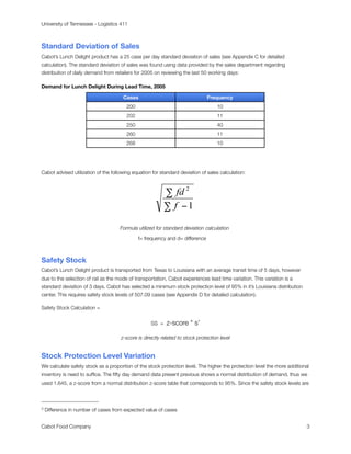
Appendix C: Standard Deviation
of Sales
Expected Value (cases) = 241 cases
Observation: Demand pattern is unstable
Assumption: When demand pattern is unstable, Weighted Moving Average is the appropriate method for calculating the
Expected Value
Instance of demand cases frequency weight ( w )
(w) • (x)
(n) (x) ( f ) ( f ÷∑ f )
1 200 10 0.12 24.39
2 202 11 0.13 27.10
3 250 40 0.49 121.95
4 260 11 0.13 34.88
5 268 10 0.12 32.68
Sum ( ∑ ) 1180 82 1.00 241.00
Expected Value = 241 cases
∑ [(Weight for instance of demand n ) ( number of cases per instance of demand n )]
∑ weights
∑ [ (.12)( 200)+(.13)(202)+(.49)(250)+(.13)(260)+(.12)(268) ]
= 241
∑ [(.12)+(.13)+(.49)+(.13)+(.12)]
Standard Deviation of Sales = 25 cases
Standard Deviation of Sales Equation:
f= frequency and d= difference
Cabot Food Company
9

12. University of Tennessee
Appendix C continued
cases frequency difference ( d )
d2 f • d2 f-1
(x) ( f ) ( EV - x )
200 10 41 1681 16,810 9
202 11 39 1521 16,731 10
EV = 241 250 40 -9 81 3240 39
260 11 -19 361 3971 10
268 10 -27 729 7290 9
Sum ( ∑ ) 48,042 77
Sum of frequency multiplied by difference squared: ∑ f • d2 = 48,042
Sum of frequency minus 1: ∑ f - 1 = 77
Standard deviation of Sales = 24.98 cases
48042
= 24.98
77
Cabot Food Company
10

13. University of Tennessee
Appendix D: Safety Stock
Safety Stock = 512 cases
Stock protection level = 95%
Corresponding z-score (Z) = 1.645
Lead Time (LT) = 5 days
Standard Deviation in Lead Time (σ(LT)) = 3 days
Standard Deviation of Sales (σ(D)) = 24.978
Variance = σ(D)2 = 623.922
Average Daily Demand (d) = 101.053
Observation: Lead time is uncertain
S’ = Square root of [ LT(σ(D)2) + d2(σ(LT)2) ]
= Square root of [ 5(623.92) + (101.05)2(3)2 ]
= Square root of [ 3,119.61 + 91904.71 ]
= Square root of [ 95,024.32 ]
= 308.26
Safety Stock =
Z * S’
1.645 * 308.26 = 507.09 cases
Cabot Food Company
11

14. University of Tennessee
Appendix E: Stock Protection
Level
Inventory and Inventory Cost variation with Change Stock Protection Levels :
S’ = 308.26
Safety Stock = Z * S’
Inventory Carrying Cost = 20%
Cost of Goods Sold = $106.88 per case
Safety Stock Cost = Inventory Carrying Cost * Cost of Goods Sold * Z * S’
Stock Protection Safety Stock Safety Stock
Z-score S’
Level (Z * S’) Cost
92% 1.405 308.26 433.11 $9,258.06
95% 1.645 308.26 507.09 $10,839.51
99% 2.326 308.26 717.01 $15,326.86
Additional inventory calculation:
Assumption: Changes in inventory levels and corresponding inventory costs effect safety stock costs singularly. The
stock protection level will not alter the order quantity.
At Stock Protection level of 99%:
Additional Inventory held = Absolute Value | 95% Safety Stock levels - 99% Safety Stock levels |
= | 507 - 717 | = 210 Cases
Additional Inventory costs = Absolute Value | 95% Safety Stock costs - 99% Safety Stock costs |
= | $10,839.51 - $15,326.86 | = $4,487.15
At Stock Protection level of 92%:
Reduction in Inventory held = Absolute Value | 95% Safety Stock levels - 92% Safety Stock levels |
= | 507 - 433 | = 74 Cases
Reduction in Inventory costs = Absolute Value | 95% Safety Stock costs - 92% Safety Stock costs |
= | $10,839.51 - $9,258.06 | = $1,581.37
Cabot Food Company
12

15. University of Tennessee
Appendix F: Reorder Point
Reorder Point Corresponding to Stock Protection Levels :
Economic Order Quantity: 307.49 cases
Safety Stock Levels (Z*S’):
At 92% Stock Protection: 433.11 cases
At 95% Stock Protection: 507.09 cases
At 99% Stock Protection: 717.01 cases
Average Daily Demand: 101.053 cases
Lead Time: 5 days
Reorder Point=
Average Daily Demand * Lead TIme (Same units as Demand) + Safety Stock
101.053 * 5 days + Safety Stock
Observation: Only Safety stock varies with Stock Protection level.
At 92% Stock Protection: 505.265 + 433.11 cases = 938.38 cases
At 95% Stock Protection: 505.265 + 507.09 cases = 1012.35 cases
At 99% Stock Protection: 505.265 + 717.01 cases = 1,222.276 cases
Cabot Food Company
13

16. University of Tennessee
Appendix G: Service Levels
Expected Service Levels :
Economic Order Quantity: 307.49 cases
Expected Z score (Ez) :
At 92% Stock Protection: .0363
At 95% Stock Protection: .0209
At 99% Stock Protection: .0035
Economic Order Quantity = 307.49
S’ = 308.26
Expected Service Level=
1- [ (S’)(Ez) ÷ Economic Order Quantity ]
At 92% Stock Protection: 1 - [ (308.26)(.0363) ÷ 307.49 ] = 96.36%
At 95% Stock Protection: 1 - [ (308.26)(.0209) ÷ 307.49 ] = 97.88%
At 99% Stock Protection: 1 - [ (308.26)(.0035) ÷ 307.49 ] = 99.66%
Stock Protection Expected Z- Expected Service
Z-score
Level Score Level
92% 1.405 0.0363 96.36%
95% 1.645 0.0209 97.88%
99% 2.326 0.0035 99.66%
Cabot Food Company
14

17. University of Tennessee
Appendix H: Total Cost
Total Inventory Cost at 95% service level = $139,713.54
Service level = 1- [ (S’)(Ez) ÷ Economic Order Quantity ]
95% service level = 1 - [ (308.26)(Ez) ÷ 307.49 ]
1 - .95 = [ (308.26)(Ez) ÷ 307.49 ]
[ (.05)(307.49) ÷ (308.26) ] = Ez
Ez = .0498
Z-Score (Z) = 1.258
Total Cost:
[ (D)(S) ÷ Q ] + (I)(C) * [ (Q ÷ 2) + (Z)(S’) ]5 + [ (k)(D)(E(z))(S’) ÷ Q ] + Outbound Transit Cost + Inbound transit cost
(D) = 25263.16 cases
(S) = $40
Economic Order Quantity (Q) = 307.49 Cases
(I) = 20%
(C) = $106.88
(Z) = 1.258
(S’) = 308.26
Stock Out Loss (K) = $90
(E(z)) = .0498
Average Daily Demand (d) = 101.05 cases
In-Transit Carrying Cost = 15%
Inbound Transit Costs: $8100
Assumption: Costs due to Lead Time Variation is accounted for in Safety Stock element of Total cost
Lead Time = 5 days
= (Average Daily demand * Lead Time) * In-transit Carrying Cost * Cost of Goods Sold
= [ (101.05 Cases * 5 days)) ] * .15 * $106.88
= $8100
Outbound Transit Cost: $3240
Lead Time = 2 days
= (Average Daily demand * Lead Time) * In-transit Carrying Cost * Cost of Goods Sold
= [ (101.05 Cases * 2 days) ] * .15 * $106.88
= $3240
5 Please note that the equation for inventory carry cost and safety stock costs have been combined in this equation
Cabot Food Company
15

18. University of Tennessee
Appendix H continued
Total Costs =
[ (D)(S) ÷ Q ] + (I)(C) * [ (Q ÷ 2) + (Z)(S’) ] + [ (k)(D)(E(z))(S’) ÷ Q ] + Outbound Transit Cost + Inbound transit cost
[ (25263.16 cases)($40) ÷ 307.49 Cases ] + (.2)($106.88) [(307.49 Cases ÷ 2) + (1.258)(308.26)]
+ [ ($90)(25263.16 cases)(.0498)(308.26) ÷ 307.49] + $3240 + $8100
= [$3286.34] + [$11,575.37] + [$113513.83] + [$3240] + [$8100] = $139,713.54
Cabot Food Company
16