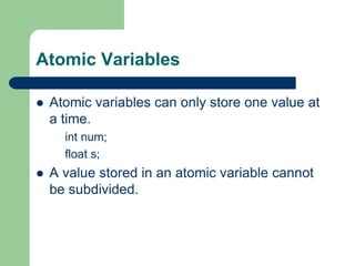
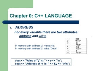
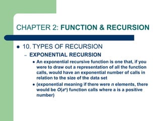
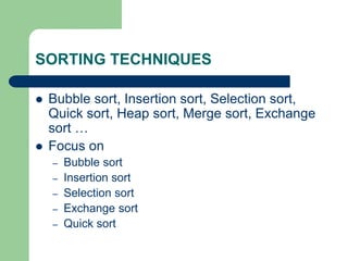
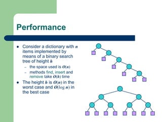
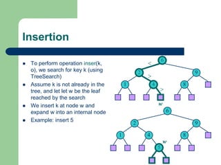
The document discusses various topics related to C++, data structures, algorithms, and functions. It covers atomic variables in C++, pointers, arrays, structures, functions, recursion, and searching techniques. It also discusses complexity of algorithms. Some key topics include linear and binary search, recursion types like linear, tail, and mutual recursion, and analyzing complexity of algorithms.
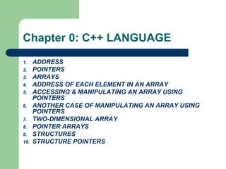
![Chapter 0: C++ LANGUAGE
3. ARRAYS
1. An array is a data structure
2. used to process multiple elements with the same data
type when a number of such elements are known.
3. An array is a composite data structure; that means it
had to be constructed from basic data types such as
array integers.
1. int a[5];
2. for(int i = 0;i<5;i++)
1. {a[i]=i; }](https://image.slidesharecdn.com/canddatastructure-230708134332-7c86588a/85/C-and-Data-Structure-ppt-8-320.jpg)
![Chapter 0: C++ LANGUAGE
4. ADDRESS OF EACH ELEMENT IN AN
ARRAY
Each element of the array has a memory
address.
void printdetail(int a[])
{
for(int i = 0;i<5;i++)
{
cout<< "value in array “<< a[i] <<“ at address: “ << &a[i]);
}](https://image.slidesharecdn.com/canddatastructure-230708134332-7c86588a/85/C-and-Data-Structure-ppt-9-320.jpg)
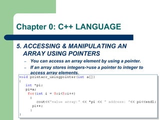
![Chapter 0: C++ LANGUAGE
6. ANOTHER CASE OF MANIPULATING AN
ARRAY USING POINTERS
The array limit is a pointer constant : cannot
change its value in the program.
int a[5]; int *b;
a=b; //error
b=a; //OK
It works correctly even using
a++ ???](https://image.slidesharecdn.com/canddatastructure-230708134332-7c86588a/85/C-and-Data-Structure-ppt-11-320.jpg)
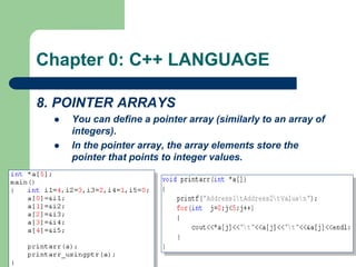
![Chapter 0: C++ LANGUAGE
7. TWO-DIMENSIONAL ARRAY
int a[3][2];](https://image.slidesharecdn.com/canddatastructure-230708134332-7c86588a/85/C-and-Data-Structure-ppt-12-320.jpg)
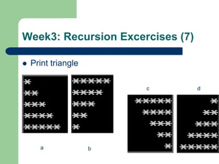
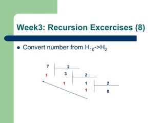
![Week3: Recursion Excercises (5)
E4. Write a recursion function to calculate:
– S=a[0]+a[1]+…a[n-1]
A: array of integer numbers](https://image.slidesharecdn.com/canddatastructure-230708134332-7c86588a/85/C-and-Data-Structure-ppt-47-320.jpg)
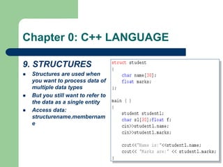
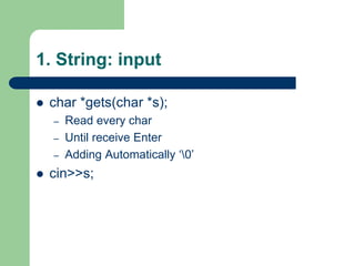
![1. String: structure
String
– is array of char
– Ending with null char 0 (size +1)
– Example: store 10 chars:
char str[11];
– “Example”: string const. C/C++ add 0
automayically](https://image.slidesharecdn.com/canddatastructure-230708134332-7c86588a/85/C-and-Data-Structure-ppt-52-320.jpg)
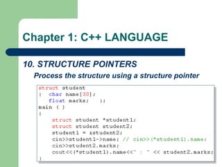
![1. String: declare
Declare string
– Using array of chars
char str[] = {‘H’,’e’,’l’,’l’,’o’,’0’}; //declare with null
char str[] = “Hello”; //needn’t null
– Using char pointer
char *str = “Hello”;](https://image.slidesharecdn.com/canddatastructure-230708134332-7c86588a/85/C-and-Data-Structure-ppt-53-320.jpg)

![1. String: Problem with buffer?
Keyboard buffer
char szKey[] = "aaa";
char s[10];
do {
cout<<"doan lai di?";
gets(s);
} while (strcmp (szKey,s) != 0);
puts ("OK. corect");
If user input: aaaaaaaaaaaaa???](https://image.slidesharecdn.com/canddatastructure-230708134332-7c86588a/85/C-and-Data-Structure-ppt-56-320.jpg)
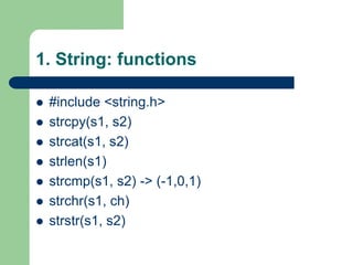
![1. String: function examples
char s1[80], s2[80];
cout << "Input the first string: :";
gets(s1);
cout << "Input the second string: ";
gets(s2);
cout << "Length of s1= " << strlen(s1);
cout << "Length of s2= " << strlen(s2);
if(!strcmp(s1, s2))
cout << "These strings are equaln";
strcat(s1, s2);
cout << "s1 + s2: " << s1 << endl;;
strcpy(s1, "This is a test.n");
cout << s1;
if(strchr(s1, 'e')) cout << "e is in " << s1;
if(strstr(s2, "hi")) cout << "found hi in " <<s2;](https://image.slidesharecdn.com/canddatastructure-230708134332-7c86588a/85/C-and-Data-Structure-ppt-58-320.jpg)
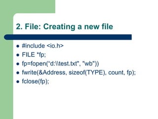
![2.File: Creating a new file
int Arr[3]
Arr
Fwrite(Arr, sizeof(int), 1, fp);
fwrite(Arr, sizeof(Arr), 1, fp);
Fwrite(&Arr[i], sizeof(int), 1, fp);
for (i=0;i<=3;i++)](https://image.slidesharecdn.com/canddatastructure-230708134332-7c86588a/85/C-and-Data-Structure-ppt-60-320.jpg)
![1. LINEAR (SEQUENTIAL) SEARCH
void lsearch(int list[],int n,int element)
{ int i, flag = 0;
for(i=0;i<n;i++)
if( list[i] == element)
{ cout<<“found at position”<<i);
flag =1;
break; }
if( flag == 0)
cout<<“ not found”;
}
flag: what for???](https://image.slidesharecdn.com/canddatastructure-230708134332-7c86588a/85/C-and-Data-Structure-ppt-70-320.jpg)
![1. LINEAR (SEQUENTIAL) SEARCH
int lsearch(int list[],int n,int element)
{ int i, find= -1;
for(i=0;i<n;i++)
if( list[i] == element)
{find =i;
break;}
return find;
}
Another way using flag
average time: O(n)](https://image.slidesharecdn.com/canddatastructure-230708134332-7c86588a/85/C-and-Data-Structure-ppt-71-320.jpg)
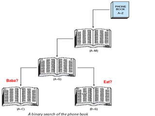
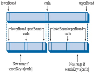
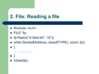
![void bsearch(int list[],int n,int element)
{
int l,u,m, flag = 0;
l = 0; u = n-1;
while(l <= u)
{ m = (l+u)/2;
if( list[m] == element)
{cout<<"found:"<<m;
flag =1;
break;}
else
if(list[m] < element)
l = m+1;
else
u = m-1;
}
if( flag == 0)
cout<<"not found";
}
average time: O(log2n)](https://image.slidesharecdn.com/canddatastructure-230708134332-7c86588a/85/C-and-Data-Structure-ppt-75-320.jpg)
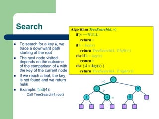
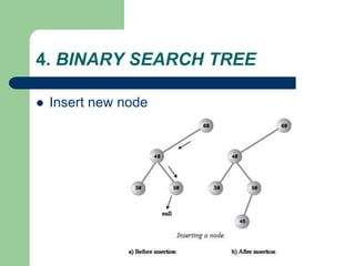
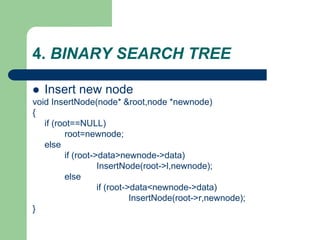
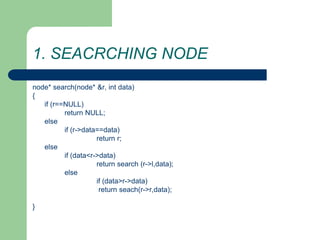
![BINARY SEARCH: Recursion
int Search (int list[], int key, int left, int right)
{
if (left <= right) {
int middle = (left + right)/2;
if (key == list[middle])
return middle;
else if (key < list[middle])
return Search(list,key,left,middle-1);
else return Search(list,key,middle+1,right);
}
return -1;
}](https://image.slidesharecdn.com/canddatastructure-230708134332-7c86588a/85/C-and-Data-Structure-ppt-76-320.jpg)
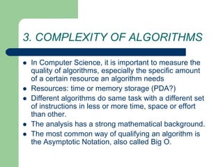
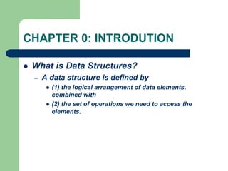
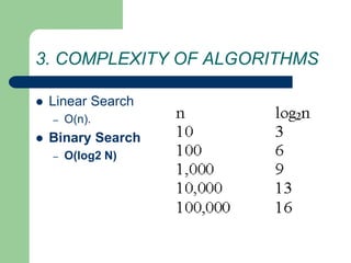
![3. COMPLEXITY OF ALGORITHMS
Example1: complexity of an algorithm
void f ( int a[], int n )
{
int i;
cout<< "N = “<< n;
for ( i = 0; i < n; i++ )
cout<<a[i];
printf ( "n" );
}
?
?
2 * O(1) + O(N)
O(N)](https://image.slidesharecdn.com/canddatastructure-230708134332-7c86588a/85/C-and-Data-Structure-ppt-79-320.jpg)
![3. COMPLEXITY OF ALGORITHMS
Example2: complexity of an algorithm
void f ( int a[], int n )
{ int i;
cout<< "N = “<< n;
for ( i = 0; i < n; i++ )
for (int j=0;j<n;j++)
cout<<a[i]<<a[j];
for ( i = 0; i < n; i++ )
cout<<a[i];
printf ( "n" );
}
?
?
2 * O(1) + O(N)+O(N2)
O(N2)](https://image.slidesharecdn.com/canddatastructure-230708134332-7c86588a/85/C-and-Data-Structure-ppt-80-320.jpg)
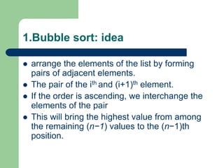
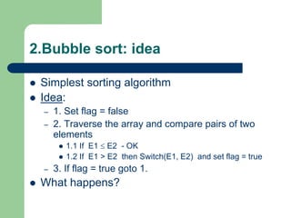
![1.Bubble sort:algorithm idea
void bubbleSort (Array S, length n) {
boolean isSorted = false;
while(!isSorted)
{
isSorted = true;
for(i = 0; i<n; i++)
if(S[i] > S[i+1])
{
swap(S[i],S[i+1];)
isSorted = false;
}
}](https://image.slidesharecdn.com/canddatastructure-230708134332-7c86588a/85/C-and-Data-Structure-ppt-90-320.jpg)
![1.Bubble sort: implement
void bsort(int list[], int n)
{
int count,j;
for(count=0;count<n-1;count++)
for(j=0;j<n-1-count;j++)
if(list[j] > list[j+1])
swap(list[j],list[j+1]);
}](https://image.slidesharecdn.com/canddatastructure-230708134332-7c86588a/85/C-and-Data-Structure-ppt-91-320.jpg)
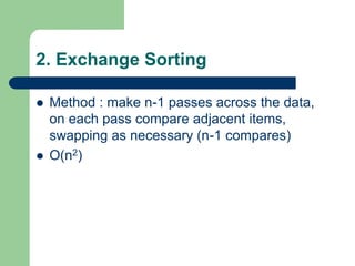
![2. Exchange Sorting
void Exchange_sort(int arr[], int n)
{
int i,j;
for(i=0;i<n-1;i++)
for(j=i+1;j<n;j++)
if(arr[i] > arr[j])
swap(arr[i],arr[j]);
}](https://image.slidesharecdn.com/canddatastructure-230708134332-7c86588a/85/C-and-Data-Structure-ppt-93-320.jpg)
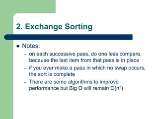
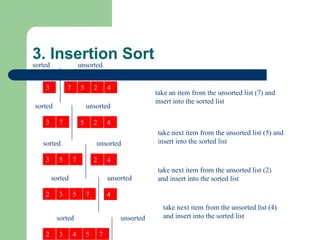
![3. Insertion Sort
void insertionSort(int arr[], int n){
int j, key;
for(int i = 1; i < n; i++){
key = arr[i];
j = i - 1;
while(j >= 0 && arr[j] > key)
{ arr[j + 1] = arr[j];
j = j - 1;
}
arr[j + 1] = key;
}
}](https://image.slidesharecdn.com/canddatastructure-230708134332-7c86588a/85/C-and-Data-Structure-ppt-97-320.jpg)
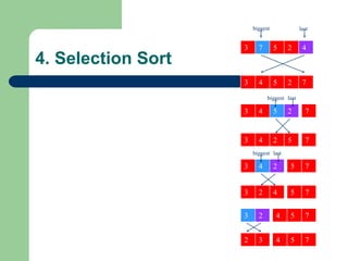
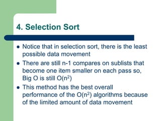
![4. Selection Sort
void selection_sort(int arr[], int n)
{int i, j, min;
for (i = 0; i < n - 1; i++)
{
min = i;
for (j = i+1; j < n; j++)
{ if (list[j] < list[min]) min = j; }
swap(arr[i],arr[min]);
}
}](https://image.slidesharecdn.com/canddatastructure-230708134332-7c86588a/85/C-and-Data-Structure-ppt-101-320.jpg)
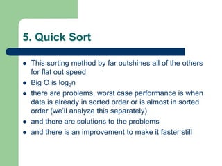
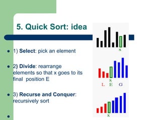
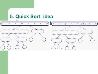
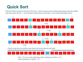
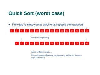
![Quick Sort
void quickSort(int Arr[], int lower, int upper)
{
int x = Arr[(lower + upper) / 2];
int i = lower; int j = upper;
do{
while(Arr[i] < x) i ++;
while (Arr[j] > x) j --;
if (i <= j)
{
swap(Arr[i], Arr[j]);
i ++; j --; }
}while(i <= j);
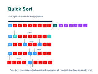
if (j > lower)
quickSort(Arr, lower, j);
if (i < upper)
quickSort(Arr, i, upper);
}](https://image.slidesharecdn.com/canddatastructure-230708134332-7c86588a/85/C-and-Data-Structure-ppt-111-320.jpg)
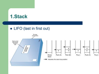
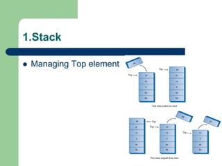
![1.Stack: implement using array
#define MAX 10
void main()
{
int stack[MAX];
int top = -1;
push(stack,top, 10 );
pop(stack,top,value);
int value;
cout<<value;
}](https://image.slidesharecdn.com/canddatastructure-230708134332-7c86588a/85/C-and-Data-Structure-ppt-115-320.jpg)
![1.Stack: implement using array
void push(int stack[], int &top, int value)
{
if(top < MAX )
{
top = top + 1;
stack[top] = value;
}
else
cout<<"The stack is full";
}](https://image.slidesharecdn.com/canddatastructure-230708134332-7c86588a/85/C-and-Data-Structure-ppt-116-320.jpg)
![1.Stack: implement using array
void pop(int stack[], int &top, int &value)
{
if(top >= 0 )
{
value = stack[top];
top = top - 1;
}
else
cout<<"The stack is empty ";
}](https://image.slidesharecdn.com/canddatastructure-230708134332-7c86588a/85/C-and-Data-Structure-ppt-117-320.jpg)
![2.QUEUE: implement using array
#define MAX 10
void main()
{
int queue[MAX];
int bottom,top,count=0;
bottom=top=-1;
enqueue(queue,count,top, 100 );
int value;
dequeue(queue,count,bottom,top,value);
}](https://image.slidesharecdn.com/canddatastructure-230708134332-7c86588a/85/C-and-Data-Structure-ppt-120-320.jpg)
![2.QUEUE: implement using array
void enqueue(int queue[],int &count, int &top, int value)
{
if(count< MAX)
{
count++;
top= (top +1)%MAX;
queue[top] = value;
}
else
cout<<"The queue is full";
}](https://image.slidesharecdn.com/canddatastructure-230708134332-7c86588a/85/C-and-Data-Structure-ppt-121-320.jpg)
![2.QUEUE: implement using array
void dequeue(int queue[], int &count,int &bottom,int top, int
&value)
{
if(count==0)
{
cout<<"The queue is empty";
exit(0);
}
bottom = (bottom + 1)%MAX;
value = queue[bottom];
count--;
}](https://image.slidesharecdn.com/canddatastructure-230708134332-7c86588a/85/C-and-Data-Structure-ppt-122-320.jpg)


![Getting Started with Apache Spark: Big Data Made Simple [Free Meetup]](https://cdn.slidesharecdn.com/ss_thumbnails/apachesparkgettingstarted-260203175547-8361bcc3-thumbnail.jpg?width=640&height=640&fit=bounds)


