This document provides a summary of a design manual for steel-to-concrete joints. It describes a component method for modeling such joints using individual resistance, stiffness, and deformation components for both the concrete and steel parts. These include components for headed studs, stirrups, concrete breakout, pullout, bending plates, reinforcement bars, and slip. The document outlines how to combine the behavior of these components to determine the overall joint resistance, stiffness, and failure load considering forces like tension, shear, bending and interaction effects. It also provides simplified approaches based on technical specifications. Worked examples are given to demonstrate applying the theory to design pinned and moment resistant base plates and beam-to-column connections.


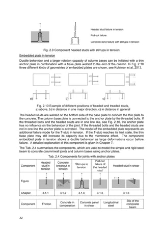
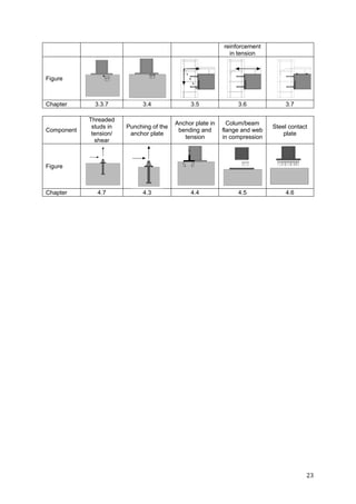

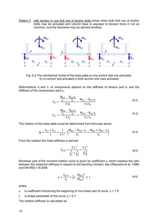
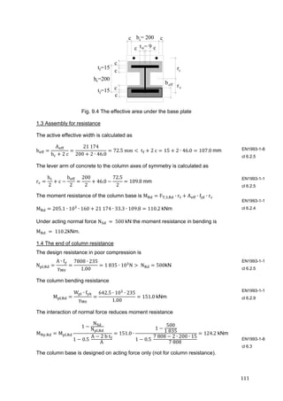
![25
δ ,
N , L
A , E
σ , L
E
[mm] (3.1)
where
Lh is length of the anchor shaft [mm]
NRd,s is design tension resistance of the headed stud [N]
Es is elastic modulus of the steel, Es 210 000 N/mm² [N/mm²]
As,nom is nominal cross section area of all shafts
A ,
d ,
4
mm² (3.2)
where
ds,nom is nominal diameter of the shaft [mm]
The design load at steel yielding failure is calculated as given below
N , A ,
f
γ
n π
d ,
4
f
γ
N (3.3)
where
fuk is characteristic ultimate strength of the shaft material of the headed stud [N/mm²]
n is number of headed studs in tension [-]
Ms is partial safety factor for steel [-]
Exceeding the design steel yielding strength fyd, the elongation will strongly increase without
a significant increase in load up to a design strain limit su. For the design, this increase of
strength is neglected on the safe side and the stiffness is assumed to be zero, ks 0 N/mm.
Depending on the product the failure shall be assumed at the yielding point. In general,
fasteners as headed studs are deemed to have an elongation capacity of at least su 0.8 %.
This limit shall be used to determine the response of the fasteners unless it is proven by means
of tests that they have a higher elongation capacity.
Therefore the stiffness ks is described as given below depending on the displacement or load
k
A , E
L
for N N , N/mm (3.4)
k 0 for δ δ , e and N N , N/mm (3.5)
where
δRd,sy is displacement at yielding of the shaft, see Eq. (3.1) [mm]
εsu is maximum elongation capacity of the shaft, 0.8 % [-]
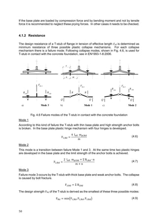
3.1.2 Headed studs in tension, component CC
The component concrete breakout in tension is described using the design load NRd,c for
concrete cone failure and the displacement in the softening branch after failure. Up to the
design load the component can´t be assumed as absolutely rigid without any displacement.
The displacement corresponding to design load is given by](https://image.slidesharecdn.com/boltdesign-manualiien-191004025827/85/Bolt-design-manual-ii-en-26-320.jpg)
![26
δ ,
N ,
k ,
[mm] (3.6)
The design load at concrete cone failure is calculated as
N , N , ψ , ψ ,
ψ ,
γ
[N] (3.7)
where
N , is characteristic resistance of a single anchor without edge and spacing effects
N , k h .
f .
[N] (3.8)
where
k1 is basic factor 8.9 for cracked concrete and 12.7 for non-cracked concrete [-]
hef is embedment depth given according to the product specifications [mm]
fck is characteristic concrete strength according to EN206-1:2000 [N/mm²]
ψ , is factor accounting for the geometric effects of spacing and edge distance [-]
ψ ,
,
,
[-] (3.9)
where
ψ , is factor accounting for the influence of edges of the concrete member on the
distribution of stresses in the concrete
ψ , 0.7 0.3
c
c ,
1 (3.10)
where
ψ , is factor accounting for the negative effect of closely spaced reinforcement in the
concrete member on the strength of anchors with an embedment depth hef 100 mm
0.5 hef / 200 for s 150 mm (for any diameter) [-]
or s 100 mm (for ds 10 mm)
1.0 for s 150 mm (for any diameter) [-]
γMc is 1.5 for concrete [-]
A , is reference area of the concrete cone of an individual anchor with large spacing and
edge distance projected on the concrete surface [mm²]. The concrete cone is idealized
as a pyramid with a height equal to hef and a base length equal to scr,N with
s , 3.0 h [mm] (3.11)
c , 0.5 s , 1.5 h [mm] (3.12)
where
Ac,N is actual projected area of concrete cone of the anchorage at the concrete surface,
limited by overlapping concrete cones of adjacent anchors, s scr,N, as well as by edges
of the concrete member, c ccr,N. It may be deduced from the idealized failure cones
of single anchors [mm²]
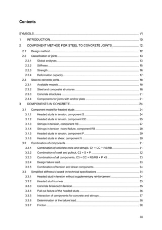
To avoid a local blow out failure the edge distance shall be larger than 0.5 hef. Due to sudden
and brittle failure, the initial stiffness for concrete cone is considered as infinity, i.e. till the actual
load, Nact is less than or equal to the design tension resistance for concrete cone, the](https://image.slidesharecdn.com/boltdesign-manualiien-191004025827/85/Bolt-design-manual-ii-en-27-320.jpg)
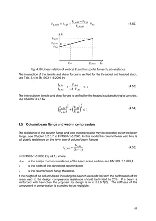
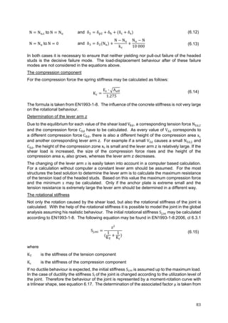
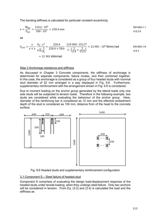
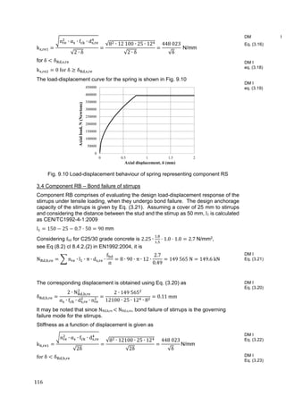
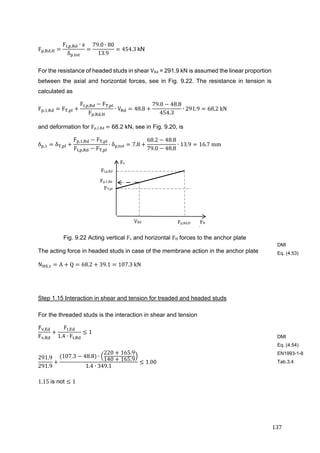
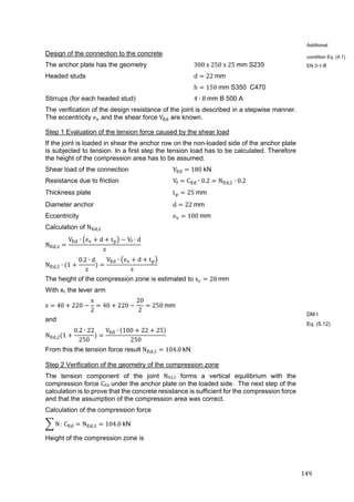
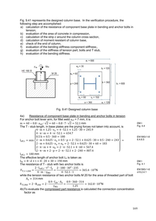
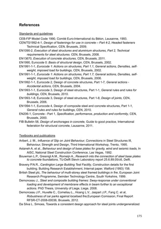
![27
displacement c is zero. Once the design load is exceeded, the displacement increases with
decreasing load, descending branch. Thus, the load-displacement behaviour in case of
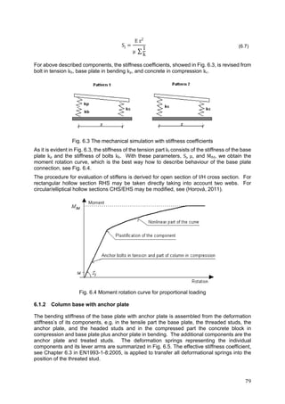
concrete cone breakout is idealized as shown in Fig. 3.2.
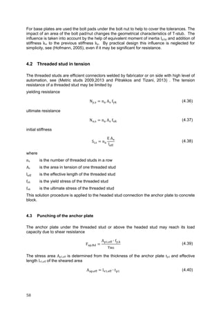
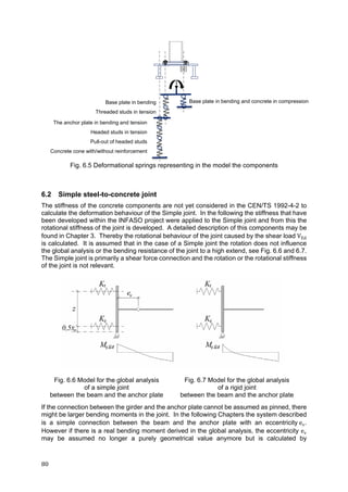
Fig. 3.2 Idealized load-displacement relationship for concrete cone breakout in tension
The stiffness of the descending branch kc,de for the design is described with the following
function
k , α f h ψ , ψ , ψ , [N/mm] (3.13)
where
αc is factor of component concrete break out in tension, currently αc ‐537
hef is embedment depth of the anchorage [mm]
fck is characteristic concrete compressive strength [N/mm²]
Ac,N is projected surface of the concrete cone [mm2]
A , projected surface of the concrete cone of a single anchorage [mm2]
The displacement δc as a function of the acting load Nact is described using the design
resistance and the stiffness of the descending branch.
For ascending part
N N , and δc 0 (3.14)
For descending branch
δ 0 mm and δ
N N ,
k ,
(3.15)
3.1.3 Stirrups in tension, component RS
The component stirrups in tension was developed based on empirical studies. Therefore the
tests results were evaluated to determine the displacement of the stirrups depending on the
load Nact acting on the stirrup. The displacement is determined like given in the following
equation
δ , ,
2 N , ,
α f d , n
[mm] (3.16)
where
Nact
NRd,c
kc,de
δc
1](https://image.slidesharecdn.com/boltdesign-manualiien-191004025827/85/Bolt-design-manual-ii-en-28-320.jpg)
![28
αs is factor of the component stirrups, currently αs 12 100 [-]
NRd,s,re is design tension resistance of the stirrups for tension failure [N]
ds,re is nominal diameter of thereinforcement leg [mm]
fck is characteristic concrete compressive strength [N/mm²]
nre is total number of legs of stirrups [-]
The design load for yielding of the stirrups is determined as given
N , , A , f , n π
d ,
4
f , [N] (3.17)
where
As,re is nominal cross section area of all legs of the stirrups [mm²]
ds,re is nominal diameter of the stirrups [mm]
fyd is design yield strength of the shaft material of the headed stud [N/mm²]
nre is total number of legs of stirrups [-]
Exceeding the design steel yielding strength fyd,re the elongation will increase with no significant
increase of the load up to a strain limit εsu,re of the stirrups. For the design this increase of
strength is neglected on the safe side. In general reinforcement steel stirrups shall have an
elongation capacity of at least εsu,re = 2,5 %. So the design strain limit εsu,re is assumed to be
2.5 %. The displacement as a function of the acting load is determined as
k ,
n α f d ,
√2 δ
for δ δ , , [N/mm]
(3.18)
k , 0 for δ δ , , ε , [N/mm] (3.19)
3.1.4 Stirrups in tension - bond failure, component RB
The displacement of the concrete component stirrups in tension is determined under the
assumption that bond failure of the stirrups will occur. This displacement is calculated with
equation (3.19) as
δ , ,
2 N , ,
α f d , n
[mm] (3.20)
where
αs is factor of the component stirrups, currently αs 12 100 [-]
NRd,b,re is design tension resistance of the stirrups for bond failure [N]
ds,re is nominal diameter of the stirrups [mm]
fck is characteristic concrete compressive strength [N/mm²]
The design anchorage capacity of the stirrups according CEN/TS-model [5] is determined the
design tension resistance of the stirrups for bond failure
N , , n ,
l π d , f
α
[N] (3.21)
where
ns,re is number of legs [-]](https://image.slidesharecdn.com/boltdesign-manualiien-191004025827/85/Bolt-design-manual-ii-en-29-320.jpg)
![29
l1 is anchorage length [mm]
ds,re is nominal diameter of the stirrups [mm]
fbd is design bond strength according to EN1992-1-1:2004 [N/mm²]
α is factor according to EN1992-1-1:2004 for hook effect and large concrete cover,
currently 0.7 · 0.7 = 0.49 [-]
k ,
n α f d ,
√2 δ
for δ δ , , [N/mm]
(3.22)
k , 0 for δ δ , , ε , [N/mm] (3.23)
3.1.5 Headed studs in tension, component P
The pull out failure of the headed studs will take place if the local stresses at the head are
larger than the local design resistance. Up to this level the displacement of the headed stud
will increase due to the increasing pressure under the head.
δ , , k ∙
N ,
A ∙ f ∙ n
[mm] (3.24)
δ , , 2 k ∙
min N , ; N ,
A ∙ f ∙ n
δ , , [mm] (3.25)
k α ∙
k ∙ k
k
(3.26)
where
Ah is area on the head of the headed stud [mm²]
A
π
4
∙ d d (3.27)
where
ka is form factor at porous edge sections [-]
k 5/a 1 (3.28)
where
ap is factor considering the shoulder width [mm]
a 0.5 ∙ d d (3.29)
where
kA is factor considering the cross section depending on factor ka [-]
k 0.5 ∙ d m ∙ d d 0.5 ∙ d (3.30)
where
n is number of the headed studs [-]](https://image.slidesharecdn.com/boltdesign-manualiien-191004025827/85/Bolt-design-manual-ii-en-30-320.jpg)
![30
αp is factor of the component head pressing, currently is αp 0.25 [-]
k2 is factor for the headed studs in non-cracked concrete, currently 600 [-]
is factor for the headed studs in cracked concrete, currently 300 [-]
m is pressing relation, m 9 for headed studs [-]
dh is diameter of the head [mm]
ds is diameter of the shaft [mm]
NRd,p is design load at failure in cases of pull out
N , n p A /γ (3.31)
where
puk is characteristic ultimate bearing pressure at the headed of stud [N/mm2]
NRd,c is design load for concrete cone failure without supplementary reinforcement
N , N , ψ , ψ ,
ψ ,
γ
[N] (3.32)
where
NRd,re design load at failure of the supplementary reinforcement minimum value of
N , , A , f , n π ,
f , and N , , ∑
∙ ∙ , ∙
,
[N] (3.33)
The stiffness as a function of the displacement is determined as
k ,
A f n
δ k
[N/mm] (3.34)
k ,
A f n δ δ ,
2 δ k
[N/mm] (3.35)
k , min N , ; N , /δ k , 1 δ , , /δ [N/mm] (3.36)
The stiffness kp,de depends on the failure modes. If the supplementary reinforcement fails by
yielding (NRd,s,re NRd,b,re and NRd,s,re NRd,p) the design stiffness kp,de is assumed as 104 N/mm²,
negative due to descending branch.
In all other cases (e.g. NRd,s,re NRd,b,re or NRd,s,re NRd,p) kp,de shall be assumed as infinite due to
brittle failure. The stiffness in case of pull out failure is calculated using the minimum value of
the stiffness’s calculated with equation (3.34) to (3.36).
k , min k , ; k , ; k , [N/mm] (3.37)
3.1.6 Headed studs in shear, component V
The load-displacement behaviour mainly depends on the pressure to the concrete near the
surface of the concrete member. Due to concrete crushing at the surface of the concrete
member, the displacement under shear loading varies very large with a coefficient of variation
about 40 % to 50 %. However a semi-empirical calculation shows that the displacement at
failure mainly depends on the acting loading, the diameter of the anchors and the embedment](https://image.slidesharecdn.com/boltdesign-manualiien-191004025827/85/Bolt-design-manual-ii-en-31-320.jpg)
![31
depth. Therefore the displacement under shear loading for a given load level is calculated,
see (Hofmann 2005), using the following equation only as an estimation
δ , k
V
d
h .
[mm] (3.38)
where
kv empirical value depending on the type of anchor [-], for headed studs kv 2 to 4
VRd design failure load as the minimum of the design failure loads calculated for the different
failure modes (VRd,s, VRd,cp, VRd,c , VRd,p) given according to the technical product
specification CEN/TS 1992-4-1 or (FIB Bulletin 58, 2011)
The displacement at ultimate load up three times larger than the displacement at the design
load level due to the assumption, that the concrete near the surface is not fully crushed at
design load level.
3.2 Combination of components
To come up with the total stiffness of the connection with headed studs anchored in concrete
with or without supplementary reinforcement, the stiffness’s must be combined. The
combination depends on whether the components are acting in parallel, equal displacements,
or in serial, equal load. Three combinations are given, see (Hofmann, 2005):
Combination C1
Concrete cone failure with or without supplementary reinforcement, ks,re = 0 and kb,re = 0
Combination C2
Displacement due to steel elongation and head pressure, pull out
Combination C3
Total connection of headed studs anchored in concrete with supplementary reinforcement
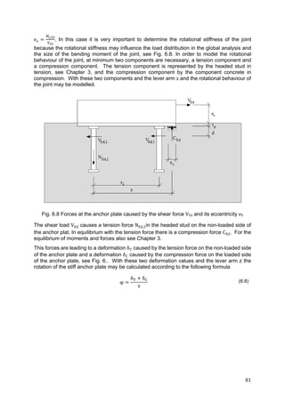
Fig. 3.3 Combinations of different single components
for an anchorage with supplementary reinforcement
3.2.1 Combination of concrete cone and stirrups, C1 = CC + RS/RB
If both components are summarized, the load is calculated using the sum of the loads at the
same displacement due to the combination of the components using a parallel connection](https://image.slidesharecdn.com/boltdesign-manualiien-191004025827/85/Bolt-design-manual-ii-en-32-320.jpg)
![32
from the rheological view. Two ranges must be considered. The first range is up to the load
level at concrete failure NRd,c the second up to a load level of failure of the stirrups NRd,s,re or
NRd,b,re.
k . k k , ∞ for N N , [N/mm] (3.39)
This leads to the following equation
k .
n α f d ,
√2 δ
for N N , [N/mm]
(3.40)
In the second range the load is transferred to the stirrups and the stiffness decreases. The
stiffness is calculated if Nact is larger than NRd,c with the following equation
k . k k , for N N , [N/mm] (3.41)
This leads to a relative complex equation
k .
N ,
δ
k , k ,
δ ,
δ
n α f d ,
√2 δ (3.42)
for N N , , N , , [N/mm]
If the load exceeds the ultimate load given by NRd,s,re or NRd,b,re the stiffness of the stirrups are
negligible. Therefore the following equation applies:
k . k k , 0 for N N , , N , , [N/mm] (3.43)
3.2.2 Combination of steel and pullout, C2 = S + P
If both components are summarized the load is calculated using the sum of the displacements
at the same load Nact due to the combination of the components using a serial connection from
the rheological view. This is done by summing up the stiffness’s as given below
k
1
k
1
k
[N/mm] (3.44)
This loads to the following equation
k
L
A , E
1
k
L
A , E
1
min k ; k ; k
[N/mm] (3.45)
where
kp is the minimum stiffness in case of pullout failure as the minimum of kp1, kp2 and kp3](https://image.slidesharecdn.com/boltdesign-manualiien-191004025827/85/Bolt-design-manual-ii-en-33-320.jpg)
![33
3.2.3 Combination of all components, C3 = CC + RS/RB + P +S
To model the whole load- displacement curve of a headed stud embedded in concrete with a
supplementary reinforcement the following components are combined:
concrete and stirrups in tension, components CC and RB/RS, as combination C1,
shaft of headed stud in tension, component S, and
pull-out failure of the headed stud component P as Combination 2.
The combinations C1 and C2 is added by building the sum of displacements. This is due to
the serial function of both components. That means that these components are loaded with
the same load but the response concerning the displacement is different. The combination of
the components using a serial connection leads to the following stiffness of the whole
anchorage in tension:
1/k 1/k 1/k [N/mm] (3.46)
where
kC1 is the stiffness due to the displacement of the anchorage in case of concrete cone
failure with supplementary reinforcement, see combination C1 [N/mm], if no
supplementary reinforcement is provided kC1 is equal to kc
kC2 is the stiffness due to the displacement of the head, due to the pressure under the head
on the concrete, and steel elongation, see combination C2 [N/mm]
3.2.4 Design failure load
In principle two failure modes are possible to determine the design failure load NRd,C3 for the
combined model. These modes are failure of
the concrete strut NRd,cs,
the supplementary reinforcement NRd,re.
The design failure load in cases of concrete strut failure is calculated using the design load in
case of concrete cone failure and an increasing factor to consider the support of the
supplementary reinforcement, angle of the concrete strut,
N , ψ N , N (3.47)
where
NRd,c is design failure load in case of concrete cone failure, see Eq. 3.7 [N]
Ψsupport is support factor considering the confinement of the stirrups
2.5
x
h
1 (3.48)
where
x is distance between the anchor and the crack on the concrete surface assuming a crack
propagation from the stirrup of the supplementary reinforcement to the concrete surface
with an angle of 35° [mm]](https://image.slidesharecdn.com/boltdesign-manualiien-191004025827/85/Bolt-design-manual-ii-en-34-320.jpg)
![34
Fig. 3.4 Distance between the anchor and the crack on the concrete surface
The load is transferred to the stirrups and the concrete cone failure load is reached. Depending
on the amount of supplementary reinforcement the failure of the stirrups can decisive
NRd,re NRd,cs. Two failure modes are possible:
steel yielding of stirrups NRd,s,re, see equation (3.16),
anchorage failure of stirrups NRd,b,re, see equation (3.20).
The corresponding failure load is calculated according to equation (3.49) summarizing the
loads of the corresponding components
N , min N , , ; N , , N , δ ∙ k , [N] (3.49)
where
NRd,c is design failure load in case of concrete cone failure, see equation (3.7), [N]
NRd,s,re is design failure load in case of yielding of the stirrups of the supplementary
reinforcement, see equation (3.16) [N]
NRd,b,re is design failure load in case of bond failure of the stirrups of the supplementary
reinforcement, see equation (3.20) [N]
kc,de is stiffness of the concrete cone in the descending branch, see equation (3.13) [N/mm]
δf is corresponding displacement at failure load NRd,s,re or NRd,b,re [mm]
3.2.5 Combination of tension and shear components
The displacements in tension and shear is calculated by the sum of the displacement vectors.
3.3 Simplified stiffness’s based on technical specifications
3.3.1 Headed stud in tension without supplementary reinforcement
For simplification the displacements and the stiffness of headed studs or anchorages is
estimated using technical product specifications. The elongation δRd is estimated up to the
design load NRd using the displacements given in the technical product specification. The
displacement is estimated by the following equation
δ ,
δ ,
N
N (3.50)
where
δN,ETA is displacement given in the product specifications for a corresponding load
NETA is tension load for which the displacements are derived in the product specifications](https://image.slidesharecdn.com/boltdesign-manualiien-191004025827/85/Bolt-design-manual-ii-en-35-320.jpg)
![35
NRd is design tension resistance
The stiffness of the anchorage is calculated with the following equation
k ,
δ ,
N
(3.51)
where
δN,ETA is displacement given in the product specifications for a corresponding load
NETA is tension load for which the displacements are derived in the product specifications
3.3.2 Headed stud in shear
For the design the displacement δv is estimated up to the design load VRd using the
displacements given in the technical product specification. The displacement is estimated
using the displacements far from the edge δv,ETA for short term and long term loading. The
displacement is estimated by the following equation
δ ,
δ ,
V
V (3.52)
where
δV,ETA is displacement given in the product specifications for a corresponding load
VETA is shear load for which the displacements are derived in the product specifications
VRd,c is design shear resistance
The stiffness of the anchorage is calculated with the following equation
k ,
δ ,
V
(3.53)
where
δV,ETA is displacement given in the product specifications for a corresponding load
VETA is shear load for which the displacements are derived in the product specifications
3.3.3 Concrete breakout in tension
The characteristic load corresponding to the concrete cone breakout in tension for a single
headed stud without edge influence is given by equation
N , k h .
f (3.54)
where
k1 is basic factor for concrete cone breakout, which is equal to 8.9 for cracked concrete
and 12.7 for non-cracked concrete, for headed studs, [-]
hef is effective embedment depth given according to the product specifications [mm] [-]
fck is characteristic concrete strength according to EN206-1:2000 [N/mm²]
The design load for concrete cone breakout for a single anchor, N , is obtained by applying
partial safety factor of concrete γ to the characteristic load as](https://image.slidesharecdn.com/boltdesign-manualiien-191004025827/85/Bolt-design-manual-ii-en-36-320.jpg)
![36
N ,
N ,
γ
(3.55)
For concrete, the recommended value of is γ = 1.5.
For a group of anchors, the design resistance corresponding to concrete cone breakout is
given by equation (3.56), which is essentially same as equation (3.7)
N , N , ψ , ψ , ψ , /γ (3.56)
where
N , is characteristic resistance of a single anchor without edge and spacing effects
ψ , is factor accounting for the geometric effects of spacing and edge distance
given as ψ , ,
,
A , is reference area of the concrete cone for a single anchor with large spacing and
edge distance projected on the concrete surface [mm²].
The concrete cone is idealized as a pyramid with a height equal to hef and a base
length equal to scr,N with s , 3.0 h , thus A , 9 h .
A , is reference area of the concrete cone of an individual anchor with large spacing and
edge distance projected on the concrete surface [mm²].
The concrete cone is idealized as a pyramid with a height equal to hef and a base
length equal to scr,N with s , 3,0 h mm
Ac,N is actual projected area of concrete cone of the anchorage at the concrete surface,
limited by overlapping concrete cones of adjacent anchors s scr,N,
as well as by edges of the concrete member c ccr,N.
It may be deduced from the idealized failure cones of single anchors [mm²]
c is minimum edge distance c 1.5 hef [mm]
ccr,N is critical edge distance ccr,N 1.5 hef [mm]
ψre,N is factor accounting for the negative effect of closely spaced reinforcement in the
concrete member on the strength of anchors with an embedment depth hef < 100 mm
0.5 + hef / 200 for s 150 mm, for any diameter [-]
or s < 100 mm, for ds ≤ 10 mm
1.0 for s 150 mm (for any diameter) [-]
γMc is 1.5 for concrete [-]
3.3.4 Pull out failure of the headed studs
The design load corresponding to the pull out failure of the headed stud, NRd,p is given by
N , p A /γ (3.57)
where
puk is characteristic ultimate bearing pressure at the head of stud [N/mm2]
Ah is area on the head of the headed stud [mm²]
A
π
4
∙ d d (3.57b)
dh is diameter of the head [mm]
ds is diameter of the shaft [mm]
γMc is 1.5 for concrete [-]](https://image.slidesharecdn.com/boltdesign-manualiien-191004025827/85/Bolt-design-manual-ii-en-37-320.jpg)
![37
3.3.5 Interaction of components for concrete and stirrups
In case of headed stud anchored in concrete with supplementary reinforcement, stirrups, the
stirrups do not carry any load till the concrete breakout initiates, i.e. till Nact is less than or equal
to NRd,c. Once, the concrete breakout occurs, the load shared by concrete decreases with
increasing displacement as depicted in Fig. 3.4. The load shared by concrete Nact,c
corresponding to a given displacement δ is therefore given by equation
N , N , k , δ (3.57)
where kc,de is the slope of descending branch of Fig. 3.4, negative value, given by Eq. (3.7).
Simultaneously, in case of concrete with supplementary reinforcement, the stirrups start to
carry the load. The load carried by the stirrups corresponding to a given displacement δ is
given by equation
N , n d ,
α f δ
2
(3.58a)
where
s is factor of the component stirrups, currently is αs = 12 100 [-]
ds,nom is nominal diameter of the stirrups [mm]
fck is characteristic concrete compressive strength [N/mm²]
nre is total number of legs of stirrups [-]
The total load Nact carried by concrete cone and stirrups corresponding to any given
displacement δ is therefore given as the sum of the two components:
N N , N , N , k , δ min n d ,
α f δ
2
; N , , ; N , ,
(3.59)
The displacement corresponding to peak load of the system is obtained by differentiating the
right hand side of Eq. (3.60) and equating it to zero. If the bond failure or steel failure of stirrups
is not reached at an earlier displacement then the design peak load carried by the system Nu,c s
is given by
N , N ,
,
,
(3.60)
where
NRd,c is design load at concrete cone failure given by equation (3.7)
s is factor of the component stirrups, currently is s = 12 100 [-]
ds,re is Nominal diameter of the stirrups [mm]
fck is characteristic concrete compressive strength [N/mm²]
nre is total number of legs of stirrups [-]
kc,de is stiffness of descending branch for concrete cone failure, given by eq. (3.13)
In a relatively rare case of all studs loaded in tension, both the legs of the hanger reinforcement
are not uniformly loaded and the distribution of forces is difficult to ascertain. Due to this reason
and also to avoid the problems with serviceability requirements, it is recommended that in such
a case, the contribution of hanger reinforcement is ignored.](https://image.slidesharecdn.com/boltdesign-manualiien-191004025827/85/Bolt-design-manual-ii-en-38-320.jpg)


![59
Due to high bending of the threaded stud under the large deformations of the thin plate is
assumed the effective length of shear area as half of the circumference only
l , 2π ∙ a
d
2
(4.41)
where
aw is throat thickness of weld of threaded stud [mm]
dts is diameter of the headed/threaded stud [mm]
This failure is assumed at all places, where a stud loaded by tension force is welded directly
to a steel plate. The endless stiffness of this component should be assumed in calculations
as no visible significant deformation performs due to punching trough steel plate during
loading.
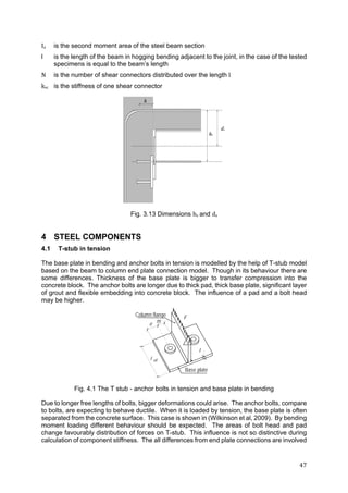
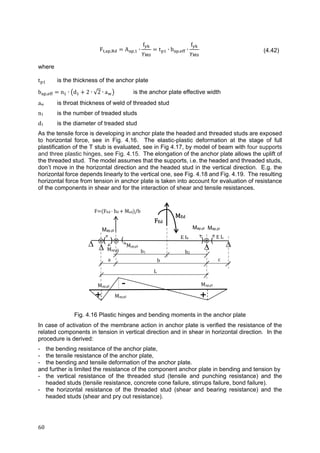
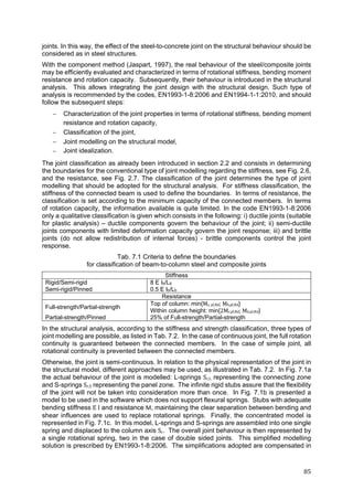
4.4 Anchor plate in bending and tension
The anchor plate is designed as a thin steel plate located at the top of concrete block and
loaded predominantly in compression and shear. By loading the column base by the bending
or tension is the anchor plate exposed to the tensile force from the treaded studs. If the
threaded studs are not located directly under the headed studs, which are embedded in
concrete, the anchor plate is exposed to bending, see Fig. 2.15. After the plastic hinges of the
T-stub are developed, the anchor plate between the plastic hinges is elongates by tensile force.
Base plate and anchor plate T stub plastic deformation under threaded stud
Plastic hinges at anchor plate Anchor plate elongation under the threaded stud
Fig. 4.15 Model of the anchor plate in bending and tension
The resistance of the component, see (Kuhlman et al, 2012), is not restricted to plastic
mechanism only. The deformed shape with the elongated anchored plate between the
threaded and headed studs is caring the additional load and may be taken into account. The
behaviour, till the plastic hinges are developed, is modelled as the based plate in bending with
help of T stub model, see Chapter 3.4. The anchor plate in tension resistance is](https://image.slidesharecdn.com/boltdesign-manualiien-191004025827/85/Bolt-design-manual-ii-en-60-320.jpg)
![61
- the interaction in the threaded stud (tension and shear resistances) and the headed studs
(tension and shear resistances).
The plastic resistance of the anchor plate is
M ,
l , t
4
f
γ
(4.43)
where
tp1 is thickness of the anchor plate [mm]
leff,1 is the effective width of the anchor plate [mm]
The effective width of the anchor plate is minimum of the
l , min
4 m 1.25 e
2 π m
5 n d ∙ 0.5
2 m 0.625 e 0.5 p
2 m 0.625 e e
π m 2 e
π m p
(4.44)
where 5 h d is the effective width of the T stub between the headed and threaded studs.
The vertical deformation of the anchor plate under bending may be assumed for a beam with
four supports and three plastic hinges as
δ
1
E I
∙
1
6
∙ b ∙ M ,
1
E I
∙
1
3
∙ b ∙ c ∙ M ,
(4.45a)
The elastic part of the deformation is
δ ,
2
3
∙ δ
(4.45b)
The elastic-plastic part of the deformation, see Fig. 4.17, is
δ , 2.22 δ ,
(4.45c)
The force at the bending resistance of the anchor plate is evaluated from equilibrium of internal
forces
N ∙ δ ∙
b
b
M ∙
δ
b
2 ∙ M , ∙
δ
a
2 ∙ M , ∙
δ
b
(4.45)
N ∙ b M 2 ∙ M , ∙ b ∙
1
a
1
b
(4.46)
for M N ∙ e
is N ∙ b N ∙ e 2 ∙ M , ∙ b ∙
1
a
1
b
(4.47)](https://image.slidesharecdn.com/boltdesign-manualiien-191004025827/85/Bolt-design-manual-ii-en-62-320.jpg)


![95
Fig. 7.7b Identification of the equivalent cross-sections of the beams in sub-structure II
Fig. 7.7c Identification of the equivalent cross-sections of the beams in each sub-structure III
Joint properties
The boundaries values for classification of the joint in terms of rotational stiffness and
resistance are listed in Tab. 7.8 for the three sub-structures. The joints were included in the
structural models using concentrated flexural springs. For the partial-strength joints, a tri-linear
behaviour was assigned, Fig. 7.8. The initial joint rotational stiffness is considered up to 2/3
of Mj,Rd, and then the joint rotation at Mj,Rd is determined using the secant joint rotational
stiffness. The latter is determined using a stiffness modification coefficient η equal to 2.
Tab. 7.8 The boundary values for classification of the joints in each sub-structure
Joints
Rotational Stiffness Bending Moment Resistance
R-SR [kNm/rad] SR-P [kNm/rad] FS-PS [kNm] PS-P [kNm]
Sub-structureI
AL-1-right
AL-2-left
AL-2-right
AL-3-left
AL-3-right
AL-4-left
108780.0
108780.0
205340.0
205240.0
108780.0
108780.0
2782.5
2782.5
3710.0
3710.0
2782.5
2782.5
351.4
358.9
358.9
345.0
351.4
351.4
87.9
89.7
89.7
87.5
85.9
87.9
Sub-structureII
AL-A-right
AL-B-left
AL-B-right
AL-C-left
to
AL-D-right
AL-E-left
AL-E-right
AL-F-left
102293.3
102293.3
94640.0
94640.0
94640.0
102293.3
102293.3
2660.0
2660.0
2100.0
2100.0
2100.0
2660.0
2660.0
274.9
286.9
286.9
292.1
286.9
286.9
274.9
68.7
71.7
71.7
73.0
71.7
71.7
68.7
Sub-structureIII
AL-A-right
AL-B-left
AL-B-right
to
AL-F-left
AL-F-right
AL-G-left
238560.0
238560.0
238560.0
238560.0
238560.0
7056.0
7056.0
7591.5
7056.0
7056.0
988.9
As below
b-6th
: 1058.1
6th
-T:380.4
As above
988.9
247.2
As below
b-6th
: 264.3
6th
-T: 95.1
As above
247.2
R-Rigid; SR-Semi-rigid; P-Pinned; FS-Full-strength; PS-Partial-strength
EqCS-1
EqCS-2
EqCS-3
EqCS-3
EqCS-4
EqCS-5
EqCS-5
EqCS-4
EqCS-5
EqCS-5
EqCS-4
EqCS-3
EqCS-3
EqCS-2
EqCS-1
2,25m
1,125m
1,125m
2,25m
2,25m
4,5m
2,25m
2,25m
4,5m
2,25m
2,25m
4,5m
2,25m
1,125m
1,125m
A B C D E FEqCS-1
EqCS-2
EqCS-3
EqCS-3
EqCS-2
EqCS-3
EqCS-3
EqCS-2
EqCS-3
EqCS-3
EqCS-2
EqCS-3
EqCS-3
EqCS-2
EqCS-3
EqCS-3
EqCS-2
EqCS-1
2,5m
2,5m
2,5m
2,5mv
2,5m
2,5m
2,5m
2,5m
2,5m
2,5m
2,5m
2,5m
5m
5m
5m
5m
5m
5m
BA C D E F G](https://image.slidesharecdn.com/boltdesign-manualiien-191004025827/85/Bolt-design-manual-ii-en-96-320.jpg)

![98
Fig. 7.9 Representation of the considered beams deflection
Tab. 7.11 Maximum beams deformation under service limit state [mm]
Case
Sub-structure I Sub-structure II Sub-structure III
Joint PropertiesBeam
1-2
Beam
3-4
Beam
C-D
Beam
A-B
Beam
C-D
Beam
F-G
1 2.6 3.0 5.5 0.3 21.7 7.7 R FS
2 3.3 3.2 7.8 0.3 22.9 12.7
↓ ↓
3 3.3 3.5 7.8 0.4 23.4 12.6
4 3.3 3.6 7.8 0.4 23.7 12.6
5 3.3 3.5 7.8 0.4 23.7 14.1
6 3.3 3.6 7.8 0.4 24.1 14.1
7 3.3 3.5 7.8 0.4 24.7 18.8
8 3.3 3.6 7.8 0.4 25.2 18.8
9 3.2 4.6 7.8 0.6 28.1 15.1
10 6.1 6.1 20.5 1.5 31.8 27.1 P P
δmax [mm] 20 20 30 15 33.3 33.3
R-Rigid; P-Pinned; FS-Full-strength
a) Sub-structure I b) Sub-structure II
c) Sub-structure III
Fig. 7.10 Beam deformations envelop and limit according to PNA to EN1993-1-1:2006
supported by a steel-to-concrete joint
δ](https://image.slidesharecdn.com/boltdesign-manualiien-191004025827/85/Bolt-design-manual-ii-en-99-320.jpg)
![99
Besides the beams deformation, the lateral stiffness of the sub-structures is also affected by
the joint properties. In Tab. 7.12 are listed the maximum top floor displacements obtained for
each case and for Sub-structures I and II. The design limit dh,top,limit according to Portuguese
National Annex to EN1993-1-1:2006 is also included. As for the beams deflections, it is
observed that the observed values are distant from the code limit. Note that as long as the
joints are continuous or semi-continuous, the top floor displacement suffers small variations.
This is due to the dominant contribution of the RC wall to the lateral stiffness of the sub-
structures. In Fig. 7.11 are represented the sub-structures lateral displacement envelops and
the code limit. In Sub-structure II, because two RC walls contribute to the lateral stiffness of
the sub-structure, the variation between minimum and maximum is quite reduced.
Tab. 7.12 Top floor lateral displacement for Sub-structures I and II [mm]
Case Sub-structure I Sub-structure II Joint Properties
1 26.7 13.5 R FS
2 27,6 14.0
↓ ↓
3 28.3 14.1
4 28.6 14.2
5 28.3 14.1
6 28.6 14.2
7 28.3 14.1
8 28.6 14.2
9 31.4 14.8
10 36.0 16.2
dh.top.limit [mm] 94.3 94.3 P P
R-Rigid; P-Pinned; FS-Full-strength
Sub-structure I Sub-structure II
Fig. 7.11 Lateral displacements envelops
In what concerns the steel-to-concrete joints, under service limit state, the bending moment
developed in the joints and the required joint rotation are represented in Fig. 7.12. In Fig. 7.13
the ratio between the bending moment developed in the joints and the joint or beam bending
moment capacity is represented. For none of the cases, the joints under SLS attained the
maximum bending moment resistance of the joint. As for the deformations, Sub-structure III
is the most demanding to the joints. In case 7, almost 70% of the joint bending moment
capacity is activated. Because the assumed joint resistance is lower, in case 7 and 8 the
percentage of bending moment activated is higher. In Fig. 7.13 is shown the maximum joint
rotations observed for each sub-structure and for each case. For the cases where the joints
are modelled as pinned, the joint rotation required is naturally higher, but never greater than
11 mrad. In the other cases, the joint rotation is quite low, below 3.2 mrad, which is expectable
as not plastic deformation of the joints occurs.
0
1
2
3
4
5
6
7
8
0 20 40 60 80 100
Floor
Lateral displacement [mm]
Case 1
Case 10
Limit
0
1
2
3
4
5
6
7
8
0 20 40 60 80 100
Floor
Lateral displacement [mm]
Case 1
Case 10
Limit](https://image.slidesharecdn.com/boltdesign-manualiien-191004025827/85/Bolt-design-manual-ii-en-100-320.jpg)
![100
Fig. 7.12 Ratio between acting bending moment and bending moment capacity
of joint/beam under SLS
Fig. 7.13 Joint rotation under SLS
7.2.5 Analysis and discussion for Ultimate Limit State
At Ultimate Limit State (ULS), joints should perform so that the structural integrity is not lost.
This requires to the joints either resistance either deformation capacity, allowing the
redistribution of internal forces within the structure. In order to quantify such structural demands
to the steel-to-concrete joints, calculations considering the load combinations of this limit state
are performed. In Fig. 7.14 are summarized the maximum loads obtained on these joints Mj,
Nj, Vj. In all cases, hogging bending moment and the axial compression are reported. Though,
it should be referred that axial tension is observed in bottom floors of the sub-structures;
however, in average, the maximum value does not exceed 10 kN.
0
0.1
0.2
0.3
0.4
0.5
0.6
1 2 3 4 5 6 7 8
Mj,Ed/[Mj,RdorMb,pl,Rd[-]
Case
Sub-structure I
Sub-structure II
Sub-structure III
0
2
4
6
8
10
12
1 2 3 4 5 6 7 8 9 10
Φj[mrad]
Case
Sub-structure I
Sub-structure II
Sub-structure III](https://image.slidesharecdn.com/boltdesign-manualiien-191004025827/85/Bolt-design-manual-ii-en-101-320.jpg)
![101
Tab. 7.13 Top floor lateral displacement for Sub-structures I and II
Sub-structure I Sub-structure II Sub-structure III
Joint
Properties
Joint
Location
AL-
3-L
AL-3-
R
AL-
3-L
AL-
F-L
AL-
A-R
AL-F-
L
AL-G-L
AL-
A-R
AL-
A-L
Case
Mj
[kNm]
Nj
[kN]
Vj
[kN]
Mj
[kNm]
Nj
[kN]
Vj
[kN]
Mj
[kNm]
Nj
[kN]
Vj
[kN]
1 169.0 68.5 181.1 64.7 31.8 72.9 441.1 387.6 345.8 R FS
2 170.0 61.7 183.3 65. 33.4 73.9 539.5 406.4 371.4
↓ ↓
3 151.2 62.3 178.3 54.2 31.5 70.8 406.4 392.6 362.3
4 136.2 62.8 174.3 46.2 30.1 68.7 350.4 382.1 355.6
5 151.2 62.3 178.3 54.2 31.5 70.8 432.1 384.0 381.6
6 136.3 62.8 174.3 46.2 30.1 68.7 376.1 372.5 376.1
7 138.0 62.1 174.8 54.8 33.0 71.3 401.9 381.3 394.5
8 121.7 62.4 170.5 46.6 31.6 69.2 344.7 371.9 388.9
9 0 65.9 138.9 0 21.0 56.5 0 282.4 346.5
10 0 43.3 134.0 0 51.7 59.4 0 346.7 370.9 P P
AL-Alignment; L – Left hand side; R- right hand side; R – Rigid; P – Pinned; FS – Full Strength
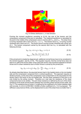
Fig. 7.14 shows the ratio between acting bending moment and the bending moment capacity
of the steel-to-concrete joints or of the beams, in the case of full strength joints. As expected,
for this limit state the ratio increases in comparison to the service limit state though, in none of
the cases the full capacity of joints is activated. The higher ratios are observed in Sub-
structures I and III, for the cases with lower bending moment resistance.
In Fig. 7.15 are plotted the maximum joint rotations observed in the different calculations. The
maximum required joint rotation is approximately 20 mrad for the case studies where the steel-
to-concrete joints are modelled as simple joints.
Fig. 7.14 Ratio between acting bending
moment and bending moment capacity of
joints, and beam at ULS
Fig. 7.15 Maximum joint rotation at ULS
0
0.2
0.4
0.6
0.8
1
1.2
1 2 3 4 5 6 7 8
Mj,Ed/[Mj,RdorMb,pl,Rd[-]
Case
Sub-structure I
Sub-structure II
Sub-structure III
0
5
10
15
20
25
1 2 3 4 5 6 7 8 9 10
Φj[mrad]
Case
Sub-structure I
Sub-structure II
Sub-structure III](https://image.slidesharecdn.com/boltdesign-manualiien-191004025827/85/Bolt-design-manual-ii-en-102-320.jpg)


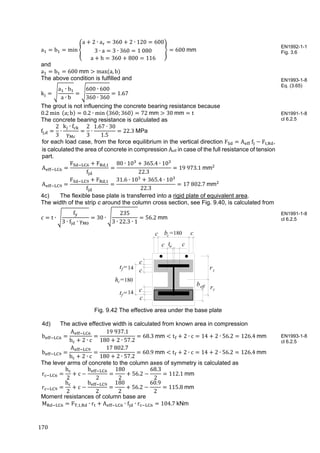
![118
N , 2 ∙ 300 ∙
π
4
∙
40 22
1.5
350.6 kN
δ , , 2 ∙ 0.0130 ∙
149 565
π
4
∙ 40 22 ∙ 25 ∙ 2
0.096 0.21 mm
The stiffness as a function of displacement is obtained using equations (3.34) and
(3.35) as:
k ,
π
4
∙ 40 22 ∙ 25 ∙ 2
0.0130 ∙ δ
384 373
δ
k ,
π
4
∙ 40 22 ∙ 25 ∙ 2
2 ∙ 0.0130 ∙ δ
δ 0.096
271 792
δ
∙ δ 0.096
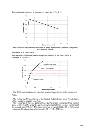
The load-displacement curve for the spring is shown in Fig. 9.12.
Fig. 9.12 Load-displacement behaviour of spring representing component P
3.6 Interaction of components Concrete and Stirrups
Once the concrete breakout occurs, the load is transferred to the stirrups and the load
shared by concrete decreases with increasing displacement. The load carried by the
combined component concrete + stirrups corresponding to any given displacement is
given by Eq. (3.59) as
N N , k , δ min n d ,
α f δ
2
; N , , ; N , ,
Hence, for a given displacement δ [mm] the load [kN] carried by combined concrete and
stirrups is given as
N 119.0 50.31 ∙ δ min 448.023√δ; 393.6; 149.6
DM I
Eq. (3.34)
DM I
Eq. (3.35)
DM I
Eq. (3.59)
DM I
Eq. (3.59)
0
50
100
150
200
250
300
350
400
0 0.25 0.5 0.75 1 1.25 1.5 1.7
Axialload,N(kN)
Displacement, δ (mm)](https://image.slidesharecdn.com/boltdesign-manualiien-191004025827/85/Bolt-design-manual-ii-en-119-320.jpg)


![131
ψ 2.5
x
h
2.5
d
2
d ,
d ,
tan 35°
h
2.5
d
2
5 ∙
d
2
d
2
d
2
10
tan 35°
h
2.5
22
2
5 ∙
8
2
22
2
8
2
10
tan 35°
200
2.3
and resistance
N ,
ψ ∙ N ,
γ
2.3 ∙ 230.2
1.5
353.0 kN
with
k , α ∙ f ∙ h ∙ ψ , ∙ ψ , ∙ ψ , 537 ∙ √30 ∙ 200 ∙ 1.17 ∙ 1.0 ∙ 1.0
48.7 kN/mm
where
αc = -537 is factor of component concrete break out in tension
Yielding of reinforcement will occur for
N , N , , N , δ , ∙ k ,
A , ∙
f ,
γ
N ,
2 ∙ N , ,
α ∙ f ∙ d , ∙ n ∙ n
∙ k ,
n ∙ n ∙ π ∙ ,
∙
,
N ,
∙ ∙ ∙ ∙ ,
∙
,
∙ ∙ , ∙ ∙
∙ k , =
2 ∙ 4 ∙ π ∙
8
4
∙
500
1.15
153.5
2 ∙ 2 ∙ 4 ∙ π ∙
8
4
∙
500
1.15
12100 ∙ 30 ∙ 8 ∙ 2 ∙ 4
∙ 48.7
174.8 153.5 0.642 ∙ 48.7 297.0 kN
where
αs = 12 100 is factor of the component stirrups
nre = 4 is total number of legs of shafts
NRd,s,re is design tension resistance of the stirrups for tension failure [N]
ds,re = 8 mm is nominal diameter of the stirrup
dp = 25 mm is the covering
fyk,s = 500 N/mm2 is design yield strength of the stirrups
γMs = 1.15 is the partial safety factor
l1 is anchorage length [mm]
Anchorage failure resistance of the of reinforcement is
DM I
Eq. (3.48)
DM I
Eq. (3.47)
DM I
Eq. (3.13)
DM I
Eq. (3.16)
DM I
Eq. (3.16)](https://image.slidesharecdn.com/boltdesign-manualiien-191004025827/85/Bolt-design-manual-ii-en-132-320.jpg)
![132
N , N , , N , δ , ∙ k , n ∙ l π ∙ d , ∙
f
α
N , δ , ∙ k ,
n ∙ n ∙ l ∙ π ∙ d ∙
f
α
N ,
2 ∙ N , ,
α ∙ f ∙ d , ∙ n
∙ k ,
n ∙ n ∙ h d d ,
d ,
1.5
∙ π ∙ d ∙
2.25 ∙ η ∙ η ∙ f ; ,
α ∙ γ
N ,
2 ∙ n ∙ n ∙ l ∙ π ∙ d ∙
f
α
α ∙ f ∙ d , ∙ n
k ,
n ∙ n ∙ h d 10
∙
.
∙ π ∙ d ∙
. ∙ ∙ ∙ ; ,
∙
N ,
∙ ∙ ∙
∙
.
∙ ∙ ∙
. ∙ ∙ ∙ ; ,
∙
∙ ∙ , ∙
∙ k , =
2 ∙ 4 ∙ 200 25
8
2
10
5 ∙
8
2
22
2
1.5
∙ π ∙ 8 ∙
2.25 ∙ 1.0 ∙ 1.0 ∙ 2.0
0.49 ∙ 1.5
153.5
2 ∙ 2 ∙ 4 ∙ 200 25
8
2
10
5 ∙
8
2
22
2
1.5
∙ π ∙ 8 ∙
2.25 ∙ 1.0 ∙ 1.0 ∙ 2.0
0.49 ∙ 1.5
12100 ∙ 30 ∙ 8 ∙ 2 ∙ 4
∙ 48.7
190.8 153.5 0.765 ∙ 48.7 307.0 kN
where
l1 is anchorage length [mm]
ds is diameter of stirrups [mm]
α 0.7·0.7 = 0.49 is factor for hook effect and large concrete cover
fbd is for C30/37 grade concrete is 2.25 ∙
.
.
1.0 1.0 3.0 N/mm2
η1 1.0 is coefficient of bond conditions for vertical stirrups
and 0.7 for horizontal stirrups
η2 = 1.0 is coefficient of bond conditions for dimension ≤ 32 mm
and (132 - ds)/100 for dimension ≥ 32 mm
The resistance of concrete cone failure with reinforcement is
min N , ; N , ; N , min 353.0; 297.0; 307.0 297.0 kN
DM I
Eq. (3.20)
DM I
Eq. (3.21)
EN1992-1-1](https://image.slidesharecdn.com/boltdesign-manualiien-191004025827/85/Bolt-design-manual-ii-en-133-320.jpg)


![155
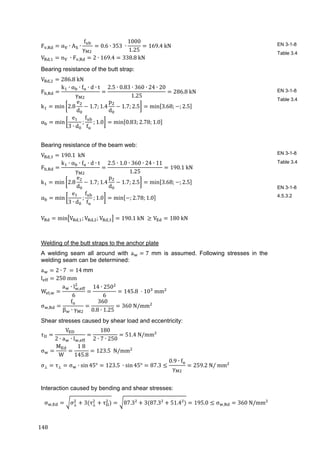
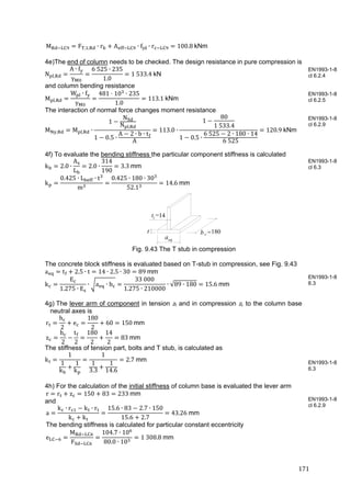
9.6 Moment resistant steel to concrete joint
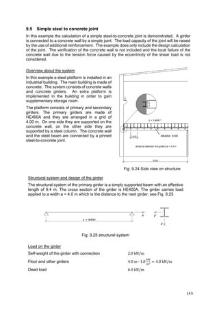
The steel-to-concrete connection is illustrated in Fig. 9.27. It represents the moment-resistant
support of a steel-concrete-composite beam system consisting of a hot rolled or welded steel
profile and a concrete slab, which can either be added in situ or by casting semi-finished
precast elements. Beam and slab are connected by studs and are designed to act together.
Whereas the advantage of the combined section is mostly seen for positive moments, where
compression is concentrated in the slab and tension in the steel beam, it may be useful to use
the hogging moment capacity of the negative moment range either as a continuous beam, or
as a moment resistant connection. In this case, the reinforcement of the slab is used to raise
the inner lever arm of the joint. The composite beam is made of a steel profile IPE 300 and a
reinforced concrete slab with a thickness of 160 mm and a width of 700 mm. The concrete
wall has a thickness of 300 mm and a width of 1 450 mm. The system is subjected to a hogging
bending moment ME,d = 150 kNm. Tabs 9.1 and 9.2 summarize data for the steel-to-concrete
joint.
Fig. 9.27: Geometry of the moment resisting joint
Tab. 9.1 Geometry for the steel-to-concrete joint
Geometry
RC wall RC Slab Anchors
t [mm] 300 t [mm] 160 d [mm] 22
b [mm] 1450 b [mm] 700 dh [mm] 35
h [mm] 1600 l [mm] 1550 la [mm] 200
Reinforcement Reinforcement hef [mm] 215
Φv [mm] 12 Φl [mm] 16 nv 2
nv 15 nl 6 e1 [mm] 50
sv [mm] 150 sl [mm] 120 p1 [mm] 200
Φh [mm] 12 Φt [mm] 10 nh 2
nh 21 nt 14 e2 [mm] 50
sh [mm] 150 st [mm] 100 p2 [mm] 200
ctens,bars [mm] 30
rhook [mm] 160
Console 1 Console 2 Anchor plate
t [mm] 20
200
150
t [mm] 10
170
140
tap [mm] 15
b [mm] b [mm] bap [mm] 300
h [mm] h [mm] lap [mm] 300
Shear Studs Steel beam IPE 300 Contact Plate
d [mm] 22
100
9
140
270
90
h [mm] 300 t [mm] 10
hcs [mm] b [mm] 150 bcp [mm] 200
Nf tf [mm] 10.7 lcp [mm] 30
s [mm] tw [mm] 7.1 e1,cp [mm] 35
a [mm] As [mm2
] 5381 eb,cp [mm] 235
hc [mm] bap [mm] 300](https://image.slidesharecdn.com/boltdesign-manualiien-191004025827/85/Bolt-design-manual-ii-en-156-320.jpg)
![156
The part of the semi-continuous joint configuration, within the reinforced concrete wall,
adjacent to the connection, is analyzed in this example. This has been denominated as “Joint
Link”. The main objective is to introduce the behaviour of this component in the global analysis
of the joint which is commonly disregarded.
Tab. 9.2 Material of the steel-to-concrete joint
Concrete wall Concrete slab Rebars wall
fck,cube [Mpa] 50 fck,cube [Mpa] 37 fsyk [MPa] 500
fck,cyl [Mpa] 40 fck,cyl [Mpa] 30 fu [Mpa] 650
E [GPa] 36 E [GPa] 33
fctm [Mpa] 3.51 fctm [Mpa] 2.87
Rebars Slab Steel Plates Anchors
fsyk [Mpa] 400 fsyk [Mpa] 440 fsyk [Mpa] 440
fu [Mpa] 540 fu [Mpa] 550 fu [Mpa] 550
εsry [‰] 2 Steel Profile Shear Studs
εsru 75 fsyk [Mpa] 355 fsyk [Mpa] 440
fu [Mpa] 540 fu [Mpa] 550
The design value of the modulus of elasticity of steel Es may be assumed to be 200 GPa.
Fig. 9.28 Activated joint components
In order to evaluate the joint behaviour, the following basic components are identified, as
shown in Fig. 9.28:
- longitudinal steel reinforcement in the slab, component 1
- slip of the composite beam, component 2;
- beam web and flange, component 3;
- steel contact plate, component 4;
- components activated in the anchor plate connection, components 5 to 10 and 13 to 15;
- the joint link, component 11.
Step 1 Component longitudinal reinforcement in tension
In this semi-continuous joint configuration, the longitudinal steel reinforcement bar is the only
component that is able to transfer tension forces from the beam to the wall. In addition, the
experimental investigations carried (Kuhlmann et al., 2012) revealed the importance of this
component on the joint response. For this reason, the accuracy of the model to predict the
joint response will much depend on the level of accuracy introduced in the modelling of this
component. According to ECCS Publication Nº 109 (1999), the behaviour of the longitudinal
steel reinforcement in tension is illustrated in Fig. 9.29.](https://image.slidesharecdn.com/boltdesign-manualiien-191004025827/85/Bolt-design-manual-ii-en-157-320.jpg)
![159
is the length of the reinforcement up to the beginning of the bend. sm is the average bond
stress, given by
τ 1.8 ∙ f
Forces can be evaluated considering minimum values of tensions found for slab and wall.
Table 9.3 summarizes the results for the stress-strain and force-displacement curves.
Tab. 9.3 Force-displacement relation for longitudinal reinforcement in tension
σSL
[N/mm2
]
SL
[-]
σWA
[N/mm2
]
WA
[-]
F
[kN]
Δr
[mm]
97.1 3.0 · 10-5
118.7 3.6 · 10-5
117.1 0.0
126.2 4.9· 10-4
154.3 5.9· 10-4
152.3 0.1
347.8 1.6 · 10-3
347.8 1.6 · 10-3
419.6 0.3
469.5 4.4 · 10-2
469.5 4.0 · 10-2
566.5 5.7
Step 2 Component slip of composite beam
The slip of composite beam is not directly related to the resistance of the joint; however,
the level of interaction between the concrete slab and the steel beam defines the maximum
load acting on the longitudinal reinforcement bar. In EN 1994-1-1: 2010, the slip of
composite beam component is not evaluated in terms of resistance of the joint, but the
level of interaction is considered on the resistance of the composite beam. However, the
influence of the slip of the composite beam is taken into account on the evaluation of the
stiffness and rotation capacity of the joint. The stiffness coefficient of the longitudinal
reinforcement should be affected by a reduction factor kslip determined according to Chap.
3.7.
According to (Aribert, 1995) the slip resistance may be obtained from the level of interaction
as expressed in the following. Note that the shear connectors were assumed to be ductile
allowing redistribution of the slab-beam interaction load.
F N ∙ P
Where: N is the real number of shear connectors; and PRK is characteristic resistance of the
shear connectors that can be determined according to EN1994-1-1:2010 as follows
P min
0.8 ∙ f ∙ π ∙ d
γ ∙ 4
;
0.29 ∙ α ∙ d f ∙ E
γ
with
3 4 α 0.2 1
4 α 1
where fu is the ultimate strength of the steel shear stud; d is the diameter of the shear stud;
fck is the characteristic concrete cylinder resistance; Ecm is the secant modulus of elasticity
of the concrete; hsc is the height of the shear connector including the head; γ is the partial
factor for design shear resistance of a headed stud.
P min
0.8 ∙ 540 ∙ π ∙ 22
1.25 ∙ 4
;
0.29 ∙ 1 ∙ 22 ∙ 30 ∙ 33
1.25
min 486.5; 111.0 111.0 kN
F 9 ∙ 111.0 999.0 kN
Concerning the deformation of the component, assuming an uniform shear load distribution
along the beam, an equal distribution of the load amongst the shear studs is expected.
EN1994-1-
1:2010](https://image.slidesharecdn.com/boltdesign-manualiien-191004025827/85/Bolt-design-manual-ii-en-160-320.jpg)

![163
Δ 6.48 10 F , 7.47 10 F , ∙ cos θ
Thus, considering 10 load steps, Tab. 9.4 summarizes the force-displacement curve.
Tab. 9.4 Force-displacement for the Joint Link component
Fh [kN] Δh [mm]
0.0 0.00
61.1 0.00
122.1 0.00
183.2 0.01
244.2 0.01
305.3 0.01
366.3 0.02
427.4 0.02
488.5 0.03
549.5 0.03
610.6 0.03
Step 7 Assembly of joint
The simplified mechanical model represented in Fig. 9.32 consists of two rows, one row
for the tensile components and another for the compression components. It combines the
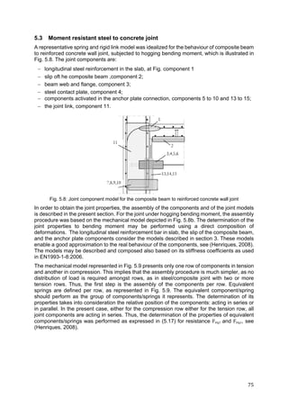
tension and compression components into a single equivalent spring per row.
Fig. 9.32: Simplified joint model with assembly of components per row
The properties of the equivalent components/springs are calculated, for resistance, Feq,t
and Feq,c, and deformation, Δeq,t and Δeq,c, as follows
F min F to F
∆ ∆
where index i to n represents all relevant components, either in tension or in compression,
depending on the row under consideration.
According to the joint configuration, it is assumed that the lever arm is the distance between
the centroid of the longitudinal steel reinforcement bar and the middle plane of the bottom
flange of the steel beam. The centroid of the steel contact plate is assumed aligned with
this reference point of the steel beam. Hence, the bending moment and the corresponding
rotation follow from
M min F , ; F , ; F ∙ h Φ
Δ , Δ , Δ
h
Thus
Ft,max = 566.5 kN Longitudinal rebar
Fc,max = 610.6 kN Joint link](https://image.slidesharecdn.com/boltdesign-manualiien-191004025827/85/Bolt-design-manual-ii-en-164-320.jpg)
![164
Feq = 566.5 kN
hr = 406.65 mm
Mj = 230.36 KNm
Table 9.5 summarizes the main results in order to calculate the moment rotation curve,
where Δr is the displacement of the longitudinal steel reinforcement, Δslip is related to the
slip of composite beam through to the coefficient kslip, ΔT-stub is the displacement of the T-
stub in compression and ΔJL is the displacement of the joint link.
Tab. 9.5 Synthesis of results
F
[kN]
Δr
[mm]
Δslip
[mm]
ΔT‐stub
[mm]
ΔJL
[mm]
Δt
[mm]
Φ
[mrad]
Mj
[kNm]
0.0 0.00 0.00 0.00 0.00 0.00 0.00 0.00
117.1 0.01 0.13 0.03 0.00 0.17 0.40 47.64
152.3 0.09 0.17 0.04 0.01 0.30 0.73 61.93
419.6 0.27 0.47 0.12 0.02 0.88 2.06 170.63
566.5 5.68 0.63 0.16 0.03 6.36 15.53 230.36
Note
The resulting moment-rotation behaviour is shown in Fig. 9.33. The system is able to resist
the applied load.
Fig. 9.33 Joint bending moment-rotation curve Mj ‐ Фj](https://image.slidesharecdn.com/boltdesign-manualiien-191004025827/85/Bolt-design-manual-ii-en-165-320.jpg)
![167
Fig. 9.35 System with max bending
moment from all combinations [kNm]
Fig. 9.36 System with min bending
moment from all combinations [kNm]
Fig. 9.37 System with min axial force
from all combinations [kN]
Fig. 9.38 Deformation
for wind in x-direction [mm]
Maximal deformation under variable load is 17 mm at the top.
Step 2 Verification of elements
Verifications are performed using the EC3 Steel Member Calculator for iPhone.
Column HEB 180 is verified as
Acting forces
from LC 6
Critical section
resistance
Buckling
resistance
Verification
Nmin,d = -80 kN Nc,Rd = -1533 kN Nb,y,Rd = -1394 kN
ε N My V ≤ 1
0.477
MAy,d = 51 kNm MyAy,c,Rd = 113.1 kNm Nb,z,Rd = 581 kN ε Mb Nby (6.61)) ≤ 1
0.265MB’y,d = 45 kNm Vc,Rd = 274 kN Mb,Rd = 102.8 kNm
Beam IPE 270 is verified as
Acting force
from LC 4
Critical cection
resistance
Buckling
resistance
Verification
Nmin,d = -19 kN Nc,Rd = 1079.7 kN
Mb,Rd = 103,4 kNm
ε N My V ≤ 1
0.536
MEy,d = 61 kNm My,c,Rd = 113.7 kNm ε Mb Nby (6,61)) ≤ 1
0.265MB’’y,d = -51 kNm Vc,Rd = 300.4 kN](https://image.slidesharecdn.com/boltdesign-manualiien-191004025827/85/Bolt-design-manual-ii-en-168-320.jpg)
![168
Step 3 Design of beam to column joint
The connection is illustrated in Fig. Fig. 9.39. The end plate has a height of 310 mm, a
thickness of 30 mm and a width of 150 mm with 4 bolts M20 10.9.
Design Values
My,Rd = -70.7 kNm > -54.5 kNm (at x = 0.09 of supports axis)
Vz,Rd = 194 kN
Fig. 9.39 Design of beam-to-column joint
The verification is performed using the ACOP software. The resulting bending moment –
rotation curve is represented in Fig. 9.40.
Fig. 9.40 The bending moment to rotation curve Mj ‐ Фj
Step 4 Verification of the column base joint
Main Data
- Base plate of 360 x 360 x 30 mm, S235
- Concrete block of size 600 x 600 x 800 mm, C30/37
- Welds aw,Fl = 7 mm, aw,St = 5 mm
- The support with base plate is in a 200 mm deep of the foundation.
Design Values
Characteristic LC Nx,d [kN] My,d [kNm]
Nmin 6 -80 51
Mmax 9 -31.6 95.6](https://image.slidesharecdn.com/boltdesign-manualiien-191004025827/85/Bolt-design-manual-ii-en-169-320.jpg)
![172
e
M
F
100.8 ∙ 10
31.6 ∙ 10
3 189.9 mm
as
S ,
e
e a
∙
E ∙ r
μ ∑
1
k
1 308.8
1 308.8 3 189.9
∙
210 000 ∙ 233
1 ∙
1
2.7
1
15.6
25 301 kNm/rad
S ,
e
e a
∙
E ∙ r
μ ∑
1
k
3 189.9
3 189.9 3 189.9
∙
210 000 ∙ 233
1 ∙
1
2.7
1
15.6
25 846 kNm/rad
These values of stiffness do not satisfy the condition about the rigid base
S , 30 E ∙ I /L 45 538 kNm/rad
Step 5 Updating of internal forces and moments
Steps 1 to 4 should be evaluated again considering internal forces obtained from a
structural analysis taking into account the stiffness of column base, see Fig. 9.44. Tab. 9.4
summarizes results of the structural analysis of the two meaning full combinations Nmin and
Mmax.
Fig. 9.44 Structural system with rotational springs
Tab. 9.4 Comparison of internal forces between the model with rigid column base joint and
the model with the actual stiffness
Load
case
Column base
stiffness
Point A Point B Point C Point D
N
[kN]
M
[kNm]
N
[kN]
M
[kNm]
N
[kN]
M
[kNm]
N
[kN]
M
[kNm]
6
Rigid -57.0 1.6 -54.0 27.7 -56.0 49.3 -80.0 51.0
Semi-rigid -56.9 3.1 -53.3 24.3 -57.1 -40.7 -80.8 48.4
9
Rigid -31.6 95.6 -29 -18.7 -29.0 -36.0 -47.0 32.6
Semi-rigid -30.5 87.3 -27.9 -17.7 -30.9 -40.6 -48.4 34.7
For the LC6 has been implemented a structural model with two rotational springs equal to
25 301 kNm/rad. For the LC9 the adopted rotational stiffness was equal to 25 846 kNm/rad.
Due to the proximity of the stiffness value calculated in Step 4. it was reasonable to
assumed in a simplified manner. The lower value of the stiffness in order to update the
internal forces of the system.
As shown in the above table, the differences in terms of internal forces are negligible and
therefore the single elements and the beam to column joint is considered verified. Tab. 9.4
synthetizes the updated properties of the column base joint.
EN1993-1-8
cl 6.3
EN1993-1-8
cl 5.2
A
B C
D](https://image.slidesharecdn.com/boltdesign-manualiien-191004025827/85/Bolt-design-manual-ii-en-173-320.jpg)
![173
Tab. 9.4 Updated properties of the column base joint
Load
case
Column base
stiffness
Aeff
[mm2
]
beff
[mm]
rc
[mm]
Mrd
[kNm]
S .
[kNm/rad
6
Rigid 19 973.1 68.3 112.1 104.7 25 301
Semi-rigid 20 008.0 68.4 112.0 104.8 25 268
9
Rigid 17 802.7 60.9 115.8 100.8 25 846
Semi-rigid 17 757.0 60.7 115.8 100.7 25 344
The designed column base fulfils the asked requirements as shown in the Tab. 9.4.](https://image.slidesharecdn.com/boltdesign-manualiien-191004025827/85/Bolt-design-manual-ii-en-174-320.jpg)


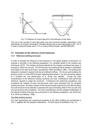
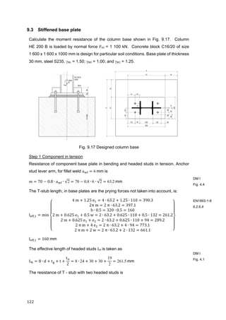
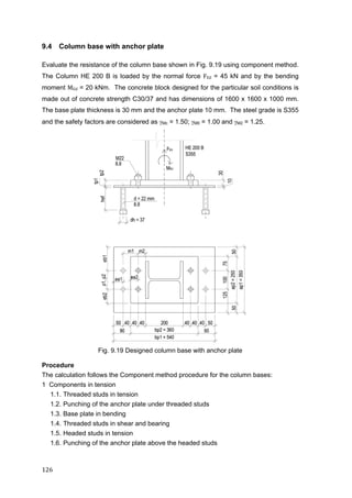
![Chyba! Pomocí karty Domů použijte u textu, který se
má zde zobrazit, styl Überschrift 1. Chyba! Pomocí karty Domů použijte u textu, který se má zde zobrazit, styl
Überschrift 1.
9
1 Introduction
1.1 Introduction and structure of the document
The mixed building technology allows to utilise the best performance of all structural materials available
such as steel, concrete, timber and glass. Therefore the building are nowadays seldom designed from only
one structural material. Engineers of steel structures in practice are often faced with the question of eco‐
nomical design of steel‐to‐concrete joints, because some structural elements, such as foundations, stair
cases and fire protection walls, are optimal of concrete. A gap in knowledge between the design of fastenings
in concrete and steel design was abridged by standardized joint solutions developed in the INFASO project,
which profit from the advantage of steel as a very flexible and applicable material and allow an intelligent
connection between steel and concrete building elements. The requirements for such joint solutions are
easy fabrication, quick erection, applicability in existing structures, high loading capacity and sufficient de‐
formation capacity. One joint solution is the use of anchor plates with welded headed studs or other fasten‐
ers such as post‐installed anchors. Thereby a steel beam can be connected by butt straps, cams or a beam
end plate connected by threaded bolts on the steel plate encased in concrete. Examples of typical joint so‐
lutions for simple steel‐to‐concrete joints, column bases and composite joints are shown in Fig. 1.1.
a) b) c)
Fig. 1.1: Examples for steel‐to‐concrete joints: a) simple joint, b) composite joint, c) column bases
The Design Manual II "Application in practice" shows, how the results of the INFASO projects can be simply
applied with the help of the developed design programs. For this purpose the possibility of joint design with
new components will be pointed out by using practical examples and compared with the previous realiza‐
tions. A parametric study also indicates the effects of the change of individual components on the bearing
capacity of the entire group of components. A detailed technical description of the newly developed com‐
ponents, including the explanation of their theory, can be found in the Design Manual I "Design of steel‐to‐
concrete joints"[13].
Chapter 2 includes a description of the three design programs that have been developed for the connection
types shown in Fig. 1.1. Explanations for the application in practice, the handling of results and informations
on the program structure will be given as well as application limits and explanations of the selected static
system and the components. Practical examples, which have been calculated by using the newly developed
programs, are included in Chapter 3. These connections are compared in terms of handling, tolerances and
the behaviour under fire conditions to joints calculated by common design rules. The significant increase of
the bearing capacity of the "new" connections under tensile and / or bending stress result from the newly
developed components "pull‐out" and "concrete cone failure with additional reinforcement". Chapter 4 con‐
tains parameter studies in order to show the influence of the change of a single component on the entire
group of components, and hence to highlight their effectiveness.](https://image.slidesharecdn.com/boltdesign-manualiien-191004025827/85/Bolt-design-manual-ii-en-188-320.jpg)

![Chyba! Pomocí karty Domů použijte u textu, který se
má zde zobrazit, styl Überschrift 1. Chyba! Pomocí karty Domů použijte u textu, který se má zde zobrazit, styl
Überschrift 1.
11
2 Program description
2.1 Restrained connection of composite beams
General
In the following the Excel sheet “Restrained connection of composite beams” (Version 2.0 Draft) [21] is
presented. With this program the load bearing capacity (moment and shear) of a fully defined joint, com‐
posed of tensional reinforcement in slab and cast‐in steel plate with headed studs and additional reinforce‐
ment at the lower flange of the steel section can be determined. The shear and the compression component,
derived from given bending moment, are acting on a welded steel bracket with a contact plate in‐between,
as the loading position on the anchor plate is exactly given. The tensional component derived from given
bending moment is transferred by the slab reinforcement, which is bent downwards into the adjacent wall.
Attention should be paid to this issue as at this state of modelling the influence of reduced distances to edges
is not considered. The wall with the cast‐in steel plate is assumed to be infinite in elevation. In this program
only headed studs are considered. Post installed anchors or similar have to be taken in further considera‐
tion.
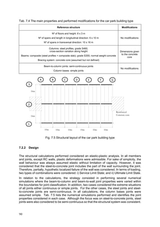
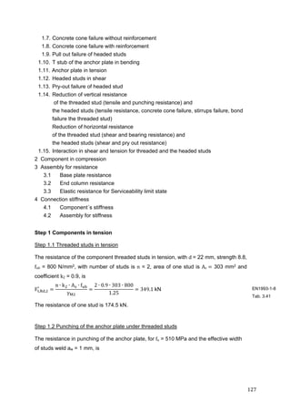
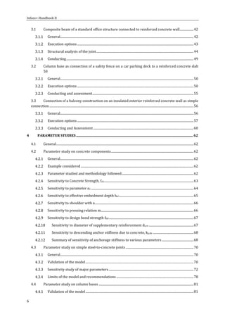
Program structure](https://image.slidesharecdn.com/boltdesign-manualiien-191004025827/85/Bolt-design-manual-ii-en-190-320.jpg)
![Infaso+‐Handbook II
12
The Excel file is composed of two visible
sheets. The top sheet contains full input, a
calculation button and the resulting load bearing capacity of the joint with utilization of bending moment
and shear (see Fig. 2.1). The second sheet gives the input data echo, with some additional calculated geom‐
etry parameters and the characteristic material properties. Subsequently it returns calculation values to
allow checking the calculation flow and intermediate data. Other sheets are not accessible to the user. One
contains data for cross sections (only hot rolled sections are considered), for headed studs and concrete.
The three other sheets are used to calculate tension in studs, shear resistance, anchor plate assessment and
stiffness values. Parameter and results are given in output echo (sheet 2). The user introduces data in cells
coloured in light yellow. All drawings presented are used to illustrate the considered dimensions and theory
used behind. They do neither change with input nor are drawn to scale. A check for plausibility will be exe‐
cuted for some input parameters, with warning but without abortion. The user has to interpret results on
own responsibility and risk. The majority of the calculations are performed introducing formulae in the
cells. However, when more complex calculation and iterative procedure is required, a macro is used to per‐
form these calculation. The user has to press the corresponding ‘Calculation’ button. If any changes in the
parameters are made the macro calculation should be repeated. By opening the worksheet the accessible
input cells (in yellow) are preset with reasonable default values. They must be changed by the user. Hot
rolled steel sections, steel and concrete grades, type and length of studs/reinforcement are implemented
with the help of a dropdown menu to choose one of the given parameters. To model the stiffness according
to the developed theory some additional information must be given in the top (input) sheet. The effective
width and length of slab in tension, the reinforcement actually built in and the number and type of studs
connection slab and steel beam. These information do not influence the load capacity calculations.
Input and output data and input data cells
The user inserts data only into cells coloured in light yellow. The accessible input cells are not empty but
preset per default with reasonable values. They can be changed by the user. The units given in the input
cells must not be entered, they appear automatically to remind the correct input unit.
Choice of appropriate code – whereas Eurocode EN 1992‐1‐1 [7] for design of reinforced concrete,
EN 1993‐1‐1 [8] for design of steel and EN 1994‐1‐1 [10] for steel‐concrete composite structures are the
obligatory base for all users, the national annexes must be additionally considered. For purpose of design
of connections to concrete it can be chosen between EN 1992‐1‐1 [7] in its original version and the appro‐
priate (and possibly altered) values according to national annex for Germany, Czech Republic, Portugal, the
UK, France and Finland. The input procedure should be self‐explaining, in context with the model sketch on
top of first visible sheet. According to this principal sketch of the moment resisting joint there are nine com‐
ponents and their input parameters necessary to define characteristics and geometry.
1. + 2. Composite beam of a hot rolled section of any steel grade acc. to EN 1993‐1‐1 [8] and a reinforced
concrete slab of any concrete grade acc. to EN 1992‐1‐1 [7]. They are connected by studs and working as a
composite structure according to EN 1994‐1‐1 [10]. This composite behaviour is only subject of this calcu‐
lation because it’s flexibility due to slip influences the connection stiffness. Following selections can be
made:
Type of sections: Hot rolled sections IPE, HEA, HEB, HEM of any height
Steel grades: S 235, S275, S355 acc. to EN 1993‐1‐1 [8] (EN‐10025)
Concrete grades: C20/25 until C50/60 acc. to EN 1992‐1‐1 [7]
Reinforcement grade: BSt 500 ductility class B acc. to EN 1992‐1‐1 [7]
3. Concrete wall – the shear and bending moment are to be transferred into the infinite concrete wall with
limited thickness. Per definition reinforcement and a cast‐in steel plate are used. It can be chosen between:
Concrete grades: C20/25 until C50/60 acc. to EN 1992‐1‐1 [7]
Reinforcement grade: Bst 500 ductility class B acc. to EN 1992‐1‐1 [7]
4. Anchor plate with studs – at the bottom flange of the steel section an anchor plate is inserted into the
concrete wall. Welded studs on the rear side transfer tensional (if any) and/or shear forces from top of
Fig. 2.1: EXCEL input file](https://image.slidesharecdn.com/boltdesign-manualiien-191004025827/85/Bolt-design-manual-ii-en-191-320.jpg)
![Chyba! Pomocí karty Domů použijte u textu, který se
má zde zobrazit, styl Überschrift 1. Chyba! Pomocí karty Domů použijte u textu, který se má zde zobrazit, styl
Überschrift 1.
13
anchor plate into the concrete. The compression components are transferred directly by contact between
the steel plate and the concrete.
Geometry of plate: Thickness and 2D‐dimensions and steel grade, single input values in
[mm], input check: thickness ≥ 8mm is deemed to be ok.
Type of studs: Köco resp. Nelson d19, d22, d25 regular or d19, d22 stainless steel, Peikko
d19, d20 regular or d20, d25 reinforcement bar with head all data
including steel grades from ETA‐approval (e.g. the steel grades are
considered automatically according to approval).
Length of studs: 75 until 525 mm (from ETA‐approval), input check: length less than wall
thickness less coverage and plate thickness is deemed to be ok.
Distribution studs: Number of studs (4,6,8) and inner distances, input check: distances to lay
within plate are deemed to be ok
5. Steel bracket is welded on top of the anchor plate and takes the shear force with small eccentricity and
transfers it into the anchor plate /concrete wall.
Geometry of plate: Thickness and 2D‐dimensions, ‘nose’ thickness, input check: width and
height less than anchor plate is deemed to be ok. Position/eccentricity is
required in 6. Contact plate.
6. Contact plate – the contact plate is inserted force‐fit between the end of the steel section and the anchor
plate at lower flange level. The compression force component from negative (closing) bending moment is
transferred on top of anchor plate.
Geometry of plate: Thickness and 2D‐dimensions, eccentricity of plate position in relation to
anchor plate centre. Input check: width less than anchor plate and position
within anchor plate is deemed to be ok.
7. Reinforcement bars – in the slab of the composite section. The tensional force component from negative
(closing) bending moment is transferred into the wall and bent down on the rear face of the wall and an‐
chored there. Whereas the necessary design reinforcement is calculated by the work sheet, for later use of
stiffness calculation, the existing reinforcement in the slab of the composite beam is required. The bar di‐
ameter should be chosen in a way that reasonable spacings within the effective width result and that the
bend can be installed within the wall. The length of tension zone is crucial for the stiffness evaluation and
depends on the structural system. It must be chosen in accordance with codes or independent calculation
results of the underlying model (Example: in case of beam simply supported and other side restrained it is
≈ 0,25 *length, in case of cantilever beam it is 1,0*length)
Bars: steel area [cm²], diameter and length of tension zone [cm], input check:
reinforcement must be ≥ minimum design reinf. area, spacing of bars should be
within interval 5‐25 cm, bar curvature Ø*20 must fit into wall.
8. Additional stirrups – these optional stirrups are proposed as an effective means to improve the joint in
case of tension forces (if any, only in case of small moments and large shear force with large eccentricity) in
the stud. They are useful only in the upper row, and only under certain circumstances of the complete as‐
semblage. Further information can be found in the parameter study in Chapter 4. Generally there is always
a surface reinforcement in the front face of the wall. This may be optionally taken into account and will
improve the capacity of the joint under certain circumstances of the complete assemblage.
Reinforcement: bar‐diameter of stirrups with legs each very close to studs (default: no
stirrup, input range Ø8‐14 mm), and surface reinforcement bar‐diameter
(Ø6‐14 mm) and spacing (75‐250 mm)](https://image.slidesharecdn.com/boltdesign-manualiien-191004025827/85/Bolt-design-manual-ii-en-192-320.jpg)
![Infaso+‐Handbook II
14
9. Slab studs – these studs are welded at the upper flange of the steel cross section and are the connection
medium in the joint between steel and concrete sections to work as a composite structure according to
EN 1994‐1‐1 [10]. Only the composite behaviour is subject of the calculation because it’s flexibility due to
slip influences the connection stiffness.
Studs: Diameter (Ø16 ‐25 mm) and length of studs (75‐525 mm) of any kind,
input check: length less than slab thickness less coverage.
Distribution studs: Number of studs < 27 within length of tension zone, input check:
spacing of studs should be within limits of EN 1994‐1‐1 [10].
10. Loads ‐ a combination of shear force and bending moment must be given by overwriting the preset
starting values. Design Forces with partial safety factors according to current codes are required. An evalu‐
ation of capacity of composite beam section is not executed at that point and must be done separately by
the user!
Loading: Shear force Ved [kN] and bending moment Med [kNm] from external
member calculation.
Calculation
As it is the characteristic of worksheet programming the calculation has to be updated any time if the user
changes input parameters. This program does the same, starting with the preset values and recalculates any
time the content of a cell (if necessary for the mechanical model) is changed, so any result is up to date. Due
to the nonlinear characteristic of the compressed anchor plate on the top of the wall concrete at bottom of
top sheet a calculation button is placed, which starts the complex update of the effective geometry (via
Macro‐programming). After any change of input parameters this button must be pushed for updating the
complex evaluation of anchor plate behaviour. Even if differences often can be small, only the calculation
starting with the calculation button yields the correct result regarding the presented model. Detailed results
are given on second sheet. If the anchor plate is assumed to be rigid, the original dimensions can be used
for further calculation. In case of a thin and flexible anchor plate reduced dimensions are returned and used
for further calculation.
Output mask
The user inserts data only into cells coloured in light yellow. Any other cell is automatically (or by using the
‘Calculate’ button) updated with result data. At the bottom of top sheet (see Fig. 2.2) the load bearing capac‐
ity and utilization of the joint assemblage for tension and shear is given in terms of VR,d and MR,d, resp.
VS,d/VR,d and MS,d/MR,d. The minimum tensional reinforcement (design) in the slab is given as information.
On top of the second sheet (see Fig. 2.2) the input data from page one together with some additionally cal‐
culated geometry parameters and characteristic material properties are given. These are:
Steel section of the composite beam, with characteristics geometric and steel grade values. The sec‐
tion is restricted to common hot rolled sections as available in Europe. Three predefined steel
grades are available according to EN 1993‐1‐1 [8]. Attention should be paid, that these steel grades
are only used for assessment of the composite beam and not for the anchoring of the joint.
Contact plate – the contact plate is an interface between lower flange of the steel section and the
anchor plate. Per definition the gravity centre is in one line with the centroid axis of the flange. By
input of distance between upper edge of the anchor plate to upper edge of the contact plate the
loading position is defined.
Steel bracket – this bracket is the interface to carry the shear load. The position is defined exactly
by input of contact plate because of direct contact. The eccentricity of shear loading, i.e. the position
of vertical support of section flange is defined by subtracting half contact area (tsb2 or ax) from total
thickness (tsb) of the bracket.
The rectangular steel plate is defined by three parameters. It is assumed to be flush with surface of
concrete wall, where it is embedded. Three predefined steel grades are available according to EN
1993‐1‐1 [8]. The given steel grade applies for contact plate and steel bracket as well.](https://image.slidesharecdn.com/boltdesign-manualiien-191004025827/85/Bolt-design-manual-ii-en-193-320.jpg)
![Chyba! Pomocí karty Domů použijte u textu, který se
má zde zobrazit, styl Überschrift 1. Chyba! Pomocí karty Domů použijte u textu, který se má zde zobrazit, styl
Überschrift 1.
15
The parameters of headed studs are:
The thickness and the steel grade with characteristic tensional resp. yield strength acc. to the Eu‐
ropean approvals of the stud types, the number of rows and columns with their corresponding dis‐
tances of axis.
The parameters of the concrete parts are:
Slab section – concrete grade with characteristic (cylindrical) strength according to
EN 1992‐1‐1 [7], thickness together with distance of reinforcement (fixed to 40 mm), width of slab
and area of reinforcement (given) are returned from input.
Wall section – concrete grade with characteristic (cylindrical) strength according to EN 1992‐1‐1,
wall thickness together with the distance of the reinforcement (fixed to 40 mm at both sides) are
returned from input. The wall is assumed to be infinite, as close to edge anchoring is not considered.
Two possible types can be built in as supplementary reinforcement. The orthogonal surface rein‐
forcement of given diameter and spacing (distance to surface 40mm) and the supplementary rein‐
forcement close to the stud in tension to clearly enhance the capacity of the stud in concrete. These
stirrups may be defined by arbitrary diameter, whereas the number of legs in that case is fixed to
four in this program (i.e. two stirrups very close to each stud, positioned orthogonal to the wall
surface).
Joint loading echo:
Beneath the given external moment and shear loading (design forces) the resulting external design
components tension in slab reinforcement (Td) and compression on contact plate (Cd) are returned
– these forces are equal in absence of external axial forces, as it is assumed in that model.
The eccentricity of the shear force is calculated with geometric components of bracket, anchor plate
thickness and ‐ following common practice ‐ the stud diameter. This yields a local moment acting
on the anchor plate which is returned.](https://image.slidesharecdn.com/boltdesign-manualiien-191004025827/85/Bolt-design-manual-ii-en-194-320.jpg)
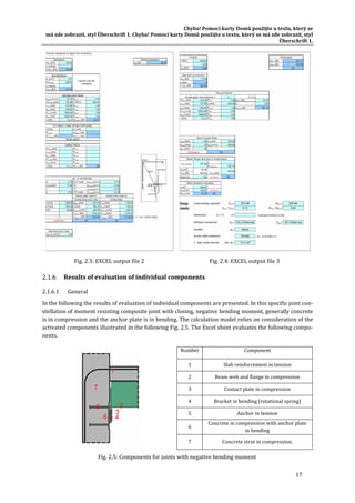

![Chyba! Pomocí karty Domů použijte u textu, který se
má zde zobrazit, styl Überschrift 1. Chyba! Pomocí karty Domů použijte u textu, který se má zde zobrazit, styl
Überschrift 1.
19
2.1.6.2 Anchor plate in compression and bending
Any result of this component is derived from the nonlinear evaluation of combined compression force from
negative bending moment and moment due to the eccentricity of shear force at the anchor plate. First the
minimum thickness required to consider the anchor plate as rigid is determined. By comparing the mini‐
mum thickness previously calculated with the actual thickness of the anchor plate, the type of the plate
under consideration is determined. If the plate is rigid, the real dimensions of the plate are used in the fol‐
lowing calculations. If flexible, an equivalent rigid and smaller plate is determined. An iterative procedure
using a macro is implemented. This macro will be started by pushing the ‘CALCULATE’ button at top sheet.
Subsequently two extreme cases are considered:
Maximum axial load under compression together with a given eccentricity moment from shear
force X eccentricity.
Maximum bending moment together with a given axial load under compression.
The given values are the same as in cells D/36 and D/33 respectively, the calculated values define the cor‐
responding forces the anchor plate configuration can bear additionally. The fictive effective size of the plate
is returned as well.
2.1.6.3 Tensional resistance of the upper row of anchors
In this part the resistance of the upper row of anchors, which possibly may be in tension, is evaluated. Dif‐
ferent failure modes are possible. Tension resistance of studs is equal to the minimum resistance value of
the five following components:
Steel failure
Steel failure is calculated according to EN 1992‐4‐2, Cl. 6.2.3 [2].
Pull‐out failure
Pull out failure is calculated according to EN 1992‐4‐2, Cl. 6.2.4 [2]. Cracked concrete is assumed, though
uncracked concrete of the wall is possible due to vertical loading in the wall; this must be separately as‐
sessed – in case the parameter may be 1,4 for uncracked concrete.
Concrete cone failure without supplementary reinforcement (modified standard model)
Cracked concrete is assumed, though uncracked concrete of the wall is possible due to vertical loading in
the wall; this must be separately assessed – in case the parameter may be 1,4 for uncracked concrete.
Concrete cone failure with supplementary hanger reinforcement
If supplementary stirrups are used with a di‐
ameter according to the input on the top sheet
and per definition with 2+2 legs, an additional
resistance component can be evaluated, as‐
suming the stirrup bar axis being 40 mm be‐
low the surface (see Fig. 2.6).This concrete
cone failure mode depends fully on the behav‐
iour of the stirrups. If steel yielding or steel
bond failure occurs before reaching the con‐
crete cone resistance, the resistance force will
be the yielding or anchorage force instead.
Yielding of stirrups
Anchoring failure of stirrups
Fig. 2.6: Definition of distance x](https://image.slidesharecdn.com/boltdesign-manualiien-191004025827/85/Bolt-design-manual-ii-en-198-320.jpg)
![Infaso+‐Handbook II
20
Splitting failure
Due to the fact, that the wall per definition is indefinite only the minimum wall thickness must be checked.
For long studs with large cones splitting is generally possible and must be assessed. The existence of a min‐
imum surface reinforcement is sufficient to avoid splitting failure. This reinforcement should be determined
in each orthogonal direction according to Eq. (2.1). The material safety factor used with reinforcement bars
is γs = 1,15. If this conditions is not fulfilled, the resistance force for splitting failure will be calculated.
A 0,5 ∙
N
f /γ ,
(2.1)
2.1.6.4 Diagonal concrete strut
Regarding the concrete part of the wall, for the bending moment a
simple single diagonal compression strut has been assumed. In Fig.
2.7this strut is represented by a dashed line.
2.1.6.5 Longitudinal steel reinforcement in tension
The longitudinal reinforcement of the concrete slab is the only ele‐
ment considered in the tension zone. Concrete is ignored. The ten‐
sion force is calculated using a two‐point‐section with reinforce‐
ment in slab and compression point in the middle of lower flange,
fulfilling equilibrium. The resistance of this first component is eval‐
uated according to EN 1994‐1‐1, Cl. 4.4 [10] and is restricted to re‐
inforcement within the effective width according to Cl. 4.2.
2.1.6.6 Shear components
In this part the shear resistance of the anchors is evaluated. Three resistance components can be deter‐
mined for shear: friction, steel failure of the anchors and pry‐out failure. Shear resistance of studs is equal
to the minimum resistance value of the three components mentioned above.
Friction
In the compressed area a friction component acting opposite to the shear force is possible. Nevertheless the
coefficient at that stage is set to zero, i.e. no friction.
Steel failure
Steel failure is calculated according to EN 1992‐4‐2, Cl. 6.3.3 [2].
Pry‐out failure
Pry‐out failure is calculated according to EN 1992‐4‐2, Cl. 6.3.4 [2].
Resulting shear resistance
The shear force which can be applied to the concrete wall is restricted by two mechanism – the minimum
of these two will be the relevant design force under given geometrical circumstances.
Pure shear: the shear resistance is derived from the fore mentioned considerations. This value
is governed under usual circumstances, as found in real structures. This force is called VRd,V.
Shear force with small eccentricity: the shear force can be limited as well by the resistance of
the anchor plate. The maximum moment derived from eccentricity under a given compression
force is evaluated in 2.1.6.2 cell D/36. Divided by the lever arm of the bracket the shear force
called VRd,M is defined.
Fig. 2.7: Strut and tie model](https://image.slidesharecdn.com/boltdesign-manualiien-191004025827/85/Bolt-design-manual-ii-en-199-320.jpg)
![Chyba! Pomocí karty Domů použijte u textu, který se
má zde zobrazit, styl Überschrift 1. Chyba! Pomocí karty Domů použijte u textu, který se má zde zobrazit, styl
Überschrift 1.
21
2.1.6.7 Other steel components
In this part other steel components on top of the anchor plate might be assessed that should not fail even if
they are not part of the model “anchor plate with headed studs”. Under consideration are: steel contact
plate, beam web and flange in compression and steel bracket. The first two are calculated using
EN 1994‐1‐1 [10] and EN 1993‐1‐8 [9], respectively. The steel bracket is analysed comparing the acting
bending moment with resisting bending moment, at the cross‐section in contact with the anchor plate. Ad‐
ditionally one must assess the welding seams of the bracket as well. The assessment of these components
is returning ‘OK’ or ‘NOT OK’. The user has to decide what actions to be taken (e.g. changing geometry or
material grades) to fulfil the requirements.
Global Results
2.1.7.1 Utilisation in terms of overall bending moment and shear
At the bottom of second sheet the load bearing capacity and utilization of the joint assemblage for tension
and shear is given in terms of VR,d and MR,d, resp VS,d/VR,d and MS,d/MR,d. These values are transferred to bot‐
tom of top sheet (see 2.1.5).
2.1.7.2 Interaction
In case of tension and shear in the stud additionally the combined action of both components must be as‐
sessed. As it is a rare situation due the governing compression force from closing moments, usually there is
no limitation. If tension and shear forces have to be considered, Eq (2.2) can be applied according to
EN 1992‐4‐2, Cl. 6.4.1 [10].
V ,
V ,
T ,
T ,
1 (2.2)
As Exponent α = 2,0 is taken in case of steel failure acc. to Cl. 6.4.1.1 or α = 1,5 in case of other failure modes
acc. to Cl. 6.4.1.2. In case of supplementary reinforcement which is designed for both failure modes tension
and shear, the same α can be applied. For simplification, and according to the current status of European
approvals for headed studs, the value α = 1,5 is used.
2.1.7.3 Stiffness and ductility
Due to the character of the joint, the stiffness of the moment resisting joint (i.e. relation of overall bending
moment to rotation) depends mainly on the nonlinear flexibility of steel/concrete bond, the slip of studs in
slab and the behaviour of concrete shear panel in the wall which is activated by the bend of reinforcement,
whereas the compression strain in the anchor plate is inferior. This approximate joint stiffness by M*lever
arm/horizontal displacement in axis of reinforcement is given with two parameters:
Sini = initial stiffness in unit [MNm/rad] gives the relation between bending moment and rotation
of the connection in the very beginning. The incline represents the maximum elastic behaviour.
Ssec = Secant stiffness in unit [MNm/rad] gives the relation between the effective bending moment
and the according, possibly nonlinear rotation of the connection. The incline is always equal (in
case of small bending moment and elastic behaviour) or typically smaller than Sini.
The term ductility is usually used in connections with energy consuming behaviour due to plasticity, if there
is displacement which will not reset but will remain in case of load removal. So even if the descent of stiff‐
ness Ssec points to nonlinearity it mostly will be a nonlinear elastic effect, which yields no ductility factor. In
that case the cell will give the information ‘elastic’.
2.1.7.4 Anchor plate and minimum tensional reinforcement
The type of anchor plate behaviour is given as information (rigid/flexible) and represents cell B45 of this
sheet and the minimum tensional reinforcement (design) in the slab is given as information.](https://image.slidesharecdn.com/boltdesign-manualiien-191004025827/85/Bolt-design-manual-ii-en-200-320.jpg)
![Infaso+‐Handbook II
22
2.2 Slim anchor plate with headed studs – bending joints
General
With the program “slim anchor plates with headed studs ‐ bending joints” (Version 2.0) [22] load carrying
capacities of joints with minimum four and maximum six headed studs can be proved. The headed studs
therefore have to be placed in two rows and the loading only can be considered in one direction (see Fig.
2.8). In the progress of the calculation the deformation behaviour of the anchor plate up to a kinematic chain
is taken into consideration. At the end a moment‐rotation curve can be obtained. The load carrying capacity
of the tensional component can be increased by taking the supplementary reinforcement which is placed
next to the headed studs into account. Compared to pure concrete cone failure the capacity of this compo‐
nent can be highly increased due to supplementary reinforcement. Within anchor plates, where the load
carrying capacity of the tensional‐, bending‐ or combined components is not governed due to failure of the
steel components (anchor plate in bending, headed studs in tension) high increases in loading of the joint
are possible. Additional the knowledge of the deformation behaviour of the joint can be used in the global
analysis.
Fig. 2.8: Geometry of the joint with slim anchor plate
Program structure and static model
2.2.2.1 General
The design software is based on the EXCEL table calculation program with the integrated programming
language VBA. Within the EXCEL file ten different spreadsheets for the in‐ and output, for the design of the
different components, for the consideration of the joint in the global analysis and for a summary of the joint
properties. Due to physical non‐linear behaviour of the anchor plate under bending forces and the geomet‐
ric non‐linear effects based on the development of cinematic chains, the design approach is done iteratively
with consideration of changes in the system. The geometric non‐linear effect occurs due to the activation of
the anchor plate due to tension forces and additional non‐linear load‐deformation behaviour of the single
components. This is implemented in the VBA‐program, which is accessing the input data from the different
spreadsheets.](https://image.slidesharecdn.com/boltdesign-manualiien-191004025827/85/Bolt-design-manual-ii-en-201-320.jpg)
![Chyba! Pomocí karty Domů použijte u textu, který se
má zde zobrazit, styl Überschrift 1. Chyba! Pomocí karty Domů použijte u textu, který se má zde zobrazit, styl
Überschrift 1.
23
2.2.2.2 Load‐transfer of the vertical loads N and the bending moment M – static model at the beginning
of the calculation process
The first model for the load transfer of the vertical loads N and the bending moments M is a continuous
beam supported on single springs. The anchor plate is therefore modeled as a two‐dimensional system. As
the connected profile stiffens the anchor plate, this sections is modeled with rigid members. Springs for
compression are placed at the nodes 1 to 8 to reflect the behaviour of the concrete under compression. If
the anchor plate is not in contact with the concrete surface and no compression forces in this place might
occur, the springs can be neglected. Non‐linear tensional springs are reflecting the load carrying behaviour
of the headed stud with the supplementary reinforcement. Depending on the geometry of the anchor plate
the tensional springs can be only placed on the nodes 2 and 7, 3 and 6 or 4 and 5. They are only activated if
the distance between the anchor plate and the concrete surfaces increases. If not a spring which is simulat‐
ing the compression forces of the concrete is placed at the same node. There are no hinges in the continuous
beam at the beginning of the calculation, but within the calculation process plastic hinges might occur at the
nodes 2, 3, 6 and 7. After each load step the boundary conditions of the supporting springs are adopted. The
prying forces of the anchor plate are considered by the compression springs in the external nodes 1 and 8
(see Fig. 2.9).
Fig. 2.9: Design model for vertical loads and bending moments
The calculation will be done by displacement method. Non‐linear (physical) effects will be considered by an
iterative calculation with continuous increase of load steps. For every load step the support conditions and
the appearance of plastic hinges will be checked. In case of changing support conditions or appearance of
plastic hinges the corresponding elements of the total stiffness matrix K, the kinematic transformation ma‐
trix a and the vector of the external nodal forces P will be manipulated. In case of bending loads without
tension forces (N ≥ 0) the row of headed studs near to the compression zone is not considered as support
spring for tension loads (cs=0). Internal forces and global node deformations caused by bending moments
and normal forces will be determined by using the displacement method, (Krätzig [18]).
v a ∙ V (2.3)
s k ∙ v ṡ (2.4)
P a ∙ s (2.5)
P a ∙ k ∙ aV a ∙ ṡ K ∙ V a ∙ ṡ (2.6)
V K ∙ P K ∙ a ∙ ṡ (2.7)
s k ∙ a ∙ V ṡ (2.8)](https://image.slidesharecdn.com/boltdesign-manualiien-191004025827/85/Bolt-design-manual-ii-en-202-320.jpg)

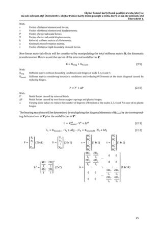
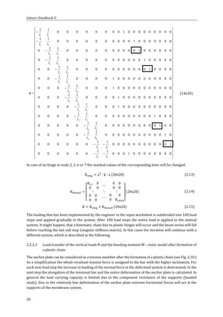

![Infaso+‐Handbook II
28
“NL_Berechnung” Iterative calculation of internal forces and bearing reactions by using the worksheet
“Calculation core anchor plate” for 100 load steps; change of support conditions or in‐
troducing plastic hinges depending of the bearing reactions or the internal forces for
the current load step; system change after reaching a kinematic structure
Components
The following components are implemented in the program. Detailed explanations of this components can
be found in Handbook I in the specific sections. The load deformation behaviour of the anchor plate is con‐
sidered within the iterative calculation of the load steps.
Tab. 2.3: Components implemented in the calculation program for slim anchor plate
Component
Headed stud
in tension
Concrete
breakout in
tension
Stirrups in ten‐
sion
Pull‐out fail‐
ure of the
headed stud
Headed stud in shear
Figure
Component Friction Concrete in compression
Threaded studs in tension/
shear
Figure
Safety factors
Tab. 2.4: Ultimate limit state (CEN/TS 1992‐4‐1:2009 4.4.3.1.1 [1])
Steel
Anchors tension Anchors shear Reinforcement
Ms Ms Ms,re
Ms=1,2*fuk/fykMs≥1,4) Ms=1,0*fuk/fyk Ms≥1,25 (fuk≤800 N/mm² and fyk/fuk≤0,8)) 1,15
Ms=1,25 (fuk>800 N/mm² or fyk/fuk>0,8)
Tab. 2.5: Ultimate limit state (EN 1993‐1‐8 [9]) Tab. 2.6: Ultimate limit state (CEN/TS 1992‐4‐
1:2009 4.4.3.1.2 [1])
Steel Concrete
Steelplate
Cone fail‐
ure
Pry‐out
failure
Pull out fail‐
ure
Anchor. fail‐
ure
Ma
Mc Mc Mp Mc
1,00
1,5 1,5 1,5 1,5
(no stability failure)
Boundary conditions
Anchor plates with headed studs at the concrete side and a welded steel profile at the airside do have com‐
plex three dimensional load transfer. Under compression forces all sections of the anchor plate are sup‐
ported in places, where a gap might occur (except in the area of the headed studs) under tensional forces.
The web and the flange of the welded steel sections do have a stiffening effect on the anchor plate. Inde‐
pendently from the thickness of the anchor plat the anchor plate is assumed in the stiffened sections as
almost completely rigid. Due to this reason the system is assumed as two dimensional continuous beam. In](https://image.slidesharecdn.com/boltdesign-manualiien-191004025827/85/Bolt-design-manual-ii-en-207-320.jpg)
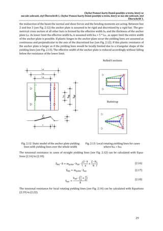

![Chyba! Pomocí karty Domů použijte u textu, který se
má zde zobrazit, styl Überschrift 1. Chyba! Pomocí karty Domů použijte u textu, který se má zde zobrazit, styl
Überschrift 1.
31
Values X and Y as small as possible
Fig. 2.15: Arrangement of the hanger reinforcement
Input mask
The input sheet “Input + Output” shows on
top a sketch of the connection labeling the
most important input parameters. In the
second part of the worksheet the dimen‐
sions, materials and loads on the anchor
plate can be entered into the program. With
the “Calculation‐Button” on the right bot‐
tom of the worksheet the non‐linear deter‐
mination of internal forces and the compo‐
nent design will be started. Left beside the
“Calculation‐Button” the degree of utiliza‐
tion of the main components is shown. In
the following the input data is described in
particular.
Steel profile (1. line): Input of the length
lPR [mm] and the width bPR [mm] of the con‐
nected profile or steel element to deter‐
mine the rigid plate area. In case of connec‐
tions of steel profiles with head plates by
threaded studs welded on the anchor plate
directly the outer distances of the threaded
studs in both directions have to be used for
lPR and bPR.
Anchor plate (2. line): Input of the length
lAP [mm], the width bAP [mm] and the thick‐
ness tAP [mm] of the anchor plate; the num‐
ber of headed studs per row (2 or 3); the
material of the steel plate (acc. to EN 1993‐
1‐1 Chyba! Nenalezen zdroj odkazů. and
EN 10025 [4]).
Headed studs (3. line): Input of the dis‐
tances of the headed studs in longitudinal direction lHS [mm], in cross direction bHS [mm]; the shaft diameter
[mm]; the length of the studs hn [mm]; the material of the headed studs (acc. to EN 10025 and EN 10088).
In case of lHS ≤ lPR the distance bHS of the headed studs has to be equal or smaller than the width bPR plus five
times tAP (bHS≤bPR+5*tAP).
Fig. 2.16: Excel worksheet “Input + Output” page 1/1](https://image.slidesharecdn.com/boltdesign-manualiien-191004025827/85/Bolt-design-manual-ii-en-210-320.jpg)
![Infaso+‐Handbook II
32
Reinforcement (4. line): Input of the diameter dS [mm] and the material (acc. to DIN 488 [3]) of the rein‐
forcement stirrups. The reinforcement stirrups have to be formed as loops with the smallest admissible
bending role diameter. They have to be grouped in pairs close to the shafts of the headed studs with mini‐
mum distance to the bottom side of the anchor plate (maximum possible overlapping length of stirrup leg
and headed stud).
Concrete member (5. line): Input of the thickness hC [mm] and the material type (acc. to EN 1992‐1‐1 [7])
of the concrete member.
Loads (last line): Input of the bending moment MEd [kNm], the normal force NEd [kN] and the shear force
VEd [kN] as design loads (ultimate limit state). Design loads have to be determined by the user. Partial factors
will not be considered at the load side by the program!](https://image.slidesharecdn.com/boltdesign-manualiien-191004025827/85/Bolt-design-manual-ii-en-211-320.jpg)
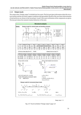
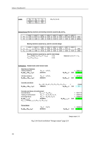
![Chyba! Pomocí karty Domů použijte u textu, který se
má zde zobrazit, styl Überschrift 1. Chyba! Pomocí karty Domů použijte u textu, který se má zde zobrazit, styl
Überschrift 1.
37
2.3 Rigid anchor plate with headed studs – simple joint
General
With the program “Rigid anchor plate
with headed studs – simple joint” (Ver‐
sion 2.0) [23] the load carrying capaci‐
ties of anchor plates with minimum four
and maximum six headed studs in two
rows under loading in one direction can
be calculated (see Fig. 2.20). It is re‐
quired, that the point of load transfer
into the simple joint is defined in the
static system as hinged. As this point
can`t be assumed directly located at the
concrete surface, the eccentricity has to
be taken into consideration. As the
shear load is applied with some eccen‐
tricity also bending moments in the an‐
chor plate have to be considered beside
normal and shear forces. In order to in‐
crease the tensional resistance of the
component of the headed stud, supple‐
mentary reinforcement can be used next to the studs. With the supplementary reinforcement high increases
in loading of the joint are possible as the load carrying capacity of pure concrete cone failure can be in‐
creased by taking the reinforcement into account. The anchor plate is assumed to be rigid without any plas‐
tic reserves.
Program structure and static model
The design software is based on the EXCEL table calculation program with the integrated programming
language VBA. Within the EXCEL file ten different spreadsheets for the in‐ and output, for the design of the
different components, for the consideration of the joint in the global analysis and for a summary of the joint
properties. In a first step the height of the compression zone is assumed. Based on this assumption all un‐
known forces in Fig. 4.11 can be calculated. Based on moment equilibrium and equilibrium in the vertical
direction the assumption can be verified. The shear force VEd is carried by a frictional part and the two shear
components of the headed studs, see Eq. (2.24) .
V V , V , V (2.24)
With the equilibrium of moments at the intersection point of the action lines of the concrete force CEd and
the shear components of the headed studs VEd,2 and VEd,1 the formulations in Eq. (2.25) can be obtained for
the calculation of the applied normal force in the second stud row. By a vertical equilibrium of forces the
assumed height of the compression zone can be verified. In the program the effective compressive height is
determined iteratively. For further information see Design Manual I "Design of steel‐to‐concrete joints",
Chapter 5.2.2 [13] and for the calculation of the deformations see Chapter 4.2 and Chapter 4.3.
V V , ∙
e t d
z μ ∙ d
(2.25)
EXCEL Worksheets / VBA program
The whole design tool contains 10 Microsoft Excel worksheets. Visible for the user are only the worksheets
“Input + Output CM” and “Design output CM”. The following schedule gives a short overview about the func‐
tion of the different worksheets (see Tab. 2.8).
Fig. 2.20: Geometry of the joint with rigid anchor plate](https://image.slidesharecdn.com/boltdesign-manualiien-191004025827/85/Bolt-design-manual-ii-en-216-320.jpg)
![Chyba! Pomocí karty Domů použijte u textu, který se
má zde zobrazit, styl Überschrift 1. Chyba! Pomocí karty Domů použijte u textu, který se má zde zobrazit, styl
Überschrift 1.
39
Boundary condition
The calculation of the design resistance of the connection between the steel element and the anchor plate
is not covered by the program and has to be done separately by the engineer. If the steel elements or the
steel profiles are not directly welded to the anchor plate and connected by threaded studs and an endplate
the dimensions lAP and bAP have to be defined analogous independent from the actual dimensions of the
steel profile (for example with the distances of the threaded studs lAP and bAP). The new components that
are used in the program are based on test with large edge distances of the headed studs. Due to this reason
the edge distances described in Chapter 2.2.6 are required. Also requirements for the exact location of the
supplementary reinforcement are given there.
Input mask
The input sheet “Input + Output” shows on
top a sketch of the connection labeling the
most important input parameters (see Fig.
2.21). In the second part of the worksheet
the dimensions, materials and loads on the
anchor plate can be fed into the program.
With the “Calculation‐Button” on the right
bottom of the worksheet the determination
of internal forces and the component de‐
sign will be started. Left beside the “Calcu‐
lation‐Button” the degree of utilization of
the main components is shown. In the fol‐
lowing the input data is described in partic‐
ular.
Steel profile (1. line): Input of the length
lPR [mm] and the width bPR [mm] of the con‐
nected butt strap.
Anchor plate (2. line):Input of the length
lAP [mm], the width bAP [mm] and the thick‐
ness tAP [mm] of the anchor plate; the num‐
ber of headed studs per row (2 or 3); the
material of the steel plate (acc. to EN 1993‐
1‐1 [8] and EN 10025 [4]).
Headed studs (3. line):Input of the dis‐
tances of the headed studs in longitudinal
direction lHS [mm], in cross direction bHS
[mm]; the shaft diameter [mm]; the length
of the studs hn [mm]; the material of the
headed studs (acc. to EN 10025 [4]).
Reinforcement (4. line): Input of the diameter dS [mm] and the material (acc. to DIN 488 [3]) of the rein‐
forcement stirrups. The reinforcement stirrups have to be formed as loops with the smallest admissible
bending role diameter. They have to be grouped in pairs close to the shafts of the headed studs with mini‐
mum distance to the bottom side of the anchor plate (maximum possible overlapping length of stirrup leg
and headed stud).
Concrete member (5. line): Input of the thickness hC [mm] and the material type (acc. to EN 1992‐1‐1 [7])
of the concrete member.
Fig. 2.21: Excel worksheet “Input + Output CM” page 1/1](https://image.slidesharecdn.com/boltdesign-manualiien-191004025827/85/Bolt-design-manual-ii-en-218-320.jpg)
![Infaso+‐Handbook II
40
Loads (last line): Input of the shear force VEd [kN] and their eccentricity to the anchor plates surface in
[cm]. Design loads have to be determined by the user. Partial factors will not be considered at the load side
by the program!
Output mask
The output sheet “Design output” is divided into three parts. The first part gives information about the
structural system (see Fig. 2.21). Results of the static calculation of internal forces are shown in the second
part (see Fig. 2.23). In part 3 the main verifications of the components are given (see Fig. 2.23).
Fig. 2.22: Excel worksheet “Design output CM”
page 1/2
Fig. 2.23: Excel worksheet “Design output CM”
page 2/2
Optimization of the joint
The optimization of the joint can be done according to the optimization of the connection of the slim anchor
plate (see Chapter 2.2.9) more information about optimization of simple joints is given in the parameter
study for simple joints in Chapter 4.3.](https://image.slidesharecdn.com/boltdesign-manualiien-191004025827/85/Bolt-design-manual-ii-en-219-320.jpg)

![Infaso+‐Handbook II
42
3 Design examples
3.1 Composite beam of a standard office structure connected to reinforced con‐
crete wall
General
3.1.1.1 Depiction of the situation
Multistory office building structures often
have a floor modulus of n ∙ 1,35 m by approx.
7,8 m, which results from the room depth
plus corridor. Beneath several variation of
concrete slabs with or without beams con‐
crete steel composite beams made of a hot
rolled cross section IPE 300 with a semi‐fin‐
ished concrete slab connected by studs can
be used to reduce the height of the construc‐
tion and by this means the total height of
each floor. One possibility to design a con‐
struction of minimum height properly can be
the moment resistant constraint in the wall.
The knowledge of rotational behaviour of the
connection allows to optimize the connec‐
tion on behalf of reinforcement and to evalu‐
ate the redistribution of forces.
3.1.1.2 Overall structural system
The example shows a concrete steel composite beam made of a hot rolled cross section IPE 300 with a semi‐
finished concrete slab (total 14 cm) connected by studs. The lateral distance of the beams is 2 ∙ 1,35 m
2,70m, the span is 7,8 m. The inner support can be at a reinforced concrete (RC) wall of the building core,
the outer support is a façade column (see Fig. 3.1).
Semi‐finished slab (6cm precast concrete) + cast in‐situ of altogether 14 cm, continuous system,
span 2,70 m each.
Hot rolled beam IPE 300 S355 JR, L = 7,8 m; uniformly distributed loading with headed studs.
Support façade: Steel column spaced 2,7 m.
Support inner core: Reinforced concrete wall with fully restraint connection by reinforcement and
steel/concrete compression contact.
3.1.1.3 Loads
Own weight slab g’ = 1,6 kN/m
Own weight slab g1 = 3,5 kN/m²
Dead load screed g2 = 1,6 kN/m
Dead load suspended ceiling + installation g3 = 0,4 kN/m²
Dead load (total) g = 5,50 kN/m²
Live load (B2,C1 acc. DIN 1991‐1‐1 NA [5]) q = 3,00 kN/m²
Fig. 3.1: Structural system](https://image.slidesharecdn.com/boltdesign-manualiien-191004025827/85/Bolt-design-manual-ii-en-221-320.jpg)
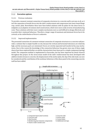
![Infaso+‐Handbook II
44
Fig. 3.2: Geometry of the composite joint
Structural analysis of the joint
3.1.3.1 Modelling
The member forces of the structure generally can be calculated with any software which is able to consider
ranges of different beam stiffness and rotational springs. As the structure is statically indeterminate the
different stiffness of the positive and negative moment range must be taken into account to properly calcu‐
late the member and support forces. For this example the software KRASTA [21] for spatial frame analysis
has been used. Prior to any calculation we can do a reliable prediction concerning the quality of moment
distribution. There will be a maximum negative moment at the moment resistant support, the moment will
then be reduced and will cross the zero‐line. Afterwards it will drop down to its positive maximum at ap‐
prox. 5/8 of the span and ending at zero at the hinged support at the end of the beam. The negative range is
assumed for the first quarter of span, the positive is set for the rest of span. According to EN 1994‐1‐1
Cl. 5.4.1.2 [10] the effective width can be calculated with Eq. (3.1).
b b b , (3.1)
In case of equally spaced beams these equation can be calculated in the negative range with Eq. (3.2) and in
the positive range with Eq. (3.3) each of them less as the spacing between adjacent beams (270 cm). This
means that necessary reinforcement bars in the negative range of the slab must be arranged within the
effective width.
b , 15 2 ∙ 780 ∙ 0,25/8 63,8 cm (3.2)
b , 15 2 ∙ 780 ∙ 0,75/8 161,25 cm (3.3)
The different moments of inertia Ipos are calculated in accordance to common values of creep influence (see
Eq. (3.4) to (3.5). In this example the relation between stiffness shortly after erection and after 1‐2 years
(means T=∞) is approximately ¾. The effect of shrinking (eccentricity of tensional force in slab) is not con‐
sidered. The moment of inertia for T=∞ will be used with dead load and value for T=0 will be used with life
load. This will yield the maximum restraint moment and force at support A.
Negative range: I 18360 15,5 ∙ 30/2 15 4 ² 18000 cm (3.4)
Positive range: Ipos, t=0 ≈ 30200 cm4 Ipos, t=∞ ≈ 22500 cm4 (3.5)
3.1.3.2 Calculation of forces
Using the previous mentioned
characteristics in the first iteration
of forces, the rotation stiffness of
the connection is set to infinite, i.e.
complete moment resistant re‐
straint. The resultant internal
forces for characteristic points of
the beam are shown in Fig. 3.3.
The next step will be an assess‐
ment of the moment restraint con‐
nection and the evaluation of rota‐
tion to define a rotational spring
characteristic.
Fig. 3.3: Mind: these are independently calculated input values for](https://image.slidesharecdn.com/boltdesign-manualiien-191004025827/85/Bolt-design-manual-ii-en-223-320.jpg)
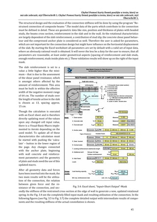
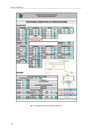
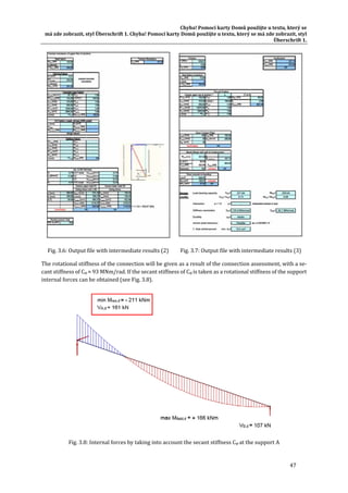


![Infaso+‐Handbook II
50
3.2 Column base as connection of a safety fence on a car parking deck to a rein‐
forced concrete slab
General
3.2.1.1 Depiction of the situation
A safety fence, consisting of a horizontal beam barrier of two connected hollow sections on vertical
columns of rolled sections, is connected at the column bases to a 300 mm thick reinforced concrete
slab. Embedded anchor plates with headed studs and welded threaded studs are used to connect
the columns base plates with the concrete deck. The distance between the steel columns varies
from 1,50 m up to 2,00 m and the centre of the beam barrier is 0,50 m above the concrete surface.
The whole construction has to be protected against corrosion, for example by galvanization.
3.2.1.2 Overall structural system
Horizontal beam barrier:
Single span beam L = 1,50 m up to 2,00 m; loaded by a horizontal vehicle impact force.
Vertical column:
Cantilever beam (vertical) L = 0,50 m; loaded by a horizontal vehicle impact force (directly or indirectly by the beam
barrier)
3.2.1.3 Loads
Impact passenger car (EN 1991‐1‐7, Cl. 4.3.1 [6]) Fdx = 50,00 kN
(Load application 0,50 m above street surface)
3.2.1.4 Joint loads
Design load VEd = Fdx = 50,00 kN
MEd = 50,00 * 0,50 = 25,00 kNm
Execution options
3.2.2.1 Previous realization
Fig. 3.10: Conventional joint solution of the safety fence](https://image.slidesharecdn.com/boltdesign-manualiien-191004025827/85/Bolt-design-manual-ii-en-229-320.jpg)
![Chyba! Pomocí karty Domů použijte u textu, který se
má zde zobrazit, styl Überschrift 1. Chyba! Pomocí karty Domů použijte u textu, který se má zde zobrazit, styl
Überschrift 1.
51
In the conventional joint solution the columns base plate is directly bolted to the anchor plate by threaded
studs which are welded on the embedded steel plate (see Fig. 3.10). In order to reduce the headed studs
tension forces caused by bending, the distance of the studs in load direction and therewith the length of the
embedded steel plate have to be large. For this reason the distance between the threaded bolts and headed
studs is quite large and high bending moments in the anchor plate are resulting. The anchor plates is de‐
signed as thick and rigid in order to consider an elastic approach in the calculation. The dimensions of the
anchor plate are given in the following.
Base plate 200 / 200 / 20 mm S 235
Threaded bolts ø 20 mm fub = 500 N/mm²
Distance threaded bolts 150 / 150 mm
Anchor plate 350 / 350 / 30 mm
Headed studs 22 / 175 mm S 235
Distance headed studs 270 / 270 mm
3.2.2.2 Improved realization Version 1
Fig. 3.11: Improved realization Version 1
Within this modified joint solution the new components of the INFASO [12] project are considered. In this
solution the columns base plate is directly bolted to the anchor plate by threaded studs which are welded
on the embedded steel plate (see Fig. 3.11). The choice of a quite small anchor plate generates high tension
forces in the headed studs caused by external bending moment. So additional hanger reinforcement is fixed
very close to the headed studs loaded by tension forces. The distance of the headed studs in load direction
is small. Due to the fact that the headed studs and the threaded studs are spaced very close, low bending
moments in the anchor plate are resulting. A plastic design of the anchor plate is possible. Thin steel plates
can be used. The complete embedded plate is covered by the columns base plate. The dimensions of the
anchor plate are given in the following.
Base plate 200 / 200 / 20 mm S 235
Threaded bolts ø 20 mm fub = 500 N/mm²
Distance threaded bolts 150 / 150 mm
Anchor plate 200 / 200 / 12 mm
Headed studs 22 / 175 mm S 235
Distance headed studs 150 / 150 mm](https://image.slidesharecdn.com/boltdesign-manualiien-191004025827/85/Bolt-design-manual-ii-en-230-320.jpg)
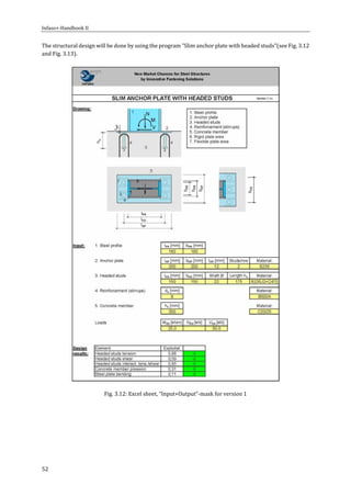
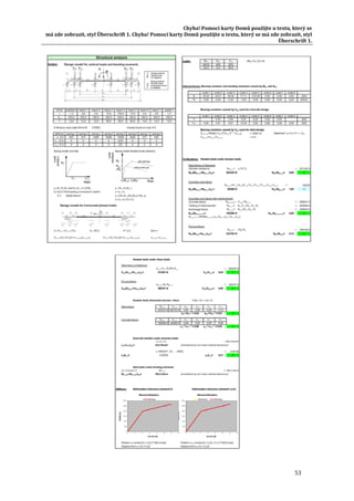
![Infaso+‐Handbook II
54
Fig. 3.13: Excel sheet, “Design output” for version 1
3.2.2.3 Improved realization‐Version 2
Description of a modified joint solution considering
the new components of WP 1
Within this modified joint solution the new components
of the INFASO [12] project are considered. The columns
base plate is directly bolted to the anchor plate by
threaded studs which are welded on the embedded
steel plate. Except that the anchor plate has only a thick‐
ness of 12 mm the construction is the same as shown by
structure of the previous realization. The embedded
steel plate cannot take the total bending moment. The
behaviour of the joint is comparable with a kind of plas‐
tic hinge. The joint will be designed by transformation
of kinetic energy into plastic deformation energy. The
dimensions of the anchor plate are given in the follow‐
ing.
Base plate 200 / 200 / 20 mm S 235
Threaded bolts ø 20 mm fub = 500 N/mm²
Distance threaded bolts 150 / 150 mm
Anchor plate 350 / 350 / 12 mm
Headed studs 22 / 175 mm S 235
Distance headed studs 270 / 270 mm
Fig. 3.14: Improved Version 2
For structural design information about the
bending moment resistance and the defor‐
mation behaviour of the joint is needed. The
bending moment resistance will be obtained by
using the program “Slim anchor plate with
headed studs” with stepwise increase of the ex‐
ternal forces (see Chapter 2.3). After the last
step the moment‐rotation curve of the sheet
“Design output” can be used (see Fig. 3.15). The
verification will be done according to EN 1991‐
1‐7 Annex C 2.2 [6].](https://image.slidesharecdn.com/boltdesign-manualiien-191004025827/85/Bolt-design-manual-ii-en-233-320.jpg)
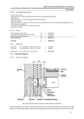

![Infaso+‐Handbook II
62
4 Parameter studies
4.1 General
In this parameter studies the three steel‐to‐concrete connections of the Design Manual I "Design of steel‐to‐
concrete joints" [13] are under examination (see Fig. 1.1). In the parameter study for concrete components
in Chapter 4.2 experimentally determined pre‐factors are taken into consideration. Their influence on the
stiffness of the concrete component is shown. In Chapter 4.3 parameters for geometry and material are
changed in order to show their influence on the load‐deformation and moment rotational behavior of the
simple steel‐to‐concrete joints. Changes in the thickness of the anchor plate and in steel grade for column
bases are explained in Chapter 4.4 where especially this two parameters have a high influence on the struc‐
tural behavior for this type of connection. Also recommendations for design values are given in this Chapter.
In the last parameter study the focus is on composite joints in Chapter 4.5.
4.2 Parameter study on concrete components
General
As discussed in Chapter 3 on concrete components in the Design Manual I "Design of steel‐to‐concrete
joints" [13], the stiffness of an anchorage group is determined by several parameters. Out of these parame‐
ters, certain parameters are known with high degree of confidence at the time of analysis such as dimen‐
sions of studs, dimensions of reinforcement and further parameters. Certain other parameters, such as con‐
crete material properties, bond strength etc. are known within the statistical range of distribution normally
occurring in practice. Certain parameters are used to define the stiffness and are based on empirical studies,
which are not known with a high certainty. In this chapter, the sensitivity of the stiffness values towards
different parameters has been investigated.
Example considered
A basic example of a single headed stud with supplementary reinforcement subjected to tensile loads is
considered in this parameter study. The stud is considered to be far from the edges. All the components are
considered while evaluating the stiffness of the anchor. The variation of secant stiffness as a function of
anchor displacement is evaluated and plotted. Though the plots are given in terms of absolute values for the
anchor stiffness and displacement, the objective of this study is to relatively compare the stiffness variation
and verify, principally, the influence of different parameters.
Parameter studied and methodology followed
The stiffness of the anchorage system as a function of anchor displacement was evaluated using the formu‐
lations given in Chapter 3 of the Design Manual I "Design of steel‐to‐concrete joints" [13] and a parameter
study was performed to investigate the influence of various parameters on the stiffness of the system. While
evaluating the influence of a given parameter, all other parameters were kept constant. These parameters
are considered as independent and uncorrelated for this study. The parameters considered for the param‐
eter study along with the range of study are tabulated in Tab. 4.1. This assumption of no correlation between
the parameters is valid for all the parameters except the concrete compressive strength and the bond
strength between concrete and reinforcement. Therefore, for these two parameters, the dependence of
bond strength on concrete compressive strength is considered in this study. As can be seen from Tab. 4.1, a
sufficiently wide range is considered for the parameter studies.](https://image.slidesharecdn.com/boltdesign-manualiien-191004025827/85/Bolt-design-manual-ii-en-241-320.jpg)
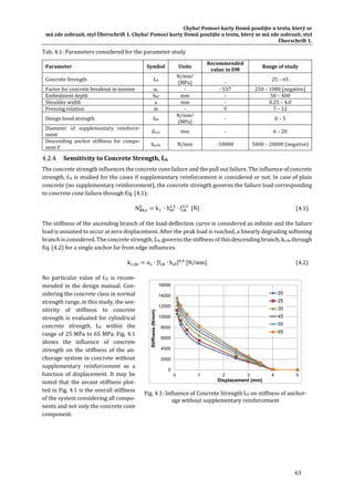


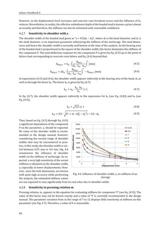
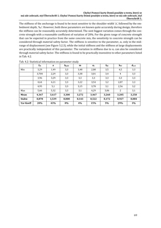
![Infaso+‐Handbook II
70
4.3 Parameter study on simple steel‐to‐concrete joints
General
The following parameter study is carried out in order to describe the influence by varying different input
factors of the simple joint. With the variation of different parameters the load bearing capacity and the ro‐
tational stiffness of the whole joint can be influenced to a high extend. The optimization of the simple joint
will be aimed to achieve on one hand maximum strength with minimum costs and on the other hand a duc‐
tile behaviour of the whole joint. For the concrete component ductility exists if the load can be transferred
at the cracked level to other components such as stirrups, as a certain amount of deformation occurs at the
maximum level of load. Furthermore the parameter study will demonstrate a range of validity and will point
out the possible increase in loading of the joint by changing different parameters.
Validation of the model
Within the INFASO project a design approach based on the component method has been developed for the
simple steel‐to‐concrete joints [12]. Thereby the joint is subdivided into its different components and the
deformations can be calculated as each of the component is represented by a spring. The calculation of the
load carrying capacity mainly consists of the following procedure:
1. Evaluation of the decisive tension component.
2. Verification of the influence of the compression zone on the tension component.
3. Calculation of the shear resistance of the joint out of the moment equilibrium, see Fig. 4.11.
4. Verification of interaction conditions.
In the Design Manual I "Design of steel‐to‐concrete joints" [13] this approach is described in more detail
based on a flowchart and a worked example. In order to determine the moment‐rotation curve of the joint,
the deformation of the single components have to be calculated. Therefore load‐deformation curves of the
single steel and concrete components have been developed. A parameter study on the concrete components
and a detailed investigation on the unknown factors of the concrete components can be found in the previ‐
ous chapter. Fig. 4.11 shows the mechanical model and a simplified joint model if the tensional and the
compression components are assembled in one spring.
The deformation of the tensional component can be determined in three ranges (see Fig. 4.11). In the first
range the deformations can be calculated according to [12] with Eq. (4.12). For this the deformation due to
pull‐out failure (see Eq. (4.5)) and the deformation due to elongation of the shaft of the headed stud are
added.
δ δ , , δ , (4.12)
With:
δ , , Deformation due to pull‐out failure;
δ , Deformation due to yielding of the headed stud.
Fig. 4.11: Analytic model of the simple steel‐to‐concrete joint (left), load‐deformation of the tensional
component if supplementary reinforcement can be activated in best case (right)](https://image.slidesharecdn.com/boltdesign-manualiien-191004025827/85/Bolt-design-manual-ii-en-249-320.jpg)
![Chyba! Pomocí karty Domů použijte u textu, který se
má zde zobrazit, styl Überschrift 1. Chyba! Pomocí karty Domů použijte u textu, který se má zde zobrazit, styl
Überschrift 1.
71
At the end of the first range first cracks might develop from the head of the headed stud into the direction
of the concrete surface. If the load carrying capacity at concrete cone failure is reached, the supplementary
reinforcement can be activated. In this case the deformations can be calculated up to the ultimate load with
Eq. (4.13).
δ δ , , δ , δ , (4.13)
With:
δ , , Deformation due to pull‐out failure;
δ , Deformation due to yielding of the headed stud;
δ , Deformation of the supplementary reinforcement in interaction with concrete cone failure.
The deformations in the third range depend on the failure mode of the ultimate load. If yielding of the sup‐
plementary reinforcement occurs, a ductile behaviour can be observed in the third range. The deformations
in the third range can be calculated with Eq. (4.14).
δ δ N ,
N N ,
k ,
k (4.14)
With:
k , Stiffness of the descending branch see Eq. (4.2);
k
10000
If yielding of the supplementary reinforcement occurs;
k 0 If the failure mode concrete failure and anchorage failure of the stirrups occurs;
N ,
Characteristic load carrying capacity of the supplementary reinforcement in interaction
with concrete cone failure;
Ultimate load carrying capacity.
It has to be considered, that the supplementary reinforcement can only be activated in the optimum case.
As the failure modes like, pull‐out failure of the headed studs, concrete cone failure between the supple‐
mentary reinforcement and steel failure of the headed stud can also occur, scenario distinctions have to be
made in all ranges. Within the following parameter study this issue will be highlighted and explained. The
rotation of the joint can be determined with Eq. (4.15) according to the spring model of Fig. 4.12.
Φ
δ δ
(4.15)
With:
δ Deformation of the tensional component;
δ Deformation of the compression component according to Design
Manual I “Design of steel‐to‐concrete joints” [13] Eq. (3.75).
For the calculation of the full moment‐rotation curve of the joint the interac‐
tion conditions for steel failure (see Eq. (4.16)) and for concrete failure (see
Eq. (4.17)) have to be considered as tension forces and shear forces are acting
simultaneously on the simple steel‐to‐concrete joint.
Steel failure
N
N , ,
V
V , ,
1 (4.16)
Concrete failure
N
N ,
/
V
V ,
/
1 (4.17)
With:
N , , /V , , Characteristic load carrying capacity due to steel‐failure of the headed stud;
N , /V , Characteristic load carrying capacity due to concrete failure modes.
In Fig. 4.13 the validation of the model is shown for the different test specimens [12]. In this figures the
moment‐rotation curves are compared with the calculated curves according to the developed mechanical
joint model. It can be seen, that the model curves fit well to the test curves.
Fig. 4.12: Spring model](https://image.slidesharecdn.com/boltdesign-manualiien-191004025827/85/Bolt-design-manual-ii-en-250-320.jpg)
![Infaso+‐Handbook II
72
Within the first section the moment‐rotational behaviour of the joint is described up to concrete cone fail‐
ure. Test specimens without additional reinforcement reach their ultimate resistance up to this point. If
additional reinforcement is placed next to the stirrups, the load carrying capacity of the tensional compo‐
nent can be increased (see 2nd range for B1‐B‐R and B2‐C‐R in Fig. 4.13). In these cases the additional rein‐
forcement is activated and the ultimate load can be increased. In the following parameter study configura‐
tions will be shown, where the supplementary reinforcement can be activated and a ductile failure mode
can be obtained.
Sensitivity study of major parameters
4.3.3.1 General
Based on the worked example on simple joints of Design Manual I "Design of steel‐to‐concrete joints" [13]
the different parameters were defined and varied in particular in the following. The worked example is used
thereby as reference version. Safety factors weren`t considered in this parameter study. Furthermore the
absolute terms in the equations for pull‐out failure and concrete cone failure were assumed as 12 and 15.5
to reproduce the real load‐carrying capacity. Values for application may be taken from the relevant Euro‐
pean Technical Specification of the specific headed studs.
4.3.3.2 Overview of the major parameters
The load‐carrying capacity and the rotational stiffness depends on different parameters and boundary con‐
ditions. The examined parameters are listed in Table 4.1.
Moment‐rotation‐curve for test B1‐BS Moment‐rotation‐curve for test B1‐B‐R
Moment‐rotation‐curve for test R1‐C Moment‐rotation‐curve for test B2‐C‐R
Fig. 4.13: Validation of the INFASO model without supplementary reinforcement (left),
with supplementary reinforcement (right)](https://image.slidesharecdn.com/boltdesign-manualiien-191004025827/85/Bolt-design-manual-ii-en-251-320.jpg)
![Chyba! Pomocí karty Domů použijte u textu, který se
má zde zobrazit, styl Überschrift 1. Chyba! Pomocí karty Domů použijte u textu, který se má zde zobrazit, styl
Überschrift 1.
73
Tab. 4.3: Overview of the examined parameters and their influence on the model
Parameter Influence Remarks and brief description Chapter
Effective height ++
Influences the ultimate load carrying capacity as well as
the load carrying capacity of the concrete cone failure NRk,c
4.3.3.3
Eccentricity ++
Can have high influence on the moment resistance of the
joint within high utilization factors of the interaction equa‐
tions
4.3.3.5
Diameter headed studs +++ High influence on the ductility of the joint. 4.3.3.3
Diameter stirrups ++
Diameter of the stirrups can increase the overall load‐car‐
rying capacity
4.3.3.6
Number of stirrups ++
If the number of stirrups is increases brittle failure modes
can be avoided.
4.3.3.6
Concrete strength +++
Concrete strength has influence on all concrete compo‐
nents
4.3.3.7
4.3.3.3 Effective height
The effective height (see Fig. 4.4) can either be varied by changing the thickness of the anchor plate, the
overall length of the headed stud or the head height of the anchor. In this study only the anchor length has
been modified as this factor has the biggest influence on the final result, see Tab. 4.4.
Tab. 4.4: Analyzed effective heights
Parameter Case 1 Case 2
Reference ver‐
sion
Case 3 Case 4
Anchor length [mm] 50 100 150 200 250
Effective height [mm] 65 115 165 215 265
Fig. 4.14 shows the load‐displacement curve of the tensile component. The desired behaviour of the simple
joint can be monitored, if an effective height of 165 mm is used. By selecting this effective height all three
sections δRange1, δRange2 and δRange3 in Fig. 4.14 are clearly evident. By the end of the first section δRange1 the
ultimate load of the concrete cone failure without considering supplementary reinforcement NRk,c = 190 kN
is reached for the reference version (see Tab. 4.4). By further increase of the load, the hanger reinforcement
is activated and the smallest resistance of steel yielding of the stirrups NRk,re,1, anchorage failure of the stir‐
rups NRk,re,2 or the small concrete cone failure NRk,cs can be decisive. In the third range δRange3 the inclination
of the load‐displacement‐curve depends whether brittle failure modes like concrete cone failure or anchor‐
age failure or steel failure becomes crucial. According to Fig. 4.14 ductile behaviour occurs if longer headed
studs are used. The headed stud is yielding before other failure modes can be recognized. Fig. 4.14 indicates
that the selection of longer headed studs does not increase the load carrying capacity of the tensional com‐
ponent of the joint. In this cases steel failure of the headed studs becomes the decisive failure mode. If
headed studs with smaller effective heights are used, brittle failure modes might occur. For effective height
of 115 mm concrete cone failure between the supplementary reinforcement with approx. NRk,cs = 250 kN is
decisive and for an effective height of 65 mm with approx. NRk,cs = 105 kN is the governing failure mode. In
Fig. 4.15 the moment‐rotation curve by varying the effective length of the headed stud is shown. By changing
the effective height the rotational behavior of the joint can be influenced less as if the diameter of the heads
stud is changed. Changes of the diameter of the headed stud have higher influence on the stiffness EA of this
component (see Eq.(4.12)).](https://image.slidesharecdn.com/boltdesign-manualiien-191004025827/85/Bolt-design-manual-ii-en-252-320.jpg)
![Infaso+‐Handbook II
74
4.3.3.4 Diameter of the headed studs
In Fig. 4.16 the load‐displacement curves of the tensional component for different diameters of the headed
stud is shown. The diameters of the headed studs are varied according to Tab. 4.5. By using a diameter of
22 mm in the reference version the supplementary reinforcement can be activated. This can be seen in Fig.
4.16 as the load can be increased from approx. NRk,u,c = 190 kN up to NRk,u = 350 kN (for definition see Fig.
4.11, right). The overall load carrying capacity cannot be increased by selecting even a higher diameter of
the headed stud. As yielding of the supplementary reinforcement becomes the decisive component with
NRk,re,1 = 350 kN a larger diameter is not more advantageous. If the diameter is reduced, the increase in
Fig. 4.14: Load‐displacement curve of the tensional component for variation of the effective height
Fig. 4.15: Moment‐rotation curve for variation of the effective height
0
50
100
150
200
250
300
350
400
0,00 0,50 1,00 1,50 2,00 2,50 3,00 3,50 4,00 4,50 5,00
Load[kN]
Displacement [mm]
Load-displacement curve
hn = 50 mm
hn = 100 mm
hn = 150 mm
hn = 200 mm
hn = 250 mm
0,00
0,20
0,40
0,60
0,80
1,00
1,20
0,00 1,00 2,00 3,00 4,00 5,00 6,00 7,00 8,00 9,00 10,00
Mref/Mx[-]
Rotation [mrad]
Moment-rotation curve
hn = 50 mm
hn = 100 mm
hn = 150 mm
hn = 200 mm
hn = 250 mm](https://image.slidesharecdn.com/boltdesign-manualiien-191004025827/85/Bolt-design-manual-ii-en-253-320.jpg)
![Chyba! Pomocí karty Domů použijte u textu, který se
má zde zobrazit, styl Überschrift 1. Chyba! Pomocí karty Domů použijte u textu, který se má zde zobrazit, styl
Überschrift 1.
75
loading due to the supplementary reinforcement cannot be taken into account fully. In this case a diameter
of 16 mm is too small as the load level of concrete cone failure, NRk,c = 190 kN, cannot be reached. In Fig.
4.17 the moment‐rotation curves of this simple steel‐to‐concrete joint by varying the diameter of the headed
stud are shown. The variation of the diameter has also an influence on the interaction equations of the joint.
Steel failure might become the decisive interaction equation.
Tab. 4.5: Diameter of the headed studs
Parameter Case 1 Case 2 Case 3 Reference version Case 4
Diameter headed studs
[mm]
13 16 19 22 25
Fig. 4.16: Load‐displacement curve of the tensional component for variation of the diameter of the
headed studs
Fig. 4.17: Moment‐rotation curve of the simple steel‐to‐concrete joint for variation of the diameter of
the headed studs
0
50
100
150
200
250
300
350
400
0,00 2,00 4,00 6,00 8,00 10,00 12,00 14,00 16,00 18,00 20,00
Load[kN]
Displacement [mm]
Load-displacement curve
ds,nom = 16 mm
ds,nom = 19 mm
ds,nom = 22 mm
ds,nom = 25 mm
0,00
0,20
0,40
0,60
0,80
1,00
1,20
1,40
0,00 10,00 20,00 30,00 40,00 50,00 60,00 70,00 80,00 90,00 100,00
Mref/Mx[-]
Rotaition [mrad]
Moment-rotation curve
ds,nom = 16 mm
ds,nom = 19 mm
ds,nom = 22 mm
ds,nom = 25 mm](https://image.slidesharecdn.com/boltdesign-manualiien-191004025827/85/Bolt-design-manual-ii-en-254-320.jpg)
![Infaso+‐Handbook II
76
4.3.3.5 Eccentricity
According to Tab. 4.6 five different cases are considered in order to determine the influence of the eccen‐
tricity on the rotational behavior of the joint. Originally there shouldn`t be any effect to the load‐carrying
capacity of the simple joint since there is no direct relation between the eccentricity and the tensile compo‐
nent. But changes in the eccentricity have influence on the overall load‐carrying capacity. As interaction
equations (see Eq. (4.16) to (4.17)) have to be considered, increases of the eccentricity can have an influence
on the moment resistance of the joint. Either steel failure or concrete failure can be decisive. If joints are
designed with higher eccentricities, increases of the tensional components of the joint have to be consid‐
ered. By varying the eccentricity in this example the interaction equation is not overstepped as the re‐
sistances due to friction also increases due to higher normal forces in the joint (see Fig. 4.19). As the normal
forces are getting larger the load capacity of the friction component rises and the shear resistance of the
headed studs is exceeded. Smaller shear forces are transferred to the second anchor row and possible nor‐
mal forces can be raised in this row. The particular application must be investigated therefore on case‐by‐
case basis.
Tab. 4.6: Analyzed eccentricities
Parameter Case 1 Case 2
Reference ver‐
sion
Case 3 Case 4
Eccentricity [mm] 50 75 100 200 250
4.3.3.6 Diameter and number of the stirrups
The parameters of the diameter and the number of stirrups have been changed according to Tab. 4.7. If the
load carrying capacity of concrete cone failure is reached, further load increases depend on the supplemen‐
tary reinforcement. Two different failure modes have to be considered if the supplementary reinforcement
can be activated. Bond failure according to Chapter 4.2.9 or yielding of the supplementary reinforcement
might occur. By increasing the diameter of the stirrup the ultimate resistance of the tensile component can
only be increased slightly (see Fig. 4.19). By increasing the diameter of the headed stud, steel failure of the
headed studs becomes the decisive component with approx. NRk,s = 350 kN. As this is the crucial component
increases in the diameter of the supplementary reinforcement are not more advantageous. In a further pa‐
rameter study the number of stirrups has been varied. If the number of stirrups is reduced brittle failure
modes might occur, as the surface area of the supplementary reinforcement is reduced (see Fig. 4.20).
Fig. 4.18: Moment‐rotation curve for variation of the eccentricity
0,00
0,50
1,00
1,50
2,00
2,50
0,00 2,00 4,00 6,00 8,00 10,00 12,00 14,00 16,00 18,00 20,00
Mref/Mx[-]
Rotaition [mrad]
Moment-rotation curve
hn = 250 mm
hn = 200 mm
hn = 150 mm
hn = 100 mm
hn = 50 mm](https://image.slidesharecdn.com/boltdesign-manualiien-191004025827/85/Bolt-design-manual-ii-en-255-320.jpg)
![Chyba! Pomocí karty Domů použijte u textu, který se
má zde zobrazit, styl Überschrift 1. Chyba! Pomocí karty Domů použijte u textu, který se má zde zobrazit, styl
Überschrift 1.
77
Tab. 4.7: Analyzed diameter of stirrups and analyzed number of stirrups
Parameter Case 1 Reference version Case 2 Case 3 Case 4
Diameter of stirrups [mm] 6 8 10 12 14
Parameter Case 1 Case 2
Reference
version
Number of stirrups [mm] 1 2 4
4.3.3.7 Concrete strength
The concrete strength has an influence on all components and therefore a high influence on the load‐defor‐
mation behavior of the tensile components. The issue of the scattering of this parameter is described in
Chapter 4.2.4. In this parameter study this component is varied according to Tab. 4.8. If the concrete
strength is reduced the load carrying capacity of the concrete component without considering the additional
reinforcement (see Eq. (4.1)) decreases. The supplementary reinforcement cannot be activated fully in two
Fig. 4.19: Load‐displacement curve for variation of the diameter of the supplementary reinforcement
Fig. 4.20: Load‐displacement curve for variation of the number of stirrups
0
50
100
150
200
250
300
350
400
0,00 0,50 1,00 1,50 2,00 2,50 3,00 3,50 4,00 4,50 5,00
Load[kN]
Displacement [mm]
Load-displacement curve
ds,re= 14 mm
ds,re= 12 mm
ds,re= 10 mm
ds,re= 8 mm
ds,re= 6 mm
0
50
100
150
200
250
300
350
400
0,00 0,50 1,00 1,50 2,00 2,50 3,00 3,50 4,00 4,50 5,00
Load[kN]
Displacement [mm]
Load-displacement curve
nre= 1
nre= 2
nre= 4](https://image.slidesharecdn.com/boltdesign-manualiien-191004025827/85/Bolt-design-manual-ii-en-256-320.jpg)
![Infaso+‐Handbook II
78
cases as (Case 1 and Case 2) as pull‐out failure is the decisive component NRk,p = 280 kN (Case 1) in this
cases.
Tab. 4.8: Variation of concrete strength
Parameter Case 1 Case 2
Reference
version
Case 3 Case 4
Concrete strength [N/mm²] C20/25 C25/30 C30/37 C35/45 C40/50
Limits of the model and recommendations
Fig. 4.21: Load‐displacement curve for variation of the concrete strength
0
50
100
150
200
250
300
350
400
0,00 0,50 1,00 1,50 2,00 2,50 3,00 3,50 4,00 4,50 5,00
Load[kN]
Displacement [mm]
Load-displacement curve
fck = 50 N/mm²
fck = 45 N/mm²
fck = 37 N/mm²
fck = 30 N/mm²
fck = 25 N/mm²](https://image.slidesharecdn.com/boltdesign-manualiien-191004025827/85/Bolt-design-manual-ii-en-257-320.jpg)
![Chyba! Pomocí karty Domů použijte u textu, který se
má zde zobrazit, styl Überschrift 1. Chyba! Pomocí karty Domů použijte u textu, který se má zde zobrazit, styl
Überschrift 1.
79
4.3.4.1 General
In the parameter study above the sensitivity of simple steel‐to‐con‐
crete joints to changes of different parameters is shown. The overall influence on the load‐carrying capacity
of the tensile components or the moment‐rotation curve of the whole joint depends strongly on the design,
e.g. geometry, size of anchors etc., of the simple steel‐to‐concrete joints in particular. Brittle failure modes
have to be prevented within case by case studies where the different parameters are changed carefully. A
very helpful tool in the design process of the joint can be the use of the design program for “Rigid anchor
plate with headed studs – simple joint” (see Chapter 2.3). With the help of this program the failure modes
of the specific anchor plate can be determined. By varying the above mentioned parameters ductile behavior
of this joint can be achieved. Nevertheless limitations have to be made, if the newly developed INFASO‐
components are considered. These limitations are described in the following.
4.3.4.2 Edge distances
Within the INFASO project [11] a calculation approach for the tensile concrete components has been devel‐
oped. Tests with loading perpendicular toward a free edge under shear with consideration of the positive
contribution of the supplementary reinforcement have not yet been made. The additional reinforcement
can only be taken into account, if the geometric limitations in Fig. 4.22 are taken into consideration. These
limitations ensure that there are no edge effects which might lead to different failure modes. Further infor‐
mation will be given in Ožbolt [19]. Furthermore conservative calculation approaches for the calculation of
the shear resistance due to pry‐out failure have to be made, as the calculation of the resistance due to pry‐
out failure is based on the tensile resistance of the concrete components without considering the additional
reinforcement. In future further tests have to be done for this failure mode.
4.3.4.3 Number of headed studs
In the INFASO project [11] tests on anchor plates
of simple steel‐to‐concrete connections with dis‐
positions of 2x3 and 2x2 of the headed studs
have been made. Limitations for anchor plates
with a larger number of headed studs are given
in CEN/TS 1992‐4‐1 [1]. Anchor plates with
more than nine headed studs are not covered by
this standard. If the number of headed studs is
increased, according to the tests of the INFASO
project [11] further considerations have to be
made, if the supplementary reinforcement is
taken into account..
4.3.4.4 Concrete strength
A relatively low concrete strength of C20/25 [7] has been used for all test specimens to achieve concrete
failure modes as lower bound of all failure mechanism. The developed INFASO models [11] are only valid
for normal‐strength concrete and should not be transferred to high‐strength concrete.
4.3.4.5 Number of stirrups
The model of the tensile components has been developed in the INFASO project [11] for one stud row. This
model is based on tests of headed studs under pure tension, where supplementary reinforcement is consid‐
ered. In the test specimens with consideration of supplementary reinforcement two stirrups have been
placed next to the headed stud. In total four legs have been considered within the concrete cone of one
headed stud. The model of this tensile component has been implemented in the model of the simple joint,
where the tensional forces have to be considered in the second row of headed studs (see Fig. 4.11). The
Fig. 4.22: Required edge‐dis‐
tances
Fig. 4.23: Number of headed studs according to
CEN/TS 1992‐4‐1 [1]](https://image.slidesharecdn.com/boltdesign-manualiien-191004025827/85/Bolt-design-manual-ii-en-258-320.jpg)
![Infaso+‐Handbook II
80
model of this simple steel‐to‐concrete joint has been validated with good agreement against the test results
(see Fig. 4.13) with the exact constellation of supplementary reinforcement as in the component tests under
pure tension.
If the new INFASO design approach [11] is transferred to anchor
plates with more than two stud rows, the load distribution among
the supplementary reinforcement has to be considered in special. If
the model is assigned for two stud rows under tension, calculation
approaches are given in [16]. If the supplementary reinforcement is
placed next to the headed studs according to Fig. 4.24 the concrete
cone can be subdivided into the intermediate part with normal con‐
crete break‐out and the right side and left side part where the factor
ψsupp is considered. The failure load of this component can be calcu‐
lated with Eq. (4.18):
N ,
∙
, ,
, ,
∙ ,
, ,
, ,
∙ , ∙
, ,
, ,
∙ ,
(4.18)
Further investigations no the subject of edge effects, number of stir‐
rups (see [19] and [14]) and number of heads studs (see [15])are on
the way but not yet in a status to be implemented in Eurocodes.
Fig. 4.24: Design approach for
more than one headed stud under
tension](https://image.slidesharecdn.com/boltdesign-manualiien-191004025827/85/Bolt-design-manual-ii-en-259-320.jpg)
![Chyba! Pomocí karty Domů použijte u textu, který se
má zde zobrazit, styl Überschrift 1. Chyba! Pomocí karty Domů použijte u textu, který se má zde zobrazit, styl
Überschrift 1.
81
4.4 Parameter study on column bases
Validation of the model
.
Fig. 4.25: Geometry of tests with column base with anchor plate
The analytical component based model of column base with anchor plate was validated on experiments
prepared under the project, see Kuhlman et al. [12]. The specimen was consisted of two steel units, see Fig.
4.25. The thin steel anchor plate was tp1 = 10 mm with welded studs d = 22 mm, h = 150 mm and with
threaded studs d = 24 mm, h = 100 mm. The thick steel base plate tp2 = 25 mm was design under the column
HE180B, fillet weld aw = 6 mm. The concrete block was made from reinforced concrete
1 600 x 1 000 x 400 mm, see Tab. 4.9 The test results were published in Ph.D. thesis of Žižka, J. [20]
Tab. 4.9: Geometric dimensions of the tests
Column Base plate Anchor plate
HE180B S355 250x380x25 S355 350x560x10 S235
fyk = 355 MPa fuk = 510 MPa fyk = 355 MPa fuk = 510 MPa fy,exp = 270.1 MPa fu,exp = 421.3
Threaded studs Headed studs Foundation (cracked)
d = 24 mm; h = 100 mm S355 d = 22 mm; h = 150 mm S355 1600x1000x400 C25/30
fyk = 355 MPa fuk = 510 MPa fy,exp = 444.8 MPa fu,exp = 542.1 fck = 25 MPa fck,c = 30 MPa
The analytical model is described in Design Manual I "Design of steel‐to‐concrete joints" [13]. For the calcu‐
lation were taken the measured values of material properties of steel. In the experiments S2‐0, S2‐5, and
S2‐30 varies the thickness of the grout, form 0 mm, 5 mm and 30 mm. The experimental moment rotational
curves are summarized in Fig. 4.26.
Fig. 4.26: Moment‐rotation curves of three experiments with different position of headed and threaded
studs
0
10
20
30
40
50
0,00 0,02 0,04 0,06 0,08 0,10
M[kNm]
φ[rad]
S2‐0
S2‐5
S2‐30](https://image.slidesharecdn.com/boltdesign-manualiien-191004025827/85/Bolt-design-manual-ii-en-260-320.jpg)
![Infaso+‐Handbook II
82
The differences of experimental results are reported to be due to changes of lever arm during the loading
at large deformations, see Fig. 4.27. The vertical deformations were measured at points 1‐11, the horizontal
ones in 12 and 13, see Fig. 4.27. Results of each experiments were recalculated based on the measured actual
acting force, see Fig. 4.28 to Fig. 4.30. The eccentricity is recalculated to the column axes. The comparison
of the calculated and measured initial stiffness Sj,ini shows a good agreement. The difference is in between a
range of 5 %. The elastic‐plastic stage is affected to the material properties and the development of cracks
in concrete block. The modelling respects the engineering level of accuracy in prediction of resistance.
Fig. 4.27: Measured values during the tests
Fig. 4.28: Comparison of predicted and measured moment rotational relation
for experiment S2‐0, eccentricity 495 mm
Fig. 4.29: Comparison of predicted and measured moment rotational relation
for experiment S2‐5, eccentricity 354 mm
0
5
10
15
20
25
30
35
40
45
50
‐0,01 0,00 0,01 0,02 0,03 0,04 0,05 0,06 0,07 0,08 0,09 0,10
M[kNm]
φ[rad]
S2‐0
Calculation
0
5
10
15
20
25
30
35
40
45
50
‐0,01 0,00 0,01 0,02 0,03 0,04 0,05 0,06 0,07 0,08 0,09 0,10
M[kNm]
φ[rad]
Calculation
S2‐5](https://image.slidesharecdn.com/boltdesign-manualiien-191004025827/85/Bolt-design-manual-ii-en-261-320.jpg)
![Chyba! Pomocí karty Domů použijte u textu, který se
má zde zobrazit, styl Überschrift 1. Chyba! Pomocí karty Domů použijte u textu, který se má zde zobrazit, styl
Überschrift 1.
83
Fig. 4.30: Comparison of predicted and measured moment rotational relation
for experiment S2‐30, eccentricity 504 mm
Sensitivity study of major parameters
The bending resistance of the base plate with anchor plate is assembled from the tensile and compression
resistance of its components. The additional component is the anchor plate in bending and in tension. The
procedure for evaluation of the resistance is the same in all connections loaded by bending moment and
normal force. The influence of parameters like the base plate thickness, the anchor plate thickness, and the
distance between the headed and threaded studs is studied. The study is prepared for column of cross sec‐
tion HE180B, for all plates and cross sections of steel S355 (if not mentioned for all plates and cross sections
S235), concrete C25/30, threaded studs M 24, steel S355, and headed studs M22, steel S355. In each normal
force moment interaction diagram are marked the important points e. g. the resistance in tension, in maxi‐
mal bending, in pure bending, and in maximal compression. The Fig. 4.31 and Fig. 4.32 demonstrate the
influence of the base plate thickness tp2 for steel S355 and S235.
Fig. 4.31: Moment – normal force interaction diagram for different base plate
thickness tp2 and steel S355
0
5
10
15
20
25
30
35
40
45
50
‐0,01 0,00 0,01 0,02 0,03 0,04 0,05 0,06 0,07 0,08 0,09 0,10
M[kNm]
φ[rad]
Calculation
S2‐30
‐250
0
250
500
750
1000
1250
1500
1750
2000
2250
2500
2750
3000
3250
0 20 40 60 80 100 120 140 160 180
Normal force [kN]
Moment [kNm]
15 mm
20 mm
25 mm
30 mm
tp2 = 40 mm
Column end
resistance](https://image.slidesharecdn.com/boltdesign-manualiien-191004025827/85/Bolt-design-manual-ii-en-262-320.jpg)
![Infaso+‐Handbook II
84
Fig. 4.32: Moment – normal force interaction diagram for different base plate
thickness tp2 and steel S235
The parameter study of the anchor plate thickness tp1 is influenced by the interaction of acting developed
forces in headed studs in shear and in tension. The selected value of effective height of the headed stud is
included for each anchor plate thickness. Fig. 4.33 to Fig. 4.36 show the influence of the anchor plate thick‐
ness to the column base resistance for two material properties. For headed studs with the effective height
150 mm, only the anchor plate with thickness 10 mm is not affected by the headed stud’s resistance.
Fig. 4.33: Moment – normal force interaction diagram for different anchor plate thickness tp1,
for the anchor plate steel S355, and the headed stud length heff = 150 mm
‐250
0
250
500
750
1000
1250
1500
1750
2000
2250
2500
2750
3000
0 20 40 60 80 100 120 140 160 180
Normal force [kN]
Moment [kNm]
15 mm
20 mm
25 mm
30 mm
tp2 = 40 mm
Column end
resistance
‐250
0
250
500
750
1000
1250
1500
1750
2000
2250
2500
2750
0 20 40 60 80 100 120 140 160 180
Normal force [kN]
Moment [kNm]
tp1 = 8 mm
tp1 = 10 mm
heff = 150 mm
Column end
resistance](https://image.slidesharecdn.com/boltdesign-manualiien-191004025827/85/Bolt-design-manual-ii-en-263-320.jpg)
![Chyba! Pomocí karty Domů použijte u textu, který se
má zde zobrazit, styl Überschrift 1. Chyba! Pomocí karty Domů použijte u textu, který se má zde zobrazit, styl
Überschrift 1.
85
Fig. 4.34: Moment – normal force interaction diagram for different anchor plate thickness tp1,
for the anchor plate steel S235, and the headed stud length heff = 150 mm
Fig. 4.35: Moment – rotation diagram for different anchor plate thickness tp1,
for the anchor plate steel S355, and the headed stud lengths heff = 200 mm and 350 mm
‐250
0
250
500
750
1000
1250
1500
1750
2000
2250
2500
2750
3000
0 20 40 60 80 100 120 140 160 180
Normal force [kN]
Moment [kNm]
tp1 = 8 mm
tp1 = 10 mm
heff = 150 mm
Column end
resistance
tp1 = 20 mm
0
20
40
60
80
100
120
140
160
0,00 0,01 0,02 0,03 0,04 0,05 0,06
M[kNm]
φ[rad]
tp2 = 20 mm
10 mm
8 mm
15 mm
tp1 = 8, 10 mm; heff = 200 mm; d1 = 22 mm
tp1 = 15, 20 mm; heff = 350 mm; d1 = 30 mm](https://image.slidesharecdn.com/boltdesign-manualiien-191004025827/85/Bolt-design-manual-ii-en-264-320.jpg)
![Infaso+‐Handbook II
86
Fig. 4.36: Moment – rotation interaction diagram for different anchor plate thickness tp1,
for the anchor plate steel S235, and the headed stud lengths heff = 200 mm and 300 mm
The influence of the effective length of the headed stud 200 and 350 mm, for steel S355, the plate thickness
25 mm is summarized in a moment – normal force interaction diagram in Fig. 4.37 and Fig. 4.38.
Fig. 4.37: Moment – normal force interaction diagram for different anchor plate thickness tp1,
for the anchor plate steel S355, and the headed stud lengths heff = 200 mm and 350 mm
0
20
40
60
80
100
120
0,00 0,01 0,02 0,03 0,04 0,05 0,06
M[kNm]
φ[rad]
tp2 = 20 mm
10 mm
8 mm
15 mm
tp1 = 8, 10, 15 mm; heff = 200 mm; d1 = 22 mm
tp1 = 20 mm; heff = 300 mm; d1 = 30 mm
‐750
‐500
‐250
0
250
500
750
1000
1250
1500
1750
2000
2250
2500
2750
3000
3250
3500
0 20 40 60 80 100 120 140 160 180 200 220
Normal force [kN]
Moment [kNm]
8 mm
10 mm
15 mm
tp1 = 20 mm
Column end resistance
tp1 = 8, 10 mm; heff = 200 mm; d1 = 22 mm
tp1 = 15, 20 mm; heff = 350 mm; d1 = 30 mm](https://image.slidesharecdn.com/boltdesign-manualiien-191004025827/85/Bolt-design-manual-ii-en-265-320.jpg)
![Chyba! Pomocí karty Domů použijte u textu, který se
má zde zobrazit, styl Überschrift 1. Chyba! Pomocí karty Domů použijte u textu, který se má zde zobrazit, styl
Überschrift 1.
87
Fig. 4.38: Moment – normal force interaction diagram for different anchor plate thickness tp1,
for the anchor plate steel S235, and the headed stud lengths heff = 200 mm and 300 mm
Different distance between the headed and threaded studs of the anchor plates and their influence on the
moment resistance are shown in Fig. 4.39 to Fig. 4.42 for the anchor plate thickness 10 mm, base plate
thickness 25 mm, and steels S355 and S235. The pure bending resistance decreases till the distance between
the headed and threaded studs 200 mm, where the base plate resistance is changed.
Fig. 4.39: Moment – normal force interaction diagram for different distances between the headed and
threaded studs m1, for the anchor plate steel S355
‐500
‐250
0
250
500
750
1000
1250
1500
1750
2000
2250
2500
2750
3000
3250
0 20 40 60 80 100 120 140 160 180
Normal force [kN]
Moment [kNm]
8 mm
10 mm
15 mm
tp1 = 20 mm
Column end resistance
tp1 = 8, 10, 15 mm; heff = 200 mm; d1 = 22 mm
tp1 = 20 mm; heff = 300 mm; d1 = 30 mm
‐250
0
250
500
750
1000
1250
1500
1750
2000
2250
2500
2750
0 20 40 60 80 100 120 140 160 180
Normal force [kN]
Moment [kNm]
m1 = 50 mm
m1 = 80 mm
m1 = 100 mm
m1 = 120 mm
m1 = 150 mm
Column end
resistance
m1 = 200 mm](https://image.slidesharecdn.com/boltdesign-manualiien-191004025827/85/Bolt-design-manual-ii-en-266-320.jpg)
![Infaso+‐Handbook II
88
Fig. 4.40: Moment – normal force interaction diagram for different distances between the headed and
threaded studs m1, for the anchor plate steel S235
Fig. 4.41: Moment – rotation diagram for different distances between the headed and threaded studs
m1, for the anchor plate steel S355
‐250
0
250
500
750
1000
1250
1500
1750
2000
2250
2500
2750
0 20 40 60 80 100 120 140 160 180
Normal force [kN]
Moment [kNm]
m1 = 50 mm
m1 = 80 mm
m1 = 100 mm
m1 = 120 mm
m1 = 150 mm
Column end
resistance
m1 = 200 mm
0
5
10
15
20
25
30
35
40
45
50
0,00 0,02 0,04 0,06 0,08 0,10 0,12 0,14 0,16 0,18 0,20 0,22 0,24 0,26 0,28 0,30 0,32
M[kNm]
φ[rad]
m1 = 50 mm
60 mm
90 mm
80 mm
70 mm
200 mm
120 mm
100 mm
110 mm
150 mm](https://image.slidesharecdn.com/boltdesign-manualiien-191004025827/85/Bolt-design-manual-ii-en-267-320.jpg)
![Chyba! Pomocí karty Domů použijte u textu, který se
má zde zobrazit, styl Überschrift 1. Chyba! Pomocí karty Domů použijte u textu, který se má zde zobrazit, styl
Überschrift 1.
89
Fig. 4.42: Moment – rotation diagram for different distances between the headed and threaded studs
m1, for the anchor plate steel S235
Limits of the model
The analytical design model by component based method of a base plate with an anchor plate offers free‐
dom in selection of material properties and geometries of the threaded and headed studs, the base and
anchor plates and the concrete foundation. The limits follows the recommended values in Chapter 2.2. In‐
formation about positioning of holes for bolts and rivets is given in EN 1993‐1‐8 [9]. The symbols used are
summarized in Fig. 4.43. These limits may be interpreted for a base plate with an anchor plate in terms of
p min 2.5 d (4.19)
e min 1.2 d (4.20)
m min 1.2 d a √2 (4.21)
e min 1.2 d (4.22)
e min 1.2 d (4.23)
With:
p2 is distance between the threaded studs
d10 is diameters of headed stud including weld to the anchor plate
d20 is diameters of threaded stud including weld to the anchor plate
eb1 is the edge distance the headed stud
eb2 is the edge distance the threaded stud
m2 is distance between the threaded stud and column cross section
0
5
10
15
20
25
30
35
0,00 0,02 0,04 0,06 0,08 0,10 0,12 0,14 0,16 0,18 0,20 0,22
M[kNm]
φ[rad]
m1 = 50 mm
80 mm
120 mm
200 mm
110 mm
150 mm
60 mm
70 mm
90 mm
100 mm](https://image.slidesharecdn.com/boltdesign-manualiien-191004025827/85/Bolt-design-manual-ii-en-268-320.jpg)
![Infaso+‐Handbook II
90
The presented model was validated/verified in
limited range of geometry and materials S235 to
S355 for:
tp1 = 6 to 20 mm
d1 = 20 to 40 mm
d2 = min d1
heff = min 150 mm
where
tp1 is thickness of the anchor plate
tp2 is thickness of the base plate
d1 is diameters of headed stud
d2 is diameters of threaded stud
heff is the effective height of the headed stud
Fig. 4.43: Scheme of base plate with anchor plate
For very thin anchor plates tp1 < 6 mm and huge headed and threaded studs d1 > 40 mm too rough simplifi‐
cation of changes in the geometry in the model might occur. The prediction of the tensile resistance of the
component anchor plate in bending and in tension should be modelled by iteration, which is described in
Žižka, J. [20].
For ductile behaviour of the base plate with anchor plate it is necessary to avoid a brittle failure of the con‐
crete components. The concrete cone failure without or with reinforcement, the pull‐out failure of headed
studs, the pry‐out failure of headed stud, and its interaction. The steel failure of the threaded stud in tension
is unacceptable brittle for design of steel structures. In column bases it is approved, that the failure of the
anchor bolts is for predominantly static loading of column bases ductile enough. The headed studs with
embedded length of at least 8 d1 may be expected to present ductile behaviour. The deformation capacity
of headed studs with shorter embedded length in the reinforced concrete block should be checked by pre‐
sented method in Design Manual I "Design of steel‐to‐concrete joints" [13].
Under serviceability limit state the elastic plastic behaviour without any membrane actions is expected in
connections. Column bases with base plate and anchor plate develop the plastic hinge mechanism and the
anchor plate due to a tensile bar. This behaviour is ductile but creates large deformations. Hence this
method is recommended to limit the serviceability limit state by the creation of the full plastic mechanism
only.
Recommendation for design values
The column base with base plate in pure compression is not limited by the size of the concrete block for
ac = min 3 ap2 and bc = min 3 bp2. Full resistance of the steel part may be developed, where ac and bc is the
concrete width/length, and ap2 and bp2 is the base plate width/length.
The resistance of column base with anchor plate in pure bending is mostly limited by interaction of tension
and shear of headed studs be creating the tensile bar behaviour of the anchor plate. The longer headed studs
of higher diameter and better material properties of stirrups allows the development of this ductile behav‐
iour. The contribution of the tensile resistance of the component the anchor plate in bending and in tension
is expected t1 ≤ max 0,5 t2, where t1 is the anchor plate thickness and t2 is the base plate thickness. For typical
column cross sections recommended sizes of the column base with anchor plate are summarized in Tab.
4.10. to Tab. 4.15. The table is prepared for all plates and cross sections of steel S355, concrete C25/30,
threaded studs M 24, steel S355, and headed studs M22 of effective length heff =200 mm, steel S355. Stirrups
have diameter Ø 8 mm, steel B500A, 4 legs for stud. The influence of the weld size on tension part resistance
is not taken into account.](https://image.slidesharecdn.com/boltdesign-manualiien-191004025827/85/Bolt-design-manual-ii-en-269-320.jpg)
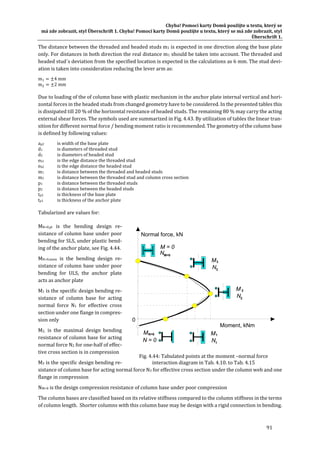

![Chyba! Pomocí karty Domů použijte u textu, který se má zde zobrazit, styl Überschrift 1. Chyba! Pomocí karty Domů
použijte u textu, který se má zde zobrazit, styl Überschrift 1.
93
Tab. 4.10: Recommended geometry of the column base with anchor plate, its design resistances, stiffness and limiting length for HE160B
HE160B
Column Base plate Anchor plate Threaded studs Headed studs Stirrups
awf = 6 mm S355 P25 ‐ 200 x 360 S355 P(tp1) ‐ 240 x (380 + 2m1) S355 Ø 24 mm S355 Ø 22 mm S355 Ø 8 mm
Foundation ea2 = 50 mm p2 = 100 mm ea1 = 60 mm p1 = 100 mm heff = 200 mm B500A
700 x 1200 x 850 C20/25 eb2 = 50 mm m2 = 50 mm eb1 = 70 mm 4 legs for stud
Varying Resistance / Stiffness / Limiting length
m1 tp1 MN=0,pl Sj,ini,pl MN=0,mem Lcb Lco M1 N1 Sj,ini Lcb Lco M2 N2 Sj,ini Lcb Lco M3 N3 Sj,ini Lcb Lco NM=0
[mm] [mm] [kNm] [kNm/rad] [kNm] [m] [m] [kNm] [kN] [kNm/rad] [m] [m] [kNm] [kN] [kNm/rad] [m] [m] [kNm] [kN] [kNm/rad] [m] [m] [kN]
0
10 53 15133 ‐ 2.8 8.6 95 700 13939 3.0 9.4 95 700 13939 3.0 9.4 95 700 13939 3.0 9.4 1804
12 54 15045 ‐ 2.8 8.7 100 742 13826 3.0 9.5 100 742 13826 3.0 9.5 100 742 13826 3.0 9.5 1887
15 55 14913 ‐ 2.8 8.8 108 806 13669 3.1 9.6 108 806 13669 3.1 9.6 108 806 13669 3.1 9.6 1926
50
10 31 6380 34 6.6 20.5 86 767 6301 6.6 20.8 86 767 6301 6.6 20.8 86 767 6301 6.6 20.8 1804
12 45 8683 48 4.8 15.1 98 756 8093 5.2 16.2 98 756 8093 5.2 16.2 98 756 8093 5.2 16.2 1887
15 65 10958 65 3.8 11.9 114 756 9917 4.2 13.2 114 756 9917 4.2 13.2 114 756 9917 4.2 13.2 1926
100
10 24 494 29 84.8 265.0 84 784 536 78.1 244.2 84 784 536 78.1 244.2 84 784 536 78.1 244.2 1804
12 35 950 39 44.1 137.7 94 785 930 45.0 140.7 94 785 930 45.0 140.7 94 785 930 45.0 140.7 1887
15 54 1953 58 21.4 67.0 112 775 1780 23.5 73.5 112 775 1780 23.5 73.5 112 775 1780 23.5 73.5 1926
HE160B
Column Base plate Anchor plate Threaded studs Headed studs Stirrups
awf = 6 mm S355 P30 ‐ 200 x 360 S355 P(tp1) ‐ 240 x (380 + 2m1) S355 Ø 24 mm S355 Ø 22 mm S355 Ø 8 mm
Foundation ea2 = 50 mm p2 = 100 mm ea1 = 60 mm p1 = 100 mm heff = 200 mm B500A
700 x 1200 x 850 C20/25 eb2 = 50 mm m2 = 50 mm eb1 = 70 mm 4 legs for stud
Varying Resistance / Stiffness / Limiting length
m1 tp1 MN=0,pl Sj,ini,pl MN=0,mem Lcb Lco M1 N1 Sj,ini Lcb Lco M2 N2 Sj,ini Lcb Lco M3 N3 Sj,ini Lcb Lco NM=0
[mm] [mm] [kNm] [kNm/rad] [kNm] [m] [m] [kNm] [kN] [kNm/rad] [m] [m] [kNm] [kN] [kNm/rad] [m] [m] [kNm] [kN] [kNm/rad] [m] [m] [kN]
0
10 55 16445 ‐ 2.5 8.0 105 762 15214 2.8 8.6 105 762 15214 2.8 8.6 105 762 15214 2.8 8.6 1926
12 56 16338 ‐ 2.6 8.0 110 805 15090 2.8 8.7 110 805 15090 2.8 8.7 110 805 15090 2.8 8.7 1926
15 57 16177 ‐ 2.6 8.1 119 871 14916 2.8 8.8 119 871 14916 2.8 8.8 119 871 14916 2.8 8.8 1926
50
10 33 6623 36 6.3 19.8 96 830 6616 6.3 19.8 96 830 6616 6.3 19.8 96 830 6616 6.3 19.8 1926
12 47 9103 49 4.6 14.4 108 820 8540 4.9 15.3 108 820 8540 4.9 15.3 108 820 8540 4.9 15.3 1926
15 67 11589 67 3.6 11.3 125 822 10519 4.0 12.4 125 822 10519 4.0 12.4 125 822 10519 4.0 12.4 1926
100
10 25 493 30 84.9 265.4 94 847 544 76.9 240.3 94 847 544 76.9 240.3 94 847 544 76.9 240.3 1926
12 36 952 41 44.0 137.4 105 850 943 44.4 138.7 105 850 943 44.4 138.7 105 850 943 44.4 138.7 1926
15 56 1968 60 21.3 66.5 123 841 1803 23.2 72.6 123 841 1803 23.2 72.6 123 841 1803 23.2 72.6 1926](https://image.slidesharecdn.com/boltdesign-manualiien-191004025827/85/Bolt-design-manual-ii-en-272-320.jpg)
![Infaso+‐Handbuch Teil I
94
Tab. 4.11: Recommended geometry of the column base with anchor plate, its design resistances, stiffness and limiting length for HE180B
HE180B
Column Base plate Anchor plate Threaded studs Headed studs Stirrups
awf = 6 mm S355 P25 ‐ 220 x 380 S355 P(tp1) ‐ 260 x (400 + 2m1) S355 M24 S355 Ø 22 mm S355 Ø 8 mm
Foundation ea2 = 50 mm p2 = 100 mm ea1 = 60 mm p1 = 100 mm heff = 200 mm B500A
800 x 1200 x 850 C25/30 eb2 = 60 mm m2 = 50 mm eb1 = 80 mm 4 legs for stud
Varying Resistance / Stiffness / Limiting length
m1 tp1 MN=0,pl Sj,ini,pl MN=0,mem Lcb Lco M1 N1 Sj,ini Lcb Lco M2 N2 Sj,ini Lcb Lco M3 N3 Sj,ini Lcb Lco NM=0
[mm] [mm] [kNm] [kNm/rad] [kNm] [m] [m] [kNm] [kN] [kNm/rad] [m] [m] [kNm] [kN] [kNm/rad] [m] [m] [kNm] [kN] [kNm/rad] [m] [m] [kN]
0
10 63 18604 ‐ 3.5 10.8 127 942 16566 3.9 12.1 127 989 16342 3.9 12.3 127 1036 16088 4.0 12.5 2316
12 63 18493 ‐ 3.5 10.9 134 1023 16299 3.9 12.3 134 1054 16160 4.0 12.4 134 1085 16009 4.0 12.6 2316
15 65 18325 ‐ 3.5 11.0 145 1148 15925 4.0 12.6 145 1151 15911 4.0 12.6 145 1154 15897 4.0 12.7 2316
50
10 36 8107 39 7.9 24.8 117 1022 7795 8.3 25.8 117 1069 7668 8.4 26.2 116 1116 7522 8.6 26.7 2316
12 52 10958 55 5.9 18.4 131 1046 9795 6.6 20.5 131 1077 9701 6.6 20.7 131 1107 9600 6.7 21.0 2316
15 74 13710 74 4.7 14.7 149 1114 11642 5.5 17.3 149 1117 11631 5.5 17.3 149 1120 11620 5.5 17.3 2316
100
10 27 659 33 97.6 305.1 114 1042 697 92.3 288.4 114 1089 685 94.0 293.8 113 1135 670 96.1 300.3 2316
12 40 1269 45 50.7 158.5 126 1080 1190 54.1 169.0 127 1110 1177 54.7 171.0 126 1141 1162 55.4 173.1 2316
15 62 2600 66 24.8 77.4 148 1123 2222 29.0 90.5 148 1126 2220 29.0 90.6 148 1129 2217 29.0 90.7 2316
HE180B
Column Base plate Anchor plate Threaded studs Headed studs Stirrups
awf = 6 mm S355 P30 ‐ 220 x 380 S355 P(tp1) ‐ 260 x (400 + 2m1) S355 M24 S355 Ø 22 mm S355 Ø 8 mm
Foundation ea2 = 50 mm p2 = 100 mm ea1 = 60 mm p1 = 100 mm heff = 200 mm B500A
800 x 1200 x 850 C25/30 eb2 = 60 mm m2 = 50 mm eb1 = 80 mm 4 legs for stud
Varying Resistance / Stiffness / Limiting length
m1 tp1 MN=0,pl Sj,ini,pl MN=0,mem Lcb Lco M1 N1 Sj,ini Lcb Lco M2 N2 Sj,ini Lcb Lco M3 N3 Sj,ini Lcb Lco NM=0
[mm] [mm] [kNm] [kNm/rad] [kNm] [m] [m] [kNm] [kN] [kNm/rad] [m] [m] [kNm] [kN] [kNm/rad] [m] [m] [kNm] [kN] [kNm/rad] [m] [m] [kN]
0
10 65 20062 ‐ 3.2 10.0 140 1093 17608 3.7 11.4 140 1096 17593 3.7 11.4 140 1099 17577 3.7 11.4 2316
12 66 19928 ‐ 3.2 10.1 147 1150 17448 3.7 11.5 147 1150 17448 3.7 11.5 147 1150 17448 3.7 11.5 2316
15 67 19728 ‐ 3.3 10.2 158 1231 17255 3.7 11.7 158 1231 17255 3.7 11.7 158 1231 17255 3.7 11.7 2316
50
10 37 8401 40 7.7 23.9 129 1173 7984 8.1 25.2 129 1177 7976 8.1 25.2 129 1180 7967 8.1 25.2 2316
12 54 11456 56 5.6 17.6 144 1174 10173 6.3 19.8 144 1174 10173 6.3 19.8 144 1174 10173 6.3 19.8 2316
15 77 14458 77 4.5 13.9 163 1197 12328 5.2 16.3 163 1197 12328 5.2 16.3 163 1197 12328 5.2 16.3 2316
100
10 28 659 34 97.7 305.3 126 1193 691 93.2 291.3 126 1196 690 93.3 291.6 126 1200 689 93.4 292.0 2316
12 41 1272 46 50.6 158.1 139 1208 1188 54.2 169.2 139 1208 1188 54.2 169.2 139 1208 1188 54.2 169.2 2316
15 64 2621 68 24.6 76.7 161 1208 2254 28.6 89.2 161 1208 2254 28.6 89.2 161 1208 2254 28.6 89.2 2316](https://image.slidesharecdn.com/boltdesign-manualiien-191004025827/85/Bolt-design-manual-ii-en-273-320.jpg)
![Chyba! Pomocí karty Domů použijte u textu, který se má zde zobrazit, styl Überschrift 1. Chyba! Pomocí karty Domů
použijte u textu, který se má zde zobrazit, styl Überschrift 1.
95
Tab. 4.12: Recommended geometry of the column base with anchor plate, its design resistances, stiffness and limiting length for HE200B
HE200B
Column Base plate Anchor plate Threaded studs Headed studs Stirrups
awf = 6 mm S355 P25 ‐ 240 x 400 S355 P(tp1) ‐ 280 x (420 + 2m1) S355 M24 S355 Ø 22 mm S355 Ø 8 mm
Foundation ea2 = 50 mm p2 = 120 mm ea1 = 60 mm p1 = 120 mm heff = 200 mm B500A
800 x 1300 x 900 C25/30 eb2 = 60 mm m2 = 50 mm eb1 = 80 mm 4 legs for stud
Varying Resistance / Stiffness / Limiting length
m1 tp1 MN=0,pl Sj,ini,pl MN=0,mem Lcb Lco M1 N1 Sj,ini Lcb Lco M2 N2 Sj,ini Lcb Lco M3 N3 Sj,ini Lcb Lco NM=0
[mm] [mm] [kNm] [kNm/rad] [kNm] [m] [m] [kNm] [kN] [kNm/rad] [m] [m] [kNm] [kN] [kNm/rad] [m] [m] [kNm] [kN] [kNm/rad] [m] [m] [kN]
0
10 69 22107 ‐ 2.9 9.1 152 1041 19735 3.3 10.2 152 1131 19257 3.3 10.4 148 1220 18664 3.4 10.8 2725
12 70 21967 ‐ 2.9 9.2 160 1127 19423 3.3 10.4 160 1203 19043 3.4 10.6 157 1279 18588 3.5 10.8 2772
15 71 21758 ‐ 3.0 9.2 172 1260 18985 3.4 10.6 172 1311 18748 3.4 10.7 171 1363 18483 3.5 10.9 2772
50
10 38 9400 42 6.8 21.4 139 1131 9302 6.9 21.6 139 1219 9036 7.1 22.3 135 1308 8696 7.4 23.1 2725
12 55 12865 58 5.0 15.6 155 1160 11676 5.5 17.2 155 1235 11421 5.6 17.6 153 1310 11117 5.8 18.1 2772
15 80 16297 80 3.9 12.3 176 1232 13907 4.6 14.5 176 1284 13721 4.7 14.7 175 1335 13514 4.8 14.9 2772
100
10 29 756 35 85.1 266.0 135 1152 837 76.9 240.3 136 1240 810 79.4 248.2 132 1328 776 82.9 259.1 2725
12 42 1472 47 43.7 136.6 150 1195 1424 45.2 141.2 150 1270 1389 46.3 144.8 148 1344 1346 47.8 149.4 2772
15 66 3058 70 21.0 65.8 174 1248 2651 24.3 75.9 174 1298 2612 24.6 77.0 173 1349 2567 25.1 78.3 2772
HE200B
Column Base plate Anchor plate Threaded studs Headed studs Stirrups
awf = 6 mm S355 P30 ‐ 240 x 400 S355 P(tp1) ‐ 280 x (420 + 2m1) S355 M24 S355 Ø 22 mm S355 Ø 8 mm
Foundation ea2 = 50 mm p2 = 120 mm ea1 = 60 mm p1 = 120 mm heff = 200 mm B500A
800 x 1300 x 900 C25/30 eb2 = 60 mm m2 = 50 mm eb1 = 80 mm 4 legs for stud
Varying Resistance / Stiffness / Limiting length
m1 tp1 MN=0,pl Sj,ini,pl MN=0,mem Lcb Lco M1 N1 Sj,ini Lcb Lco M2 N2 Sj,ini Lcb Lco M3 N3 Sj,ini Lcb Lco NM=0
[mm] [mm] [kNm] [kNm/rad] [kNm] [m] [m] [kNm] [kN] [kNm/rad] [m] [m] [kNm] [kN] [kNm/rad] [m] [m] [kNm] [kN] [kNm/rad] [m] [m] [kN]
0
10 71 23682 ‐ 2.7 8.5 167 1205 20840 3.1 9.7 167 1256 20579 3.1 9.8 166 1307 20286 3.2 9.9 2772
12 72 23518 ‐ 2.7 8.6 175 1293 20524 3.1 9.8 175 1326 20367 3.2 9.9 174 1359 20198 3.2 10.0 2772
15 74 23274 ‐ 2.8 8.6 187 1430 20077 3.2 10.0 187 1431 20071 3.2 10.0 187 1432 20066 3.2 10.0 2772
50
10 39 9709 43 6.6 20.7 154 1294 9508 6.8 21.2 154 1345 9366 6.9 21.5 153 1396 9206 7.0 21.8 2772
12 57 13398 60 4.8 15.0 170 1326 12005 5.4 16.8 170 1358 11901 5.4 16.9 170 1391 11790 5.5 17.1 2772
15 82 17112 82 3.8 11.8 192 1402 14392 4.5 14.0 192 1403 14388 4.5 14.0 192 1404 14384 4.5 14.0 2772
100
10 30 756 35 85.2 266.2 151 1315 830 77.6 242.4 151 1366 816 78.9 246.5 150 1416 800 80.4 251.3 2772
12 43 1476 48 43.6 136.3 165 1361 1412 45.6 142.4 165 1393 1398 46.0 143.8 165 1425 1383 46.5 145.4 2772
15 67 3081 72 20.9 65.3 189 1418 2633 24.4 76.4 189 1419 2633 24.4 76.4 189 1420 2632 24.5 76.4 2772](https://image.slidesharecdn.com/boltdesign-manualiien-191004025827/85/Bolt-design-manual-ii-en-274-320.jpg)
![Infaso+‐Handbuch Teil I
96
Tab. 4.13: Recommended geometry of the column base with anchor plate, its design resistances, stiffness and limiting length for HE220B
HE220B
Column Base plate Anchor plate Threaded studs Headed studs Stirrups
awf = 6 mm S355 P25 ‐ 260 x 420 S355 P(tp1) ‐ 300 x (440 + 2m1) S355 M24 S355 Ø 22 mm S355 Ø 8 mm
Foundation ea2 = 50 mm p2 = 120 mm ea1 = 60 mm p1 = 120 mm heff = 200 mm B500A
900 x 1400 x 1000 C25/30 eb2 = 70 mm m2 = 50 mm eb1 = 90 mm 4 legs for stud
Varying Resistance / Stiffness / Limiting length
m1 tp1 MN=0,pl Sj,ini,pl MN=0,mem Lcb Lco M1 N1 Sj,ini Lcb Lco M2 N2 Sj,ini Lcb Lco M3 N3 Sj,ini Lcb Lco NM=0
[mm] [mm] [kNm] [kNm/rad] [kNm] [m] [m] [kNm] [kN] [kNm/rad] [m] [m] [kNm] [kN] [kNm/rad] [m] [m] [kNm] [kN] [kNm/rad] [m] [m] [kN]
0
10 74 25718 ‐ 2.5 7.8 177 1149 23107 2.8 8.7 177 1411 21614 3.0 9.3 162 1672 19614 3.3 10.3 3232
12 75 25547 ‐ 2.5 7.9 186 1240 22751 2.8 8.8 186 1470 21509 3.0 9.4 175 1700 19909 3.2 10.1 3232
15 76 25291 ‐ 2.5 8.0 201 1380 22250 2.9 9.0 201 1560 21351 3.0 9.4 194 1740 20258 3.2 9.9 3232
50
10 41 10735 44 6.0 18.7 161 1221 10963 5.9 18.3 161 1468 10175 6.3 19.8 148 1714 9108 7.1 22.1 3220
12 59 14863 62 4.3 13.5 179 1256 13750 4.7 14.6 179 1470 12962 5.0 15.5 169 1685 11958 5.4 16.8 3232
15 85 19056 85 3.4 10.6 203 1331 16407 3.9 12.3 203 1498 15742 4.1 12.8 197 1665 14953 4.3 13.5 3232
100
10 30 855 36 75.3 235.3 157 1243 992 64.9 202.8 158 1489 913 70.5 220.3 145 1734 807 79.7 249.1 3220
12 44 1683 49 38.3 119.5 173 1291 1685 38.2 119.4 173 1506 1575 40.9 127.7 164 1719 1437 44.8 140.0 3232
15 69 3539 74 18.2 56.8 199 1352 3128 20.6 64.3 200 1517 2987 21.5 67.3 194 1681 2821 22.8 71.3 3232
HE220B
Column Base plate Anchor plate Threaded studs Headed studs Stirrups
awf = 6 mm S355 P30 ‐ 260 x 420 S355 P(tp1) ‐ 300 x (440 + 2m1) S355 M24 S355 Ø 22 mm S355 Ø 8 mm
Foundation ea2 = 50 mm p2 = 120 mm ea1 = 60 mm p1 = 120 mm heff = 200 mm B500A
900 x 1400 x 1000 C25/30 eb2 = 70 mm m2 = 50 mm eb1 = 90 mm 4 legs for stud
Varying Resistance / Stiffness / Limiting length
m1 tp1 MN=0,pl Sj,ini,pl MN=0,mem Lcb Lco M1 N1 Sj,ini Lcb Lco M2 N2 Sj,ini Lcb Lco M3 N3 Sj,ini Lcb Lco NM=0
[mm] [mm] [kNm] [kNm/rad] [kNm] [m] [m] [kNm] [kN] [kNm/rad] [m] [m] [kNm] [kN] [kNm/rad] [m] [m] [kNm] [kN] [kNm/rad] [m] [m] [kN]
0
10 76 27392 ‐ 2.3 7.3 195 1325 24272 2.7 8.3 195 1498 23316 2.8 8.6 188 1672 22155 2.9 9.1 3232
12 77 27194 ‐ 2.4 7.4 204 1418 23913 2.7 8.4 204 1559 23178 2.8 8.7 200 1700 22319 2.9 9.0 3232
15 78 26901 ‐ 2.4 7.5 219 1562 23405 2.7 8.6 219 1651 22973 2.8 8.8 217 1740 22498 2.9 8.9 3232
50
10 42 11057 45 5.8 18.2 179 1395 11184 5.8 18.0 179 1555 10702 6.0 18.8 173 1716 10113 6.4 19.9 3232
12 60 15426 63 4.2 13.0 197 1432 14102 4.6 14.3 197 1559 13658 4.7 14.7 193 1687 13145 4.9 15.3 3232
15 88 19931 88 3.2 10.1 221 1511 16924 3.8 11.9 221 1588 16630 3.9 12.1 220 1665 16312 3.9 12.3 3232
100
10 31 854 37 75.4 235.5 175 1417 984 65.4 204.4 175 1577 937 68.7 214.6 170 1736 880 73.1 228.5 3232
12 45 1686 51 38.2 119.3 191 1468 1672 38.5 120.3 191 1595 1612 39.9 124.8 188 1721 1543 41.7 130.3 3232
15 71 3563 75 18.1 56.5 218 1532 3108 20.7 64.7 218 1608 3048 21.1 66.0 217 1684 2983 21.6 67.4 3232](https://image.slidesharecdn.com/boltdesign-manualiien-191004025827/85/Bolt-design-manual-ii-en-275-320.jpg)
![Chyba! Pomocí karty Domů použijte u textu, který se má zde zobrazit, styl Überschrift 1. Chyba! Pomocí karty Domů
použijte u textu, který se má zde zobrazit, styl Überschrift 1.
97
Tab. 4.14: Recommended geometry of the column base with anchor plate, its design resistances, stiffness and limiting length for HE240B
HE240B
Column Base plate Anchor plate Threaded studs Headed studs Stirrups
awf = 6 mm S355 P25 ‐ 280 x 440 S355 P(tp1) ‐ 320 x (460 + 2m1) S355 M24 S355 Ø 22 mm S355 Ø 8 mm
Foundation ea2 = 50 mm p2 = 140 mm ea1 = 60 mm p1 = 140 mm heff = 200 mm B500A
900 x 1400 x 1000 C25/30 eb2 = 70 mm m2 = 50 mm eb1 = 90 mm 4 legs for stud
Varying Resistance / Stiffness / Limiting length
m1 tp1 MN=0,pl Sj,ini,pl MN=0,mem Lcb Lco M1 N1 Sj,ini Lcb Lco M2 N2 Sj,ini Lcb Lco M3 N3 Sj,ini Lcb Lco NM=0
[mm] [mm] [kNm] [kNm/rad] [kNm] [m] [m] [kNm] [kN] [kNm/rad] [m] [m] [kNm] [kN] [kNm/rad] [m] [m] [kNm] [kN] [kNm/rad] [m] [m] [kN]
0
10 81 29714 ‐ 2.2 6.8 206 1251 26832 2.4 7.5 206 1426 25704 2.5 7.8 193 1601 24068 2.7 8.4 3328
12 82 29509 ‐ 2.2 6.8 216 1347 26425 2.4 7.6 216 1513 25420 2.5 7.9 205 1679 24010 2.7 8.4 3502
15 83 29205 ‐ 2.2 6.9 233 1495 25853 2.5 7.8 233 1643 25031 2.6 8.0 225 1791 23934 2.7 8.4 3763
50
10 43 12106 47 5.3 16.6 183 1292 12783 5.0 15.7 183 1448 12204 5.3 16.5 172 1605 11359 5.7 17.7 3176
12 62 16942 65 3.8 11.9 202 1329 16025 4.0 12.6 202 1476 15408 4.2 13.1 193 1621 14560 4.4 13.8 3341
15 91 21975 91 2.9 9.2 229 1407 19151 3.4 10.5 229 1535 18567 3.5 10.8 222 1663 17821 3.6 11.3 3588
100
10 32 955 38 67.4 210.7 179 1314 1162 55.4 173.1 179 1470 1104 58.3 182.2 168 1626 1019 63.1 197.3 3176
12 46 1898 52 33.9 106.0 196 1366 1971 32.7 102.0 196 1512 1886 34.1 106.7 187 1657 1768 36.4 113.8 3341
15 73 4040 78 15.9 49.8 224 1433 3653 17.6 55.1 225 1559 3529 18.2 57.0 219 1685 3372 19.1 59.6 3588
HE240B
Column Base plate Anchor plate Threaded studs Headed studs Stirrups
awf = 6 mm S355 P30 ‐ 280 x 440 S355 P(tp1) ‐ 320 x (460 + 2m1) S355 M24 S355 Ø 22 mm S355 Ø 8 mm
Foundation ea2 = 50 mm p2 = 140 mm ea1 = 60 mm p1 = 140 mm heff = 200 mm B500A
900 x 1400 x 1000 C25/30 eb2 = 70 mm m2 = 50 mm eb1 = 90 mm 4 legs for stud
Varying Resistance / Stiffness / Limiting length
m1 tp1 MN=0,pl Sj,ini,pl MN=0,mem Lcb Lco M1 N1 Sj,ini Lcb Lco M2 N2 Sj,ini Lcb Lco M3 N3 Sj,ini Lcb Lco NM=0
[mm] [mm] [kNm] [kNm/rad] [kNm] [m] [m] [kNm] [kN] [kNm/rad] [m] [m] [kNm] [kN] [kNm/rad] [m] [m] [kNm] [kN] [kNm/rad] [m] [m] [kN]
0
10 83 31486 ‐ 2.0 6.4 227 1439 28047 2.3 7.2 227 1587 27147 2.4 7.4 218 1735 25948 2.5 7.8 3651
12 84 31253 ‐ 2.1 6.4 238 1538 27640 2.3 7.3 238 1672 26870 2.4 7.5 231 1806 25880 2.5 7.8 3763
15 86 30907 ‐ 2.1 6.5 254 1690 27062 2.4 7.4 254 1799 26484 2.4 7.6 251 1908 25779 2.5 7.8 3763
50
10 44 12436 48 5.2 16.2 203 1473 13017 4.9 15.5 203 1601 12582 5.1 16.0 197 1728 12007 5.4 16.8 3481
12 64 17530 67 3.7 11.5 223 1514 16396 3.9 12.3 223 1626 15954 4.0 12.6 218 1738 15401 4.2 13.1 3641
15 93 22905 93 2.8 8.8 250 1594 19694 3.3 10.2 250 1681 19320 3.3 10.4 247 1769 18885 3.4 10.7 3763
100
10 33 954 39 67.5 210.9 199 1496 1153 55.8 174.4 199 1623 1111 57.9 181.0 193 1750 1055 61.0 190.6 3481
12 47 1901 53 33.9 105.8 216 1550 1957 32.9 102.8 217 1662 1897 33.9 106.0 212 1774 1823 35.3 110.3 3641
15 74 4064 79 15.8 49.5 245 1621 3631 17.7 55.4 246 1706 3554 18.1 56.6 243 1792 3465 18.6 58.0 3763](https://image.slidesharecdn.com/boltdesign-manualiien-191004025827/85/Bolt-design-manual-ii-en-276-320.jpg)
![Infaso+‐Handbuch Teil I
98
Tab. 4.15: Recommended geometry of the column base with anchor plate, its design resistances, stiffness and limiting length for HE260B
HE260B
Column Base plate Anchor plate Threaded studs Headed studs Stirrups
awf = 6 mm S355 P25 ‐ 300 x 460 S355 P(tp1) ‐ 340 x (480 + 2m1) S355 M24 S355 Ø 22 mm S355 Ø 8 mm
Foundation ea2 = 50 mm p2 = 140 mm ea1 = 60 mm p1 = 140 mm heff = 200 mm B500A
100 x 1500 x 1050 C25/30 eb2 = 80 mm m2 = 50 mm eb1 = 100 mm 4 legs for stud
Varying Resistance / Stiffness / Limiting length
m1 tp1 MN=0,pl Sj,ini,pl MN=0,mem Lcb Lco M1 N1 Sj,ini Lcb Lco M2 N2 Sj,ini Lcb Lco M3 N3 Sj,ini Lcb Lco NM=0
[mm] [mm] [kNm] [kNm/rad] [kNm] [m] [m] [kNm] [kN] [kNm/rad] [m] [m] [kNm] [kN] [kNm/rad] [m] [m] [kNm] [kN] [kNm/rad] [m] [m] [kN]
0
10 86 33765 ‐ 1.9 6.0 235 1355 30797 2.1 6.5 235 1576 29258 2.2 6.9 215 1796 26868 2.4 7.5 3627
12 87 33523 ‐ 1.9 6.0 247 1457 30340 2.1 6.6 247 1670 28938 2.2 7.0 229 1883 26826 2.4 7.5 3816
15 88 33164 ‐ 1.9 6.1 266 1613 29698 2.2 6.8 266 1811 28498 2.3 7.1 251 2010 26774 2.4 7.5 4099
50
10 45 13518 49 4.8 14.9 204 1346 14783 4.4 13.6 204 1531 14019 4.6 14.3 189 1716 12847 5.0 15.7 3339
12 66 19111 69 3.4 10.5 225 1386 18528 3.5 10.9 225 1563 17694 3.6 11.4 212 1738 16489 3.9 12.2 3511
15 97 25071 97 2.6 8.0 255 1465 22170 2.9 9.1 255 1625 21346 3.0 9.4 244 1786 20242 3.2 9.9 3769
100
10 34 1057 40 60.9 190.4 200 1369 1350 47.7 149.0 200 1554 1273 50.5 157.9 185 1738 1156 55.7 174.0 3339
12 48 2120 55 30.4 94.9 218 1424 2287 28.1 87.9 219 1600 2172 29.6 92.6 206 1774 2005 32.1 100.3 3511
15 76 4563 81 14.1 44.1 249 1495 4232 15.2 47.5 250 1654 4059 15.9 49.6 240 1811 3827 16.8 52.6 3769
HE260B
Column Base plate Anchor plate Threaded studs Headed studs Stirrups
awf = 6 mm S355 P30 ‐ 300 x 460 S355 P(tp1) ‐ 340 x (480 + 2m1) S355 M24 S355 Ø 22 mm S355 Ø 8 mm
Foundation ea2 = 50 mm p2 = 140 mm ea1 = 60 mm p1 = 140 mm heff = 200 mm B500A
100 x 1500 x 1050 C25/30 eb2 = 80 mm m2 = 50 mm eb1 = 100 mm 4 legs for stud
Varying Resistance / Stiffness / Limiting length
m1 tp1 MN=0,pl Sj,ini,pl MN=0,mem Lcb Lco M1 N1 Sj,ini Lcb Lco M2 N2 Sj,ini Lcb Lco M3 N3 Sj,ini Lcb Lco NM=0
[mm] [mm] [kNm] [kNm/rad] [kNm] [m] [m] [kNm] [kN] [kNm/rad] [m] [m] [kNm] [kN] [kNm/rad] [m] [m] [kNm] [kN] [kNm/rad] [m] [m] [kN]
0
10 88 35615 ‐ 1.8 5.6 259 1556 32062 2.0 6.3 259 1755 30753 2.1 6.5 245 1954 28875 2.2 7.0 3987
12 89 35342 ‐ 1.8 5.7 272 1660 31606 2.0 6.4 272 1847 30442 2.1 6.6 260 2035 28824 2.2 7.0 4171
15 90 34940 ‐ 1.8 5.8 291 1820 30960 2.1 6.5 291 1986 30008 2.1 6.7 282 2152 28750 2.2 7.0 4203
50
10 46 13855 50 4.6 14.5 227 1534 15027 4.3 13.4 227 1694 14420 4.5 13.9 217 1854 13571 4.7 14.8 3665
12 67 19720 71 3.3 10.2 248 1577 18914 3.4 10.6 248 1724 18271 3.5 11.0 240 1870 17420 3.7 11.5 3832
15 99 26050 99 2.5 7.7 278 1659 22735 2.8 8.8 278 1782 22141 2.9 9.1 273 1906 21409 3.0 9.4 4083
100
10 34 1056 41 61.0 190.5 223 1557 1340 48.0 150.0 223 1717 1281 50.2 157.0 213 1876 1198 53.7 167.8 3665
12 50 2123 56 30.3 94.8 242 1615 2271 28.3 88.6 242 1761 2185 29.5 92.0 234 1906 2071 31.1 97.1 3832
15 78 4588 83 14.0 43.8 273 1689 4207 15.3 47.8 273 1811 4086 15.8 49.2 268 1933 3936 16.4 51.1 4083](https://image.slidesharecdn.com/boltdesign-manualiien-191004025827/85/Bolt-design-manual-ii-en-277-320.jpg)
![Chyba! Pomocí karty Domů použijte u textu, který se
má zde zobrazit, styl Überschrift 1. Chyba! Pomocí karty Domů použijte u textu, který se má zde zobrazit, styl
Überschrift 1.
99
4.5 Parameter study on composite joints
General
Composite joint behaviour depends on the characteristics of several active components. The hogging mo‐
ment capacity can be calculated with the hypothesis of failure of the weakest of them, while the total dis‐
placement (and relative rotation) can be found considering the contribution of all of them. The following
basic components are identified in Design Manual I "Design of steel‐to‐concrete joints" [13]: i) longitudinal
steel reinforcement in the slab; ii) slip of the composite beam; ii) beam web and flange; iv) steel contact
plate; v) components activated in the anchor plate connection; vi) the joint link. Among them, the longitu‐
dinal steel reinforcement transfers the tension force; the others contribute to the transmission of the com‐
pression force. Failure that depends on the steel reinforcement behaviour is ductile, while failure of con‐
crete components is brittle and should be avoided. The aim of this investigation is to evaluate the failure
mechanism of the joint in order to ensure a ductile failure. For this reason, a parametric study followed by
sensitivity analysis is carried out, taking into account the variation of some parameters that determine the
behaviour of basic components.
Parameters Studied and methodology followed
The attention is mainly focused on the behaviour of steel reinforcement and the joint link. The force in the
reinforcement is a function of the steel grade and of bars layout. The first aspect concerns the yield strength
(fsyk), the coefficient between the ultimate and yield strength (k) and ductility (εs,u).The second one is char‐
acterized by number and diameter of bars and number of layers. In the analysis three values of fsyk, four
values of k, three εs,u values and four reinforcement layouts are considered. The possibility of development
of the strut&tie mechanism in the concrete panel depends on the angle θ. This geometrical quantity is cal‐
culated through the ratio between the sum of beam height and slab thickness on the thickness of the wall.
In the analysis, six beam profiles, four wall thickness twall and three slab thickness sslab are considered. Wall
concrete properties, i.e. the characteristic compressive cylinder (fck,cyl) and cubic (fck,cube) strength, and se‐
cant modulus of elasticity (Ecm), affect as well the joint link behaviour. In the analysis five concrete grades
for wall are considered. The sensitivity analysis compared by 51840 combinations. Tab. 4.16 summarizes
the parameters considered for the parameter study.
Tab. 4.16: Parameters considered for parameter study
Element Parameter
Reinforcement
Yield strength
fsyk[MPa] 400 500 600
Coefficient fu/fsyk
k [‐] 1.05 1.15 1.25 1.35
Ductility
εs,u [‰] 25 50 75
Bar layout
N layers [‐]
N bars [‐]
Diameter bars [mm]
Case A
1
6
12
Case B
1
6
14
Case C
1
6
16
Case D
2
6
16
Slab
Thickness
tslab [mm] 120 160 200
Wall
Thickness
twall [mm] 160 200 240 300
Concrete grade
fck,cyl[MPa]
fck,cube[MPa]
Ecm[MPa]
20
25
30
30
37
33
40
50
35
50
60
37
60
75
39
Beam
Profile
IPE 240 IPE 270 IPE 300 IPE 330 IPE 360 IPE 400](https://image.slidesharecdn.com/boltdesign-manualiien-191004025827/85/Bolt-design-manual-ii-en-278-320.jpg)
![Infaso+‐Handbook II
100
Failure Mechanism
Considering the simultaneous variation of all parameters, the most common failure type is the joint link
(34149 cases of 51840, 65.87%); only in 14493 cases (27.96) a slab reinforcement failure occurs; in few
cases (3198, 6.17%) the failure depends on the behaviour of beam. Fig. 4.45 summarizes found failure types
in the sensitivity analysis.
Fig. 4.45: Failure type
Valorization of slab reinforcement properties
The role of slab reinforcement layout is studied, taking into account four bars configurations, according to
Tab. 4.16. Fig. 4.46 illustrates the influence. Increasing the reinforcement area, incidence of joint link failure
grows significantly, while reinforcement failure decreases. The trend is reversed considering the reinforce‐
ments on two layers (Case D). Beam failure is almost absent for low values of steel area, but it assumes a
quite relevant rate in Case D.
Fig. 4.46: Influence of rebar layout
As expected, one of the most influential parameter is the steel grade (see Fig. 4.47).Here, increasing the yield
strength, the percentage of joint link failure switches from 49.65 to 75.67, while cases with ductile failure
decrease. Variation of ductility of the bar does not lead to changes in failure type distribution.
6.17
65.87
27.96
Beam Web and Flange
Joint Link
Reinforcement
0.00 0.65
4.81
19.21
62.43
73.56
80.49
47.01
37.57
25.79
14.70
33.77
0.00
20.00
40.00
60.00
80.00
100.00
Case A Case B Case C Case D
FailureMechanism[%]
Bar Layout [-]
Beam Joint Link Reinforcement](https://image.slidesharecdn.com/boltdesign-manualiien-191004025827/85/Bolt-design-manual-ii-en-279-320.jpg)
![Chyba! Pomocí karty Domů použijte u textu, který se
má zde zobrazit, styl Überschrift 1. Chyba! Pomocí karty Domů použijte u textu, který se má zde zobrazit, styl
Überschrift 1.
101
Fig. 4.47: Influence of yield strength of slab reinforcement
The coefficient k influence is highlighted in Fig. 4.48. Increasing k, joint link failures number rises, while
cases of reinforcement failure are approximately halved.
Fig. 4.48: Influence of coefficient k
The interaction between the yield and ultimate strength is evaluated in Fig. 4.49. A change of the main fail‐
ure type is visible for yield strength equal to 400MPa. While the joint link is crucial for high values of k (61%
of failures), the longitudinal reinforcement becomes the most important component for a lower value of k
(57% of failures). The number of cases with joint link failure grows significantly (+20%) with increasing k
for a steel with a low value of yield strength (fsyk= 400 MPa). The same trend is visible for a steel with greater
yield strength (fsyk =600 MPa), but the increase is lower (10%).
1.09
5.81
9.12
49.65
65.25
75.67
49.26
28.94
15.21
0.00
20.00
40.00
60.00
80.00
100.00
400 500 600
FailureMechanism[%]
fsyk [MPa]
Beam Joint Link Reinforcement
1.09
5.81
9.12
49.65
65.25
75.67
49.26
28.94
15.21
0.00
20.00
40.00
60.00
80.00
100.00
400 500 600
FailureMechanism[%]
fsyk [MPa]
Beam Joint Link Reinforcement](https://image.slidesharecdn.com/boltdesign-manualiien-191004025827/85/Bolt-design-manual-ii-en-280-320.jpg)
![Infaso+‐Handbook II
102
Fig. 4.49: Interaction between yield and ultimate strength
Variation of angle θ
In order to assess the role of the angle theta, the influence of the individual parameters (twall, tslab and hbeam)
is studied. In addition, the total height (slab + beam) has been considered. The main parameter that affects
the development of the failure mechanism is the wall thickness. For a thickness of 160 mm in 93.45% of
cases the failure occurs in the concrete panel. The number of cases of brittle failure drops to 76.04 for a
thickness of 200 mm (Fig. 4.50). The ductile failure becomes the main type of failure only for a thickness of
300 mm.
7.08 9.51
10.76 11.81
71.25
76.04
79.72
82.22
21.67
14.44
9.51
5.973.26 7.08 7.08
9.51
59.51
65.63
70.63
75.07
27.29 27.29
22.29
15.42
0.00 0.00 3.26 4.65
42.85 49.79
56.32
61.46
57.15
50.21
40.42
33.89
0
20
40
60
80
100
1.05 1.15 1.25 1.35
FailureMechanism[%]
k [-]
Beam fsyk 600 MPa Joint Link fsyk 600 MPa Reinforcement fsyk 600 MPa
Beam fsyk 500 MPa Joint Link fsyk 500 MPa Reinforcement fsyk 500 MPa
Beam fsyk 400 MPa Joint Link fsyk 400 MPa Reinforcement fsyk 400 MPa](https://image.slidesharecdn.com/boltdesign-manualiien-191004025827/85/Bolt-design-manual-ii-en-281-320.jpg)
![Chyba! Pomocí karty Domů použijte u textu, který se
má zde zobrazit, styl Überschrift 1. Chyba! Pomocí karty Domů použijte u textu, který se má zde zobrazit, styl
Überschrift 1.
103
Fig. 4.50: Influence of twall
The influence of the slab thickness is shown in Fig. 4.51. For the three values considered (120, 160, 200),
structural failure happens in the concrete panel in most of the cases (variation between 55.09% and
67.34%). The percentage of beam failure does not vary appreciably. The increase in the height of the beam
determines a clear trend, as seen in Fig. 4.52. For a height of 240 mm, in about 50% of cases the failure
happens for the concrete panel. Here, the number of cases with beam failure is not negligible (22%). With
the increase of the height, the possibility of a failure in the beam decreases significantly, increasing sharply
the percentage of the failure in the concrete panel. The consideration of the total height (slab + beam) leads
to a less clear trend for low values (Fig. 4.53).
Fig. 4.51: Influence of tslab
2.34
5.09
7.55 9.70
93.45
76.04
56.94
37.06
4.21
18.87
35.51
53.24
0.00
20.00
40.00
60.00
80.00
100.00
160 200 240 300
FailureMechanism[%]
twall [mm]
Beam Joint Link Reinforcement
5.32 4.68 3.98
55.09
61.74
67.34
39.58
33.59
28.68
0.00
20.00
40.00
60.00
80.00
100.00
120 160 200
FailureMechanism[%]
tslab [mm]
Beam Joint Link Reinforcement](https://image.slidesharecdn.com/boltdesign-manualiien-191004025827/85/Bolt-design-manual-ii-en-282-320.jpg)
![Infaso+‐Handbook II
104
Fig. 4.52: Influence of hbeam
Fig. 4.53: Influence of total height
Initial beam failure peaks (26.46%, 22.7% and 19.38%) are due to the presence of IPE240. However, joint
link represents always the main failure type and the possibility of brittle crisis doubles, moving from a
height of 360 mm (41.67%) to 600 mm (82.08).
Variation of wall concrete grade
The concrete grade is an important parameter. Fig. 4.54 shows the variation of number of case for each
mechanism failure type. For concrete grade C20/25, joint link behaviour represents the limit condition in
almost all of the cases (97.25%). The variation is evident. This percentage drops to 36.86 % for concrete
C60/75. Brittle failure is the most probable event for fck,wall is smaller than 40MPa.
22.85 9.90
3.75 0.52 0 0
49.34
58.85
65.14
69.76
78.29 78.3
27.81
31.25 31.11 29.72
21.71 21.7
0.00
20.00
40.00
60.00
80.00
100.00
240 270 300 330 360 400
FailureMechanism[%]
hbeam [mm]
Beam Joint Link Reinforcement
26.46 11.56
22.71 4.17
10.00
19.38
0.63
3.96
8.13
0.00 0.52
3.13
0.00 0.42 0.00 0.00
41.67
51.98
49.69
58.96 58.85 56.67
64.17 65.63 65.73
68.75 70.10 70.83
73.96 75.00
78.85
82.08
31.88
36.46
27.60
36.88
31.15
23.96
35.21
30.42
26.15
31.25 29.38
26.04 26.04 24.58
21.15
17.92
0.00
20.00
40.00
60.00
80.00
100.00
360 390 400 420 430 440 450 460 470 480 490 500 520 530 560 600
FailureMechanism[%]
hbeam [mm]
Beam Joint Link Reinforcement](https://image.slidesharecdn.com/boltdesign-manualiien-191004025827/85/Bolt-design-manual-ii-en-283-320.jpg)
![Chyba! Pomocí karty Domů použijte u textu, který se
má zde zobrazit, styl Überschrift 1. Chyba! Pomocí karty Domů použijte u textu, který se má zde zobrazit, styl
Überschrift 1.
105
Fig. 4.54: Influence of wall concrete grade
Interaction between wall thickness and concrete grade
The interaction between geometrical properties and material of the wall is studied. For a thickness of 160
mm, joint link determines the failure for all types of concrete considered (Fig. 4.54).
Fig. 4.55: Influence of wall concrete grade for twall = 160 mm
The percentage drops from 100% (C20/25) to 81.94% (C60/75). The decrease in the percentage of brittle
failure is more pronounced for a thickness of 200 mm (Fig. 4.56). In this case for C60/75, ductile failure is
more probable than a brittle failure (44.68%).
1.16
3.79
6.94
9.00 9.92
97.25 83.97
63.74
47.80
36.86
1.59
12.24
29.31 43.20
53.22
0.00
20.00
40.00
60.00
80.00
100.00
20 29.6 40 50 60
FailureMechanism[%]
fckcylWall [MPa]
Beam Web and Flange Joint Link Reinforcement
0.00 0.00 2.31
4.28
5.09
100.00 99.88
96.06
89.35
81.94
0.00
2.78 1.62
6.37
12.96
0.00
20.00
40.00
60.00
80.00
100.00
20.00 29.6 40 50 60
FailureMechanism[%]
fckcylWall [MPa]
twall = 160 mm
Beam Joint Link Reinforcement](https://image.slidesharecdn.com/boltdesign-manualiien-191004025827/85/Bolt-design-manual-ii-en-284-320.jpg)
![Infaso+‐Handbook II
106
Fig. 4.56: Influence of wall concrete grade for twall = 200 mm
With a wall thickness of 240mm (Fig. 4.57), the increase of reinforcement failure is evident. It represents
0.96% of the cases for fck,Wall equal to 20 MPa and becomes 70.37 % when fck,Wall is 60 MPa. Reduction of joint
link failures is noteworthy. From 97.92% (C20/25) to 17.59% (C60/75). Considering a wall thickness of
300 mm (Fig. 4.58), the inversion of most probable failure type (from brittle to ductile) occurs for concrete
grade C40/50. A strong change in the trend is visible between C20/25 and C40/50, where brittle failure
switches from 91.09 to 25.54 and reinforcement failure switches from 5.44 to 64.12. After this, the change
is less marked.
Fig. 4.57: Influence of wall concrete grade for twall = 240 mm
0.00
2.31
5.9
7.75 9.49
100.00
94.91
79.17
63.89
44.68
0.00 2.78
14.93
28.36
45.83
0.00
20.00
40.00
60.00
80.00
100.00
20.00 29.6 40 50 60
FailureMechanism[%]
fckcylWall [MPa]
twall = 200 mm
Beam Joint Link Reinforcement
1.16 5.09
8.22
11.23
12.04
97.92 82.52
55.21
31.48
17.59
0.93
12.38
36.57
57.29
70.37
0.00
20.00
40.00
60.00
80.00
100.00
20.00 29.6 40 50 60
FailureMechanism[%]
fckcylWall [MPa]
twall = 240 mm
Beam Joint Link Reinforcement](https://image.slidesharecdn.com/boltdesign-manualiien-191004025827/85/Bolt-design-manual-ii-en-285-320.jpg)
![Chyba! Pomocí karty Domů použijte u textu, který se
má zde zobrazit, styl Überschrift 1. Chyba! Pomocí karty Domů použijte u textu, který se má zde zobrazit, styl
Überschrift 1.
107
Fig. 4.58: Influence of wall concrete grade for twall = 300 mm
Summary, Predesign charts for ductile behaviour
The above sensitivity analysis shows the main parameters that affect the failure mode:
Yield strength: cases with brittle failure rises from 49.65% (for fsyk = 400 MPa) to 75.67% (for fsyk = 600
MPa).
Wall thickness: the concrete panel failure occurs in 93.45% of cases for a thickness of 160mm and in
37.06% for a thickness of 300 m.
Total height of the composite beam: for the lowest value (360mm) a ductile failure happens in 59.33%
cases, while for the highest height, 19.72% of cases show this failure.
Concrete grade: for C20/25, there are 97.25% cases of brittle behaviour, and this percentage drops to
36.86 % for concrete C60/75.
For these considerations, a pre design chart (Fig. 4.59, Fig. 4.60 and Fig. 4.61) can be a useful tool in order
to lead to a ductile failure. Here, the wall thickness (on the ordinate) is related to the concrete grade (on the
abscissa). Separation curves between ductile (top‐right) and brittle (bottom‐left) failure can be built for
nine steel grades (3 fsyk and 3 k). To take into account the total height of the composite beam, three charts
are drawn: Fig. 4.59 represents the pre design chart for a total height between 360mm and 440mm; Fig.
4.60 refers to a range between 440mm and 520mm; finally Fig. 4.61 concerns the behaviour for a total
height between 520mm and 600mm. In these figures, black lines refer to fsyk = 400 MPa, dark grey to fsyk =
500 MPa and light grey fsyk = 600 MPa; solid lines refer to k = 1.05, dash lines to k = 1.15, long dash lines to
k = 1.25, dash‐dot‐dot lines to k = 1.35. Curves stretches found for regression are shown dotted.
For example, for a total height of 390mm, a wall thickness of 160mm and a concrete characteristic compres‐
sive cylinder equal to 50 MPa, the steel yield strength that ensure a ductile behaviour is equal to 400MPa
with a k = 1.05, according to Fig. 4.59.
3.47
7.75
11.34
12.73
13.19
91.09
57.75
24.54
14.7
3.01
5.44
34.49
64.12
72.57
83.8
0.00
20.00
40.00
60.00
80.00
100.00
20.00 29.6 40 50 60
FailureMechanism[%]
fckcylWall [MPa]
twall = 300 mm
Beam Joint Link Reinforcement](https://image.slidesharecdn.com/boltdesign-manualiien-191004025827/85/Bolt-design-manual-ii-en-286-320.jpg)
![Infaso+‐Handbook II
108
Fig. 4.59: Pre design chart for ductile behaviour in case of total depth of the composite beam between
360 and 440 mm
160
180
200
220
240
260
280
300
20 30 40 50 60
twall
[mm]
fckcylWall [MPa]
fsyk 400 MPa k 1.05 fsyk 500 MPa k 1.05 fsyk 600 MPa k 1.05
fsyk 400 MPa k 1.15 fsyk 500 MPa k 1.15 fsyk 600 MPa k 1.15
fsyk 400 MPa k 1.25 fsyk 500 MPa k 1.25 fsyk 600 MPa k 1.25
fsyk 400 MPa k 1.35 fsyk 500 MPa k 1.35 fsyk 600 MPa k 1.35
B
D
B
D
B
D
B
D
B
D
B
D
B
D
B
D
B
D
B
D
B
D
B
D
Pre design chart for ductile behavior in case of total depth of the composite beam
between 360 and 440 mm](https://image.slidesharecdn.com/boltdesign-manualiien-191004025827/85/Bolt-design-manual-ii-en-287-320.jpg)
![Chyba! Pomocí karty Domů použijte u textu, který se
má zde zobrazit, styl Überschrift 1. Chyba! Pomocí karty Domů použijte u textu, který se má zde zobrazit, styl
Überschrift 1.
109
Fig. 4.60: Pre design chart for ductile behaviour in case of total depth of the composite beam between
440 and 520 mm
160
180
200
220
240
260
280
300
20 30 40 50 60
twall
[mm]
fckcylWall [MPa]
fsyk 400 MPa k 1.05 fsyk 500 MPa k 1.05 fsyk 600 MPa k 1.05
fsyk 400 MPa k 1.15 fsyk 500 MPa k 1.15 fsyk 600 MPa k 1.15
fsyk 400 MPa k 1.25 fsyk 500 MPa k 1.25 fsyk 600 MPa k 1.25
fsyk 400 MPa k 1.35 fsyk 500 MPa k 1.35 fsyk 600 MPa k 1.35
B
D
B
D
B
D
B
D
B
D
B
D
B
D
B
D
B
D
B
D
B
D
B
D
Pre design chart for ductile behavior in case of total depth of the composite beam
between 440 and 520 mm
fsyk 400 MPa k 1.05 fsyk 500 MPa k 1.05 fsyk 600 MPa k 1.05
fsyk 400 MPa k 1.15 fsyk 500 MPa k 1.15 fsyk 600 MPa k 1.15
fsyk 400 MPa k 1.25 fsyk 500 MPa k 1.25 fsyk 600 MPa k 1.25
fsyk 400 MPa k 1.35 fsyk 500 MPa k 1.35 fsyk 600 MPa k 1.35](https://image.slidesharecdn.com/boltdesign-manualiien-191004025827/85/Bolt-design-manual-ii-en-288-320.jpg)
![Infaso+‐Handbook II
110
Fig. 4.61: Pre design chart for ductile behaviour in case of total depth of the composite beam between
520 and 600 mm
160
180
200
220
240
260
280
300
20 30 40 50 60
twall
[mm]
fckcylWall [MPa]
fsyk 400 MPa k 1.05 fsyk 500 MPa k 1.05 fsyk 600 MPa k 1.05
fsyk 400 MPa k 1.15 fsyk 500 MPa k 1.15 fsyk 600 MPa k 1.15
fsyk 400 MPa k 1.25 fsyk 500 MPa k 1.25 fsyk 600 MPa k 1.25
fsyk 400 MPa k 1.35 fsyk 500 MPa k 1.35 fsyk 600 MPa k 1.35
B
D
B
D
B
D
B
D
B
D
B
D
B
D
B
D
B
D
B
D
B
D
B
D
Pre design chart for ductile behavior in case of total depth of the composite beam
between 520 and 600 mm
fsyk 400 MPa k 1.05 fsyk 500 MPa k 1.05 fsyk 600 MPa k 1.05
fsyk 400 MPa k 1.15 fsyk 500 MPa k 1.15 fsyk 600 MPa k 1.15
fsyk 400 MPa k 1.25 fsyk 500 MPa k 1.25 fsyk 600 MPa k 1.25
fsyk 400 MPa k 1.35 fsyk 500 MPa k 1.35 fsyk 600 MPa k 1.35](https://image.slidesharecdn.com/boltdesign-manualiien-191004025827/85/Bolt-design-manual-ii-en-289-320.jpg)
![Chyba! Pomocí karty Domů použijte u textu, který se
má zde zobrazit, styl Überschrift 1. Chyba! Pomocí karty Domů použijte u textu, který se má zde zobrazit, styl
Überschrift 1.
111
5 Summary
This Design Manual II is based on the Design Manual I "Design of steel‐to‐concrete joints" [13] which sum‐
marizes the reached knowledge in the RFCS Project RFSR‐CT‐2007‐00051 New market Chances for Steel
Structures by Innovative Fastening Solutions between Steel and Concrete (INFASO) [12].
Within the INFASO project design programs were developed for three different steel‐to‐concrete joints. This
programs have been revised and updated within INFASO+. In this design manual background information
about this design programs is given and the application of the programs is explained in detail (see Chap‐
ter 2). This includes following design programs:
Restrained connection of composite beams (Version 2.0) [21]
Slim anchor plates with headed studs ‐ bending joints (Version 2.0) [22]
Rigid anchor plate with headed studs – simple joint (Version 2.0) [23]
Furthermore the transferability of the results to real life is shown within realistic design examples taken
from practice where the newly developed design rules are applied (see Chapter 3). In the worked examples
common solutions for steel‐to‐concrete connections are compared with the innovative developed solutions.
These connections are compared in terms of calculation approaches, handling, tolerances and behavior un‐
der fire conditions. Parameter studies of the components and analytic model of the three different steel‐to‐
concrete joints show the influence of each parameter. Furthermore recommendations for design values and
limits of the model are given (see Chapter 4).
The material was prepared in cooperation of two teams of researchers one targeting on fastening technique
modelling and other focusing to steel joints design from the Institute of Structural Design and Institute of
Construction Materials, University Stuttgart, Department of Steel and Timber structures, Czech Technical
University in Prague and practitioners Gabinete de Informática e Projecto Assistido Computador Lda., Coim‐
bra, Goldbeck West GmbH, Bielefeld, stahl+verbundbau GmbH, Dreieich and European Convention for Con‐
structional Steelwork, Bruxelles.](https://image.slidesharecdn.com/boltdesign-manualiien-191004025827/85/Bolt-design-manual-ii-en-290-320.jpg)
![Infaso+‐Handbook II
112
6 References
Standards and guidelines
[1] CEN/TS 1992‐4‐1, Design of fastenings for use in concrete – Part 4‐1, General, CEN, Brussels,
2009.
[2] CEN/TS 1992‐4‐2, Design of fastenings for use in concrete – Part 4‐2, Headed fasteners Technical
Specification, CEN, Brussels, 2009.
[3] DIN 488‐1, Reinforcing steels – Part 1: Grades, properties, marking, CEN, Brussels, 2009.
[4] DIN EN 10025‐1, Designation systems for steels – Part 1: Steel names, CEN, Brussels, 2005.
[5] EN1991‐1‐1, Eurocode 1: Actions on structures, Part 1.1, General actions, Densities, self‐weight,
imposed load for buildings, CEN, Brussels, 2002.
[6] EN1991‐1‐7, Eurocode 1: Actions on structures, Part 1.7, General actions, Accidental actions, CEN,
Brussels, 2006.
[7] EN1992‐1‐1, Eurocode 2, Design of concrete structures, Part 1‐7, General actions ‐ Accidental ac‐
tions, CEN, Brussels, 2004.
[8] EN1993‐1‐1, Eurocode 3, Design of steel structures, Part 1‐1, General rules and rules for buildings,
CEN, Brussels, 2010.
[9] EN1993‐1‐8, Eurocode 3, Design of steel structures, Part 1‐8, Design of joints, CEN, Brussels, 2006.
[10] EN1994‐1‐1, Eurocode 4, Design of composite steel and concrete structures, Part 1‐1, General
rules and rules for buildings, CEN, 2010.
[11] Abaquus 6.11: Theory Manual and Users Manuals, Dassault Systemes Simulia Corp., 2011.
Textbooks and publications
[12] KUHLMANN, U.; WALD, F.; DA SILVA, L et al: New Market Chances for Steel Structures by Innovative
Fastening Solutions between Steel and Concrete, INFASO Publishable Report, Project No. RFSR‐CT‐
2007‐00051, Research Fund for Coal and Steel, European Comission, 2011.
[13] KUHLMANN, U.; WALD, F.; DA SILVA, L et al: Valorisation of Knowledge for Innovative Fastening
Solutions between Steel and Concrete, INFASO+ Design Manual 1, Project No. RFSR‐CT‐2012‐00022,
Research Fund for Coal and Steel, European Comission, 2013.
[14] KUHLMANN, U,; OZBOLT, A.: Verbesserung der Tragfähigkeit von Ankerplatten mit angeschweißten
Kopfbolzen in stabförmigen Stahlbetonbauteilen. Schlussbericht, Forschungsvorhaben Aif/IGF‐Nr.
17028 über den Deutschen Ausschuss für Stahlbau (DASt), 2013.
[15] KURZ, W.; KUHLMANN, U: Große Ankerplatten mit Kopfbolzen für hochbeanspruchte Konstruktio‐
nen im Industrie‐ und Anlagenbau, Forschungsvorhaben Aif/IGF‐Nr. 17654 über den Deutschen
Ausschuss für Stahlbau (DASt), geplant 2015.
[16] INFASO‐IWB‐09: Determination of the Failure Load and Load‐Displacement. Behaviour of the Joints
with Supplementary Reinforcement under Tension Load, internal project document, RFSR‐CT‐
2007‐00051, 2010.
[17] INFASO‐KE‐50: Component Model for Pinned Steel to Concrete Joints, internal project document,
RFSR‐CT‐2007‐00051, 2010.
[18] KRATZIG, W.; Tragwerke 2 – Theorie und Berechnungsmethoden statisch unbestimmter Stabtrag‐
werke. 1. Auflage. Heidelberg: Springer‐Verlag, 1990.
[19] OZBOLT, A.: Bemessung von Kopfbolzenverankerungen in bewehrten Betonbauteilen, Dissertation,
Institut für Konstruktion und Entwurf, Universität Stuttgart, Veröffentlichung, geplant 2015.
[20] ZIZKA, J.: Component method for column base with embedded plate, Ph.D. thesis, CVUT, Prague
2012.](https://image.slidesharecdn.com/boltdesign-manualiien-191004025827/85/Bolt-design-manual-ii-en-291-320.jpg)
![Chyba! Pomocí karty Domů použijte u textu, který se
má zde zobrazit, styl Überschrift 1. Chyba! Pomocí karty Domů použijte u textu, který se má zde zobrazit, styl
Überschrift 1.
113
Software
[21] VAN KANN, J.: Restrained connection of composite beams (Version 2.0), (http://www.uni‐
stuttgart.de/ke/forschung/INFASOplus/index.html)
[22] KRIMPMANN, M.: Slim anchor plates with headed studs – bending joints (Version 2.0),
(http://www.uni‐stuttgart.de/ke/forschung/INFASOplus/index.html)
[23] KRIMPMANN, M.: Slim anchor plates with headed studs – simple joints (Version 2.0),
(http://www.uni‐stuttgart.de/ke/forschung/INFASOplus/index.html)
[24] KRASTA – Stabstatik für betriebsfestigkeitsrelevante und bewegte Strukturen, KUHNE BSB GmbH
Fördertechnik & Stahlbau.](https://image.slidesharecdn.com/boltdesign-manualiien-191004025827/85/Bolt-design-manual-ii-en-292-320.jpg)


