Big Data and Data Science: The Technologies Shaping Our Lives
The document discusses big data and data science, focusing on technologies, advancements, and real-world applications in the field. It covers the evolution of data science, the concept of big data, and the infrastructure that supports data analytics, including storage systems and algorithms like MapReduce. Additionally, it highlights the significance of machine learning and its role in extracting insights from large datasets.
Introduction to Big Data and Data Science, key topics to be discussed including applications.
Definition and fields of data analytics; includes statistics, machine learning, and informatics.
Historical context of data science; emergence of data science from existing fields.
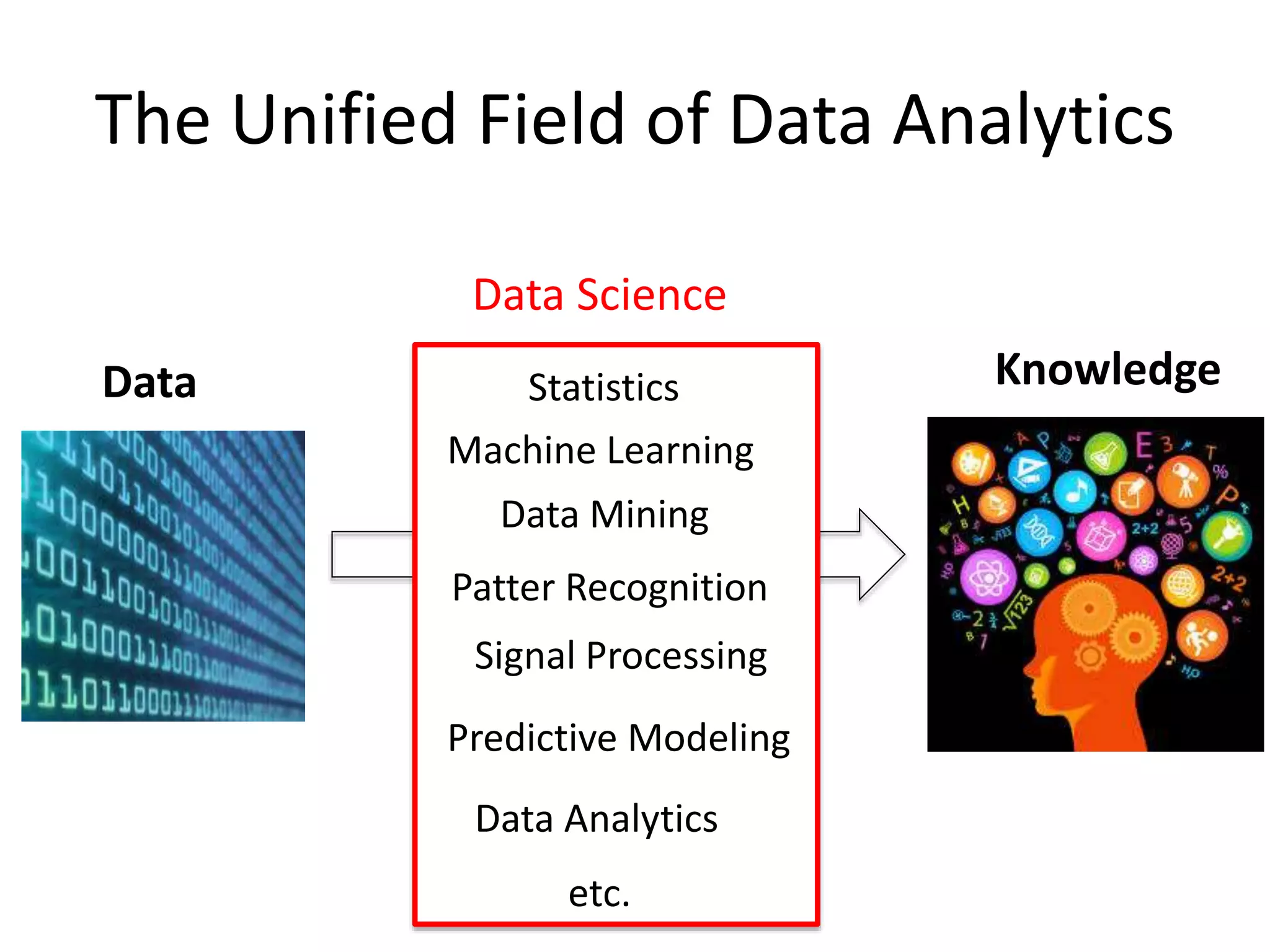
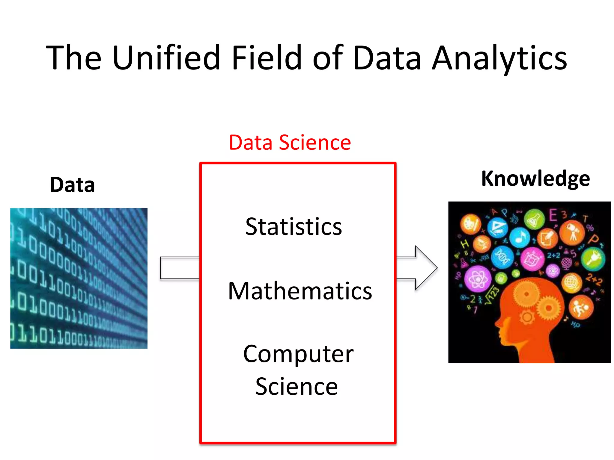
Unified field of data analytics combining statistics, data mining, and machine learning.
Timeline of data science from the 1960s to present; increasing demand for data scientists.
Role and process of a data scientist; steps involved in data analysis.
Definition of Big Data, its dimensions: Volume, Variety, Velocity, and Veracity.
What makes big data possible: advancements in generation, storage, processing, and algorithms. The evolution of storage technology and its impact on data science capabilities.
Benefits and structure of cloud computing for storage and processing of large datasets.
Revolutionary algorithms enabling big data processing, notably MapReduce and Hadoop.
Details on the process, types of data analytics and the significance of machine learning.
Challenges faced in industrializing data science, including data quality, problem definition.
Key skills required to become a data scientist and educational resources available.
Final remarks emphasizing the significance of data, especially big data, for businesses.
Big Data and Data Science: The Technologies Shaping Our Lives
1.
Big Data andData Science: The
Technologies Shaping Our Lives
Dr. Rukshan Batuwita (Machine Learning Scientist)
Senior Data Scientist
Ambiata Pvt Ltd, Sydney, Australia
2.
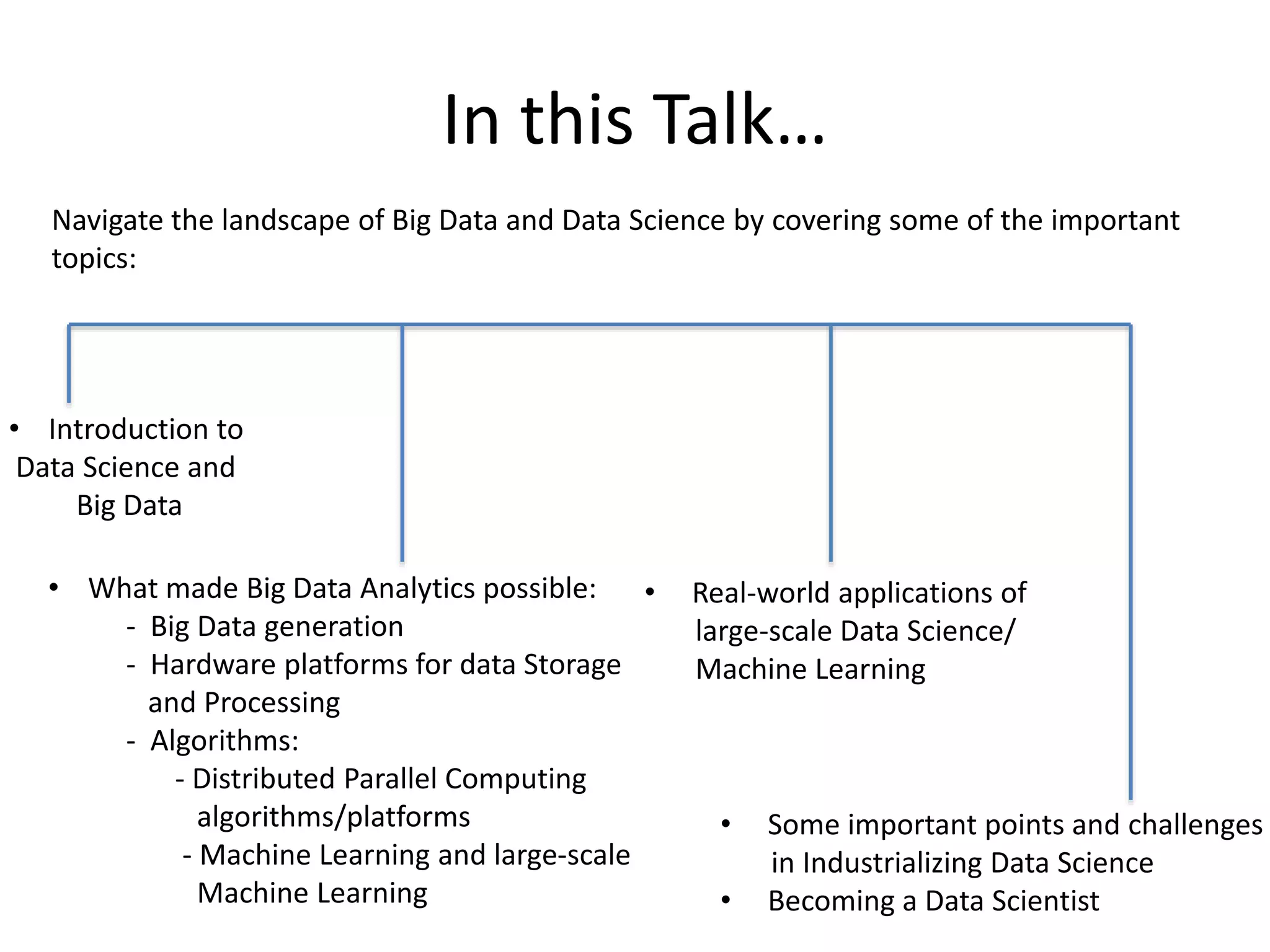
In this Talk…
Navigatethe landscape of Big Data and Data Science by covering some of the important
topics:
• Introduction to
Data Science and
Big Data
• What made Big Data Analytics possible:
- Big Data generation
- Hardware platforms for data Storage
and Processing
- Algorithms:
- Distributed Parallel Computing
algorithms/platforms
- Machine Learning and large-scale
Machine Learning
• Some important points and challenges
in Industrializing Data Science
• Becoming a Data Scientist
• Real-world applications of
large-scale Data Science/
Machine Learning
3.
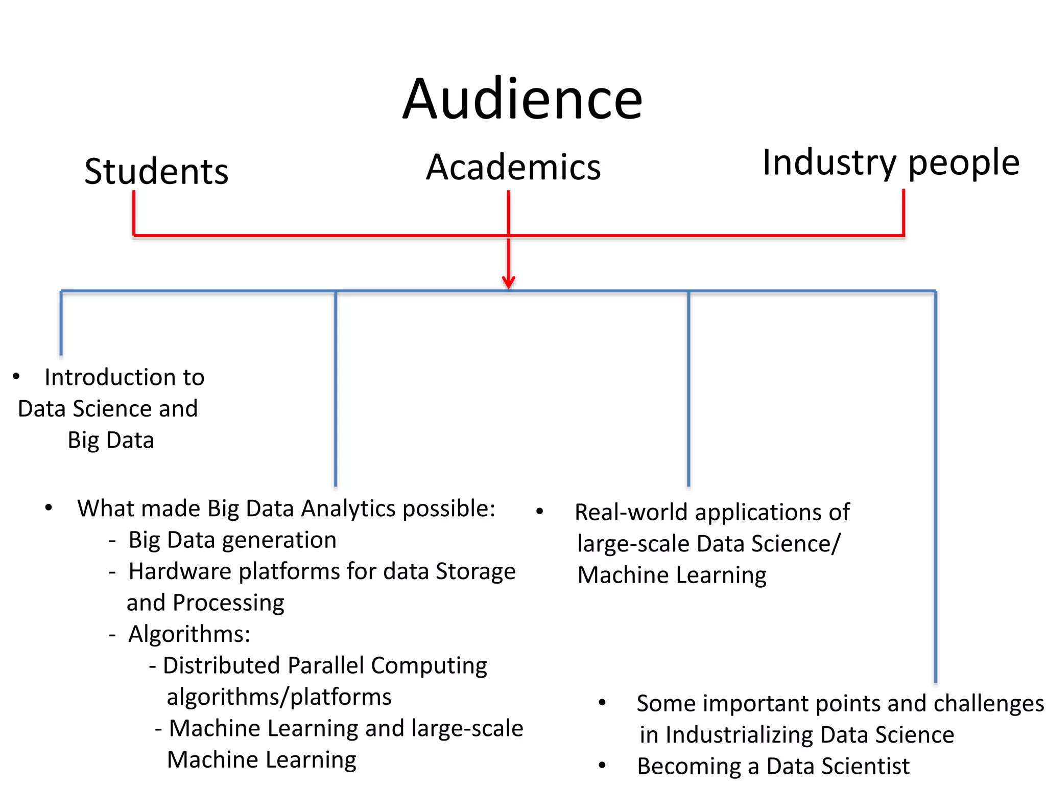
Audience
• Introduction to
DataScience and
Big Data
• What made Big Data Analytics possible:
- Big Data generation
- Hardware platforms for data Storage
and Processing
- Algorithms:
- Distributed Parallel Computing
algorithms/platforms
- Machine Learning and large-scale
Machine Learning
• Some important points and challenges
in Industrializing Data Science
• Becoming a Data Scientist
• Real-world applications of
large-scale Data Science/
Machine Learning
Students Academics Industry people
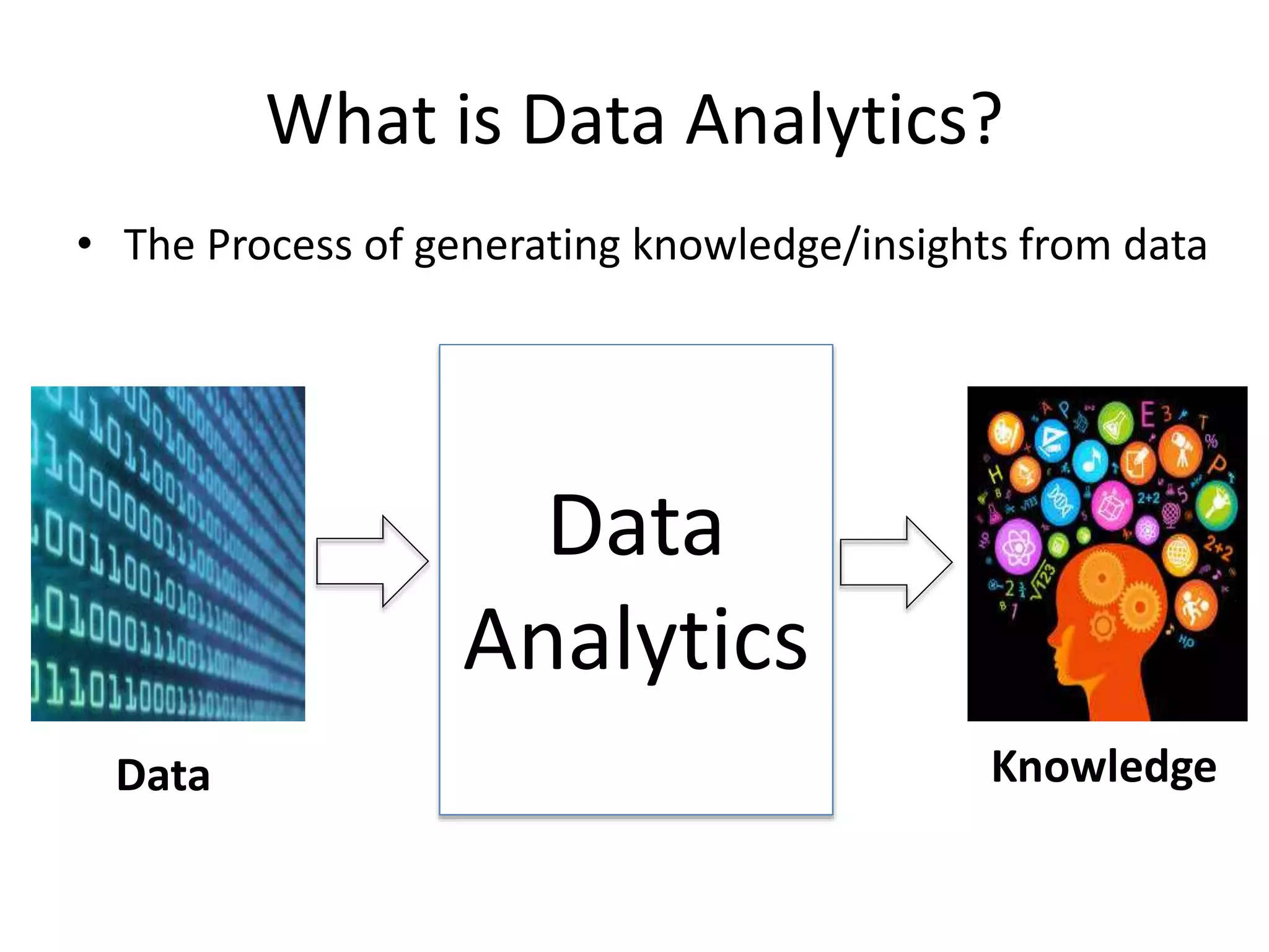
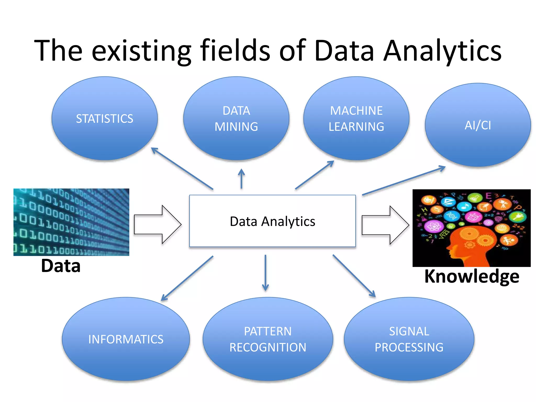
What is DataAnalytics?
• The Process of generating knowledge/insights from data
Data Knowledge
Data
Analytics
6.
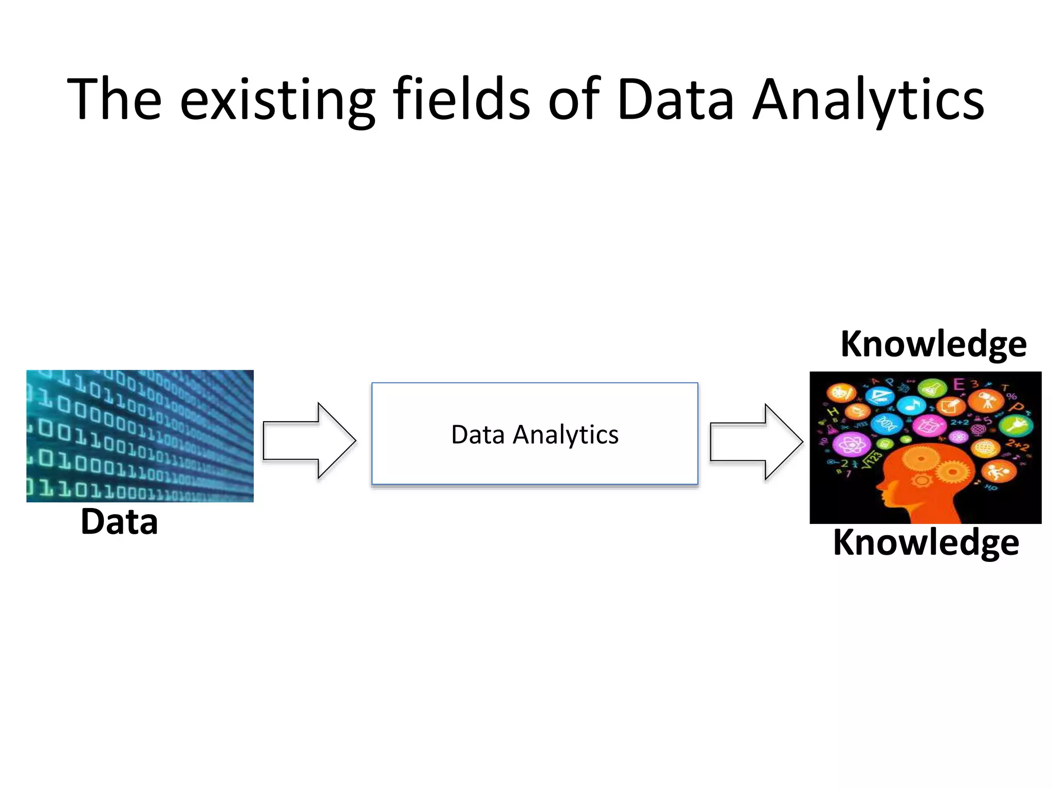
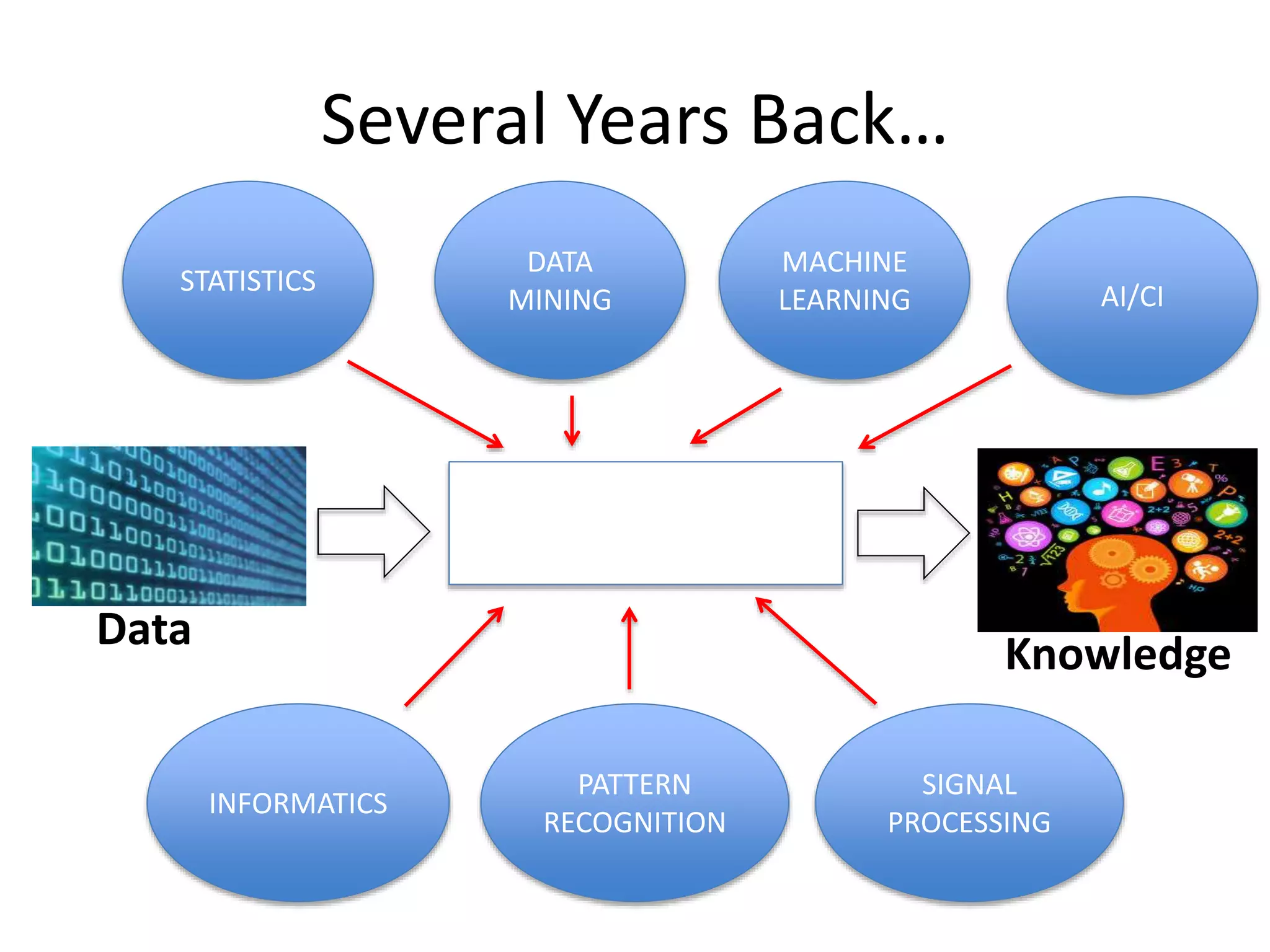
The existing fieldsof Data Analytics
Knowledge
Data
Knowledge
Data Analytics
7.
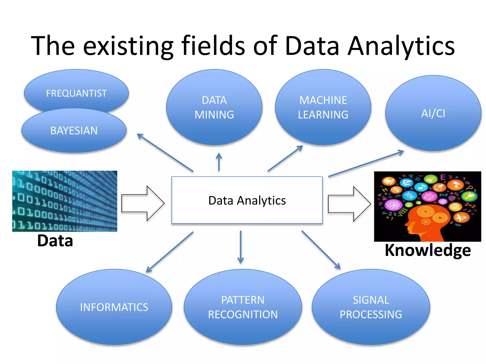
The existing fieldsof Data Analytics
Data
Knowledge
Data Analytics
STATISTICS
PATTERN
RECOGNITION
MACHINE
LEARNING AI/CI
INFORMATICS
DATA
MINING
SIGNAL
PROCESSING
8.
The existing fieldsof Data Analytics
Data
Knowledge
Data Analytics
PATTERN
RECOGNITION
MACHINE
LEARNING AI/CI
INFORMATICS
DATA
MINING
SIGNAL
PROCESSING
FREQUANTIST
BAYESIAN
9.
The existing fieldsof Data Analytics
Data
Knowledge
Data Analytics
STATISTICS
PATTERN
RECOGNITION
MACHINE
LEARNING AI/CI
INFORMATICS
DATA
MINING
SIGNAL
PROCESSING
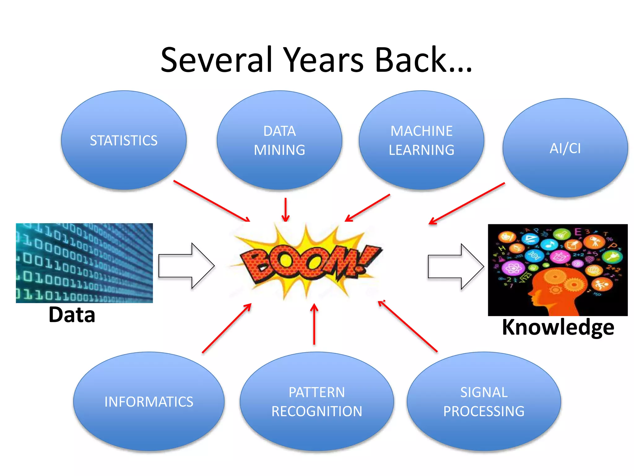
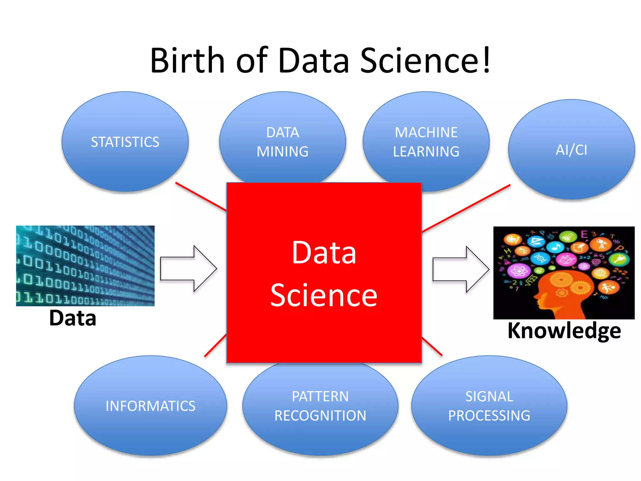
The Unified Fieldof Data Analytics
Machine Learning
Data Mining
Statistics
Patter Recognition
Signal Processing
Predictive Modeling
Data Knowledge
Data Science
Data Analytics
etc.
15.
The Unified Fieldof Data Analytics
Statistics
Data Knowledge
Data Science
Mathematics
Computer
Science
16.
Data Science
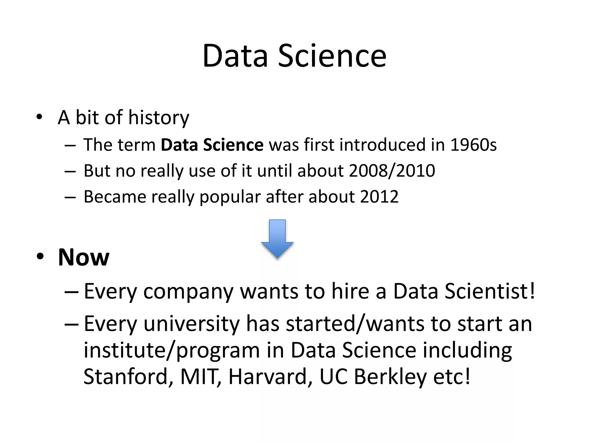
• Abit of history:
– The term “Data Science” was first introduced in
1960s
– But no really use of it until about 2008/2010
– Became really popular after about 2012
17.
Data Science
• Abit of history
– The term Data Science was first introduced in 1960s
– But no really use of it until about 2008/2010
– Became really popular after about 2012
• Now
– Every company wants to hire a Data Scientist!
– Every university has started/wants to start an
institute/program in Data Science including
Stanford, MIT, Harvard, UC Berkley etc!
18.
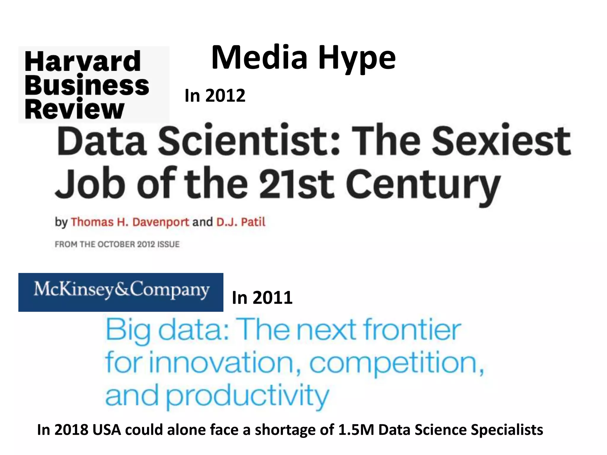
Media Hype
In 2012
In2011
In 2018 USA could alone face a shortage of 1.5M Data Science Specialists
19.
The Data Scientist?
•The person who is involved in the Data
Science process
Data KnowledgeData Scientist
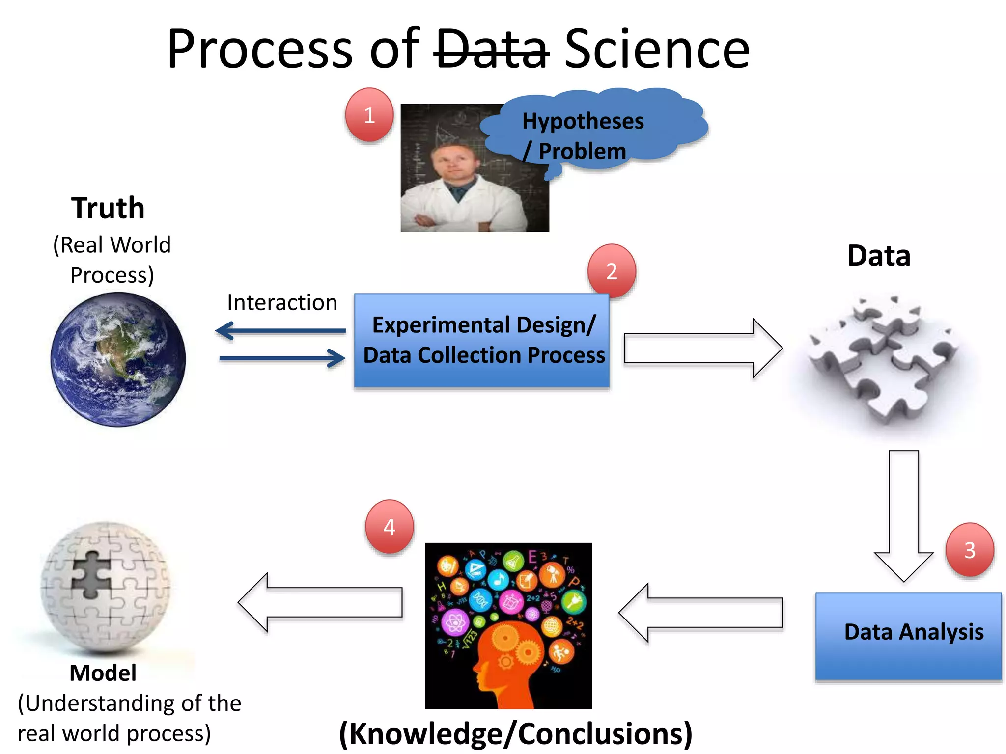
Process of DataScience
Truth
(Knowledge/Conclusions)
Data
Experimental Design/
Data Collection Process
Data Analysis
(Real World
Process)
Interaction
1
2
3
Model
(Understanding of the
real world process)
4
Hypotheses
/ Problem
22.
Process of DataScience
Truth
(Knowledge/Conclusions)
Data
Hypotheses
/ Problem
Data Analysis
(Real World
Process)
Interaction
1
2
3
Model
(Understanding of the
real world process)
4
Experimental Design/
Data Collection Process
23.
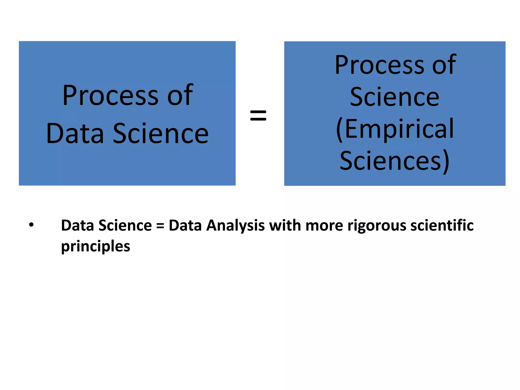
Process of
Data Science
Processof
Science
(Empirical
Sciences)
=
• Data Science = Data Analysis with more rigorous scientific
principles
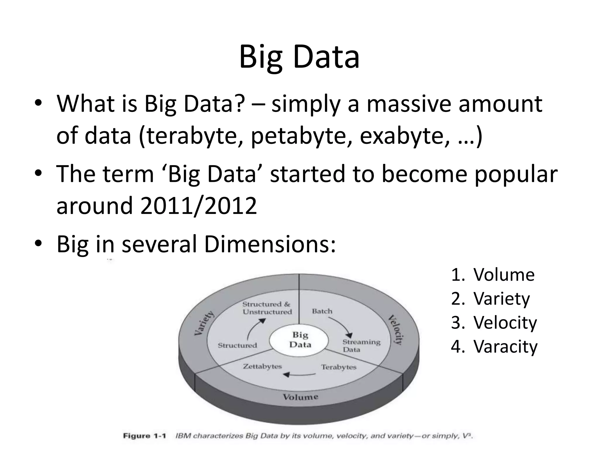
Big Data
• Whatis Big Data? – simply a massive amount
of data (terabyte, petabyte, exabyte, …)
• The term ‘Big Data’ started to become popular
around 2011/2012
• Big in several Dimensions:
1. Volume
2. Variety
3. Velocity
4. Varacity
What made BigData
Possible?
1. Advancements in
Data Generation
28.
Advancements in DataGeneration
• Advancement of Science and Technology:
• Everyday we create about 2.5 Quintillion (1018) bytes of data*
• Every event we do generates data: search, click, like, email,
message, etc.
Internet:
* http://www-01.ibm.com/software/data/bigdata/what-is-big-data.html
350M photos added each day
29.
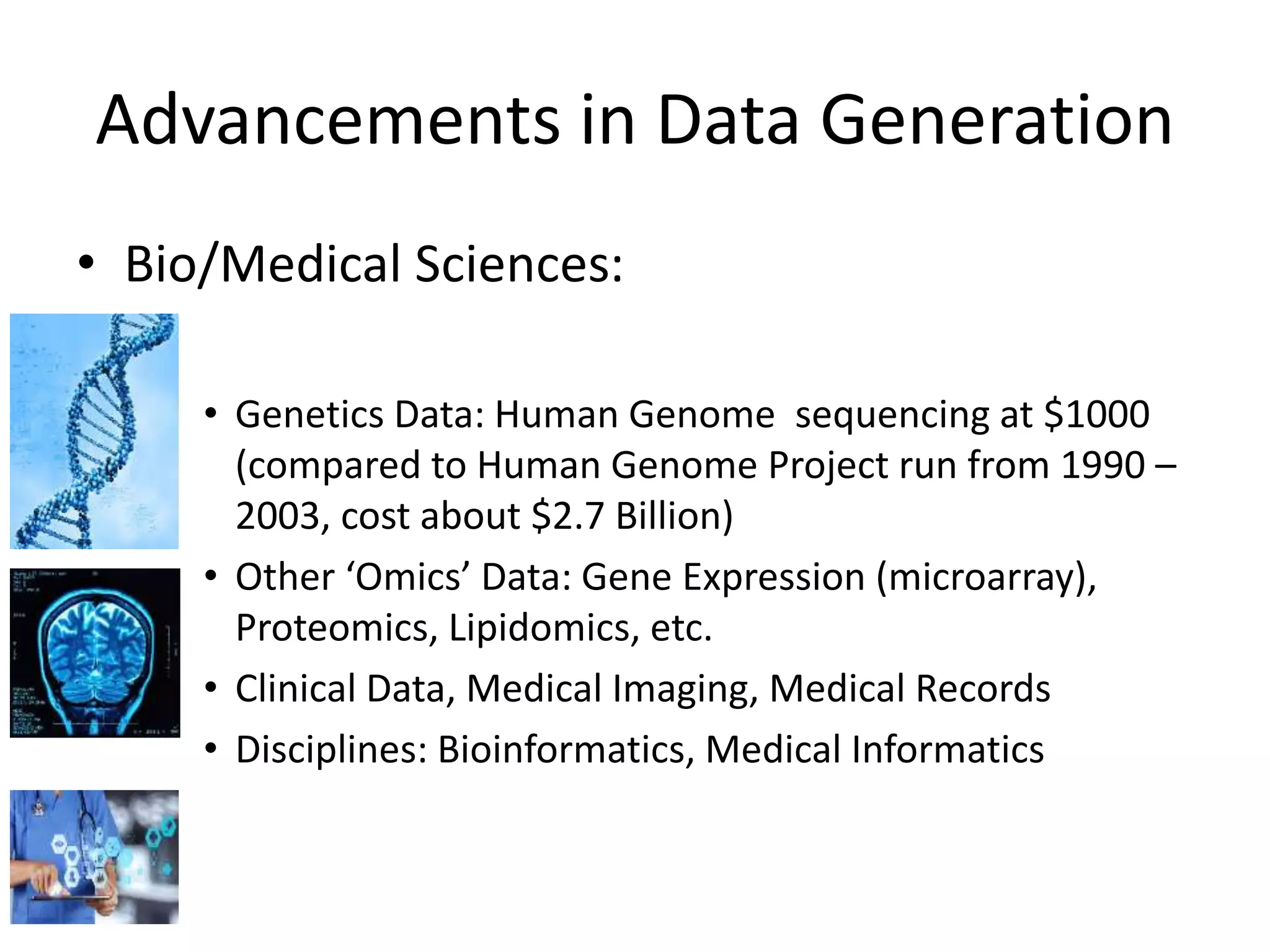
• Bio/Medical Sciences:
•Genetics Data: Human Genome sequencing at $1000
(compared to Human Genome Project run from 1990 –
2003, cost about $2.7 Billion)
• Other ‘Omics’ Data: Gene Expression (microarray),
Proteomics, Lipidomics, etc.
• Clinical Data, Medical Imaging, Medical Records
• Disciplines: Bioinformatics, Medical Informatics
Advancements in Data Generation
30.
Advancements in DataGeneration
• Astronomy
• Physics
SETI project:
Large Hadron Collider – 50 TB per day
Hubble Telescope Largest Radio Telescope
TB/PB of Data each day
31.
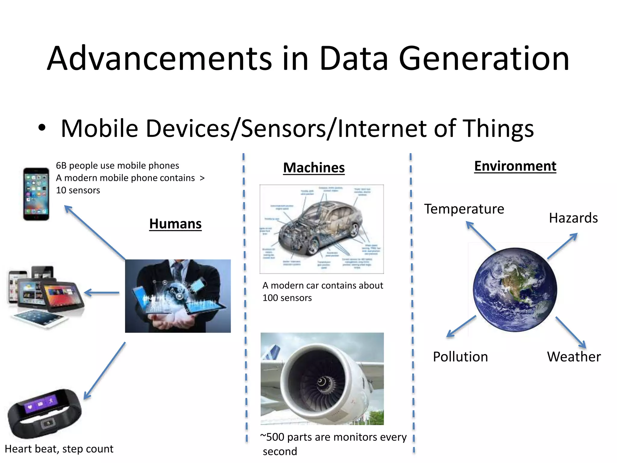
Advancements in DataGeneration
• Mobile Devices/Sensors/Internet of Things
6B people use mobile phones
A modern mobile phone contains >
10 sensors
Heart beat, step count
Machines
A modern car contains about
100 sensors
~500 parts are monitors every
second
Environment
Pollution Weather
Temperature
HazardsHumans
32.
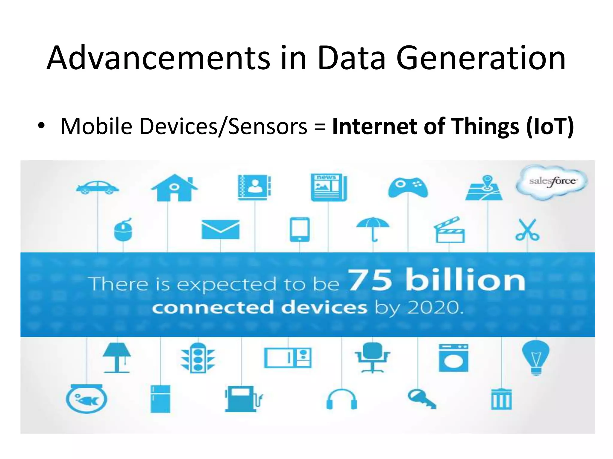
Advancements in DataGeneration
• Mobile Devices/Sensors = Internet of Things (IoT)
33.
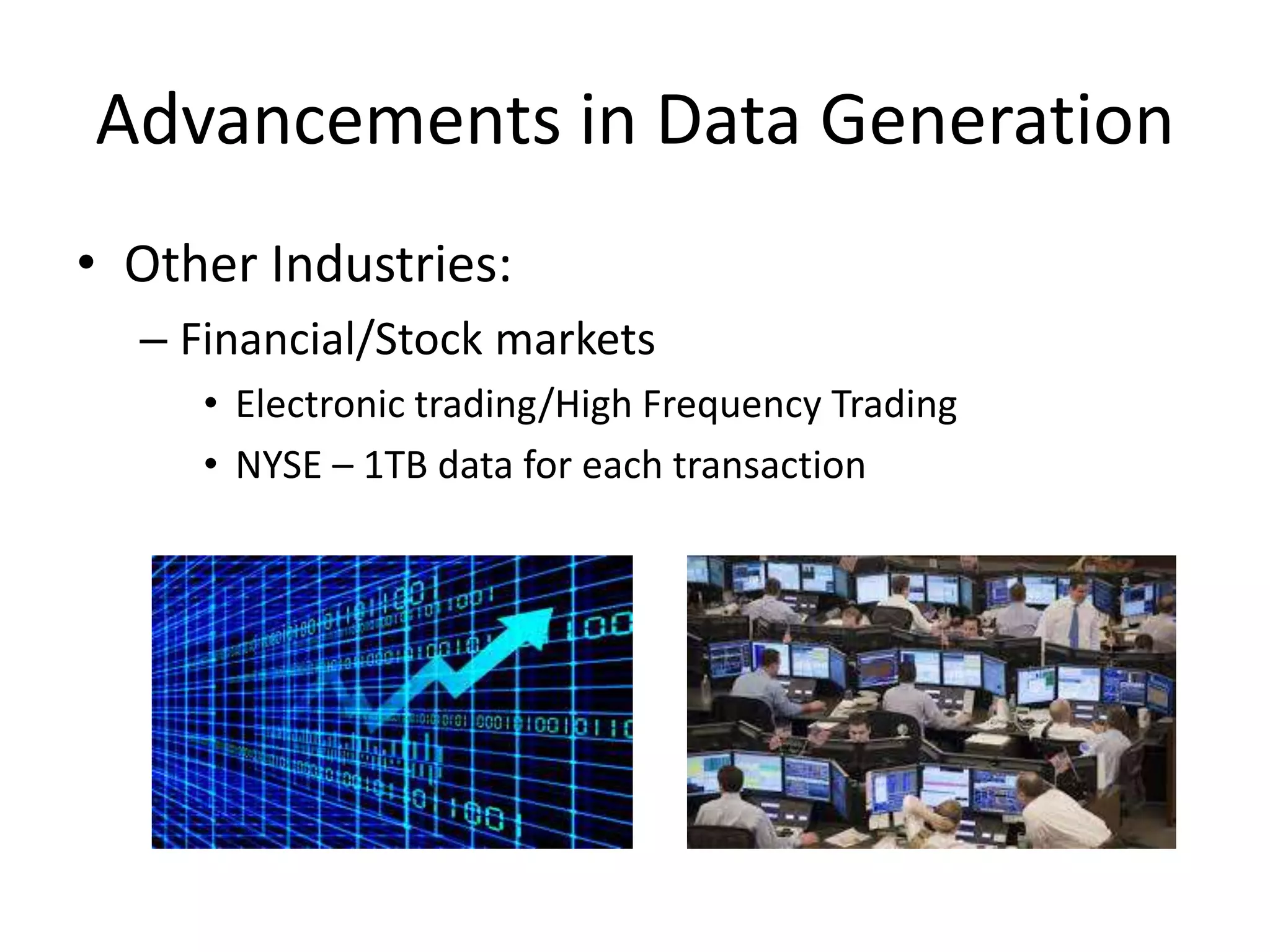
• Other Industries:
–Financial/Stock markets
• Electronic trading/High Frequency Trading
• NYSE – 1TB data for each transaction
Advancements in Data Generation
34.
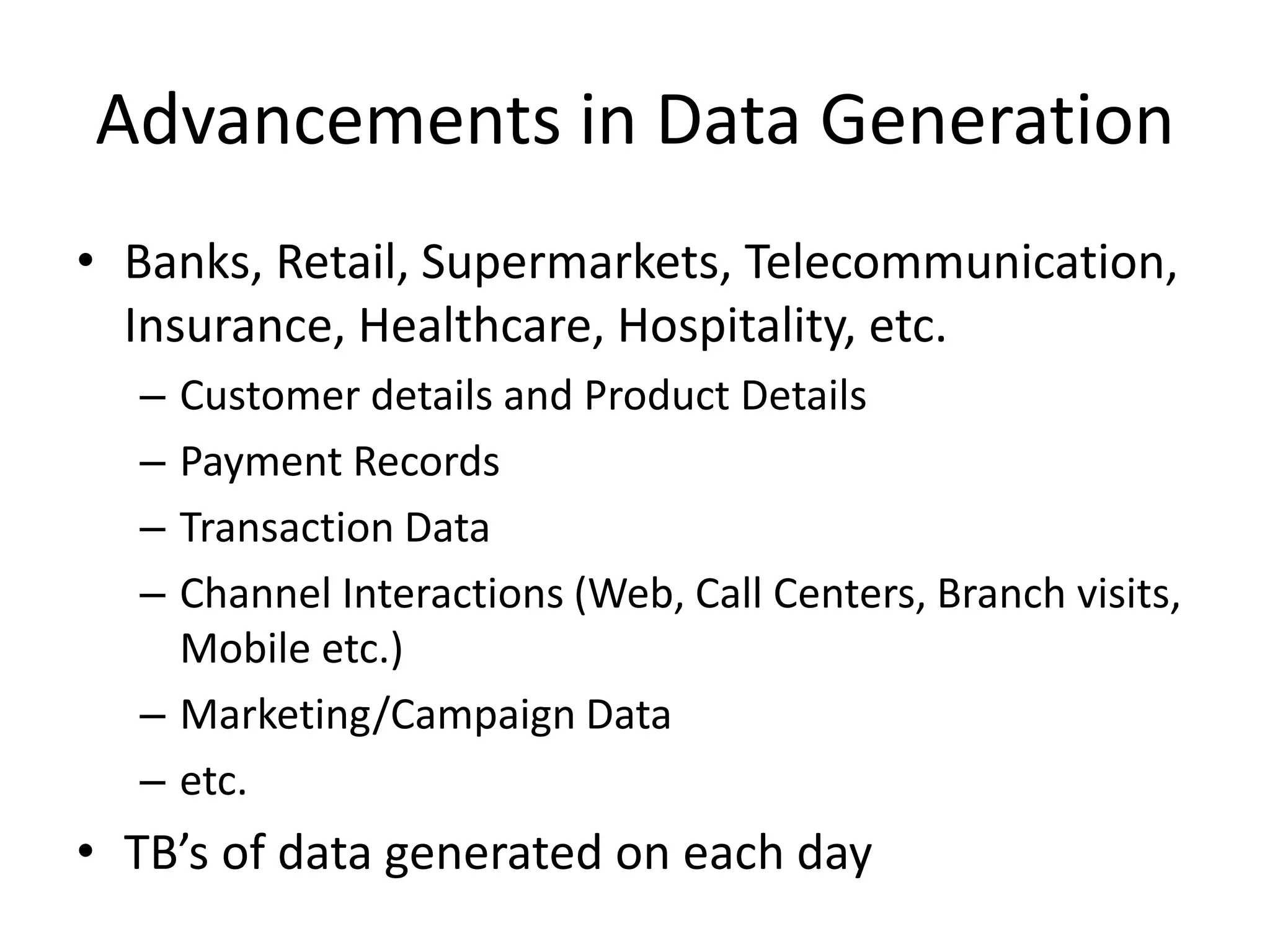
• Banks, Retail,Supermarkets, Telecommunication,
Insurance, Healthcare, Hospitality, etc.
– Customer details and Product Details
– Payment Records
– Transaction Data
– Channel Interactions (Web, Call Centers, Branch visits,
Mobile etc.)
– Marketing/Campaign Data
– etc.
• TB’s of data generated on each day
Advancements in Data Generation
35.
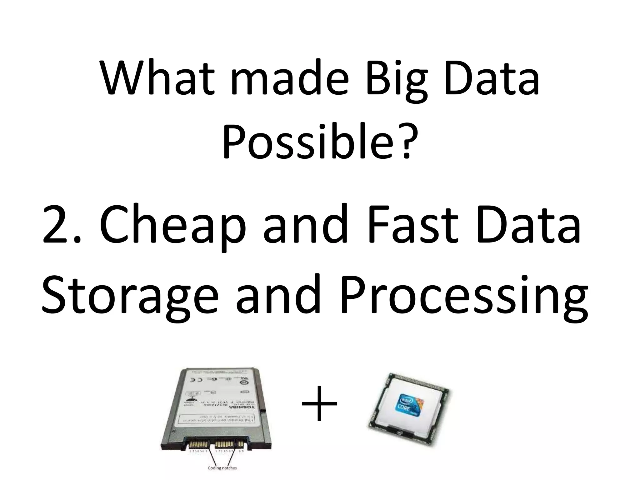
What made BigData
Possible?
2. Cheap and Fast Data
Storage and Processing
36.
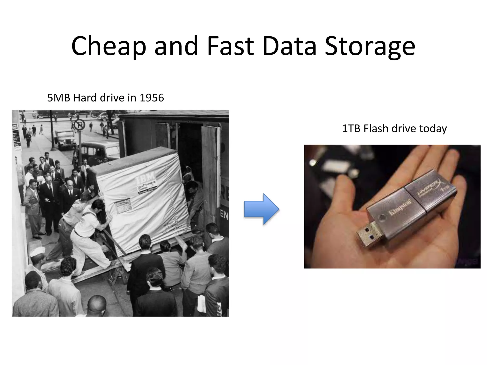
Cheap and FastData Storage
5MB Hard drive in 1956
1TB Flash drive today
37.
Cheap and FastData Storage
http://www.mkomo.com/cost-per-gigabyte
Several Hundred Thousands
A couple of cents
38.
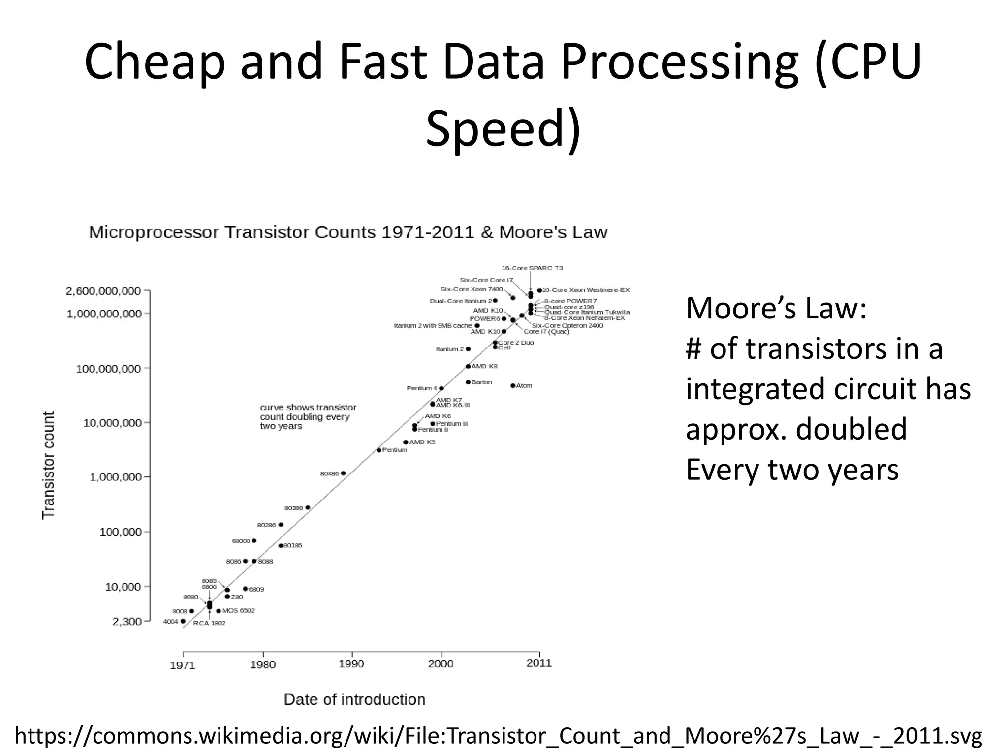
Cheap and FastData Processing (CPU
Speed)
Moore’s Law:
# of transistors in a
integrated circuit has
approx. doubled
Every two years
https://commons.wikimedia.org/wiki/File:Transistor_Count_and_Moore%27s_Law_-_2011.svg
39.
Cheap and FastData Processing (CPU
Speed)
https://ourworldindata.org/technological-progress/
40.
Cheap and FastStorage and
Processing
State-of-the-Art
Computing Systems
41.
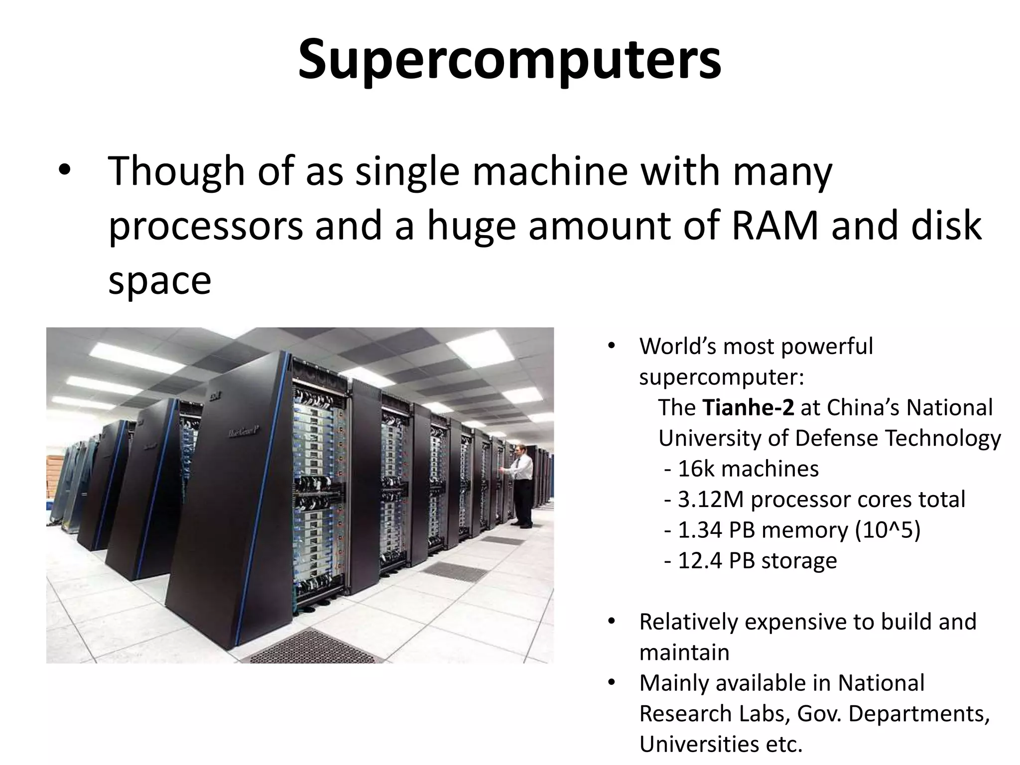
Supercomputers
• Though ofas single machine with many
processors and a huge amount of RAM and disk
space
• World’s most powerful
supercomputer:
The Tianhe-2 at China’s National
University of Defense Technology
- 16k machines
- 3.12M processor cores total
- 1.34 PB memory (10^5)
- 12.4 PB storage
• Relatively expensive to build and
maintain
• Mainly available in National
Research Labs, Gov. Departments,
Universities etc.
42.
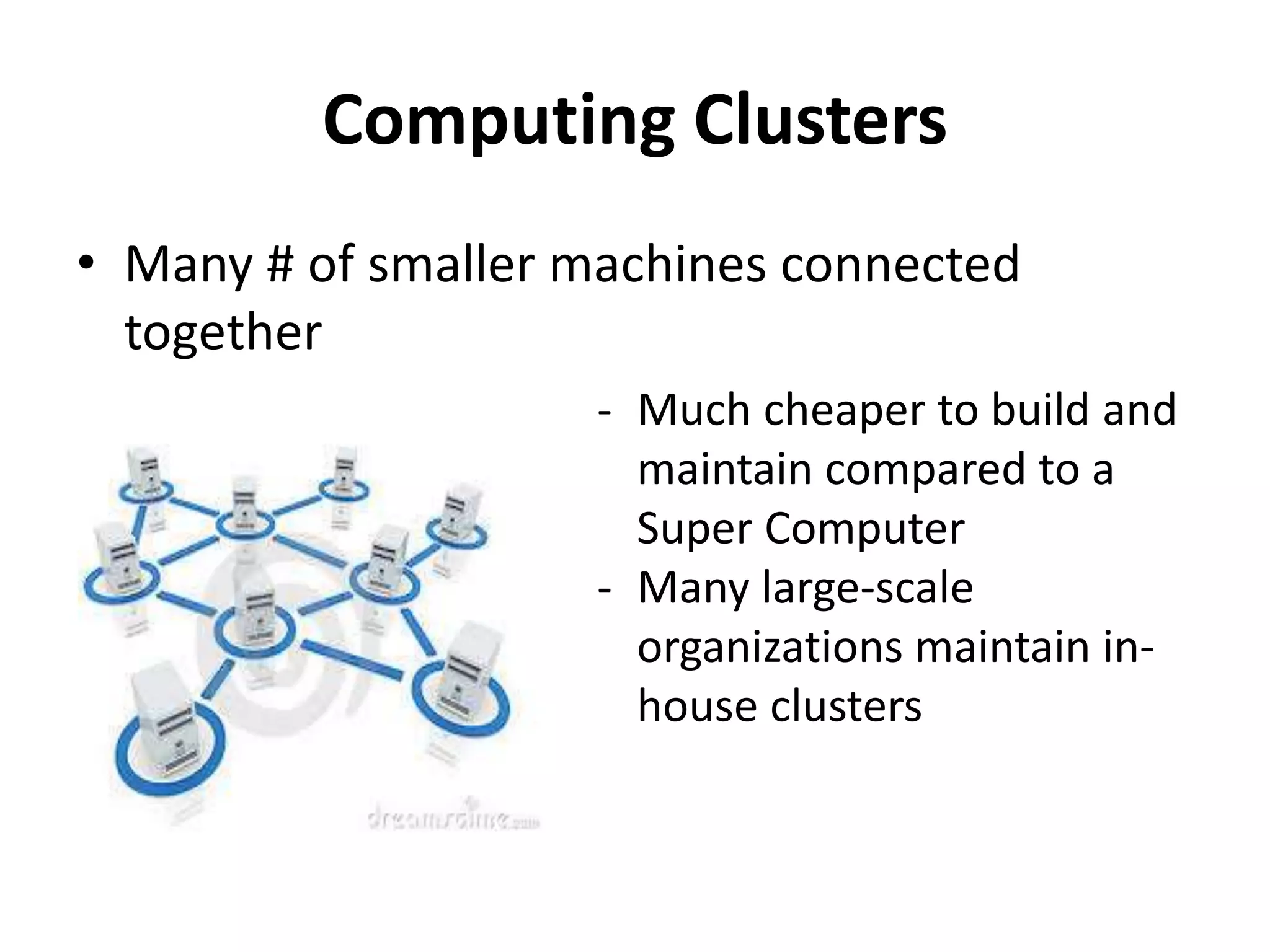
Computing Clusters
• Many# of smaller machines connected
together
- Much cheaper to build and
maintain compared to a
Super Computer
- Many large-scale
organizations maintain in-
house clusters
43.
GPU Computing
• Useof Graphical Processing Units for computing
• NVIDA is one of the main manufactures of GPUs
• CUDA is a parallel computing platform for GPUs by NVIDA
44.
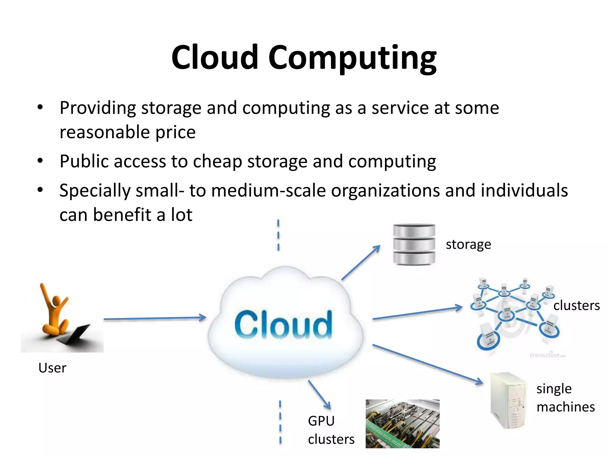
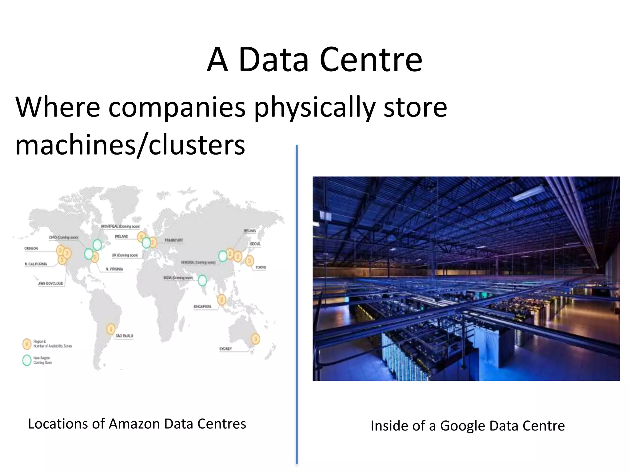
Cloud Computing
• Providingstorage and computing as a service at some
reasonable price
• Public access to cheap storage and computing
• Specially small- to medium-scale organizations and individuals
can benefit a lot
storage
clusters
single
machines
GPU
clusters
User
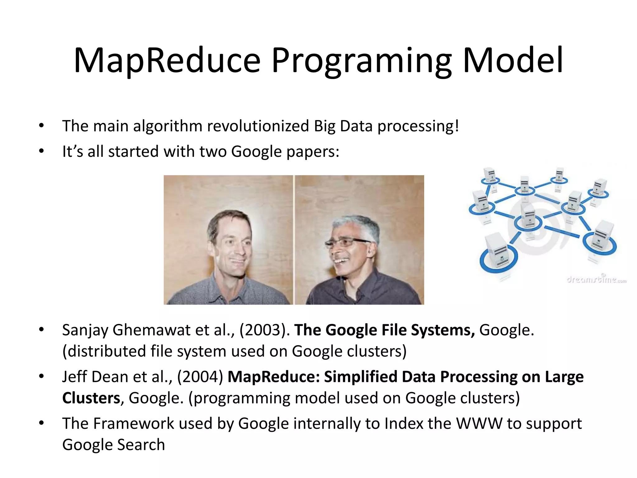
• The mainalgorithm revolutionized Big Data processing!
• It’s all started with two Google papers:
• Sanjay Ghemawat et al., (2003). The Google File Systems, Google.
(distributed file system used on Google clusters)
• Jeff Dean et al., (2004) MapReduce: Simplified Data Processing on Large
Clusters, Google. (programming model used on Google clusters)
• The Framework used by Google internally to Index the WWW to support
Google Search
MapReduce Programing Model
52.
MapReduce Programing Model
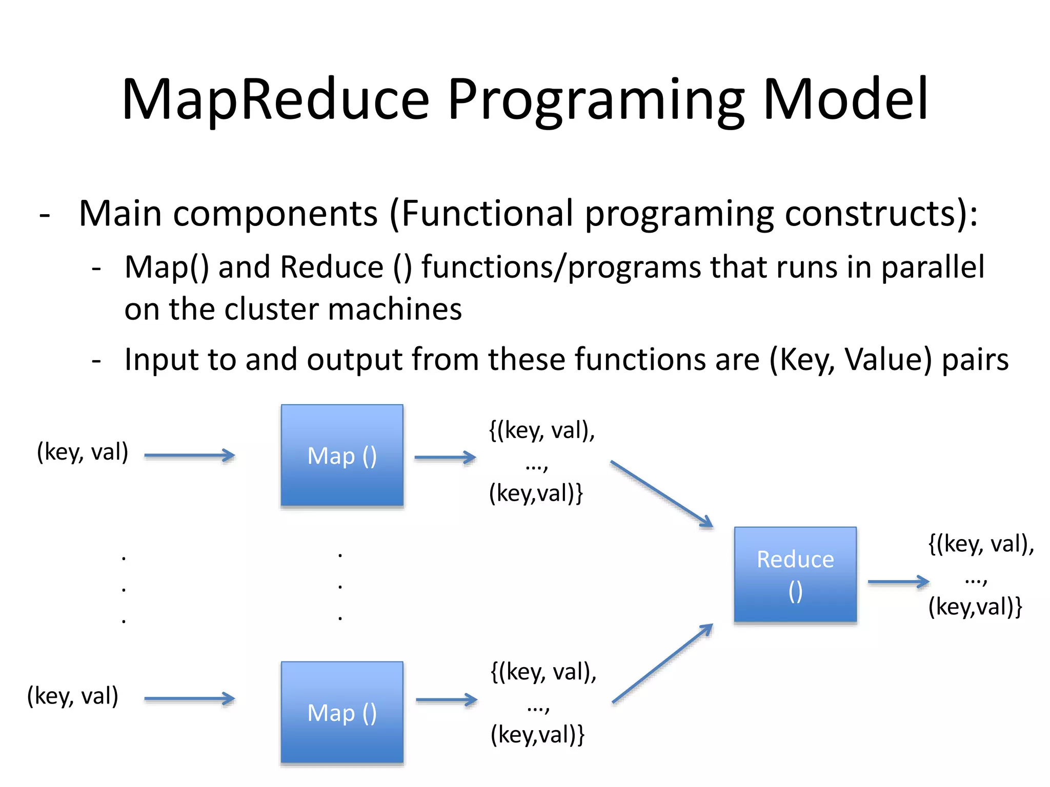
-Main components (Functional programing constructs):
- Map() and Reduce () functions/programs that runs in parallel
on the cluster machines
- Input to and output from these functions are (Key, Value) pairs
Map ()
Reduce
()
(key, val)
Map ()
.
.
.
{(key, val),
…,
(key,val)}
(key, val)
{(key, val),
…,
(key,val)}
{(key, val),
…,
(key,val)}
.
.
.
53.
MapReduce Programing Model
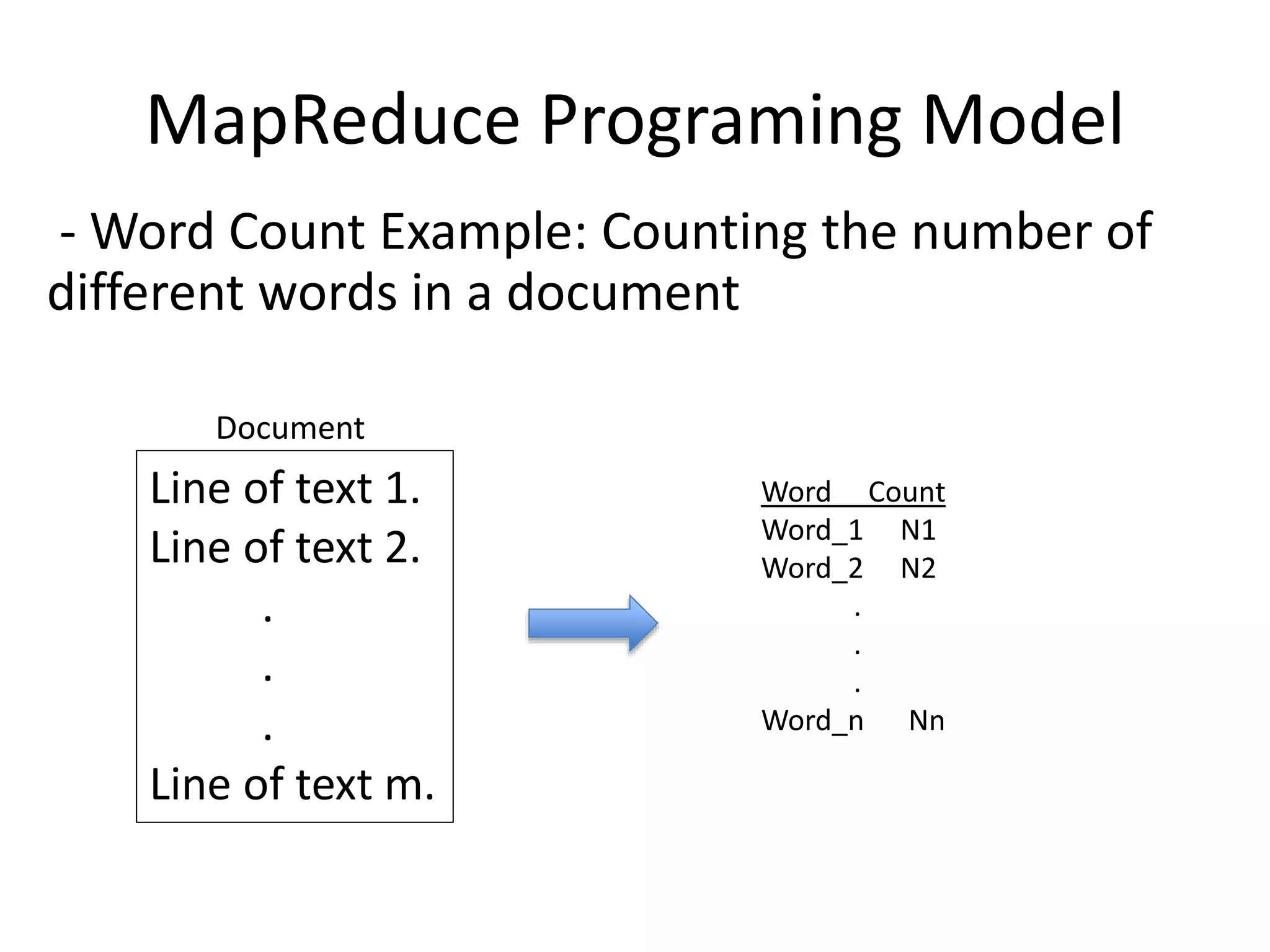
-Word Count Example: Counting the number of
different words in a document
Line of text 1.
Line of text 2.
.
.
.
Line of text m.
Document
Word Count
Word_1 N1
Word_2 N2
.
.
.
Word_n Nn
Apache Hadoop
• ApacheHadoop is the open source implementation of GFS
and MapReduce model
Doug Cutting initiated
The Apache project
Doug Cutting adds DFS and
MapReduce support to Nutch
Yahoo! Releases
first version
Of Hadoop in 2006!
Running Hadoop
on 1000 node cluster
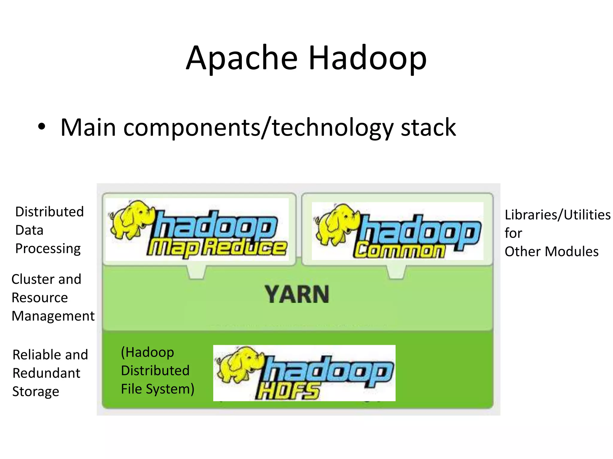
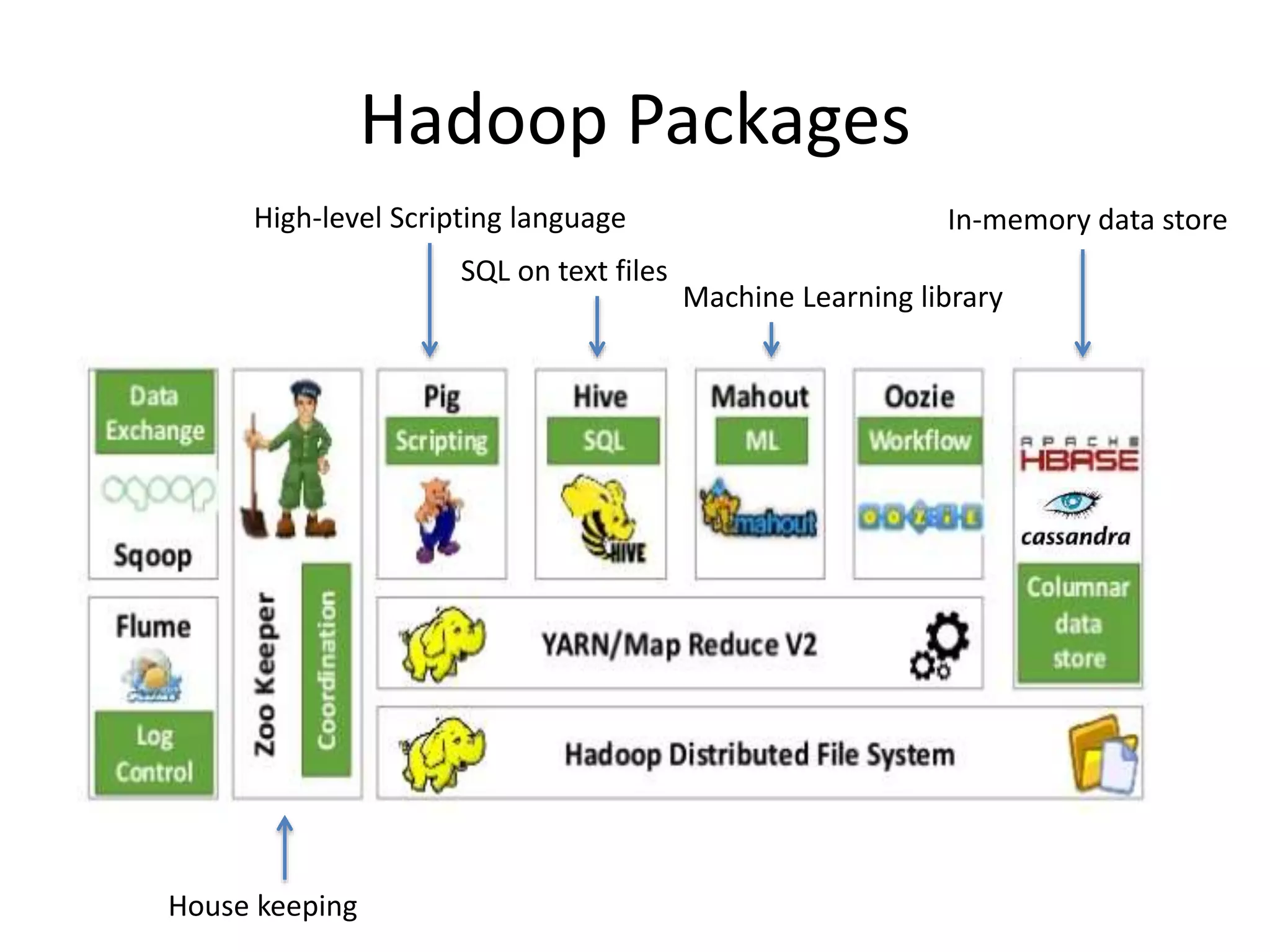
• Main components/technologystack
Apache Hadoop
(Hadoop
Distributed
File System)
Distributed
Data
Processing
Reliable and
Redundant
Storage
Cluster and
Resource
Management
Libraries/Utilities
for
Other Modules
59.
How does Hadoopwork?
• Assume we have a computing cluster where
Hadoop is installed
YARN
Code:
Map()
Reduce()
DataAA
T
A
D
A
Resource
Manager
60.
How does Hadoopwork?
1. Splits and distributes data across the cluster
over HDFS as text files (3 copies of data –
reliable storage)
YARN
DataAA
Code:
Map()
Reduce()
Data Data Data Data
Data
Data
Data
Data
Data
Data
Data
Data
Data
Data
Data
Data
T
A
D
A
Resource
Manager
61.
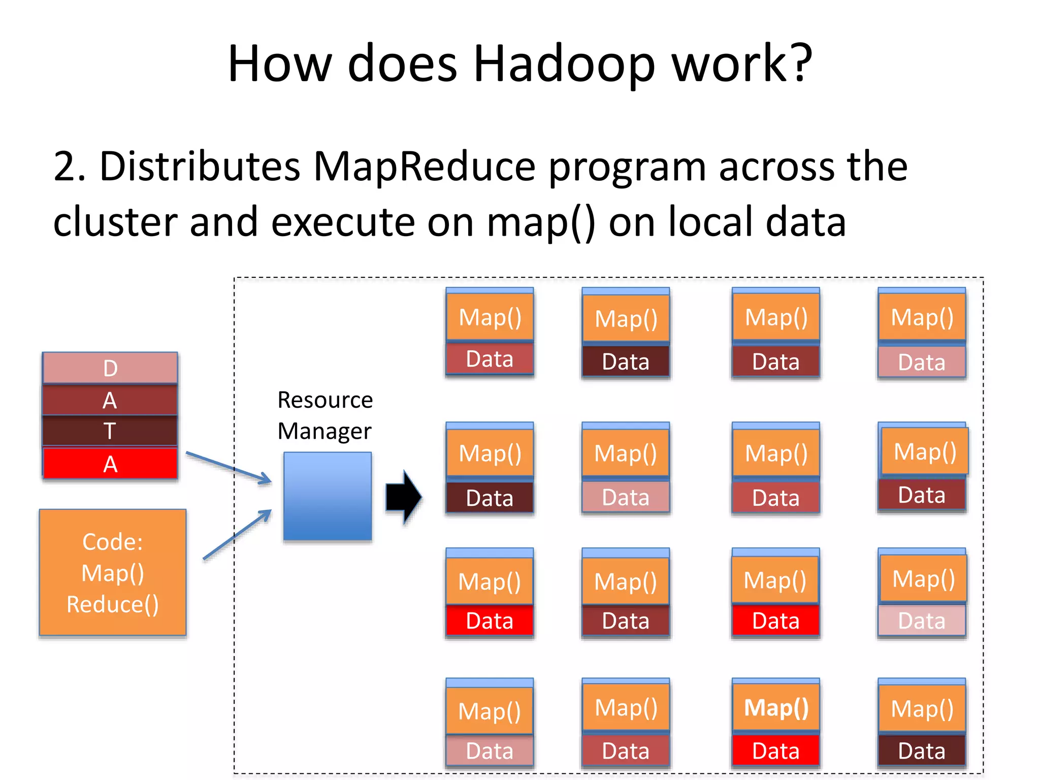
How does Hadoopwork?
2. Distributes MapReduce program across the
cluster and execute on map() on local data
DataAA
Code:
Map()
Reduce()
Data Data Data Data
Data
Data
Data
Data
Data
Data
Data
Data
Data
Data
Data
Data
T
A
D
A
Map() Map()
Map()
Map()
Map()
Map()
Map() Map()
Map()
Map()
Map()
Map()
Map()
Map()
Map()
Map()
Resource
Manager
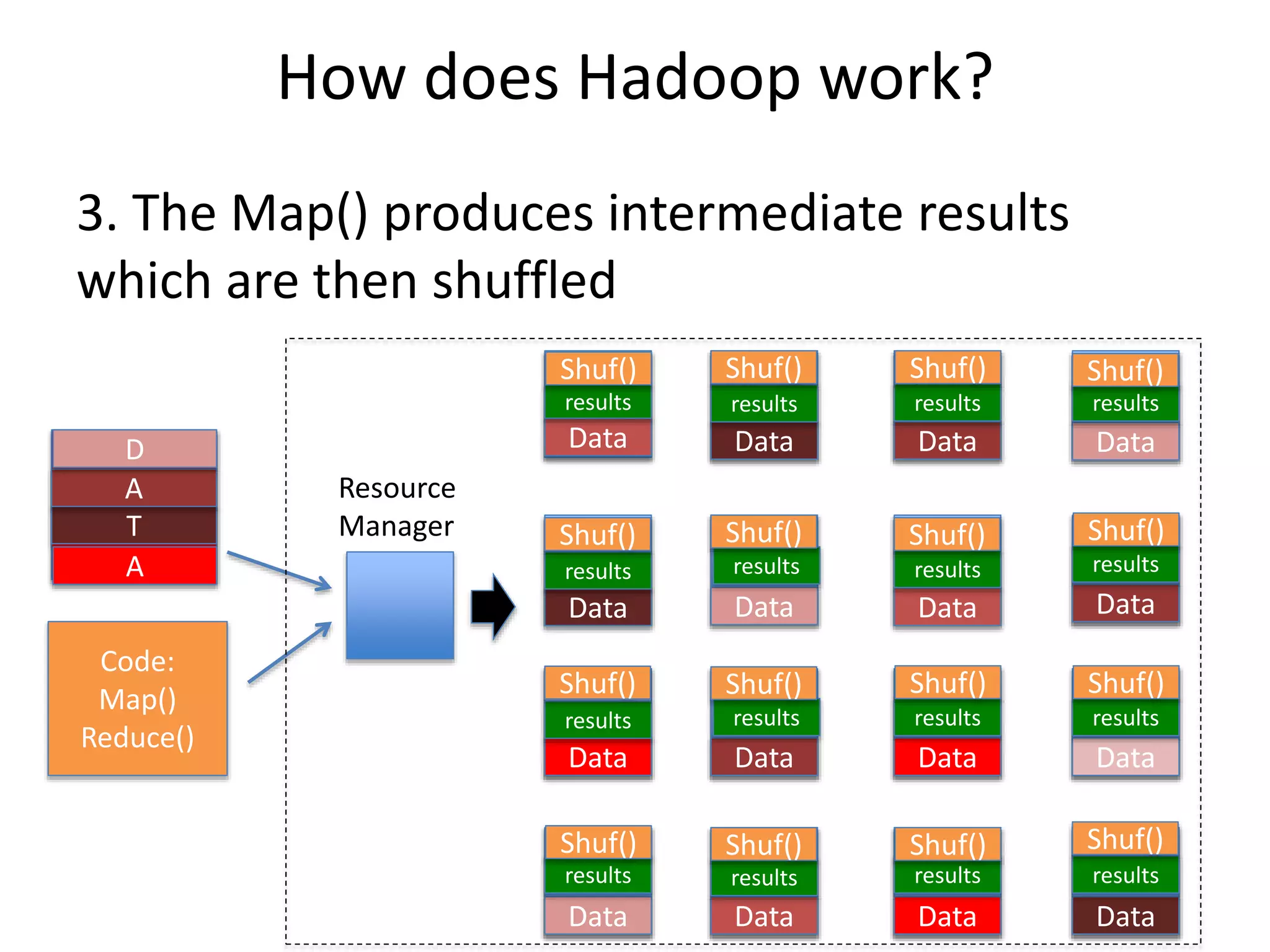
62.
How does Hadoopwork?
3. The Map() produces intermediate results
which are then shuffled
DataAA
Code:
Map()
Reduce()
Data Data Data Data
Data
Data
Data
Data
Data
Data
Data
Data
Data
Data
Data
Data
T
A
D
A
results
results
results
results
results
results
results
results
results
results
results
results
results
results
results
results
Resource
Manager
Shuf() Shuf() Shuf() Shuf()
Shuf()
Shuf()
Shuf() Shuf() Shuf() Shuf()
Shuf() Shuf() Shuf()
Shuf() Shuf() Shuf()
63.
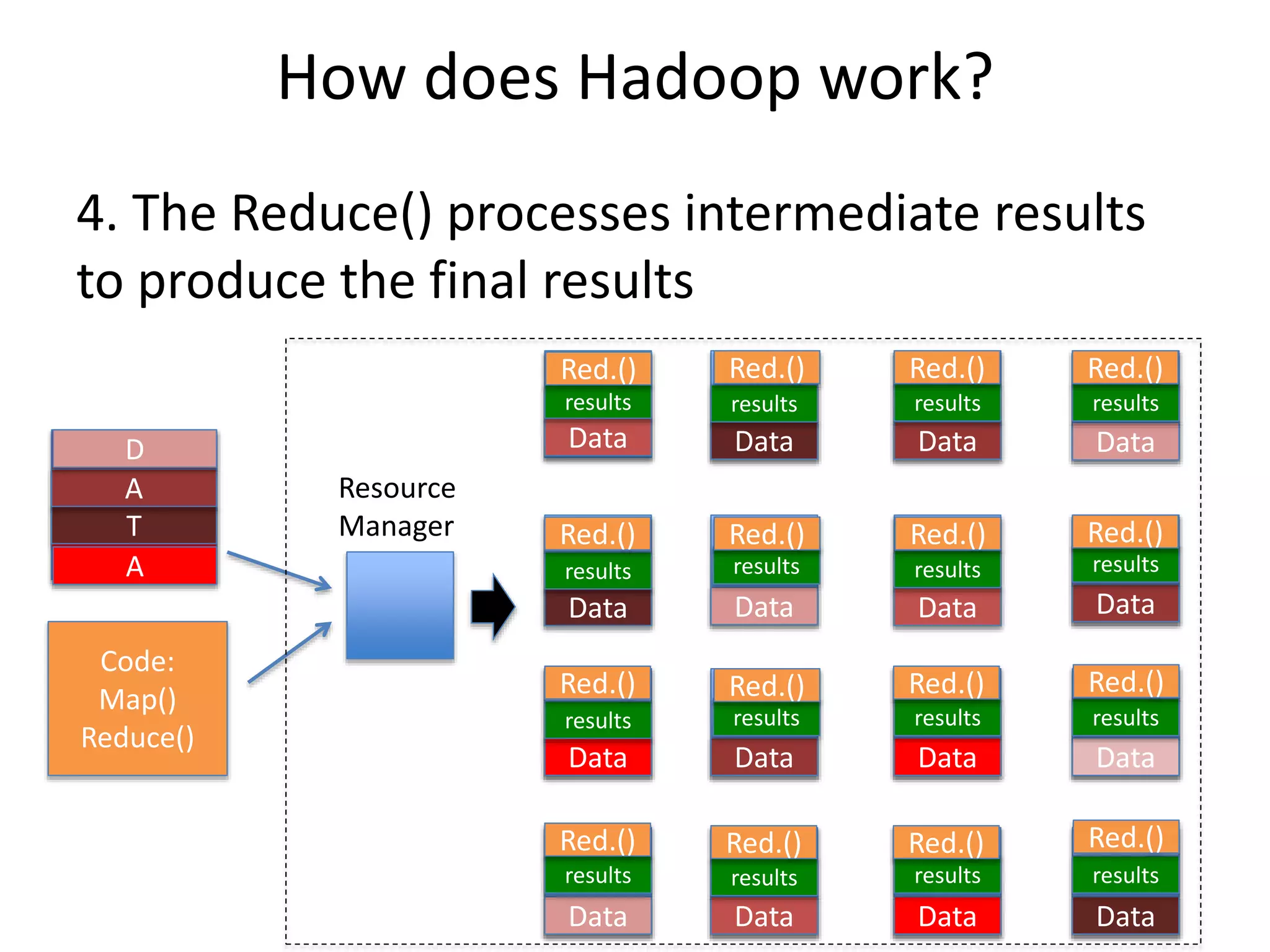
How does Hadoopwork?
4. The Reduce() processes intermediate results
to produce the final results
DataAA
Code:
Map()
Reduce()
Data Data Data Data
Data
Data
Data
Data
Data
Data
Data
Data
Data
Data
Data
Data
T
A
D
A
results
results
results
results
results
results
results
results
results
results
results
results
results
results
results
results
Resource
Manager
Red.() Red.() Red.() Red.()
Red.() Red.() Red.() Red.()
Red.() Red.() Red.() Red.()
Red.() Red.() Red.() Red.()
64.
How does Hadoopwork?
5. Final results are written to HDFS, which can
be collected via the edge node.
DataAA
Code:
Map()
Reduce()
Data Data Data Data
Data
Data
Data
Data
Data
Data
Data
Data
Data
Data
Data
Data
T
A
D
A
results
results
results
results
results
results
results
results
results
results
results
results
results
results
results
results
result
s
Resource
Manager
results results results
results results results results
results results results results
results results results results
65.
Fault Tolerance
• Machines/Harddisks fail all the time!
• Multiple copies can recover the failed tasks
DataAA
Code:
Map()
Reduce()
Data Data Data Data
Data
Data
Data
Data
Data
Data
Data
Data
Data
Data
Data
Data
T
A
D
A
Map() Map()
Map()
Map()
Map()
Map()
Map() Map()
Map()
Map()
Map()
Map()
Map()
Map()
Map()
Map()
Resource
Manager
66.
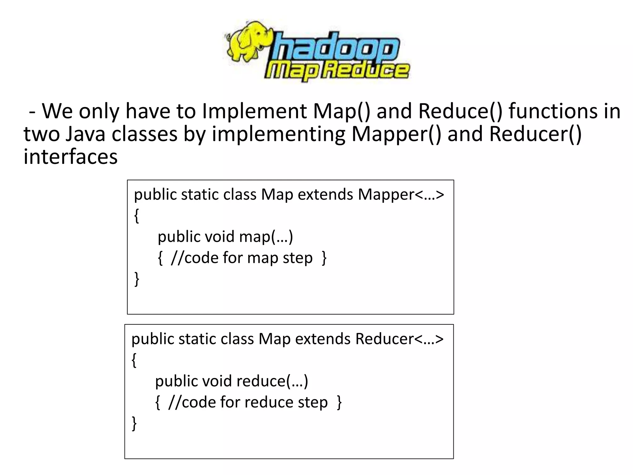
- We onlyhave to Implement Map() and Reduce() functions in
two Java classes by implementing Mapper() and Reducer()
interfaces
public static class Map extends Mapper<…>
{
public void map(…)
{ //code for map step }
}
public static class Map extends Reducer<…>
{
public void reduce(…)
{ //code for reduce step }
}
67.
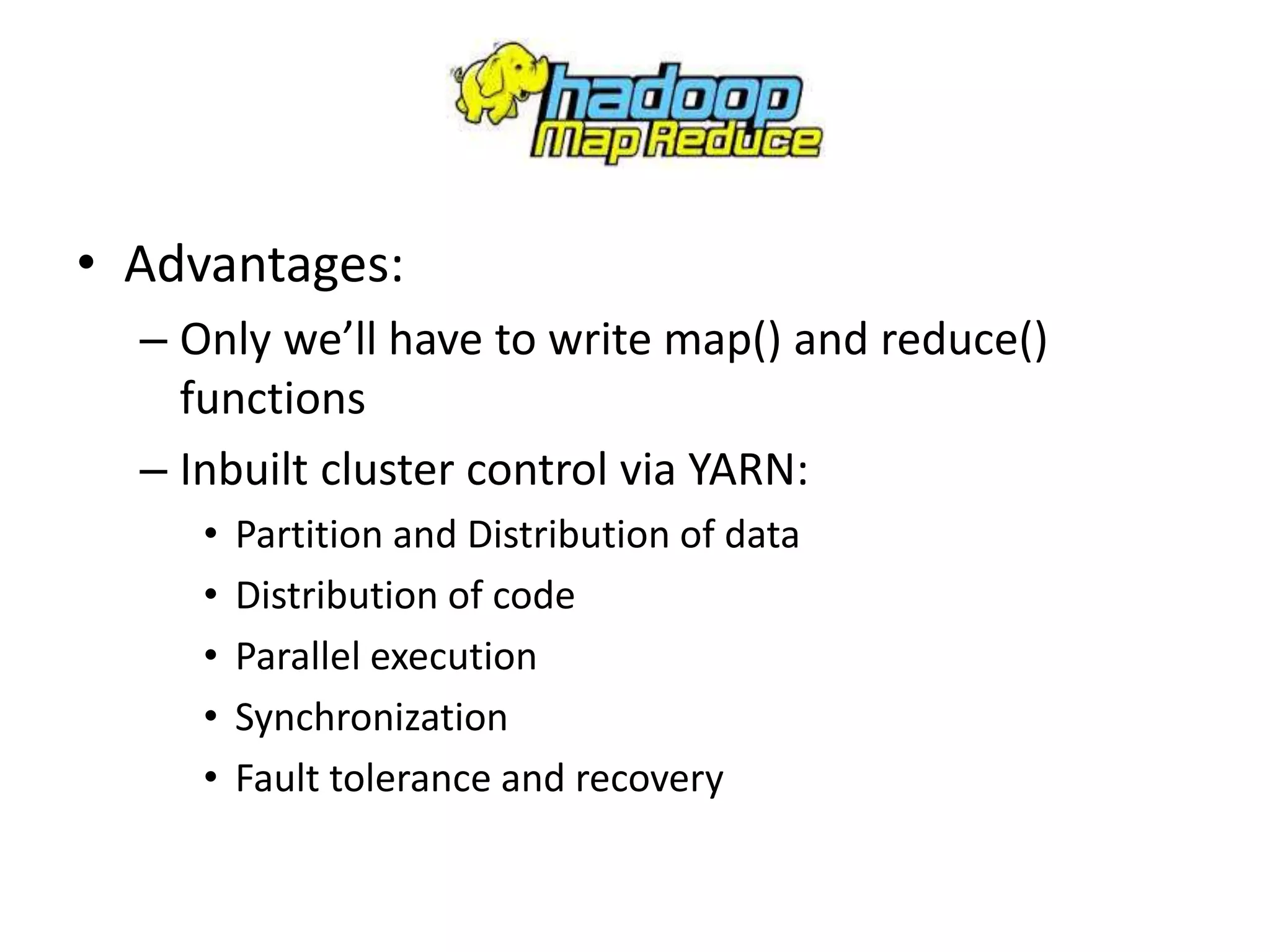
• Advantages:
– Onlywe’ll have to write map() and reduce()
functions
– Inbuilt cluster control via YARN:
• Partition and Distribution of data
• Distribution of code
• Parallel execution
• Synchronization
• Fault tolerance and recovery
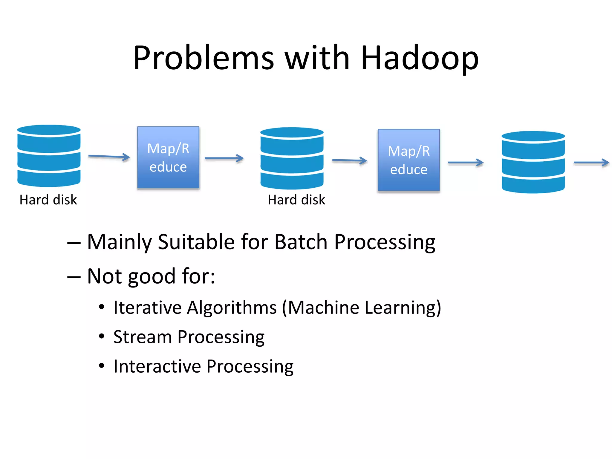
Problems with Hadoop
–Mainly Suitable for Batch Processing
– Not good for:
• Iterative Algorithms (Machine Learning)
• Stream Processing
• Interactive Processing
Map/R
educe
Hard disk Hard disk
Map/R
educe
71.
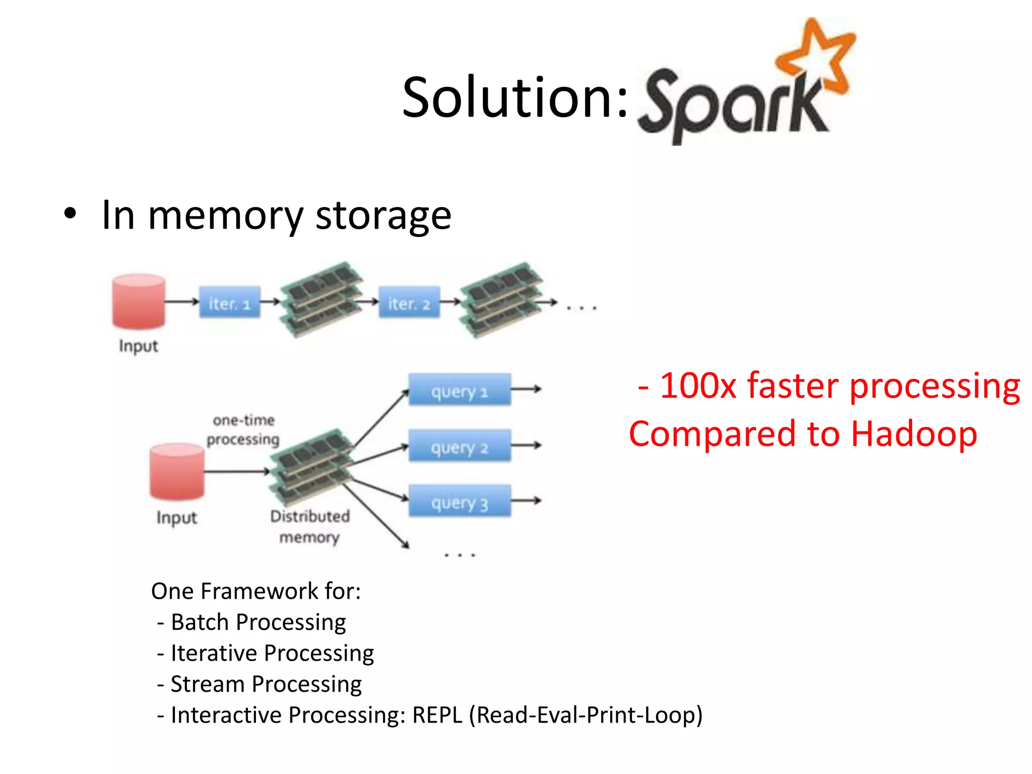
Solution:
• In memorystorage
One Framework for:
- Batch Processing
- Iterative Processing
- Stream Processing
- Interactive Processing: REPL (Read-Eval-Print-Loop)
- 100x faster processing
Compared to Hadoop
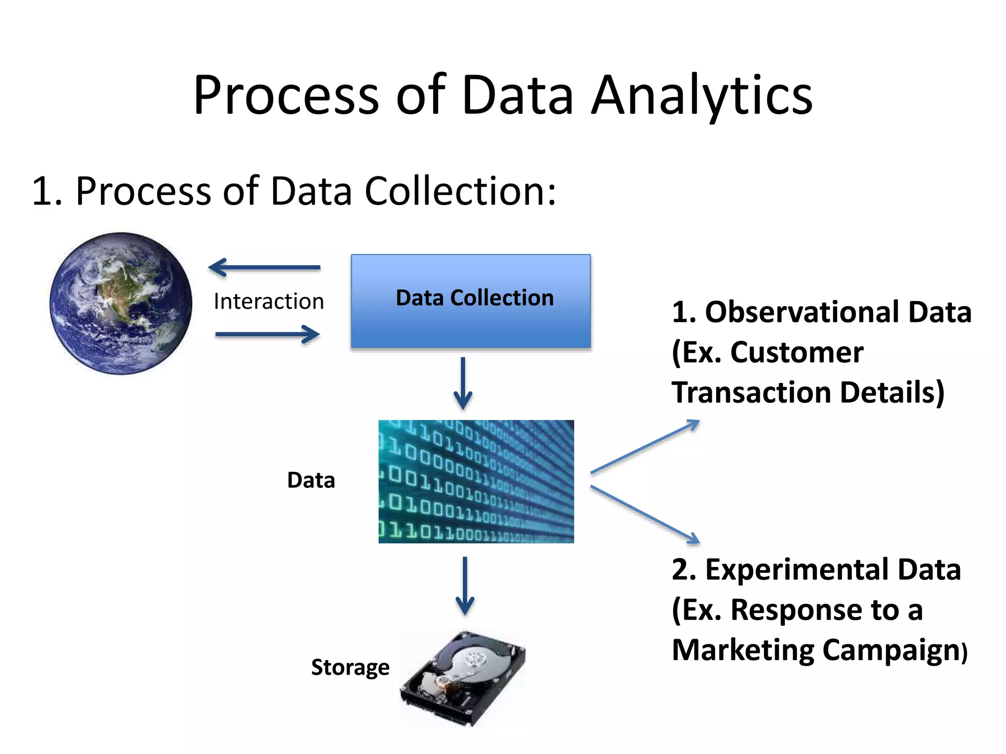
Process of DataAnalytics
Data CollectionInteraction
Data
2. Experimental Data
(Ex. Response to a
Marketing Campaign)
Storage
1. Process of Data Collection:
1. Observational Data
(Ex. Customer
Transaction Details)
75.
Process of DataAnalytics
2. Process of Data Analytics
Retrieval
Data pre-processing/cleaning
Data Analysis
[~80% of the time spent on making the data ready for the analysis]
76.
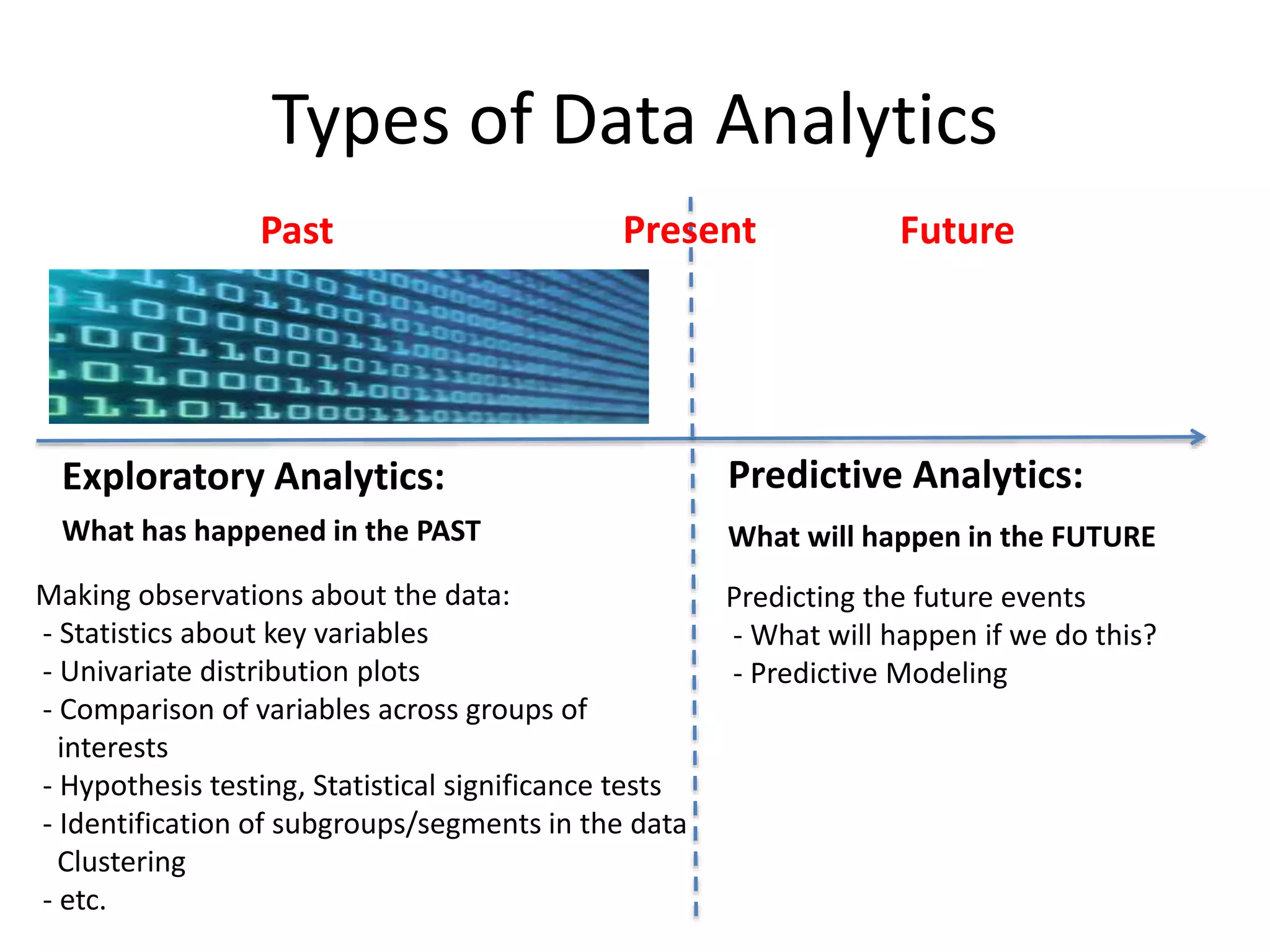
Types of DataAnalytics
Making observations about the data:
- Statistics about key variables
- Univariate distribution plots
- Comparison of variables across groups of
interests
- Hypothesis testing, Statistical significance tests
- Identification of subgroups/segments in the data
Clustering
- etc.
What has happened in the PAST What will happen in the FUTURE
Predicting the future events
- What will happen if we do this?
- Predictive Modeling
Exploratory Analytics: Predictive Analytics:
PresentPast Future
77.
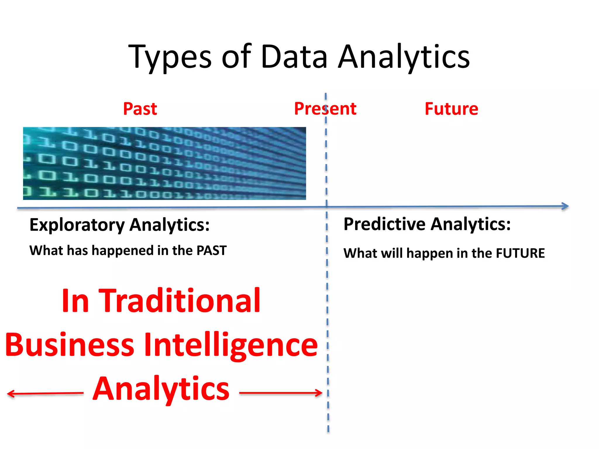
Types of DataAnalytics
What has happened in the PAST What will happen in the FUTURE
Exploratory Analytics: Predictive Analytics:
In Traditional
Business Intelligence
Analytics
PresentPast Future
78.
Types of DataAnalytics
What has happened in the PAST What will happen in the FUTURE
Exploratory Analytics: Predictive Analytics:
In Modern Data Science
PresentPast Future
79.
Predictive Analytics
Predicting whatwill happen in the FUTURE based on what has
happened in the PAST
Predictive Modeling
Statistical Modeling
Regression Analysis
Data Mining
Pattern Recognition
etc.
What has happened
in the past
What will happen
In the future
Machine Learning
Introduction to MachineLearning
“Field of study that gives computers the ability to learn without
being explicitly programmed”
82.
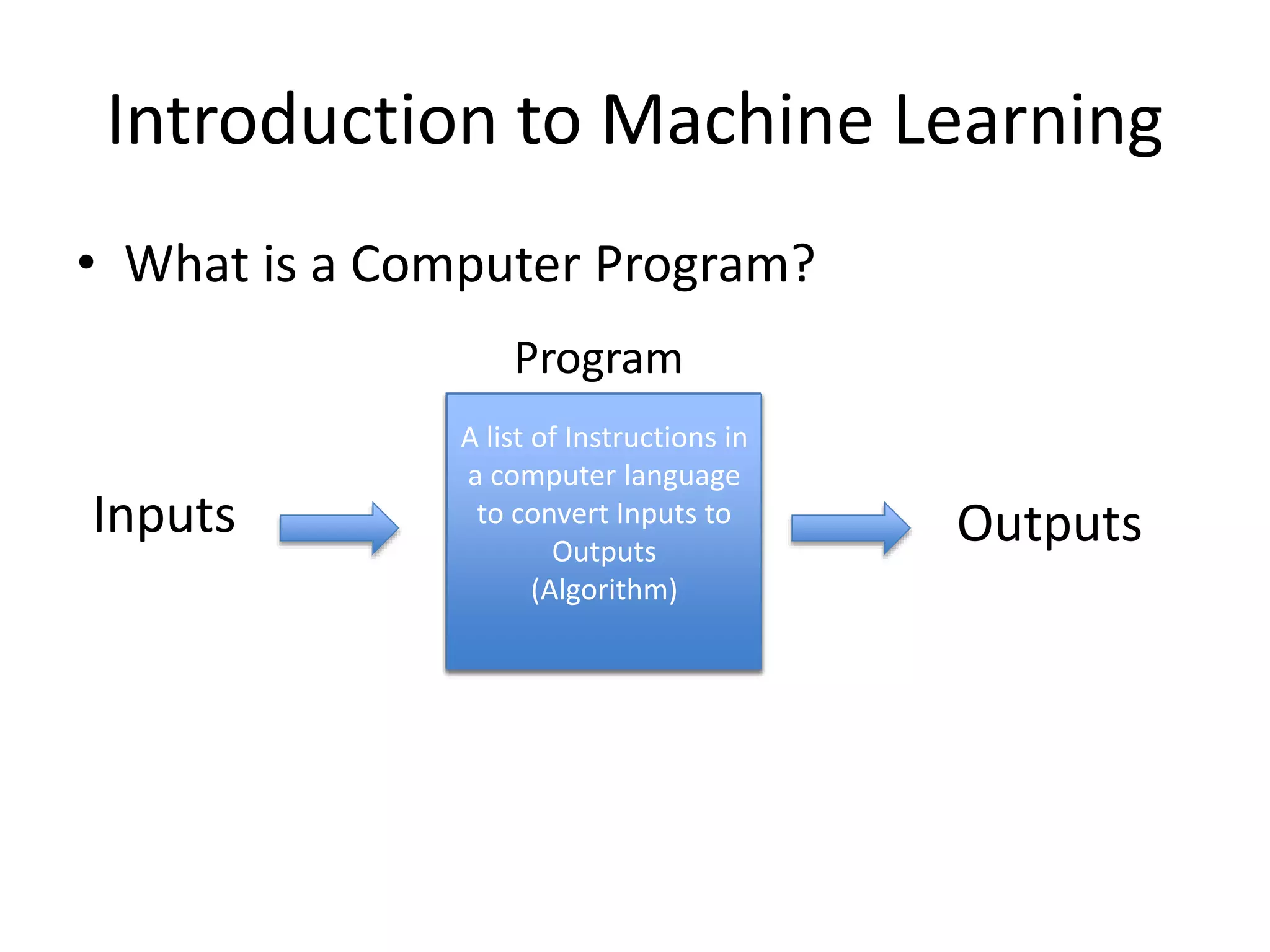
Introduction to MachineLearning
• What is a Computer Program?
List of Instructions in
a computer language
to map Inputs to
Outputs
(Algorithm)
Inputs Outputs
A list of Instructions in
a computer language
to convert Inputs to
Outputs
(Algorithm)
Program
83.
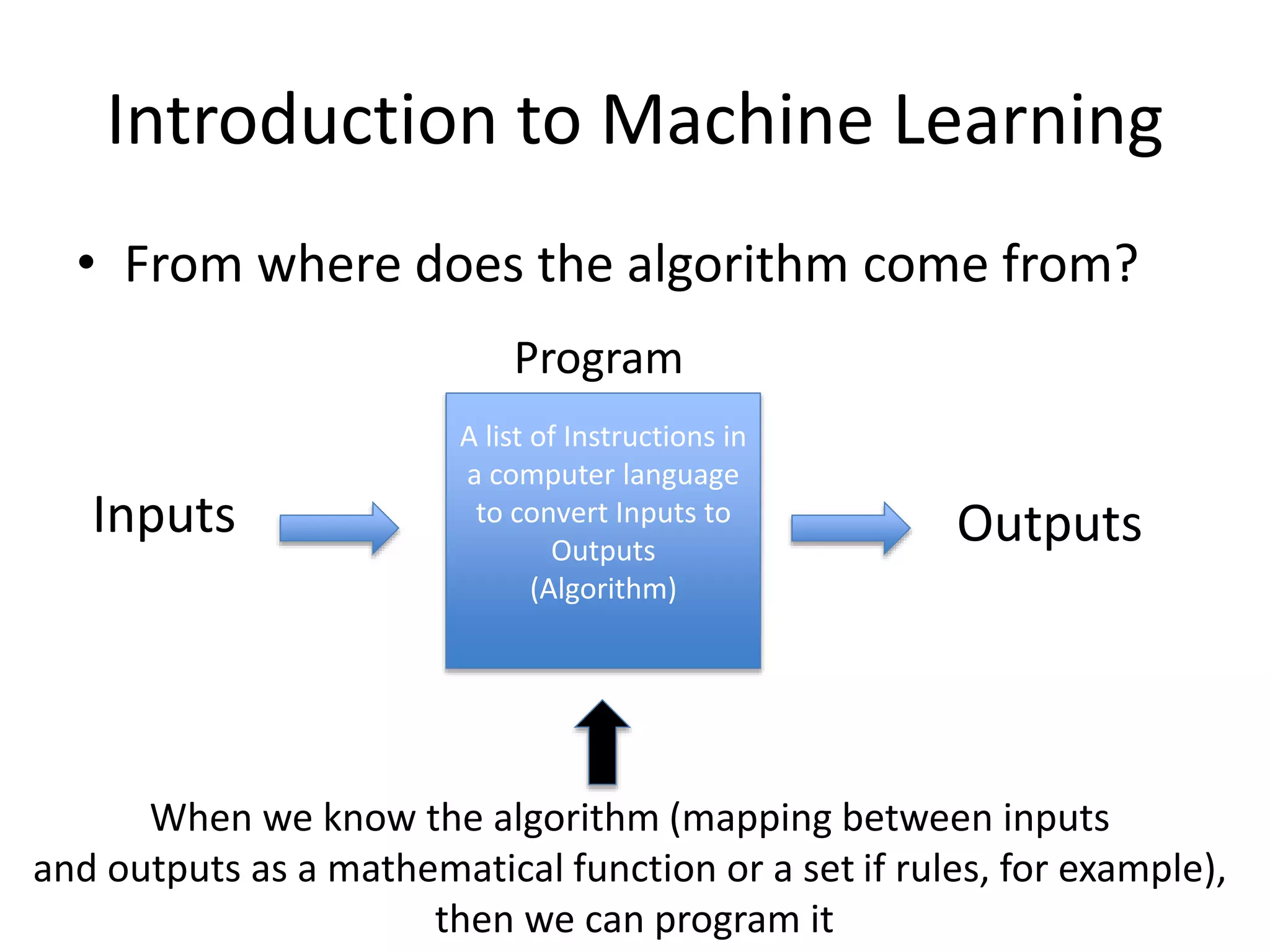
Introduction to MachineLearning
• From where does the algorithm come from?
A list of Instructions in
a computer language
to convert Inputs to
Outputs
(Algorithm)
Inputs Outputs
When we know the algorithm (mapping between inputs
and outputs as a mathematical function or a set if rules, for example),
then we can program it
Program
84.
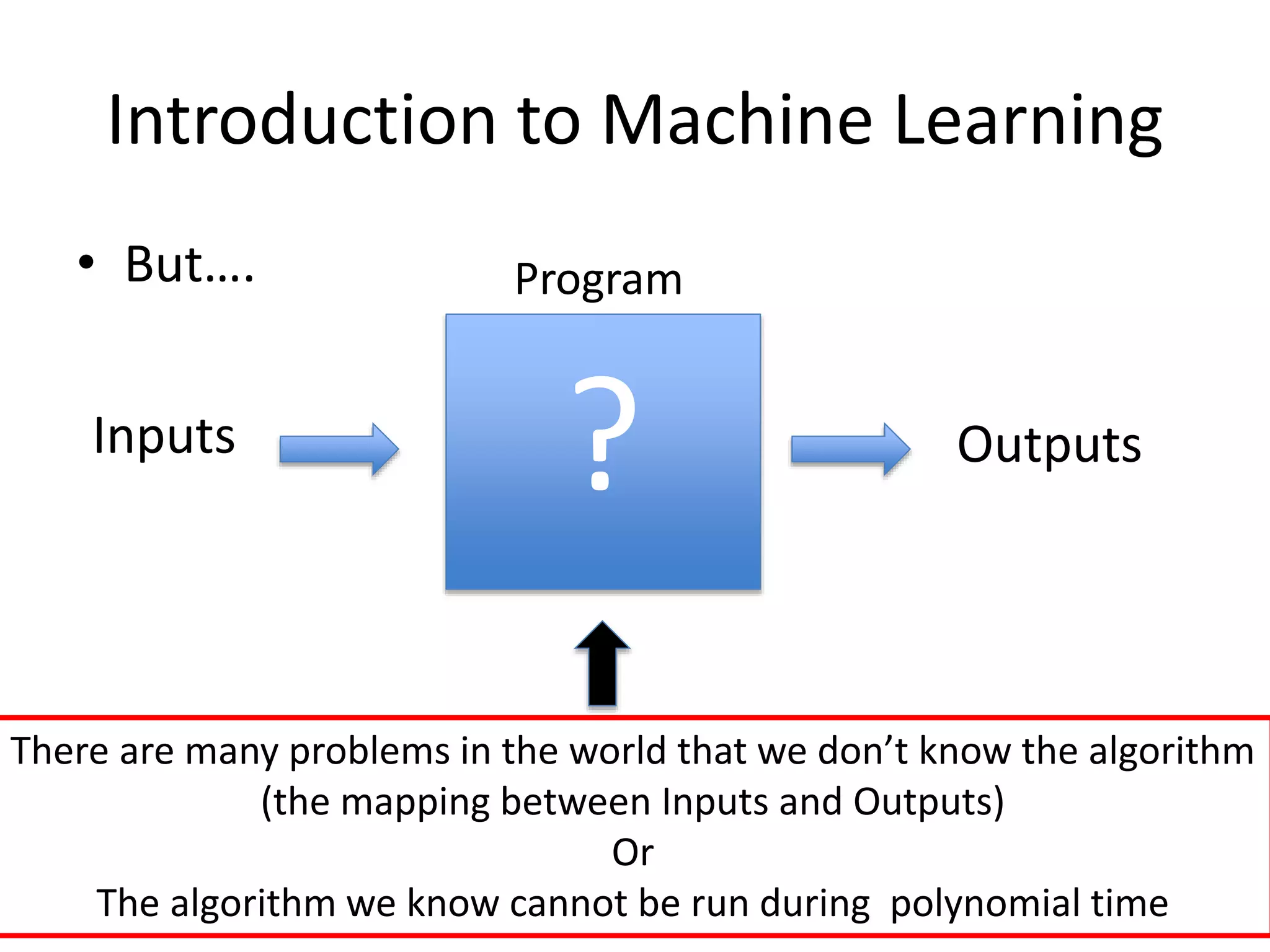
Introduction to MachineLearning
• But….
?Inputs Outputs
There are many problems in the world that we don’t know the algorithm
(the mapping between Inputs and Outputs)
Or
The algorithm we know cannot be run during polynomial time
Program
85.
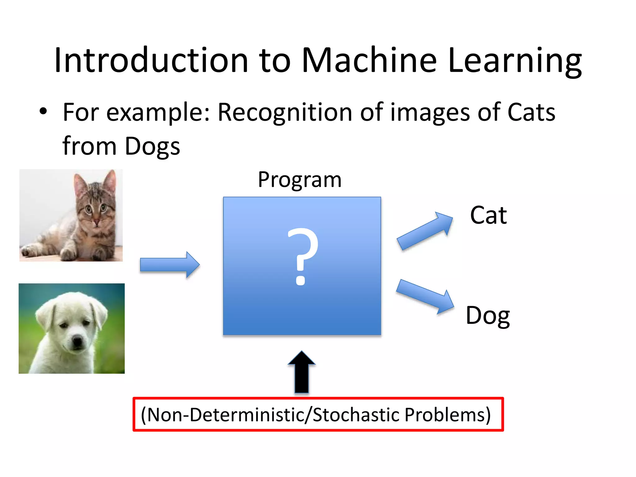
Introduction to MachineLearning
• For example: Recognition of images of Cats
from Dogs
? Dog
Program
(Non-Deterministic/Stochastic Problems)
Cat
86.
Introduction to MachineLearning
• For example: Predicting an email is good or
spam
?
Program
(Non-Deterministic/Stochastic Problems)
87.
Introduction to MachineLearning
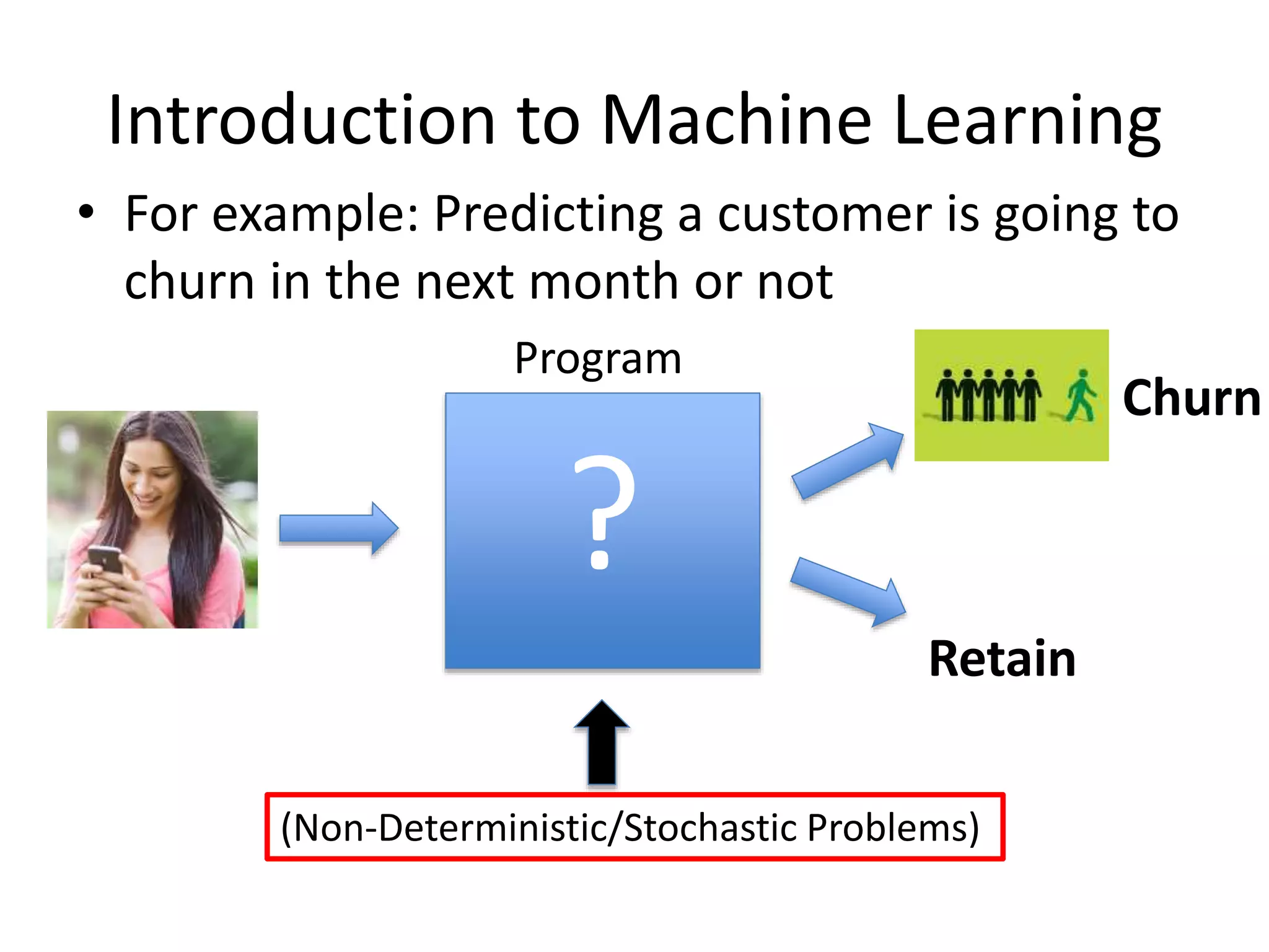
• For example: Predicting a customer is going to
churn in the next month or not
?
Program
Retain
Churn
(Non-Deterministic/Stochastic Problems)
88.
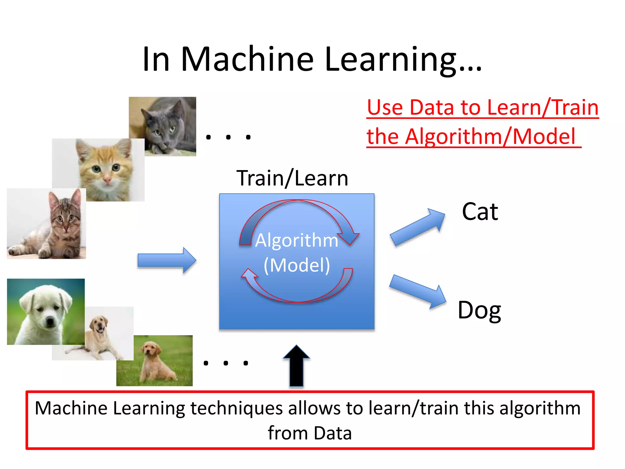
In Machine Learning…
Algorithm
(Model)
MachineLearning techniques allows to learn/train this algorithm
from Data
. . .
. . .
Train/Learn
Use Data to Learn/Train
the Algorithm/Model
Dog
Cat
89.
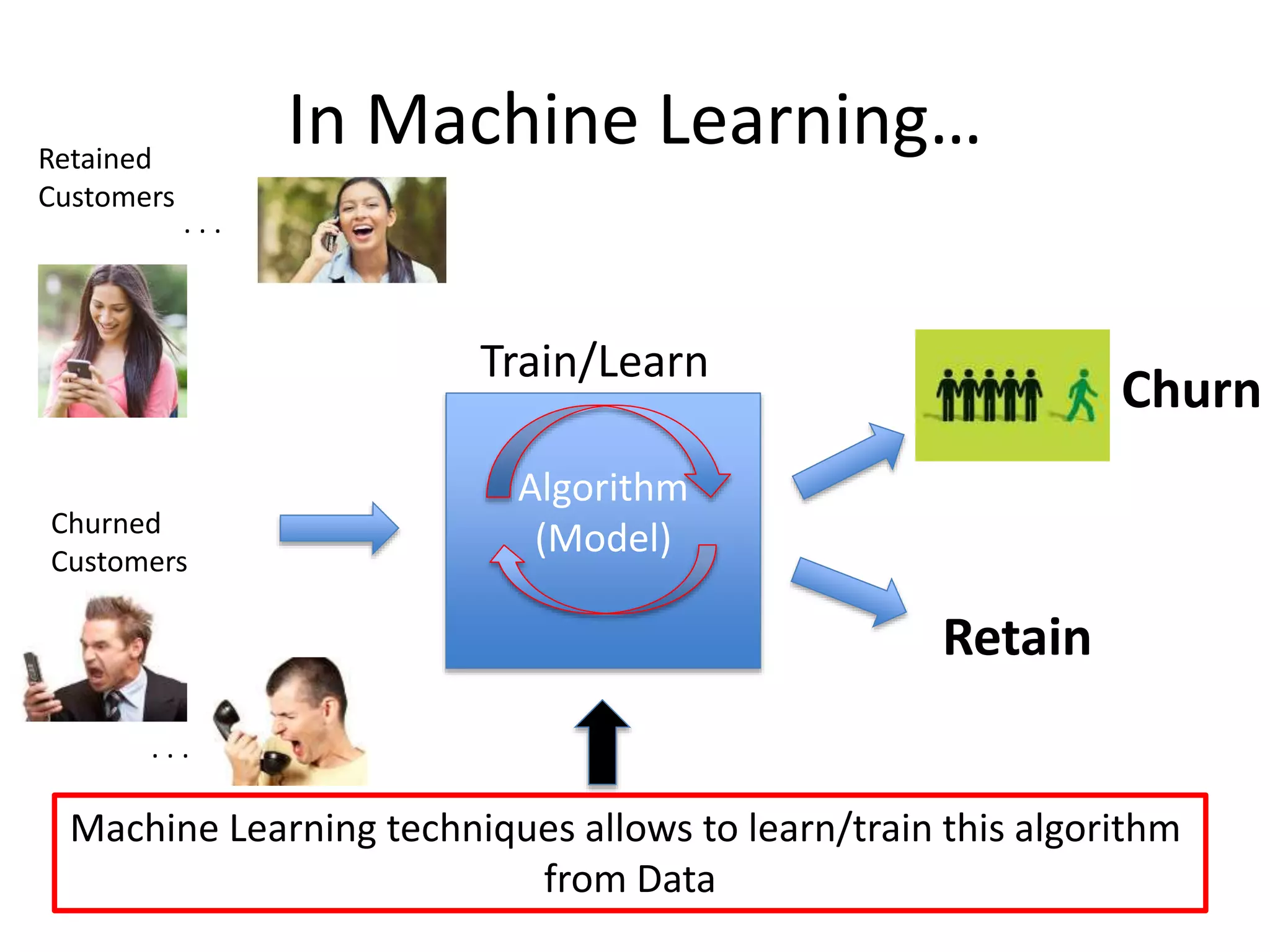
In Machine Learning…
Algorithm
(Model)
MachineLearning techniques allows to learn/train this algorithm
from Data
Train/Learn
. . .
. . .
Retained
Customers
Churned
Customers
Churn
Retain
90.
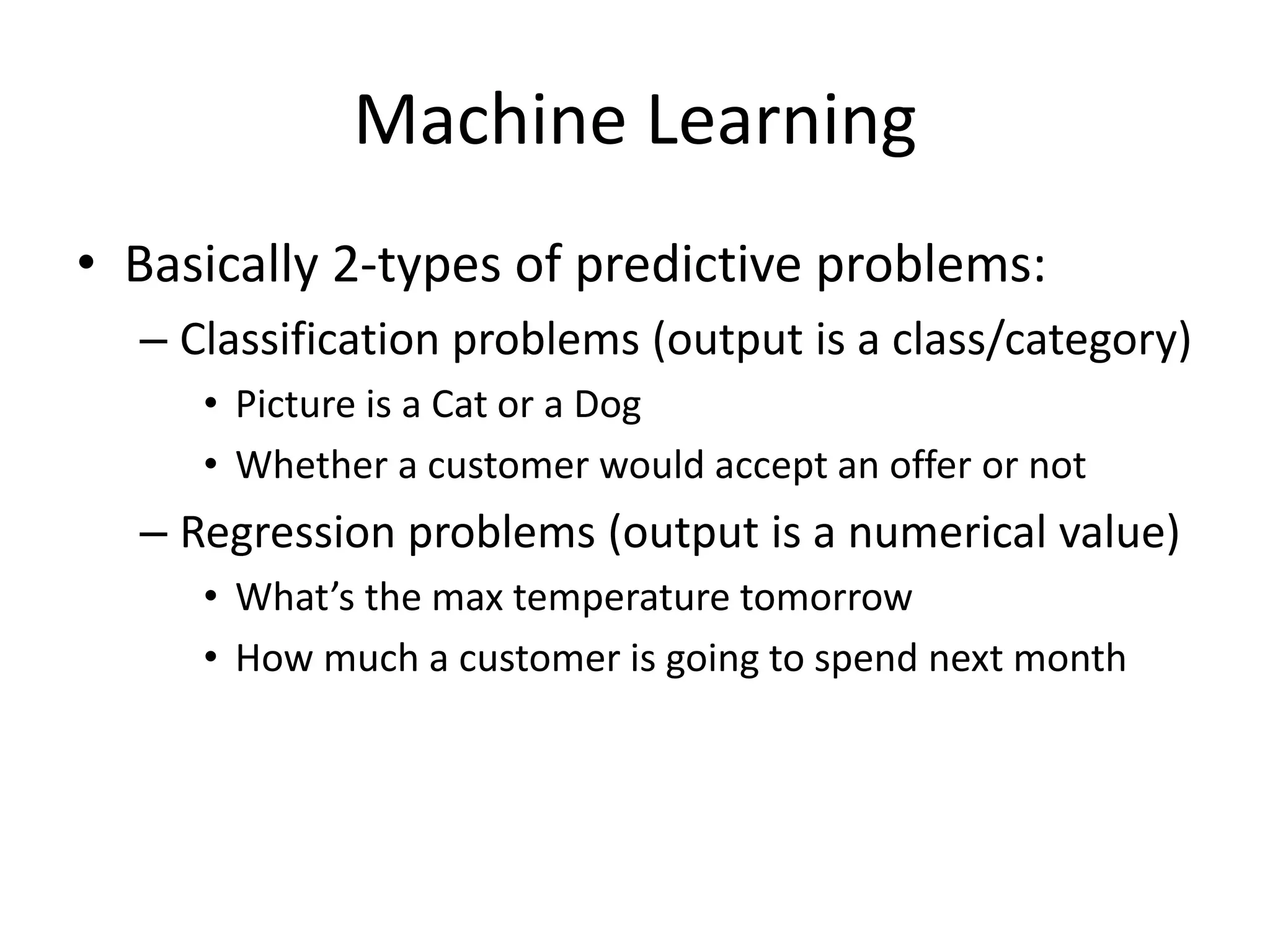
• Basically 2-typesof predictive problems:
– Classification problems (output is a class/category)
• Picture is a Cat or a Dog
• Whether a customer would accept an offer or not
– Regression problems (output is a numerical value)
• What’s the max temperature tomorrow
• How much a customer is going to spend next month
Machine Learning
91.
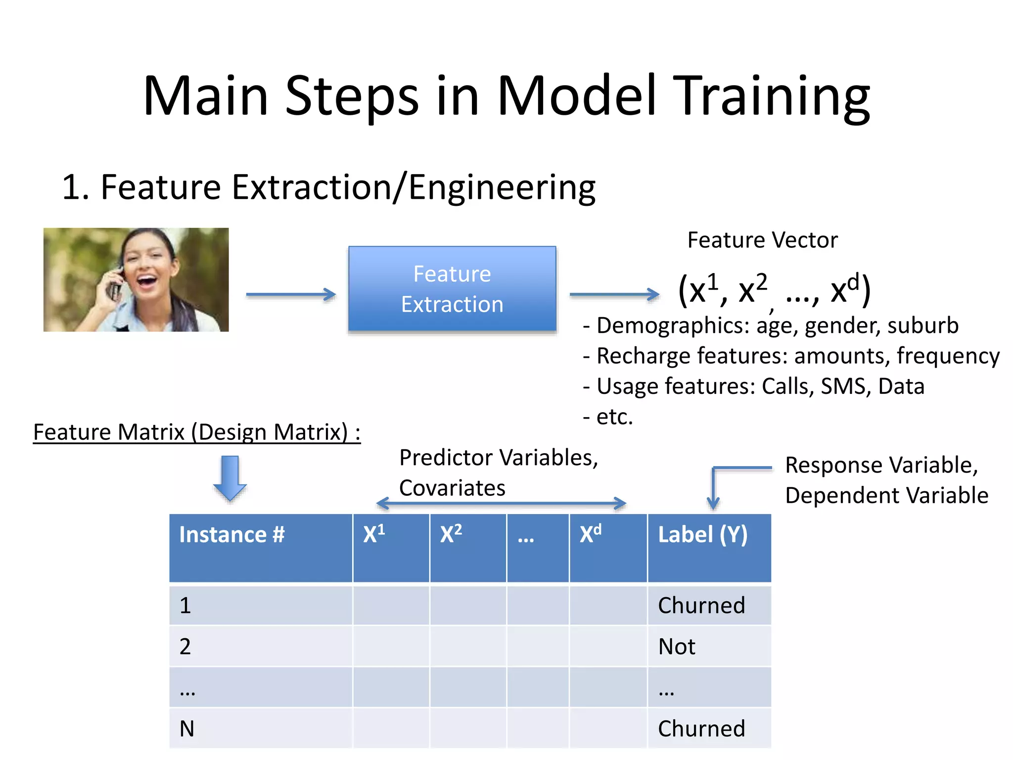
Main Steps inModel Training
Feature
Extraction (x1, x2
, …, xd)
Feature Vector
1. Feature Extraction/Engineering
Feature Matrix (Design Matrix) :
Instance # X1 X2 … Xd Label (Y)
1 Churned
2 Not
… …
N Churned
- Demographics: age, gender, suburb
- Recharge features: amounts, frequency
- Usage features: Calls, SMS, Data
- etc.
Predictor Variables,
Covariates
Response Variable,
Dependent Variable
92.
Main Steps inModel Training
2. Feature Pre-processing
• Convert categorical features into numerical ones
• Missing value imputation
• Outlier removal
• Normalization (bringing all features into the
same scale)
• Handle class imbalance
Instance # X1 X2 … Xd Label (Y)
1 Churned
2 Not
… …
N Churned
93.
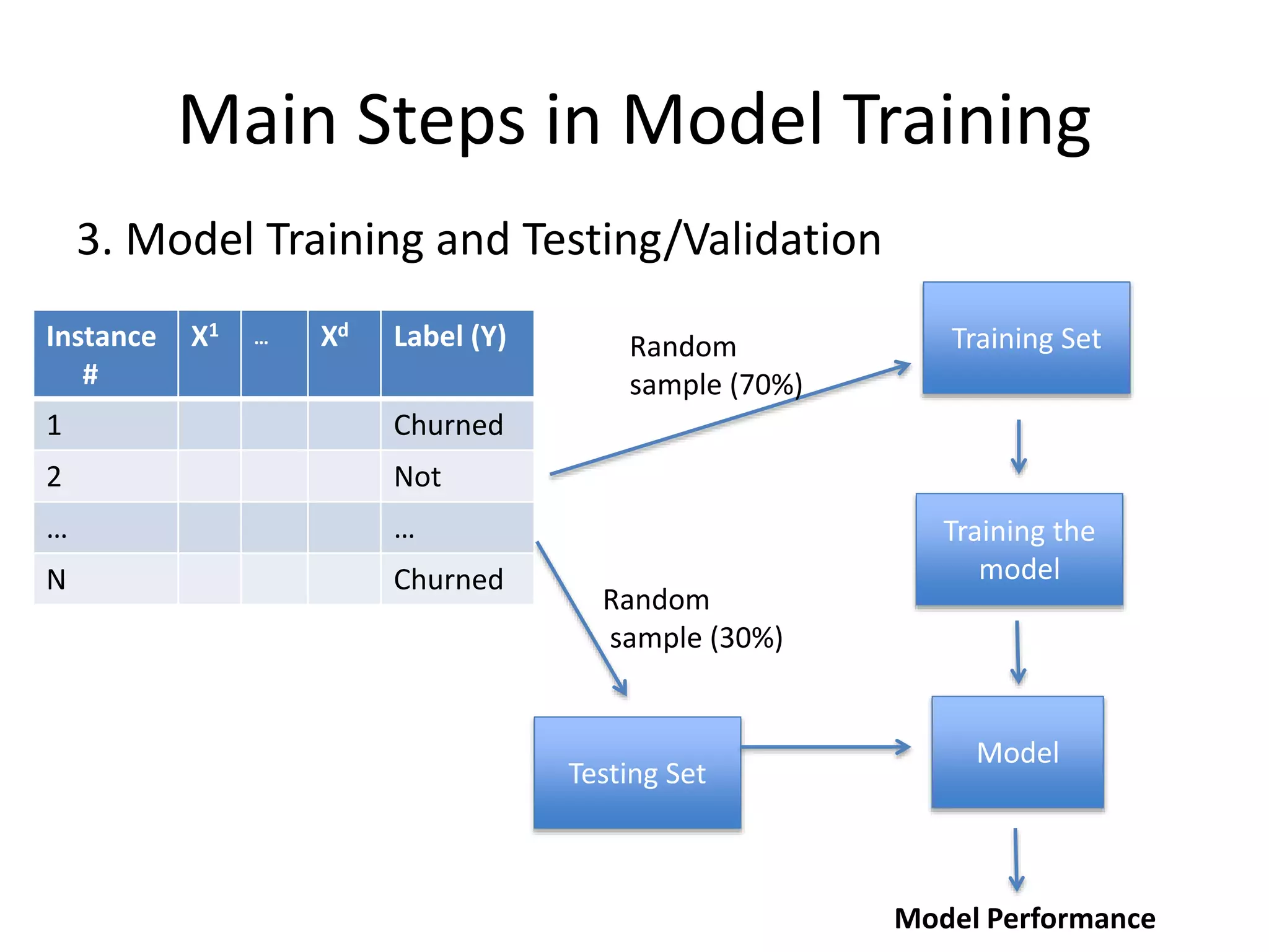
3. Model Trainingand Testing/Validation
Main Steps in Model Training
Training SetRandom
sample (70%)
Training the
model
Model
Testing Set
Random
sample (30%)
Model Performance
Instance
#
X1 … Xd Label (Y)
1 Churned
2 Not
… …
N Churned
94.
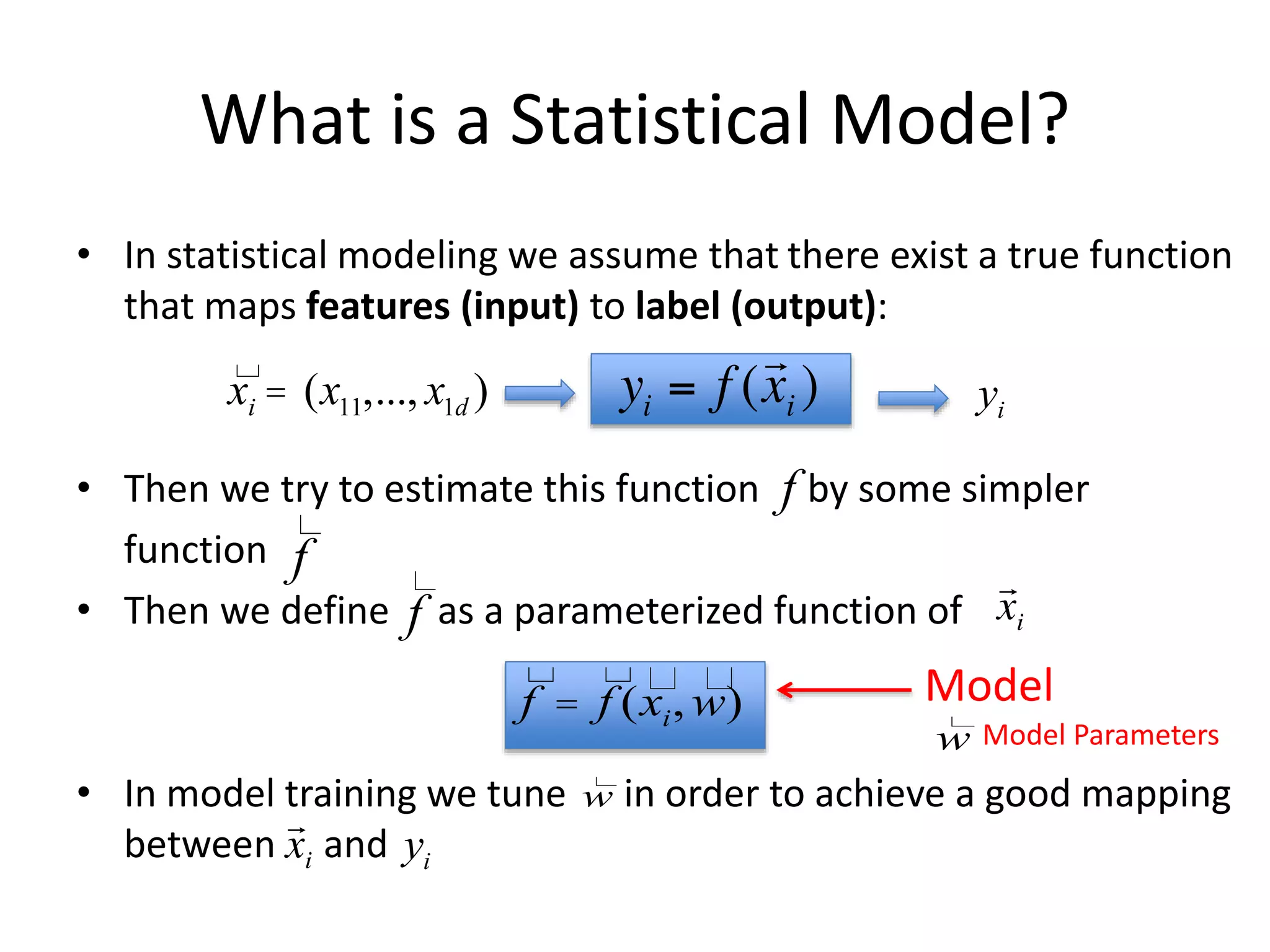
What is aStatistical Model?
• In statistical modeling we assume that there exist a true function
that maps features (input) to label (output):
• Then we try to estimate this function by some simpler
function
• Then we define as a parameterized function of
f
f
f = f (xi, w)
f
xi = (x11,..., x1d ) yi
95.
What is aStatistical Model?
• In statistical modeling we assume that there exist a true function
that maps features (input) to label (output):
• Then we try to estimate this function by some simpler
function
• Then we define as a parameterized function of
• In model training we tune in order to achieve a good mapping
between and
f
f
f = f (xi, w)
f
xi = (x11,..., x1d ) yi
Model
w Model Parameters
w
yi
96.
How do wetune W?
• Model: , where is the estimated value
of under the model:
• Loss Function:
– difference between actual label and the predicted label
• In Model Training:
ˆyi = ˆf (xi,w)
loss_ fn = L(yi, ˆyi ) = L(yi, ˆf (xi,w))
w*
= arg_min
w
[loss_ fn]= arg_min
w
[L(yi, f (xi,w))]
ˆyi
yi
97.
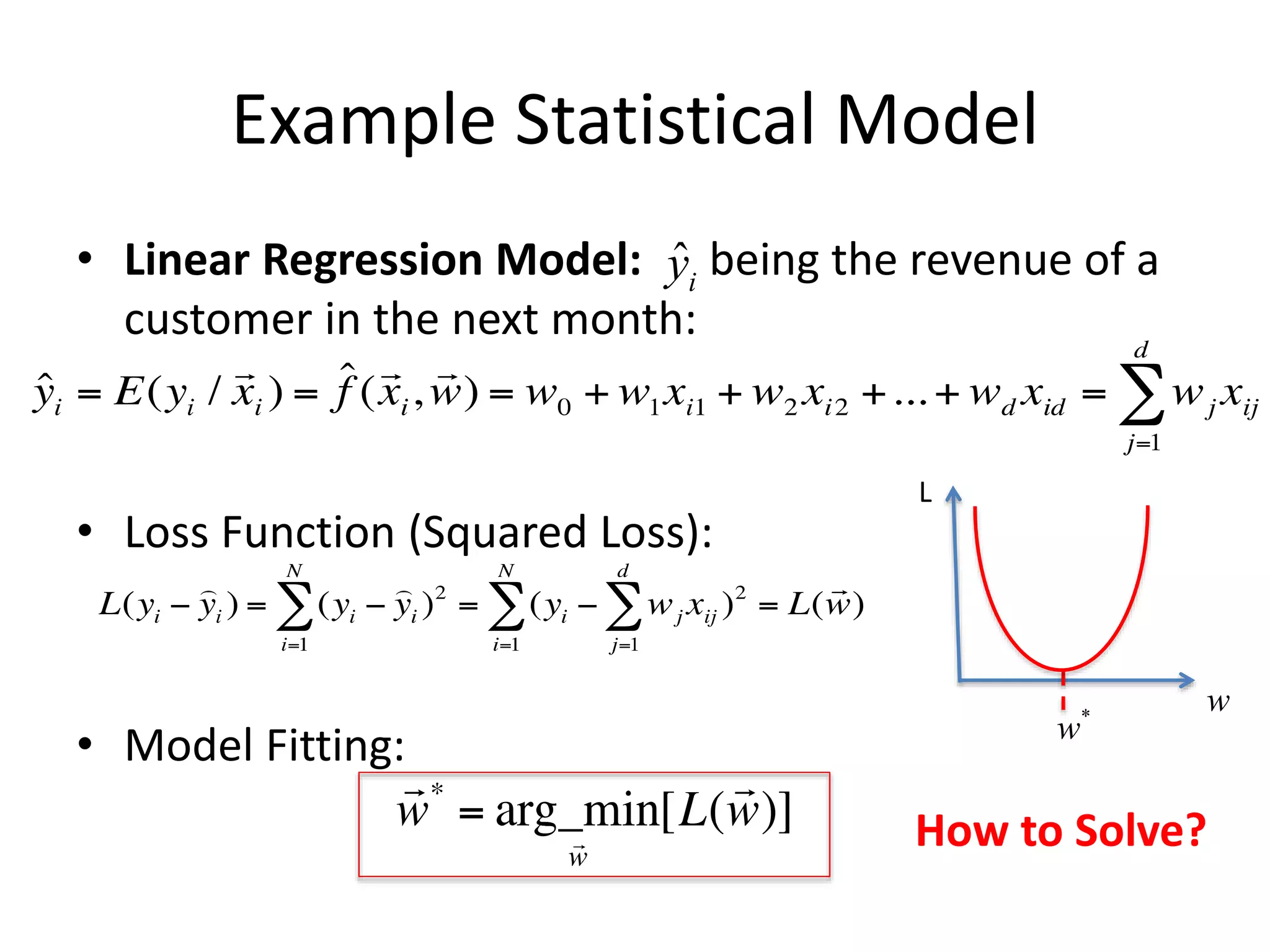
Example Statistical Model
•Linear Regression Model: being the revenue of a
customer in the next month:
• Loss Function (Squared Loss):
• Model Fitting:
L
w
w*
ˆyi
98.
Example Statistical Model
•Linear Regression Model: being the revenue of a
customer in the next month:
• Loss Function (Squared Loss):
• Model Fitting:
L
w
w*
ˆyi
How to Solve?
99.
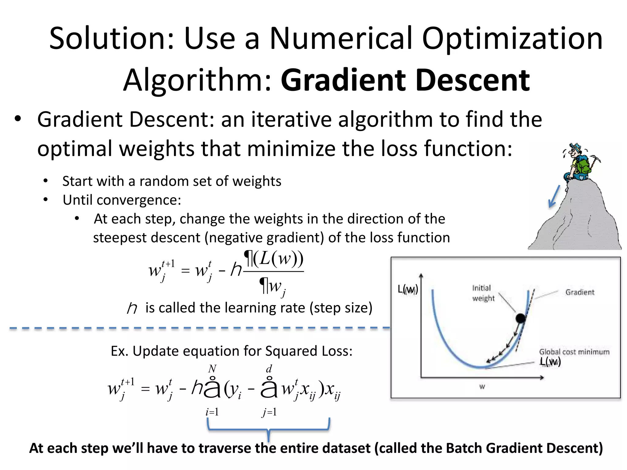
Solution: Use aNumerical Optimization
Algorithm: Gradient Descent
• Gradient Descent: an iterative algorithm to find the
optimal weights that minimize the loss function:
• Start with a random set of weights
• Until convergence:
• At each step, change the weights in the direction of the
steepest descent (negative gradient) of the loss function
wj
t+1
= wj
t
-h
¶(L(w))
¶wj
wj
t+1
= wj
t
-h (
i=1
N
å yi - wj
t
xij )xij
j=1
d
å
Ex. Update equation for Squared Loss:
h is called the learning rate (step size)
At each step we’ll have to traverse the entire dataset (called the Batch Gradient Descent)
L(w)
L(w)
100.
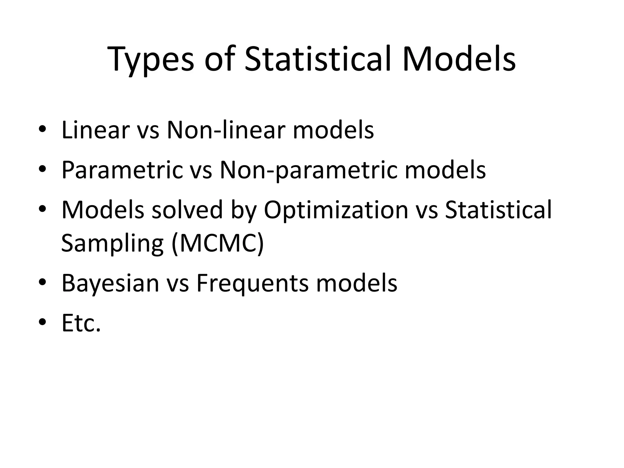
• Linear vsNon-linear models
• Parametric vs Non-parametric models
• Models solved by Optimization vs Statistical
Sampling (MCMC)
• Bayesian vs Frequents models
• Etc.
Types of Statistical Models
101.
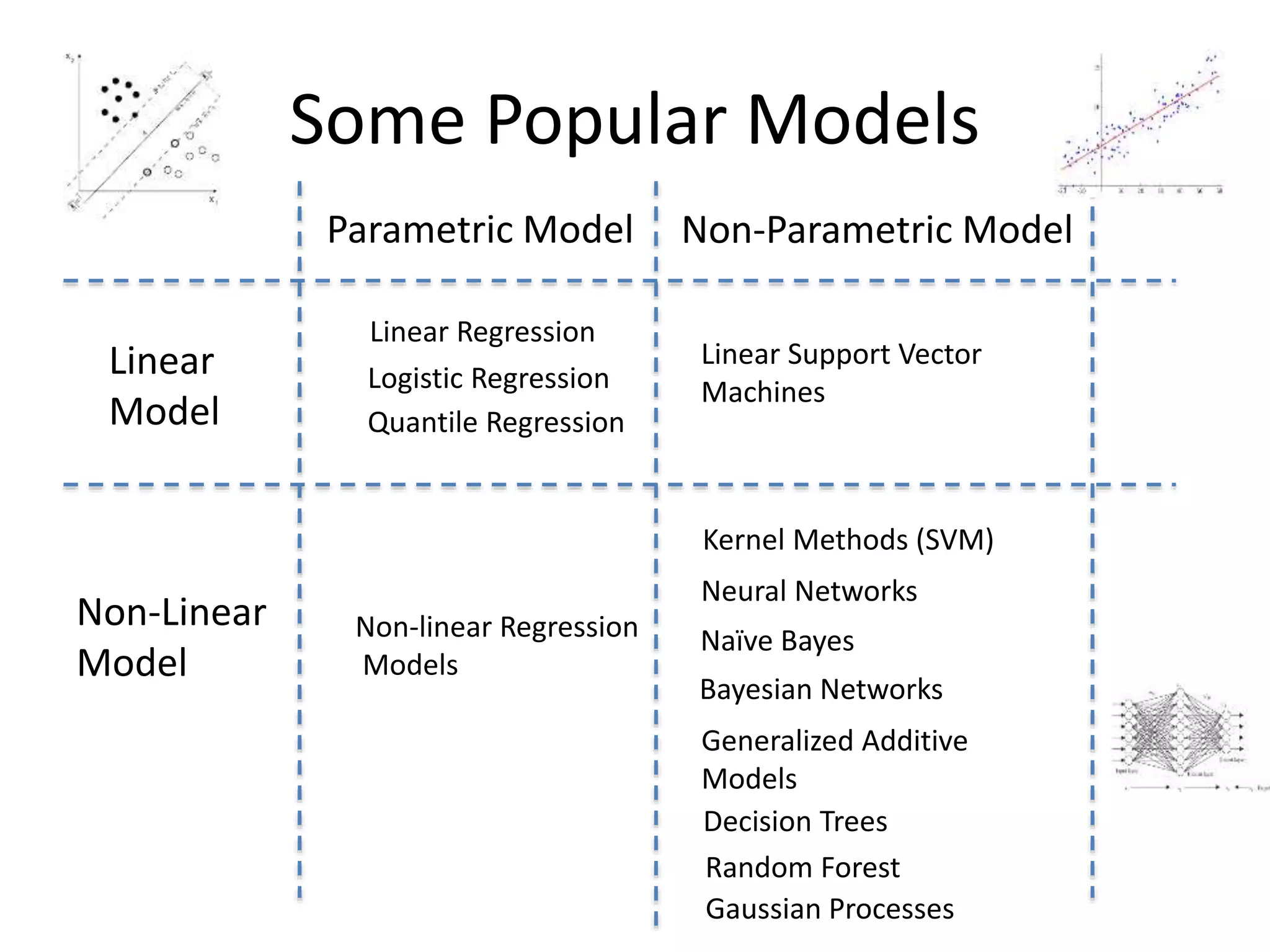
Some Popular Models
Linear
Model
Non-Linear
Model
ParametricModel Non-Parametric Model
Linear Regression
Logistic Regression
Non-linear Regression
Models
Linear Support Vector
Machines
Generalized Additive
Models
Decision Trees
Kernel Methods (SVM)
Bayesian Networks
Neural Networks
Random Forest
Quantile Regression
Naïve Bayes
Gaussian Processes
Model Underfitting vsOverfitting
• Underfitting (High Bias) – model is under-trained:
– Low performance of both training and testing datasets
• Overfitting (High Variance) – model is over-trained:
– High performance on the training dataset, but poor performance on
the testing dataset.
– Low generalization power
– Model is fitted to Noise rather than to Signal in the dataset
104.
Model Overfitting
Common reasons:
1.Over-specifying the model (higher model complexity),
more features in the model than necessary (called curse
of dimensionality)
Solution: Feature selection/Regularization
105.
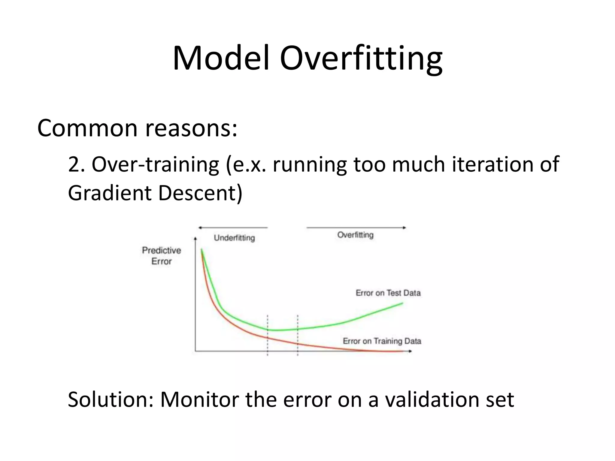
Model Overfitting
Common reasons:
2.Over-training (e.x. running too much iteration of
Gradient Descent)
Solution: Monitor the error on a validation set
106.
Some Techniques toImprove the
Model Performance
• Non-linear models/Non-linear features
• Hyper parameter tuning via cross validation
• Ensemble models
• Etc.
107.
Model Diagnostics
• Sanitychecking whether there is nothing
wrong with the model
• Test the assumption of the Data lead to the
selection of the model type.
• Many different diagnostics based on
regression or classification problems
108.
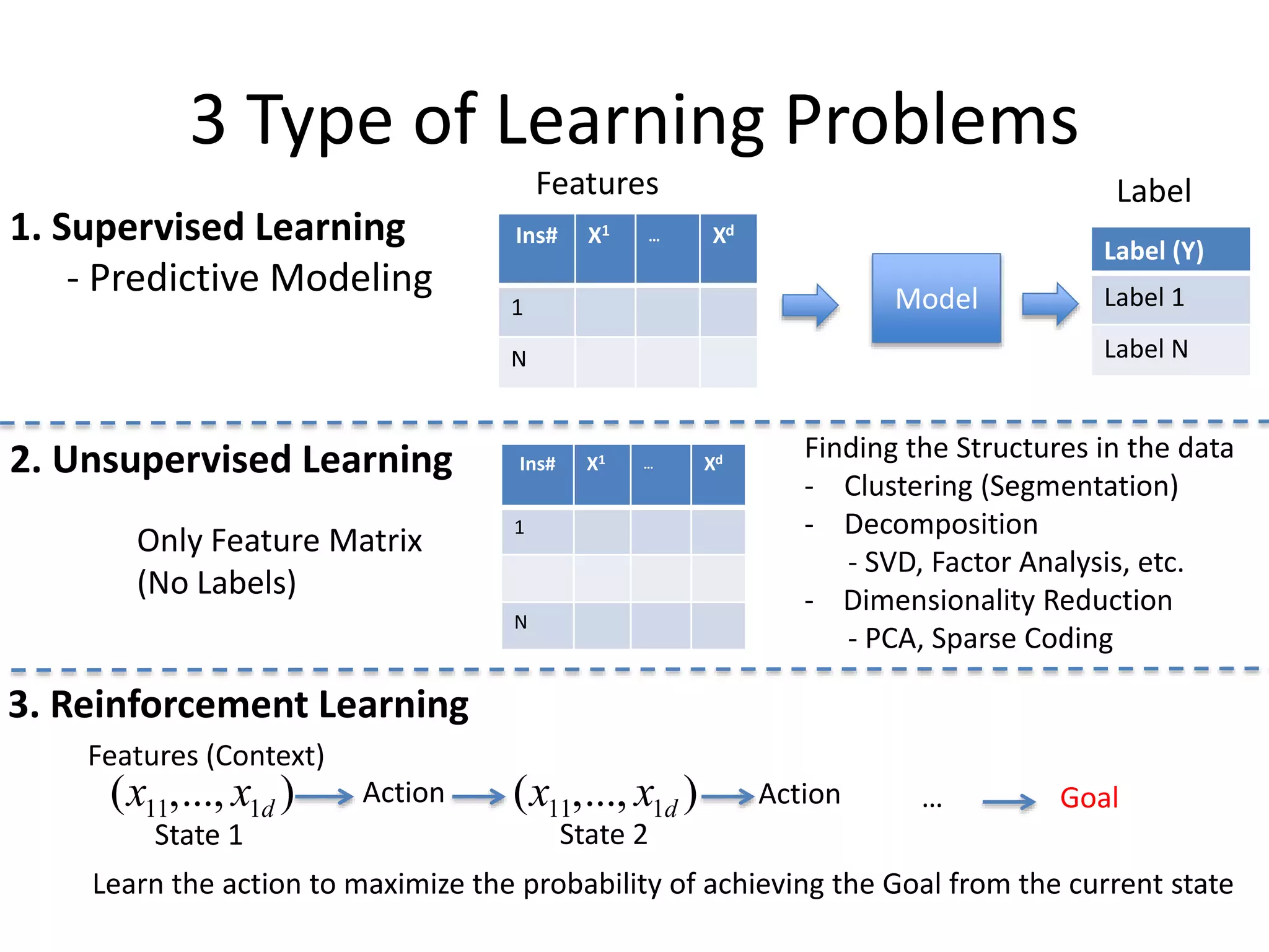
3 Type ofLearning Problems
Model
Features Label
1. Supervised Learning
- Predictive Modeling
Ins# X1 … Xd
1
N
Label (Y)
Label 1
Label N
2. Unsupervised Learning Ins# X1 … Xd
1
N
Finding the Structures in the data
- Clustering (Segmentation)
- Decomposition
- SVD, Factor Analysis, etc.
- Dimensionality Reduction
- PCA, Sparse Coding
3. Reinforcement Learning
Only Feature Matrix
(No Labels)
(x11,..., x1d )
Features (Context)
Action (x11,..., x1d )
State 1 State 2
Action … Goal
Learn the action to maximize the probability of achieving the Goal from the current state
109.
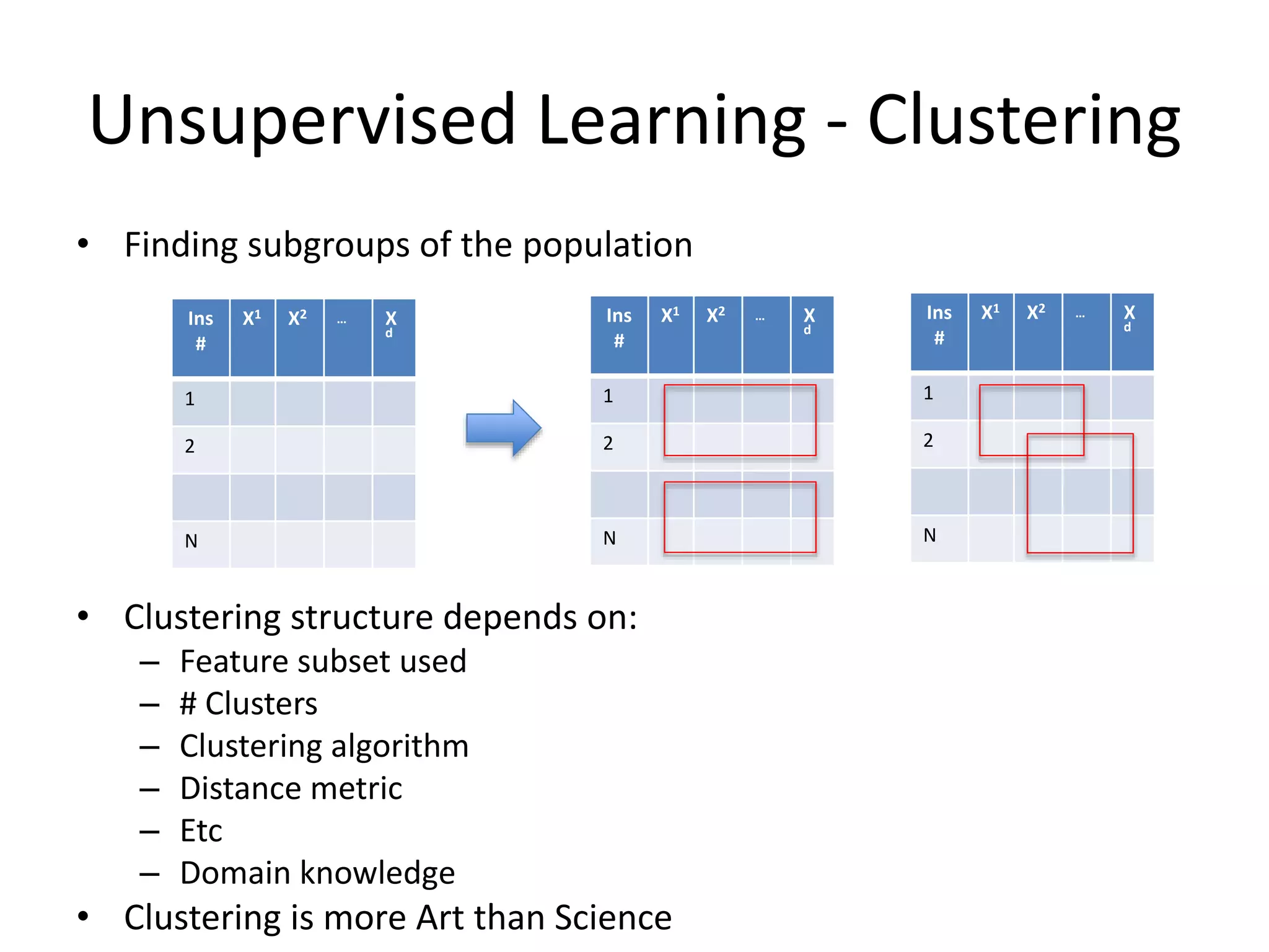
Unsupervised Learning -Clustering
• Finding subgroups of the population
• Clustering structure depends on:
– Feature subset used
– # Clusters
– Clustering algorithm
– Distance metric
– Etc
– Domain knowledge
• Clustering is more Art than Science
Ins
#
X1 X2 … X
d
1
2
N
Ins
#
X1 X2 … X
d
1
2
N
Ins
#
X1 X2 … X
d
1
2
N
110.
Data Visualization
• Alwaysvisualize your data!
• Powerful way of communication between
business and data science
• Exploratory analytics, model building stage,
model diagnostic, interpreting results, etc.
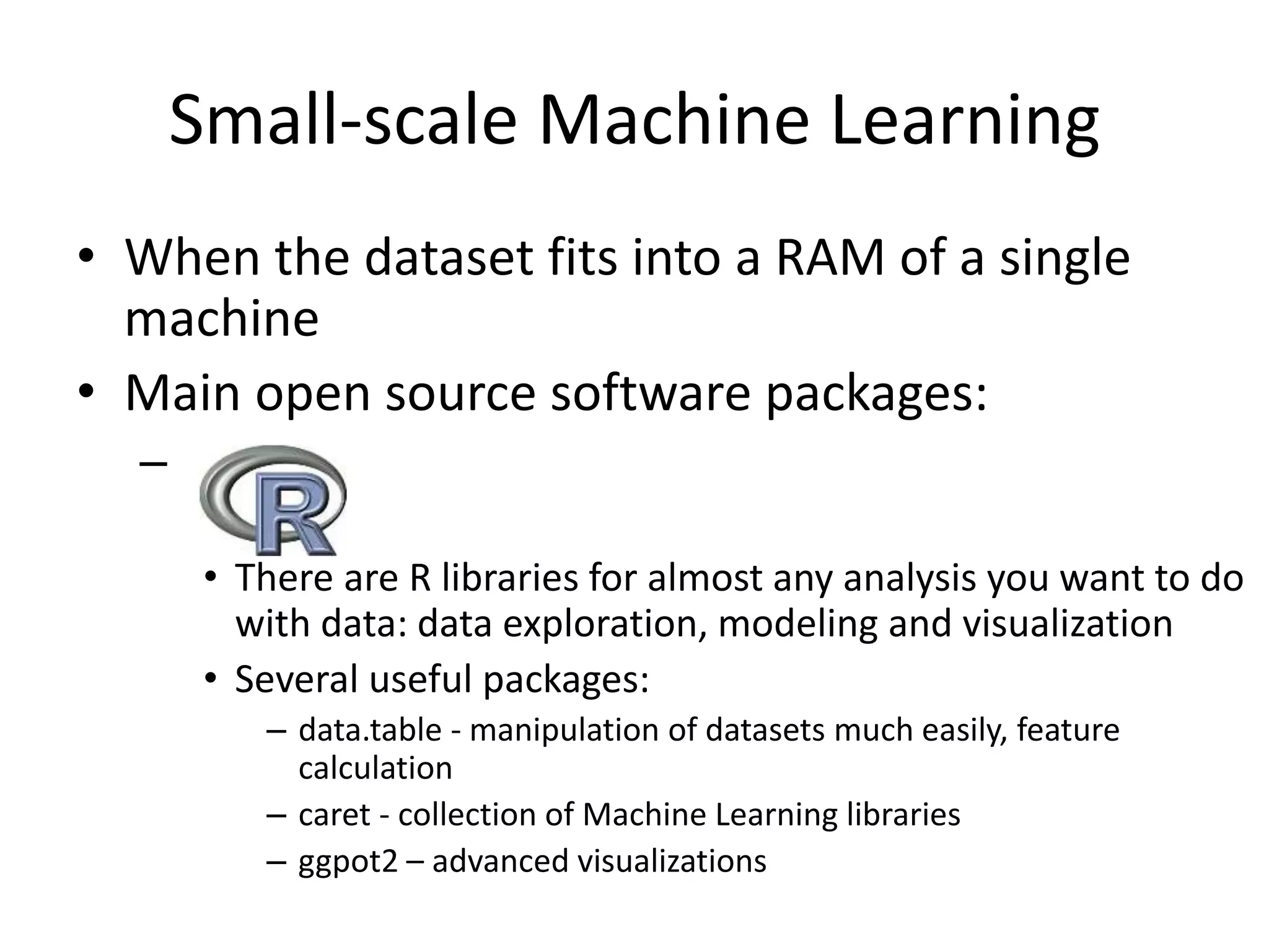
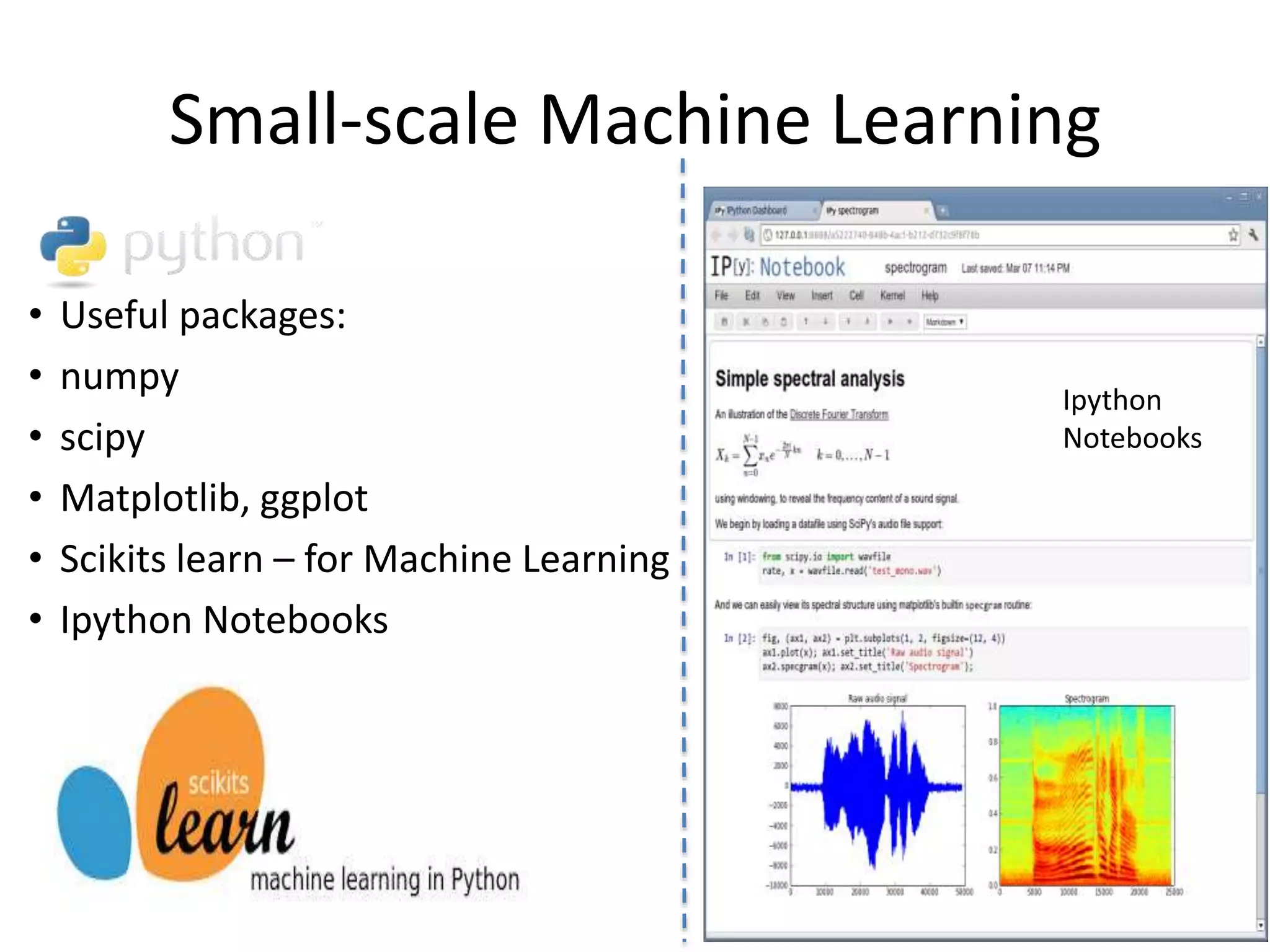
Small-scale Machine Learning
•When the dataset fits into a RAM of a single
machine
• Main open source software packages:
– .
• There are R libraries for almost any analysis you want to do
with data: data exploration, modeling and visualization
• Several useful packages:
– data.table - manipulation of datasets much easily, feature
calculation
– caret - collection of Machine Learning libraries
– ggpot2 – advanced visualizations
Large-scale Machine Learning
•When there are millions or billions of instances
– Computational advertising
– Spam classification (Gmail has 900 Million users)
– Facebook 2.2 Billion users
– Customer analytics in Supermarkets, Telcos, Banks,
Insurance, Media etc, where Millions of users.
• When there are millions of features
• When the models needs to be updated more
frequently (every hour, etc.)
– Computational advertising, recommendation systems,
systematic trading, etc.
http://www.businessinsider.com.au/facebook-inc-has-22-billion-users-2014-7
http://expandedramblings.com/index.php/gmail-statistics/
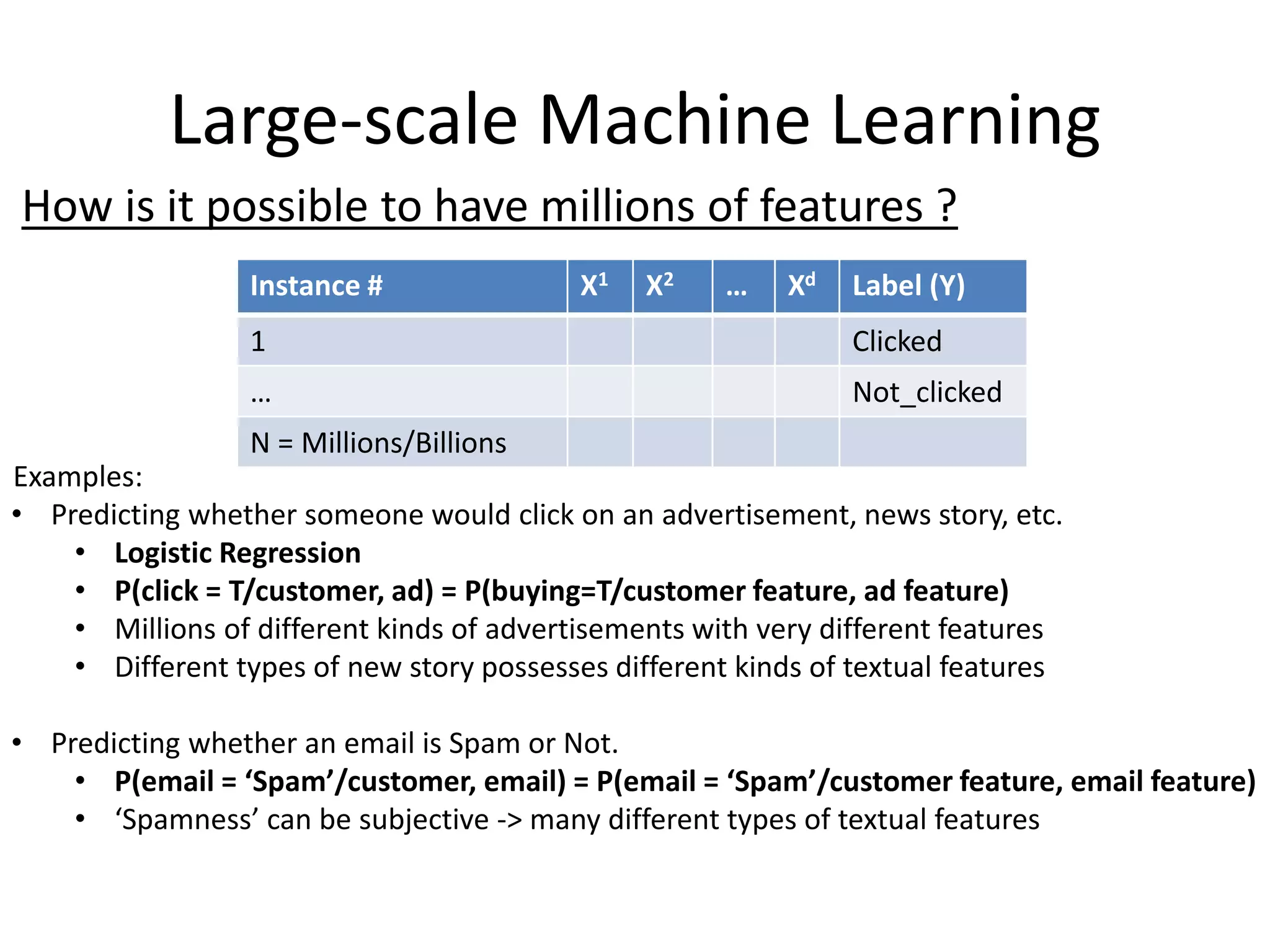
117.
Large-scale Machine Learning
Instance# X1 X2 … Xd Label (Y)
1 Clicked
… Not_clicked
N = Millions/Billions
Examples:
• Predicting whether someone would click on an advertisement, news story, etc.
• Logistic Regression
• P(click = T/customer, ad) = P(buying=T/customer feature, ad feature)
• Millions of different kinds of advertisements with very different features
• Different types of new story possesses different kinds of textual features
• Predicting whether an email is Spam or Not.
• P(email = ‘Spam’/customer, email) = P(email = ‘Spam’/customer feature, email feature)
• ‘Spamness’ can be subjective -> many different types of textual features
How is it possible to have millions of features ?
118.
Large-scale Machine Learning
Examples:
•Predicting whether a customer would buy a product or not in an online retailer like
Amazon, Alibaaba (millions of product), even a supermarkets, bookstore (100,000s products)
• P(buying = T/customer, product) = P(buying=T/customer feature, product feature)
How is it possible to have millions of features/parameters ?
…
119.
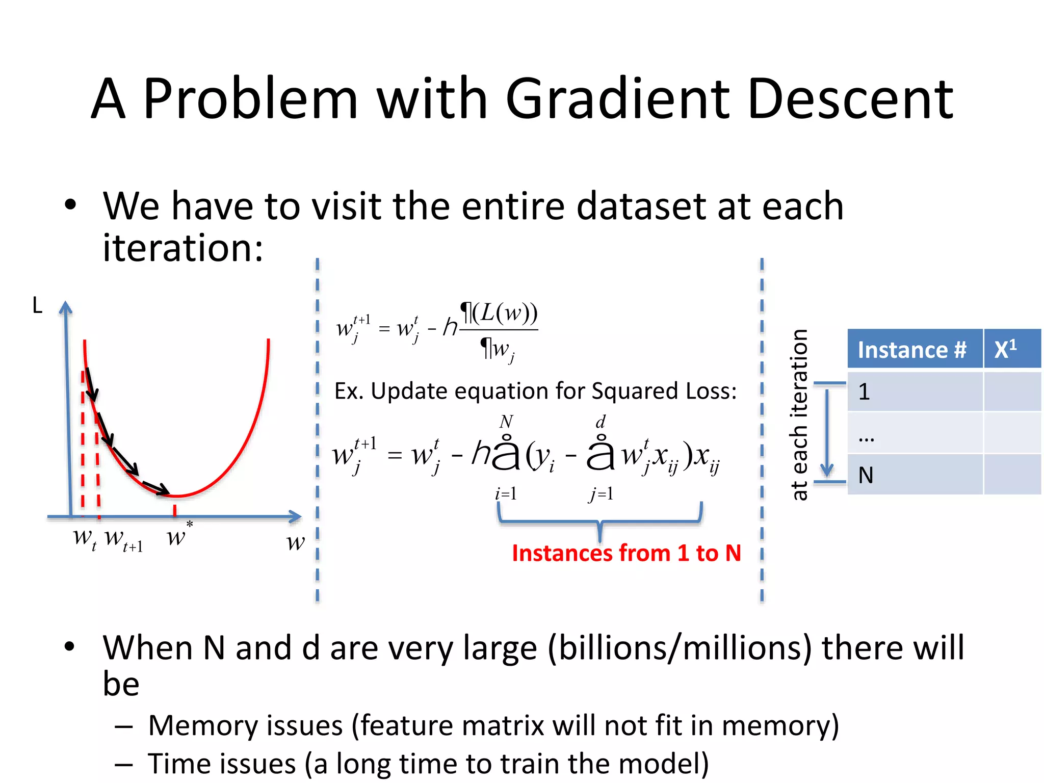
• We haveto visit the entire dataset at each
iteration:
• When N and d are very large (billions/millions) there will
be
– Memory issues (feature matrix will not fit in memory)
– Time issues (a long time to train the model)
A Problem with Gradient Descent
wj
t+1
= wj
t
-h
¶(L(w))
¶wj
wj
t+1
= wj
t
-h (
i=1
N
å yi - wj
t
xij )xij
j=1
d
å
Ex. Update equation for Squared Loss:
L
ww*
wt wt+1
Instances from 1 to N
Instance # X1
1
…
N
ateachiteration
120.
How to TrainLarge-scale Models?
1. Efficient single-machine Machine Learning
algorithms - (E.x. Improved Gradient
Descent)
2. Parallelization of Machine Learning algorithms
Stochastic Gradient Descent
•Stochastic Gradient Descent (Online Gradient
Descent)
L
ww*
wt wt+1
wj
t+1
= wj
t
-h (
i=1
N
å yi - wj
t
xij )xij
j=1
p
å
Batch Gradient Descent
(for Squared Loss):
Stochastic Gradient Descent:
At each iteration the weights are updated
w.r.t. a single training instance:
Until convergence repeat:
For each instance i
For each weight j
wj
t+1
= wj
t
-h(yi - wj
t
xij )xij
j=1
p
å
Until convergence repeat:
For each weight j
Instance # X1
1
2
…
N
ateachiteration
Instance # X1
1
2
…
N
Iter - 1
Instances from 1 to N
Iter - 2
Iter - N
123.
Massive-scale Machine Learningwith
Vowpal Wabbit (VW)
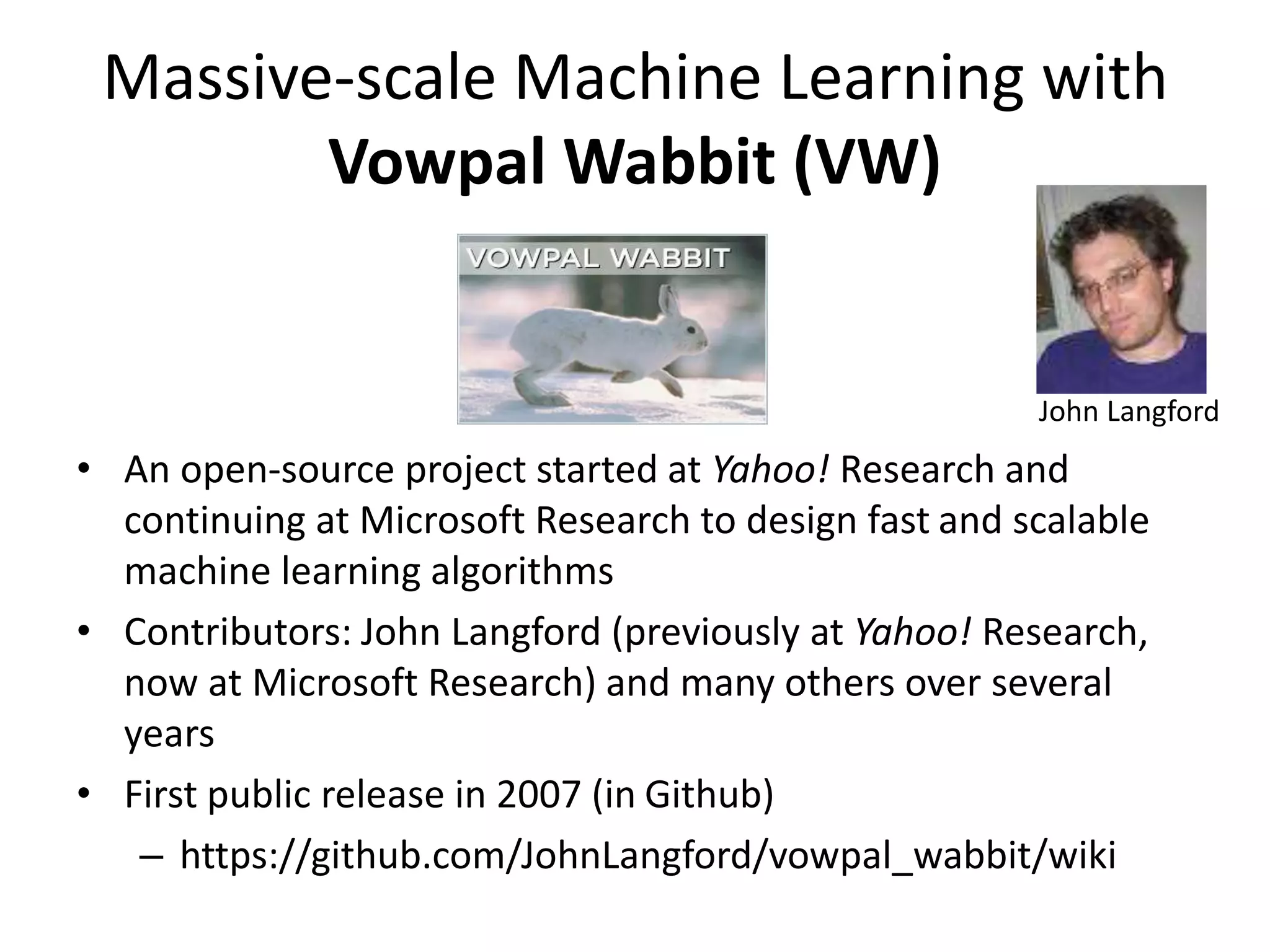
• An open-source project started at Yahoo! Research and
continuing at Microsoft Research to design fast and scalable
machine learning algorithms
• Contributors: John Langford (previously at Yahoo! Research,
now at Microsoft Research) and many others over several
years
• First public release in 2007 (in Github)
– https://github.com/JohnLangford/vowpal_wabbit/wiki
John Langford
124.
Massive-scale Machine Learningwith
Vowpal Wabbit (VW)
• VW allows you to train models with
millions/billions of training instances and
millions/billions of features in your laptop within
minutes!
• How can this be possible?
– Fast optimization algorithm
• Stochastic Gradient Descent with advanced tricks (coming
from cutting-edge large scale Machine Learning research)
– Efficient memory management
– Highly optimized C++ code
125.
Massive-scale Machine Learningwith
Vowpal Wabbit (VW)
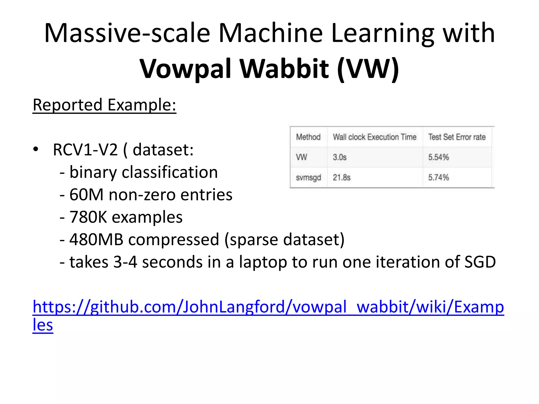
Reported Example:
• RCV1-V2 ( dataset:
- binary classification
- 60M non-zero entries
- 780K examples
- 480MB compressed (sparse dataset)
- takes 3-4 seconds in a laptop to run one iteration of SGD
https://github.com/JohnLangford/vowpal_wabbit/wiki/Examp
les
126.
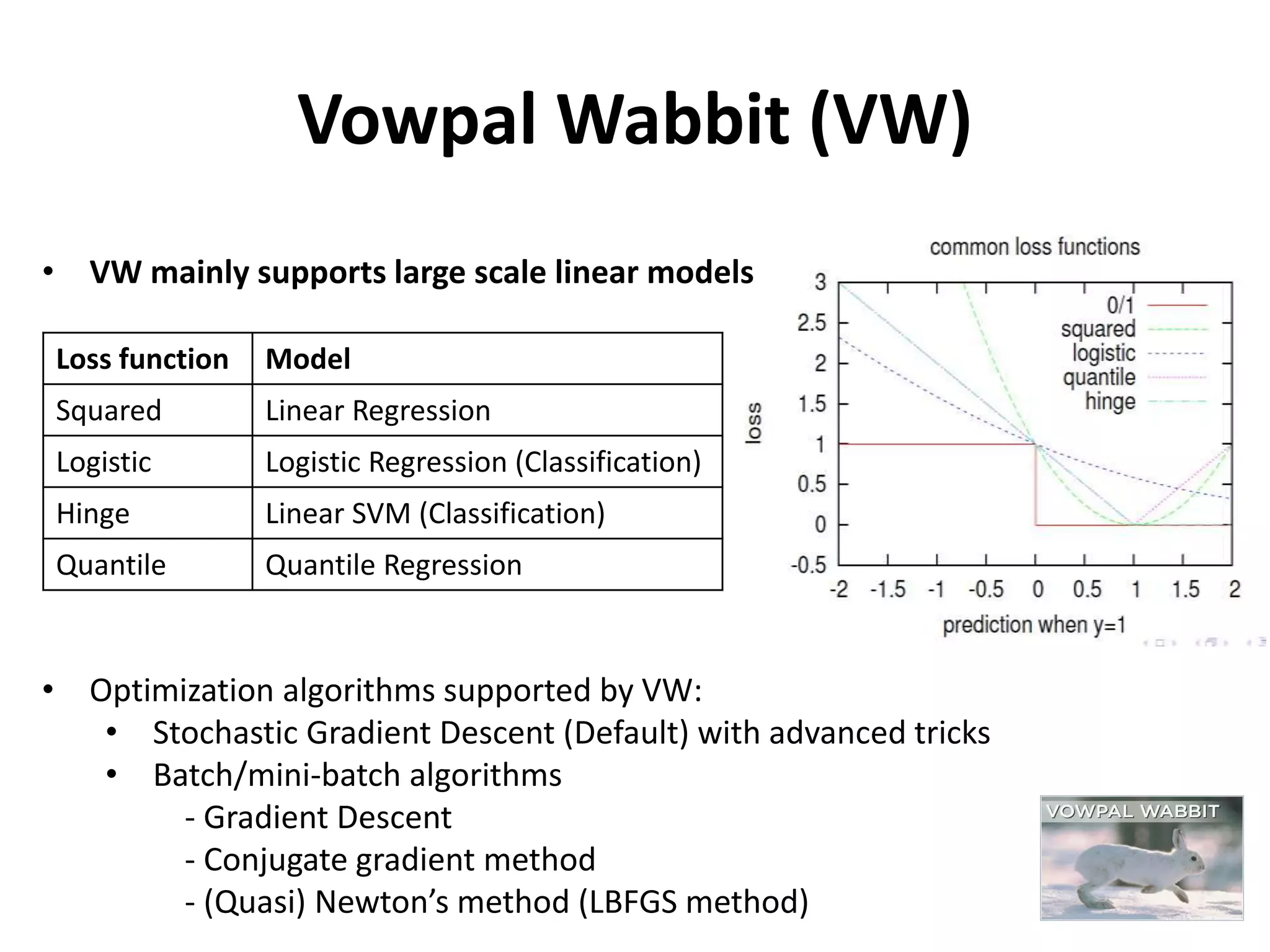
Vowpal Wabbit (VW)
Lossfunction Model
Squared Linear Regression
Logistic Logistic Regression (Classification)
Hinge Linear SVM (Classification)
Quantile Quantile Regression
• VW mainly supports large scale linear models
• Optimization algorithms supported by VW:
• Stochastic Gradient Descent (Default) with advanced tricks
• Batch/mini-batch algorithms
- Gradient Descent
- Conjugate gradient method
- (Quasi) Newton’s method (LBFGS method)
127.
Vowpal Wabbit (VW)
•Constant memory footprint
– VW only maintains the model parameter vector (weight vector) in the
memory and all the data is on the disk
– VW reads one training instance at a time into memory when calculating
the gradient – so you can have Billions of instances!
– For multiple passes over a dataset VW creates a binary cache version of
the input data file -> much faster read in from the disk
• Feature Hashing
– Feature names are hashed (32-bit murmurHash function) to
map into the locations of the weight vector in the memory
– Fast updates and efficient memory usage (no need to maintain a
feature dictionary)
– Default is 18 bit hash function [max is 32bits ~ 4 billion
features!]
Very Efficient Memory Management:
128.
Vowpal Wabbit (VW)
•Main input data format is text files or stdin
• Sparse representation of features:
[Label] [Importance weight] [id]|Namespace f_name1:val1 …|Namespace f_name1:val1 … |…
129.
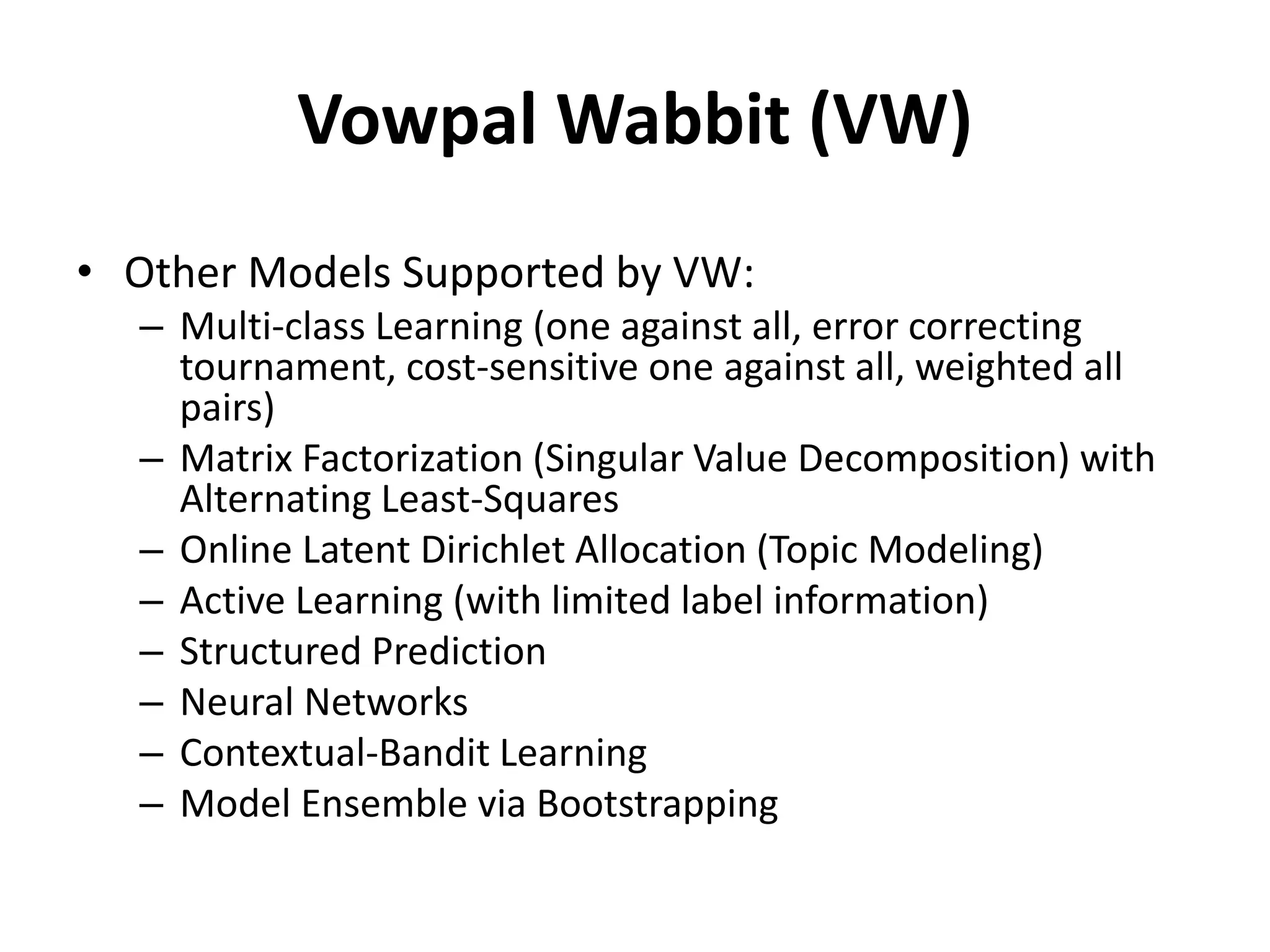
Vowpal Wabbit (VW)
•Other Models Supported by VW:
– Multi-class Learning (one against all, error correcting
tournament, cost-sensitive one against all, weighted all
pairs)
– Matrix Factorization (Singular Value Decomposition) with
Alternating Least-Squares
– Online Latent Dirichlet Allocation (Topic Modeling)
– Active Learning (with limited label information)
– Structured Prediction
– Neural Networks
– Contextual-Bandit Learning
– Model Ensemble via Bootstrapping
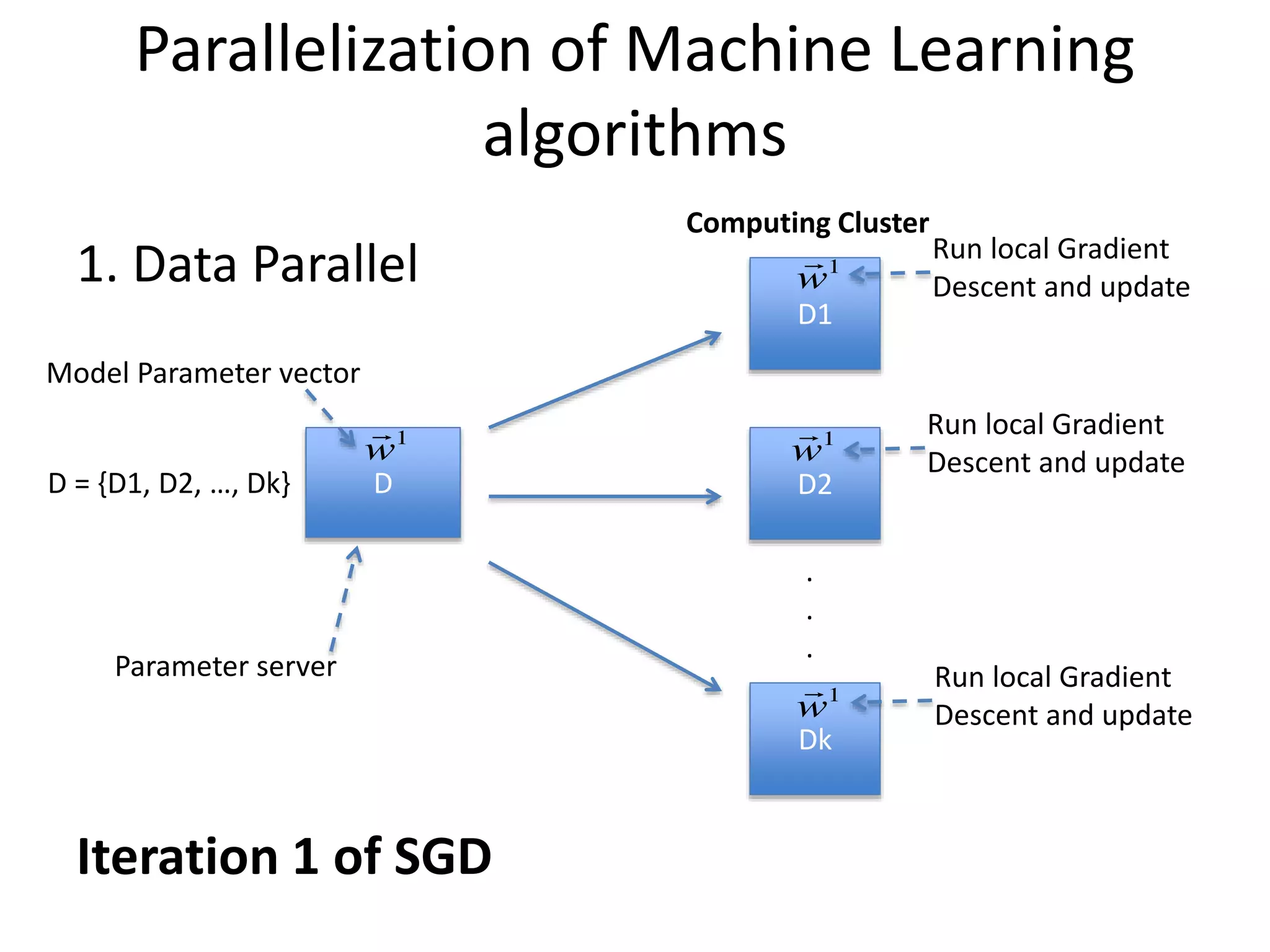
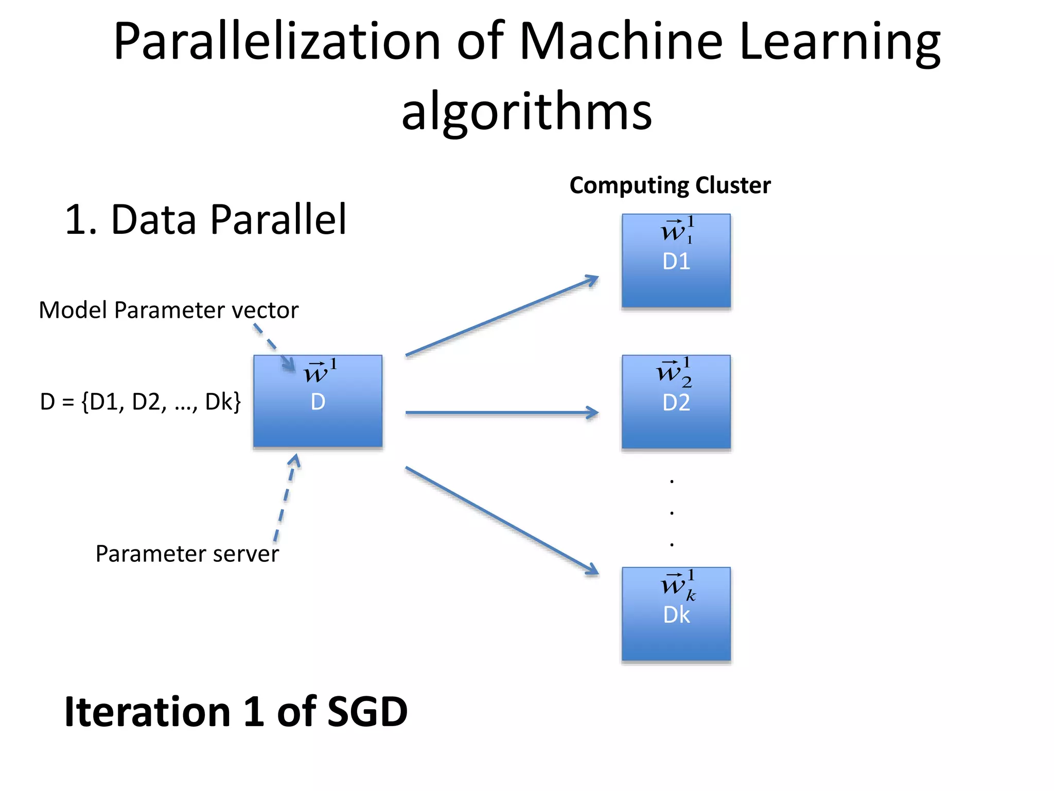
Parallelization of MachineLearning
algorithms
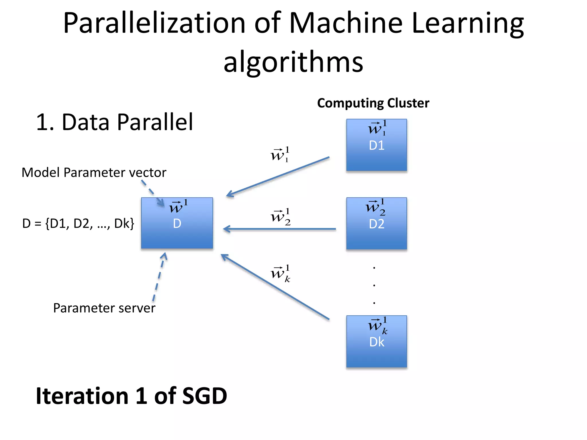
1. Data Parallel
D
D1
D2
Dk
.
.
.
D = {D1, D2, …, Dk}
Computing Cluster
Model Parameter vector
Parameter server
Iteration 1 of SGD
132.
Parallelization of MachineLearning
algorithms
1. Data Parallel
D
D1
D2
Dk
.
.
.
D = {D1, D2, …, Dk}
Computing Cluster
Model Parameter vector
Parameter server
Iteration 1 of SGD
133.
Parallelization of MachineLearning
algorithms
1. Data Parallel
D
D1
D2
Dk
.
.
.
D = {D1, D2, …, Dk}
Computing Cluster
Model Parameter vector
Parameter server
Run local Gradient
Descent and update
Run local Gradient
Descent and update
Run local Gradient
Descent and update
Iteration 1 of SGD
134.
Parallelization of MachineLearning
algorithms
1. Data Parallel
D
D1
D2
Dk
.
.
.
D = {D1, D2, …, Dk}
Computing Cluster
Model Parameter vector
Parameter server
Iteration 1 of SGD
135.
Parallelization of MachineLearning
algorithms
1. Data Parallel
D
D1
D2
Dk
.
.
.
D = {D1, D2, …, Dk}
Computing Cluster
Model Parameter vector
Parameter server
Iteration 1 of SGD
136.
Parallelization of MachineLearning
algorithms
1. Data Parallel
D
D1
D2
Dk
.
.
.
D = {D1, D2, …, Dk}
Computing Cluster
Parameter server
Iteration 1 of SGD
137.
Parallelization of MachineLearning
algorithms
1. Data Parallel
D
D1
D2
Dk
.
.
.
D = {D1, D2, …, Dk}
Computing Cluster
Model Parameter vector
Parameter server
Iteration 2 of SGD -> Repeat Until Convergence…
138.
Parallelization of MachineLearning
algorithms
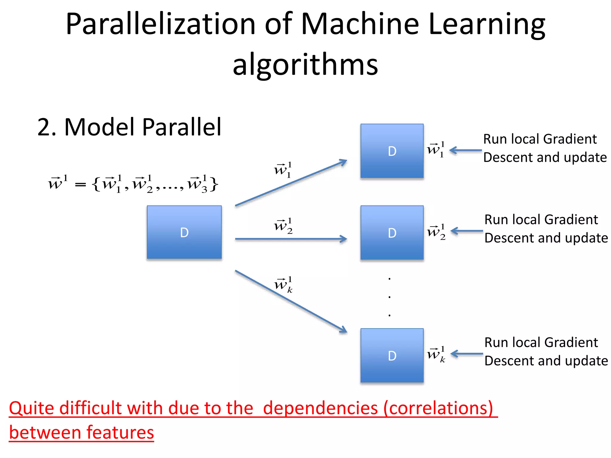
2. Model Parallel
D
D
D
D
.
.
.
Run local Gradient
Descent and update
Run local Gradient
Descent and update
Run local Gradient
Descent and update
Quite difficult with due to the dependencies (correlations)
between features
139.
Parallelization of MachineLearning
algorithms
2. Model Parallel
– Once the dependencies between the parameters
were identified, this is very useful
– Ex. Training large-scale Neural Networks.
http://petuum.github.io/papers/SysAlgTheoryKDD2015.pdf
140.
Parallelization of MachineLearning
algorithms - Implementations
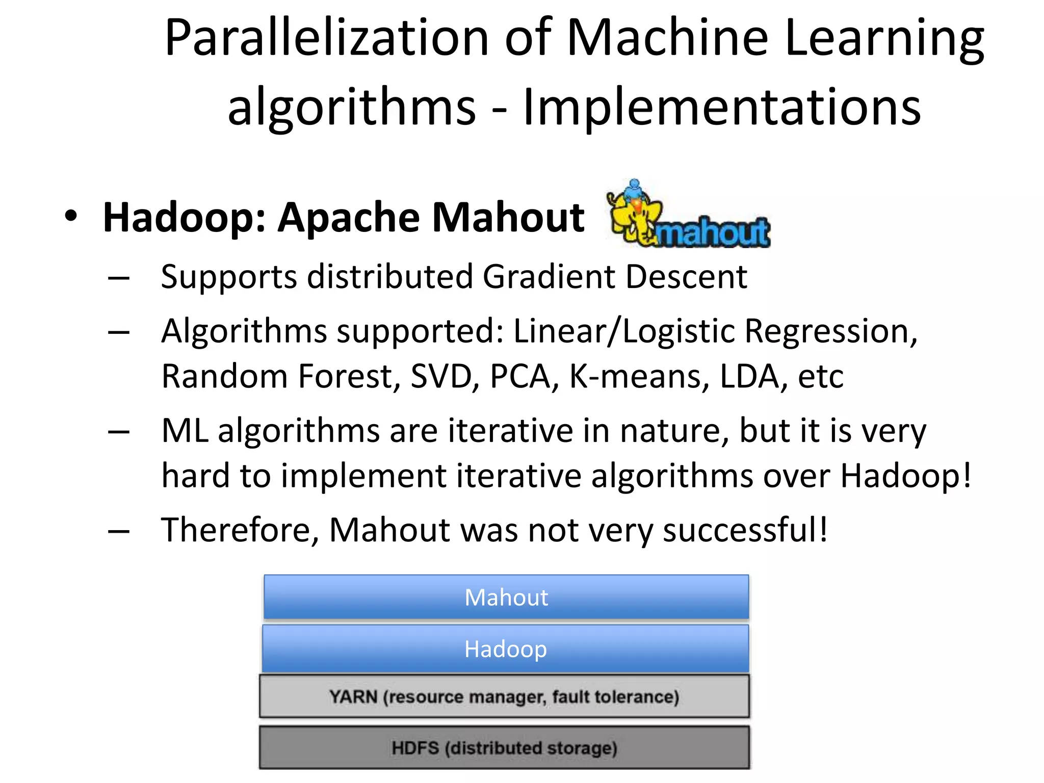
• Hadoop: Apache Mahout
– Supports distributed Gradient Descent
– Algorithms supported: Linear/Logistic Regression,
Random Forest, SVD, PCA, K-means, LDA, etc
– ML algorithms are iterative in nature, but it is very
hard to implement iterative algorithms over Hadoop!
– Therefore, Mahout was not very successful!
Hadoop
Mahout
141.
Parallelization of MachineLearning
algorithms - Implementations
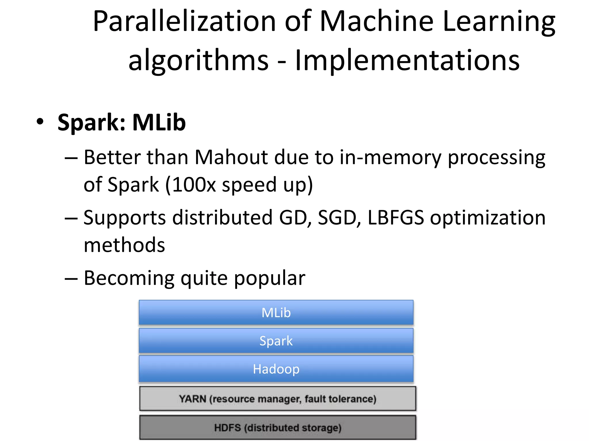
• Spark: MLib
– Better than Mahout due to in-memory processing
of Spark (100x speed up)
– Supports distributed GD, SGD, LBFGS optimization
methods
– Becoming quite popular
Hadoop
Spark
MLib
142.
Parallelization of MachineLearning
algorithms
• Still SAPRK is not designed solely for ML
• Petuum: Distributed ML directly on YARN
• much better optimized low level operations
• CMU Project
http://petuum.github.io/papers/SysAlgTheoryKDD2015.pdf
143.
Parallelization of MachineLearning
algorithms
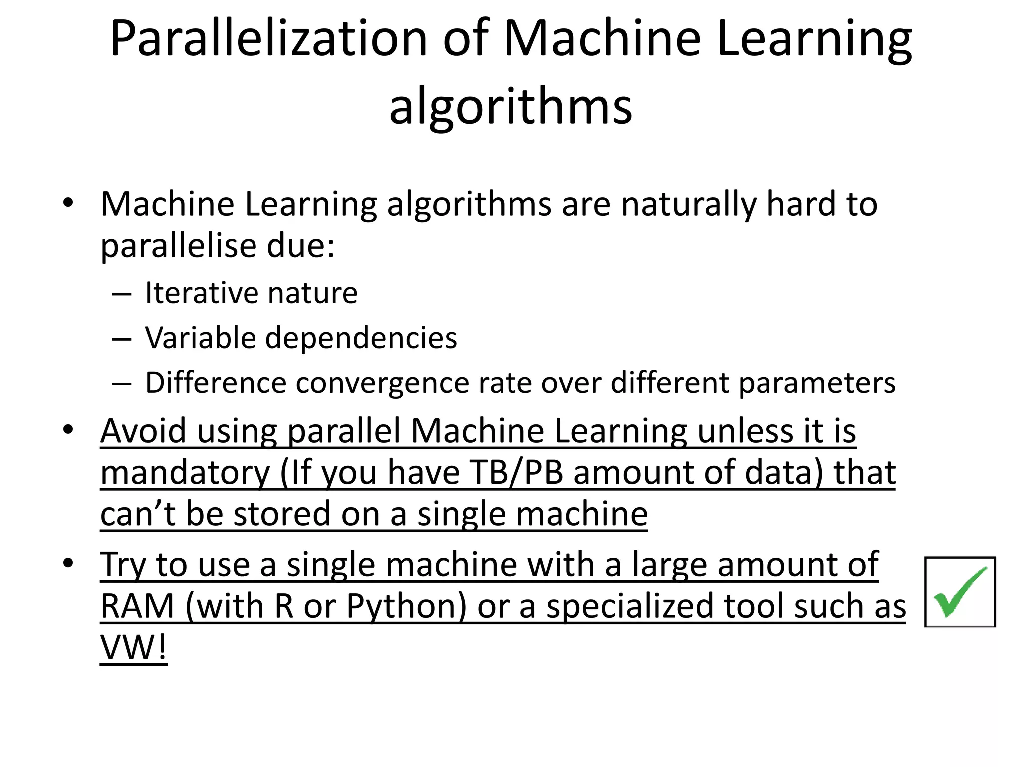
• Machine Learning algorithms are naturally hard to
parallelise due:
– Iterative nature
– Variable dependencies
– Difference convergence rate over different parameters
• Avoid using parallel Machine Learning unless it is
mandatory (If you have TB/PB amount of data) that
can’t be stored on a single machine
• Try to use a single machine with a large amount of
RAM (with R or Python) or a specialized tool such as
VW!
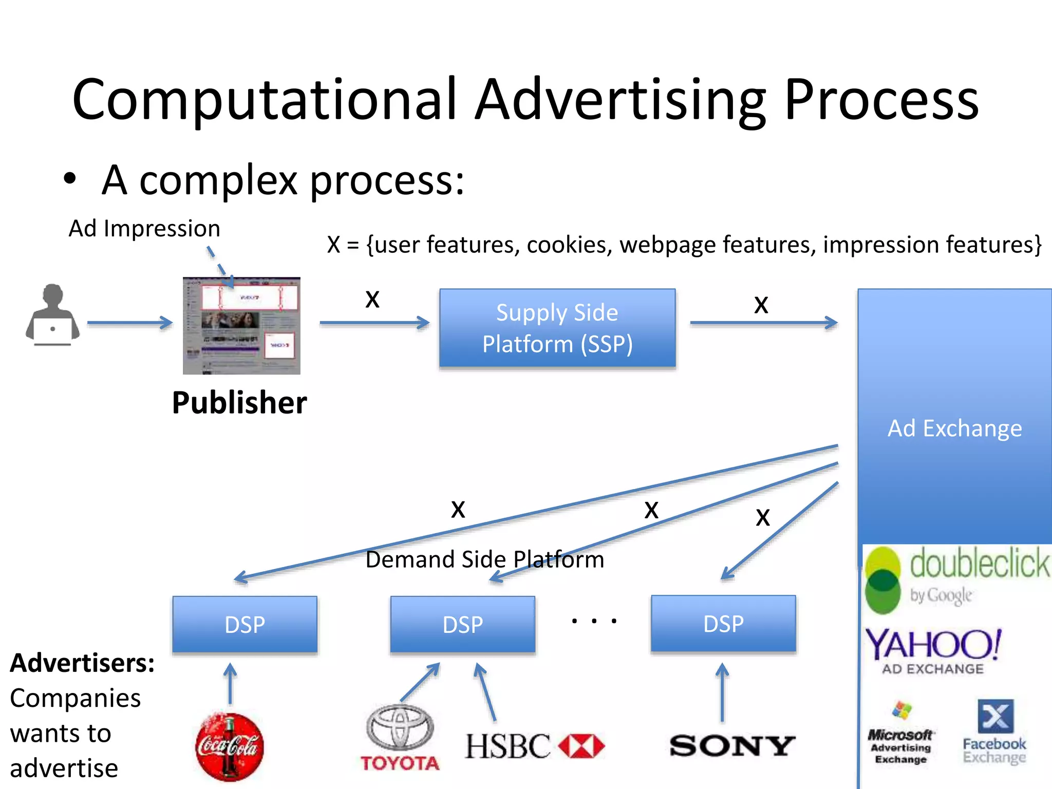
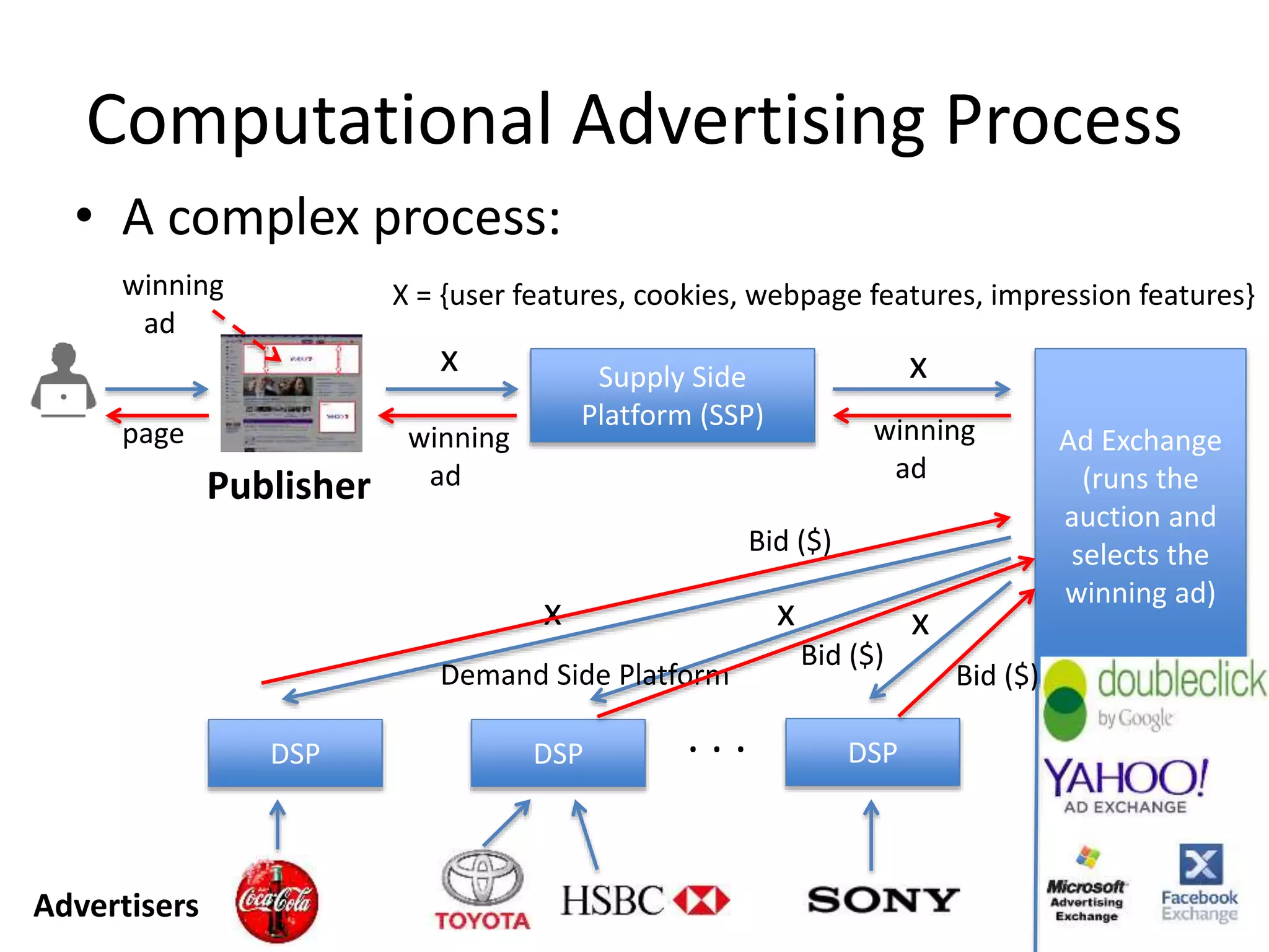
Computational Advertising Process
•A complex process:
Publisher
Supply Side
Platform (SSP)
x
X = {user features, cookies, webpage features, impression features}
Ad Exchange
x
DSPDSPDSP
Demand Side Platform
x x x
. . .
Advertisers:
Companies
wants to
advertise
Ad Impression
149.
Computational Advertising Process
•A complex process:
Publisher
Supply Side
Platform (SSP)
x
Ad Exchange
(runs the
auction and
selects the
winning ad)
x
DSPDSPDSP
Demand Side Platform
x x x
. . .
Advertisers
Bid ($)
Bid ($)
Bid ($)
X = {user features, cookies, webpage features, impression features}
Ad Impression
150.
Computational Advertising Process
•A complex process:
Publisher
Supply Side
Platform (SSP)
x
Ad Exchange
(runs the
auction and
selects the
winning ad)
x
DSPDSPDSP
Demand Side Platform
x x x
. . .
Advertisers
winning
ad
page winning
ad
X = {user features, cookies, webpage features, impression features}
Bid ($)
Bid ($)
Bid ($)
winning
ad
151.
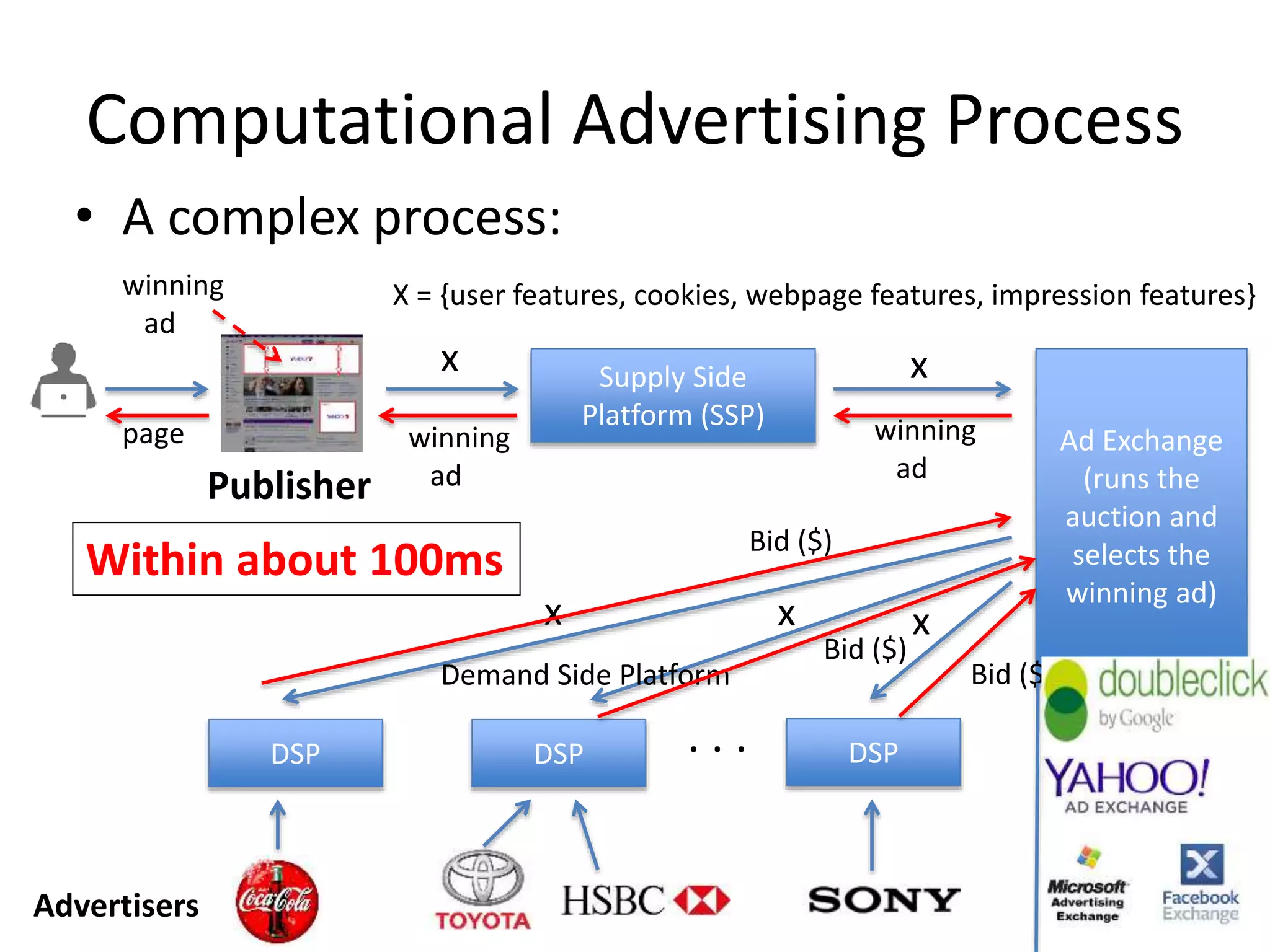
Computational Advertising Process
•A complex process:
Publisher
Supply Side
Platform (SSP)
x
Ad Exchange
(runs the
auction and
selects the
winning ad)
x
DSPDSPDSP
Demand Side Platform
x x x
. . .
Advertisers
Bid ($)
Bid ($)
Bid ($)
winning
ad
page winning
ad
X = {user features, cookies, webpage features, impression features}
Within about 100ms
winning
ad
152.
Computational Advertising Process
•A complex process:
Publisher
Supply Side
Platform (SSP)
x
Ad Exchange
(runs the
auction and
selects the
winning ad)
x
DSPDSPDSP
Demand Side Platform
x x x
. . .
Advertisers
Bid ($)
Bid ($)
Bid ($)
winning
ad
page winning
ad
X = {user features, cookies, webpage features, impression features}
Real-time bidding/
Media Trading
winning
ad
Computational Advertising
How doesthe Ad Exchange/DSP select the winning
ad:
– Let’s say the Ad Exchange is paid if someone clicks on the add
– E(payment/user, ad) = P(click = T/user, ad) * bidding_amount
– Select the Ad which maximizes E(payment/user, ad)
– P(click = T/user, ad) is called Click Through Rate (CTR)
– CTR is estimated by a very large scale model (large-scale logistic
regression model)
DSP
DSP
x
Bid ($)
Ad Exchange
(runs the
auction and
selects the
winning ad)
Bid ($)
x
…
…
155.
Computational Advertising:
Exploration andExploitation
• In Traditional Approach for model-based targeting:
Data Collection
(Randomized Ad Placement)
Train a
model
P(click = T/u, ad)
Use the model for targeting
Exploration Exploitation
• Problems:
• Can’t explore all possible user and add space during exploration
• New users and new ads will appear [change of the features]
• User behavior will change over time [change of P(click = T/u,ad)]
• Can’t waste resources running Random Targeting for a long time
• Therefore, continuous exploration and frequent model update is
needed Exploration
Exploitation
156.
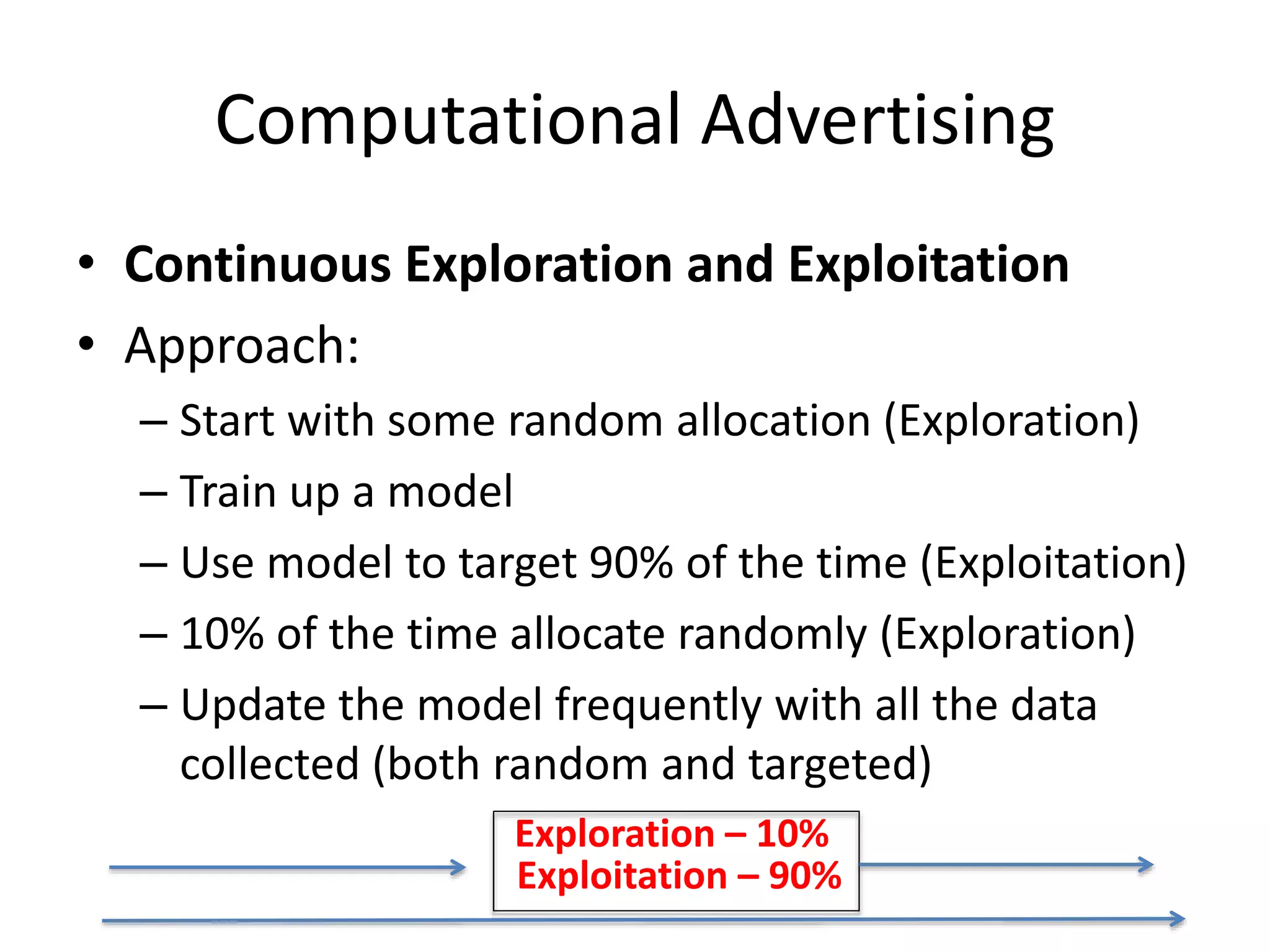
Computational Advertising
• ContinuousExploration and Exploitation
• Approach:
– Start with some random allocation (Exploration)
– Train up a model
– Use model to target 90% of the time (Exploitation)
– 10% of the time allocate randomly (Exploration)
– Update the model frequently with all the data
collected (both random and targeted)
Exploration – 10%
Exploitation – 90%
157.
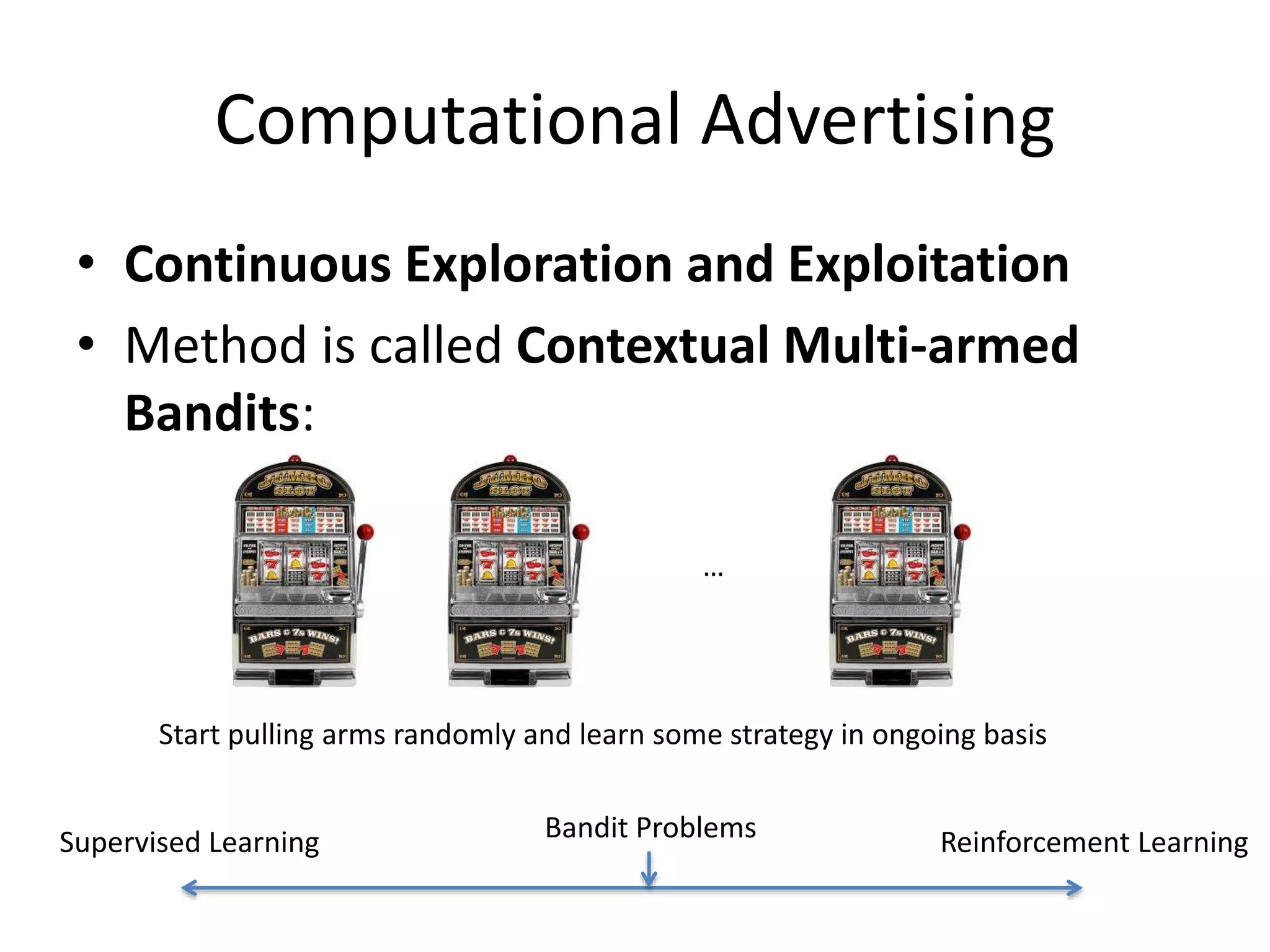
Computational Advertising
• ContinuousExploration and Exploitation
• Method is called Contextual Multi-armed
Bandits:
…
Start pulling arms randomly and learn some strategy in ongoing basis
Supervised Learning Reinforcement LearningBandit Problems
158.
Computational Advertising
• ContinuousExploration and Exploitation
• Most Popular Approach: Thompson Sampling
– Start with some random allocation (Exploration)
– Train up a Bayesian Logistic Regression model
• Assume Gaussian prior for parameters -> Gaussian
posterior for parameters
– For each user, draw a sample of model parameter
values from the posterior and make the
predication – adding randomness at the
exploitation time
W_i
159.
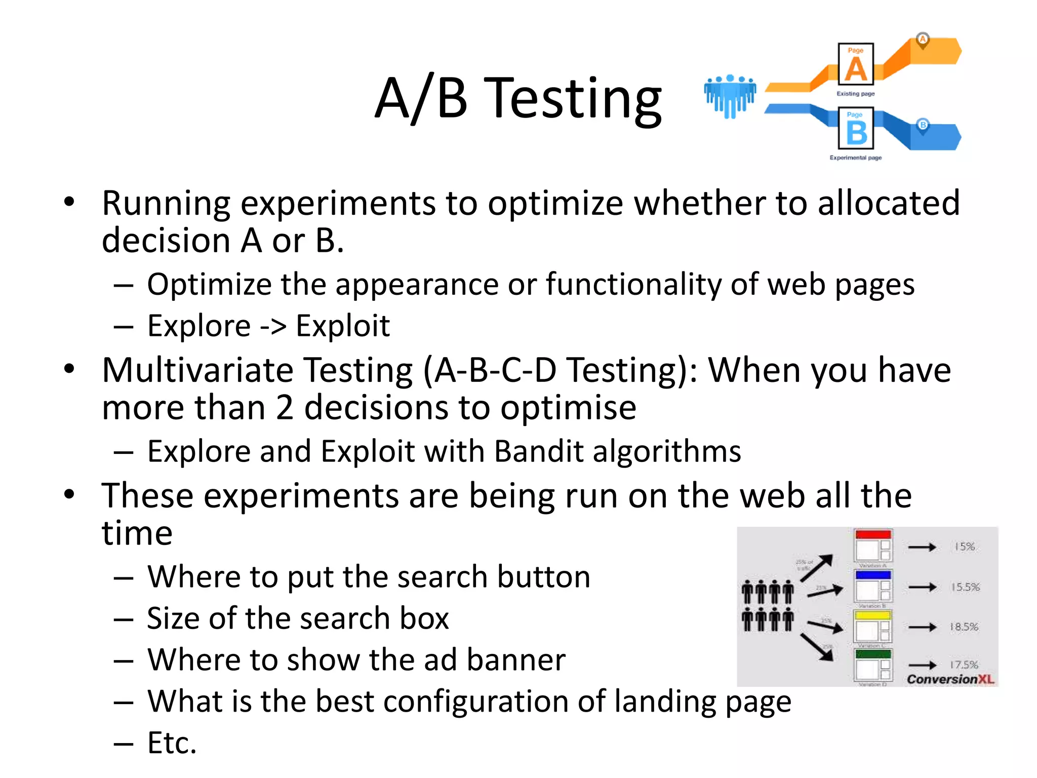
A/B Testing
• Runningexperiments to optimize whether to allocated
decision A or B.
– Optimize the appearance or functionality of web pages
– Explore -> Exploit
• Multivariate Testing (A-B-C-D Testing): When you have
more than 2 decisions to optimise
– Explore and Exploit with Bandit algorithms
• These experiments are being run on the web all the
time
– Where to put the search button
– Size of the search box
– Where to show the ad banner
– What is the best configuration of landing page
– Etc.
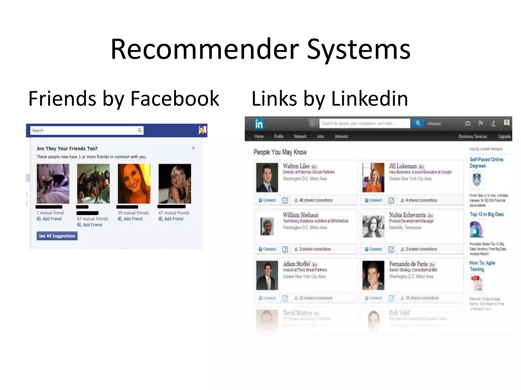
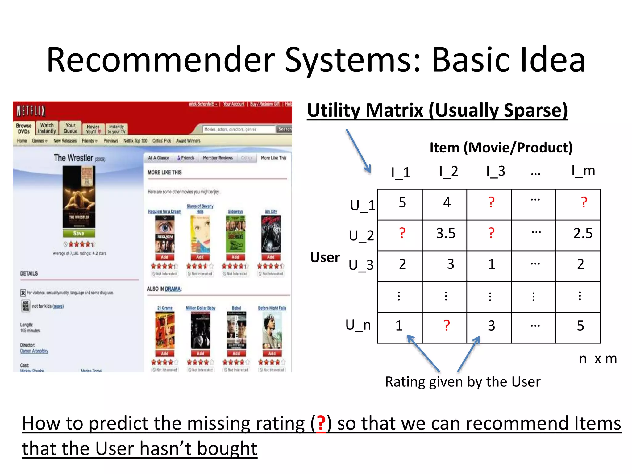
Recommender Systems: BasicIdea
5 4 ? ?
? 3.5 ? 2.5
2 3 1 2
1 ? 3 5
Item (Movie/Product)
User
U_1
U_2
U_3
U_n
I_1 I_2 I_3 I_m…
…
…
…
…
…
…
…
…
…
n x m
Rating given by the User
How to predict the missing rating (?) so that we can recommend Items
that the User hasn’t bought
Utility Matrix (Usually Sparse)
167.
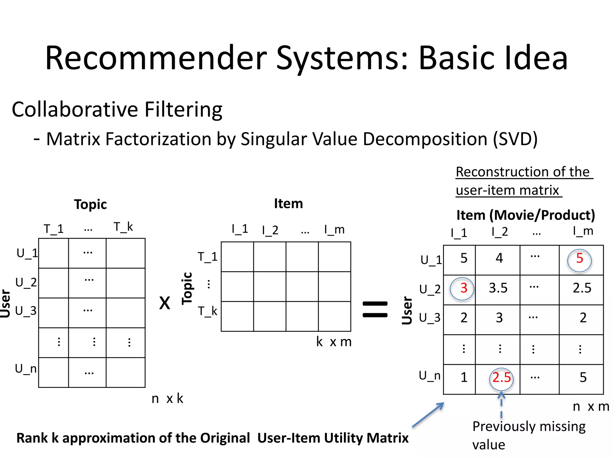
Recommender Systems: BasicIdea
5 4 ?
? 3.5 2.5
2 3 2
1 ? 5
Item (Movie/Product)
User
U_1
U_2
U_3
U_n
I_1 I_2 I_m…
…
…
…
…
…
…
…
…
n x m
Collaborative Filtering
- Matrix Factorization by Singular Value Decomposition (SVD)
Topic
User
U_1
U_2
U_3
U_n
T_1 T_k…
…
…
…
…
…
…
…
n x k
Topic
T_1
T_k
I_1 I_2 I_m…
…
x
k x m
Item
By using the non-missing values of the User-Item Utiity Matrix
168.
Recommender Systems: BasicIdea
5 4 5
3 3.5 2.5
2 3 2
1 2.5 5
Item (Movie/Product)
User
U_1
U_2
U_3
U_n
I_1 I_2 I_m…
…
…
…
…
…
…
…
…
n x m
Collaborative Filtering
- Matrix Factorization by Singular Value Decomposition (SVD)
Topic
User
U_1
U_2
U_3
U_n
T_1 T_k…
…
…
…
…
…
…
…
n x k
Topic
T_1
T_k
I_1 I_2 I_m…
…
x
k x m
=
Rank k approximation of the Original User-Item Utility Matrix
Item
Reconstruction of the
user-item matrix
Previously missing
value
169.
Recommender Systems: BasicIdea
How to solve SVD problem for large Matrices
- Can be solved using a method called Alternating Least Squares
(ALS) via Gradient Descent – (VW Supports this)
- Another useful method is called LDA (Latent Dirichlet Allocation)
used for the Topic Modeling (a Bayesian Model) – (VW
Supports this)
170.
So far….
• BigData Generaztion
• Computing Systems (Storage and Processing)
• Data Processing Algorithms/Cluster
Computing
• Data Analytics/Machine Learning Algorithms
• Large-scale Machine Leanrning
• Applications
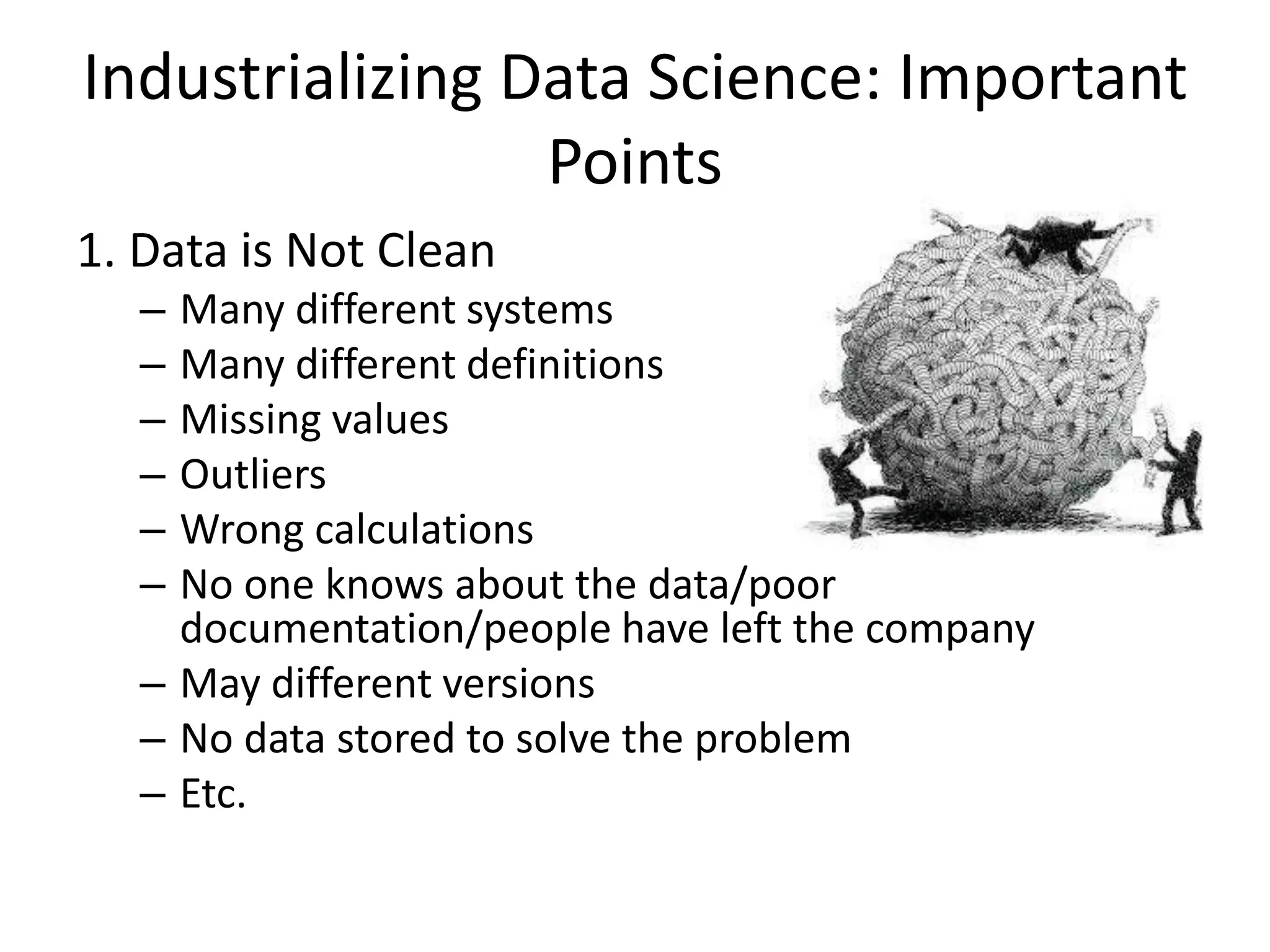
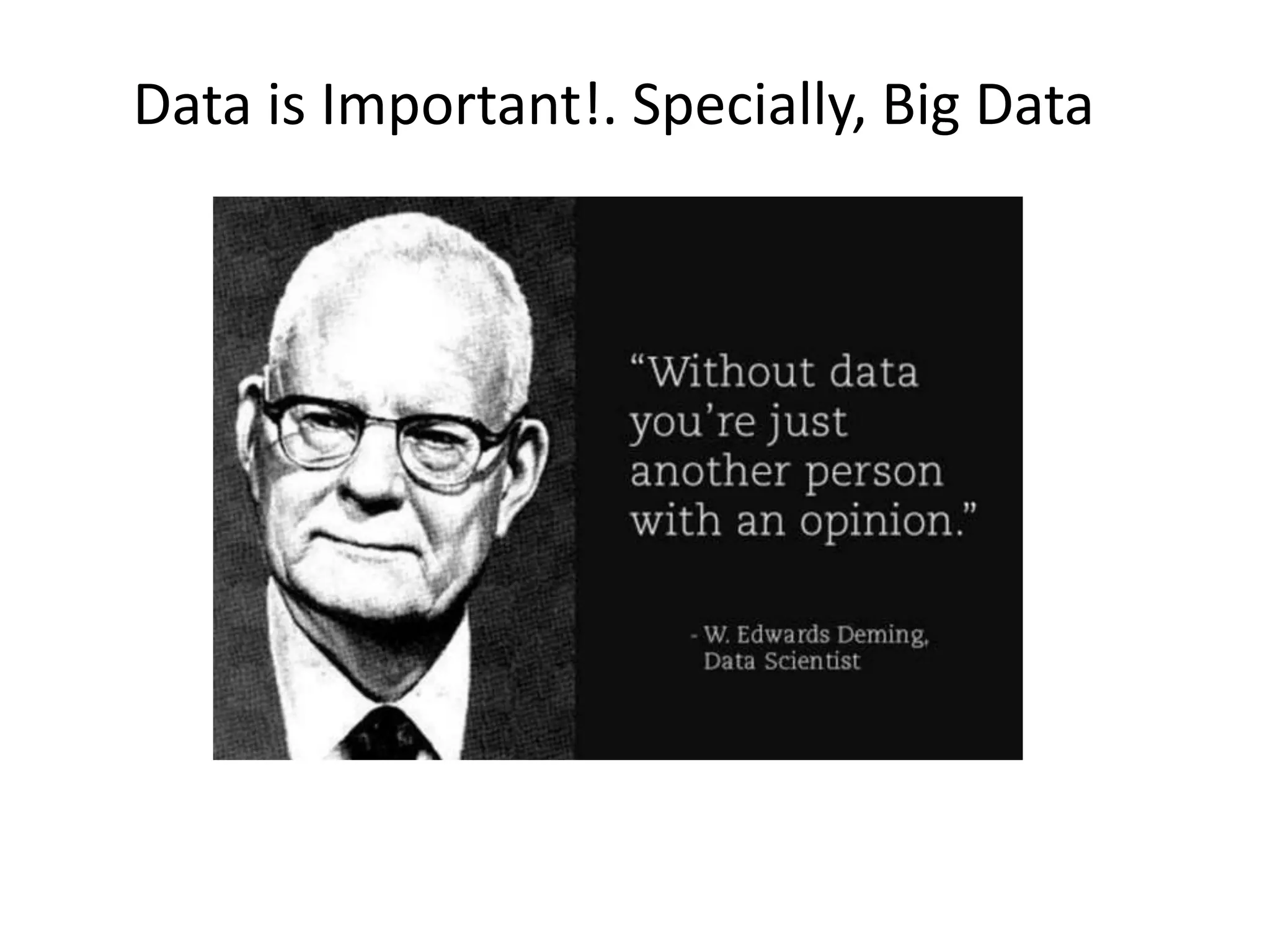
Industrializing Data Science:Important
Points
1. Data is Not Clean
– Many different systems
– Many different definitions
– Missing values
– Outliers
– Wrong calculations
– No one knows about the data/poor
documentation/people have left the company
– May different versions
– No data stored to solve the problem
– Etc.
174.
Industrializing Data Science:Important
Points
2. Correct Problem Definition
– Define the problem to be
solved clearly based on the
available resources:
• Importance of the problem to the
business
• Data
• Systems (Hardware and software)
• People
175.
Industrializing Data Science:Important
Points
3. Don’t afraid to get Your Hands Dirty with the
Data
– Machine Learning is not magic
– The data has to be interrogated in different ways to get the work
done
• Data cleaning
• Visualization
• Feature engineering
• Feature pre-processing
• Model training
• Model validation
• Model diagnostic
• Model productionizing
• Performance monitoring
• Model updating
176.
Industrializing Data Science:Important
Points
4. Select a Suitable Modeling Method:
– There is no a single perfect ML algorithm that works
for all the problems: No Free Lunch Theorem
– Modeling approach has to be selected based on:
• Problem we are trying to solve
• Complexity of the problem
• Size of the data
• Availability of the resources: Systems, Time, People
• Etc.
177.
Industrializing Data Science:Important
Points
5. Model Validation and Diagnostics
– Test for overfitting
– Proper hyper-parameter tuning
– Proper validation
• Label leakage problem
– Some database fields can get overwritten after the
label is collected
178.
Industrializing Data Science:Important
Points
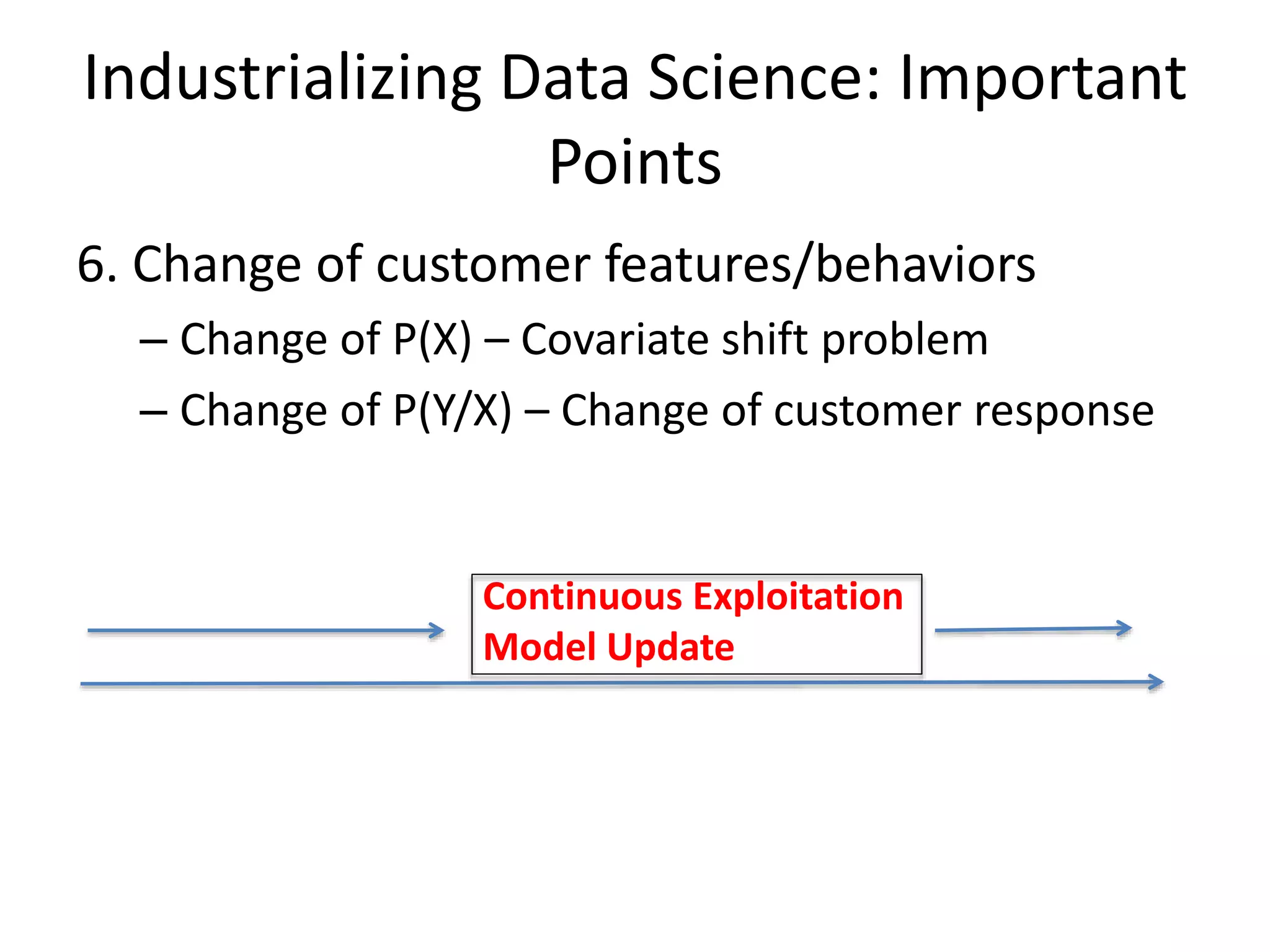
6. Change of customer features/behaviors
– Change of P(X) – Covariate shift problem
– Change of P(Y/X) – Change of customer response
Continuous Exploitation
Model Update
179.
Industrializing Data Science:Important
Points
7. Experimental Design and Sample Bias
– For some problems, the randomized experiments
have to be set up to collect data:
• Personalized interventions such as marketing
campaigns, product recommendations, price
adjustments etc.
Control Group Random Treatment Group
All the groups should be statistically identical with respect to all the
variables of interest
Population
of customers
180.
Industrializing Data Science:Important
Points
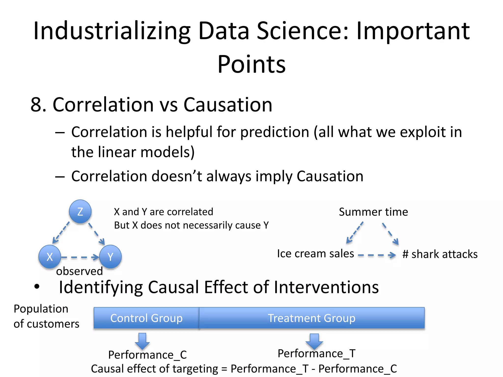
8. Correlation vs Causation
– Correlation is helpful for prediction (all what we exploit in
the linear models)
– Correlation doesn’t always imply Causation
• Identifying Causal Effect of Interventions
Control Group Treatment Group
Population
of customers
Z
X Y
observed
X and Y are correlated
But X does not necessarily cause Y
Ice cream sales # shark attacks
Summer time
Performance_C Performance_T
Causal effect of targeting = Performance_T - Performance_C
Industrializing Data Science:Important
Points
• Statistical Significance of Measurements
Control Group Treatment Group
Performance_C = $30.55 Performance_T = $31.05
Causal effect of targeting = Performance_T - Performance_C = $0.50 = average
uplift per customer
• If there are 2M customers = Total Uplift = $1M
• Assume the campaign cost is $300k (Net uplift of 700k)
• Is this Significant (Is it worth running this campaign)?
• Do we have enough information to answer this question? TC
$30.55
$31.05
183.
Industrializing Data Science:Important
Points
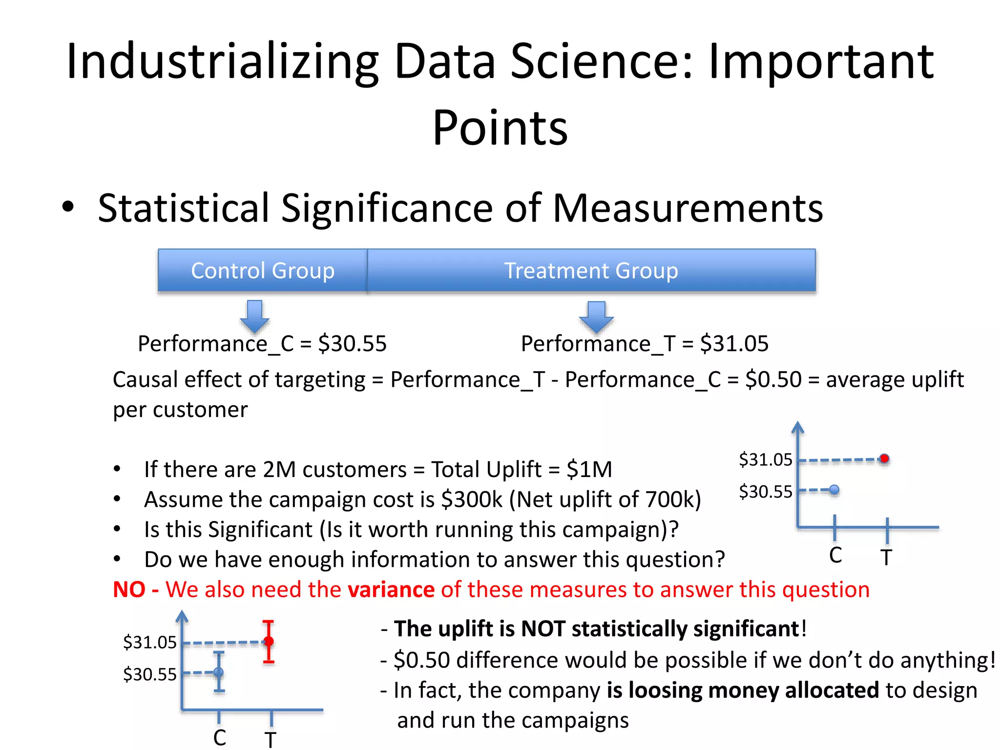
• Statistical Significance of Measurements
Control Group Treatment Group
Performance_C = $30.55 Performance_T = $31.05
Causal effect of targeting = Performance_T - Performance_C = $0.50 = average uplift
per customer
• If there are 2M customers = Total Uplift = $1M
• Assume the campaign cost is $300k (Net uplift of 700k)
• Is this Significant (Is it worth running this campaign)?
• Do we have enough information to answer this question?
NO - We also need the variance of these measures to answer this question
TC
$30.55
$31.05
TC
$30.55
$31.05
- The uplift is NOT statistically significant!
- $0.50 difference would be possible if we don’t do anything!
- In fact, the company is loosing money allocated to design
and run the campaigns
184.
Industrializing Data Science:Important
Points
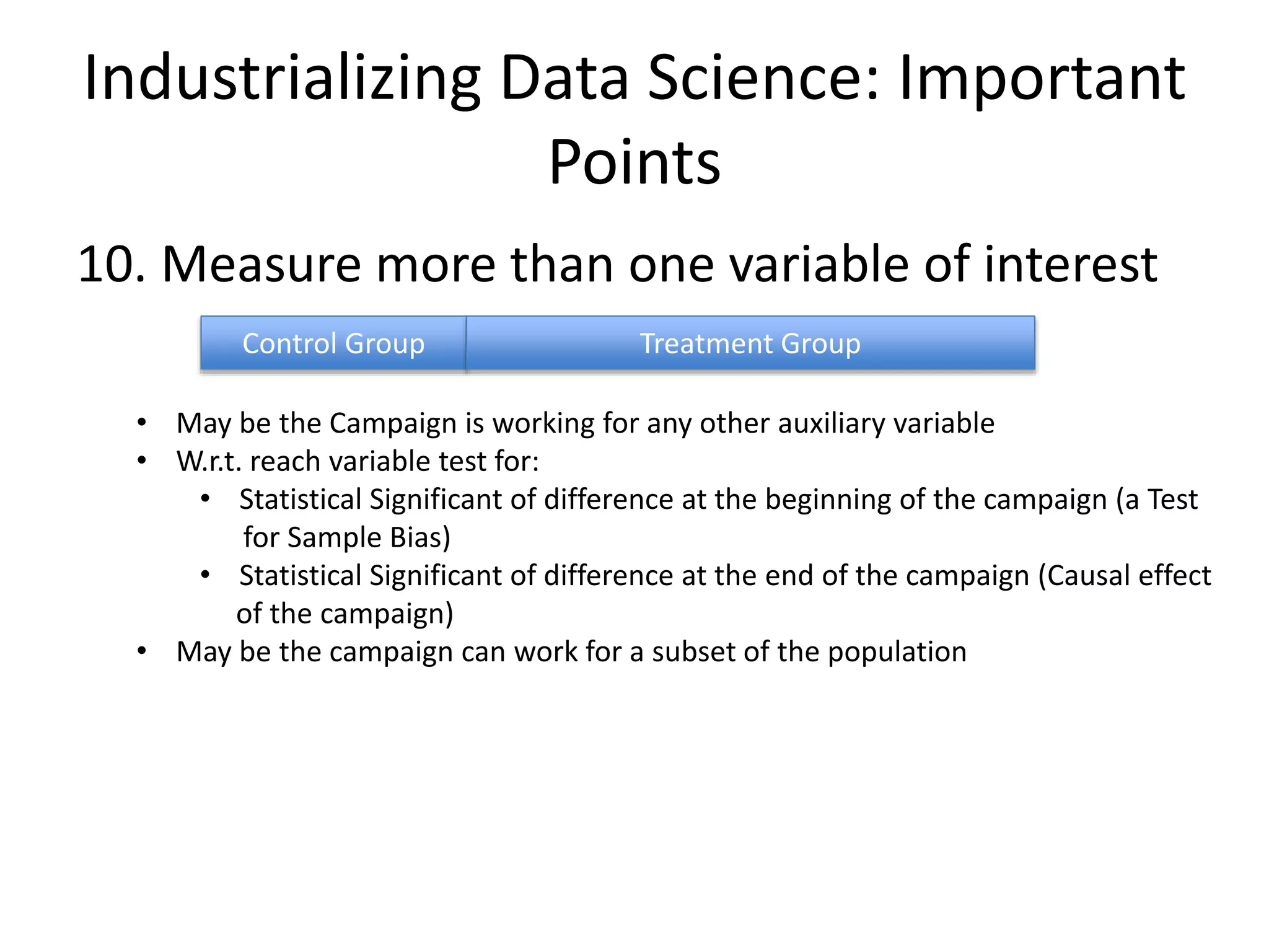
10. Measure more than one variable of interest
Control Group Treatment Group
• May be the Campaign is working for any other auxiliary variable
• W.r.t. reach variable test for:
• Statistical Significant of difference at the beginning of the campaign (a Test
for Sample Bias)
• Statistical Significant of difference at the end of the campaign (Causal effect
of the campaign)
• May be the campaign can work for a subset of the population
185.
Industrializing Data Science:Important
Points
11. Different between Software and Data
Science projects
– Outcome of a Software project is more certain
and deterministic
– Outcome of a Data Science project is less certain
or non-deterministic
Business
Problem/Requirements
Final Deliverable
Software
System
Business
Problem/Requirements
Final Deliverable
Software,
Slide deck,
Report
Data brings in the uncertainty
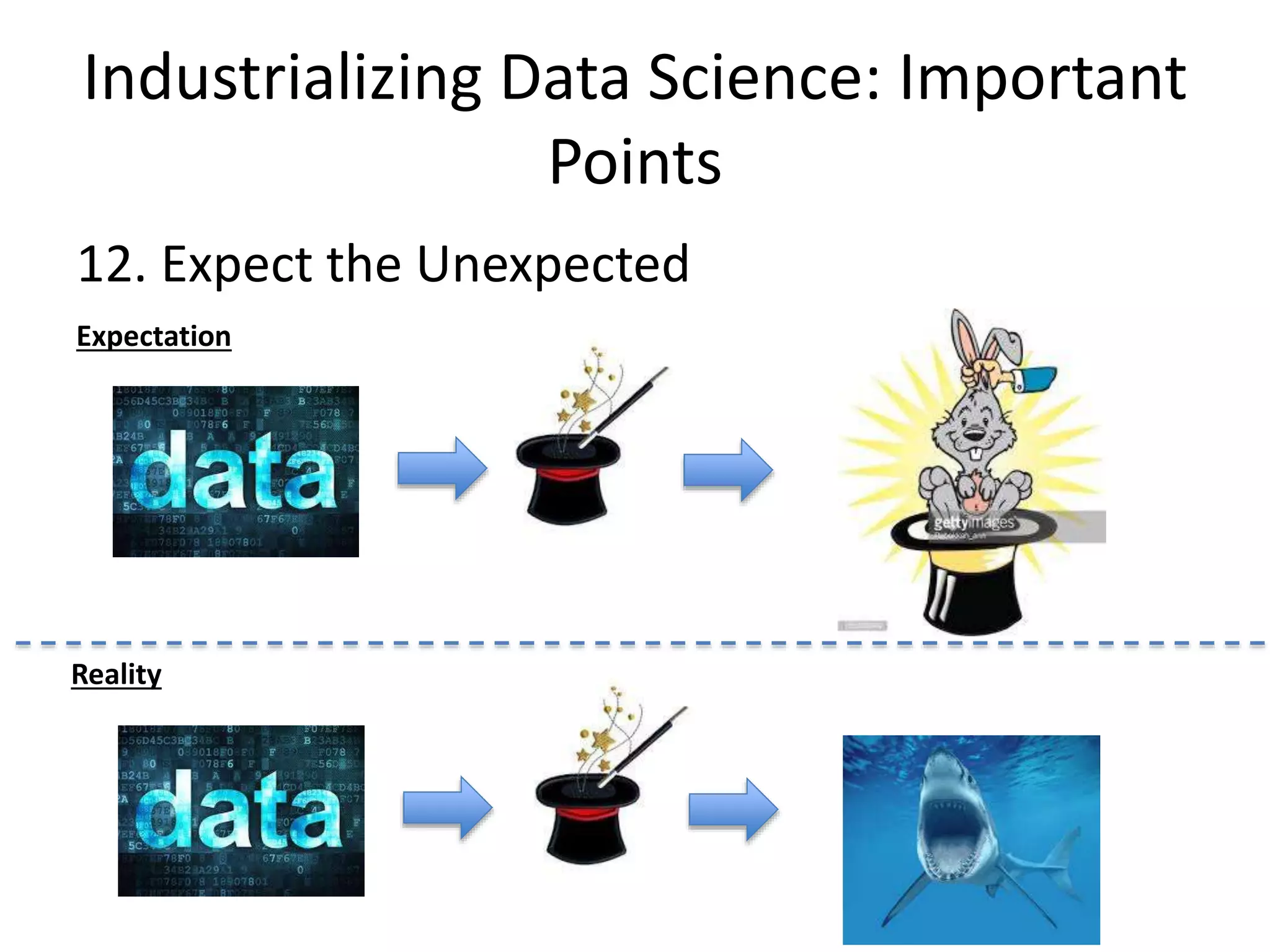
Industrializing Data Science:Important
Points
13. Communication Issues with the business
- C-level people (CEO, CIO, CFO, etc.)
- Marketing people
- Statisticians
- S/W Engineers
- etc.
Data
Scientist
Data
Engineer
Business problems
Available Resources
Results
Challenges:
• Convincing Business and IT people to start Data Science projects
• Communication of the ‘Science/Statistics’ back to the
Business can get very challenging!
• Problem of Statistical/Business Literacy
and being Narrow Minded (Not Open to Listen to each other)
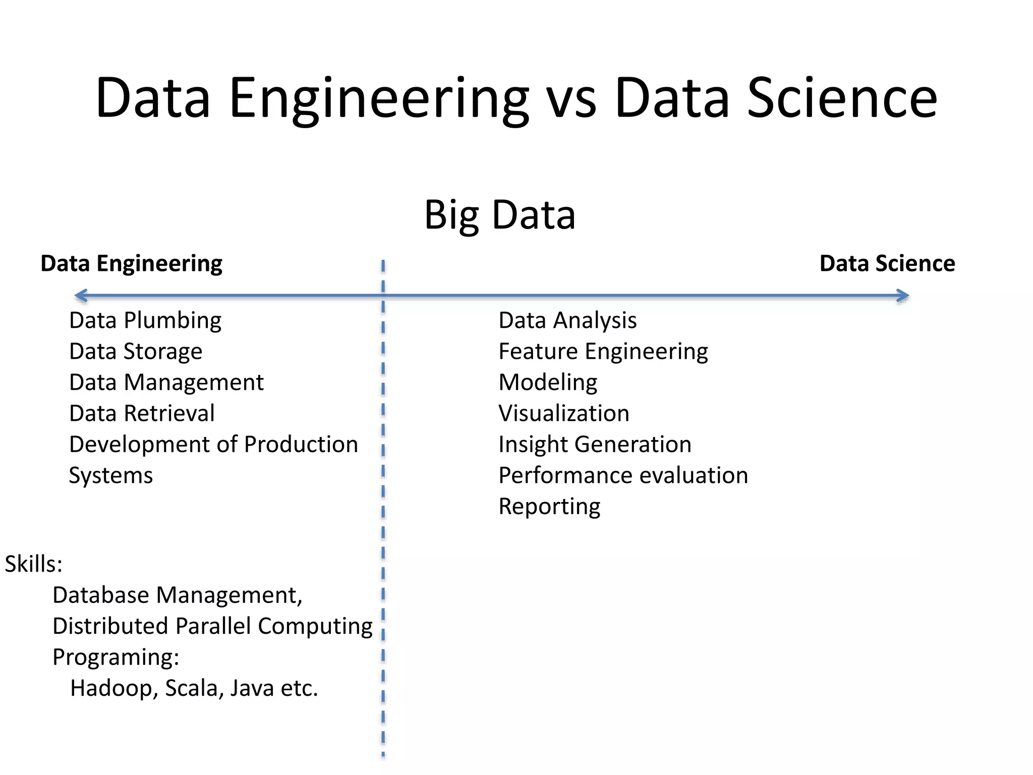
Data Engineering vsData Science
Big Data
Data Engineering
Data Plumbing
Data Storage
Data Management
Data Retrieval
Development of Production
Systems
Data Science
Skills:
Database Management,
Distributed Parallel Computing
Programing:
Hadoop, Scala, Java etc.
Data Analysis
Feature Engineering
Modeling
Visualization
Insight Generation
Performance evaluation
Reporting
190.
How to becomea Data Scientist
• Skills:
– Statistics
– Machine Learning
– Mathematics (Optimisation, Functional Analysis,
Linear Algebra, etc.)
• Programing Skills:
– Python, R, Hadoop, Spark, etc
• Written and Verbal Communication and Presentation
skills
• Creativity
191.
Some Resources
• Startwith Googling
• Data Science Courses: Online – Cousera
– Standford Uni, UC Berkeley, Washington Uni.
• Machine Learning:
– @ Standford Uni by Andrew Ng, @ Oxford by Nando de Freitas, @
CMU by Alex Smola
• Large Scale ML:
– NUY Large Scale ML Course - 2013
– Alex Smola’s course at UC Berkeley – 2012
• Useful websites:
– http://www.datasciencecentral.com/
– http://www.kdnuggets.com/
– Large-scale ML: FastML, Hunch.net
• Conferences: KDD, ICML, NIPS, etc.
192.
A little bitabout Ambiata
• Current Status:
– Serving Teir 1 Industries in Australia:
• Banks
• Telecommunication
• Supermarkets
• Insurance
• Media
• Etc
– Touching millions of customers everyday with personalized
interventions driving millions of revenue for organizations
– Hitting the global market soon
– 20 Engineers + 10 Data Scientists


![Process of Data Analytics
2. Process of Data Analytics
Retrieval
Data pre-processing/cleaning
Data Analysis
[~80% of the time spent on making the data ready for the analysis]](https://image.slidesharecdn.com/introdatascienceshare-160507131612/75/Big-Data-and-Data-Science-The-Technologies-Shaping-Our-Lives-75-2048.jpg)


![How do we tune W?
• Model: , where is the estimated value
of under the model:
• Loss Function:
– difference between actual label and the predicted label
• In Model Training:
ˆyi = ˆf (xi,w)
loss_ fn = L(yi, ˆyi ) = L(yi, ˆf (xi,w))
w*
= arg_min
w
[loss_ fn]= arg_min
w
[L(yi, f (xi,w))]
ˆyi
yi](https://image.slidesharecdn.com/introdatascienceshare-160507131612/75/Big-Data-and-Data-Science-The-Technologies-Shaping-Our-Lives-96-2048.jpg)


![Vowpal Wabbit (VW)
• Constant memory footprint
– VW only maintains the model parameter vector (weight vector) in the
memory and all the data is on the disk
– VW reads one training instance at a time into memory when calculating
the gradient – so you can have Billions of instances!
– For multiple passes over a dataset VW creates a binary cache version of
the input data file -> much faster read in from the disk
• Feature Hashing
– Feature names are hashed (32-bit murmurHash function) to
map into the locations of the weight vector in the memory
– Fast updates and efficient memory usage (no need to maintain a
feature dictionary)
– Default is 18 bit hash function [max is 32bits ~ 4 billion
features!]
Very Efficient Memory Management:](https://image.slidesharecdn.com/introdatascienceshare-160507131612/75/Big-Data-and-Data-Science-The-Technologies-Shaping-Our-Lives-127-2048.jpg)
![Vowpal Wabbit (VW)
• Main input data format is text files or stdin
• Sparse representation of features:
[Label] [Importance weight] [id]|Namespace f_name1:val1 …|Namespace f_name1:val1 … |…](https://image.slidesharecdn.com/introdatascienceshare-160507131612/75/Big-Data-and-Data-Science-The-Technologies-Shaping-Our-Lives-128-2048.jpg)


![Computational Advertising:
Exploration and Exploitation
• In Traditional Approach for model-based targeting:
Data Collection
(Randomized Ad Placement)
Train a
model
P(click = T/u, ad)
Use the model for targeting
Exploration Exploitation
• Problems:
• Can’t explore all possible user and add space during exploration
• New users and new ads will appear [change of the features]
• User behavior will change over time [change of P(click = T/u,ad)]
• Can’t waste resources running Random Targeting for a long time
• Therefore, continuous exploration and frequent model update is
needed Exploration
Exploitation](https://image.slidesharecdn.com/introdatascienceshare-160507131612/75/Big-Data-and-Data-Science-The-Technologies-Shaping-Our-Lives-155-2048.jpg)


![Big Data [sorry] & Data Science: What Does a Data Scientist Do?](https://cdn.slidesharecdn.com/ss_thumbnails/dslatcloudmsevent20130125-130126065651-phpapp01-thumbnail.jpg?width=640&height=640&fit=bounds)