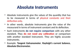
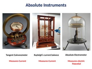
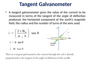
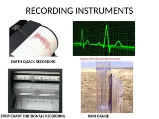
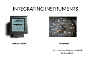
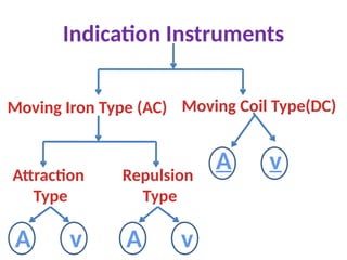
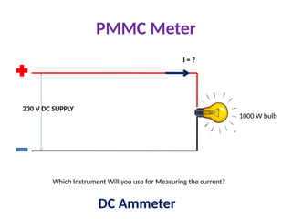
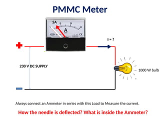
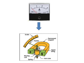
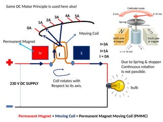
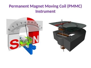
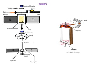
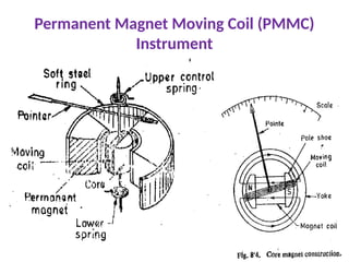
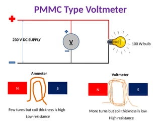
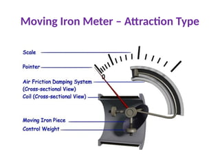
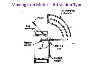
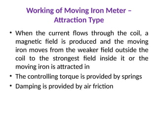
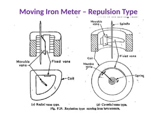
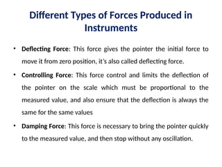
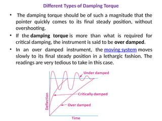
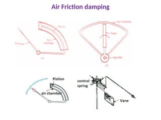
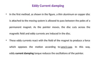
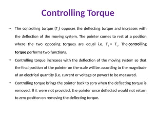
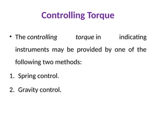
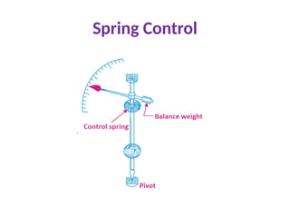
MODULE - 3
MEASUREMENTS AND INSTRUMENTATION
Primary instruments, secondary instruments,
fundamental torques of an instrument, types of damping
torque, controlling torque and defecting torques. Working
principle of PMMC meters and moving iron meters
Measurements
What is Measurement?
• The measurement of a given quantity is
essentially an act or the result of comparison
between the quantity (Whose magnitude is
unknown) and a predefined standard. Since
two quantities are compared the result is
expressed in numerical values
• Instruments generally involved
Types of Instruments
• Absolute Instruments
• Secondary Instruments
Absolute Instruments
• Absolute instruments give the values of the quantity that has
to be measured in terms of physical constants and their
deflection only.
• In other words, absolute instruments give the value of the
measurand in terms of instrument constant and its deflection.
• Such instruments do not require comparison with any other
standard. They do not need any calibration or comparison
with another standard instrument. They are highly accurate
instruments.
• Example: Tangent Galvanometer, Rayleigh’s current balance,
Absolute Electrometer.
Absolute Instruments
Absolute Electrometer
Tangent Galvanometer Rayleigh’s current balance
Measures Current Measures Current Measures electric
Potential
Tangent Galvanometer
• A tangent galvanometer gives the value of the current to be
measured in terms of the tangent of the angle of deflection
produced, the horizontal component of the earth’s magnetic
field, the radius and the number of turns of the wire used.
Absolute Instruments
Definition:
Absolute instruments are those which give the value of
the quantity to be measured in terms of the constant
of the instrument and their deflection only.
• No previous calibration or comparison is necessary in
their case
• Ex: Tangent Galvanometer which gives the value of
current in terms of the tangent deflection produced by
the current and of the radius and number of turns of
wire used and the horizontal component of earth’s field
Secondary Instruments
• Secondary instruments are so constructed that the deflection
of such instruments gives the magnitude of the electrical
quantity to be measured directly.
• These instruments are required to be calibrated by
comparison with either an absolute instrument or with
another secondary instrument, which has already been
calibrated before the use.
• They are defined as the instruments that give a ready
measure of the quantities with the help of graduated scales.
• Example: Ammeter, Voltmeter, Wattmeter
Secondary Instruments
Definition:
Secondary instruments are those which give
the value of the quantity to be measured in
terms of their deflection only.
• Previous calibration or comparison is
necessary in their case
Classification of Secondary Instruments
• Indicating Instruments
– indicates instantaneous values of current or voltage
Ex: Ammeters, Voltmeters and Wattmeter
• Recording Instruments
– Continuous record of the variations of voltage, current or
power over a selected period of time.
Ex: inked pen moves on a chart or graph, ECG
• Integrating Instruments
– summation of instantaneous values are recorded
Ex: Energy Meter or Watt-Hour Meter
INDICATING INSTRUMENTS
RECORDING INSTRUMENTS
EARTH QUACK RECORDING
STRIP CHART FOR SIGNALS RECORDING RAIN GAUGE
INTEGRATING INSTRUMENTS
ENERGY METER Odometer
Recorded the distance travelled
By the vehicle.
Indication Instruments
Moving Iron Type (AC) Moving Coil Type(DC)
Attraction
Type
Repulsion
Type
A v A v
A v
PMMC Meter
230 V DC SUPPLY
I = ?
1000 W bulb
Which Instrument Will you use for Measuring the current?
DC Ammeter
PMMC Meter
230 V DC SUPPLY
I = ?
1000 W bulb
Always connect an Ammeter in series with this Load to Measure the current.
5A
How the needle is deflected? What is inside the Ammeter?
230 V DC SUPPLY
I = 0A
bulb
N S
0A
1A
2A
3A 4A 5A
I=1A
I=3A
Coil rotates with
Respect to its axis.
Permanent Magnet
Moving Coil
Permanent Magnet + Moving Coil = Permanent Magnet Moving Coil (PMMC)
Same DC Motor Principle is used here also!
Due to Spring & stopper
Continuous rotation
Is not possible.
I
Permanent Magnet Moving Coil (PMMC)
Instrument
(PMMC)
Permanent Magnet Moving Coil (PMMC)
Instrument
PMMC Type Voltmeter
230 V DC SUPPLY
100 W bulb
V
N S
Few turns but coil thickness is high
Ammeter
N S
More turns but coil thickness is low
Voltmeter
Low resistance High resistance
PMMC Instrument Working
D:AcademicsBEEE_BEEMBEEMEUnit V videosMETERS
Torque Equation of PMMC Instruments
N S
B
N- Turns
L
d I-current
Let
N- Number of Turns in the coil
I – Current flowing through the coil
L – Length of the coil
d- breadth of the coil
B – Magnetic field in the permanent magnet
The deflecting torque produced in coil:
Td = N*B*L*d*I -------- 1
Control torque developed by the spring:
Tc = kθ ---------- 2
Equation 1 = Equation 2
Td = Tc
NBLdI = kθ
I = kθ / NBLd
What will happen in these cases?
230 V DC SUPPLY
V
230 V DC SUPPLY
I = ?
A
In both the cases,
Meter will show the
Deflection in Opposite
Direction!
Always we must
Take care about the
Meter Polarity !
D:AcademicsBEEE_BEEMBEEMEUnit V videosMETERS
Moving Iron Meter – Attraction Type
Working of Moving Iron Meter –
Attraction Type
• When the current flows through the coil, a
magnetic field is produced and the moving
iron moves from the weaker field outside the
coil to the strongest field inside it or the
moving iron is attracted in
• The controlling torque is provided by springs
• Damping is provided by air friction
Moving Iron Meter – Repulsion Type
• In the repulsion type, there are two vanes
inside the coil one fixed and other movable.
• These are similarly magnetized when the
current flows through the coil and there is a
force of repulsion between the two vanes
resulting in the movement of the moving
vane.
Working of Moving Iron Meter –
Repulsion Type
D:AcademicsBEEE_BEEMBEEMEUnit V videosMETERS
Torque Equation of MI Instruments
• Considering the energy relations when there is
a small increment in current supplied to the
instrument
• When this happens there will be a small
deflection dθ and some mechanical work done
• Let Td = Deflecting Torque
• Therefore, Mechanical Work done = Td*dθ
• Let L- Instrument Inductance
• Θ – Deflection of pointer
• dI – small change in current
• dθ – small change in deflection due to dI
• Then the applied voltage is given by
Torque Equation of Moving Iron Instruments.doc
x
DC Meters and AC Meters
Uniform scale
Initially crowded or cramped
And non- uniform scale
Ɵ α I2
Ɵ α I
Why MI meter has non-uniform scale?
• The deflection of needle of moving iron
instrument is given in terms of rms value of
voltage or current. As the angular deflection
of Moving Iron Instrument is proportional to
square of operating current, therefore the
instrument has basically square law response.
Due to this square law response, the Moving
Iron Instrument Scale is non-uniform.
Ɵ α I2
Different Types of Forces Produced in
Instruments
• Deflecting Force: This force gives the pointer the initial force to
move it from zero position, it’s also called deflecting force.
• Controlling Force: This force control and limits the deflection of
the pointer on the scale which must be proportional to the
measured value, and also ensure that the deflection is always the
same for the same values
• Damping Force: This force is necessary to bring the pointer quickly
to the measured value, and then stop without any oscillation.
Different Types of Damping Torque
• The damping torque should be of such a magnitude that the
pointer quickly comes to its final steady position, without
overshooting.
• If the damping torque is more than what is required for
critical damping, the instrument is said to be over damped.
• In an over damped instrument, the moving system moves
slowly to its final steady position in a lethargic fashion. The
readings are very tedious to take in this case.
Damping Torque
• A damping torque is produced by a damping or stopping force
which acts on the moving system only when it is moving and
always opposes its motion. Such a torque is necessary to bring
the pointer to rest quickly.
• If there is no damping torque, then the pointer will keep
moving to and fro about its final deflected position for some
time before coming to rest, due to the inertia of the moving
system.
Methods of Producing Damping torque
• Air friction damping
• Fluid friction damping
• Eddy current damping
Air Friction damping
Air friction damping
• Arrangements of air friction damping are shown in fig. (a) and fig. (b). In the
arrangement shown in fig (a), a light aluminum piston is attached to the
spindle that carries the pointer and moves with a very little clearance in a
rectangular or circular air chamber closed at one end.
• The cushioning action of the air on the piston damps out any tendency of
the pointer to oscillate about the final deflected position. This method is
not favored these days and the one shown in fig. (b) is preferred.
• In this method, one or two light aluminum vanes are attached to the same
spindle that carries the pointer. As the pointer moves, the vanes swing and
compress the air. The pressure of compressed air on the vanes provides the
necessary damping force to reduce the tendency of the pointer to oscillate.
Fluid friction damping
• In this method, discs or vanes attached to the spindle of the moving
system are kept immersed in a pot containing oil of high viscosity. As the
pointer moves, the friction between the oil and vanes opposes the motion
of the pointer and thus necessary damping is provided.
• The fluid friction damping method is not suitable for portable instruments
because of the oil contained in the instrument. In general, fluid friction
damping is not employed in indicating instrument, although one can find
its use in Kelvin electrostatic voltmeter.
Eddy Current damping
• In the first method, as shown in the figure, a thin aluminum or copper disc
is attached to the moving system is allowed to pass between the poles of a
permanent magnet. As the pointer moves, the disc cuts across the
magnetic field and eddy currents are induced in the disc.
• These eddy currents react with the field of the magnet to produce a force
which opposes the motion according to Lenz’s Law. In this way,
eddy current damping torque reduces the oscillations of the pointer.
Controlling Torque
• The controlling torque (Tc) opposes the deflecting torque and increases with
the deflection of the moving system. The pointer comes to rest at a position
where the two opposing torques are equal i.e. Td = Tc. The controlling
torque performs two functions.
• Controlling torque increases with the deflection of the moving system so that
the final position of the pointer on the scale will be according to the magnitude
of an electrical quantity (i.e. current or voltage or power) to be measured.
• Controlling torque brings the pointer back to zero when the deflecting torque is
removed. If it were not provided, the pointer once deflected would not return
to zero position on removing the deflecting torque.
Controlling Torque
• The controlling torque in indicating
instruments may be provided by one of the
following two methods:
1. Spring control.
2. Gravity control.
Spring Control
Spring Control
• This is the most common method of providing controlling torque, in
electrical instruments. A spiral hairspring made of some non-magnetic
material like phosphor bronze is attached to the moving system of the
instrument as shown in the figure.
• Springs also serve the additional purpose of leading current to the moving
system (i.e. operating coil). With that deflection of the pointer, the spring
is twisted in the opposite direction. This twist in the spring provides the
controlling torque.
Spring Control
• Since the torsion torque of a spiral spring is proportional to the angle of
twist, the controlling torque (Tc ) is directly proportional to the angle of
deflection of pointer (θ) i.e. Tc α θ. The pointer will come to rest at a
position where controlling torque is equal to the deflecting torque i.e.
Td =Tc.
• In an instrument where the deflecting torque is uniform, spring control
provides a uniform scale over the whole range. The balance weight is
attached to counterbalance the weight of the pointer and other moving
parts.
Gravity control
Gravity control
• In this method, a small weight is attached to the moving system, which provides
necessary controlling torque. In the zero position of the pointer, the control
weight hangs vertically downward and therefore provides no controlling torque.
• However, under the action of deflecting torque, the pointer moves from zero
position and control weight moves in opposite direction. Due to gravity, the
control weight would tend to come in original position (i.e. vertical) and thus
provides an opposing or controlling torque.
• The pointer comes to rest at a position where controlling torque is equal to the
deflecting torque. In this method, controlling torque (Tc) is proportional to the sin
of angle of deflection (θ) i.e. Tc α sin θ.
Gravity control
• In this method controlling torque (Tc) is not directly proportional to the
angle of deflection (θ) but it is proportional to sin θ therefore, gravity
control instruments have non-uniform scales; being crowded in beginning.
Characteristics of measurement
1. Static Characteristics – Slowly varying
quantity
2. Dynamic Characteristics – Rapidly varying
quantity
Static Characteristics
1. Accuracy
2. Sensitivity
3. Reproducibility
4. Repeatability
5. Drift
6. Static error
7. Dead zone
8. Range or span
9. Tolerance
10. Stability
11. Threshold
12. Resolution
1. Accuracy:
It is the closeness with which an instrument reading
approaches the true value of the quantity being measured.
Thus accuracy of a measurement means conformity to truth.
2. Sensitivity
It is defined as the change in output per change in input
signal.
3. Reproducibility
• It is the degree of closeness with which a
given value may be repeatedly measured.
• Reproducibility, on the other hand, refers to
the degree of agreement between the results
of experiments conducted by different
individuals, at different locations, with
different instruments.
4. Repeatability
Repeatability practices were introduced by
scientists Bland and Altman. For repeatability
to be established, the following conditions
must be in place: the same location; the same
measurement procedure; the same observer;
the same measuring instrument, used under
the same conditions; and repetition over a
short period of time.
5. Drift
The gradual shift in the indication or record of
the instrument over an extended period of
time, during which the true value of the
variable does not change is referred to as drift.
6. Static Error
 The static error of a measuring instrument is
the numerical difference between the true value
of a quantity and its value as obtained by
measurement, i.e. repeated measurement of
the same quantity gives different indications.
Types of Static error are categorized as gross
errors or human errors, systematic errors, and
random errors.
a) Gross Error or Human error:
These errors are mainly due to human
mistakes in reading or in using instruments or
errors in recording observations. Errors may
also occur due to incorrect adjustment of
instruments and computational mistakes.
These errors cannot be treated
mathematically. The complete elimination of
gross errors is not possible, but one can
minimize them.
b) Systematic Error:
These errors occur due to shortcomings of the
instrument, such as defective or worn parts,
or ageing or effects of the environment on the
instrument. These errors are sometimes
referred to as bias, and they influence all
measurements of a quantity alike. A constant
uniform deviation of the operation of an
instrument is known as a systematic error.
There are basically three types of systematic
errors
Types of systematic errors:
(i) Instrumental,
(ii) Environmental, and
(iii)Observational.
1. Instrumental Errors
 Instrumental errors are inherent in measuring instruments,
because of their mechanical structure. For example, in the
D’Arsonval movement, friction in the bearings of various
moving components, irregular spring tensions, stretching
of the spring, or reduction in tension due to improper
handling or overloading of the instrument.
 Instrumental errors can be avoided by
(a) selecting a suitable instrument for the particular
measurement applications.
(b) applying correction factors after determining the
amount of instrumental error.
(c) calibrating the instrument against a standard.
2. Environmental errors
 Environmental errors are due to conditions
external to the measuring device, including
conditions in the area surrounding the
instrument, such as the effects of change in
temperature, humidity, barometric pressure
or of magnetic or electrostatic fields.
These errors can also be avoided by (i) air
conditioning, (ii) hermetically sealing certain
components in the instruments, and (iii) using
magnetic shields.
3. Observational Errors
 Observational errors are errors introduced by
the observer. The most common error is the
parallax error introduced in reading a meter
scale, and the error of estimation when
obtaining a reading from a meter scale.
These errors are caused by the habits of
individual observers. For example, an observer
may always introduce an error by consistently
holding his head too far to the left while
reading a needle and scale reading.
c) Random errors
Random errors are generally an accumulation of a large
number of small effects and may be of real concern only in
measurements requiring a high degree of accuracy. Such
errors can be analyzed statistically. These errors are due to
unknown causes, not determinable in the ordinary process of
making measurements. Such errors are normally small and
follow the laws of probability. Random errors can thus be
treated mathematically.
For example, suppose a voltage is being monitored by a
voltmeter which is read at 15 minutes intervals. Although the
instrument operates under ideal environmental conditions
and is accurately calibrated before measurement, it still gives
readings that vary slightly over the period of observation.
This variation cannot be corrected by any method of
calibration or any other known method of control.
7. Dead Zone:
 It is the largest changes of input quantity for
which there is no output.
 For e.g. the input that is applied to an
instrument may not be sufficient to overcome
friction. It will only respond when it
overcomes the friction forces.
8. Span
The minimum & maximum values of a quantity
for which an instrument is designed to measure
is called its range or span
9. Tolerance
The maximum allowable error in the
measurement is specified in terms of some value
which is called tolerance.
10. Stability
It is the ability of an instrument to retain its
performance throughout specified operating life.
11. Threshold
It is the minimum input measured by an
instrument.
12. Resolution
It is the minimum change in input
quantity measured by instrument.
Dynamic Characteristics
 Instruments rarely respond instantaneously to changes in the
measured variables. Instead, they exhibit slowness or
sluggishness due to such things as mass, thermal capacitance,
fluid capacitance or electric capacitance. In addition to this, pure
delay in time is often encountered where the instrument waits
for some reaction to take place. Such industrial instruments are
nearly always used for measuring quantities that fluctuate with
time. Therefore, the Dynamic Characteristics and transient
behavior of the instrument is as important as the static behavior.
 The Dynamic Characteristics of an instrument is determined by
subjecting its primary element (sensing element) to some
unknown and predetermined variations in the measured
quantity. The three most common variations in the measured
quantity are as follows:
1. Step change, in which the primary element is subjected
to an instantaneous and finite change in measured
variable.
2. Linear change, in which the primary element is following
a measured variable, changing linearly with time.
3. Sinusoidal change, in which the primary element follows
a measured variable, the magnitude of which changes in
accordance with a sinusoidal function of constant
amplitude.
4. The dynamic characteristics of an instrument are (i)
speed of response, (ii) fidelity, (iii) lag, and (iv) dynamic
error.
Dynamic Characteristics
(i) Speed of Response: It is the rapidity with which an
instrument responds to changes in the measured quantity.
(ii) Fidelity: It is the degree to which an instrument indicates the
changes in the measured variable without dynamic error
(faithful reproduction).
(iii) Lag: It is the retardation or delay in the response of an
instrument to changes in the measured variable.
(iv) Dynamic Error: It is the difference between the true value of
a quantity changing with time and the value indicated by the
instrument, if no static error is assumed. When measurement
problems are concerned with rapidly varying quantities, the
dynamic relations between the instruments input and output
are generally defined by the use of differential equations.

BEEE UNIiiiiiiiT - 3 ppt - Final Version.pptx

  • 1.
    MODULE - 3 MEASUREMENTSAND INSTRUMENTATION Primary instruments, secondary instruments, fundamental torques of an instrument, types of damping torque, controlling torque and defecting torques. Working principle of PMMC meters and moving iron meters
  • 2.
  • 3.
    What is Measurement? •The measurement of a given quantity is essentially an act or the result of comparison between the quantity (Whose magnitude is unknown) and a predefined standard. Since two quantities are compared the result is expressed in numerical values • Instruments generally involved
  • 4.
    Types of Instruments •Absolute Instruments • Secondary Instruments
  • 5.
    Absolute Instruments • Absoluteinstruments give the values of the quantity that has to be measured in terms of physical constants and their deflection only. • In other words, absolute instruments give the value of the measurand in terms of instrument constant and its deflection. • Such instruments do not require comparison with any other standard. They do not need any calibration or comparison with another standard instrument. They are highly accurate instruments. • Example: Tangent Galvanometer, Rayleigh’s current balance, Absolute Electrometer.
  • 6.
    Absolute Instruments Absolute Electrometer TangentGalvanometer Rayleigh’s current balance Measures Current Measures Current Measures electric Potential
  • 7.
    Tangent Galvanometer • Atangent galvanometer gives the value of the current to be measured in terms of the tangent of the angle of deflection produced, the horizontal component of the earth’s magnetic field, the radius and the number of turns of the wire used.
  • 8.
    Absolute Instruments Definition: Absolute instrumentsare those which give the value of the quantity to be measured in terms of the constant of the instrument and their deflection only. • No previous calibration or comparison is necessary in their case • Ex: Tangent Galvanometer which gives the value of current in terms of the tangent deflection produced by the current and of the radius and number of turns of wire used and the horizontal component of earth’s field
  • 9.
    Secondary Instruments • Secondaryinstruments are so constructed that the deflection of such instruments gives the magnitude of the electrical quantity to be measured directly. • These instruments are required to be calibrated by comparison with either an absolute instrument or with another secondary instrument, which has already been calibrated before the use. • They are defined as the instruments that give a ready measure of the quantities with the help of graduated scales. • Example: Ammeter, Voltmeter, Wattmeter
  • 10.
    Secondary Instruments Definition: Secondary instrumentsare those which give the value of the quantity to be measured in terms of their deflection only. • Previous calibration or comparison is necessary in their case
  • 11.
    Classification of SecondaryInstruments • Indicating Instruments – indicates instantaneous values of current or voltage Ex: Ammeters, Voltmeters and Wattmeter • Recording Instruments – Continuous record of the variations of voltage, current or power over a selected period of time. Ex: inked pen moves on a chart or graph, ECG • Integrating Instruments – summation of instantaneous values are recorded Ex: Energy Meter or Watt-Hour Meter
  • 12.
  • 13.
    RECORDING INSTRUMENTS EARTH QUACKRECORDING STRIP CHART FOR SIGNALS RECORDING RAIN GAUGE
  • 14.
    INTEGRATING INSTRUMENTS ENERGY METEROdometer Recorded the distance travelled By the vehicle.
  • 15.
    Indication Instruments Moving IronType (AC) Moving Coil Type(DC) Attraction Type Repulsion Type A v A v A v
  • 16.
    PMMC Meter 230 VDC SUPPLY I = ? 1000 W bulb Which Instrument Will you use for Measuring the current? DC Ammeter
  • 17.
    PMMC Meter 230 VDC SUPPLY I = ? 1000 W bulb Always connect an Ammeter in series with this Load to Measure the current. 5A How the needle is deflected? What is inside the Ammeter?
  • 19.
    230 V DCSUPPLY I = 0A bulb N S 0A 1A 2A 3A 4A 5A I=1A I=3A Coil rotates with Respect to its axis. Permanent Magnet Moving Coil Permanent Magnet + Moving Coil = Permanent Magnet Moving Coil (PMMC) Same DC Motor Principle is used here also! Due to Spring & stopper Continuous rotation Is not possible. I
  • 20.
    Permanent Magnet MovingCoil (PMMC) Instrument
  • 21.
  • 22.
    Permanent Magnet MovingCoil (PMMC) Instrument
  • 23.
    PMMC Type Voltmeter 230V DC SUPPLY 100 W bulb V N S Few turns but coil thickness is high Ammeter N S More turns but coil thickness is low Voltmeter Low resistance High resistance
  • 24.
  • 25.
  • 26.
    Torque Equation ofPMMC Instruments N S B N- Turns L d I-current
  • 27.
    Let N- Number ofTurns in the coil I – Current flowing through the coil L – Length of the coil d- breadth of the coil B – Magnetic field in the permanent magnet The deflecting torque produced in coil: Td = N*B*L*d*I -------- 1 Control torque developed by the spring: Tc = kθ ---------- 2 Equation 1 = Equation 2 Td = Tc NBLdI = kθ I = kθ / NBLd
  • 28.
    What will happenin these cases? 230 V DC SUPPLY V 230 V DC SUPPLY I = ? A In both the cases, Meter will show the Deflection in Opposite Direction! Always we must Take care about the Meter Polarity !
  • 29.
  • 30.
    Moving Iron Meter– Attraction Type
  • 31.
    Moving Iron Meter– Attraction Type
  • 32.
    Working of MovingIron Meter – Attraction Type • When the current flows through the coil, a magnetic field is produced and the moving iron moves from the weaker field outside the coil to the strongest field inside it or the moving iron is attracted in • The controlling torque is provided by springs • Damping is provided by air friction
  • 33.
    Moving Iron Meter– Repulsion Type
  • 34.
    Moving Iron Meter– Repulsion Type
  • 35.
    • In therepulsion type, there are two vanes inside the coil one fixed and other movable. • These are similarly magnetized when the current flows through the coil and there is a force of repulsion between the two vanes resulting in the movement of the moving vane. Working of Moving Iron Meter – Repulsion Type
  • 36.
  • 37.
    Torque Equation ofMI Instruments • Considering the energy relations when there is a small increment in current supplied to the instrument • When this happens there will be a small deflection dθ and some mechanical work done • Let Td = Deflecting Torque • Therefore, Mechanical Work done = Td*dθ
  • 38.
    • Let L-Instrument Inductance • Θ – Deflection of pointer • dI – small change in current • dθ – small change in deflection due to dI • Then the applied voltage is given by Torque Equation of Moving Iron Instruments.doc x
  • 39.
    DC Meters andAC Meters Uniform scale Initially crowded or cramped And non- uniform scale Ɵ α I2 Ɵ α I
  • 40.
    Why MI meterhas non-uniform scale? • The deflection of needle of moving iron instrument is given in terms of rms value of voltage or current. As the angular deflection of Moving Iron Instrument is proportional to square of operating current, therefore the instrument has basically square law response. Due to this square law response, the Moving Iron Instrument Scale is non-uniform. Ɵ α I2
  • 41.
    Different Types ofForces Produced in Instruments • Deflecting Force: This force gives the pointer the initial force to move it from zero position, it’s also called deflecting force. • Controlling Force: This force control and limits the deflection of the pointer on the scale which must be proportional to the measured value, and also ensure that the deflection is always the same for the same values • Damping Force: This force is necessary to bring the pointer quickly to the measured value, and then stop without any oscillation.
  • 42.
    Different Types ofDamping Torque • The damping torque should be of such a magnitude that the pointer quickly comes to its final steady position, without overshooting. • If the damping torque is more than what is required for critical damping, the instrument is said to be over damped. • In an over damped instrument, the moving system moves slowly to its final steady position in a lethargic fashion. The readings are very tedious to take in this case.
  • 43.
    Damping Torque • Adamping torque is produced by a damping or stopping force which acts on the moving system only when it is moving and always opposes its motion. Such a torque is necessary to bring the pointer to rest quickly. • If there is no damping torque, then the pointer will keep moving to and fro about its final deflected position for some time before coming to rest, due to the inertia of the moving system.
  • 44.
    Methods of ProducingDamping torque • Air friction damping • Fluid friction damping • Eddy current damping
  • 45.
  • 46.
    Air friction damping •Arrangements of air friction damping are shown in fig. (a) and fig. (b). In the arrangement shown in fig (a), a light aluminum piston is attached to the spindle that carries the pointer and moves with a very little clearance in a rectangular or circular air chamber closed at one end. • The cushioning action of the air on the piston damps out any tendency of the pointer to oscillate about the final deflected position. This method is not favored these days and the one shown in fig. (b) is preferred. • In this method, one or two light aluminum vanes are attached to the same spindle that carries the pointer. As the pointer moves, the vanes swing and compress the air. The pressure of compressed air on the vanes provides the necessary damping force to reduce the tendency of the pointer to oscillate.
  • 47.
  • 48.
    Fluid friction damping •In this method, discs or vanes attached to the spindle of the moving system are kept immersed in a pot containing oil of high viscosity. As the pointer moves, the friction between the oil and vanes opposes the motion of the pointer and thus necessary damping is provided. • The fluid friction damping method is not suitable for portable instruments because of the oil contained in the instrument. In general, fluid friction damping is not employed in indicating instrument, although one can find its use in Kelvin electrostatic voltmeter.
  • 49.
  • 50.
    Eddy Current damping •In the first method, as shown in the figure, a thin aluminum or copper disc is attached to the moving system is allowed to pass between the poles of a permanent magnet. As the pointer moves, the disc cuts across the magnetic field and eddy currents are induced in the disc. • These eddy currents react with the field of the magnet to produce a force which opposes the motion according to Lenz’s Law. In this way, eddy current damping torque reduces the oscillations of the pointer.
  • 51.
    Controlling Torque • Thecontrolling torque (Tc) opposes the deflecting torque and increases with the deflection of the moving system. The pointer comes to rest at a position where the two opposing torques are equal i.e. Td = Tc. The controlling torque performs two functions. • Controlling torque increases with the deflection of the moving system so that the final position of the pointer on the scale will be according to the magnitude of an electrical quantity (i.e. current or voltage or power) to be measured. • Controlling torque brings the pointer back to zero when the deflecting torque is removed. If it were not provided, the pointer once deflected would not return to zero position on removing the deflecting torque.
  • 52.
    Controlling Torque • Thecontrolling torque in indicating instruments may be provided by one of the following two methods: 1. Spring control. 2. Gravity control.
  • 53.
  • 54.
    Spring Control • Thisis the most common method of providing controlling torque, in electrical instruments. A spiral hairspring made of some non-magnetic material like phosphor bronze is attached to the moving system of the instrument as shown in the figure. • Springs also serve the additional purpose of leading current to the moving system (i.e. operating coil). With that deflection of the pointer, the spring is twisted in the opposite direction. This twist in the spring provides the controlling torque.
  • 55.
    Spring Control • Sincethe torsion torque of a spiral spring is proportional to the angle of twist, the controlling torque (Tc ) is directly proportional to the angle of deflection of pointer (θ) i.e. Tc α θ. The pointer will come to rest at a position where controlling torque is equal to the deflecting torque i.e. Td =Tc. • In an instrument where the deflecting torque is uniform, spring control provides a uniform scale over the whole range. The balance weight is attached to counterbalance the weight of the pointer and other moving parts.
  • 56.
  • 57.
    Gravity control • Inthis method, a small weight is attached to the moving system, which provides necessary controlling torque. In the zero position of the pointer, the control weight hangs vertically downward and therefore provides no controlling torque. • However, under the action of deflecting torque, the pointer moves from zero position and control weight moves in opposite direction. Due to gravity, the control weight would tend to come in original position (i.e. vertical) and thus provides an opposing or controlling torque. • The pointer comes to rest at a position where controlling torque is equal to the deflecting torque. In this method, controlling torque (Tc) is proportional to the sin of angle of deflection (θ) i.e. Tc α sin θ.
  • 58.
    Gravity control • Inthis method controlling torque (Tc) is not directly proportional to the angle of deflection (θ) but it is proportional to sin θ therefore, gravity control instruments have non-uniform scales; being crowded in beginning.
  • 59.
    Characteristics of measurement 1.Static Characteristics – Slowly varying quantity 2. Dynamic Characteristics – Rapidly varying quantity
  • 60.
    Static Characteristics 1. Accuracy 2.Sensitivity 3. Reproducibility 4. Repeatability 5. Drift 6. Static error 7. Dead zone 8. Range or span 9. Tolerance 10. Stability 11. Threshold 12. Resolution
  • 61.
    1. Accuracy: It isthe closeness with which an instrument reading approaches the true value of the quantity being measured. Thus accuracy of a measurement means conformity to truth. 2. Sensitivity It is defined as the change in output per change in input signal.
  • 62.
    3. Reproducibility • Itis the degree of closeness with which a given value may be repeatedly measured. • Reproducibility, on the other hand, refers to the degree of agreement between the results of experiments conducted by different individuals, at different locations, with different instruments.
  • 63.
    4. Repeatability Repeatability practiceswere introduced by scientists Bland and Altman. For repeatability to be established, the following conditions must be in place: the same location; the same measurement procedure; the same observer; the same measuring instrument, used under the same conditions; and repetition over a short period of time.
  • 64.
    5. Drift The gradualshift in the indication or record of the instrument over an extended period of time, during which the true value of the variable does not change is referred to as drift.
  • 65.
    6. Static Error The static error of a measuring instrument is the numerical difference between the true value of a quantity and its value as obtained by measurement, i.e. repeated measurement of the same quantity gives different indications. Types of Static error are categorized as gross errors or human errors, systematic errors, and random errors.
  • 66.
    a) Gross Erroror Human error: These errors are mainly due to human mistakes in reading or in using instruments or errors in recording observations. Errors may also occur due to incorrect adjustment of instruments and computational mistakes. These errors cannot be treated mathematically. The complete elimination of gross errors is not possible, but one can minimize them.
  • 67.
    b) Systematic Error: Theseerrors occur due to shortcomings of the instrument, such as defective or worn parts, or ageing or effects of the environment on the instrument. These errors are sometimes referred to as bias, and they influence all measurements of a quantity alike. A constant uniform deviation of the operation of an instrument is known as a systematic error. There are basically three types of systematic errors
  • 68.
    Types of systematicerrors: (i) Instrumental, (ii) Environmental, and (iii)Observational.
  • 69.
    1. Instrumental Errors Instrumental errors are inherent in measuring instruments, because of their mechanical structure. For example, in the D’Arsonval movement, friction in the bearings of various moving components, irregular spring tensions, stretching of the spring, or reduction in tension due to improper handling or overloading of the instrument.  Instrumental errors can be avoided by (a) selecting a suitable instrument for the particular measurement applications. (b) applying correction factors after determining the amount of instrumental error. (c) calibrating the instrument against a standard.
  • 70.
    2. Environmental errors Environmental errors are due to conditions external to the measuring device, including conditions in the area surrounding the instrument, such as the effects of change in temperature, humidity, barometric pressure or of magnetic or electrostatic fields. These errors can also be avoided by (i) air conditioning, (ii) hermetically sealing certain components in the instruments, and (iii) using magnetic shields.
  • 71.
    3. Observational Errors Observational errors are errors introduced by the observer. The most common error is the parallax error introduced in reading a meter scale, and the error of estimation when obtaining a reading from a meter scale. These errors are caused by the habits of individual observers. For example, an observer may always introduce an error by consistently holding his head too far to the left while reading a needle and scale reading.
  • 72.
    c) Random errors Randomerrors are generally an accumulation of a large number of small effects and may be of real concern only in measurements requiring a high degree of accuracy. Such errors can be analyzed statistically. These errors are due to unknown causes, not determinable in the ordinary process of making measurements. Such errors are normally small and follow the laws of probability. Random errors can thus be treated mathematically. For example, suppose a voltage is being monitored by a voltmeter which is read at 15 minutes intervals. Although the instrument operates under ideal environmental conditions and is accurately calibrated before measurement, it still gives readings that vary slightly over the period of observation. This variation cannot be corrected by any method of calibration or any other known method of control.
  • 73.
  • 74.
     It isthe largest changes of input quantity for which there is no output.  For e.g. the input that is applied to an instrument may not be sufficient to overcome friction. It will only respond when it overcomes the friction forces.
  • 75.
    8. Span The minimum& maximum values of a quantity for which an instrument is designed to measure is called its range or span 9. Tolerance The maximum allowable error in the measurement is specified in terms of some value which is called tolerance. 10. Stability It is the ability of an instrument to retain its performance throughout specified operating life.
  • 76.
    11. Threshold It isthe minimum input measured by an instrument. 12. Resolution It is the minimum change in input quantity measured by instrument.
  • 77.
    Dynamic Characteristics  Instrumentsrarely respond instantaneously to changes in the measured variables. Instead, they exhibit slowness or sluggishness due to such things as mass, thermal capacitance, fluid capacitance or electric capacitance. In addition to this, pure delay in time is often encountered where the instrument waits for some reaction to take place. Such industrial instruments are nearly always used for measuring quantities that fluctuate with time. Therefore, the Dynamic Characteristics and transient behavior of the instrument is as important as the static behavior.  The Dynamic Characteristics of an instrument is determined by subjecting its primary element (sensing element) to some unknown and predetermined variations in the measured quantity. The three most common variations in the measured quantity are as follows:
  • 78.
    1. Step change,in which the primary element is subjected to an instantaneous and finite change in measured variable. 2. Linear change, in which the primary element is following a measured variable, changing linearly with time. 3. Sinusoidal change, in which the primary element follows a measured variable, the magnitude of which changes in accordance with a sinusoidal function of constant amplitude. 4. The dynamic characteristics of an instrument are (i) speed of response, (ii) fidelity, (iii) lag, and (iv) dynamic error. Dynamic Characteristics
  • 80.
    Dynamic Characteristics (i) Speedof Response: It is the rapidity with which an instrument responds to changes in the measured quantity. (ii) Fidelity: It is the degree to which an instrument indicates the changes in the measured variable without dynamic error (faithful reproduction). (iii) Lag: It is the retardation or delay in the response of an instrument to changes in the measured variable. (iv) Dynamic Error: It is the difference between the true value of a quantity changing with time and the value indicated by the instrument, if no static error is assumed. When measurement problems are concerned with rapidly varying quantities, the dynamic relations between the instruments input and output are generally defined by the use of differential equations.