Bayesian Modeling In Bioinformatics Dey D Ghosh S Mallick B Eds
Bayesian Modeling In Bioinformatics Dey D Ghosh S Mallick B Eds
Bayesian Modeling In Bioinformatics Dey D Ghosh S Mallick B Eds
Bayesian Modeling In Bioinformatics Dey D Ghosh S Mallick B Eds
Bayesian Modeling In Bioinformatics Dey D Ghosh S Mallick B Eds
1.
Bayesian Modeling InBioinformatics Dey D Ghosh
S Mallick B Eds download
https://ebookbell.com/product/bayesian-modeling-in-
bioinformatics-dey-d-ghosh-s-mallick-b-eds-2042390
Explore and download more ebooks at ebookbell.com
2.
Here are somerecommended products that we believe you will be
interested in. You can click the link to download.
Bayesian Modeling And Computation In Python 1st Edition Martin
https://ebookbell.com/product/bayesian-modeling-and-computation-in-
python-1st-edition-martin-36465458
Bayesian Disease Mapping Hierarchical Modeling In Spatial Epidemiology
Third Edition Third Edition Lawson
https://ebookbell.com/product/bayesian-disease-mapping-hierarchical-
modeling-in-spatial-epidemiology-third-edition-third-edition-
lawson-7159996
Bayesian Disease Mapping Hierarchical Modeling In Spatial Epidemiology
1st Edition Andrew Lawson
https://ebookbell.com/product/bayesian-disease-mapping-hierarchical-
modeling-in-spatial-epidemiology-1st-edition-andrew-lawson-1398724
Applied Bayesian Modeling And Causal Inference From Incompletedata
Perspectives Wiley Series In Probability And Statistics 1st Edition
Andrew Gelman
https://ebookbell.com/product/applied-bayesian-modeling-and-causal-
inference-from-incompletedata-perspectives-wiley-series-in-
probability-and-statistics-1st-edition-andrew-gelman-2030496
3.
Air Quality MonitoringAnd Advanced Bayesian Modeling Yongjie Li
https://ebookbell.com/product/air-quality-monitoring-and-advanced-
bayesian-modeling-yongjie-li-49169088
Basic And Advanced Bayesian Structural Equation Modeling With
Applications In The Medical And Behavioral Sciences 1st Edition
Xinyuan Song
https://ebookbell.com/product/basic-and-advanced-bayesian-structural-
equation-modeling-with-applications-in-the-medical-and-behavioral-
sciences-1st-edition-xinyuan-song-4299666
Case Studies In Bayesian Statistical Modelling And Analysis 1st
Edition Walter A Shewhart
https://ebookbell.com/product/case-studies-in-bayesian-statistical-
modelling-and-analysis-1st-edition-walter-a-shewhart-4300398
Modelling Proteasome Dynamics In A Bayesian Framework 1st Edition
Sabine Stbler Auth
https://ebookbell.com/product/modelling-proteasome-dynamics-in-a-
bayesian-framework-1st-edition-sabine-stbler-auth-6843470
Bayesian Modeling Using Winbugs 1st Edition Ioannis Ntzoufras
https://ebookbell.com/product/bayesian-modeling-using-winbugs-1st-
edition-ioannis-ntzoufras-6820504
Editor-in-Chief
Shein-Chung Chow, Ph.D.
Professor
Departmentof Biostatistics and Bioinformatics
Duke University School of Medicine
Durham, North Carolina, U.S.A.
Series Editors
Byron Jones
Senior Director
Statistical Research and Consulting Centre
(IPC 193)
Pfizer Global Research and Development
Sandwich, Kent, U. K.
Jen-pei Liu
Professor
Division of Biometry
Department of Agronomy
National Taiwan University
Taipei, Taiwan
Karl E. Peace
Georgia Cancer Coalition
Distinguished Cancer Scholar
Senior Research Scientist and
Professor of Biostatistics
Jiann-Ping Hsu College of Public Health
Georgia Southern University
Statesboro, Georgia
Bruce W. Turnbull
Professor
School of Operations Research
and Industrial Engineering
Cornell University
Ithaca, New York
8.
Published Titles
1. Designand Analysis of Animal Studies in Pharmaceutical Development,
Shein-Chung Chow and Jen-pei Liu
2. Basic Statistics and Pharmaceutical Statistical Applications, James E. De Muth
3. Design and Analysis of Bioavailability and Bioequivalence Studies,
Second Edition, Revised and Expanded, Shein-Chung Chow and Jen-pei Liu
4. Meta-Analysis in Medicine and Health Policy, Dalene K. Stangl and Donald A. Berry
5. Generalized Linear Models: A Bayesian Perspective, Dipak K. Dey,
Sujit K. Ghosh, and Bani K. Mallick
6. Difference Equations with Public Health Applications, Lemuel A. Moyé
and Asha Seth Kapadia
7. Medical Biostatistics, Abhaya Indrayan and Sanjeev B. Sarmukaddam
8. Statistical Methods for Clinical Trials, Mark X. Norleans
9. Causal Analysis in Biomedicine and Epidemiology: Based on Minimal
Sufficient Causation, Mikel Aickin
10. Statistics in Drug Research: Methodologies and Recent Developments,
Shein-Chung Chow and Jun Shao
11. Sample Size Calculations in Clinical Research, Shein-Chung Chow, Jun Shao, and Hansheng Wang
12. Applied Statistical Design for the Researcher, Daryl S. Paulson
13. Advances in Clinical Trial Biostatistics, Nancy L. Geller
14. Statistics in the Pharmaceutical Industry, Third Edition, Ralph Buncher
and Jia-Yeong Tsay
15. DNA Microarrays and Related Genomics Techniques: Design, Analysis, and Interpretation of Experiments,
David B. Allsion, Grier P. Page, T. Mark Beasley, and Jode W. Edwards
16. Basic Statistics and Pharmaceutical Statistical Applications, Second Edition,
James E. De Muth
17. Adaptive Design Methods in Clinical Trials, Shein-Chung Chow and Mark Chang
18. Handbook of Regression and Modeling: Applications for the Clinical and Pharmaceutical Industries, Daryl
S. Paulson
19. Statistical Design and Analysis of Stability Studies, Shein-Chung Chow
20. Sample Size Calculations in Clinical Research, Second Edition, Shein-Chung Chow,
Jun Shao, and Hansheng Wang
21. Elementary Bayesian Biostatistics, Lemuel A. Moyé
22. Adaptive Design Theory and Implementation Using SAS and R, Mark Chang
23. Computational Pharmacokinetics, Anders Källén
24. Computational Methods in Biomedical Research, Ravindra Khattree and
Dayanand N. Naik
25. Medical Biostatistics, Second Edition, A. Indrayan
26. DNA Methylation Microarrays: Experimental Design and Statistical Analysis,
Sun-Chong Wang and Arturas Petronis
27. Design and Analysis of Bioavailability and Bioequivalence Studies, Third Edition,
Shein-Chung Chow and Jen-pei Liu
28. Translational Medicine: Strategies and Statistical Methods, Dennis Cosmatos and
Shein-Chung Chow
29. Bayesian Methods for Measures of Agreement, Lyle D. Broemeling
30. Data and Safety Monitoring Committees in Clinical Trials, Jay Herson
31. Design and Analysis of Clinical Trials with Time-to-Event Endpoints, Karl E. Peace
32. Bayesian Missing Data Problems: EM, Data Augmentation and Noniterative Computation,
Ming T. Tan, Guo-Liang Tian, and Kai Wang Ng
33. Multiple Testing Problems in Pharmaceutical Statistics, Alex Dmitrienko, Ajit C. Tamhane, and Frank Bretz
34. Bayesian Modeling in Bioinformatics, Dipak K. Dey, Samiran Ghosh, and Bani K. Mallick
10.
Edited by
Dipak K.Dey
University of Connecticut
Storrs, U.S.A.
Samiran Ghosh
Indiana University-Purdue University
Indianapolis, U.S.A.
Bani K. Mallick
Texas A&M University
College Station, U.S.A.
Bayesian Modeling
in Bioinformatics
List of Tables
1.1Total Number of Genes Declared Affected by the Treatment
and Overlap with Cicatiello et al. (2004) . . . . . . . . . . . . 20
2.1 Comparison of Mixture and Unstructured Model for δg . . . . 47
3.1 Important SNPs Associated with Estrogen Response from Re-
sistant and Sensitive NIC60 Cell Lines . . . . . . . . . . . . . 85
3.2 Linkage Analysis of rs4923835 (marker 932558) with THBS1
and FSIP1 . . . . . . . . . . . . . . . . . . . . . . . . . . . . . 86
3.3 Linkage Analysis of rs7861199 with SNPs in HSDL2, EPF5,
and ROD1 . . . . . . . . . . . . . . . . . . . . . . . . . . . . . 86
3.4 Linkage Analysis of rs1037182 with UGCG (linked to 5
se-
quences) . . . . . . . . . . . . . . . . . . . . . . . . . . . . . . 87
5.1 Comparison of Lists of Significant Genes for Gene Only Model
99% Cutoff . . . . . . . . . . . . . . . . . . . . . . . . . . . . 137
5.2 Operating Characteristics under True Model . . . . . . . . . . 139
5.3 Operating Characteristics under Misspecified Model . . . . . 141
6.1 Analysis of Differential Expression with the HIV-1 Data . . . 157
6.2 Analysis of Differential Expression with the Spike-in Data . . 158
7.1 Estimated Percentages of Correctly Discovered Copy Number
States for the Bayesian and Non-Bayesian Methods, along with
the Estimated Standard Errors . . . . . . . . . . . . . . . . . 179
7.2 Estimated Percentages of Correctly Discovered Copy Number
States for the Bayesian and Non-Bayesian Methods . . . . . . 179
8.1 Software for Bayesian Phylogenetic Analyses . . . . . . . . . 198
9.1 MDACC285 and USO88 Datasets . . . . . . . . . . . . . . . . 245
9.2 MDACC285: Training and Test . . . . . . . . . . . . . . . . . 246
9.3 MDACC285: Selected Genes by Marginal Model . . . . . . . 247
9.4 MDACC285: LS Prediction . . . . . . . . . . . . . . . . . . . 247
9.5 MDACC285: Selected Genes by Best Model . . . . . . . . . . 248
9.6 MDACC285: Selected Genes by Marginal Model . . . . . . . 249
9.7 US088: LS Prediction . . . . . . . . . . . . . . . . . . . . . . 249
9.8 MDACC285: Selected Genes by Best Model . . . . . . . . . . 250
xv
21.
xvi
10.1 Example ofObserved Protein–Protein Interaction Obtained
from Fenome-Wide Yeast Two-Hybrid Assays and Protein Do-
main Annotation Obtained from PFAM and SMART . . . . . 260
10.2 The Estimated False Negative Rate and False Positive Rate
Using the Bayesian Method Based on Three Organisms Data
for the Large-Scale Protein–Protein Interaction Data . . . . . 263
11.1 The Definition of the Distribution P1 . . . . . . . . . . . . . . 280
11.2 The Definition of the Distribution P2 . . . . . . . . . . . . . . 281
11.3 Estimates of the Presence Probabilities of the Edges for the
Bayesian Network Shown in Figure 11.1 . . . . . . . . . . . . 283
11.4 Genes Included in the Sub-Dataset for Bayesian Network
Learning . . . . . . . . . . . . . . . . . . . . . . . . . . . . . . 285
13.1 Predictive Mean Square Errors for the Proportional Cox Haz-
ard (CPH) Model, Relevance Vector Machine (RVM) Model,
and Support Vector Machine (SVM) Model for the Breast Car-
cinomas Data and DLBCL Data . . . . . . . . . . . . . . . . 336
14.1 Detected Proteins . . . . . . . . . . . . . . . . . . . . . . . . . 361
15.1 Method Comparison on Selecting 250 DE Genes under Simu-
lation I . . . . . . . . . . . . . . . . . . . . . . . . . . . . . . . 379
15.2 Method Comparison with Error Control under Simulation I . 379
15.3 Method Comparison on Selecting 250 DE Genes under Simu-
lation II . . . . . . . . . . . . . . . . . . . . . . . . . . . . . . 380
15.4 Method Comparison with Error Control under Simulation II . 381
15.5 Number of Genes Shared between 253 DE Genes Selected by
Two Methods . . . . . . . . . . . . . . . . . . . . . . . . . . . 382
15.6 Number of DE Genes Selected by Two Methods with Error
Control . . . . . . . . . . . . . . . . . . . . . . . . . . . . . . 382
17.1 Partial List of the QTL with Main Effect BF1 for BM2
Dataset . . . . . . . . . . . . . . . . . . . . . . . . . . . . . . 424
17.2 Partial List of the Pairs of QTL with Epistatic Effect BF1
for BM2 Dataset . . . . . . . . . . . . . . . . . . . . . . . . . 425
22.
List of Figures
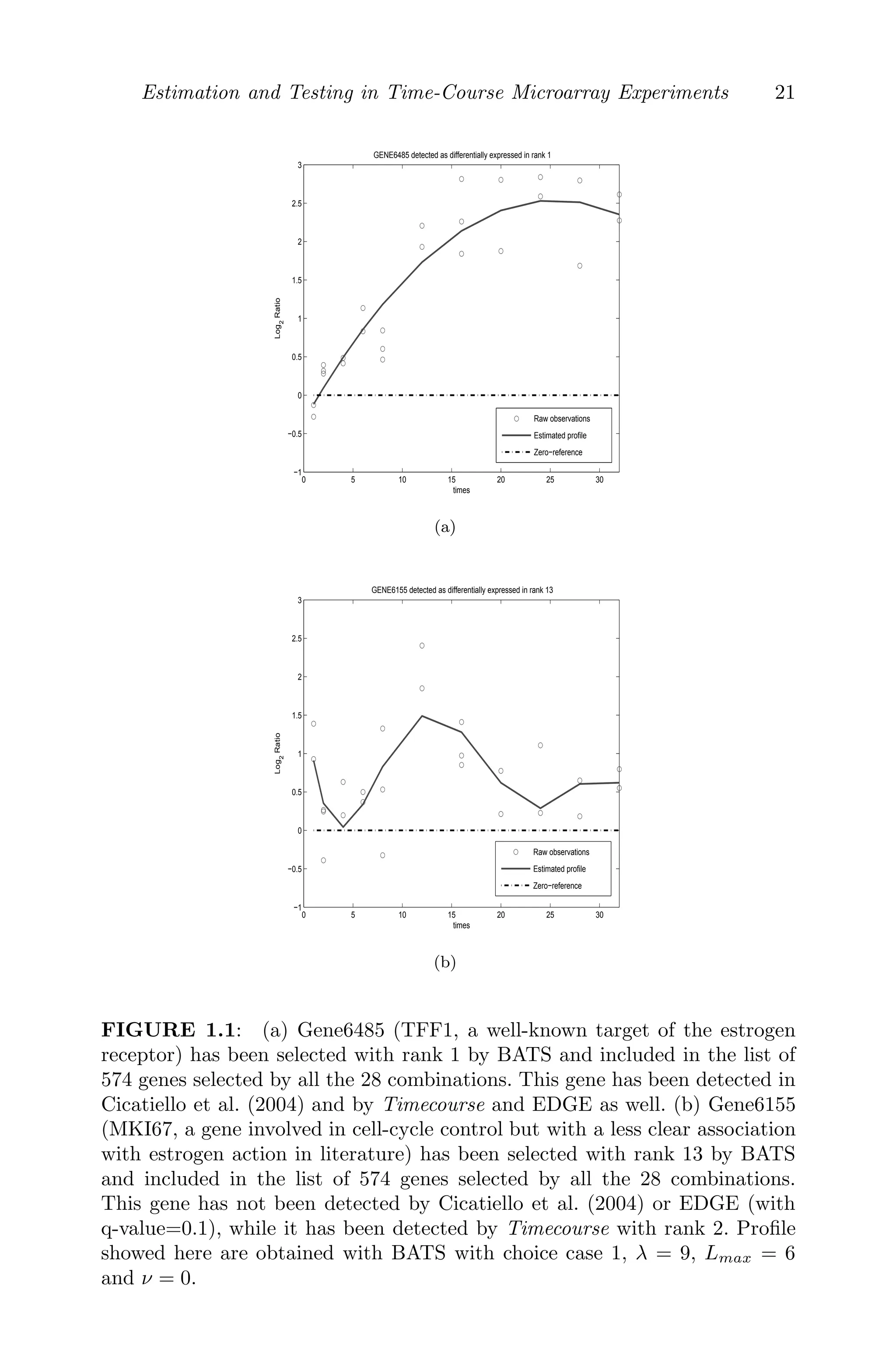
1.1Estimators of some gene expression profiles . . . . . . . . . . 21
2.1 Array effects as a function of expression level, for a wildtype
mouse expression data set of 3 arrays, as presented in Lewin
et al. (2006). Solid lines represent the spline array effects found
as part of the Bayesian model, dashed lines represent the loess
smoothed array effects. The histogram shows the distribution
of the observed gene expression levels. Differences between the
spline and loess curves are only apparent at low expression
levels, where there is very little data. . . . . . . . . . . . . . . 32
2.2 Left: sample variances and posterior mean variances (Inverse
Gamma prior) for the IRS2 mouse data (wildtype only). Right:
posterior mean variances from the Inverse Gamma and log Nor-
mal priors. . . . . . . . . . . . . . . . . . . . . . . . . . . . . . 33
2.3 Decision areas for 3 component mixture in the (P(zg = −1 |
y), P(zg = +1 | y)) space for different combination of penalty
ratios. All plots (apart from Bayes rule) have B = 0.4. . . . . 39
2.4 Posterior mean of δg under the mixture prior (y-axis) and under
the unstructured prior (x-axis) for IRS2 data. . . . . . . . . . 41
2.5 Volcano plots (ȳg, pg) based on different posterior probabilities
pg for IRS2 data (α = 0.05). In (d), 2 max(pg, 1 − pg) − 1 is
plotted for the corresponding posterior probability. . . . . . . 45
2.6 FDR estimates corresponding to 5 scenarios as labeled in Sec-
tion 2.3.1, plotted against the number of genes in the list (IRS2
data). . . . . . . . . . . . . . . . . . . . . . . . . . . . . . . . 46
2.7 False discovery (FDR) and non-discovery (FNR) rates for dif-
ferent thresholds, simulated data, as presented in Bochkina
Richardson (2007). Joint probability: light, minimum of pair-
wise probabilities: dark. . . . . . . . . . . . . . . . . . . . . . 49
2.8 Directed acyclic graph for the part of the model involved in pre-
dicting sum of squares data. Solid lines show the actual model
being fitted, while dotted lines show the predicted quantities. 52
2.9 Bayesian predictive p-values for checking the gene variance
prior, for two models applied to the IRS2 data (wildtype data
only). Left: exchangeable variances, right: equal variances. . . 53
xvii
23.
xviii
2.10 Directed acyclicgraph for predicting the data means. Solid lines
show the actual model being fitted, while dotted lines show the
predicted quantities. . . . . . . . . . . . . . . . . . . . . . . . 54
2.11 Bayesian mixed predictive p-values for checking separate mix-
ture components, for two models applied to the IRS2 data.
The three columns show histograms of the p-values for compo-
nents z = −1, 0, 1 separately. Each histogram uses only genes
allocated to that component with posterior probability greater
than 0.5. Top row shows results for the Gamma model in Equa-
tion 2.36, bottom row shows results for the Uniform model in
Equation 2.37. . . . . . . . . . . . . . . . . . . . . . . . . . . 56
3.1 The left panel shows the performance of the 11 gene classifier
of disease-free patients after at least 5 years versus patients
with metastases within 5 years. The horizontal lines represent
80% confidence intervals. The right panel shows the ROC curve
associated with this classifier. . . . . . . . . . . . . . . . . . . 79
3.2 The left panel shows the performance of the 8 gene classifier
for the 34 test samples in leukemia data. The horizontal lines
represent 80% confidence intervals. The right panel shows the
ROC curve associated with this classifier. . . . . . . . . . . . 80
3.3 Fitted prediction probabilities for the lymph node data. The
horizontal lines represent 80% confidence intervals. The right
panel shows the ROC curve associated with this classifier. . . 81
3.4 Fivefold cross-validation prediction probabilities for the lymph
node data. The horizontal lines represent 80% confidence in-
tervals. The right panel shows the ROC curve associated with
this classifier. . . . . . . . . . . . . . . . . . . . . . . . . . . . 82
3.5 Fitted prediction probabilities for the SNP data when regres-
sions with at most three variables are considered. The horizon-
tal lines represent 80% confidence intervals. The right panel
shows the ROC curve associated with this classifier. . . . . . 84
3.6 Two-fold cross-validation prediction probabilities for the SNP
data when regressions with at most three variables are consid-
ered. The horizontal lines represent 80% confidence intervals.
The right panel shows the ROC curve associated with this clas-
sifier. . . . . . . . . . . . . . . . . . . . . . . . . . . . . . . . . 86
4.1 Realizations from a Dirichlet process prior for different choices
of the DP precision parameter α. . . . . . . . . . . . . . . . . 103
5.1 Survival curve for breast cancer dataset. . . . . . . . . . . . . 127
5.2 Variance vs. mean relationship with model fit lines. . . . . . . 128
5.3 Trace plots of select parameters (σB, σm, and ρm) of measure-
ment error model with lag 1 autocorrelation. . . . . . . . . . 136
24.
xix
5.4 Scaled residualswith normal density curve. . . . . . . . . . . 139
5.5 Estimation of regression parameter with 95% HPD under mis-
specified error model. . . . . . . . . . . . . . . . . . . . . . . . 140
5.6 Estimation of latent expression under misspecified error model. 141
6.1 BRIDGE posterior probabilities . . . . . . . . . . . . . . . . . 156
7.1 Breast cancer specimen S0034 from Snijders et al. (2001) . . 167
7.2 Array CGH profiles of some pancreatic cancer specimens . . . 174
7.3 Array CGH profile of chromosome 13 of specimen GBM31 . . 176
7.4 Partial profile of chromosome 7 of specimen GBM29 . . . . . 177
7.5 Bayesian versus non-Bayesian approaches . . . . . . . . . . . 181
7.6 Simulated data set . . . . . . . . . . . . . . . . . . . . . . . . 182
7.7 Estimated means Ê[μj|Y ] for three independently generated
data sets (shown by solid, dashed, and dotted lines) plotted
against . . . . . . . . . . . . . . . . . . . . . . . . . . . . . . 183
8.1 Deep coalescence, with the contained gene tree (dashed line)
failing to coalesce in the ancestral population of species B and
C, leading to the allele sampled in B being more closely related
to allele in A, rather than the true sister species, C. . . . . . 205
8.2 Majority-rule consensus tree phylogeny of 178 species of true
frogs of the subfamily Raninae. Branches with posterior proba-
bility 0.9 are denoted by black dots at the descendant node.
Empty circles denote nodes on branches with posterior proba-
bility between 0.7 and 0.9. Stars indicate three species of frogs
endemic to the Indonesian island of Sulawesi. An arrow indi-
cates the only clade that was in the no-clock consensus tree but
not in the relaxed-clock consensus tree. . . . . . . . . . . . . . 216
8.3 Comparison of posterior probabilities of clades under the no-
clock and relaxed clock approaches, as estimated under 4 in-
dependent runs of 200 million generations each under each ap-
proach. . . . . . . . . . . . . . . . . . . . . . . . . . . . . . . . 217
10.1 ROC curves of the Bayesian methods. . . . . . . . . . . . . . 265
11.1 An example of Bayesian networks. . . . . . . . . . . . . . . . 272
11.2 Sample paths produced by SAMC and MH for the simulated
example. . . . . . . . . . . . . . . . . . . . . . . . . . . . . . . 282
11.3 The maximum a posteriori network structures learned by
SAMC and MH for the simulated example. . . . . . . . . . . 282
11.4 Progression paths of minimum energy values produced by
SAMC and MH for the simulated example. . . . . . . . . . . 284
11.5 Progression paths of minimum energy values produced by
SAMC and MH for the yeast cell cycle example. . . . . . . . 285
25.
xx
11.6 The maximuma posteriori Bayesian network learned by SAMC
for a subset of the yeast cell cycle data. . . . . . . . . . . . . 286
12.1 Scatter plot of estimated values λ∗
1,i in the ovarian cancer data
set (x-axis) against scores on the ovarian tumors of the lung and
breast cancer factors 1; these two sets of scores are constructed
by projection of the estimated factor loadings of lung and
breast factor 1 into the ovarian data set, as described in Section
12.2.3. . . . . . . . . . . . . . . . . . . . . . . . . . . . . . . . 303
12.2 A Venn diagram depicting intersections of the gene lists of fac-
tor 1 from breast, lung, and ovarian cancers (total number of
genes in each factor listed outside the circles, the number of
genes in each intersection listed inside). Although the ovarian
cancer factor 1 involves a significantly smaller number of genes
than the other cancers, almost all of these (109 of 124) are
common with those in the lung and breast factors. . . . . . . 304
12.3 Patterns of expression of the 109 genes in the intersection group
in Figure 12.2. The genes are ordered the same in the three
heat-map images, and the patterns of expression across samples
are evidently preserved across genes in this set. . . . . . . . . 305
12.4 Factors 4 and 5 from the E2F3 signature factor profile in the
lung cancer data set show a clear ability to distinguish between
adenocarcinoma and squamous cell carcinoma. The figure dis-
plays probabilities of squamous versus adenocarcinoma from
binary regression models identified using SSS. . . . . . . . . . 306
12.5 Patterns of expression of the genes in factor 4 in lung can-
cer. This factor shows differential expression of 350 genes that
distinguish between squamous cell carcinoma and adenocarci-
noma. It is therefore appropriate that the pattern of expression
is clearly not conserved in the ovarian and breast cancers. . . 307
12.6 Kaplan–Meyer curves representing survival in breast cancer pa-
tients with above/below median scores for the E2F/NF-Y fac-
tor. Suppression of the E2F/NF-Y pathway appears to be as-
sociated with the decreased probability of long-term survival. 308
12.7 Kaplan–Meyer curves representing survival in ovarian cancer
patients with above/below median scores for the E2F/TFDP2
factor. Suppression of the E2F/TFDP2 pathway appears to be
associated with decreased probability of long-term survival. . 309
12.8 Kaplan–Meyer curves representing survival in lung cancer pa-
tients with above/below median scores for the E2F/ELF1 fac-
tor. Suppression of the E2F/ELF1 pathway appears to be as-
sociated with decreased probability of long-term survival. . . 310
12.9 This flowchart shows the overall strategy for analyzing micro-
array expression data. . . . . . . . . . . . . . . . . . . . . . . 311
26.
xxi
13.1 Estimated survivalfunction for breast carcinomas data using
RVM model. . . . . . . . . . . . . . . . . . . . . . . . . . . . 332
13.2 Estimated survival function for breast carcinomas data using
SVM model. . . . . . . . . . . . . . . . . . . . . . . . . . . . . 333
13.3 Estimated survival function for DLBCL data using RVM
model. . . . . . . . . . . . . . . . . . . . . . . . . . . . . . . . 334
13.4 Estimated survival function for DLBCL data using SVM
model. . . . . . . . . . . . . . . . . . . . . . . . . . . . . . . . 335
14.1 Raw data. The left panel shows the recorded spectra for normal
samples. The right panel shows the spectra for tumor samples.
The X axis are the m/z values. . . . . . . . . . . . . . . . . . 346
14.2 p(J | Y ) and p(Jk | Y ). The histogram in the left panel shows
the posterior probabilities for the number of distinct peaks. We
find the posterior mode around 18 peaks. The boxplots (right
panel) summarize the posterior distributions p(Jk | Y ). The
number of terms in the baseline mixtures was constrained at
Jk ≤ 5. . . . . . . . . . . . . . . . . . . . . . . . . . . . . . . 355
14.3 E[fk(m) | Y, xk = x]. Estimated spectrum for normal and tu-
mor samples. . . . . . . . . . . . . . . . . . . . . . . . . . . . 356
14.4 Posterior inference defines a probability model on the unknown
spectra. The two panels show ten draws from p(fk | Y ) for
xk = 0 (left) and xk = 1 (right). . . . . . . . . . . . . . . . . . 356
14.5 E(1 − λj | Y ). Posterior expected probability of differential
expression for the reported peaks. . . . . . . . . . . . . . . . . 357
14.6 Detected proteins. The figure plots the posterior estimated
weights E(wxj | Y ) against mass/charge ratios E(j | Y ). Panel
(a) plots the average weight E(wxj | Y ), averaging over all it-
erations that reported a protein peak at j. Panel (b) scales
the average weight by the probability of a peak being detected
at j (i.e., no detection is counted as w = 0). For genes with
E(λj | Y ) 0.5 we plot the posterior expectation of w0j. For
differentially expressed genes we plot posterior expectations for
wxj for both conditions, x = 0, 1, linked with a line segment.
Only proteins with posterior expected weight greater or equal
to 0.05 are shown. . . . . . . . . . . . . . . . . . . . . . . . . 357
14.7 Proteins included in a panel of biomarkers to classify samples
according to biologic condition x. Let ER = {1, . . . , R} denote
the locations of peaks, i.e., proteins, included in a subset of size
R. The figure plots for each location r the minimum size R of
subsets that include r. . . . . . . . . . . . . . . . . . . . . . 358
14.8 Some aspects of the MCMC simulation. The left panel plots
the imputed number of proteins J against iteration. The right
panel plots the locations j of the imputed beta kernels (x-axis)
over iterations (y-axis). . . . . . . . . . . . . . . . . . . . . . 358
27.
xxii
15.1 Plots ofmedians and inter quartile ranges (IQR) of 10,000
Bayes factors with the variance σ2
of each gene ranging from
0.5 to 10. . . . . . . . . . . . . . . . . . . . . . . . . . . . . . 374
15.2 Densities of gene expressions for selected genes. . . . . . . . . 384
16.1 Image analysis of microarray experiment. Each probe will pro-
vide at least four readings: a pair of statistics Rf and Rb indi-
cating the feature and background intensities in the red chan-
nel, and a pair of summary statistics Gf and Gb indicating
the feature and background intensities in the green channel,
respectively. . . . . . . . . . . . . . . . . . . . . . . . . . . . . 396
28.
Preface
Recent advances ingenome sequencing (genomics) and protein identification
(proteomics) have given rise to challenging research problems that require
combined expertise from statistics, biology, computer science, and other fields.
Similar challenges arise dealing with modeling genetic data in the form of se-
quences of various types, e.g., SNIP, RAPD, and microsatellite data. The in-
terdisciplinary nature of bioinformatics presents many research challenges re-
lated to integrating concepts, methods, software, and multi-platform data. In
addition to new tools for investigating biological systems via high-throughput
genomic and proteomic measurements, statisticians face many novel method-
ological research questions generated by such data. The work in this volume
is dedicated to the development and application of Bayesian statistical meth-
ods in the analysis of high-throughput bioinformatics data that arise from
problems in medical research, in particular cancer and other disease related
research, molecular and structural biology.
This volume does not aim to be comprehensive in all areas of bioinformat-
ics. Rather, it presents a broad overview of statistical inference, clustering,
and classification problems related to two main high-throughput platforms:
microarray gene expression and phylogenic analysis. The volume’s main fo-
cus is on the design, statistical inference, and data analysis, from a Bayesian
perspective, of data sets arising from such high-throughput experiments. All
the chapters included in the volume focus on Bayesian methodologies, para-
metric as well as nonparametric, but each is self contained and independent.
There are topics closely related to each other, but we feel there is no need
to maintain any kind of sequencing for reading the chapters. The chapters
have been arranged purely in alphabetical order according to the last name
of the first author and, in no way, should it be taken to mean any preferential
order. Chapter 1 provides estimation and testing in time-course microarray
experiments. This chapter discusses a variety of recently developed Bayesian
techniques for detection of differentially expressed genes on the basis of time
series of microarray data. Chapter 2 considers classification for differential
gene expression using hierarchical Bayesian models. Chapter 3 deals with ap-
plications of mode-oriented stochastic search algorithms for discrete multi-way
data for genome wide studies. Chapter 4 develops novel Bayesian nonparamet-
ric approaches to bioinformatics problems. Dirichlet process mixture models
are introduced for multiple testing, high-dimensional regression, clustering,
and functional data analysis. Chapter 5 develops measurement error and sur-
vival models for cDNA microarrays. Chapter 6 focuses on robust Bayesian
xxiii
29.
xxiv
inference for differentialgene expression. Chapter 7 develops Bayesian hid-
den Markov modeling approach for CGH array data. Bayesian approaches
to phylogenic analysis are developed in Chapter 8. Chapter 9 is concerned
with gene selection for identification of biomarkers in high-throughput data.
Chapter 10 develops sparsity priors for protein–protein interaction predic-
tions. Chapter 11 describes Bayesian networks learning for gene expression
data. Chapter 12 describes in-vitro to in-vivo factor profiling in genomic ex-
pressions. Proportional hazards regression using Bayesian kernel machines is
considered in Chapter 13. Chapter 14 focuses on a Bayesian mixture model for
protein biomarker discovery using matrix-assisted laser desorption and ioniza-
tion mass spectrometry. Chapter 15 focuses on general Bayesian methodology
for detecting differentially expressed genes. Bayes and empirical Bayes meth-
ods for spotted microarray data analysis are considered in Chapter 16. Finally
Chapter 17 focuses on the Bayesian classification method for QTL mapping.
We thank all the collaborators for contributing their ideas and insights to-
ward this volume in a timely manner. We fail in our duties if we do not express
our sincere indebtedness to our referees, who were quite critical and unbiased
in giving their opinions. We do realize that despite of their busy schedules
the referees offered us every support in commenting on various chapters. Un-
doubtedly, it is the joint endeavor of the contributors and the referees that
emerged in the form of such an important and significant volume for the
Bayesian world.
We thankfully acknowledge David Grubbs from Chapman Hall, CRC, for
his continuous encouragement and support of this project. Our special thanks
go to our spouses, Rita, Amrita, and Mou, for their continuous support and
encouragement.
We are excited by the continuing opportunities for statistical challenges in
the area of bioinformatics data analysis and modeling from a Bayesian point
of view. We hope our readers will join us in being engaged with changing
technologies and statistical development in this area of bioinformatics.
Dipak K. Dey
Samiran Ghosh
Bani Mallick
MATLAB R
is a registered trademark of The Math Works, Inc. For product
information, please contact:
The Math Works
3 Apple Hill Drive
Natick, MA
Tel: 508-647-7000
Fax: 508-647-7001
Email: info@mathworks.com
Web: http://www.mathworks.com
30.
Symbol Description
σ2
Variance ofthe instrumen-
tal error.
N Number of genes in a mi-
croarray.
M Total number of array in an
experiment.
n Number of different time
points in the temporal in-
terval of the experiment.
K Maximum number of repli-
cates in a time points of the
experiment.
zi The vector of measure-
ments for the i-th gene.
si(t) Underlying function of the
i-th gene expression profile.
H Number of samples in the
experiments.
xxv
32.
Chapter 1
Estimation andTesting in
Time-Course Microarray
Experiments
C. Angelini, D. De Canditiis, and M. Pensky
(I.A.C.) CNR, Italy, and University of Central Florida, USA
1.1 Abstract ................................................................. 1
1.2 Introduction ............................................................. 2
1.3 Data Structure ........................................................... 3
1.4 Statistical Methods for the One-Sample Microarray Experiments ...... 6
1.5 Statistical Methods for the Multi-Sample Microarray Experiments .... 11
1.6 Software .................................................................. 16
1.7 Comparisons between Techniques ....................................... 19
1.8 Discussion ................................................................ 20
Acknowledgments ........................................................ 22
1.1 Abstract
The paper discusses a variety of recently developed Bayesian techniques for
detection of differentially expressed genes on the basis of time series microar-
ray data. These techniques have different strengths and weaknesses and are
constructed for different kinds of experimental designs. However, the Bayesian
formulations, which the above described methodologies utilize, allow one to
explicitly use prior information that biologists may provide. The methods
successfully deal with various technical difficulties that arise in microarray
time-course experiments such as a large number of genes, a small number of
observations, non-uniform sampling intervals, missing or multiple data, and
temporal dependence between observations for each gene.
Several software packages that implement methodologies discussed in the
paper are described, and limited comparison between the techniques using a
real data example is provided.
1
33.
2 Bayesian Modelingin Bioinformatics
1.2 Introduction
Gene expression levels in a given cell can be influenced by different fac-
tors, namely pharmacological or medical treatments. The response to a given
stimulus is usually different for different genes and may depend on time. One
of the goals of modern molecular biology is the high-throughput identifica-
tion of genes associated with a particular treatment or biological process of
interest. The recently developed technology of microarrays allows one to si-
multaneously monitor the expression levels of thousands of genes. Although
microarray experiments can be designed to study different factors of interest,
in this paper, for simplicity, we consider experiments involving comparisons
between two biological conditions (for example, “control” and “treatment”)
made over the course of time.
The data may consist of measurements of the expression levels of N genes
in two distinct independently collected samples made over time [0,T] (the,
so called,“two-sample problem”), or measurements of differences in the ex-
pression levels between the two samples (the “one-sample problem”). In both
cases, the objective is first to identify the genes that are differentially ex-
pressed between the two biological samples and then to estimate the type of
response. Subsequently, the curves may undergo some kind of clustering in
order to group genes on the basis of their type of response to the treatment.
The problem represents a significant challenge since the number of genes
N is very large, while the number of time points n where the measurements
are made is rather small and, hence, no asymptotic method can be used. The
data is contaminated by usually non-Gaussian heavy-tailed noise. In addi-
tion, non-uniform sampling intervals and missing or multiple data makes time
series microarray experiments unsuitable to classical time-series and signal
processing algorithms.
In the last decades the statistical literature has mostly addressed static mi-
croarray experiments, see Efron et al. (2001), Lonnstedt and Speed (2002),
Dudoit et al. (2002), Kerr et al. (2000), Ishwaran and Rao (2003), among
many others. The analysis of time-course microarray was mainly carried out by
adapting some existing methodologies. For example, SAM version 3.0 software
package—originally proposed by Tusher et al. (2001) and later described in
Storey et al. (2003a, 2003b)—was adapted to handle time-course data by con-
sidering the time points as different groups. In a similar manner, the ANOVA
approach by Kerr et al. (2000) and Wu et al. (2003) was applied to time-course
experiments by treating the time variable as a particular experimental factor.
Similar approaches have been considered by Di Camillo et al. (2005) and the
Limma package by Smyth (2005), while the paper of Park et al. (2003) uses
linear model regression combined with ANOVA analysis. All these methods
can be useful when very short time-course experiments have to be analyzed
(3-4 time points), however they have the shortcoming of applying statistical
34.
Estimation and Testingin Time-Course Microarray Experiments 3
techniques designed for static data to time-course data, so that the results
are invariant under permutation of the time points. The biological temporal
structure of data is ignored.
Although microarray technology has been developed quite recently, nowa-
days, time-course experiments are becoming increasingly popular: a decreasing
cost of manufacturing allows larger number of time points, moreover, it is well
recognized that the time variable plays a crucial role in the development of a
biological process. Indeed, Ernst and Bar-Joseph (2006) noted that currently
time-course microarray experiments constitute about 30% of all microarray
experiments (including both cell cycle and drug response studies). Neverthe-
less, there is still a shortage of statistical methods that are specifically designed
for time-course microarray experiments.
This realization led to new developments in the area of analysis of time-
course microarray data, see de Hoon et al. (2002), Bar-Joseph et al. (2003a,
2003b), and Bar-Joseph (2004). More recently, Storey et al. (2005), Conesa
et al. (2006), Hong and Li (2006), and Angelini et al. (2007, 2009) proposed
functional data approaches where gene expression profiles are expanded over
a set of basis functions and are represented by the vectors of their coeffi-
cients thereafter. Tai and Speed (2006, 2007) considered a multivariate empir-
ical Bayes approach, which applies statistical inference directly to the phys-
ical data itself. Another important class of methods which is based on the
hidden Markov model approaches, was pioneered by Yuan and Kendziorski
(2006).
The goal of the present chapter is to review the more recent techniques for
analysis of the time-course microarray data, as well as the software designed
for implementing them. The rest of the paper is organized as follows. Section
1.3 describes various possible designs of time-series microarray experiment
with particular focus on the one-sample and the two-sample (or multi-sample)
designs. Section 1.4 reviews the methods that are constructed specifically for
the one-sample setup, while Section 1.5 is devoted to the methods for the
two-sample and the multi-sample setups. Section 1.6 provides information
on several software packages that implement methodologies described above.
Section 1.7 reports results of the application of some recent techniques to a
real data set. Finally, Section 1.8 concludes the chapter with a discussion.
1.3 Data Structure
The goal of the present paper is to review statistical methods for the au-
tomatic detection of differentially expressed genes in time series microarray
experiments. However, the choice of the statistical methodology used for the
analysis of a particular data set strongly depends on the way in which the data
35.
4 Bayesian Modelingin Bioinformatics
have been collected since different experimental designs account for different
biological information and different assumptions.
First, one needs to distinguish longitudinal studies from independent and
factorial ones. Pure longitudinal data is obtained when the same sample is
monitored over a period of time, and different samples are separately and
distinguishably recorded in the course of the experiment. Independent (or
cross-sectional) experimental design takes place when at each time point inde-
pendent samples are recorded, and replicates are indistinguishable from each
other. Finally, factorial designs are those where two or more experimental
factors are involved in the study. Also, one needs to distinguish between tech-
nical replicates and biological replicates, since the latter introduce additional
variation in the data.
The choice of a statistical technique for data analysis is influenced by the
number of time points at which observations are available (usually, 6 or more
time points, or 3–5 time points for a “short” time series) and the grid design
(equispaced or irregular). The presence of missing data also affects the choice
of statistical methodology.
The objective of microarray experiments is to detect the differences in gene
expression profiles in the biological samples taken under two or more ex-
perimental conditions. The differences between gene expression levels can be
measured directly (usually, in logarithmic scale) leading to a “one-sample”
problem where the differences between profiles are compared to an identi-
cal zero curve. If the measurements on each sample are taken independently,
then one has a “two-sample” or a “multi-sample” problem where the goal is
to compare the gene expression profiles for different samples. For example, if
an experiment consists of a series of two-color microarrays, where the control
(untreated) sample is directly hybridized with treated samples after various
time intervals upon treatment, then one has the one-sample problem. On the
other hand, if the two samples are hybridized on one-color arrays or indepen-
dently hybridized with a reference on two color arrays, then it leads to the
two-sample problem.
In what follows, we review statistical methods for the one-sample, two-
sample, and multi-sample problems commenting on what types of experimen-
tal designs are accommodated by a particular statistical technique and how it
deals with an issue of irregular design and missing data. However, regardless
the type of experimental design, the microarray data are assumed to be al-
ready pre-processed to remove systematic sources of variation. For a detailed
discussion of the normalization procedures for microarray data we refer the
reader to, e.g., Yang et al. (2002), Cui et al. (2002), McLachlan et al. (2004),
or Wit and McClure (2004).
1.3.1 Data Structure in the One-Sample Case
In general, the problem can be formulated as follows. Consider microar-
ray data consisting of the records of N genes. The records are taken at n
36.
Estimation and Testingin Time-Course Microarray Experiments 5
different time points in [0, T ] where the sampling grid t(1)
, t(2)
, . . . , t(n)
is not
necessarily uniformly spaced. For each array, the measurements consist of N
normalized log2-ratios zj,k
i , where i = 1, . . . , N, is the gene number, index j
corresponds to the time point t(j)
and k = 1, . . . , k
(j)
i , k
(j)
i ≥ 0, accommodates
for possible technical or biological replicates at time t(j)
. Note that usually,
by the structure of the experimental design, k
(j)
i are independent of i, i.e.,
k
(j)
i ≡ k(j)
with M =
n
j=1 k(j)
being the total number of records. However,
since some observations may be missing due to technical errors in the experi-
ment, we let k
(j)
i to depend on i so that the total number of records for gene
i is
Mi =
n
j=1
k
(j)
i . (1.1)
The number of time points is relatively small (n ≈ 10) and very few replica-
tions are available at each time point (k
(j)
i = 0, 1, . . . K where K = 1, 2, or
3) while the number of genes is very large (N ≈ 10, 000).
1.3.2 Data Structure in the Multi-Sample Case
Consider data consisting of measurements of the expression levels of N
genes in two or more distinct independently collected samples made over time
[0,T].
We note that, when the number of samples is two, the objective is first to
identify the genes that are differentially expressed between the two samples
and then to estimate the type of response. On the other hand, when more
samples are considered one may be interested in detecting both genes that are
differentially expressed under at least one biological condition or some specific
contrasts, in a spirit that is similar to the multi-way ANOVA model and then
to estimate the type of effect. In general, the problem can be formulated
as follows. For sample ℵ, ℵ = 1, · · · , H, data consists of the records zj,k
ℵi , i =
1, · · · , N, on N genes, which are taken at time points t
(j)
ℵ ∈ [0, T ], j = 1, .., nℵ.
For gene i at a time point t
(j)
ℵ , there are k
(j)
ℵi (with k
(j)
ℵi = 0, 1, . . ., K) records
available, making the total number of records for gene i in sample ℵ to be
Mℵi =
n
j=1
k
(j)
ℵi . (1.2)
Note that in this general setup it is required neither that the observations
for the H samples are made at the same time points nor that the number
of observations for different samples is the same. This model can be applied
when observations on the H samples are made completely separately: the only
requirement is that the samples are observed over the same period of time.
The orders of magnitude of N, n, and K are the same as in the one-sample
case.
37.
6 Bayesian Modelingin Bioinformatics
1.4 Statistical Methods for the One-Sample Microarray
Experiments
In this section we present the more recent and important methods for the
one-sample microarray time-course experiments.
1.4.1 Multivariate Bayes Methodology
Tai and Speed (2006) suggest multivariate Bayes methodology for identifi-
cation of differentially expressed genes. Their approach is specifically designed
for longitudinal experiments where each replicate refers to one individual. The
technique requires that for each gene the number of replicates k
(j)
i is constant
for all time points k
(j)
i = ki, so that for each gene i there are ki independent
n-dimensional observations zi,k = (z1,k
i , . . . , zn,k
i )T
∈ Rn
, k = 1, . . . , ki. Each
vector is modeled using multivariate normal distribution zi,k ∼ Nn(Iiμi, Σi)
where Ii is the Bernoulli random variable, which is equal to 1 when gene i
is differentially expressed and zero otherwise. For each gene i, the following
hierarchical Bayesian model is built:
μi|Σi, Ii = 1 ∼ N(0, η−1
i Σi)
μi|Σi, Ii = 0 = 0
Σi ∼ InverseWishart(νi, νiΛ−1
i )
P(Ii = 0) = π0.
Here νi, ηi and Λi are gene-specific parameters to be estimated from the
data, while π0 is a global user-defined parameter. To test whether a gene is
differentially expressed, Tai and Speed (2006) evaluate posterior odds of Ii = 1
Oi =
P(Ii = 1|zi,1, · · · , zi,ki )
P(Ii = 0|zi,1, · · · , zi,ki )
. (1.3)
Denote by z̄i and Si the mean and the sample covariance matrix of the vectors
zi,1, · · · , zi,ki , and let
S̃i = [(ki − 1)Si + νiΛi]/(ki − 1 + νi) and t̃i =
kiS̃
−1/2
i ¯
zi
be the moderated sample covariance matrix and multivariate t-statistic. Then,
posterior odds (1.3) can be rewritten as
1 − π0
π0
ηi
ηi + ki
n/2
ki − 1 + νi + t̃T
i t̃i
ki − 1 + νi + (ki + ηi)−1ηt̃T
i t̃i
(ki+νi)/2
. (1.4)
Unknown gene specific parameters νi, ηi and Λi are estimated using a ver-
sion of empirical Bayes approach described in Smyth (2004) and are plugged
38.
Estimation and Testingin Time-Course Microarray Experiments 7
into expressions (1.4). After that, genes are ordered according to the values
of posterior odds (1.4), and genes with the higher values of Oi are consid-
ered to be differentially expressed. Note that the user-defined parameter π0
does not modify the order in the list of differentially expressed genes. The au-
thors do not define the cut off point, so the number of differentially expressed
genes has to be chosen by a biologist. Tai and Speed (2006) also notice that
when all genes have the same number of replicates ki = k, then the posterior
odds is a monotonically increasing function of T̃2
i = t̃T
i t̃i. Therefore, in this
case they suggest to use the T̃2
i , i = 1, · · · , N, statistics instead of posterior
odds since they do not require estimation of ηi and lead to the same ranking
as (1.4).
Since Tai and Speed (2006) apply Bayesian techniques directly to the vectors
of observations, the method is not flexible. The analysis can be carried out
only if the same number of replicates is present at every time point. If any
observation is absent, missing data techniques have to be applied. Moreover,
the results of analysis are completely independent of the time measurements,
so that it is preferable to apply the technique only when the grid is equispaced.
Finally, Tai and Speed (2006) do not provide estimators of the gene expression
profiles.
1.4.2 Functional Data Approach
Although approach of Storey et al. (2005) is not Bayesian, we present it
here since it is the first functional data approach to the time-series microar-
ray data. Storey et al. (2005) treat each record zj,k
i as a noisy measurement
of a function si(t) at a time point t(j)
. The objective of the analysis is to
identify and estimate the curves si(t) that are different from the identical
zero.
Since the response curve for each gene is relatively simple and only a few
measurements for each gene are available, Storey et al. (2005) estimate each
curve si(t) by expanding it over a polynomial or a B-spline basis
si(t) =
Li
l=0
c
(l)
i φl(t). (1.5)
The number of the basis functions is assumed to be the same for each gene:
Li = L, i = 1, · · · , N. Therefore, each function is described by its (L + 1)
dimensional vector of coefficients ci. The hypotheses to be tested are therefore
of the form H0i : ci ≡ 0 versus H1i : ci ≡ 0.
The vector of coefficients is estimated using the penalized least squares
algorithm. In order to choose the dimension of the expansion (1.5), Storey
et al. (2005) apply “eigen-gene” technique suggested by Alter et al. (2000).
The basic idea of the approach is to take a singular value decomposition
of the data and extract the top few “eigen-genes,” which are vectors in the
gene space. For those genes the number of basis functions is determined by
39.
8 Bayesian Modelingin Bioinformatics
generalized cross-validation. After that, this estimated value of L is used to fit
the curves for all genes under investigation. The statistic for testing whether
gene i is differentially expressed is analogous to the t or F statistics, which
are commonly used in the static differential expression case:
Fi = (SS0
i − SS1
i )/SS1
i
where SS0
i is the sum of squares of the residuals obtained from the model
fit under the null hypothesis, and SS1
i is the analogous quantity under the
alternative hypothesis. The larger Fi is, the better the alternative model fit
is over the null model fit. Therefore, it is reasonable to rank all the genes
by the size of Fi, i.e., gene i is considered to be differentially expressed if
Fi ≥ c for some cutoff point c. Since non-Gaussian heavy-tailed errors are
very common for microarray data, the distribution of statistics Fi under the
null hypothesis is assumed to be unknown. For this reason, the p-value for
each gene is calculated using bootstrap resampling technique as the frequency
by which the null statistics exceed the observed statistic.
However, although the p-value is a useful measure of significance for testing
an individual hypothesis, it is difficult to interpret a p-value when thousands
of hypotheses H0i, i = 1, · · · , N, are tested simultaneously. For this reason,
the authors estimate q-values, which are the false discovery rate (FDR) related
measure of significance. The q-values are evaluated on the basis of the p-values
using an algorithm described in Storey and Tibshirani (2003a).
The approach of Storey et al. (2005) is very flexible: no parametric as-
sumptions are made about distributions of the errors, moreover, methodology
allows to take into account variations between individuals. However, this flex-
ibility comes at a price: the technique requires resampling methods, which
may be rather formidable to a practitioner.
1.4.3 Empirical Bayes Functional Data Approach
Angelini et al. (2007) propose an empirical Bayes functional data approach
to identification of the differentially expressed genes, which is a good com-
promise between a rather inflexible method of Tai and Speed (2006) and a
computationally expensive technique of Storey et al. (2005).
Similarly to Storey et al. (2005), in Angelini et al. (2007) each curve si(t)
is expanded over an orthonormal basis (Legendre polynomials or Fourier) as
in (1.5) and is characterized by the vector of its coefficients ci, although the
lengths (Li + 1) of the vectors may be different for different genes.
The genes are assumed to be conditionally independent, so that for each i,
i = 1, . . . , N the data is modeled as
zi = Dici + ζi (1.6)
40.
Estimation and Testingin Time-Course Microarray Experiments 9
where zi = (z1,1
i . . . z
1,k
(1)
i
i , · · · , zn,1
i , . . . z
n,k
(n)
i
i )T
∈ RMi
is the column vec-
tor of all measurements for gene i (see (1.1)), ci = (c0
i , . . . , cLi
i )T
∈
RLi+1
is the column vector of the coefficients of si(t) in the chosen basis,
ζi = (ζ1,1
i , . . . , ζ
1,k
(1)
i
i , · · · , ζn,1
i , . . . , ζ
n,k
(n)
i
i )T
∈ RMi
is the column vector of
random errors and Di is the Mi × (Li + 1) block design matrix the j-row of
which is the block vector [φ0(t(j)
) φ1(t(j)
) . . . φLi (t(j)
)] replicated k
(j)
i times.
The following Bayesian model is imposed on the data:
zi | Li, ci, σ2
∼ N(Dici, σ2
IMi );
Li ∼ Pois∗
(λ, Lmax), Poisson with parameter λ truncated at Lmax ;
ci | Li, σ2
∼ π0δ(0, . . . , 0) + (1 − π0)N(0, σ2
τ2
i Q−1
i ).
Here, π0 is the prior probability that gene i is not differentially expressed.
Matrix Qi is a diagonal matrix that accounts for the decay of the coefficients
in the chosen basis and depends on i only through its dimension.
Parameter σ2
is also assumed to be a random variable σ2
∼ ρ(σ2
), which
allows to accommodate possibly non-Gaussian errors (quite common in mi-
croarray experiments), without sacrificing closed form expressions for estima-
tors and test statistics. In particular, the following three types of priors ρ(·)
are considered:
case 1: ρ(σ2
) = δ(σ2
− σ2
0), the point mass at σ2
0. The marginal distribution
of the error is normal.
case 2: ρ(σ2
) = IG(γ, b), the Inverse Gamma distribution. The marginal
distribution of the error is Student T .
case 3: ρ(σ2
) = cμσ(M−1)
e−σ2
μ/2
, where M is the total number of arrays
available in the experimental design setup. If the gene has no missing
data (Mi = M), i.e. all replications at each time point are available,
then the marginal distribution of the error is double exponential.
The procedure proposed in Angelini et al. (2007) is carried out as follows.
The global parameters ν, λ and
Lmax are defined by a user. The global pa-
rameters π0 and case-specific parameters, σ2
0 for case 1, γ and b for case 2,
and μ for case 3 are estimated from the data using records on all the genes
that have no missing values. The gene-specific parameter τ2
i is estimated by
maximizing the marginal likelihood p(zi) while Li is estimated using the mode
or the mean of the posterior pdf p(Li|zi).
In order to test the hypotheses H0i : ci ≡ 0 versus H1i : ci ≡ 0 for
i = 1, . . . , N, and estimate the gene expression profiles, Angelini et al. (2007)
introduce, respectively, the conditional and the averaged Bayes factors
BFi(L̂i) =
(1 − π0)P(H0i|zi, L̂i)
π0P(H10i|zi, L̂i)
, BFi =
(1 − π0)P(H0i|zi)
π0P(H10i|zi)
.
41.
10 Bayesian Modelingin Bioinformatics
Bayes factors can be evaluated explicitly using the following expressions
BFi(L̂i) = A0i(L̂i)/A1i(L̂i), BFi =
Lmax
Li=0
gλ(Li)A0i(Li)
(1.7)
×
Lmax
Li=0
gλ(Li)A1i(Li)
(1.8)
where
A0i(Li) = F(Mi, zT
i zi), A1i(Li)
= τ
−(Li+1)
i [(Li + 1)!]ν
|Vi|−1/2
F(Mi, Hi(zi)),
Vi = DT
i Di + τ−2
i Qi, Hi(zi) = zT
i zi − zT
i DiV−1
i DT
i zi,
and
F (A, B) =
⎧
⎪
⎪
⎪
⎨
⎪
⎪
⎪
⎩
σ−2A
0 e−B/2σ2
0 in case 1,
Γ(A+γ)
Γ(γ) b−A
(1 + B
2b )−(A+γ)
in case 2,
B(M+1−2A)/4
μ(M+1+2A)/4
2(M−1)/2 Γ((M+1)/2)
K((M+1−2A)/2)(
√
Bμ) in case 3,
Here Kh(·) is the Bessel function of degree h (see Gradshteyn and
Ryzhik [1980] for the definition and Angelini et al. [2007]) for additional de-
tails).
The authors note that the two Bayes factors defined in (1.7) lead to an al-
most identical list of selected genes with the selection on the basis of BFi being
more theoretically sound but also slightly more computationally expensive.
Bayes factors BFi, although useful for independent testing of the null hy-
potheses H0i, i = 1, . . . , N, do not account for the multiplicity when test-
ing a large number of hypotheses simultaneously. In order to take into ac-
count multiplicity, the authors apply a Bayesian multiple testing procedure of
Abramovich and Angelini (2006).
Finally, the coefficients ci for the differentially expressed genes are estimated
by the posterior means
ĉi =
(1 − π0)/π0
BFi(L̂i) + (1 − π0)/π0
DT
i Di + τ̂−2
i Qi
−1
DT
i zi.
Methodology of Angelini et al. (2007) is much more computationally effi-
cient than that of Storey et al. (2005): all Bayesian calculations use explicit
formulae and, hence, are easy to implement. In addition, by allowing a different
number of basis functions for each curve, it avoids the need to pre-determine
the group of the most significant genes in order to select the dimension of
42.
Estimation and Testingin Time-Course Microarray Experiments 11
the fit. Also, by using hierarchical Bayes procedure for multiplicity control,
Angelini et al. (2007) avoid a somewhat ad-hoc evaluation of the p-values.
On the other hand, the algorithm of Angelini et al. (2007) is much more
flexible than that of Tai and Speed (2006): it takes into account the time
measurements allowing not necessarily equispaced time point and different
number of replicates per time point. It also avoids tiresome missing data
techniques and both ranks the genes and provides a cutoff point to determine
which genes are differentially expressed. However, we note that in Angelini et
al. (2007) the replicates are considered to be statistically indistinguishable, so
that the method cannot take advantage of a longitudinal experimental design.
1.5 Statistical Methods for the Multi-Sample Microar-
ray Experiments
Many of the procedures suggested in literature are specifically constructed
for the two-sample or multi-sample design, or can be easily adapted to it.
For example, the functional data approach of Conesa et al. (2006) is directly
applicable to the multi-sample design and Storey et al. (2005) accommodates
the two-sample design, requiring some changes for the extension to the multi-
sample design.
1.5.1 Multivariate Bayes Methodology in the Two-Sample
Case
Tai and Speed (2006) reduce the two-sample case to the one-sample case
by assuming that the number of time points in both samples is the same,
and also that the number of replications for each time point is constant, i.e.,
n1 = n2 = n and k
(j)
ℵi = kℵi, ℵ = 1, 2. It is also supposed implicitly that
time measurements are the same on both samples, i.e., t
(j)
1 = t
(j)
2 , j = 1, .., n.
Under these restrictions, Tai and Speed (2006) model the k-th time series for
gene i in sample ℵ as zℵ
i,k ∼ N(μℵi, Σi), ℵ = 1, 2. The prior imposed on the
vector μi = μ2i − μ1i is identical to the prior in the Section 1.4.1, and the
results of the analysis are very similar too. This model does not easily adapt
to a general multi-sample setup.
1.5.2 Estimation and Testing in Empirical Bayes Functional
Data Model
Angelini et al. (2009) propose an extension of the empirical Bayes functional
data procedure of Section 1.4.3 to the case of the two-sample and multi-sample
experimental design. For a gene i in the sample ℵ, it is assumed that evolution
43.
12 Bayesian Modelingin Bioinformatics
in time of its expression level is governed by a function sℵi(t) and each of
the measurements zj,k
ℵi involves some measurement error. For what concerns
the two-sample problem, the quantity of interest is the difference between
expression levels si(t) = s1i(t) − s2i(t). In particular, si(t) ≡ 0 means that
gene i is not differentially expressed between the two samples, while si(t) ≡ 0
indicates that it is. In the case of a multi-sample setup, a variety of statistical
hypotheses can be tested. However, in the present paper we focus on the
problem of identification of the genes that are differentially expressed under
at least one biological condition.
Although mathematically the two-sample setup appears homogeneous, in
reality it is not. In fact, it may involve comparison between the cells under
different biological conditions (e.g., for the same species residing in different
parts of the habitat) or estimating an effect of a treatment (e.g., effect of
estrogen treatment on a breast cell). The difference between the two cases
is that, in the first situation, the two curves s1i(t) and s2i(t) are truly in-
terchangeable, while in the second case they are not: s2i(t) = s1i(t) + si(t),
where si(t) is the effect of the treatment. In order to conveniently distinguish
between those cases, Angelini et al. (2009) refer to them as “interchangeable”
and “non-interchangeable” models. It is worth noting that which of the two
models is more appropriate should be decided rather by a biologist than a
statistician.
Similarly to the one-sample case, Angelini et al. (2009) expand each function
sℵi(t) over a standard orthogonal basis on the interval [0, T ] (see eq. (1.5)),
characterizing each sℵi(t) by the vector of its coefficients cℵi. The number of
coefficients Li +1 can vary from gene to gene but it is required to be the same
in all samples. Similarly to the one-sample case (see eq. (1.6)) one has
zℵi = Dℵicℵi + ζℵi (1.9)
where zℵi = (z1,1
ℵi . . . z
1,k
(1)
ℵi
ℵi , · · · , zn,1
ℵi , . . . z
n,k
(n)
ℵi
ℵi )T
∈ RMℵi
is the column vector
of all measurements for gene i in sample ℵ, cℵi is the column vector of the
coefficients of sℵi(t), ζℵi is the column vector of random errors and Dℵi is
the Mℵi × (Li + 1) block design matrix the j-row of which is the block vector
[φ0(t
(j)
ℵ ) φ1(t
(j)
ℵ ) . . . φLi (t
(j)
ℵ )] replicated k
(j)
ℵi times. The following Bayesian
model is imposed
zℵi | Li, cℵi, σ2
∼ N(Dℵicℵi, σ2
IMℵi
)
Li ∼ Pois∗
(λ, Lmax), Poisson with parameter λ truncated at Lmax .
The vectors of coefficients cℵi are modeled differently in the interchangeable
and noninterchangeable cases.
Interchangeable setup
Since the choice of which sample is the first, which is the second and so
on, is completely arbitrary, it is reasonable to assume that a-priori vec-
tors of the coefficients are either equal to each other or are independent
44.
Estimation and Testingin Time-Course Microarray Experiments 13
and have identical distributions. The model naturally accommodates the
H-sample design by eliciting the following delta-contaminated prior on
the vectors cℵi, ℵ = 1, · · · , H
c1i, · · · , cHi | Li, σ2
∼ π0N(ci | 0, σ2
τ2
i Q−1
i ) δ(c1i = c2i = · · · cHi = ci)
+ (1 − π0)
H
ℵ=1 N(cℵi | 0, σ2
λ2
i Q−1
i ).
where 0 = (0, · · · , 0)T
.
Gene i is considered to be differentially expressed if the null hypothesis
H0i : c1i ≡ c2i ≡ · · · ≡ cHi is rejected.
Non-interchangeable setup
Consider the case when samples 1 and 2 are not interchangeable so that
one cannot assume gene expression levels to be the same a-priori in both
samples. It is intuitive to treat the expression level in sample 2 as the
sum of the expression level in sample 1 and the effect of the treatment
di, i.e. c2i = c1i + di where di = c2i − c1i. The prior imposed on the
coefficients are a normal prior on c1i and a delta contaminated prior
on di:
c1i | Li, σ2
∼ N(c1i | 0, σ2
τ2
i Q−1
i )
di | Li, σ2
∼ π0δ(di = 0) + (1 − π0)N(di|0, σ2
λ2
i Q−1
i ).
Gene i is considered not to be differentially expressed if the null hy-
pothesis H0i : di ≡ 0 is accepted. Of course, this setup does not allow a
straightforward extension to the case of H 2 samples.
In both setups, parameter σ2
is treated as a random variable σ2
∼ ρ(σ2
)
with the same three choices for ρ(σ2
) that are considered in Section 1.4.3.
Parameter π0 is the prior probability that a gene is not affected by a particular
biological condition in the interchangeable model, or by a particular treatment
in the non-interchangeable model. Matrix Qi accounts for the decay of the
coefficients in the chosen basis.
In both setups, the method of Angelini et al. (2009) requires user-defined
parameters ν, λ and
Lmax similarly to the one-sample situation. The authors
recommend some empirical procedures for the evaluation of global parameter
π0, and case specific parameters σ2
0 for case 1, γ and b for case 2 and μ for
case 3. The gene-specific parameters τ2
i and λ2
i are estimated by maximizing
p(z1i, ..., zHi) (H = 2 in the non-interchangeable setup). The authors observe
that in the interchangeable case this maximization step can be done as two
independent one-dimensional optimization, while in the non-interchangeable
setup this step requires a two-variable maximization procedure and therefore
leads to a higher computational cost. Given the estimated values of τ2
i and λ2
i ,
Li is estimated by the mode or the mean of the posterior pdf p(Li|z1i, ..., zHi).
Similarly to the one-sample setup, Angelini et al. (2009) propose to use the
45.
14 Bayesian Modelingin Bioinformatics
Bayes factors BFi for testing hypotheses H0i and again the two kinds of Bayes
factor are considered
BFi(L̂i) =
(1 − π0)P(H0i|z1i, ..., zHi, L̂i)
π0P(H10i|z1i, ..., zHi, L̂i)
,
BFi =
(1 − π0)P(H0i|z1i, ..., zHi)
π0P(H10i|z1i, ..., zHi)
, (1.10)
with H = 2 in the non-interchangeable setup. The multiplicity control is car-
ried out similarly to the one-sample situation by using the Bayesian procedure
of Abramovich and Angelini (2006).
For brevity, we do not report the formulae since they are quite complex
mathematically and require some elaborate matrix manipulations, especially
in the non-interchangeable setup (they can be found in Angelini et al. [2009]).
Similarly to the one sample case, Angelini et al. (2009) also provide analytic
expressions for the estimators of the gene expression profiles in both inter-
changeable and non-interchangeable setups.
Empirical Bayes functional data approach was also considered in the papers
of Tai and Speed (2007) and Hong and Li (2006).
Tai and Speed (2008) extend their multivariate Bayes methodology to the
multi-sample cross-sectional design where the biological conditions under in-
vestigation are interchangeable. The authors consider a Bayesian functional
data approach. They expand the mean of the multivariate normal distribution,
which models the data over a splines basis, and assume the number of basis
functions to be a fixed constant chosen in advance. The model is similar to
that of Angelini et al. (2009) with ρ(σ2
) being Inverse Gamma (case 2 above).
Also, the procedure only ranks the genes without providing any automatic
cutoff point to select the differentially expressed genes.
Hong and Li (2006) propose a Bayesian functional data model for detect-
ing differentially expressed genes in the case of cross-sectional design and
non-interchangeable biological conditions. The model is somewhat similar
to the non-interchangeable setup of Angelini et al. (2009) described above.
Hong and Li (2006) expand the gene expression profiles over a polynomial
or B-spline basis of fixed degree, which is globally estimated by cross val-
idation. The authors impose a prior on di similar to (1.5.2) and treat c1i
as unknown nuisance parameters. They also elicit an Inverse Gamma prior
on the error variance allowing experiment-specific, gene-specific, and time-
specific errors (σ2
)
(j)
ℵ,i. The gene-specific parameters and the hyperparameters
of the model are estimated using computationally expensive Monte Carlo EM
algorithm.
In order to test hypotheses H0i, Hong and Li (2006) evaluate posterior
probabilities that di ≡ 0 and then rank the genes accordingly. Alternatively,
they provide an automatic cutoff point by controlling the false discovery rate
(FDR) with a procedure similar to Storey (2003c). Similarly to Angelini et
al. (2009), Hong and Li (2006) method does not require the measurements for
46.
Estimation and Testingin Time-Course Microarray Experiments 15
the two samples to be taken at the same time points and provide estimators
for the gene expression profiles.
1.5.3 Bayesian Hierarchical Model with
Subject-Specific Effect
Chi et al. (2007) develop a Bayesian hierarchical model for identification
of temporally differentially expressed genes under multiple biological condi-
tions, which allows possible subjects-specific effects, i.e., the presence of bio-
logical replicates. In order to account for the subject-specific deviation from
the mean expression of the i-th gene in the ℵ-th sample of the individual s,
s = 1, . . . , S, random effect γiℵs is added to the right-hand side of the eq.
(1.9). The subject-specific effect is considered to be common across the genes
to avoid overparametrization, so that γiℵs = γℵs for i = 1, · · · , N.
Therefore, the data structure in matrix form is as follows:
zs
ℵi = Ds
ℵicℵi + γℵs1Ms
ℵi
+ ζiℵs (1.11)
where 1Ms
ℵi
is an Ms
ℵi × 1 vector of ones the length of which is determined
by the number of observations available and is allowed to differ across the
genes, the biological conditions, and the subjects to accommodate for possible
missing data. Note that if there is only one subject, i.e., S = 1, the structure
of the data is described by eq. (1.9).
Given the parameters, the data zs
ℵi is assumed to have a multivariate normal
distribution, i.e., ζiℵs ∼ N(0, σ2
i IMs
ℵi
) and γℵs ∼ N(0, τ2
) is independent from
ζiℵs. The variances of the measurement errors are allowed to differ across the
genes. Then, a double-layer hierarchical prior is elicited over the set of param-
eters θ = {cℵi, ℵ = 1, ..., H, i = 1, ...N; σ2
i , i = 1, ...N; τ2
}, and an empirical
Bayes approach is used to estimate the hyperparameters. The prior specifi-
cation leads to a conjugate posterior, which makes the computations more
efficient. In order to identify differentially expressed genes, first expectations
of the gene expression measurements zs
ℵi = E(zs
ℵi|θ) given the parameters
θ are calculated. Then p-dimensional vectors ψi,ℵ = (DT
ℵiDℵi)−1
DT
ℵizs
ℵi are
defined, where
Dℵi =
D1T
ℵi , . . . , DST
ℵi
T
and z
ℵi =
z1
ℵi, . . . , zS
ℵi
T
.
and p is the number of covariates. For the i-th gene and the ℵ-th biologi-
cal condition, each element of ψi,ℵ represents the effect of the corresponding
covariate, and the ratio parameter based on these effects determines the max-
imum fold changes in the gene expression in response to each covariate. In
order to determine whether a gene is differentially expressed, a hypothesis
that a ratio parameter exceeds certain threshold (one, two, or three) is tested
using a version of the criterion proposed in Ibrahim et al. (2002).
47.
16 Bayesian Modelingin Bioinformatics
1.5.4 Hidden Markov Models
Yuan and Kendziorski (2006) introduce hidden Markov chain based
Bayesian models (HMM) for analysis of the time series microarray data. It
is assumed that the vector of expression levels for gene i at time t under
the biological conditions ℵ = 1, · · · , H, is governed by an underlying state of
a hidden Markov chain, i.e., (z
(t)
i |s
(t)
i = l) ∼ flt(z
(t)
i ) where l is the possi-
ble state of the HMM, and the length of the vector is equal to the number
of measurements at time t under all H biological conditions. In the case of
H = 2 biological conditions, the HMM has two states: genes are either equally
expressed (l = 1) or differentially expressed (l = 2). In a general situation, the
number of states of the HMM is equal to the number of nonempty subsets of
the set with H elements.
The vectors z
(t)
i are assumed to have means μ
(t)
i , which are distributed
according to some prior pdf. Unknown hyperparameters of the model are es-
timated by maximizing the marginal likelihood of the data on the basis of a
version of EM algorithm. In the case of H = 2, the decision on whether gene i
is differentially expressed is made by evaluating posterior odds of P(s
(t)
i = 2);
for general case, posterior probabilities can be evaluated for each configu-
ration. In the particular version of the HMM model described in Yuan and
Kendziorski (2006), the authors use Gamma distribution for both the data
and the underlying means.
The paper provides a paradigm for modeling time series microarray data,
which is very different from the methodologies described above. However,
the weakness of the approach is that it tests whether a gene is differentially
expressed at a particular time point not overall, thus, ignoring the temporal
dependence between the expressions.
1.6 Software
Microarray data analysis is a very active area of research and several soft-
ware packages have been recently released. Private companies who produce
microarray equipment have their proprietary software, and several commer-
cial software packages are now available. The use of the commercial software
systems is however often limited by the cost of the license and the delay
in incorporating innovative research techniques into the new releases. On
the other hand, there are also a number of open source software packages
for analysis of microarray data, the most widely used ones being distributed
by Bioconductor (http://www.bioconductor.org/), an open source software
project for the analysis and comprehension of genomic data (see Gentleman
et al. [2004] and Gentleman et al. [2005]), which is based on R (http://www.
r-project.org/).
48.
Estimation and Testingin Time-Course Microarray Experiments 17
Several packages include tools for analysis of time course microarray ex-
periments; however, majority of them use methodology constructed for static
microarray experiments and for a specific experimental design (see, for exam-
ple, SAM version 3.0 software package originally proposed by Tusher et al.
[2001] and later described in Storey et al. [2003a, 2003b], MAANOVA by Kerr
et al. [2000] and Wu et al. [2003] and the Limma package by Smyth [2005]). On
the other hand, recently other software packages have been developed that are
specifically designed for analysis of time course microarray data. It should be
noted that when the time series are very short (n = 3 or 4), the functional data
analysis methodsm which are discussed in this review, are not recommended
since simpler methods are more advantageous in this case, e.g., MaSigPro, the
linear regression approach of Conesa et al. (2006), the STEM package by Ernst
and Bar-Joseph (2006), or the Timecourse package of Tai and Speed (2006).
In what follows, we briefly present the software packages that implement
some of the methodologies discussed in this review. We note that all these
software packages require data to be already pre-processed to remove system-
atic sources of variation (see Gentleman et al. [2005] or Parmigiani et al. [2003]
for discussion of the software).
EDGE
Software package EDGE (see Leek et al. [2006] for details) implements
the functional data approach proposed in Storey et al. (2005). The software
is distributed as a stand-alone package and can be freely downloaded from
http://www.genomine.org/edge/ for academic non-commercial users. It re-
lies on R language and Bioconductor in the background, however a user does
not need to know R to use it but only to interact with a graphical user friendly
interface.
Applications of EDGE are not limited to time-course microarray data:
EDGE can also be employed for static experiments. Moreover, it also has
some useful utilities that allow one to explore input data, such as drawing
boxplots, checking for the presence of missing data, and imputing them with
the “K nearest neighbor” (KNN) algorithm. In fact, EDGE does not allow
missing data in the course of statistical analysis.
The software requires a user to define a number of permutations to be
performed for evaluating the p-values. The shortcoming of this feature is
that a relatively small number of permutations lead to a granularity prob-
lem (the p-values are quantized), while increasing number of permutations
usually improves approximation of the p-values, but leads to a very high com-
putational cost.
TIMECOURSE
The package Timecourse implements the multivariate Bayesian approach
of Tai and Speed (2006) for both the one-sample and the two-sample
designs. Timecourse is distributed as contributed package within Bioconductor
49.
18 Bayesian Modelingin Bioinformatics
(http://bioconductor.org/packages/2.1/bioc/html/timecourse.html),
thus, its application requires the knowledge of the R-language. Although this
can be advantageous to R users since Timecourse allows them to interact with
other tools that are developed under Bioconductor project, this feature can
be rather intimidating for a biologist or a person unfamiliar with R language.
For example, the package neither allows missing data or unequal number of
replicates, nor it provides any tools for handling these problems, although
expert R users can import such tools from other R packages.
Since all calculations are based on explicit formulae, the computational cost
of Timecourse is very low. However, the package only ranks the genes in the
order of statistical significance without providing an automatic cutoff point
to identify which genes are differentially expressed. Finally, the results of the
analysis are completely independent of the actual time measurements, so that
it is preferable to apply the software only when the grid is equispaced. On
the other hand, the package can be successfully applied for short time-course
experiments.
Current version of Timecourse does not include the functional approach
described in Tai and Speed (2007), which we hope will be added in future
releases.
BATS
The software package BATS (see Angelini et al. [2008]) implements the
Bayesian functional approach proposed by Angelini et al. (2007). It is also
distributed as a stand-alone software that can be freely downloaded from
http://www.na.iac.cnr.it/bats/.
The software has a friendly graphical user interface. Although it is written
in MATLAB R
, it does not require a user to know MATLAB R
.
Similarly to EDGE, BATS also has some helpful utilities, which allow to plot
and filter the data, and compare the lists of differentially expressed genes ob-
tained under different options. Due to flexibility of the methodology, the issue
of missing data does not arise. Furthermore, by using the Bayesian methodol-
ogy in combination with the functional data approach, BATS can successfully
handle various other technical difficulties such as non-uniform sampling inter-
vals, presence of multiple data as well as temporal dependence between obser-
vations for each gene, which are not fully addressed by EDGE and Timecourse.
Since all calculations are based on explicit expressions, the computational cost
of BATS is very low and is comparable to that of Timecourse.
The current version of BATS can be applied to a one-sample case only. The
software allows different number of basis functions for each curve si(t), thus
improving the fit and avoiding the need to pre-determine the most significant
genes to select the dimension of the approximation.
The two-sample and the multi-sample experimental designs will be accom-
modated in future releases by following methodology of Angelini et al. (2009)
described above.
50.
Estimation and Testingin Time-Course Microarray Experiments 19
1.7 Comparisons between Techniques
Each of the methods presented above have been tested on simulated and
real data (see Storey et al. [2005], Tai and Speed [2006, 2007], Hong and
Li [2006] and Angelini et al. [2007, 2009]). However, each study considered
only a single technique and did not have an objective of comparison be-
tween competitive approaches. To the best of the authors’ knowledge, An-
gelini et al. (2007) and Mutarelli et al. (2008) are the only papers where
a comparative study for the one-sample problem was attempted between the
EDGE software, the R-package Timecourse and BATS software; in the follow-
ing this comparative study is briefly presented (see Angelini et al. [2007] for
details).
Since all three methods apply to different experimental designs, account for
different biological information, and are valid under different assumptions, the
methods were compared using a real data set that does not conform to specific
assumptions. For comparisons, the cDNA microarray dataset of Cicatiello
et al. (2004) was chosen (the data are available on the GEO repository -
http://www.ncbi.nlm.nih.gov/geo/, accession number GSE1864) since it
provides a “biology-guided” selection of significant genes that can be used as
a “benchmark” in comparisons.
The objective of the experiment was to identify genes involved in the es-
trogen response in a human breast cancer cell line and to estimate the type
of the response. Estrogen has a known role in promoting cell proliferation
and thus in cancer development in hormone-responsive tissues such as breast
and ovary. In the original experiment, ZR-75.1 cells were stimulated with a
mitogenic dose of 17β-estradiol, after 5 days of starvation on an hormone-
free medium, and samples were taken after t = 1, 2, 4, 6, 8, 12, 16, 20, 24, 28, 32
hours, with a total of 11 time points covering the completion of a full mitotic
cycle in hormone-stimulated cells. For each time point at least two replicates
were available (three replicates at t = 2, 8, 16).
The data was pre-processed and genes for which more than 20% of values
were missing were removed from further investigation. As a result, the total
number of analyzed genes was 8161 (among them about 350 contained at
least one missing value). Since the EDGE software does not automatically
account for missing values but only suggests a preliminary procedure (K-
nearest-neighbors) for filling them in, the authors repeated the analysis both
using this procedure and filtering out genes with missing values. Timecourse
neither allows missing values nor suggests a specific procedure for treating
them. Moreover, it requires that each time point has the same number of
replicates (different number of replicates are allowed between different genes).
In order to apply Timecourse, all the genes with missing observations were
filtered out, and then the third observations, which was available at time
points t = 2, 8, 16, were discarded.
51.
20 Bayesian Modelingin Bioinformatics
TABLE 1.1: Total Number of Genes Declared Affected by the Treatment
and Overlap with Cicatiello et al. (2004)
Method Selected genes Overlap
All of the Angelini et al. 28 methods 574 270
At least one of the Angelini et al. 28 methods 958 309
Angelini et al., case 1, λ = 9 (default) 712 295
EDGE with default choices and q=0.05 767 186
EDGE with default choices and q=0.1 1178 219
Timecourse 500 174
Timecourse 1000 215
BATS was used with Lmax = 6, ν = 0 and λ’s ranging between 6 and
12 (7 values total) and three choices of ρ(σ2
). In addition, in case 2, two
possible techniques for estimation of hyperparameters of the inverse Gamma
distribution were applied making the total of 28 combinations of techniques.
Table 1.1 displays the number of detected genes with different procedures
and the overlap with the 344 genes detected as significant in Cicatiello et al.
(2004).
It is evident that BATS has a noticeably wider overlap with the “biology
guided” selection of differentially expressed genes of Cicatiello et al. (2004)
than EDGE and Timecourse. In addition, BATS is the only software that al-
lows an user to estimate the effect of the treatment as it is shown in Figure 1.1.
Moreover, majority of genes selected by EDGE, R-package Timecourse and
Cicatiello et al. (2004) were also selected by BATS.
1.8 Discussion
In this paper we discussed a variety of recently developed Bayesian tech-
niques for detection of differentially expressed genes on the basis of time series
microarray data. These techniques have different strengths and weaknesses
and are constructed for different kinds of experimental designs. However, the
Bayesian formulations that the above described methodologies utilize, allow
one to explicitly use prior information that biologists may provide. The meth-
ods successfully deal with various technical difficulties that arise in microarray
time-course experiments such as a small number of observations, non-uniform
sampling intervals, missing or multiple data, and temporal dependence be-
tween observations for each gene.
We also describe several software packages that implement methodologies
discussed in the paper, and provide a limited comparison between the tech-
niques using a real data example. We hope that this paper provides a use-
ful introduction to Bayesian methods for analysis of time-series microarray
52.
Estimation and Testingin Time-Course Microarray Experiments 21
0 5 10 15 20 25 30
−1
−0.5
0
0.5
1
1.5
2
2.5
3
times
Log
2
Ratio
GENE6485 detected as differentially expressed in rank 1
Raw observations
Estimated profile
Zero−reference
(a)
0 5 10 15 20 25 30
−1
−0.5
0
0.5
1
1.5
2
2.5
3
times
Log
2
Ratio
GENE6155 detected as differentially expressed in rank 13
Raw observations
Estimated profile
Zero−reference
(b)
FIGURE 1.1: (a) Gene6485 (TFF1, a well-known target of the estrogen
receptor) has been selected with rank 1 by BATS and included in the list of
574 genes selected by all the 28 combinations. This gene has been detected in
Cicatiello et al. (2004) and by Timecourse and EDGE as well. (b) Gene6155
(MKI67, a gene involved in cell-cycle control but with a less clear association
with estrogen action in literature) has been selected with rank 13 by BATS
and included in the list of 574 genes selected by all the 28 combinations.
This gene has not been detected by Cicatiello et al. (2004) or EDGE (with
q-value=0.1), while it has been detected by Timecourse with rank 2. Profile
showed here are obtained with BATS with choice case 1, λ = 9, Lmax = 6
and ν = 0.
53.
22 Bayesian Modelingin Bioinformatics
experiments, though, try as we might, it cannot be made comprehensive since
new statistical methodologies are coming up continuously as new microarray
technologies are being developed.
Acknowledgments
This research was supported in part by the NSF grants DMS-
0505133 and DMS-0652524, the CNR-Bioinformatics project, and the CNR
DG.RSTL.004.002 project.
54.
References
Abramovich, F. andAngelini, C. 2006. Bayesian maximum a posteriori mul-
tiple testing procedure. Sankhya 68: 436-460.
Alter, O., Brown, P.O., Botstein, D. 2000. Singular value decomposition for
genome-wide expression data processing and modeling. Proceedings of the
National Academy of Sciences 97: 10101-10106.
Angelini, C., De Canditiis, D., Mutarelli, M., and Pensky, M. 2007. A Bayesian
Approach to Estimation and Testing in Time-course Microarray Experi-
ments. Statistical Applications in Genetics and Molecular Biology 6, Iss.1
(Art.24). http://www.bepress.com/sagmb/vol6/iss1/art24
Angelini, C., Cutillo, L., De Canditiis, D., Mutarelli, M., Pensky, M.
2008. BATS: a Bayesian user-friendly software for Analyzing Time
Series microarray experiments. BMC: Bioinformatics, 9, (Art. 415).
http://www.biomedcentral.com/1471-2105/9/415
Angelini, C., De Canditiis, D., Pensky, M. 2009. Bayesian models for the two-
sample time-course microarray experiments. Computational Statistics
Data Analysis 53: 1547–1565.
Bar-Joseph, Z. 2004. Analyzing time series gene expression data. Bioinfor-
matics 20: 2493-2503.
Bar-Joseph, Z., Gerber, G., Jaakkila, T., Gifford, D., and Simon, I. 2003a.
Comparing the continuous representation of time series expression profiles
to identify differentially expressed genes. Proc. Nat. Acad. Sci. USA 100:
10146-10151.
Bar-Joseph, Z., Gerber, G., Jaakkila, T., Gifford, D., and Simon, I. 2003b.
Continuous representation of time series gene expression data. J. Comput.
Biol. 3-4: 341-356.
Chi, Y-Y, Ibrahim, J. G., Bissahoyo, A., and Threadgill, D. W. 2007. Bayesian
Hierarchical Modeling for time course microarray experiments. Biomet-
rics 63: 496-504.
Cicatiello, L., Scarfoglio, C., Altucci, L., et al. 2004. A genomic view of es-
trogen actions in human breast cancer cells by expression profiling of
the hormone-responsive trascriptome. Journal of Molecular Endocrinol-
ogy 32: 719-775.
23
approximately 40% in1960 lived in incorporated localities having a
population of 25,000 or more, an increase of approximately 4% over
1950; approximately 78% are white and 22% are non-white. Of the
non-white population, approximately 21% are Negroes and the
remainder consists primarily of Indians, Chinese and Japanese. Most
of the survivors of the Mattaponi and Pamunkey Indians now live on
reservations in King William County and the Chickahominy Indians in
New Kent and Charles City Counties. Of the white population in
Virginia, only 1.03% is foreign-born.
Density of population refers to the average number of people per
square mile in a state. Density is found by dividing the total
population of a state by the total land area of the state. The density
of population in 1960 was 96. The counties of Fairfax (southwest of,
and adjacent to, Arlington County) and of Henrico (adjacent to
Richmond) more than doubled their population from 1950 to 1960.
From 1880 to 1930, while the population was increasing rapidly in
most states of the United States, it was increasing very slowly in
Virginia—only a 5% increase. During this period, there was a large
migration from Virginia to other regions of the United States,
primarily to seek better employment opportunities. Of this
emigration, 65% consisted of non-whites. This emigration practically
ceased during the 1930's. During the Great Depression, agricultural
workers who had made up the large proportion of the previous
emigration realized the futility of migrating to urban areas beyond
the state, already overcrowded with unemployed people. Although
manufacturing activities in the nation declined during this period, in
Virginia such activities increased, causing the number of employees
in manufacturing to increase in Virginia. At the same time,
governmental activities within Virginia and in areas adjacent to
Virginia greatly expanded, thus affording more opportunities for
additional employment in Virginia than in many other states of the
Union during this time.
In the 1940's Virginia had a percentage rate of population growth of
23.9%, the highest percentage rate since the first census of 1790.
57.
This growth waspartly a result of a high birth rate, a low death rate
and the greatest net immigration of people in Virginia's history since
the colonial period. Approximately 216,900 persons became
residents of Virginia during this decade. At the same time, there was
a high rate of development of employment opportunities in Virginia
as manufacturing, mining, tourist trade, wholesale and retail trades
and service industries expanded rapidly. The chief factor, however, in
the immigration increase was the widespread increase of federal
government employment, civilian and military.
The total population of the state increased by 18% during the
decade 1950-1960. However, during the same decade, Virginia
changed in population rank from the fifteenth place among the forty-
eight states to the sixteenth place among the fifty states. The ten
most populated cities in Virginia are Norfolk, Richmond, Newport
News, Portsmouth, Roanoke, Alexandria, Hampton, Lynchburg,
Danville and Petersburg. During the past decade, the population of
three cities has been materially increased through annexation. In
1952, Hampton, Phoebus and Elizabeth City County consolidated
into the first class city of Hampton. In the same year, Warwick
County became a city also. In 1955, Norfolk became the largest city
in population in the state when it annexed the Tanners Creek
Magisterial District of Norfolk County. In 1958, the cities of Warwick
and Newport News were officially consolidated into the one large city
of Newport News which now ranks third in population.
S U M M A R Y
Since Virginia borders the Atlantic Ocean and is located almost
halfway between the northern and southern boundaries of the
United States, it has a very favorable geographical location. An
abundance of mountain and plain areas, rivers and lakes, a
moderate climate and the presence of varying altitudes from sea
level to 5,719 feet furnishes Virginia with five distinct topographical
regions and much scenic beauty. Several unique geographical
features found in Virginia such as Burning Spring, Natural Bridge,
58.
Natural Tunnel, CrabtreeFalls, Natural Chimneys, several caverns
and the nine state parks, in addition to the well-known Shenandoah
National Park, help to make Virginia a most desirable tourist area. A
variety of natural resources such as soil, forests, fish, waterpower,
coal, miscellaneous minerals and metals promote numerous
occupations within the boundaries of Virginia. Ranking thirty-sixth in
area and sixteenth in population among the states of the United
States, Virginia has an attractive environmental location with a large
diversity of skills among its inhabitants. Thus, Virginia is well-
endowed geographically and has many potential resources for future
progress.
59.
2
Historical Life: 1584-1775
Explorationand Colonization
Through the efforts of John Cabot who explored the coast of North
America in 1497, according to a patent granted to him by King Henry
VII, England had a substantial claim to New World territory.
Attempts at founding an English colony in America, however, were
not made until 1583 when Sir Humphrey Gilbert received permission
from Queen Elizabeth to settle a colony in the area now known as
Newfoundland. This attempt was unsuccessful and Sir Humphrey
Gilbert and his colleagues drowned during a storm at sea on their
return voyage. Nevertheless, Gilbert had selected a site for a colony
and had claimed the island for England. The proprietary patent
which Gilbert had received from Queen Elizabeth was renewed and
passed to his half-brother, Sir Walter Raleigh.
In 1584, the name Virginia was given to the area of land claimed
by John Cabot, an area extending from Roanoke Island 600 miles in
an arc formation. Some historians state that Raleigh himself named
the area Virginia in honor of Queen Elizabeth, the Virgin Queen,
while others indicate that Queen Elizabeth herself named it in her
own honor. From 1584 to 1591, Raleigh made numerous attempts
with the use of his personal fortune to establish an English colony on
Roanoke Island—located off what is now known as the North
Carolina coast—but his efforts were futile and the so-called Lost
Colony resulted. In 1587, after Raleigh's second group of colonists
had arrived at Roanoke Island (the first group having returned to
England after unsurmountable difficulties had beset them), they
established a settlement there. This was the settlement where the
first child of English parents was born in America. Her name was
60.
Virginia Dare (namedin honor of her birthplace) and she was the
granddaughter of John White, Governor of the settlement. When the
colonists' provisions became low, Governor White returned to
England for additional ones. Four years passed before he returned to
the settlement because of the War between England and Spain, and
upon his return, he found no settlers on the island. Various areas
and locations were searched in vain and only one possible clue was
ever found: the letters, CROATAN, carved on a tree. These letters
spelled the name of an island which had been inhabited by friendly
Indians of the same name. Thus, the Lost Colony remains an
historical mystery which has never been solved.
The many sincere efforts on the part of Sir Walter Raleigh plus the
vast sums of money which he spent for these colonization attempts
convinced the English people that colonization was too complicated
an activity for individuals to pursue alone. Since the English
government did not desire to undertake these settlement projects,
charters were issued by King James I to stock and joint-stock
companies. Under this system, each stockholder bought a certain
number of shares. If the company succeeded, each stockholder
earned a profit based upon the number of shares he owned. On
April 10, 1606, the Virginia Charter was granted under which two
companies were incorporated: the London Company consisting
mainly of men from London and the Plymouth Company consisting
mainly of men from Plymouth and neighboring towns. The charter
granted them the right to settle in the area in that part of the
American coast known as Virginia between 30 and 45 degrees
north latitude and as far inland as 100 miles. The London Company
was granted for settlement the coast between 34 and 41 degrees
north latitude and fifty miles north and south of the point of
settlement; the Plymouth Company was granted the coast between
38 and 45 degrees north. The overlapping area between 38 and 41
degrees could be settled by either company as long as the company
did not colonize within 100 miles of a settlement established by the
other. The charter also guaranteed the colonists and their
61.
descendants all rights,privileges and franchises enjoyed by
Englishmen living in England at this time.
The government of the colony established by the Virginia Charter
was to consist of a Superior Council of thirteen members in England
and a Resident or Inferior Council in the colony itself, with complete
administrative powers and political control reserved for the King.
Each landholder was required to pay an annual quitrent to the
Crown and was forbidden to carry on trade with any foreign country
without a license. Before the charter was signed, in order to
encourage a large number of stockholders, the London Company
agreed to make each subscriber to its stock who paid twelve pounds
and ten shillings the lord of 200 acres of land which would be
owned by him and his heirs forever. Consequently, the company
raised sufficient money to finance a colonizing expedition, and,
shortly after the charter had been signed officially by the King, the
company sent its first emigrants on the way.
The settlements of the Plymouth Company were unsuccessful. The
London Company had six hundred fifty-nine members, many of
whom were knights, aristocrats and gentlemen of learning as well as
the usual merchant and middle class citizens. In general, there were
two groups of stockholders: the adventurers who purchased the
stock but remained in England, and the planters who personally
established the colony and then lived in it. Although the company
was primarily organized for profit making, it was also expected to
help the mother country, England, by supplying her with products
which she herself could not produce. Some of the colonists sincerely
desired to acquaint and convert the Indians to Christianity. The
leader of the London Company organization was Bartholomew
Gosnold and his chief associates were Edward Maria Wingfield, a rich
merchant, Robert Hunt, a clergyman, George Percy, a poet and
scholar, and John Smith, a versatile individual.
On December 6, 1606, the London Company dispatched three ships
from Blackwell, London, England: the Sarah Constant (or Susan
Constant), captained by Sir Christopher Newport, the Admiral of the
62.
fleet; the Goodspeed(or Godspeed), captained by Bartholomew
Gosnold; and the Discovery (or Discoverer), captained by John
Ratcliffe. These ships carried one hundred twenty passengers, men
and boys, only sixteen of whom died on the long journey to Virginia.
This is a very small number lost when one considers the size and
type of ships used, the extremely long voyage which lasted
approximately four months, over the Atlantic Ocean at its greatest
width, the lack of proper food and drinking water and the severe
storm which the fleet encountered off the Florida coast. This storm
blew them off their intended course to two capes which appeared
guarding a huge bay. The settlers sighted these capes on Sunday,
May 6, 1607 and named them Cape Henry for Henry, Prince of
Wales, eldest son of James I, and Cape Charles for Charles, the
Duke of York, another son of James I. The bay was Chesapeake Bay,
so-named by the Indians. They sailed up a river tributary, called
Powhatan by the Indians, to the bay and then to a peninsula located
about fifty miles above its mouth. This site is believed to have been
chosen because the water was deep enough to allow the ships to
dock close to the shore and because a peninsula could be
comparatively easily defended against Indian attacks. Here the
settlers landed on May 24, 1607 and established the first permanent
English settlement in America. They called the settlement
Jamestown in honor of their King, James I, and called the river on
which they had traveled the James River. There, the minister, Parson
Robert Hunt, standing under a ship's canvas sail stretched between
four trees, led a thanksgiving service to God on behalf of all the
passengers for their safe arrival in America. He also had the privilege
of celebrating the first Holy Communion in America. Thus, the
settlement of Jamestown became the Cradle of the Republic
because it was the birthplace of the area now known as the United
States as well as of the State of Virginia.
The colonists had been given sealed written instructions concerning
their local governmental leaders, and these instructions were not to
be opened until the ships reached Virginia. The council members had
no power to make laws but were appointed to see that the laws
63.
approved by theKing were enforced. Since John Smith had shown
strong leadership qualities, had frequently criticized the management
of the ships, and had exerted much influence on the voyage to
America, he had aroused jealousy on the part of some of the other
voyagers. As a result, the accusation was made that he was desirous
of becoming the King of Virginia. Fearing that he might assume too
much political power, his cohorts arrested him upon the pretense of
treason and mutiny and imprisoned him on shipboard until the end
of the journey. When the unsealed instructions were read, the first
Resident Council consisted of Bartholomew Gosnold, George Kendall,
John Martin, Christopher Newport, John Ratcliffe, John Smith and
Edward Maria Wingfield, president of the first council. John Smith
was later charged with sedition, acquitted, and finally restored to his
rightful council position.
In addition to naming the members of the Resident Council, the
written instructions for the colonists provided that all the colonists
should work for a common store. This rule resulted in a great
hardship because some of the physically able and capable colonists
left the tasks of planting, building, and performing of additional
necessary duties to others. Some of the colonists were gentlemen by
profession, unaccustomed to hard physical labor, and interested
mostly in finding gold or attaining a quick fortune and then returning
to England. A majority of the colonists, however, worked hard and,
after building a fort for protection, continued to construct a
storehouse, a church and log huts for residences. The morale of the
colonists became very low when the food supplies became scanty;
diseases of fever and dysentery appeared due to the humid, marshy,
mosquito-laden land area; and Indian attacks became common. With
arrows tipped with deer's horn and with sharp stones, the Indians
had shot at the colonists, severely injuring Captain Gabriel Archer
and one of the sailors. However, the first large organized Indian
attack occurred in the latter part of May when two hundred Indians
attacked the settlers. They were finally driven back through the
efforts of the colonists under the leadership of Captain Edward Maria
Wingfield.
64.
Captain John Smith,Captain Christopher Newport and twenty other
settlers decided to explore the general area of the Jamestown
region. From June to September, they journeyed the entire length of
the Chesapeake Bay and they witnessed the eastern shore of the
bay, the Potomac River, the Great Falls, the Susquehanna River, the
Rappahannock River, the York River and the Chesapeake River. Smith
carefully drew a map of the entire area and called it a Map of the
Chesapeake. He sent it to England via Captain Newport, and it was
later published in London.
The courage and persistent hard work of the settlers and the
leadership of Captain John Smith were invaluable. Captain John
Smith maintained harmony in the Council, encouraged friendly
relations with the Indians (eventually to the extent of getting corn,
an absolute necessity, from them) and changed the common store
policy to a no work-no eat policy which had most effective results
on the indolent settlers. In 1608, he wrote a fascinating narration
about the founding of the Virginia Colony which he entitled A True
Relation. He is sometimes referred to as the Father of Virginia
because of his participation in so many activities: a governmental
official (president of the Council from September 1608 to September
1609), a diplomat in his relations with the Indians, a leader in
attempting to maintain peaceful, cooperative relations among the
settlers themselves, an observing prisoner of the Indians (during
which time he learned much of their culture and experienced the
miraculous saving of his life by the Indian girl, Pocahontas) and a
writer who tried to picture the happenings of the settlers in an
enjoyable fashion.
In addition to saving Smith's life, Pocahontas helped the Virginia
settlers by having corn and venison brought to them and, later, by
warning John Smith of a proposed Indian attack. After John Smith
returned to England, Pocahontas stopped visiting the colony, and the
Indians soon refused to bring any more corn to the colonists.
Pocahontas was eventually captured by a Jamestown settler, Captain
Samuel Argall, through the trickery of an Indian who betrayed her in
return for a copper Kettle and some trinkets. She was held as a
65.
hostage in Jamestownin an effort to restore peace between the
Indians and the English. This strategy was so successful that friendly
relations were re-established. Two years later, in April, 1614,
Pocahontas married John Rolfe, an English gentleman, at the
Jamestown Church. Pocahontas had met and had become well
acquainted with John Rolfe during her captivity at Jamestown. She
had been baptized at the Jamestown Church and had been given the
name of Rebecca. They lived for a while at Jamestown and then at
Varina, Rolfe's plantation. Three years after their marriage, Rebecca
and John and their baby, Thomas, age one, traveled to England,
accompanied by approximately a dozen Indians who desired to be
educated in England. Rebecca was received royally at the court, and
she was so well-mannered and charming that this lady who had
grown up in the wilderness of Virginia was readily accepted by
London Society. When Captain John Smith heard of her arrival in
England, he informed Queen Anne of the great help furnished to the
Virginia Colony by this Indian maiden during her youth. Pocahontas
then became Lady Rebecca and remained in England for over a year.
As they were getting ready to return to Virginia, Lady Rebecca died
suddenly and was buried in St. George's Church at Gravesend,
England. Today, two beautiful stained-glass windows may be seen in
this church, a gift of the Colonial Dames of Virginia, as a token of
gratitude for services rendered to the Colony of Virginia by Princess
Pocahontas.
John Ratcliffe and Captain John Smith succeeded to the presidency
of the council after Captain Wingfield. While Smith was president of
the council, King James I granted another charter for Virginia in
1609 upon the reorganization of the London Company. This charter
provided that: (1) the area of Virginia was henceforth to include all
the land on its eastern coast 200 miles north and 200 miles south of
Old Point Comfort and extending from the Atlantic Ocean west and
northwest to the Pacific Ocean; therefore, Virginia included at this
time land now found in Ohio, Illinois, Indiana, Maryland, North
Carolina, West Virginia, Kentucky, Wisconsin and part of Minnesota;
(2) a Resident Council was to be established which would have the
66.
power to distributeland, make all laws and appoint all officers for
Virginia's government; membership in the council was to result from
election by the members of the company in England, a majority vote
being required for the election; and (3) the colonists were to take
the Oath of Supremacy making the Church of England the only
recognized church of the colony.
In the same year, Captain John Smith bought a tract of land located
near Richmond from the Indian Chief, Powhatan, and there he
founded a settlement which he called None Such. He named it
thus because he believed there was none such site as scenically
beautiful anywhere. This site was formerly Emperor Powhatan's
summer court location.
In the same year also Thomas West, Lord de la Warr (Delaware),
became the Lord Governor and Captaine Generall of the Virginia
colony. Although he held this office until June 1618, he remained in
England during this time because of ill health with the exception of
the period June 1610-March 1611. In May 1610, Sir Thomas Gates,
the first Governor of the colony of Virginia, arrived at Jamestown.
Captain George Percy had succeeded Captain Smith as president of
the Council. Starvation from a lack of food supplies followed, and the
population of the colony was reduced from 500 to 60 people. These
sixty were approximately fourteen miles away from Jamestown on
their way back to England when some of Lord de la Warr's ships
arrived bringing food and fifty additional settlers. Lord de la Warr
was responsible also for having a trading post established at
Hampton. Today, Hampton is the oldest continuous Anglo-Saxon
settlement still in existence in the United States.
A short time later, Sir Thomas Dale (better known as Marshall)
arrived from England as Governor of the colony. He was considered
a harsh Governor because his martial law administration was
characterized by severe punishment for wrongdoing. However, he
was responsible for having common property divided among the
colonists and for allowing them to own their shares privately. He
ordered that three acres of land be given to every man. In return for
67.
this land, theowner was required to give six bushels of corn each
year to the colony. The owner then was allowed to keep the rest of
his crops, two acres of which had to be planted in corn before any
tobacco could be raised. This action was the first official recognition
of the right of owning property in America and such action resulted
in much more industrious efforts put forth on the part of the new
owners.
In 1611, Sir Thomas Dale founded the third settlement in Virginia:
Henricopolis or the City of Henricus (named for the eldest son of
King James I, Prince Henry). Approximately 350 settlers, mostly
German laborers, soon colonized there. Two years later, Governor
Dale was also responsible for a settlement being established at the
site of the junction of the Appomattox and James Rivers. It was
called New Bermuda or Bermuda Hundred because of its similarity to
the British Island of Bermuda. For many years this settlement served
as a convenient shipping point and the present city of Hopewell is an
outgrowth of this early site.
In 1612, a third charter was granted by King James I for the Virginia
Colony. This was a most liberal charter as it abolished the Superior
Council and gave full governing powers of the colony directly to the
London Company members, thus making the company a self-
governing corporation. The name was changed from the London
Company to the Virginia Company. The company was to hold four
meetings each year in London, and these meetings were called
meetings of the General Court or Quarter Courts. At such
meetings, the officers were to be elected by the stockholders and
the laws of the colony were to be passed. The General Court also
had the power to manage the business of the company and to
appoint the Governor and councillors for the Virginia colony. The
charter extended the eastern seaboard boundary to include the
Bermudas and, in addition, gave the company the authority to hold
lotteries for its own benefit.
68.
VA. DEPT. OFCONSERVATION AND ECONOMIC DEVELOPMENT
Reproductions of Susan Constant, Godspeed and Discovery
In the same year, John Rolfe began experimenting at Varina, his
plantation, with some tobacco seeds brought from the West Indies
or from South America. Pocahontas helped Rolfe in this task by
teaching him the necessity of keeping the young, tender leaves
protected from the cold and by showing him how gently the young
tobacco plants must be transplanted. Rolfe became the first white
man to raise tobacco successfully in Virginia. Then the problem of
curing tobacco in such a manner that it could reach England without
spoilage faced him. After some experimentation, his shipment was
the first one to reach England in good condition. As a result, tobacco
became the first important money crop and export of Virginia. In
addition to the price the planters received for this product, the
production of tobacco created employment for merchants and
shippers. After Rolfe's success in growing and curing tobacco, it was
69.
grown by practicallyeveryone in a variety of places: fields, gardens,
between graves and, in some instances, in the streets of Jamestown.
Prosperous times had finally arrived at Jamestown. When the
Englishmen at home realized the profit and excellent opportunities
available in tobacco growing, many journeyed to Virginia and began
tobacco raising. Previously, the settlers' occupations had consisted
primarily of farming (especially the cultivation of grapes) and of the
manufacture of potash, soap, glass and tar. The successful growing
of tobacco caused a tremendous increase in the population of the
colony and in the amount of tobacco shipped from Virginia. This
infant tobacco production was the background for the present day
high rank of Virginia in tobacco production.
In 1616, the company allowed each settler to have 100 acres of land
for his personal use. A few years later, a 50-acre tract of land was
awarded to each settler who paid his own fare to America and an
additional 50 acres for every pioneer he brought with him. This land
arrangement, called the Head-Right system, formed the basis of
the Virginia land system. This system resulted in the creation of
large estates, and in the 1650's the average size land grant in
Virginia was approximately 500 acres. Such areas were commonly
called plantations, and the owners of such plantations, known as
Virginia planters, ultimately became the dominant influence in the
Virginia government. Some of these early plantation owners were
William Byrd, Thomas Warren, William Fitzhugh and Abraham Wood.
After the Virginia Company had been given full governmental control
of its colony, there were some members in the General Court who
believed that Virginia settlers themselves should be given more
freedom. When these liberal-minded individuals gained control of the
company, their leader, Sir Edwin Sandys, was responsible for
obtaining ratification of The Great Charter of Privileges, Orders and
Laws by the General Court on November 28, 1618. In 1619, Sir
Edwin Sandys was elected head of the company and he immediately
sent Sir George Yeardley as Governor to Virginia to put the charter
into effect in order that the settlers would enjoy self-government.
Because of the sincere efforts put forth by Sir Edwin Sandys on
70.
behalf of thisself-government in Virginia, he is often referred to as
the Father of Representative Government in America.
According to the Great Charter, the Virginia Colony was to be
governed by two councils: one to consist of the Governor and his
advisers chosen in England by the Virginia Company itself and the
other council to consist of representatives, called Burgesses, chosen
by the Virginia settlers themselves. Governor Yeardley carried out his
instructions to have the free inhabitants of the Virginia Colony
choose representatives to help him and his advisers in matters
concerning taxation and laws for the welfare of the settlers. The
settlements were organized into four incorporations or parishes
with Jamestown, the titular capital city of the colony: City of
Henricus, Charles City, James City and Kiccowtan (later called
Elizabeth City). These parishes were then further divided into eleven
districts called boroughs, hundreds or plantations. Each of these
districts was asked to elect two Burgesses as representatives in their
local government.
Governor Yeardley, therefore, called the first representative
legislature in America to meet in the little church at Jamestown, July
30, 1619. This first General Assembly of Virginia consisted of the
Council, the upper house, and the House of Burgesses, the lower
house. This group was the first popular assembly in the New World.
There was a delay in the initial meeting because the local elections
had to be postponed until after the plowing and sowing of seeds had
been done. The session lasted six days and then adjourned because
of the severe heat. The session began with a prayer by the minister
and the Governor and Council members sat in the front pews of the
church. John Pory was the presiding officer of this first General
Assembly and he was called the Speaker. Each burgess was called by
name and then given the oath of supremacy in recognition of the
sovereignty of King James I. After the oath had been taken, he
officially entered the Assembly. Two burgesses were refused
membership in the Assembly due to an unusual land patent
condition. One of these prospective burgesses had been legally
excused from obeying colonial laws by his land grant terms. The
71.
action of refusalwas significant because it created the precedent
that the Virginia Assembly has the right to decide the qualifications
of its own members and to expel members even if they have been
sworn in and admitted to the Assembly if conditions so warrant.
Although the session was very brief, much was accomplished,
including the acceptance of the charter by the General Assembly
members. Since this charter was the foundation of the laws used by
the General Assembly to rule the Virginia Colony, it was called a
constitution and was the first written constitution promulgated in our
country. Other petitions presented at this time are indications of the
trend of thought of these political leaders: former grants of land
should be confirmed and new grants made to the early settlers,
shares of land should be given to all male children born in Virginia,
rents of the ministers' lands should be made payable in commodities
instead of money, a sub-treasurer should be appointed to live in the
colony, and men should be sent to build a college in the colony.
Other laws passed by the Assembly itself concerned the punishment
of idlers, gamblers and drunkards, the payment of church dues, the
religious duty of the colonists, the regulation of trade, the relations
of whites to Indians, the regulation of the duties of ministers and the
conduct of servants. The Assembly also levied a tax of one pound of
tobacco on every male inhabitant over sixteen years of age, the tax
to be used for the payment of services of its officers (speaker, clerk,
sergeant and provost marshal of James City). The Governor then
adjourned the Assembly until March 1, 1620.
In addition to the regular settlers at Jamestown, from time to time
indentured servants came to America. They were individuals who
signed contracts called indentures whereby they agreed to work as
apprentices or tenant farmers for a stated time in return for their
paid passage to America. On August 30, 1619, a ship that looked like
a Dutch man-of-war but actually was believed to be a pirate craft
came to Jamestown with a cargo of twenty Negroes which it sold to
the Governor and the colonists. This was the first recorded selling of
slaves in the area now called the United States. The Negroes
seemed to be more easily adaptable to hard, manual labor than the
72.
Indians or indenturedwhite servants had been. The need for labor
which could endure the intense sun of the tobacco fields made the
Negroes much more desirable than the whites since they seemed to
endure these conditions more satisfactorily.
During the same year, another historical milestone occurred in
Virginia when a ship arrived at Jamestown with sixty young women
from England. Each bachelor who desired a bride had to pay 120
pounds of tobacco for his bride's passage. The young women stayed
at the married planters' homes until their marriage. These brave
women made happy homes and helped shoulder the responsibilities
so that community life in Virginia became more settled. They wrote
such cheerful, courageous accounts of their life in Virginia that a
second shipload soon followed and more homes were rapidly
established.
In July 1621, the London Company issued to Virginia a code of
written laws and a frame of government patterned after the English
type: the Governor of the colony was to be appointed by the
company, a Council was to be appointed by the company, and a
House of Burgesses was to be elected by the colonists themselves.
Whenever making laws, the councilors and burgesses were to sit
together. A law would be proposed, debated and, if passed, be
submitted to the Governor for his approval. The company in England
would have the final ratification or rejection. The right of petition
and the right of trial by jury were guaranteed. A unique feature was
the provision that the burgesses had the power of vetoing any
objectionable acts of the company. Thus, additional political rights
were furnished to the colonists by this so-called Virginia Constitution
of 1621.
At noon on March 22, 1622, the Great Massacre occurred.
Complete annihilation of all the Jamestown inhabitants by the
Powhatan Indian Confederacy was prevented primarily by the
warning of an Indian convert, a boy named Chanco. The settlement
of Henricopolis (now called Dutch Gap) was completely destroyed:
347 men, women and children—approximately one-third of the total
73.
population of thecolony—were slain at this time under the strategy
of Opechancanough, the leader of the Indians. An ironic happening
of the Great Massacre was that one of the victims was George
Thorpe, superintendent of the planned college and university of
colonial Virginia. He had been a member of Parliament who had sold
his estate in England and had come to Virginia to spend his personal
fortune and the rest of his life for the conversion and the education
of the Indians. By 1619 the General Assembly had set apart 10,000
acres of land for the construction and support of a college for
educating Indian youth in true religion, moral virtue, and civility.
The College of Henrico, the first formal educational institution of
higher learning in the English colonies, was also destroyed during
this Indian Massacre. So strong was the vengeance of the British
upon the Indians that no more serious trouble with the Indians
occurred until 1644.
Some influential people in England who did not approve of a British
colony in America tried to encourage the King to abolish the Virginia
Company's charter. The Great Massacre gave King James I the
opportunity he sought, and, since the company had been unable to
pay its dividends, he finally annulled the company's charter on May
24, 1624. Virginia thus became the first royal or crown colony in
England's history. The greatest change under the new governmental
setup was that now the King, rather than the Virginia Company,
appointed the Governor and the councilors, thus making the
Governor a royal Governor rather than a company official. King
James I died the following year and his son, Charles I, succeeded to
the throne. Two years later, the King authorized the General
Assembly to meet, primarily in order that he could obtain the
excellent monopoly of the Virginia tobacco trade. Much to his
surprise, the colonists refused to grant him such monopoly, and, as a
result, he did not authorize another meeting for twelve years.
From 1629 through 1632, two more provinces were carved from
Virginia by royal grants: the Province of Carolina to Sir Robert Heath
and the Province of Maryland to Lord Baltimore. The Virginians had
not protested much against the grant to Sir Robert Heath, but they
74.
did protest stronglyagainst the grant to Lord Baltimore. The leader
of this protest was William Claiborne who had previously organized a
colony and a trading post on part of the Maryland grant area.
In 1634, the Virginia Colony was politically reorganized from four
parishes to eight shires or counties: Accawmack (an Indian name
meaning the-across-the-water-place; the name was later changed
to Northampton, an English county name and the two present
counties of Accomack and Northampton occupy the same original
site), Charles City (named for King Charles), Charles River (changed
to York in 1642-43 in honor of the Duke of York), Elizabeth City
(formerly Kiccotan—named for Princess Elizabeth, daughter of King
James), James City (named for King James), Henrico (named for
Prince Henry, son of King James), Warrosquyoake (changed to Isle
of Wight in 1637—some of the early patentees had come from the
Isle of Wight in the English Channel: the word, wight, means a
passage or channel; therefore, it means island of the channel), and
Warwick River (changed to Warwick in 1642-1643, named after the
Earl of Warwick who was a prominent Virginia Company member).
These counties were the second oldest unit of local government in
the United States, the New England town being the first. The long
distances between plantations and the difficult transportation
facilities on land and on the rivers discouraged the use of the New
England Town Meeting type of local government in the Virginia
Colony. The counties themselves were patterned after the English
counties. At this same time, suffrage was extended to all free male
citizens for electing members of the House of Burgesses and county
officials.
On February 12, 1634, Benjamin Syms of Elizabeth City County gave
200 acres of land plus 8 cows for the establishment of a free school
for white children. This was the first legacy for the promotion of
public school education, and Elizabeth City County was the
birthplace of the Virginia public school system.
In 1642 Sir William Berkeley arrived in Virginia as a royal Governor.
Until this time, there had been much religious tolerance in the
75.
Virginia Colony althoughthe Church of England was the Established
Church of the Colony. The religious laws were liberal, and other
religions had existed without interference. Sir Edwin Sandys had
encouraged some Separatists (Puritans) to live in Virginia, and by
the time of the dissolution of the Virginia Company charter, thirteen
parishes had been created and many clergymen had been active in
the colony. Governor Berkeley was an extremely strong defender of
the King and of the Church of England and disliked the Quakers and
the Puritans very much. He was directly responsible for driving most
of them from the Virginia Colony by enforcing a statute of 1643
which provided that no individual who disbelieved the doctrines of
the English Church could teach, publicly or privately, or preach the
gospel within the limits of Virginia.
In 1644 another Indian massacre occurred resulting in the death of
300-500 Virginians. This massacre was led by the aged, famous
Indian leader, Opechancanough. It took place on Holy Thursday and
the Puritans believed that this was a direct act of God as punishment
for their previous treatment in Virginia. The settlers finally dispersed
the Indians, destroyed their villages and destroyed the Powhatan
Confederacy which had consisted of approximately fifty tribes.
Opechancanough was later shot and killed.
In the following year, the General Assembly allowed the election of
vestries by the qualified voters of each parish regardless of their
religious faith. As counties were organized in Virginia, parishes
likewise were established and vestries continued to be elected by the
qualified voters. The vestry was the governing body of the parish,
and although its membership number varied between the parishes,
the number was finally fixed at twelve. They were self-perpetuating,
and could only be removed by the General Assembly. They had the
power to select a rector as well as to carry on regular parish duties.
Under this arrangement, the Established Church was part of the
county government with the officers of a parish having civil as well
as religious duties and authority. Some of the civil duties included
levying tax rates on parish inhabitants to raise revenue for carrying
out their objectives, maintaining roads to and from the church,
76.
keeping the vitalstatistics (records of births, marriages, deaths, et
cetera) and aiding the poor.
During this period, the British Parliament began feuding with King
Charles. The Virginians strongly favored the King, and after he was
beheaded, the General Assembly passed a law recognizing Charles
II, the former King's exiled son, as the lawful King of England. In
return for their loyal support upon behalf of his father and himself,
Charles II bestowed the title of The Old Dominion on the Virginia
Colony, the only American colony ever to receive such an honor.
Parliament tried to combat this loyalty to the King by appointing two
Virginians, William Claiborne and Richard Bennett, as commissioners
whose duty was to influence Virginia and gradually bring it under
Parliamentary control. Parliament then provided them with an armed
force. Governor Berkeley made military preparations also, but
negotiations finally ended in a peaceful settlement without resorting
to open hostilities in Virginia. Individuals who had favored the King
during the Civil War in England between the Parliament and the King
were called Cavaliers. Since Virginia had remained loyal to the King
throughout this period, many Cavaliers had sought refuge in Virginia
at this time. This action caused the Virginia Colony to receive the
nickname of the Cavalier State.
In 1650, Mary, Margaret and Giles Brent erected homes on Aquia
Creek, Virginia. They were the first English Catholic inhabitants of
Virginia. In this same area, twenty-six years later, the first English-
speaking Catholic colony of Virginia was settled. In 1677, a Catholic
Church was erected here. After their nephew, George Brent, and
others had been successful in obtaining a Proclamation from James
II guaranteeing religious freedom on the 30,000 acres of the
Brenton Tract, many settlers came to this area. Today, a large bronze
Crucifix can be seen near the highway in Stafford County as a
reminder of the religious efforts of the Brent Family.
The Commonwealth and the Golden Age
77.
The Virginia Colonyfinally received a charter of self-government
during Oliver Cromwell's rule in England and became the
Commonwealth of Virginia on March 12, 1651. The Treaty of
Jamestown provided that Virginians would be guaranteed the
freedoms and privileges of the English people in return for a
recognition of the Puritan Commonwealth of Cromwell in England.
The colony prospered under Governors Richard Bennett, Edward
Digges and Samuel Matthews from 1652-1660. By 1660, the
population of the Virginia Colony was approximately 33,000 or over
four times as much as in 1640. Many of this number consisted of
Cavaliers. The population which first had centered around
Jamestown, along the James River to the junction of the James and
Appomattox Rivers and along the navigable inlets, now had
broadened into the Tidewater area. As tobacco production and the
use of tobacco increased and as soil fertility became exhausted,
more land was added to the individual farms until large plantations
appeared almost common. Class society in Virginia changed,
generally, from a middle-class one to two distinct classes: the
wealthy plantation owner who could afford such personal workers as
slaves and servants and the tenant farmer who worked for a
plantation owner. In return for his services, he was usually allowed
to have a small plot of ground for his own use and a small farm on
which to live. When the Cavaliers, mostly wealthy gentlemen,
migrated to Virginia, they brought added aristocracy to the Virginia
Colony.
In the meantime, other counties had been formed in Virginia. An
area which had been settled originally in Upper Norfolk was named
Nansemond County in 1642. Nansemond is an Indian word
meaning fishing point or angle. In 1648, the county of
Northumberland was formed from a large Indian district formerly
known as Chickacoan and it was named for Northumberland County,
England. From this large area, one hundred sixteen counties were
later formed. Within a twenty-five year period, seven additional
counties were created: Gloucester County (formed from York and
named for the third son of Charles I, Henry-Duke of Gloucester),
78.
New Kent County(formed also from York and believed to have been
named either for the English Kent or for Kent Island), Lancaster
County (from York and Northumberland), Surry (from James City
County), Westmoreland (from Northumberland and later an addition
from James City County), Stafford (from Westmoreland) and
Middlesex (from Lancaster)—the latter five named in honor of
English counties. The formation of many new counties during this
time illustrates the great increase in population which took place.
When Charles II became King of England in 1660, Britain's colonial
policy changed. Previously, the colonies had been more or less
neglected, and interest in England had been chiefly centered upon
religion, intellectual achievement and local issues. After the Civil War
in England, the importance of the colonies seemed more apparent,
competition in setting up and controlling colonial empires was
greater and mercantilism became the key theory accepted by the
leading countries of Europe. Mercantilism was based upon the idea
that the colonies existed for the benefit of the mother country and
that they had specific obligations or responsibilities to fulfill, namely:
(1) to produce the articles which the mother country needs and
which are impossible for the mother country to produce; (2) to
supply the mother country with foodstuffs which she needs, (3) to
furnish a market for the mother country's manufactured goods, and
(4) to export colonial goods in mother country ships only. Earlier in
1651, Parliament had passed a law prohibiting foreign vessels from
trading with the American colonists. This law had been aimed
primarily at the Dutch. It also stated that all products sent by the
American colonies to England or sent from one colony to another
had to be carried in either English or American ships. However, there
had not been strict enforcement of this law in Virginia.
The Navigation Acts of 1660 and 1663 were passed providing that
goods imported into the colonies had to be carried by English, Irish
or American ships. The act further stated that certain enumerated
articles or exports could be sent only to the British Isles or to the
English possessions: for example, tobacco, sugar, apples, wool,
indigo and dyewood. The list was increased as time passed, and the
79.
ill feeling ofthe Virginia Colony as well as the other English colonies
in America toward the mother country can be fully understood,
especially since higher prices for their articles could be obtained
from foreign countries. The second Navigation Act required that all
European goods destined for the American colonies be sent to
England and then shipped to America in English ships. Thus,
England tried to maintain a monopoly of her colonial trade. The
prosperity of the Virginia Colony was affected greatly by these acts.
Virginia's economy at this time was almost completely dependent
upon its export tobacco trade which was far in excess of the amount
of tobacco which England needed. The Navigation Acts virtually
closed all the markets except England and its possessions to Virginia
tobacco. As a result, the English market was suddenly flooded with
Virginia tobacco. There was much excess tobacco in Virginia itself,
some tobacco even rotting on the farms. The price of tobacco
accordingly dropped from fourpence a pound to a halfpenny per
pound by 1667. Virginia, as well as the other American colonies, at
times violated the above regulations and sent some of its goods
directly to other European countries in order to survive these
economic blows. Thus, the Restoration Period which the Virginians
had favored had some unexpected results for them. After the
Virginians had urged Sir William Berkeley to resume the
governorship prior to the Restoration, he had gone to England to
intercede for the colonists concerning the tobacco trade and the
other Navigation Acts, but his efforts had been futile.
Another surprise was received by the Virginians at this time. While
Charles II was in exile in France in 1649, he granted more than five
million acres of land lying between the Potomac and the
Rappahannock Rivers to four Cavalier friends. This grant was called
the Northern Neck Proprietary of Virginia. Twenty years later, he
granted a new charter for the same territory to the surviving
grantees. These actions were unknown to the colonists, and much of
this same land had been settled under patents issued by the Colony
itself. When the colonists learned of the new charter, there was
much protest, and some of the colonists tried to buy out the
80.
grantees' interests. However,in most cases, their efforts were in
vain. This grant was later referred to as the Fairfax Proprietary or
Fairfax Grant. In 1673, the colonists found out that King Charles II
had bestowed the rest of the Colony as a gift upon the Earl of
Arlington and Lord Culpeper for thirty-one years. This eventually had
no lasting ill effects upon the colonists because Lord Culpeper later
purchased the Earl of Arlington's interest and King Charles himself
bought back the entire area from him for a six hundred pounds per
year pension. Lord Fairfax V became the owner in 1689 and the
proprietary itself was abolished by the Virginia General Assembly in
1786.
In 1671, two explorers, Thomas Batts and Robert Fallon, traveled by
horseback from Fort Henry (present Petersburg area) up the
Roanoke Valley and across the Blue Ridge Mountains until they
reached the top of the Allegheny Mountains. They proceeded to the
New River and to an area in the present town of Narrows in Giles
County. In order to claim this land for their King, Charles II of
England, they had their Indian guides peel the bark off of four trees
and then burn a symbol—the initials of King Charles, of Governor
William Berkeley and of Colonel Abraham Wood (who was
responsible for this expedition)—on each tree with a pair of marking
irons. Thus, they took possession of this land and all the area west
of it in the King's name and provided a basic claim of land in
Southwest Virginia.
In this same year, a unique attitude concerning public education was
expressed by royal Governor Berkeley when he stated: I thank God,
there are no free schools or printing presses and I hope we shall not
have them these hundred years: for learning has brought
disobedience and heresy, and sects into the world, and printing has
divulged them, and libels against the best government. God keep us
from both.
In 1672, Parliament passed an act compelling each ship which left
the colonies for Europe to post bond that it would deliver its cargo in
England or otherwise pay the required duty. Colonial customs
81.
collectors were tobe appointed whose chief duty was to supervise
this trade. An export duty was to be paid on certain enumerated
articles—tobacco, indigo, sugar, apples, dyewood and later, naval
stores, molasses, lumber and hides—if such articles were sent from
one colony to another. Strict enforcement of this act would have dire
results on the Virginia colonists because their ships had been
carrying products from the West Indies and from Virginia to northern
ports and then to Europe. The colonists began to be extremely
dissatisfied with the mother country.
Governor Berkeley at this time was aggravating the home situation
of the Virginia colonists. He had limited suffrage to freeholders and
householders only, had strongly influenced the election of Assembly
members to individuals who were personal friends and who favored
the King's policies and had been keeping the Assembly technically in
session for fourteen years without any elections taking place. The
grievance about which the colonists felt the most bitter, however,
was the inadequate protection of the frontier from the
Susquehannock Indian attacks. After these Indians had attacked a
plantation owned by Nathaniel Bacon and had killed his overseer and
one of his servants, Bacon decided that the colonists themselves
should take organized action against the Indians since the Governor
had practically ignored the attacks. One possible reason for the
Governor's hesitancy in interfering in these Indian affairs was the
high profit which he was receiving from the Indian fur trading. Many
of Bacon's neighbors agreed with him, and they prepared to be the
aggressors against the Indians. Bacon asked the Governor for
permission to do so and for a military commission for himself as the
leader. Both requests were refused, and Bacon and his friends were
declared rebels by the Governor. Consequently, Bacon and his
followers decided to take matters into their own hands without the
Governor's permission. They proceeded and successfully defeated
the Indians. This action aroused Governor Berkeley who immediately
considered Bacon a traitor, and a civil war or rebellion resulted.
Bacon, in the meantime, had been elected as a member of the
House of Burgesses, and he went to Jamestown to participate in the
82.
Assembly. Upon hisarrival, he was arrested, brought to the State
House and charged with being a rebel. Governor Berkeley and the
King's Council discussed Bacon's activities, and Bacon agreed to
apologize for his actions if the Governor would grant him his
commission. The Governor agreed, but Bacon felt that the Governor
had no intention of carrying out his promise for a commission. Bacon
discussed this meeting with his neighbor friends who decided to
accompany him to Jamestown where he was to receive his
commission. Bacon and approximately four hundred planters
marched to the State House at Jamestown and demanded his
commission. When none was forthcoming, he ordered his men to
aim their guns at the windows of the State House where the House
of Burgesses sat. At this drastic move, the Burgesses quickly
prepared the commission paper and persuaded Governor Berkeley to
sign it and then issued it to Bacon. Bacon and his followers then
returned home. Governor Berkeley thereupon decided to fight Bacon
and his associates. Berkeley then departed from Jamestown and
crossed the York River to Gloucester where he called upon his
friends to help him. Upon hearing that Bacon was approaching
Gloucester, Berkeley fled across the Chesapeake Bay to Accomack.
In August 1676, Bacon and his followers signed an agreement
whereby they all pledged to fight any and all soldiers that Governor
Berkeley might order from England to the colony. After some Indians
living near Richmond made new attacks upon the settlers there,
Bacon and his friends captured the Indian fort and killed or
imprisoned the remaining Indians.
While Bacon was thus engaged, Governor Berkeley with eight
hundred soldiers and eighteen ships in the James River had occupied
Jamestown. Bacon proceeded next to Jamestown and defeated
Governor Berkeley's forces there. Governor Berkeley and many of his
soldiers fled to the ships and sailed away. Bacon realized that
although he had won on land, he would have no chance of holding
out an attack from the ships. Therefore, he and his friends burned
the State House and the rest of the capital, Jamestown, to prevent
Governor Berkeley from repossessing it. Bacon had become ill with a
83.
Welcome to ourwebsite – the perfect destination for book lovers and
knowledge seekers. We believe that every book holds a new world,
offering opportunities for learning, discovery, and personal growth.
That’s why we are dedicated to bringing you a diverse collection of
books, ranging from classic literature and specialized publications to
self-development guides and children's books.
More than just a book-buying platform, we strive to be a bridge
connecting you with timeless cultural and intellectual values. With an
elegant, user-friendly interface and a smart search system, you can
quickly find the books that best suit your interests. Additionally,
our special promotions and home delivery services help you save time
and fully enjoy the joy of reading.
Join us on a journey of knowledge exploration, passion nurturing, and
personal growth every day!
ebookbell.com


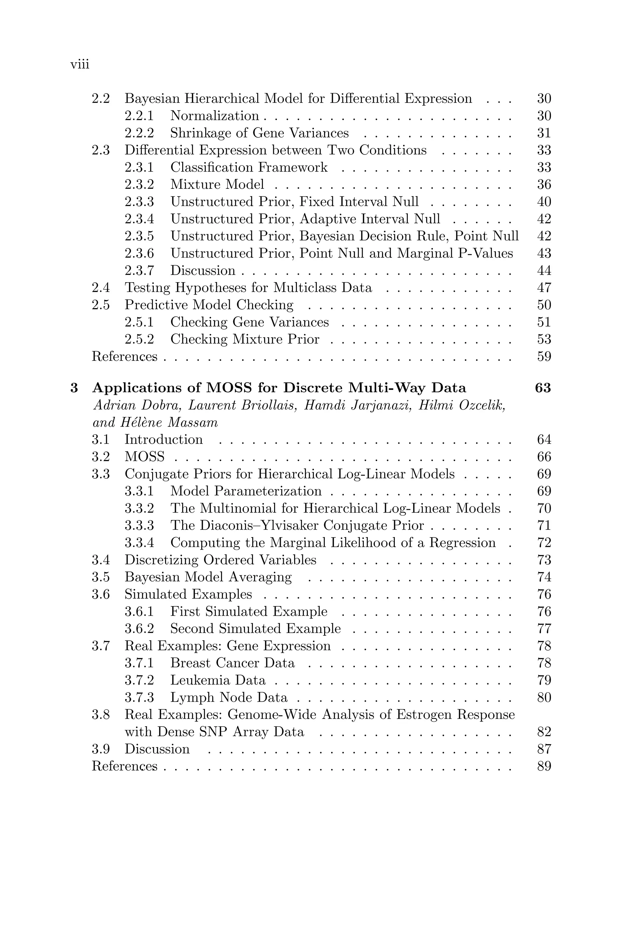
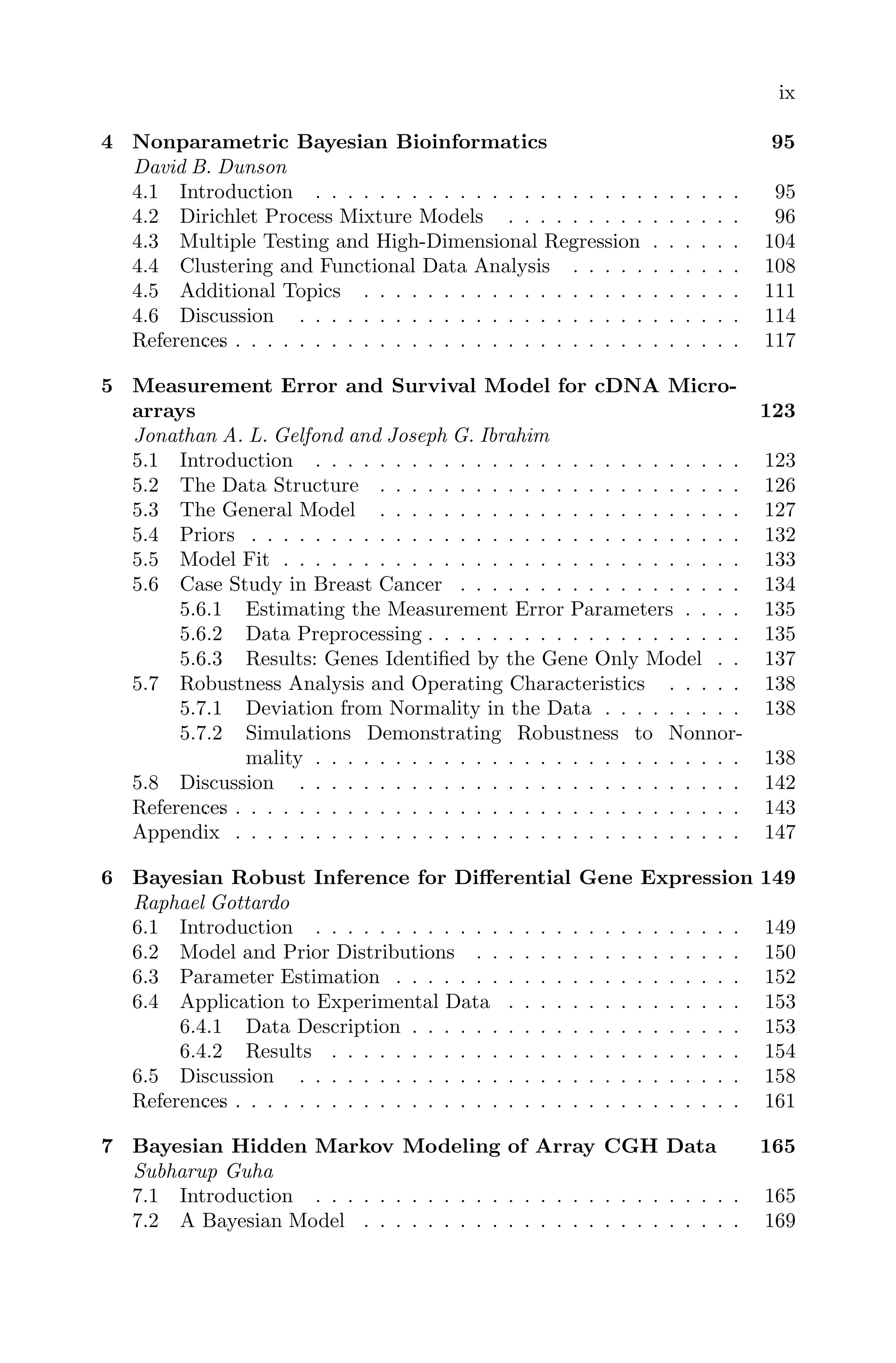


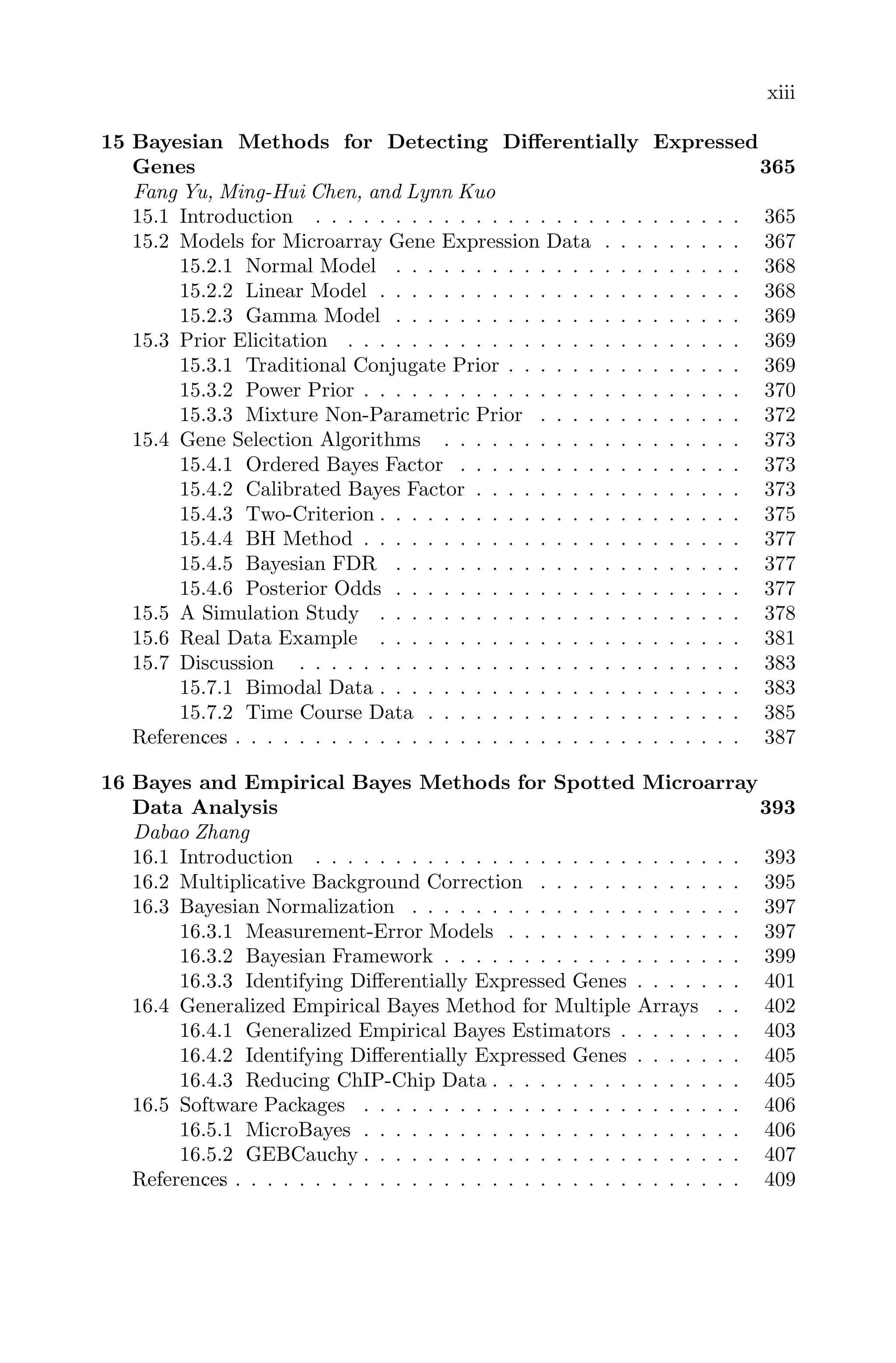

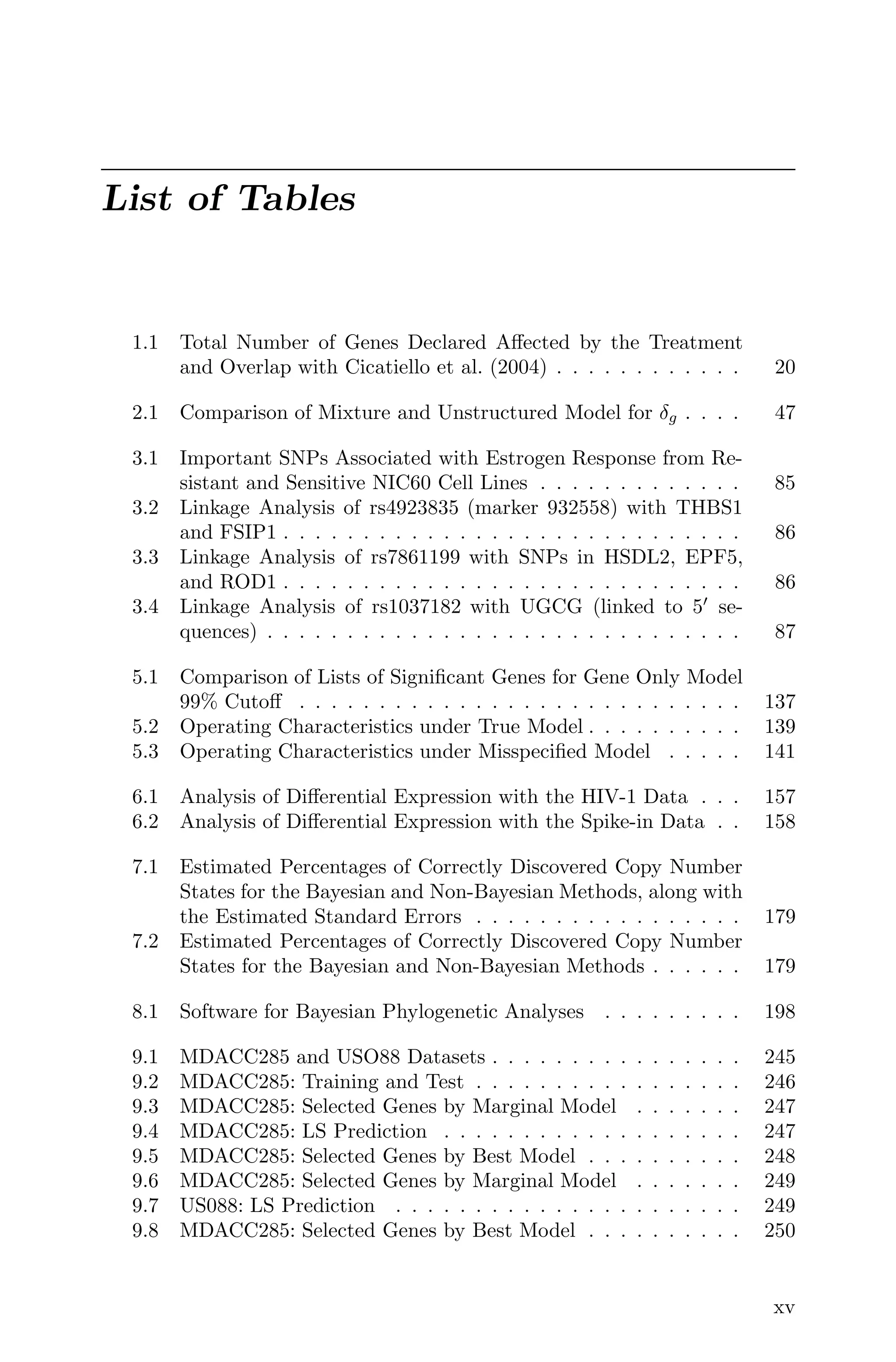
![xix
5.4 Scaled residuals with normal density curve. . . . . . . . . . . 139
5.5 Estimation of regression parameter with 95% HPD under mis-
specified error model. . . . . . . . . . . . . . . . . . . . . . . . 140
5.6 Estimation of latent expression under misspecified error model. 141
6.1 BRIDGE posterior probabilities . . . . . . . . . . . . . . . . . 156
7.1 Breast cancer specimen S0034 from Snijders et al. (2001) . . 167
7.2 Array CGH profiles of some pancreatic cancer specimens . . . 174
7.3 Array CGH profile of chromosome 13 of specimen GBM31 . . 176
7.4 Partial profile of chromosome 7 of specimen GBM29 . . . . . 177
7.5 Bayesian versus non-Bayesian approaches . . . . . . . . . . . 181
7.6 Simulated data set . . . . . . . . . . . . . . . . . . . . . . . . 182
7.7 Estimated means Ê[μj|Y ] for three independently generated
data sets (shown by solid, dashed, and dotted lines) plotted
against . . . . . . . . . . . . . . . . . . . . . . . . . . . . . . 183
8.1 Deep coalescence, with the contained gene tree (dashed line)
failing to coalesce in the ancestral population of species B and
C, leading to the allele sampled in B being more closely related
to allele in A, rather than the true sister species, C. . . . . . 205
8.2 Majority-rule consensus tree phylogeny of 178 species of true
frogs of the subfamily Raninae. Branches with posterior proba-
bility 0.9 are denoted by black dots at the descendant node.
Empty circles denote nodes on branches with posterior proba-
bility between 0.7 and 0.9. Stars indicate three species of frogs
endemic to the Indonesian island of Sulawesi. An arrow indi-
cates the only clade that was in the no-clock consensus tree but
not in the relaxed-clock consensus tree. . . . . . . . . . . . . . 216
8.3 Comparison of posterior probabilities of clades under the no-
clock and relaxed clock approaches, as estimated under 4 in-
dependent runs of 200 million generations each under each ap-
proach. . . . . . . . . . . . . . . . . . . . . . . . . . . . . . . . 217
10.1 ROC curves of the Bayesian methods. . . . . . . . . . . . . . 265
11.1 An example of Bayesian networks. . . . . . . . . . . . . . . . 272
11.2 Sample paths produced by SAMC and MH for the simulated
example. . . . . . . . . . . . . . . . . . . . . . . . . . . . . . . 282
11.3 The maximum a posteriori network structures learned by
SAMC and MH for the simulated example. . . . . . . . . . . 282
11.4 Progression paths of minimum energy values produced by
SAMC and MH for the simulated example. . . . . . . . . . . 284
11.5 Progression paths of minimum energy values produced by
SAMC and MH for the yeast cell cycle example. . . . . . . . 285](https://image.slidesharecdn.com/1021195-250521170514-458f548e/75/Bayesian-Modeling-In-Bioinformatics-Dey-D-Ghosh-S-Mallick-B-Eds-24-2048.jpg)

![xxi
13.1 Estimated survival function for breast carcinomas data using
RVM model. . . . . . . . . . . . . . . . . . . . . . . . . . . . 332
13.2 Estimated survival function for breast carcinomas data using
SVM model. . . . . . . . . . . . . . . . . . . . . . . . . . . . . 333
13.3 Estimated survival function for DLBCL data using RVM
model. . . . . . . . . . . . . . . . . . . . . . . . . . . . . . . . 334
13.4 Estimated survival function for DLBCL data using SVM
model. . . . . . . . . . . . . . . . . . . . . . . . . . . . . . . . 335
14.1 Raw data. The left panel shows the recorded spectra for normal
samples. The right panel shows the spectra for tumor samples.
The X axis are the m/z values. . . . . . . . . . . . . . . . . . 346
14.2 p(J | Y ) and p(Jk | Y ). The histogram in the left panel shows
the posterior probabilities for the number of distinct peaks. We
find the posterior mode around 18 peaks. The boxplots (right
panel) summarize the posterior distributions p(Jk | Y ). The
number of terms in the baseline mixtures was constrained at
Jk ≤ 5. . . . . . . . . . . . . . . . . . . . . . . . . . . . . . . 355
14.3 E[fk(m) | Y, xk = x]. Estimated spectrum for normal and tu-
mor samples. . . . . . . . . . . . . . . . . . . . . . . . . . . . 356
14.4 Posterior inference defines a probability model on the unknown
spectra. The two panels show ten draws from p(fk | Y ) for
xk = 0 (left) and xk = 1 (right). . . . . . . . . . . . . . . . . . 356
14.5 E(1 − λj | Y ). Posterior expected probability of differential
expression for the reported peaks. . . . . . . . . . . . . . . . . 357
14.6 Detected proteins. The figure plots the posterior estimated
weights E(wxj | Y ) against mass/charge ratios E(j | Y ). Panel
(a) plots the average weight E(wxj | Y ), averaging over all it-
erations that reported a protein peak at j. Panel (b) scales
the average weight by the probability of a peak being detected
at j (i.e., no detection is counted as w = 0). For genes with
E(λj | Y ) 0.5 we plot the posterior expectation of w0j. For
differentially expressed genes we plot posterior expectations for
wxj for both conditions, x = 0, 1, linked with a line segment.
Only proteins with posterior expected weight greater or equal
to 0.05 are shown. . . . . . . . . . . . . . . . . . . . . . . . . 357
14.7 Proteins included in a panel of biomarkers to classify samples
according to biologic condition x. Let ER = {1, . . . , R} denote
the locations of peaks, i.e., proteins, included in a subset of size
R. The figure plots for each location r the minimum size R of
subsets that include r. . . . . . . . . . . . . . . . . . . . . . 358
14.8 Some aspects of the MCMC simulation. The left panel plots
the imputed number of proteins J against iteration. The right
panel plots the locations j of the imputed beta kernels (x-axis)
over iterations (y-axis). . . . . . . . . . . . . . . . . . . . . . 358](https://image.slidesharecdn.com/1021195-250521170514-458f548e/75/Bayesian-Modeling-In-Bioinformatics-Dey-D-Ghosh-S-Mallick-B-Eds-26-2048.jpg)


![2 Bayesian Modeling in Bioinformatics
1.2 Introduction
Gene expression levels in a given cell can be influenced by different fac-
tors, namely pharmacological or medical treatments. The response to a given
stimulus is usually different for different genes and may depend on time. One
of the goals of modern molecular biology is the high-throughput identifica-
tion of genes associated with a particular treatment or biological process of
interest. The recently developed technology of microarrays allows one to si-
multaneously monitor the expression levels of thousands of genes. Although
microarray experiments can be designed to study different factors of interest,
in this paper, for simplicity, we consider experiments involving comparisons
between two biological conditions (for example, “control” and “treatment”)
made over the course of time.
The data may consist of measurements of the expression levels of N genes
in two distinct independently collected samples made over time [0,T] (the,
so called,“two-sample problem”), or measurements of differences in the ex-
pression levels between the two samples (the “one-sample problem”). In both
cases, the objective is first to identify the genes that are differentially ex-
pressed between the two biological samples and then to estimate the type of
response. Subsequently, the curves may undergo some kind of clustering in
order to group genes on the basis of their type of response to the treatment.
The problem represents a significant challenge since the number of genes
N is very large, while the number of time points n where the measurements
are made is rather small and, hence, no asymptotic method can be used. The
data is contaminated by usually non-Gaussian heavy-tailed noise. In addi-
tion, non-uniform sampling intervals and missing or multiple data makes time
series microarray experiments unsuitable to classical time-series and signal
processing algorithms.
In the last decades the statistical literature has mostly addressed static mi-
croarray experiments, see Efron et al. (2001), Lonnstedt and Speed (2002),
Dudoit et al. (2002), Kerr et al. (2000), Ishwaran and Rao (2003), among
many others. The analysis of time-course microarray was mainly carried out by
adapting some existing methodologies. For example, SAM version 3.0 software
package—originally proposed by Tusher et al. (2001) and later described in
Storey et al. (2003a, 2003b)—was adapted to handle time-course data by con-
sidering the time points as different groups. In a similar manner, the ANOVA
approach by Kerr et al. (2000) and Wu et al. (2003) was applied to time-course
experiments by treating the time variable as a particular experimental factor.
Similar approaches have been considered by Di Camillo et al. (2005) and the
Limma package by Smyth (2005), while the paper of Park et al. (2003) uses
linear model regression combined with ANOVA analysis. All these methods
can be useful when very short time-course experiments have to be analyzed
(3-4 time points), however they have the shortcoming of applying statistical](https://image.slidesharecdn.com/1021195-250521170514-458f548e/75/Bayesian-Modeling-In-Bioinformatics-Dey-D-Ghosh-S-Mallick-B-Eds-33-2048.jpg)


![Estimation and Testing in Time-Course Microarray Experiments 5
different time points in [0, T ] where the sampling grid t(1)
, t(2)
, . . . , t(n)
is not
necessarily uniformly spaced. For each array, the measurements consist of N
normalized log2-ratios zj,k
i , where i = 1, . . . , N, is the gene number, index j
corresponds to the time point t(j)
and k = 1, . . . , k
(j)
i , k
(j)
i ≥ 0, accommodates
for possible technical or biological replicates at time t(j)
. Note that usually,
by the structure of the experimental design, k
(j)
i are independent of i, i.e.,
k
(j)
i ≡ k(j)
with M =
n
j=1 k(j)
being the total number of records. However,
since some observations may be missing due to technical errors in the experi-
ment, we let k
(j)
i to depend on i so that the total number of records for gene
i is
Mi =
n
j=1
k
(j)
i . (1.1)
The number of time points is relatively small (n ≈ 10) and very few replica-
tions are available at each time point (k
(j)
i = 0, 1, . . . K where K = 1, 2, or
3) while the number of genes is very large (N ≈ 10, 000).
1.3.2 Data Structure in the Multi-Sample Case
Consider data consisting of measurements of the expression levels of N
genes in two or more distinct independently collected samples made over time
[0,T].
We note that, when the number of samples is two, the objective is first to
identify the genes that are differentially expressed between the two samples
and then to estimate the type of response. On the other hand, when more
samples are considered one may be interested in detecting both genes that are
differentially expressed under at least one biological condition or some specific
contrasts, in a spirit that is similar to the multi-way ANOVA model and then
to estimate the type of effect. In general, the problem can be formulated
as follows. For sample ℵ, ℵ = 1, · · · , H, data consists of the records zj,k
ℵi , i =
1, · · · , N, on N genes, which are taken at time points t
(j)
ℵ ∈ [0, T ], j = 1, .., nℵ.
For gene i at a time point t
(j)
ℵ , there are k
(j)
ℵi (with k
(j)
ℵi = 0, 1, . . ., K) records
available, making the total number of records for gene i in sample ℵ to be
Mℵi =
n
j=1
k
(j)
ℵi . (1.2)
Note that in this general setup it is required neither that the observations
for the H samples are made at the same time points nor that the number
of observations for different samples is the same. This model can be applied
when observations on the H samples are made completely separately: the only
requirement is that the samples are observed over the same period of time.
The orders of magnitude of N, n, and K are the same as in the one-sample
case.](https://image.slidesharecdn.com/1021195-250521170514-458f548e/75/Bayesian-Modeling-In-Bioinformatics-Dey-D-Ghosh-S-Mallick-B-Eds-36-2048.jpg)
![6 Bayesian Modeling in Bioinformatics
1.4 Statistical Methods for the One-Sample Microarray
Experiments
In this section we present the more recent and important methods for the
one-sample microarray time-course experiments.
1.4.1 Multivariate Bayes Methodology
Tai and Speed (2006) suggest multivariate Bayes methodology for identifi-
cation of differentially expressed genes. Their approach is specifically designed
for longitudinal experiments where each replicate refers to one individual. The
technique requires that for each gene the number of replicates k
(j)
i is constant
for all time points k
(j)
i = ki, so that for each gene i there are ki independent
n-dimensional observations zi,k = (z1,k
i , . . . , zn,k
i )T
∈ Rn
, k = 1, . . . , ki. Each
vector is modeled using multivariate normal distribution zi,k ∼ Nn(Iiμi, Σi)
where Ii is the Bernoulli random variable, which is equal to 1 when gene i
is differentially expressed and zero otherwise. For each gene i, the following
hierarchical Bayesian model is built:
μi|Σi, Ii = 1 ∼ N(0, η−1
i Σi)
μi|Σi, Ii = 0 = 0
Σi ∼ InverseWishart(νi, νiΛ−1
i )
P(Ii = 0) = π0.
Here νi, ηi and Λi are gene-specific parameters to be estimated from the
data, while π0 is a global user-defined parameter. To test whether a gene is
differentially expressed, Tai and Speed (2006) evaluate posterior odds of Ii = 1
Oi =
P(Ii = 1|zi,1, · · · , zi,ki )
P(Ii = 0|zi,1, · · · , zi,ki )
. (1.3)
Denote by z̄i and Si the mean and the sample covariance matrix of the vectors
zi,1, · · · , zi,ki , and let
S̃i = [(ki − 1)Si + νiΛi]/(ki − 1 + νi) and t̃i =
kiS̃
−1/2
i ¯
zi
be the moderated sample covariance matrix and multivariate t-statistic. Then,
posterior odds (1.3) can be rewritten as
1 − π0
π0
ηi
ηi + ki
n/2
ki − 1 + νi + t̃T
i t̃i
ki − 1 + νi + (ki + ηi)−1ηt̃T
i t̃i
(ki+νi)/2
. (1.4)
Unknown gene specific parameters νi, ηi and Λi are estimated using a ver-
sion of empirical Bayes approach described in Smyth (2004) and are plugged](https://image.slidesharecdn.com/1021195-250521170514-458f548e/75/Bayesian-Modeling-In-Bioinformatics-Dey-D-Ghosh-S-Mallick-B-Eds-37-2048.jpg)


![Estimation and Testing in Time-Course Microarray Experiments 9
where zi = (z1,1
i . . . z
1,k
(1)
i
i , · · · , zn,1
i , . . . z
n,k
(n)
i
i )T
∈ RMi
is the column vec-
tor of all measurements for gene i (see (1.1)), ci = (c0
i , . . . , cLi
i )T
∈
RLi+1
is the column vector of the coefficients of si(t) in the chosen basis,
ζi = (ζ1,1
i , . . . , ζ
1,k
(1)
i
i , · · · , ζn,1
i , . . . , ζ
n,k
(n)
i
i )T
∈ RMi
is the column vector of
random errors and Di is the Mi × (Li + 1) block design matrix the j-row of
which is the block vector [φ0(t(j)
) φ1(t(j)
) . . . φLi (t(j)
)] replicated k
(j)
i times.
The following Bayesian model is imposed on the data:
zi | Li, ci, σ2
∼ N(Dici, σ2
IMi );
Li ∼ Pois∗
(λ, Lmax), Poisson with parameter λ truncated at Lmax ;
ci | Li, σ2
∼ π0δ(0, . . . , 0) + (1 − π0)N(0, σ2
τ2
i Q−1
i ).
Here, π0 is the prior probability that gene i is not differentially expressed.
Matrix Qi is a diagonal matrix that accounts for the decay of the coefficients
in the chosen basis and depends on i only through its dimension.
Parameter σ2
is also assumed to be a random variable σ2
∼ ρ(σ2
), which
allows to accommodate possibly non-Gaussian errors (quite common in mi-
croarray experiments), without sacrificing closed form expressions for estima-
tors and test statistics. In particular, the following three types of priors ρ(·)
are considered:
case 1: ρ(σ2
) = δ(σ2
− σ2
0), the point mass at σ2
0. The marginal distribution
of the error is normal.
case 2: ρ(σ2
) = IG(γ, b), the Inverse Gamma distribution. The marginal
distribution of the error is Student T .
case 3: ρ(σ2
) = cμσ(M−1)
e−σ2
μ/2
, where M is the total number of arrays
available in the experimental design setup. If the gene has no missing
data (Mi = M), i.e. all replications at each time point are available,
then the marginal distribution of the error is double exponential.
The procedure proposed in Angelini et al. (2007) is carried out as follows.
The global parameters ν, λ and
Lmax are defined by a user. The global pa-
rameters π0 and case-specific parameters, σ2
0 for case 1, γ and b for case 2,
and μ for case 3 are estimated from the data using records on all the genes
that have no missing values. The gene-specific parameter τ2
i is estimated by
maximizing the marginal likelihood p(zi) while Li is estimated using the mode
or the mean of the posterior pdf p(Li|zi).
In order to test the hypotheses H0i : ci ≡ 0 versus H1i : ci ≡ 0 for
i = 1, . . . , N, and estimate the gene expression profiles, Angelini et al. (2007)
introduce, respectively, the conditional and the averaged Bayes factors
BFi(L̂i) =
(1 − π0)P(H0i|zi, L̂i)
π0P(H10i|zi, L̂i)
, BFi =
(1 − π0)P(H0i|zi)
π0P(H10i|zi)
.](https://image.slidesharecdn.com/1021195-250521170514-458f548e/75/Bayesian-Modeling-In-Bioinformatics-Dey-D-Ghosh-S-Mallick-B-Eds-40-2048.jpg)
![10 Bayesian Modeling in Bioinformatics
Bayes factors can be evaluated explicitly using the following expressions
BFi(L̂i) = A0i(L̂i)/A1i(L̂i), BFi =
Lmax
Li=0
gλ(Li)A0i(Li)
(1.7)
×
Lmax
Li=0
gλ(Li)A1i(Li)
(1.8)
where
A0i(Li) = F(Mi, zT
i zi), A1i(Li)
= τ
−(Li+1)
i [(Li + 1)!]ν
|Vi|−1/2
F(Mi, Hi(zi)),
Vi = DT
i Di + τ−2
i Qi, Hi(zi) = zT
i zi − zT
i DiV−1
i DT
i zi,
and
F (A, B) =
⎧
⎪
⎪
⎪
⎨
⎪
⎪
⎪
⎩
σ−2A
0 e−B/2σ2
0 in case 1,
Γ(A+γ)
Γ(γ) b−A
(1 + B
2b )−(A+γ)
in case 2,
B(M+1−2A)/4
μ(M+1+2A)/4
2(M−1)/2 Γ((M+1)/2)
K((M+1−2A)/2)(
√
Bμ) in case 3,
Here Kh(·) is the Bessel function of degree h (see Gradshteyn and
Ryzhik [1980] for the definition and Angelini et al. [2007]) for additional de-
tails).
The authors note that the two Bayes factors defined in (1.7) lead to an al-
most identical list of selected genes with the selection on the basis of BFi being
more theoretically sound but also slightly more computationally expensive.
Bayes factors BFi, although useful for independent testing of the null hy-
potheses H0i, i = 1, . . . , N, do not account for the multiplicity when test-
ing a large number of hypotheses simultaneously. In order to take into ac-
count multiplicity, the authors apply a Bayesian multiple testing procedure of
Abramovich and Angelini (2006).
Finally, the coefficients ci for the differentially expressed genes are estimated
by the posterior means
ĉi =
(1 − π0)/π0
BFi(L̂i) + (1 − π0)/π0
DT
i Di + τ̂−2
i Qi
−1
DT
i zi.
Methodology of Angelini et al. (2007) is much more computationally effi-
cient than that of Storey et al. (2005): all Bayesian calculations use explicit
formulae and, hence, are easy to implement. In addition, by allowing a different
number of basis functions for each curve, it avoids the need to pre-determine
the group of the most significant genes in order to select the dimension of](https://image.slidesharecdn.com/1021195-250521170514-458f548e/75/Bayesian-Modeling-In-Bioinformatics-Dey-D-Ghosh-S-Mallick-B-Eds-41-2048.jpg)

![12 Bayesian Modeling in Bioinformatics
in time of its expression level is governed by a function sℵi(t) and each of
the measurements zj,k
ℵi involves some measurement error. For what concerns
the two-sample problem, the quantity of interest is the difference between
expression levels si(t) = s1i(t) − s2i(t). In particular, si(t) ≡ 0 means that
gene i is not differentially expressed between the two samples, while si(t) ≡ 0
indicates that it is. In the case of a multi-sample setup, a variety of statistical
hypotheses can be tested. However, in the present paper we focus on the
problem of identification of the genes that are differentially expressed under
at least one biological condition.
Although mathematically the two-sample setup appears homogeneous, in
reality it is not. In fact, it may involve comparison between the cells under
different biological conditions (e.g., for the same species residing in different
parts of the habitat) or estimating an effect of a treatment (e.g., effect of
estrogen treatment on a breast cell). The difference between the two cases
is that, in the first situation, the two curves s1i(t) and s2i(t) are truly in-
terchangeable, while in the second case they are not: s2i(t) = s1i(t) + si(t),
where si(t) is the effect of the treatment. In order to conveniently distinguish
between those cases, Angelini et al. (2009) refer to them as “interchangeable”
and “non-interchangeable” models. It is worth noting that which of the two
models is more appropriate should be decided rather by a biologist than a
statistician.
Similarly to the one-sample case, Angelini et al. (2009) expand each function
sℵi(t) over a standard orthogonal basis on the interval [0, T ] (see eq. (1.5)),
characterizing each sℵi(t) by the vector of its coefficients cℵi. The number of
coefficients Li +1 can vary from gene to gene but it is required to be the same
in all samples. Similarly to the one-sample case (see eq. (1.6)) one has
zℵi = Dℵicℵi + ζℵi (1.9)
where zℵi = (z1,1
ℵi . . . z
1,k
(1)
ℵi
ℵi , · · · , zn,1
ℵi , . . . z
n,k
(n)
ℵi
ℵi )T
∈ RMℵi
is the column vector
of all measurements for gene i in sample ℵ, cℵi is the column vector of the
coefficients of sℵi(t), ζℵi is the column vector of random errors and Dℵi is
the Mℵi × (Li + 1) block design matrix the j-row of which is the block vector
[φ0(t
(j)
ℵ ) φ1(t
(j)
ℵ ) . . . φLi (t
(j)
ℵ )] replicated k
(j)
ℵi times. The following Bayesian
model is imposed
zℵi | Li, cℵi, σ2
∼ N(Dℵicℵi, σ2
IMℵi
)
Li ∼ Pois∗
(λ, Lmax), Poisson with parameter λ truncated at Lmax .
The vectors of coefficients cℵi are modeled differently in the interchangeable
and noninterchangeable cases.
Interchangeable setup
Since the choice of which sample is the first, which is the second and so
on, is completely arbitrary, it is reasonable to assume that a-priori vec-
tors of the coefficients are either equal to each other or are independent](https://image.slidesharecdn.com/1021195-250521170514-458f548e/75/Bayesian-Modeling-In-Bioinformatics-Dey-D-Ghosh-S-Mallick-B-Eds-43-2048.jpg)
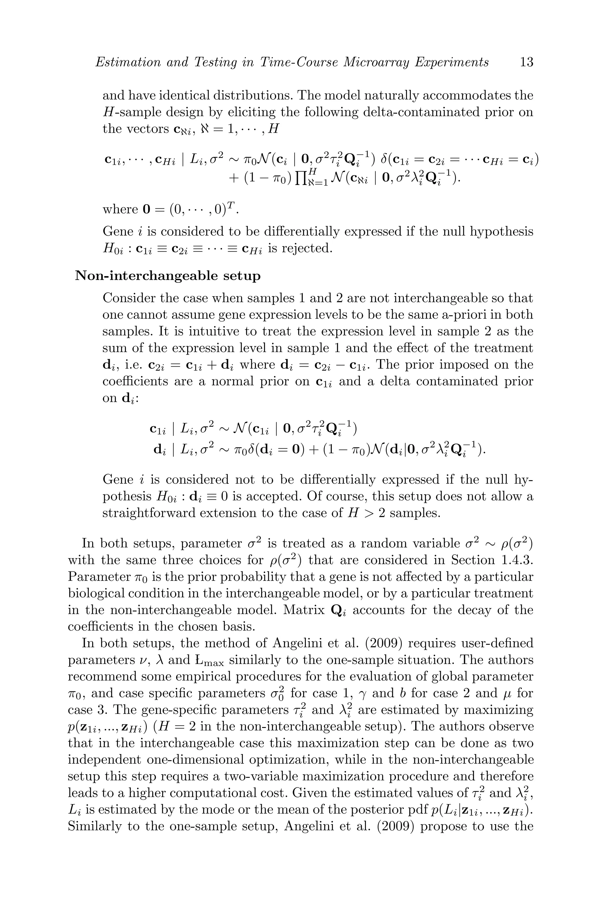
![14 Bayesian Modeling in Bioinformatics
Bayes factors BFi for testing hypotheses H0i and again the two kinds of Bayes
factor are considered
BFi(L̂i) =
(1 − π0)P(H0i|z1i, ..., zHi, L̂i)
π0P(H10i|z1i, ..., zHi, L̂i)
,
BFi =
(1 − π0)P(H0i|z1i, ..., zHi)
π0P(H10i|z1i, ..., zHi)
, (1.10)
with H = 2 in the non-interchangeable setup. The multiplicity control is car-
ried out similarly to the one-sample situation by using the Bayesian procedure
of Abramovich and Angelini (2006).
For brevity, we do not report the formulae since they are quite complex
mathematically and require some elaborate matrix manipulations, especially
in the non-interchangeable setup (they can be found in Angelini et al. [2009]).
Similarly to the one sample case, Angelini et al. (2009) also provide analytic
expressions for the estimators of the gene expression profiles in both inter-
changeable and non-interchangeable setups.
Empirical Bayes functional data approach was also considered in the papers
of Tai and Speed (2007) and Hong and Li (2006).
Tai and Speed (2008) extend their multivariate Bayes methodology to the
multi-sample cross-sectional design where the biological conditions under in-
vestigation are interchangeable. The authors consider a Bayesian functional
data approach. They expand the mean of the multivariate normal distribution,
which models the data over a splines basis, and assume the number of basis
functions to be a fixed constant chosen in advance. The model is similar to
that of Angelini et al. (2009) with ρ(σ2
) being Inverse Gamma (case 2 above).
Also, the procedure only ranks the genes without providing any automatic
cutoff point to select the differentially expressed genes.
Hong and Li (2006) propose a Bayesian functional data model for detect-
ing differentially expressed genes in the case of cross-sectional design and
non-interchangeable biological conditions. The model is somewhat similar
to the non-interchangeable setup of Angelini et al. (2009) described above.
Hong and Li (2006) expand the gene expression profiles over a polynomial
or B-spline basis of fixed degree, which is globally estimated by cross val-
idation. The authors impose a prior on di similar to (1.5.2) and treat c1i
as unknown nuisance parameters. They also elicit an Inverse Gamma prior
on the error variance allowing experiment-specific, gene-specific, and time-
specific errors (σ2
)
(j)
ℵ,i. The gene-specific parameters and the hyperparameters
of the model are estimated using computationally expensive Monte Carlo EM
algorithm.
In order to test hypotheses H0i, Hong and Li (2006) evaluate posterior
probabilities that di ≡ 0 and then rank the genes accordingly. Alternatively,
they provide an automatic cutoff point by controlling the false discovery rate
(FDR) with a procedure similar to Storey (2003c). Similarly to Angelini et
al. (2009), Hong and Li (2006) method does not require the measurements for](https://image.slidesharecdn.com/1021195-250521170514-458f548e/75/Bayesian-Modeling-In-Bioinformatics-Dey-D-Ghosh-S-Mallick-B-Eds-45-2048.jpg)
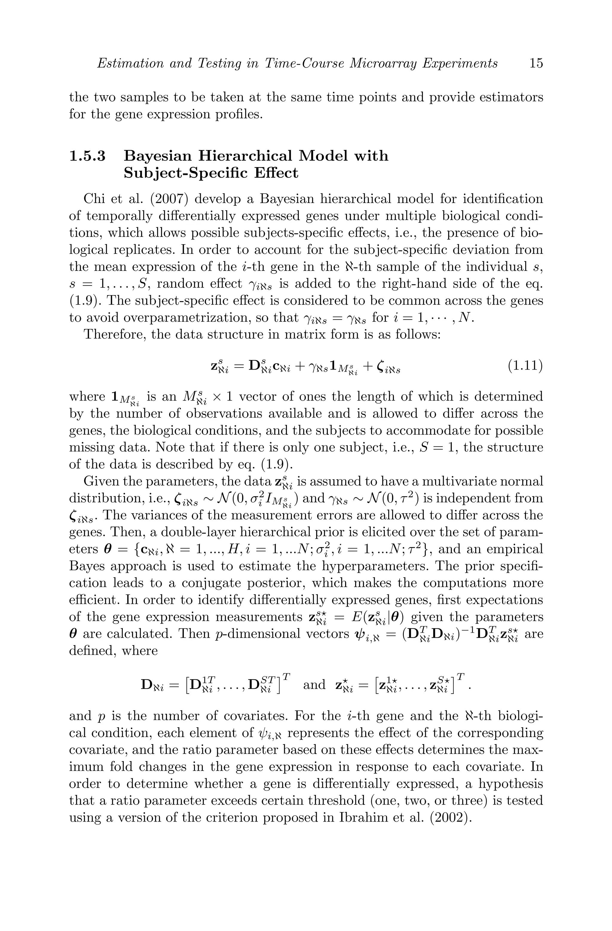
![16 Bayesian Modeling in Bioinformatics
1.5.4 Hidden Markov Models
Yuan and Kendziorski (2006) introduce hidden Markov chain based
Bayesian models (HMM) for analysis of the time series microarray data. It
is assumed that the vector of expression levels for gene i at time t under
the biological conditions ℵ = 1, · · · , H, is governed by an underlying state of
a hidden Markov chain, i.e., (z
(t)
i |s
(t)
i = l) ∼ flt(z
(t)
i ) where l is the possi-
ble state of the HMM, and the length of the vector is equal to the number
of measurements at time t under all H biological conditions. In the case of
H = 2 biological conditions, the HMM has two states: genes are either equally
expressed (l = 1) or differentially expressed (l = 2). In a general situation, the
number of states of the HMM is equal to the number of nonempty subsets of
the set with H elements.
The vectors z
(t)
i are assumed to have means μ
(t)
i , which are distributed
according to some prior pdf. Unknown hyperparameters of the model are es-
timated by maximizing the marginal likelihood of the data on the basis of a
version of EM algorithm. In the case of H = 2, the decision on whether gene i
is differentially expressed is made by evaluating posterior odds of P(s
(t)
i = 2);
for general case, posterior probabilities can be evaluated for each configu-
ration. In the particular version of the HMM model described in Yuan and
Kendziorski (2006), the authors use Gamma distribution for both the data
and the underlying means.
The paper provides a paradigm for modeling time series microarray data,
which is very different from the methodologies described above. However,
the weakness of the approach is that it tests whether a gene is differentially
expressed at a particular time point not overall, thus, ignoring the temporal
dependence between the expressions.
1.6 Software
Microarray data analysis is a very active area of research and several soft-
ware packages have been recently released. Private companies who produce
microarray equipment have their proprietary software, and several commer-
cial software packages are now available. The use of the commercial software
systems is however often limited by the cost of the license and the delay
in incorporating innovative research techniques into the new releases. On
the other hand, there are also a number of open source software packages
for analysis of microarray data, the most widely used ones being distributed
by Bioconductor (http://www.bioconductor.org/), an open source software
project for the analysis and comprehension of genomic data (see Gentleman
et al. [2004] and Gentleman et al. [2005]), which is based on R (http://www.
r-project.org/).](https://image.slidesharecdn.com/1021195-250521170514-458f548e/75/Bayesian-Modeling-In-Bioinformatics-Dey-D-Ghosh-S-Mallick-B-Eds-47-2048.jpg)
![Estimation and Testing in Time-Course Microarray Experiments 17
Several packages include tools for analysis of time course microarray ex-
periments; however, majority of them use methodology constructed for static
microarray experiments and for a specific experimental design (see, for exam-
ple, SAM version 3.0 software package originally proposed by Tusher et al.
[2001] and later described in Storey et al. [2003a, 2003b], MAANOVA by Kerr
et al. [2000] and Wu et al. [2003] and the Limma package by Smyth [2005]). On
the other hand, recently other software packages have been developed that are
specifically designed for analysis of time course microarray data. It should be
noted that when the time series are very short (n = 3 or 4), the functional data
analysis methodsm which are discussed in this review, are not recommended
since simpler methods are more advantageous in this case, e.g., MaSigPro, the
linear regression approach of Conesa et al. (2006), the STEM package by Ernst
and Bar-Joseph (2006), or the Timecourse package of Tai and Speed (2006).
In what follows, we briefly present the software packages that implement
some of the methodologies discussed in this review. We note that all these
software packages require data to be already pre-processed to remove system-
atic sources of variation (see Gentleman et al. [2005] or Parmigiani et al. [2003]
for discussion of the software).
EDGE
Software package EDGE (see Leek et al. [2006] for details) implements
the functional data approach proposed in Storey et al. (2005). The software
is distributed as a stand-alone package and can be freely downloaded from
http://www.genomine.org/edge/ for academic non-commercial users. It re-
lies on R language and Bioconductor in the background, however a user does
not need to know R to use it but only to interact with a graphical user friendly
interface.
Applications of EDGE are not limited to time-course microarray data:
EDGE can also be employed for static experiments. Moreover, it also has
some useful utilities that allow one to explore input data, such as drawing
boxplots, checking for the presence of missing data, and imputing them with
the “K nearest neighbor” (KNN) algorithm. In fact, EDGE does not allow
missing data in the course of statistical analysis.
The software requires a user to define a number of permutations to be
performed for evaluating the p-values. The shortcoming of this feature is
that a relatively small number of permutations lead to a granularity prob-
lem (the p-values are quantized), while increasing number of permutations
usually improves approximation of the p-values, but leads to a very high com-
putational cost.
TIMECOURSE
The package Timecourse implements the multivariate Bayesian approach
of Tai and Speed (2006) for both the one-sample and the two-sample
designs. Timecourse is distributed as contributed package within Bioconductor](https://image.slidesharecdn.com/1021195-250521170514-458f548e/75/Bayesian-Modeling-In-Bioinformatics-Dey-D-Ghosh-S-Mallick-B-Eds-48-2048.jpg)
![18 Bayesian Modeling in Bioinformatics
(http://bioconductor.org/packages/2.1/bioc/html/timecourse.html),
thus, its application requires the knowledge of the R-language. Although this
can be advantageous to R users since Timecourse allows them to interact with
other tools that are developed under Bioconductor project, this feature can
be rather intimidating for a biologist or a person unfamiliar with R language.
For example, the package neither allows missing data or unequal number of
replicates, nor it provides any tools for handling these problems, although
expert R users can import such tools from other R packages.
Since all calculations are based on explicit formulae, the computational cost
of Timecourse is very low. However, the package only ranks the genes in the
order of statistical significance without providing an automatic cutoff point
to identify which genes are differentially expressed. Finally, the results of the
analysis are completely independent of the actual time measurements, so that
it is preferable to apply the software only when the grid is equispaced. On
the other hand, the package can be successfully applied for short time-course
experiments.
Current version of Timecourse does not include the functional approach
described in Tai and Speed (2007), which we hope will be added in future
releases.
BATS
The software package BATS (see Angelini et al. [2008]) implements the
Bayesian functional approach proposed by Angelini et al. (2007). It is also
distributed as a stand-alone software that can be freely downloaded from
http://www.na.iac.cnr.it/bats/.
The software has a friendly graphical user interface. Although it is written
in MATLAB R
, it does not require a user to know MATLAB R
.
Similarly to EDGE, BATS also has some helpful utilities, which allow to plot
and filter the data, and compare the lists of differentially expressed genes ob-
tained under different options. Due to flexibility of the methodology, the issue
of missing data does not arise. Furthermore, by using the Bayesian methodol-
ogy in combination with the functional data approach, BATS can successfully
handle various other technical difficulties such as non-uniform sampling inter-
vals, presence of multiple data as well as temporal dependence between obser-
vations for each gene, which are not fully addressed by EDGE and Timecourse.
Since all calculations are based on explicit expressions, the computational cost
of BATS is very low and is comparable to that of Timecourse.
The current version of BATS can be applied to a one-sample case only. The
software allows different number of basis functions for each curve si(t), thus
improving the fit and avoiding the need to pre-determine the most significant
genes to select the dimension of the approximation.
The two-sample and the multi-sample experimental designs will be accom-
modated in future releases by following methodology of Angelini et al. (2009)
described above.](https://image.slidesharecdn.com/1021195-250521170514-458f548e/75/Bayesian-Modeling-In-Bioinformatics-Dey-D-Ghosh-S-Mallick-B-Eds-49-2048.jpg)
![Estimation and Testing in Time-Course Microarray Experiments 19
1.7 Comparisons between Techniques
Each of the methods presented above have been tested on simulated and
real data (see Storey et al. [2005], Tai and Speed [2006, 2007], Hong and
Li [2006] and Angelini et al. [2007, 2009]). However, each study considered
only a single technique and did not have an objective of comparison be-
tween competitive approaches. To the best of the authors’ knowledge, An-
gelini et al. (2007) and Mutarelli et al. (2008) are the only papers where
a comparative study for the one-sample problem was attempted between the
EDGE software, the R-package Timecourse and BATS software; in the follow-
ing this comparative study is briefly presented (see Angelini et al. [2007] for
details).
Since all three methods apply to different experimental designs, account for
different biological information, and are valid under different assumptions, the
methods were compared using a real data set that does not conform to specific
assumptions. For comparisons, the cDNA microarray dataset of Cicatiello
et al. (2004) was chosen (the data are available on the GEO repository -
http://www.ncbi.nlm.nih.gov/geo/, accession number GSE1864) since it
provides a “biology-guided” selection of significant genes that can be used as
a “benchmark” in comparisons.
The objective of the experiment was to identify genes involved in the es-
trogen response in a human breast cancer cell line and to estimate the type
of the response. Estrogen has a known role in promoting cell proliferation
and thus in cancer development in hormone-responsive tissues such as breast
and ovary. In the original experiment, ZR-75.1 cells were stimulated with a
mitogenic dose of 17β-estradiol, after 5 days of starvation on an hormone-
free medium, and samples were taken after t = 1, 2, 4, 6, 8, 12, 16, 20, 24, 28, 32
hours, with a total of 11 time points covering the completion of a full mitotic
cycle in hormone-stimulated cells. For each time point at least two replicates
were available (three replicates at t = 2, 8, 16).
The data was pre-processed and genes for which more than 20% of values
were missing were removed from further investigation. As a result, the total
number of analyzed genes was 8161 (among them about 350 contained at
least one missing value). Since the EDGE software does not automatically
account for missing values but only suggests a preliminary procedure (K-
nearest-neighbors) for filling them in, the authors repeated the analysis both
using this procedure and filtering out genes with missing values. Timecourse
neither allows missing values nor suggests a specific procedure for treating
them. Moreover, it requires that each time point has the same number of
replicates (different number of replicates are allowed between different genes).
In order to apply Timecourse, all the genes with missing observations were
filtered out, and then the third observations, which was available at time
points t = 2, 8, 16, were discarded.](https://image.slidesharecdn.com/1021195-250521170514-458f548e/75/Bayesian-Modeling-In-Bioinformatics-Dey-D-Ghosh-S-Mallick-B-Eds-50-2048.jpg)