This document describes a model developed by Abbey Chaver and Benjamin LeRoy to optimize Amazon's last-mile transportation costs by determining the optimal number of guaranteed, option, and spot drivers to hire each day. The model sets wages for each driver type such that drivers are indifferent between contract types. It defines terms, makes assumptions, sets up an objective function to minimize total expected costs based on demand distributions, and provides an example solution based on parameter values tested in R code. The model suggests paying for flexibility with option and spot drivers is more cost-efficient than guaranteed drivers.

1. Amazon Logistics
Last Mile Cost Optimization
Abbey Chaver and Benjamin LeRoy
May 4, 2015
Abbey Chaver is a second-year Operations Research and Management Science stu-
dent. She is interested in data science, user experience research, and scalable business
models. She also dabbles in design. To build this model, she drew on knowledge from
Economics, Statistics, and Industrial Engineering courses.
Ben LeRoy is a senior Applied Math and Statistics double major, graduating in De-
cember of this year. He’s interested in data science, statistical modeling, machine-learning,
and all cool statistic stuff. His focuses outside Math and Stats including Economics and
IEOR.
1

2. 1 Challenge
Last-mile transportation is one of Amazon’s biggest marginal costs. Optimizing this
process is challenging due to daily variance in demand. Given a demand distribution
Normal (µ = 12, 000 , σ = 2, 400) on weekdays and Normal (µ = 8, 000, σ = 1, 600) on
weekends, how much should Amazon pay:
1. Guaranteed drivers, who must be paid whether or not there are packages for them
to deliver.
2. Option drivers, who are paid a reservation price to be available but need not be paid
a full wage if there are not packages for them.
3. Spot drivers, who are only paid if they are needed that day.
2 Approach
One of the first questions we considered was whether or not Amazon should pay a premium
wage, or efficiency wage, above the market rate. From looking at labor data, we found that
truckers have a very low rate of voluntary absenteeism - most absenteeism is attributed
to illness or injury. Therefore, offering a higher wage is unlikely to be cost effective. We
recommend paying the market wage.
We made the following assumptions about the contracting process: Each type of driver
is under a contract that once taken, will be filled. We assume that drivers will be willing to
take a contract at the market wage for a guaranteed daily payment. We assume that each
driver takes a uniform packages to deliver for each day. We also assume that option workers
and spot workers, if not hired by Amazon, are able to enter the general spot market, where
they may be able to find work at a wage approximately equivalent to the spot wage that
Amazon offers. While there is reasonably high demand for delivery drivers, we assume that
the probability a driver would find work on the open market is less than 1. Otherwise,
there would be no risk in being a spot driver and all drivers would prefer to be spot drivers.
Essentially, Amazon must set wages for each type of driver such that a driver will be
willing to take any of the three contracts, allowing Amazon to hire the optimal number of
each.
We decided to model the wage as a base rate - the market wage - for each package, plus
an additional premium to compensate drivers for the risk of not being hired by Amazon
for the day. To solve the problem numerically, we set certain parameters at figures we con-
sidered reasonable. However, these figures can and should be adjusted to reflect available
data.
2

3. 3 Model
When building our model, we realized that optimizing total cost required solving for the
number of each type of driver as well as the wage we paid them. We defined these terms
for our calculations:
3.1 Terms
Y: Daily demand for packages to be delivered (distributed Normal(µ, σ) ).
x1: Number of packages allotted to guaranteed drivers
x2: Number of packages allotted to option drivers
x3: Number of packages allotted to spot drivers
c1: Market rate for delivering a single package, paid to guaranteed drivers no matter what.
c2: Risk premium for delivering a single package, paid to option drivers no matter what.
If they are hired that day, they are payed c2 in addition to c1.
c3: Risk premium for delivering a single package, paid to spot drivers only if they are hired
that day, in addition to c1.
s: Reflects the probability that a spot driver will find work on the open market (∈ [0, 1]).
3.2 Relating Terms
We consider the wages c2 and c3 risk premiums, so we need to quantify how much risk is
perceived by a driver in each situation. We also consider c1 to be a market rate that we
cannot set independently, so essentially a constant. We also assume that if an option or
spot driver is not hired by Amazon, they can seek work with other companies. We assume
that the market will perform the same calculation as us, resulting in a spot market wage
of (c1 + c3).
We used a risk-averse utility function to capture a driver’s desire for a guaranteed wage.
By defining c2 and c3 as functions of x1, x2, and x3, we can minimize a total cost function
with respect to fewer variables. We use the relative risk aversion function:
u(c) = (1 − e−γc
)
3

4. 3.3 Option Drivers
First, we want to choose c2 such that a driver is indifferent between c1 and the option
lottery displayed below:
The above diagram leads us to equalize the following equation:
u(c1) = [a · [s · u(c2 + c1 + c3) + (1 − s) · u(c1)] + b · u(c1 + c2)]
Later we will want to express c2 in terms of x1,x2, and c1; the math is worked out in
Math Appendix .
The probability that any certain option driver is hired by Amazon is dependent on
either of these two scenarios occur: Y ≥ (x1 + x2), or x1 ≤ Y ≤ (x1 + x2). A particular
option driver is selected out of all the x2 option drivers (we assume each option driver is
equally likely to be chosen) if x1 ≤ Y ≤ (x1 + x2).
So the probability of getting hired, b, is:
b =
x1+x2
x1
y − x1
x2
P(y)dy + P(Y > x1 + x2)
a = 1 − b
4

5. 3.4 Spot Drivers
Similarly, we want drivers to be indifferent between c1 and the spot lottery:
The above diagram leads us to equalize the following eqation:
u(c1) = [a · [s · u(c1 + c3) + (1 − s) · u(0)] + b · u(c1 + c3)]
You can see how we express c3 as a function of x1,x2 and c1 in Math Appendix.
The optimal value of x3 is essentially infinite: we assume that we will be able to find
enough spot workers to cover all of our demand if we offer a fair wage. However, having
no upper limit to the number of spot drivers available makes it difficult to calculate the
probability that any one spot driver will be hired by Amazon, as we were able to do for
option drivers. Therefore, we assumed that it’s reasonable to solve the problem within three
standard deviations of the distribution: we would almost never expect to hire beyond that.
So we define:
x3 = (µ + 3σ) − (x1 + x2)
Then we can define a spot worker getting hired as the scenario where
Y ≥ (x1 + x2)
and that this driver is selected out of the x3 option drivers. The probability b that this
occurs is:
5

6. b =
x1+x2+x3
x1+x2
y − (x1 + x2)
x3
P(y)dy
3.5 Objective Function
We now have every term defined as a function of x1, x2, and c1, where c1 is a constant.
We can therefore set up a Total Expected Cost function (TEC) to minimize in only two
variables.
Note: Because we considered absenteeism to be a constant proportion for each type of
driver, we simply removed it for clarity’s sake.
minx1,x2 TECY =
(Fixed costs for guarantee and option workers:)
c1 · x1 + c2(c1, x1, x2) · x2
(Variable costs for option workers:)
+c1 ·
x1+x2
x1
(y − x1)P(Y = y)dy + (x1 + x2) · (1 − Φy(x1 + x2))
(Variable costs for splot workers:)
+[c1 + c3(c1, x1, x2)] ·
∞
x1+x2
(y − x1 − x2)P(Y = y)dy
Where Φy is the CDF of the Normal distribution, and y determines the mean and
standard deviation.
4 Example Solution
Setting Parameters To test whether our model returned reasonable figures, we
plugged in some values.
c1 = 1
For c1, we needed to determine a base market rate for per-package delivery. Assuming
that a driver can deliver on average 200 packages in a 10 hour day and expects
$20/hour, we set the wage for each package at a convenient $1.
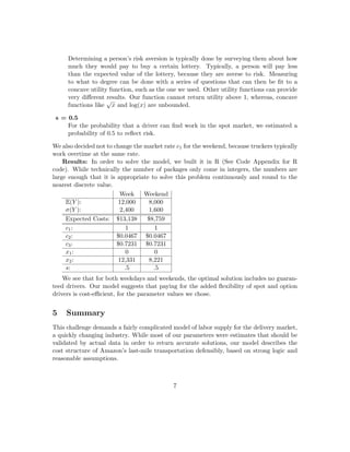
γ = 0.5
We found that γ = 0.5 returned reasonable figures for our units, so we used it for
simplicity’s sake. Determining γ empirically will be necessary for an accurate model:
6

7. Determining a person’s risk aversion is typically done by surveying them about how
much they would pay to buy a certain lottery. Typically, a person will pay less
than the expected value of the lottery, because they are averse to risk. Measuring
to what to degree can be done with a series of questions that can then be fit to a
concave utility function, such as the one we used. Other utility functions can provide
very different results. Our function cannot return utility above 1, whereas, concave
functions like
√
x and log(x) are unbounded.
s = 0.5
For the probability that a driver can find work in the spot market, we estimated a
probability of 0.5 to reflect risk.
We also decided not to change the market rate c1 for the weekend, because truckers typically
work overtime at the same rate.
Results: In order to solve the model, we built it in R (See Code Appendix for R
code). While technically the number of packages only come in integers, the numbers are
large enough that it is appropriate to solve this problem continuously and round to the
nearest discrete value.
Week Weekend
E(Y ): 12,000 8,000
σ(Y ): 2,400 1,600
Expected Costs: $13,138 $8,759
c1: 1 1
c2: $0.0467 $0.0467
c3: $0.7231 $0.7231
x1: 0 0
x2: 12,331 8,221
s: .5 .5
We see that for both weekdays and weekends, the optimal solution includes no guaran-
teed drivers. Our model suggests that paying for the added flexibility of spot and option
drivers is cost-efficient, for the parameter values we chose.
5 Summary
This challenge demands a fairly complicated model of labor supply for the delivery market,
a quickly changing industry. While most of our parameters were estimates that should be
validated by actual data in order to return accurate solutions, our model describes the
cost structure of Amazon’s last-mile transportation defensibly, based on strong logic and
reasonable assumptions.
7

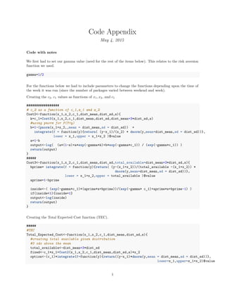
8. 6 Math Appendix: Mathematics of c2 and c3 worked out
Part 1: Math for equalizing option driver’s options (solve for c2)
u(c1) = [a · (1 − s) · u(c2) + a · (s) · u(c2 + c1 + c3) + b · u(c1 + c2)]
1 − e−c1
= [a · (1 − s) · (1 − e−c2
) + a · (s) · (1 − e−c2−c1−c3
) + b · (1 − e−c1−c2
)]
1 − e−c1
= a · (1 − s) − a · (1 − s)e−c2
+ a · (s) − a · (s) · e−c2−c1−c3
+ b − b · e−c1−c2
1 − e−c1
= a · (1 − s) + a · (s) + b − a · (1 − s)e−c2
− a · (s) · e−c2−c1−c3
− b · e−c1−c2
RHS: the first 3 terms sum to 1, so we can reduce both sides by 1:
−e−c1
= −a · (1 − s)e−c2
− a · (s) · e−c2−c1−c3
− b · e−c1−c2
e−c1
= a · (1 − s)e−c2
+ a · (s) · e−c2−c1−c3
+ b · e−c1−c2
e−c1
= a · (1 − s) + a · (s) · e−c1−c3
+ b · e−c1
· e−c2
e−c1
a · (1 − s) + a · (s) · e−c1−c3 + b · e−c1
= e−c2
⇒ c2 = ln
a · (1 − s) + a · (s) · e−c1−c3 + b · e−c1
e−c1
Part 2: Math for equalizing spot driver’s options (Solve for c3)
u(c1) = [a · s · u(c1 + c3) + b · u(c1 + c3)]
1 − e−c1
= [a · s · (1 − e−c1−c3
) + b · (1 − e−c1−c3
)]
1 − e−c1
= (a · s + b ) · (1 − e−c1
e−c3
)
1 − e−c1
= (a · s + b ) − (a · s + b ) · e−c1
e−c3
)
1 − e−c1
− a · s − b = −(a · s + b ) · e−c1
e−c3
)
⇒ c3 = ln
(a · s + b )e−c1
e−c1 + a · s + b − 1
8

9. Code Appendix
May 4, 2015
Code with notes
We first had to set our gamma value (need for the rest of the items below). This relates to the risk aversion
function we used.
gamma=1/2
For the functions below we had to include parameters to change the functions depending upon the time of
the week it was run (since the number of packages varied between weekend and week).
Creating the c2, c1 values as functions of x1, x2, and c1
#################
# c_2 as a function of c_1,x_1 and x_2
Cost2<-function(x_1,x_2,c_1,dist_mean,dist_sd,s){
k=c_1+Cost3(x_1,x_2,c_1,dist_mean,dist_sd,dist_mean+3*dist_sd,s)
#using pnorm for P(Y<y)
b=1-(pnorm(x_1+x_2,,mean = dist_mean,sd = dist_sd)) +
integrate(f = function(y){return( (y-x_1)/(x_2) * dnorm(y,mean=dist_mean,sd = dist_sd))},
lower = x_1,upper = x_1+x_2 )$value
a=1-b
output<-log( (a*(1-s)+a*exp(-gamma*k)+b*exp(-gamma*c_1)) / (exp(-gamma*c_1)) )
return(output)
}
#####
Cost3<-function(x_1,x_2,c_1,dist_mean,dist_sd,total_available=dist_mean+3*dist_sd,s){
bprime= integrate(f = function(y){return( (y-(x_1+x_2))/(total_available -(x_1+x_2)) *
dnorm(y,mean=dist_mean,sd = dist_sd))},
lower = x_1+x_2,upper = total_available )$value
aprime=1-bprime
inside<-( (exp(-gamma*c_1)*(aprime*s+bprime))/(exp(-gamma* c_1)+aprime*s+bprime-1) )
if(inside<1){inside=1}
output<-log(inside)
return(output)
}
Creating the Total Expected Cost function (TEC).
#####
#TEC
Total_Expected_Cost<-function(x_1,x_2,c_1,dist_mean,dist_sd,s){
#creating total available given distribution
#3 sds above the mean
total_available<-dist_mean+3*dist_sd
fixed<-c_1*x_1+Cost2(x_1,x_2,c_1,dist_mean,dist_sd,s)*x_2
option<-(c_1)*integrate(f=function(y){return((y-x_1)*dnorm(y,mean = dist_mean,sd = dist_sd))},
lower=x_1,upper=x_1+x_2)$value
1

10. option2<-(c_1)*(x_1+x_2)*(1-pnorm(x_1+x_2,mean=dist_mean,sd=dist_sd))
spot<-(c_1+Cost3(x_1,x_2,c_1,dist_mean,dist_sd,total_available,s))*
integrate(f=function(y){return((y-x_1-x_2)*
dnorm(y,mean = dist_mean,sd = dist_sd) )},
lower = x_1+x_2 ,upper = total_available)$value
output<-(fixed+option+option2+spot)
return(output)
}
Before we go any further, we needed to set our s value (probability to find work on general spot market), and
the c1 value.
s_value=.5
c_value=1
Now, in preparation for optimizing the TEC, we made a second TEC function that just a function of 2
variables, which was fairly simple to optimize.
Total_Expected_Cost_Optimize<-function(xvalues){
return(Total_Expected_Cost(x_1=xvalues[1],x_2=xvalues[2],c_1=c_value,
dist_mean=12000,dist_sd = 2400,s=s_value))
}
Since the optimization function looks for local minima, the answer depends on the starting point. Below is
one such optimization sample starting point.
#Since the optimization function looks for local minima, the answer
# depends on the starting point. Here is one such optimization sample starting point.
data<-optim(c(2500,2500),fn=Total_Expected_Cost_Optimize,lower=c(0,0),method="L-BFGS-B")
and here is the report from the optimization function:
data
## $par
## [1] 0.00 12330.87
##
## $value
## [1] 13137.77
##
## $counts
## function gradient
## 26 26
##
## $convergence
## [1] 0
##
## $message
## [1] "CONVERGENCE: REL_REDUCTION_OF_F <= FACTR*EPSMCH"
2

11. To make sure we didn’t miss a lower local minimum (the global minimum), we decided to create a small grid
of potential plausible starting values.
fulldata<-matrix(0,nrow=3,ncol=3)
i=1
#######
#checking over multiple starting points
#basically checking starting points via grid approach
for(index1 in c(5000,7500,10000)){
j=1
for(index2 in c(5000,7500,10000)){
data<-optim(c(index1,index2),fn=Total_Expected_Cost_Optimize,lower=c(0,0),method="L-BFGS-B")
fulldata[i,j]<-data$value
j=j+1
}
i=i+1
}
It should be noted that some of the entries are zeros because the code gets errors. This is due to the fact
that we assumed that total available drivers was 19,200 for week days, which is less than the starting point
x1 = 10, 000 and x2 = 10, 000, it seems as if we found a good result anyway, even without a complete grid.
fulldata
## [,1] [,2] [,3]
## [1,] 13137.77 13137.77 13137.77
## [2,] 13137.77 13137.77 13137.77
## [3,] 13137.77 13137.77 13137.77
From the grid above we selected the optimal starting point and ran the model
#selecting minimum value from fulldata grid
data<-optim(c(5000,2500),fn=Total_Expected_Cost_Optimize,lower=c(0,0),method="L-BFGS-B")
And below is all the data from our predicted best model
#print out values
data
## $par
## [1] 0.00 12330.89
##
## $value
## [1] 13137.77
##
## $counts
## function gradient
## 25 25
##
## $convergence
3

12. ## [1] 0
##
## $message
## [1] "CONVERGENCE: REL_REDUCTION_OF_F <= FACTR*EPSMCH"
#checking results
Total_Expected_Cost_Optimize(data$par)
## [1] 13137.77
#getting C_2 value
Cost2(x_1=data$par[1],x_2=data$par[2],c_1=c_value,dist_mean=12000,dist_sd = 2400,s=s_value)
## [1] 0.0467159
#getting C_3 value
Cost3(x_1 =data$par[1],x_2=data$par[2],c_1=c_value,dist_mean=12000,dist_sd = 2400,s=s_value)
## [1] 0.7231073
#re-examing s and c_1 values
s_value
## [1] 0.5
#c_1 value
c_value
## [1] 1
Weekend
The above optimum was just for the week, so below is the code for the weekend (no additional commentary)-
we just changed the distibution function.
#Weekends
########
Total_Expected_Cost_Optimize<-function(xvalues){
return(Total_Expected_Cost(x_1=xvalues[1],x_2=xvalues[2],
c_1=c_value,dist_mean=8000,dist_sd = 1600,s=s_value))
}
#Since the optimization function looks for local minima, the answer
# depends on the starting point. Here is one such optimization sample starting point.
data<-optim(c(5000,2500),fn=Total_Expected_Cost_Optimize,lower=c(0,0),method="L-BFGS-B")
data
## $par
## [1] 0.000 8220.581
##
4

13. ## $value
## [1] 8758.515
##
## $counts
## function gradient
## 22 22
##
## $convergence
## [1] 0
##
## $message
## [1] "CONVERGENCE: REL_REDUCTION_OF_F <= FACTR*EPSMCH"
#We could grid to look at possiblities, but this value looks pretty good
Total_Expected_Cost_Optimize(data$par)
## [1] 8758.515
#getting C_2 value
Cost2(x_1=data$par[1],x_2=data$par[2],c_1=c_value,dist_mean=8000,dist_sd = 1600,s=s_value)
## [1] 0.04671558
#getting C_3 value
Cost3(x_1 =data$par[1],x_2=data$par[2],c_1=c_value,dist_mean=8000,dist_sd = 1600,s=s_value)
## [1] 0.7231052
#re-examing s and c_1 values
s_value
## [1] 0.5
#c_1 value
c_value
## [1] 1
5

14.
Multivariable Calculus
Probability
Structure and Interpretation
of Computer Programming
Deterministic Optimization
Python, Java, HTML5, CSS3, jQuery
COURSES & SKILLS
Linear Algebra
Statistics
Data Structures
Microeconomic Theory
Decision Analysis
Adobe Illustrator, Photoshop, InDesign
EXPERIENCE
Web Development Intern, Branch Metrics
• Built web pages for company site and partner landing pages
• Developed applications of deferred deeplinking technology
• Designed pitch decks for investors and sales decks for potential clients
• Wrote market analysis reports, copy, and promotional articles
Research Assistant, Gallant Lab
• Data processing of fMRI scans for predictive neuroimaging
• Worked with Pylab, Freesurfer and Blender software
Quality Improvement Intern, CA Correctional Health Care
• Quantitative research on usability and adoption of new technology
• Studied use of data visualization as quality and performance driver
• Researched compensation models and organizational efficiency
Summer 2014
Palo Alto, CA
Summer 2013
Berkeley, CA
Summer 2012
Sacramento, CA
UC Berkeley, Spring 2017
3.7 GPA
Operations Research & Management Science
Regents’ and Chancellor’s Scholar
Leadership Award Recipient
EDUCATION STUDENT LEADERSHIP
House Manager, BSC
Manages house budgets and assets
Professional Development Coordinator, RCSA
Organizes professional events and resources
for top 2% of Berkeley students
ABIGAIL CHAVER
1730 La Loma Ave | Berkeley CA, 94709 | 510-387-8125 | abigailchaver@berkeley.edu

15. Benjamin LeRoy
2227 Derby Street Apt 5 — Berkeley, CA 94705
Phone: (707) 328-0714 — E-Mail: benjaminleroy@berkeley.edu
Education
University of California, Berkeley Expected Graduation: December 2015
Bachelors Degree in Applied Mathematics GPA: 3.93/4.0
Bachelors Degree in Statistics
Relevant Coursework:, Stochastic Processes, Statistical Theory, Mathematical Microeconomics,
Courses in Progress: Machine Learning, Economic Demography
Santa Rosa Junior College (SRJC) Graduation: May 2013
Associate Degrees in Mathematics with Highest Honors, Economics with Highest Honors GPA: 3.89/4.0
Skills
Leadership Skills
• Guided executive committees for events in the Order of the Arrow (OA), Boy Scouts National
Honor Society, for 1500+ active members
• Managed development of classes, assembling trainers and running of large training events (40
classes serving 300+ members)
Analytic Skills
• Developed and collected surveys from Boy Scout training events and presented committees
with recommendations on the direction for future years
• Developed budget plans for a $30,000 non-profit, and advised executive committees on
budget matters
• Identified the need and wrote up Mathematica guides to help SRJC Math Lab tutors assist
Calculus students with Mathematica programming
• Initiated redevelopment of training program for new hires in the Front End department at
Oliver’s Market for 10-15 people per year at my store
Team-Oriented Skills
• Boy Scout committees, from a local (city) to sectional level(multi- state), brainstorming for big
events, develop programs, and worked on restructuring the sectional organization in 2009.
• Served on Staff as a table guide at two OA National Leadership Seminars and assisted trainers
in presentation prep and developing follow up discussions for table (6-8 individuals)
• Collaborated on large coding projects in Stat 133
Employment History
Math Tutor, Computer and Mathematics Lab, Santa Rosa Junior College, Santa Rosa, CA 8/11 -5/13
Calculus and Linear Algebra Courses Grader, Santa Rosa Junior College, Santa Rosa, CA 8/12 – 5/13
Cashier and Clerk, Oliver’s Market, Montecito, Santa Rosa, CA 5/09 – 8/13*
Volunteer History Highlight
Active Member, Cal Habitat for Humanities 1/14-Present
Training Adviser (2012), Training Coordinator (2011), Section Chief (2010), Section W3N,
Order of the Arrow, Boy Scout of America, Northern California 6/06-5/12
Other
Technical Skills: R (in use in 2 current classes as well), Python, Microsoft Office, Basic Matlab
Awards:
• Vigil Member, Boy Scouts of America’s Honor Society (December 2008)
• Eagle Scout, Boy Scouts of America (November 2006)
Scholarships:
• Robert F Argella Scholarship, SRJC Mathematics Scholarship (May 2013)
• John M Soares Memorial Economics Scholarship (May 2013)
• Cal Alumni Club of Oakmont Transfer Scholarship (May 2013)