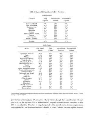
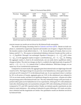
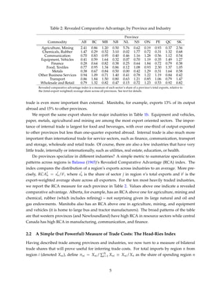
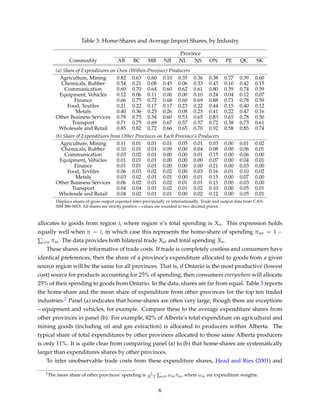
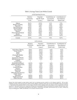
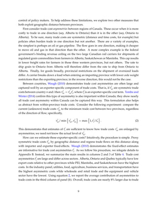
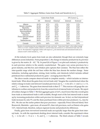
This document analyzes internal trade costs in Canada using detailed trade and output data. It finds: 1) Internal trade accounts for around 11% of Canadian output on average and is as important as international trade for some provinces. 2) Estimated internal trade costs are large (8-15% of trade value) and vary significantly across sectors and provinces, with poorer regions generally facing higher costs. 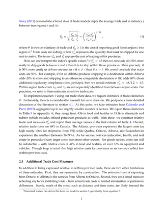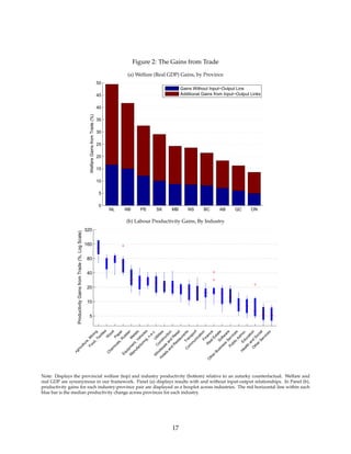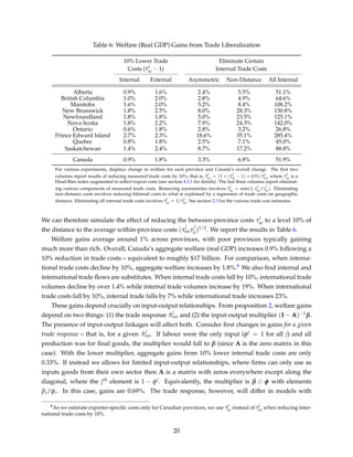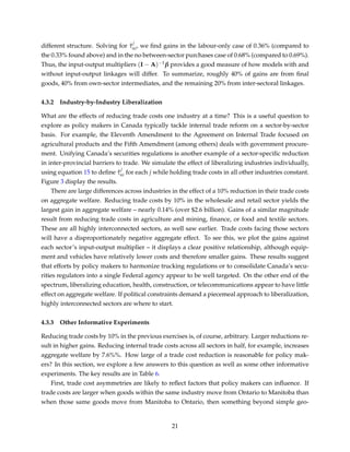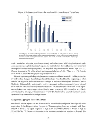3) Reducing internal trade costs by liberalizing sectors could significantly increase Canada's GDP and welfare, with gains estimated between $50-130 billion or 3-7% of GDP depending on the policy experiment. Highly interconnected industries have the largest gains from liberalization.

1. Internal Trade, Productivity, and Interconnected Industries:
A Quantitative Analysis
Lukas Albrecht Trevor Tombe
This Version: May 2015
Abstract
Does trade within a country affect welfare and productivity? What are the magnitude and
consequences of costs to such trade? To answer these questions, we exploit unique Canadian
data to measure internal trade costs in a variety of ways – they are large, and vary across sectors
and provinces. To quantify their consequences for welfare and productivity, we use a recent
multi-sector trade model featuring rich input-output relationships. We find inter-provincial
trade is an important contributor to Canada’s GDP and welfare, though there are significant
costs to such trade. Reducing inter-provincial trade costs by 10% yields aggregate gains of
0.9%; eliminating our preferred estimates of costs, gains average between 3-7% – equivalent to
real GDP gains between $50-$130 billion. Finally, as policy reforms are often sector-specific, we
liberalize sectors one at a time and find gains are largest in highly interconnected industries.
JEL Classification: F1, F4, R1
Keywords: Internal trade; gains from trade; input-output linkages
Tombe (Corresponding Author): Assistant Professor, Department of Economics, University of Calgary, 2500 University Drive NW,
Calgary, Alberta, T2N1N4. Email: ttombe@ucalgary.ca. Phone: 1-403-220-8068. Albrecht: Former MA student at the University of
Calgary, now a Regulatory Analyst with Canadian Pacific Railway Ltd. Email: Lukas_Albrecht@cpr.ca. We thank Jennifer Winter for
valuable comments and suggestions. Tombe acknowledges generous financial support provided by the Social Science and Humanities
Research Council (IDG 430-2012-421).

2. 1 Introduction
Is it more costly to trade across a provincial boundary than it is to trade within a province? If so,
what effect do such costs have on aggregate welfare (real GDP) or industry productivity? Unlike
barriers to international trade, the effect of barriers to trade within countries is only beginning to
receive significant attention – largely due to recent theoretical advances and the availability of
high-quality data on inter-provincial trade (hereafter, internal trade). In this paper, we quantify
the magnitude and consequences of internal trade costs across a variety of sectors and identify the
most valuable sectors for policy makers to reform. This is relevant, as efforts to reduce internal
trade costs are often sector-specific – especially in Canada. Our analysis exploits uniquely detailed
data from Canada on internal trade and a recent multi-sector trade model featuring rich input-
output relationships (Caliendo and Parro, 2015). We find internal trade costs are large, vary across
sectors and provinces, and reduce productivity and welfare. They also interact with input-output
relationships – liberalizing highly interconnected industries yields the largest gains.
What are internal trade costs? Of course, explicit tariffs do not exist, but a wide variety of reg-
ulatory restrictions on the movement of goods and services can have substantial effects on trade.
While Beaulieu et al. (2003) give an excellent summary, let us provide some examples. Provin-
cial licensing requirements for stock brokers, accountants, lawyers, and other professions, prevent
customers in one province from hiring providers registered in another. Different regulations be-
tween provinces, for long-haul freight transportation or product safety standards, for example,
also increase costs of trade between provinces. Biased government procurement policies, where
governments and agencies give preferences to within-province suppliers, are also trade costs.
These measures, and more, suggest there is scope for internal liberalization – a fact recognized
by Canadian policy makers and politicians (Ivison, 2014).
We use a variety of techniques to estimate internal trade costs, starting with the Head-Ries
index of trade restrictiveness (Head and Ries, 2001; Novy, 2013). We leave the details behind this
measure to the next section, but a brief intuitive description is useful here. The index infers trade
costs, which are not observable, from provincial production and trade flows, which are. Essen-
tially, trade costs generate systematic tendencies among provinces to allocate more spending to
their own producers, rather than producers in other provinces. The index, however, infers trade
costs relative to costs of trading within provinces (say, between Calgary and Edmonton). In addition,
it does not isolate policy-relevant costs from other factors such as distance. To address these lim-
itations, we explore two other measures. First, trade costs may be higher in one direction of flow
(say, from Alberta to Ontario) than in the other (Ontario to Alberta). This asymmetry in trade costs
is an important feature of both international trade (Waugh, 2010) and internal trade (Tombe and
Winter, 2014). They likely better reflect policy-relevant costs and are not valued relative to within-
province costs. We identify these asymmetries as in the literature and find they are large, adding
nearly 8% to average internal trade costs. Our second measure supposes the primary driver of
trade costs unrelated to policy is physical distance. As the Head-Ries index describes average
between-province trade costs relative to within-province trade costs, we essentially regress the
1

3. index on a measure of distance between provinces relative to within-province distances (between
cities). The residuals from this regression may be informative of policy-relevant trade costs. On
average, these non-distance costs add 15% to average internal trade costs. With both measures,
we find poor regions tend to face the highest internal trade costs.
What are the consequences of these internal trade costs on productivity and welfare in Canada?
To answer this question, we use a recent model featuring multiple interconnected industries de-
veloped by Caliendo and Parro (2015). When solved using the “Exact-Hat Algebra” of Dekle et
al. (2007), the model is a highly tractable quantitative tool for evaluating trade policy. While we
postpone a more detailed discussion to section 3, it is straightforward to see why interconnections
between multiple industries matters. With input-output links, changes to one sector affect many
others since the output of one is an input for another. Gains from trade are therefore amplified
by each sector’s “influence” on the aggregate economy. A summary measure of this influence is
found in many literatures: the vector of TFP Multipliers in Jones (2013), the Influence Vector in
Acemoglu et al. (2012) and Carvalho and Gabaix (2013), or (more loosely) the vector of Sales/GDP
ratios in Hulten (1978). We derive an analogous measure in proposition 2 and demonstrate trade
and trade costs matter more in more “influential” sectors. Sectors with large input-output multi-
pliers tend to have (1) large internal trade flows and (2) large gains from trade liberalization.
With the model, we perform a variety of quantitative experiments. We first ask: Who gains
from trade in Canada? This is a common experiment in the international trade literature and in-
volves comparing initial welfare to the counterfactual level of welfare when trade is prohibited.
We find aggregate welfare is 18.3% higher than in autarky. Compared to the case of no inter-
provincial trade, but allowing for international trade, aggregate welfare is 4.4% higher. For inter-
nal trade costs, reducing them by 10% increases aggregate welfare by roughly 0.9% (equivalent to
a real GDP increase of $17 billion). Eliminating trade cost asymmetries, aggregate gains are over
3%; removing trade costs unrelated to distance, gains are nearly 7%. These estimates suggest re-
ducing internal trade barriers could add $50-$130 billion to Canada’s GDP. If inter-provincial trade
costs were completely eliminated, an implausible but illustrative experiment, aggregate gains for
Canada exceed 50%. Moreover, we consistently find poor regions gain more from liberalization
than rich regions.
In addition to aggregate outcomes, we explore a variety of industry-specific results, as pol-
icy reforms are often piecemeal. A 10% reduction in internal trade costs for the agriculture and
mining sector increases aggregate welfare by 0.1%. Other important sectors include food, textiles,
wholesale and retail trade, and finance – all with gains around 0.1% for a 10% reduction of their
trade costs. The gains from sector-specific liberalizations are closely related to input-output links
– highly interconnected industries, as measured by a sector’s “influence”, have the largest gains
from trade liberalization. We already know from Caliendo and Parro (2015) and Costinot and
Rodriguez-Clare (2014) that inter-sectoral linkages are key for aggregate gains from trade – typi-
cally more than doubling gains from trade. Our sector-specific liberalizations build on that result
to identify key sectors for reform.
2

4. Our work fits within a recent and growing literature, measuring the magnitude and effect of
internal barriers to trade. Typically, work in this area exploits gravity-based empirical approaches
to measure internal trade costs for a variety of countries, from the United States (Wolf, 2000; Hill-
berry and Hummels, 2003; Yilmazkuday, 2012) and the European Union (Nitsch, 2000; Chen, 2004)
to China (Poncet, 2005). For Canada, Anderson and Yotov (2010) investigate the nature and con-
sequences of internal trade costs, though their main focus is on who pays for trade costs (its inci-
dence). They also simulate potential gains from trade cost reductions and find poor regions stand
to gain more than rich – a result we confirm. Finally, the two most closely related papers in this
literature are Agnosteva, Anderson and Yotov (2014) and Tombe and Winter (2014). Tombe and
Winter (2014) take an aggregate approach to measure internal trade costs in Canada, the United
States, and China and focus on the interaction of trade costs with federal tax and transfer systems.
Agnosteva, Anderson and Yotov (2014) develop a novel approach to estimate policy-relevant in-
ternal trade costs, even by sector and within provinces, although they do not quantify the effect of
trade or trade costs on productivity and welfare. Our work complements theirs.
Overall, our purpose is neither to provide theoretical nor empirical innovations; instead, we
use high-quality and detailed data with frontier methods from the international trade literature
(Head and Ries, 2001; Waugh, 2010; Caliendo and Parro, 2015) to increase understanding of the
magnitude and consequences of internal trade costs at the sector level. This is an active and
important policy area, especially for Canada.
2 Canadian Internal Trade and Its Costs
This section examines in detail the nature and composition of Canada’s internal trade, especially
how it varies by province and sector. The data for our analysis are uniquely detailed. Statistics
Canada provides high quality province and commodity-level trade data, both within Canada and
with the rest of the world (captured as a single entity).1 We aggregate commodities into industries
based on OECD-STAN data, combining sectors where necessary to ensure positive production in
each province and sector. Details are in Appendix A.
2.1 Export Orientation of Provinces and Industries
Table 1a displays each province’s share of output exported. Overall, just over one-quarter of
production is exported. Province vary: Newfoundland and Labrador, Saskatchewan, and New
Brunswick all export more than a third of their output while Nova Scotia and British Columbia
export less than a quarter of theirs. Internal trade is almost as important as international trade.
Comparing columns two and three of Table 1a, we find roughly 60% of all goods exported from a
1Statistics Canada infers inter-provincial trade from a variety of sources such that provincial supply and demand
constraints (from Provincial IO Tables) are respected. Goods trade is largely based on shipment information from the
Annual Survey of Manufacturers and the Wholesale Origin and Destination Survey. Services trade, however, faces
greater difficulties; for example, there is no source of bilateral trade in financial services and Statistics Canada imputes
trade with a number of ad-hoc approaches. For further detail, see Généreux and Langen (2002).
3

5. Table 1: Share of Output Exported, by Province
(a) By Province
Province Total
Exports
International
Exports
Intranational
Exports
Newfoundland 36% 20% 16%
New Brunswick 34% 19% 15%
Saskatchewan 34% 22% 12%
Alberta 28% 16% 12%
Manitoba 28% 13% 15%
Ontario 25% 16% 9%
Prince Edward Island 25% 11% 14%
Quebec 24% 13% 11%
Nova Scotia 22% 10% 12%
British Columbia 21% 11% 10%
Average 26% 15% 11%
(b) By Sector
Sector ISIC (Rev3)
Codes
Total
Exports
International
Exports
Intranational
Exports
Equipment, Vehicles 29-35 77% 66% 11%
Paper 21-22 64% 45% 19%
Metals 26-28 60% 45% 15%
Agriculture, Mining 01-14 59% 41% 18%
Food, Textiles 15-19 58% 23% 35%
Chemicals, Rubber 23-25 55% 35% 21%
Manufacturing, n.e.c. 36-37 53% 33% 20%
Wood 20 53% 32% 21%
Transport 60-63 31% 14% 17%
Other Business Services 73-74 26% 11% 14%
Hotels and Restaurants 55 24% 11% 13%
Communication 64 24% 7% 16%
Wholesale and Retail 50-52 23% 10% 13%
Finance 65-67 20% 4% 16%
Software 72 18% 8% 10%
Other Services 90-93 9% 2% 7%
Utilities 40-41 5% 4% 1%
Real Estate 70-71 4% 1% 2%
Education 80 3% 2% 1%
Health and Social 85 1% 0% 1%
Public Admin. 75 0% 0% 0%
Construction 45 0% 0% 0%
Displays shares of gross output exported inter-provincially or internationally. Trade and output data from CANSIM 386-0003. Overall
average is output-weighted.
province are sent abroad and 40% are sent to other provinces, though there are differences between
provinces. At the high end, 22% of Saskatchewan’s output is exported abroad compared to only
10% of Nova Scotia’s. The share of output exported within Canada varies less across provinces,
ranging from 16% for Newfoundland and Labrador to 9% for Ontario. For some regions, internal
4

6. Table 2: Revealed Comparative Advantage, by Province and Industry
Province
Commodity AB BC MB NB NL NS ON PE QC SK
Agriculture, Mining 2.41 0.86 1.20 0.50 5.76 0.62 0.19 0.93 0.37 2.56
Chemicals, Rubber 1.47 0.29 0.52 3.10 0.02 1.77 0.72 0.31 1.32 0.68
Communication 0.70 0.83 0.95 0.40 0.46 1.16 1.28 0.56 1.12 0.54
Equipment, Vehicles 0.41 0.59 1.64 0.32 0.07 0.70 1.19 0.35 1.49 1.27
Finance 0.28 0.64 0.82 0.38 0.25 0.64 1.84 0.72 0.79 0.38
Food, Textiles 0.77 0.95 1.34 0.86 0.12 1.08 0.93 2.30 1.37 1.05
Metals 0.38 0.67 0.84 0.50 0.00 0.42 1.29 0.31 1.64 0.58
Other Business Services 0.94 1.09 0.71 1.40 0.41 0.78 1.22 1.19 0.84 0.42
Transport 0.86 1.84 1.50 0.80 0.63 1.21 0.85 1.06 0.79 1.47
Wholesale and Retail 0.79 1.32 0.82 0.47 0.15 0.72 1.23 0.53 0.92 0.82
Revealed comparative advantage index is a measure of each sector’s share of a province’s total exports, relative to
the (total-export weighted) average share across all provinces. See text for details.
trade is even more important than external. Manitoba, for example, exports 13% of its output
abroad and 15% to other provinces.
We report the same export shares for major industries in Table 1b. Equipment and vehicles,
paper, metals, agricultural and mining are among the most export oriented sectors. The impor-
tance of internal trade is largest for food and beverages, with over one-third of output exported
to other provinces but less than one-quarter exported abroad. Internal trade is also much more
important than international trade for service sectors, such as finance, communication, transport
and storage, wholesale and retail trade. Of course, there are also a few industries that have very
little trade, internally or internationally, such as utilities, real estate, education, or health.
Do provinces specialize in different industries? A simple metric to summarize specialization
patterns across regions is Balassa (1965)’s Revealed Comparative Advantage (RCA) index. The
index compares the distribution of a region’s exports across industries to an average. More pre-
cisely, RCA
j
n = s
j
n/¯sj, where s
j
n is the share of sector j in region n’s total exports and ¯sj is the
export-weighted average share across all exporters. For the ten most heavily traded industries,
we report the RCA measure for each province in Table 2. Values above one indicate a revealed
comparative advantage. Alberta, for example, has an RCA above one for agriculture, mining and
chemical, rubber (which includes refining) – not surprising given its large natural and oil and
gas endowments. Manitoba also has an RCA above one in agriculture, mining, and equipment
and vehicles (it is home to large bus and tractor manufacturers). The broad patterns of the table
are that western provinces (and Newfoundland) have high RCA in resource sectors while central
Canada has high RCA in manufacturing, communication, and finance.
2.2 A Simple (but Powerful) Measure of Trade Costs: The Head-Ries Index
Having described trade among provinces and industries, we now turn to a measure of bilateral
trade shares that will prove useful for inferring trade costs. For total imports by region n from
region i (denoted Xni), define πni = Xni/ ∑N
i=1 Xni ≡ Xni/Xn as the share of spending region n
5

7. Table 3: Home-Shares and Average Import Shares, by Industry
Province
Commodity AB BC MB NB NL NS ON PE QC SK
(a) Share of Expenditures on Own (Within-Province) Producers
Agriculture, Mining 0.82 0.63 0.60 0.10 0.35 0.36 0.38 0.77 0.39 0.60
Chemicals, Rubber 0.54 0.21 0.08 0.45 0.06 0.33 0.43 0.10 0.42 0.15
Communication 0.69 0.70 0.64 0.60 0.62 0.61 0.80 0.59 0.74 0.59
Equipment, Vehicles 0.12 0.06 0.11 0.00 0.00 0.10 0.24 0.04 0.12 0.07
Finance 0.66 0.75 0.72 0.68 0.60 0.69 0.88 0.71 0.78 0.59
Food, Textiles 0.21 0.22 0.17 0.17 0.23 0.22 0.44 0.15 0.40 0.12
Metals 0.40 0.36 0.25 0.26 0.08 0.23 0.41 0.22 0.47 0.16
Other Business Services 0.78 0.75 0.54 0.60 0.53 0.65 0.83 0.65 0.78 0.50
Transport 0.71 0.75 0.69 0.67 0.57 0.57 0.72 0.38 0.73 0.61
Wholesale and Retail 0.85 0.82 0.72 0.66 0.65 0.70 0.92 0.58 0.85 0.74
(b) Share of Expenditures from Other Provinces on Each Province’s Producers
Agriculture, Mining 0.11 0.01 0.01 0.01 0.05 0.01 0.03 0.00 0.01 0.02
Chemicals, Rubber 0.10 0.01 0.01 0.09 0.00 0.04 0.08 0.00 0.06 0.01
Communication 0.03 0.02 0.01 0.00 0.00 0.01 0.15 0.00 0.06 0.00
Equipment, Vehicles 0.01 0.01 0.01 0.00 0.00 0.00 0.07 0.00 0.04 0.01
Finance 0.01 0.01 0.01 0.00 0.00 0.00 0.21 0.00 0.03 0.00
Food, Textiles 0.06 0.03 0.02 0.02 0.00 0.03 0.16 0.01 0.10 0.02
Metals 0.03 0.02 0.01 0.01 0.00 0.01 0.15 0.00 0.07 0.00
Other Business Services 0.06 0.02 0.01 0.02 0.01 0.01 0.13 0.00 0.03 0.00
Transport 0.04 0.04 0.01 0.02 0.01 0.02 0.10 0.00 0.05 0.01
Wholesale and Retail 0.04 0.02 0.01 0.01 0.00 0.02 0.12 0.00 0.05 0.01
Displays shares of gross output exported inter-provincially or internationally. Trade and output data from CAN-
SIM 386-0003. All shares are strictly positive – values are rounded to two decimal places.
allocates to goods from region i, where region n’s total spending is Xn. This expression holds
equally well when n = i, in which case this represents the home-share of spending πnn = 1 −
∑i=n πni. The data provides both bilateral trade Xni and total spending Xn.
These shares are informative of trade costs. If trade is completely costless and consumers have
identical preferences, then the share of a province’s expenditure allocated to goods from a given
source region will be the same for all provinces. That is, if Ontario is the most productive (lowest
cost) source for products accounting for 25% of spending, then consumers everywhere will allocate
25% of their spending to goods from Ontario. In the data, shares are far from equal. Table 3 reports
the home-share and the mean share of expenditure from other provinces for the top ten traded
industries.2 Panel (a) indicates that home-shares are often very large; though there are exceptions
– equipment and vehicles, for example. Compare these to the average expenditure shares from
other provinces in panel (b). For example, 82% of Alberta’s total expenditure on agricultural and
mining goods (including oil and gas extraction) is allocated to producers within Alberta. The
typical share of total expenditures by other provinces allocated to those same Alberta producers
is only 11%. It is quite clear from comparing panel (a) to (b) that home-shares are systematically
larger than expenditures shares by other provinces.
To infer unobservable trade costs from these expenditure shares, Head and Ries (2001) and
2The mean share of other provinces’ spending is 1
N−1 ∑n=i ωniπni, where ωni are expenditure weights.
6

8. Novy (2013) demonstrate a broad class of trade models imply the average trade cost in industry j
between two regions n and i is
¯τ
j
ni ≡
τ
j
ni
τ
j
nn
τ
j
in
τ
j
ii
=
π
j
nnπ
j
ii
π
j
niπ
j
in
1/2θj
, (1)
where θj is the cost-elasticity of trade and τ
j
ni ≥ 1 is the cost of importing good j from region i into
region n.3 Trade costs are iceberg, where τ
j
ni represents the quantity that must be shipped for one
unit to arrive. The terms τ
j
nn and τ
j
ii capture the cost of trading within provinces.
How can one interpret the index’s specific values? If ¯τ
j
ni = 1.5 then we conclude it is 50% more
costly to ship goods between n and i than it is to ship within those provinces. More precisely, it
is 50% more costly to deliver one unit to n if n = i than if n = i. We cannot conclude that trade
costs are 50%. For example, if for an Alberta producer shipping to a destination within Alberta
adds 20% to costs and shipping to an otherwise comparable destination in BC adds 80% (from
additional regulatory compliance costs, perhaps), then we would estimate ¯τ
j
ni = 1.8/1.2 = 1.5.
Within-region trade costs τnn and τii are not separately identified from between region costs. For
precision, we refer to these estimates as relative trade costs.
To implement equation 1 using our trade share data, we require estimates of trade elasticities
θj. Fortunately, there is a considerable research for us to draw on. We postpone a more detailed
discussion of the literature to section 4.1. At this point, we take estimates from Caliendo and
Parro (2015), aggregated up to our slightly smaller number of sectors. We report these elasticities
in Table 9 in Appendix A; they range from 4.56 in food and textiles to 19.16 in chemicals and
rubber (which includes refined petroleum products as well). With these, we construct relative
trade cost measures ¯τ
j
ni and report their average values in the first column of Table 4. Overall,
relative trade costs are 68% in Canada. The Atlantic provinces experience the largest costs (as
high nearly 106% for shipments from PEI) while Quebec, Ontario, Alberta, and Saskatchewan
experience the smallest (between 56-74%). As for sectors, services (education, health, and real
estate in particular) have larger costs than most other sectors. For goods sectors, costs can still
be substantial – with relative costs of 42% in food and textiles, or over 37% in equipment and
vehicles. Though keep in mind that high relative costs for provinces or sectors may reflect low
within-province costs.
2.3 Additional Trade Cost Measures
In addition to being expressed relative to within-province costs, there are two other limitations
of these estimates. First, they are symmetric by construction. The estimated cost of exporting
from Ontario to Alberta is the same as from Alberta to Ontario. Second, they are a broad measure
reflecting any factor inhibiting trade – from actual trade costs to limited information or preference
differences. Surely, much of the costs, such as distance and time costs, are likely beyond the
3Interested readers can derive this from our model in section 3; specifically, from equation 7.
7

9. Table 4: Average Trade Costs Within Canada
(a) By Exporting Province
Relative
Symmetric
Costs
Exporter-
Specific Trade
Costs t
j
i
Contribution of
Asymmetric
Trade Costs
Contribution of
Non-Distance
Trade Costs
Alberta 56.1% -15.5% 4.1% 7.2%
British Columbia 78.5% -11.4% 6.0% 10.5%
Manitoba 74.0% -4.8% 11.9% 9.8%
New Brunswick 66.4% 7.3% 16.4% 24.4%
Newfoundland 47.4% -6.8% 14.4% 3.2%
Nova Scotia 85.4% 14.3% 19.0% 31.5%
Ontario 73.5% -15.8% 1.3% 17.1%
Prince Edward Island 106.1% 22.2% 30.3% 32.1%
Quebec 62.5% -1.4% 13.4% 17.4%
Saskatchewan 62.8% 11.9% 34.1% 14.3%
Canada 67.8% 0.0% 7.8% 14.5%
(b) By Industry
Relative
Symmetric
Costs
Exporter-
Specific Trade
Costs t
j
i
Contribution of
Asymmetric
Trade Costs
Contribution of
Non-Distance
Trade Costs
Agriculture, Mining 24.4% -25.7% 6.3% -8.3%
Food, Textiles 42.0% -21.0% 5.8% -4.4%
Wood 24.9% -14.4% 2.1% 3.6%
Paper 25.7% -17.8% 3.4% 0.6%
Chemicals, Rubber 12.5% -16.7% 1.9% 1.6%
Metals 63.2% -2.8% 9.8% 11.8%
Equipment, Vehicles 37.4% -17.0% 4.3% 3.1%
Manufacturing, n.e.c. 60.2% -9.5% 4.8% 9.2%
Utilities – – – –
Construction – – – –
Wholesale and Retail 101.9% -14.8% 6.6% 14.8%
Hotels and Restaurants 97.0% 3.4% 9.8% 29.4%
Transport 83.5% -8.6% 10.8% 16.9%
Communication 84.8% 19.6% 12.2% 55.3%
Finance 91.7% -5.0% 12.4% 36.2%
Real Estate 192.4% 8.4% 12.1% 57.8%
Software 132.3% 18.4% 19.7% 54.6%
Other Business Services 90.6% -7.4% 8.1% 18.7%
Public Admin. – – – –
Education 230.0% 66.5% 15.5% 105.3%
Health and Social 245.8% 40.1% 16.7% 82.8%
Other Services 134.0% 17.1% 10.7% 44.5%
Reports the trade-weighted average relative trade cost, by exporting province (panel a) or by industry (panel b). All are trade-
weighted averages across province pairs within Canada. Relative symmetric trade costs are from the Head-Ries Index (see equation
1. Asymmetric costs reported relative to the average. The third column displays trade costs relative to the no-asymmetry case (see
equation 2). The fourth column uses a regression of trade costs on geographic distance (normalized by average within-province costs;
that is, dni/
√
dnndii), with exporter and importer fixed effects. Construction and public administration have no trade. Utilities has
only two trading pairs: AB-BC and NB-PEI, so we exclude it from the results.
8

10. control of policy makers. To help address these limitations, we explore two other measures that
both exploit geographic distance between provinces.
First consider trade cost asymmetries between regions of Canada. These occur when it is more
costly to trade in one direction (say, Alberta to Ontario) than it is in the other (say, Ontario to
Alberta). To be sure, many trade costs are symmetric (distance and time costs, for example) but
policies often burden trade in one direction but not another. There are a variety of examples,
the simplest is perhaps an oil or gas pipeline. The flow goes in one direction, making it cheaper
to move oil and gas in that direction than the other. A more complex example is the federal
government’s binding revenue ceiling on the two large Canadian rail carriers for shipments of
regulated grain commodities from farmers in Alberta, Saskatchewan or Manitoba. This cap results
in lower freight rates for farmers in those three western provinces, but not others. The rate to
ship grain to Ontario from Alberta will therefore differ from the rate to ship from Ontario to
Alberta. Finally, for goods broadly, provincial restrictions on the shipment of oversized loads
differ. A carrier breaks down a load when entering an importing province with lower axle weight
restrictions than the exporting province; in the reverse direction, this would not be the case.
Between countries, Waugh (2010) demonstrates trade cost asymmetries are often large and
captured well by an exporter-specific component of trade costs. That is, if t
j
ni are symmetric trade
costs between country n and i then τ
j
ni = t
j
nit
j
i, where t
j
i is an exporter-specific cost term. Tombe and
Winter (2014) confirm this type of asymmetry is also important within Canada; they show nearly
all trade cost asymmetry within Canada can be captured this way. This formulation also helps
us abstract from within-province trade costs. Consider the following experiment: compare the
current (unknown) trade costs τ
j
ni to the minimum trade cost between two provinces, regardless
of the direction of flow; specifically,
τ
j
ni/ min τ
j
ni, τ
j
in = max 1, t
j
i/t
j
n . (2)
This demonstrates that estimates of t
j
i are sufficient to know how trade costs τ
j
ni are enlarged by
asymmetries; we need not know the actual level of τ
j
ni.
How can we estimate these exporter-specific costs? Intuitively, the procedure is simple. Proxy
symmetric trade costs t
j
ni by geographic distance and regress trade flows on this distance along
with importer and exporter fixed-effects. Waugh (2010) demonstrates the fixed-effect estimates
are informative for trade cost asymmetries t
j
i. As we follow his procedure, we relegate details to
Appendix B. Instead, we summarize the main results in columns 2 and 3 of Table 4. Trade cost
asymmetries t
j
i are large and differ across sectors. Alberta, Ontario and Quebec typically have low
export costs relative to other provinces while PEI, Manitoba, and Saskatchewan have the highest
costs. In the industry panel, utilities, food, agriculture, business services, and transportation have
the highest asymmetric costs while wholesale and retail trade and the equipment and vehicle
sector have the lowest. Using equation 2, we report the average contribution of asymmetries to
trade costs in the third column of panel (b). Overall, trade costs are nearly 8% larger due to trade
9

11. cost asymmetries. While this is small relative to the value for ¯τ
j
ni, we will later show even these
small trade costs can have substantial effects on productivity and welfare.
Our second approach to isolate more policy-relevant costs also uses geographic distance. If
trade costs are τni = tniti then from equation 1 it is easy to show ¯τ
j
ni = ¯t
j
ni(t
j
it
j
n)1/2, where ¯t
j
ni =
(t
j
nit
j
in/τ
j
nnτ
j
ii)1/2. As before, we proxy the average symmetric relative trade costs ¯t
j
ni with geo-
graphic distance ¯dni = dni/
√
dnndii, which is the between-province distance relative to the av-
erage within-province distance (see Appendix B for details). To purge ¯τ
j
ni of variation related to
geographic distance, estimate
ln( ¯τ
j
ni) = δj
ln( ¯dni) + ι
j
n + η
j
i +
j
ni.
We report the results of this regression for each industry in Table 11 of Appendix B. The distance-
elasticity of trade costs vary by sector, but are typically around 0.20. Trade costs unexplained by
geographic distance are ( ¯τ
j
ni/ ¯d
ˆδj
ni) − 1. We refer to these as “non-distance trade costs”, the average
of which are in the fourth columns of Table 4. Distance explains much, though non-distance costs
amplify overall relative trade costs in Canada by 15%.4
2.4 Trade and Input-Output Linkages
Input-output linkages between sectors will mean trade costs facing one industry cascade through-
out the economy. After all, industries are not isolated from one another – output from one is used
as inputs by others.
Are input-output linkages and trade related? To answer this question, consider the summary
measure of a sector’s “influence” discussed briefly in the introduction. Acemoglu et al. (2012),
Jones (2013), Carvalho and Gabaix (2013), and others, demonstrate the effect of sectoral produc-
tivity shocks on the aggregate economy are summarized by a vector input-output multipliers
(I − A)−1β, where (I − A)−1 is the classic J × J Leontief Inverse Matrix and β is a J × 1 vector of
final demand shares. In proposition 2, we show the same expression holds for magnifying gains
from trade. Using the OECD input-output data, we construct these multipliers in Appendix A;
here, we display their relationship to trade in Figure 1. Primary producers within the agriculture
and the mining and oil and gas sectors, along with producers in the chemicals, food, wholesale
and retail trade, equipment and vehicle sectors are all highly traded sectors with significant in-
fluence on the aggregate economy. There are some exceptions. Real estate, for example, is a very
important sector for aggregate GDP, but accounts for little internal trade. Overall, however, sectors
that dominate Canada’s internal trade systematically have higher input-output multipliers.5
4The negative trade costs for agriculture, mining are statistically different from zero, indicating distance more than
accounts for trade costs in this sector. For chemicals, rubber (which includes refined petroleum products) the negative
estimate is not different from zero.
5In Appendix A, we show sectors with high intermediate input shares also export a large share of output.
10

12. Figure 1: Internal Trade and Input-Output Multipliers
Agriculture, Mining
Food, Textiles
Chemicals, Rubber
Metals Equipment, Vehicles
Wholesale and Retail
Transport
Finance
Real Estate
Other Business Services
0.05.1.15
ShareofCanada’sInternalTrade(%)
0 .05 .1 .15 .2
Aggregate Input−Output Multiplier
Note: Displays each industry’s share of total internal trade in Canada against the industry’s Input-Output
Multiplier. This multiplier summarizes the “influence” of each sector on aggregate economic activity. This
multiplier is defined as in Jones (2013): (I − A)−1β, where (I − A)−1 is the standard Leontief Inverse
Matrix and β is a vector of final-demand shares (see text for details).
3 A Multi-Sector Model of Internal Trade
What are the consequences of internal trade costs for Canada’s income and productivity? To
answer this question, we must place more structure on the data using the Caliendo and Parro
(2015) model featuring multiple sectors and rich input-output relationships. There are N = 11
regions, representing the 10 provinces of Canada plus the rest of the world. There is a single
primary factor of production – say, labour. A sector’s output can be consumed as a final good by
a representative household in each region or used as an input into the production of other goods.
Each sector’s output is a composite of a continuum of tradable varieties, which are purchased from
the cheapest source. The productivity with which each region can produce each variety differs,
which is the basis for trade. With the broad setup in mind, let’s move onto the details.
3.1 Households and Production
Consumers in region n consume J final goods to maximize
Un =
J
∏
j=1
C
j
n
βj
(3)
subject to a budget constraint In = ∑
J
j=1 P
j
nC
j
n and where ∑
J
j=1 βj = 1. It is straightforward to show
the optimal household expenditures on good j is P
j
nC
j
n = βj In. Household real income In/Pn,
where Pn = ∏
J
j=1 P
j βj
n , therefore equals Un. The same is true for region n’s real GDP, so all welfare
11

13. statements that follow apply equally well to real GDP.
To produce each good j, a perfectly competitive firm aggregates a continuum of intermediate
input varieties using a CES technology
Y
j
n =
ˆ 1
0
y
j
n(ω)
σj−1
σj
dω
σj
σj−1
, (4)
where σj is the elasticity of substitution and y
j
n(ω) is the amount of variety ω used by sector j
in region n. Each intermediate can be sourced from producers within region n or imported from
another – whichever is cheaper. Final goods may be consumed directly by households or used
as an input into the production of each individual intermediate variety. We denote m
jk
n (ω) the
amount of final good Yk
n used in the production of intermediate variety ω in sector j.
Individual varieties are produced using labour L
j
n(ω) and materials m
jk
n (ω) with
y
j
n(ω) = ϕ
j
n(ω)L
j
n(ω)φj
J
∏
k=1
m
jk
n (ω)γjk
(1−φj
). (5)
Value-added share of output is φj and the share of intermediate inputs in sector j from sector k
is γjk. Primary inputs include more than just labour and we presume that they are all perfectly
mobile across sectors but cannot move across regions. We explore factor mobility in Appendix D.
Notice also that we abstract from factor accumulation; our analysis is therefore static.
Perfectly competitive input markets, and the Cobb-Douglas structure of the production tech-
nology, implies the cost of an input bundle is
c
j
n ∝ w
φj
n
J
∏
k=1
Pk
n
γjk
(1−φj
)
, (6)
where wn is the price of primary inputs (say, wages) and P
j
n is the price of sector j’s final good.
Neither depends on the purchasing sector. The producer price for a particular variety with pro-
ductivity ϕ
j
n(ω) is therefore c
j
n/ϕ
j
n(ω).
3.2 Expenditures, Prices, and Trade Patterns
With marginal costs known and a perfectly competitive market structure, we know that producers
charge P
j
i (ω) = c
j
i/ϕ
j
i(ω). Price differences across firms results from differences in productivity.
Following Eaton and Kortum (2002), ϕ follows a Fréchet distribution F
j
n(ϕ) = e−T
j
n ϕ−θj
, where
the parameter θj governs productivity variation (larger θj gives lower variation) and T
j
n governs
average productivity. Finally, shipping across regions (say, from i to n) incurs an iceberg trade cost
τ
j
ni ≥ 1; within a country τ
j
nn = 1.6 The consumer price is therefore P
j
ni(ω) = τ
j
nic
j
i/ϕ
j
i(ω).
6This normalization is innocuous, as τ
j
nn can be a component of provincial productivity T
j
n. However, this does
affect the interpretation of our quantitative exercises. We will be clear on this point at the end of section 3.3.
12

14. With this distribution, Eaton and Kortum (2002) show the fraction of region n spending on
good j allocated to producers in region i, denoted π
j
ni, is
π
j
ni =
T
j
i τ
j
nic
j
i
−θj
∑N+1
k=1 T
j
k τ
j
nkc
j
k
−θj
, (7)
and the price index of good j in region n is
P
j
n = γj
N+1
∑
i=1
T
j
i τ
j
nic
j
i
−θj
−1/θj
, (8)
where γj = Γ(1 + (1 − σj)/θj)1/(1−σj) and Γ(·) is the Gamma function. Importantly, for these
expressions to hold, the parameter θj may vary across industries but not across regions.
Given total expenditures (by households and firms) on final good j in region n, denoted X
j
n,
total exports of good j from n to i is therefore X
j
in = π
j
inX
j
i . In addition to exports, domestic sales
also contribute to firm revenue. Combine total domestic sales π
j
nnX
j
n and total exports ∑i=n π
j
inX
j
i
to yield
R
j
n =
N
∑
i=1
π
j
inX
j
i . (9)
Given the Cobb-Douglas production technologies, a fraction φj of this revenue will go to primary
factors. With no other source of income for the household, we have
In =
J
∑
j=1
φj
R
j
n. (10)
Global income also serves as our numeraire, as is common in these models, so ∑N+1
n=1 In = 1.
Finally, goods market clearing implies Y
j
n = C
j
n + ∑
J
k=1 mkj and therefore
X
j
n = βj
In +
J
∑
k=1
(1 − φk
)γkj
Rk
n. (11)
While not explicitly imposed, the following proposition demonstrates a region’s total exports will
equal its total imports – aggregate trade will balance.
Proposition 1 Trade may not balance at the sector level, but aggregate trade balances in all regions.
Proof: See appendix.
Overall trade balance will prove convenient for a number of derivations to come. In the quan-
titative analysis, trade balance is not an important property for our results. In Appendix D, we
show aggregate trade imbalances do not change our results.
13

15. 3.3 Relative Changes
To ease the calibration and quantitative analysis, we use the “Exact-Hat Algebra” approach of
Dekle, Eaton and Kortum (2007). The simulated equilibrium responses to a change in model
primitives turns out to be very straightforward. In all that follows, denote ˆx = x /x as the relative
change between a counterfactual value of some variable x and its initial value x. For example, ˆτ
j
ni
denotes the change in the cost of region n importing sector j goods from region i. If, for example,
ˆτ
j
ni = 0.9 then trade costs are 90% of their initial level.
From equation 6, the relative change in input costs are
ˆc
j
n = ˆw
φj
n
J
∏
k=1
ˆPk
n
γjk
(1−φj
)
. (12)
With this, equations 7 and 8 provide counterfactual trade shares
π
j
ni =
π
j
ni ˆτ
j
ni ˆc
j
i
−θj
∑N+1
k=1 π
j
nk
ˆτ
j
nk ˆc
j
k
−θj
, (13)
and the relative change in prices are
ˆP
j
n =
N+1
∑
i=1
π
j
ni ˆτ
j
ni ˆc
j
i
−θj
−1/θj
. (14)
The above three expressions are sufficient to solve ˆP
j
n, ˆc
j
i, π
j
in given wage changes ˆwn and
the exogenous change in trade costs ˆτ
j
ni. What remains is to solve for equilibrium changes in
wages for each region. As before, equations 9 through 11 solve for counterfactual revenue, expen-
ditures, and income given the counterfactual trade shares. As wnL
j
n = φjR
j
n, equation 10 implies
ˆIn = ˆwn. Thus, equations 9 to 14 provide a mapping from exogenous change in trade costs ˆτ
j
ni to
counterfactual values for costs, prices, trade shares, and wages.
Importantly, the productivity parameter T
j
n, total labour supply Ln, and initial trade cost levels
τ
j
ni are absent from these expressions. In any counterfactual where τ
j
ni changes (where ˆτ
j
ni = 1),
the productivity parameter T
j
n and the labour supply Ln must remain constant. This dramatically
simplifies the calibration and simulation of the model and ensures many of our quantitative re-
sults are independent of the trade cost estimates from section 2.3, as it is only ˆτ
j
ni that matters.
That being said, we must take care when interpreting the results. In particular, a consequence
of the common normalization τ
j
nn = 1 is that within-province trade costs τ
j
nn are a component of
provincial productivity. If trade costs within-provinces were to change by ˆτ
j
nn then it would be
as if ˆT
j
n = ˆτ
j −θj
nn . Consequently, none of our experiments should be interpreted as altering τ
j
nn.
Improved fuel-economy of trucks, for example, would reduce both τ
j
ni and τ
j
nn. The trade cost
changes we have in mind are regulatory barriers that make crossing a provincial boundary more ex-
14

16. pensive. Constant provincial labour supply is more easily dealt with: in Appendix D, we expand
the model to allow for labour mobility.
3.4 Aggregate Outcomes
In our quantitative exercises, we measure the effect of trade costs on regional and aggregate
welfare and sectoral real labour productivity, defined through the following propositions. As
labour is perfectly mobile between sectors, labour productivity and real wages are related by
Y
j
n/L
j
n = (wn/P
j
n)/φj. Changes in real wages ˆwn/ ˆP
j
n therefore equal changes in sectoral labour
productivity.
Proposition 2 Let G denote an J × N matrix of (log) real wage changes for each region and sector implied
by an Eaton-Kortum model without input-output relationships, with elements −log( ˆπ
j
nn)/θj. In the model
with input-output relationships, (log) real wage changes are
˜G = (I − A )−1
G,
where (I − A)−1 is the J × J Leontief Inverse Matrix. In addition, (log) welfare changes are
ˆU = G (I − A)−1
β,
where β is a J × 1 vector with elements βj.
Proof: See appendix.
This proposition provides a powerful and intuitive way to capture the magnification effect
input-output relationships have on gains from trade. In a large class of (single-sector) models,
Arkolakis et al. (2012) demonstrate welfare gains from trade are ˆπ −1/θ
nn . The above proposition
demonstrates these standard gains are simply collected across all sectors and amplified by a single
vector of input-output multipliers. The multipliers here are a common summary measure of a
sector’s “influence” on the aggregate economy; similar to the TFP Multipliers in Jones (2013) or the
Influence Vector in Acemoglu et al. (2012) and Carvalho and Gabaix (2013).While not an entirely
novel expression – it is, for example, identical to a special case of equation 28 in Costinot and
Rodriguez-Clare (2014) and can be derived from a version of Caliendo and Parro (2015) – the
explicit link to the recent input-output literature is instructive. The multipliers (I − A)−1β can be
calculated from readily available Input-Output Tables; they are listed in Table 9 of Appendix A.
Given changes in welfare at the province level, the following proposition determines the aver-
age (national) welfare change for Canada.
Proposition 3 The change in national welfare is ˆU = ω ˆU, where ω is an N × 1 vector of initial shares
of national real GDP for each region.
Proof: See appendix.
15

17. 4 Quantitative Analysis
In this section, we quantify the effect of trade costs on various economic outcomes, particularly
regional and aggregate welfare and sectoral labour productivity. Of course, our quantitative anal-
ysis is model specific – other trade models may yield different results. That being said, the model
we use is within the family of workhorse models common to quantitative international trade re-
search. For a general exploration of these models, see Costinot and Rodriguez-Clare (2014).
4.1 Calibration
We must first calibrate the various model parameters (θj, γjk, βj, φj, ωn, π
j
ni), many of which have
observable counterparts in data. Production technology parameters γjk, φj and final demand
shares βj are set to match input-output data from the OECD Structural Analysis database. The
initial share of national real GDP ωn is necessary only to calculate counterfactual aggregate wel-
fare changes in proposition 3. Provincial real GDP is readily available data. We provide detailed
description of all of production and GDP data, and the specific parameter values we find, in Ap-
pendix A. Finally, initial equilibrium trade shares π
j
ni are as described in section 2.2.
The only parameter that cannot be set to match data is θj, which governs productivity disper-
sion and, from equation 7, the cost-elasticity of trade flows. There is a large literature estimating
this elasticity across countries, with typical estimates of θ around 4 or 5 (see Head and Mayer, 2014,
for a review). Unfortunately, we are unaware of any within-country sector-specific estimates, and
– lacking detailed product prices across regions, which is what elasticity estimates typically re-
quire – we do not estimate our own θj. Instead, we turn to the international trade literature.
Caliendo and Parro (2015) estimate elasticities at a level of aggregation useful for our purposes.
We adopt their estimates where possible and – as in Costinot and Rodriguez-Clare (2014) – set
θ = 5 for all other sectors. See Table 9 in Appendix A for details.
4.2 The Gains from Current Trade Flows
We begin by quantifying the effects of Canada’s current level of internal and overall trade, by
sector and province. This is – by far – the simplest counterfactual experiment and is widely used
to benchmark international trade models. The experiment is the following: compare welfare in
given the current, observed trade shares π
j
ni to welfare in an autarky counterfactual where π
j
ni = 1
for all n = i. In this exercise, the equilibrium change in trade shares ˆπ
j
ni moving from autarky to
the current level of trade is π
j
ni. From proposition 2, we have ˆU = G (I − A)−1β where the the
elements of the J × N matrix G are −log(π
j
nn)/θj.
Consider first the gains from trade by province. In Figure 2, we plot the welfare gains for each
province. The lower blue bars mark the gains from a model without intermediate input linkages,
which is just G β. Overall, these gains are less than 7%. With input-output linkages, these gains
are magnified substantially, with national gains over 18%. Input-output linkages must increase the
gains from trade, since (I − A)−1β is everywhere greater than β.
16

18. Figure 2: The Gains from Trade
(a) Welfare (Real GDP) Gains, by Province
NL NB PE SK MB NS BC AB QC ON
0
5
10
15
20
25
30
35
40
45
50
WelfareGainsfromTrade(%)
Gains Without Input−Output Lins
Additional Gains from Input−Output Links
(b) Labour Productivity Gains, By Industry
5
10
20
40
80
160
320
Agriculture,M
ining
Food,Textiles
W
ood
Paper
C
hem
icals,R
ubberM
etals
Equipm
ent,Vehicles
M
anufacturing,n.e.c.U
tilities
C
onstruction
W
holesale
and
R
etail
H
otels
and
R
estaurantsTransport
C
om
m
unicationFinance
R
ealEstateSoftw
are
O
therBusiness
Services
Public
Adm
in.
Education
H
ealth
and
Social
O
therServices
ProductivityGainsfromTrade(%,LogScale)
Note: Displays the provincial welfare (top) and industry productivity (bottom) relative to an autarky counterfactual. Welfare and
real GDP are synonymous in our framework. Panel (a) displays results with and without input-output relationships. In Panel (b),
productivity gains for each industry-province pair are displayed as a boxplot across industries. The red horizontal line within each
blue bar is the median productivity change across provinces for each industry.
17

19. Table 5: Aggregate Welfare, Gains from Trade and Sensitivity to τ
j
ni
Gains from Trade 10% Lower τ
j
ni
All Internal External Internal External
Alberta 18.3% 4.7% 9.3% 3.6% 2.5%
British Columbia 21.4% 4.7% 10.9% 3.9% 2.9%
Manitoba 24.2% 8.1% 8.0% 6.0% 2.5%
New Brunswick 41.7% 8.1% 12.2% 6.5% 4.7%
Newfoundland 49.4% 7.7% 12.0% 6.6% 3.0%
Nova Scotia 23.5% 7.5% 8.9% 6.1% 3.0%
Ontario 13.5% 3.2% 8.7% 2.6% 3.1%
Prince Edward Island 32.5% 11.4% 10.1% 7.2% 2.1%
Quebec 16.2% 4.2% 8.9% 3.5% 2.9%
Saskatchewan 29.0% 7.1% 11.8% 5.2% 3.0%
Canada 18.3% 4.4% 9.3% 3.6% 2.9%
Results of counterfactuals that are independent of trade cost levels. “Gains from Trade” is the welfare change
relative to no-trade: complete autarky (column 1), internal trade only (column 2), or international trade only (col-
umn 3). The elasticities of aggregate welfare with respect to τ
j
ni (for internal trade and international trade) are in
columns 4 and 5, which simulate ˆτ
j
ni = 0.9.
At the industry level, gains from trade are also substantial, though there are extremely large
differences across industries. From proposition 2, the change in industry productivity by province
is given by the matrix (I − A )−1G. In panel (b) of Figure 2, we plot each industry’s productivity
in each province relative to the autarky counterfactual. The gains vary across provinces for a
given industry, and this box and whiskers plot captures that variation. The blue bars reflect the
inter-quartile range while the red lines within the blue bars denote the median change. Some
industries, including agriculture, mining, food, textiles, and chemicals (which includes refined
petroleum) have substantial productivity gains – averaging more than 50%.
The above results compare observed trade to complete autarky – which includes no interna-
tional trade. What about the gains from internal trade only? Imagine the counterfactual where the
relative change in trade costs between Canadian provinces are ˆτ
j
ni = ∞ for all n = i and (n, i) = N,
and ˆτ
j
ni = 1 otherwise. The gains from internal trade is then ˆU−1. This exercise will gauge the con-
tribution to welfare and productivity from the current level of internal trade in Canada. We report
all welfare changes in Table 5. We find aggregate gains of 4.4%, much lower than the overall gains
from trade as international trade is still available, though most of the lost internal trade is made
up by increasing production within each province for domestic use. In fact, we find international
trade increases by only 9% and the share purchased from within-province producers π
j
nn rises by
30%. We also see the earlier pattern that poor provinces – especially Prince Edward Island, New
Brunswick, Manitoba – gain more, all around 8%, than rich provinces, such as Ontario who gains
3.2%. Internal trade, therefore, reduces regional income and productivity differences.
Finally, gains from international (external) trade are typically larger than the gains from inter-
nal trade. As with the experiment shutting down internal trade, consider the experiment where
ˆτ
j
ni = ∞ for all i = N or n = N, and ˆτ
j
ni = 1 otherwise. The third column of Table 5 reveals
18

20. Canada’s aggregate welfare (real GDP) is 9.3% higher compared to the case of no international
trade. Gains for most provinces are around this level, varying from a low of 8% (Manitoba) to
a high of 12.2% (New Brunswick). Internal trade rises in response, offsetting some of the loss,
though given the large share of expenditure allocated to producers abroad it is not surprising
gains from international trade exceed gains from internal trade.
4.3 The Gains from Lower Trade Costs
One must interpret the previous results with caution, as they do not depend on our measures of
trade costs from section 2. While a valuable property, they give no indication of the potential scope
for (and gains from) liberalization efforts by policy makers. In this section, we explicitly consider
the consequences of our measured trade costs on welfare and productivity.
First, a useful benchmark is the elasticity of welfare with respect to τ
j
ni. Consider a counter-
factual where ˆτ
j
ni = 0.9 for all sectors j and all region pairs n = i and (n, i) = N, and ˆτ
j
ni = 1
otherwise.7 We display the aggregate results in Table 5, though postpone a more detailed discus-
sion to Appendix B. The gain of 3.6% following a 10% reduction in τ
j
ni between provinces reveals
small reductions in trade costs can have substantial gains. What is the underlying source of these
gains? Trade costs take an iceberg form where goods melt away while in transit from one loca-
tion to another. As emphasized by Fan et al. (2014), gains from lower trade costs are – to a first
approximation – equal to the value of traded goods that no longer melt. That is, if inter-provincial
trade volumes are 21% of GDP (as in our data) then a one percentage point reduction in trade costs
increases aggregate welfare by 0.21%.
This leads us to an important caveat: the trade cost reductions in the upcoming simulations
all involve reducing iceberg trade costs. Our results are therefore most relevant if actual policy-
relevant trade costs in Canada involve physical costs incurred on each good shipped. To the extent
that they do not, our estimates may overestimate the gains.
4.3.1 10% Lower Measured Trade Costs
First, we can reduce internal trade costs in a way that takes advantage of our Head-Ries index
¯τ
j
ni. First, with our estimates of exporter-specific trade costs t
j
i, define an augmented Head-Ries
index ˜τ
j
ni = ¯τ
j
ni(t
j
i/t
j
n)1/2 = τ
j
ni(τ
j
nnτ
j
ii)−1/2. While we do not have estimates of τ
j
ni independent of
within-province costs τ
j
nn and τ
j
ii, it is straightforward to show
ˆτ
j
ni =
1 + 0.9 × ( ˜τ
j
ni − 1)
˜τ
j
ni
=
0.9 × τ
j
ni + 0.1 × (τ
j
nnτ
j
ii)1/2
τ
j
ni
. (15)
7One can also consider ˆτni = 0.9 as reducing the between-province trade costs by z percentage points to τni =
τni − z, where z = 0.1 × τni. So while ˆτni = 0.9 for all pairs within Canada, the effective liberalization implied by this
experiment varies across pairs. Since τni = 1 implies zero trade costs, it is important to note that this experiment only
makes sense if τni ≥ 10/9.
19

21. Table 6: Welfare (Real GDP) Gains from Trade Liberalization
10% Lower Trade
Costs ( ˜τ
j
ni − 1)
Eliminate Certain
Internal Trade Costs
Internal External Asymmetric Non-Distance All Internal
Alberta 0.9% 1.6% 2.4% 5.5% 51.1%
British Columbia 1.0% 2.0% 2.8% 4.9% 64.6%
Manitoba 1.6% 2.0% 5.2% 8.4% 108.2%
New Brunswick 1.8% 2.5% 8.0% 28.3% 130.8%
Newfoundland 1.8% 1.8% 5.0% 23.5% 125.1%
Nova Scotia 1.8% 2.2% 7.9% 24.3% 142.0%
Ontario 0.6% 1.8% 2.8% 3.2% 26.8%
Prince Edward Island 2.7% 2.3% 18.6% 35.1% 285.4%
Quebec 0.8% 1.8% 2.5% 7.1% 45.0%
Saskatchewan 1.4% 2.4% 8.7% 17.2% 88.8%
Canada 0.9% 1.8% 3.3% 6.8% 51.9%
For various experiments, displays change in welfare for each province and Canada’s overall change. The first two
columns report results of reducing measured trade costs by 10%; that is, ˆτ
j
ni = (1 + ( ˜τ
j
ni − 1) × 0.9)/ ˜τ
j
ni, where ˜τ
j
ni is a
Head-Ries index augmented to reflect export costs (see section 4.3.1 for details). The last three columns report eliminat-
ing various components of measured trade costs. Removing asymmetries involves ˆτ
j
ni = min(1, τ
j
in/τ
j
ni). Eliminating
non-distance costs involves reducing bilateral costs to what is explained by a regression of trade costs on geographic
distance. Eliminating all internal trade costs involves ˆτ
j
ni = 1/ ˜τ
j
ni. See section 2.3 for the various trade cost estimates.
We can therefore simulate the effect of reducing the between-province costs τ
j
ni to a level 10% of
the distance to the average within-province costs (τ
j
nnτ
j
ii)1/2. We report the results in Table 6.
Welfare gains average around 1% across provinces, with poor provinces typically gaining
much more than rich. Overall, Canada’s aggregate welfare (real GDP) increases 0.9% following a
10% reduction in trade costs – equivalent to roughly $17 billion. For comparison, when interna-
tional trade costs decline by 10%, aggregate welfare increases by 1.8%.8 We also find internal and
international trade flows are substitutes. When internal trade costs fall by 10%, international trade
volumes decline by over 1.4% while internal trade volumes increase by 19%. When international
trade costs fall by 10%, internal trade falls by 7% while international trade increases 23%.
These gains depend crucially on input-output relationships. From proposition 2, welfare gains
depend on two things: (1) the trade response ˆπ
j
nn and (2) the input-output multiplier (I − A)−1β.
The presence of input-output linkages will affect both. Consider first changes in gains for a given
trade response – that is, for a given ˆπ
j
nn. If labour were the only input (φj = 1 for all j) and all
production was for final goods, the multiplier would fall to β (since A is the zero matrix in this
case). With the lower multiplier, aggregate gains from 10% lower internal trade costs are only
0.33%. If instead we allows for limited input-output relationships, where firms can only use as
inputs goods from their own sector then A is a matrix with zeros everywhere except along the
diagonal, where the jth element is 1 − φj. Equivalently, the multiplier is β φ with elements
βi/φi. In this case, gains are 0.69%. The trade response, however, will differ in models with
8As we estimate exporter-specific costs only for Canadian provinces, we use ¯τ
j
ni instead of ˜τ
j
ni when reducing inter-
national trade costs by 10%.
20

22. different structure. Solving for ˆτ
j
ni, we find gains in the labour-only case of 0.36% (compared to
the 0.33% found above) and in the no between-sector purchases case of 0.68% (compared to 0.69%).
Thus, the input-output multipliers (I − A)−1β provides a good measure of how models with and
without input-output linkages will differ. To summarize, roughly 40% of gains are from final
goods, 40% from own-sector intermediates, and the remaining 20% from inter-sectoral linkages.
4.3.2 Industry-by-Industry Liberalization
What are the effects of reducing trade costs one industry at a time? This is a useful question to
explore as policy makers in Canada typically tackle internal trade reform on a sector-by-sector
basis. For example, the Eleventh Amendment to the Agreement on Internal Trade focused on
agricultural products and the Fifth Amendment (among others) deals with government procure-
ment. Unifying Canada’s securities regulations is another example of a sector-specific reduction
in inter-provincial barriers to trade. We simulate the effect of liberalizing industries individually,
using equation 15 to define ˆτ
j
ni for each j while holding trade costs in all other industries constant.
Figure 3 display the results.
There are large differences across industries in the effect of a 10% reduction in their trade costs
on aggregate welfare. Reducing trade costs by 10% in the wholesale and retail sector yields the
largest gain in aggregate welfare – nearly 0.14% (over $2.6 billion). Gains of a similar magnitude
result from reducing trade costs in agriculture and mining, finance, or food and textile sectors.
These are all highly interconnected sectors, as well saw earlier. Trade costs facing those sectors
will have a disproportionately negative aggregate effect. To see this, we plot the gains against
each sector’s input-output multiplier – it displays a clear positive relationship, although equip-
ment and vehicles have relatively lower costs and therefore smaller gains. These results suggest
that efforts by policy makers to harmonize trucking regulations or to consolidate Canada’s secu-
rities regulators into a single Federal agency appear to be well targeted. On the other end of the
spectrum, liberalizing education, health, construction, or telecommunications appear to have little
effect on aggregate welfare. If political constraints demand a piecemeal approach to liberalization,
highly interconnected sectors are where to start.
4.3.3 Other Informative Experiments
Reducing trade costs by 10% in the previous exercises is, of course, arbitrary. Larger reductions re-
sult in higher gains. Reducing internal trade costs across all sectors in half, for example, increases
aggregate welfare by 7.6%%. How large of a trade cost reduction is reasonable for policy mak-
ers? In this section, we explore a few answers to this question as well as some other informative
experiments. The key results are in Table 6.
First, trade cost asymmetries are likely to reflect factors that policy makers can influence. If
trade costs are larger when goods within the same industry move from Ontario to Manitoba than
when those same goods move from Manitoba to Ontario, then something beyond simple geo-
21

23. Figure 3: Welfare (Real GDP) Gains from Individually Liberalizing Industries
(a) 10% Lower Trade Costs, by Industry
0
0.02
0.04
0.06
0.08
0.1
0.12
0.14
WholesaleandRetailFinance
Agriculture,Mining
Food,Textiles
OtherBusinessServicesTransportMetals
Equipment,Vehicles
OtherServices
Chemicals,Rubber
HotelsandRestaurants
Paper
RealEstateSoftware
Manufacturing,n.e.c.Wood
CommunicationEducation
HealthandSocialUtilities
Construction
PublicAdmin.
%ChangeinAggregateWelfare
(b) Welfare Gains vs. Input-Output Multipliers
0 0.05 0.1 0.15 0.2
0
0.02
0.04
0.06
0.08
0.1
0.12
0.14
Industry Input−Output Multiplier
%ChangeinAggregateWelfare
Agriculture, Mining
Food, Textiles
Transport
Other Business Services
Chemicals, Rubber
Equipment, Vehicles
Finance
Wholesale, Retail
Real Estate
Public Admin.
Note: Displays the effect of reducing measured internal trade costs in each industry – one at a time – by 10%. Specifically, separately
for each j, we simulate ˆτ
j
ni = (1 + 0.9 × (τ
j
ni − 1))/τ
j
ni. Panel (a) reports the gains for each industry, in decreasing order of gains. Panel
(b) plots these gains against each industry’s input-output multipliers (I − A)−1β.
22

24. graphic distance, time, or information costs are involved. To measure the consequences of these
asymmetries on welfare, we consider a counterfactual where ˆτ
j
ni = min(1, t
j
n/t
j
i), which follows
from equation 2. This reflects changing trade costs between two provinces to the minimum ob-
served cost in either direction. The gains are substantial, with aggregate gains of 3.3% – equivalent
to a real GDP gain of $57 billion.
Our second approach to estimating the effect of policy-relevant costs involved purging the
Head-Ries measure of variation related to geographic distance between trading partners. Overall,
these residual non-distance factors amplify average trade costs in Canada by nearly 15%. The
welfare gains from removing those costs are smaller than removing cost asymmetries, but still
6.8% (equivalent to $130 billion). The Atlantic provinces, as before, gain substantially more than
the others. Consequently, regional income variation in this experiment decline by 1.2%. This, and
the previous gains from removing trade cost asymmetries, are strongly suggestive that the gains
from further internal trade reform in Canada are substantial.
Next, consider the counterfactual of zero relative trade costs. For this, we would ideally simu-
late ˆτ
j
ni = 1/τ
j
ni though we do not have a direct measure of τ
j
ni. Instead, we simulate ˆτ
j
ni = 1/ ˜τ
j
ni,
where ˜τ
j
ni is the augmented Head-Ries index described in section 4.3.1. This exercise reduces all
between-province costs between n and i to the average of their within-province costs (τ
j
nnτ
j
ii)1/2.
The counterfactual aggregate welfare is 52% higher than the initial equilibrium. At the province
level, gains can be as high as 285% for PEI and most provinces see gains of well over 100%. The
smallest gains are in Ontario, where welfare rises by only one-quarter.
Finally, the Canadian province of Quebec periodically experiences strong political support for
separation from the rest of Canada. Debates surrounding common currency or a customs union
typically feature prominently in public discussions of the economic consequences of separation.
How would an increase in trade costs between Quebec and the rest of Canada affect welfare? We
investigate the counterfactual where ˆτ
j
ni = 1.1 if n or i is Quebec, and ˆτ
j
ni = 1 otherwise. Every
province loses from this event, with loses varying between 0.5% for Ontario to 0.2% for Alberta.
Quebec, of course, loses the most, with welfare in that province falling by 4.8%.
5 Conclusion
International trade, and its costs, receives substantial attention by researchers, policy makers, and
the public at large; in contrast, internal trade receives little. For Canada, internal trade is nearly
as large as international trade and – despite the lack of explicit tariffs – internal trade still faces
substantial costs. Recently, there is a renewed push among policy makers in Canada to reduce
these (mainly regulatory) costs. As reform is often sector-by-sector, we flexibly measure trade
costs, and the gains from liberalization, at the industry level. To quantify the consequences of
these internal trade costs, we use a recent quantitative theoretical framework featuring multiple
interconnected industries (Caliendo and Parro, 2015).
The gains from reducing internal trade costs are large. On average, reducing internal trade
23

25. costs by 10% increases aggregate welfare by 0.9% – equivalent to over $17 billion. Various mea-
sures of policy-relevant trade costs reveals large scope for liberalization, with large aggregate
gains. For example, trade cost asymmetries (where costs to import goods from Alberta into On-
tario differ from costs to import goods from Ontario into Alberta) increase the cost of trading be-
tween provinces by roughly 8%. We estimate that removing these costs would increase Canada’s
aggregate welfare by over 3%. Even larger, we estimate trade costs unrelated to distance of nearly
15%, with welfare rising almost 7% by their elimination. Interconnections between industries
through input-output linkages matter. First, they amplify gains from trade and the aggregate
consequences of trade costs. Second, and more important for our purposes, sectors with large
input-output multipliers – such as chemicals (which includes refined products), agriculture, min-
ing, food, textiles, and finance – yield the largest gains from unilateral liberalization. Reducing
trade costs in the finance industry by 10%, for example, increases aggregate welfare by 0.1%. This
matters, as policy makers often take a sector-by-sector approach to reform.
Overall, trade costs within Canada are large, as are the gains from reducing these costs. Our
estimates suggest internal trade liberalization could add $50-$130 billion to Canada’s overall GDP
– in line with the government’s own estimates of $50 billion in potential gains. Improving the
internal flow of goods and services within Canada should therefore be a priority.
References
Acemoglu, Daron, Vasco Carvalho, Asuman Ozdaglar, and Alireza Tahbaz-Salehi, “The Network Origins
of Aggregate Fluctuations,” Econometrica, 2012, 80 (5), 1977–2016.
Agnosteva, Delina, James Anderson, and Yoto Yotov, “Intra-national Trade Costs: Measurement and Ag-
gregate,” 2014.
Anderson, James E. and Yoto V. Yotov, “The Changing Incidence of Geography,” American Economic Review,
2010, 100 (5), 2157–86.
Arkolakis, Costas, Arnaud Costinot, and Andres Rodreguez-Clare, “New Trade Models, Same Old
Gains?,” American Economic Review, 2012, 102 (1), 94–130.
Balassa, Bela, “Trade Liberalisation and “Revealed” Comparative Advantage,” The Manchester School, 1965,
33 (2), 99–123.
Beaulieu, Eugene, James Gaisford, and Jim Higginson, Interprovincial trade barriers in Canada: How far have
we come? Where should we go?, Van Horne Institute, 2003.
Caliendo, Lorenzo and Fernando Parro, “Estimates of the Trade and Welfare Effects of NAFTA,” Review of
Economic Studies, 2015, 82, 1–44.
, , Esteban Rossi-Hansberg, and Pierre-Daniel Sarte, “The Impact of Regional and Sectoral Produc-
tivity Changes on the U.S. Economy,” 2014.
Carvalho, Vasco and Xavier Gabaix, “The Great Diversification and Its Undoing,” American Economic Re-
view, 2013, 103 (5), 1697–1727.
Chen, Natalie, “Intra-national versus international trade in the European Union: why do national borders
matter?,” Journal of International Economics, 2004, 63 (1), 93–118.
24

26. Costinot, Arnaud and Andres Rodriguez-Clare, “Trade Theory with Numbers: Quantifying the Conse-
quences of Globalization,” in Gita Gopinath, Alhanan Helpman, and Kenneth Rogoff, eds., Handbook of
International Economics, Vol. 4 2014. Chapter 4.
Dekle, Robert, Jonathan Eaton, and Samuel Kortum, “Unbalanced Trade,” American Economic Review, May
2007, 97 (2), 351–355.
Eaton, Jonathan and Samuel Kortum, “Technology, Geography, and Trade,” Econometrica, September 2002,
70 (5), 1741–1779.
Fan, Haichao, Edwin Lai, and Han Qi, “Global Gains from Reduction of Trade Costs,” 2014.
Généreux, Pierre and Brent Langen, “The Derivation of Provincial (Inter-regional) Trade Flows: The Cana-
dian Experience,” Statistics Canada Working Paper, 2002.
Head, Keith and John Ries, “Increasing Returns versus National Product Differentiation as an Explanation
for the Pattern of U.S.-Canada Trade,” American Economic Review, 2001, 91 (4), 858–876.
and Thierry Mayer, “Gravity Equations: Workhorse,Toolkit, and Cookbook,” in Gita Gopinath, Alhanan
Helpman, and Kenneth Rogoff, eds., Handbook of International Economics, Vol. 4 2014. Chapter 3.
Hillberry, Russell and David Hummels, “Intranational Home Bias: Some Explanations,” The Review of
Economics and Statistics, 2003, 85 (4), 1089–1092.
Hulten, Charles, “Growth Accounting with Intermediate Inputs,” Review of Economic Studies, 1978, 45 (3),
511–18.
Ivison, John, “Harper government aims for deal to end provincial trade barriers,” National Post, 29 May
2014.
Jones, Charles, “Misallocation, Economic Growth, and Input-Output Economics,” in “Advances in Eco-
nomics and Econometrics,” Vol. 2, Cambridge University Press, 2013.
Nitsch, Volker, “National borders and international trade: evidence from the European Union,” Canadian
Journal of Economics, 2000, 33 (4), 1091–1105.
Novy, Dennis, “Gravity Redux: Measuring International Trade Costs With Panel Data,” Economic Inquiry,
2013, 51 (1), 101–121.
Poncet, Sandra, “A Fragmented China: Measure and Determinants of Chinese Domestic Market Disinte-
gration,” Review of International Economics, 2005, 13 (3), 409–430.
Redding, Stephen J., “Goods Trade, Factor Mobility and Welfare,” NBER Working Paper 18008, 2012.
Tombe, Trevor and Jennifer Winter, “What’s Inside Counts: Migration, Taxes, and the Internal Gains from
Trade,” University of Calgary Working Paper, 2013-28, 2014.
Waugh, Michael E., “International Trade and Income Differences,” American Economic Review, 2010, 100,
2093–2124.
Wolf, Holger C., “Intranational Home Bias In Trade,” The Review of Economics and Statistics, 2000, 82 (4),
555–563.
Yilmazkuday, Hakan, “Understanding interstate trade patterns,” Journal of International Economics, 2012,
86, 158–166.
25

27. Appendix A: Data Sources
Table 7 outlines the data sets used in our analysis. The internal trade data are obtained from
CANSIM Table 386-0003. It contains provincial input-output tables pertinent to international and
inter-provincial trade flows (inter-provincial and international exports and imports), as well as
total supply and demand by province and commodity. As is unfortunately typical for Statistics
Canada data, there are frequent revisions to the data that complicate time-series analysis. We use
the most recent revision of the data (version 3, in CANSIM 386-0003), available for 2009 and 2010.
We use the 2010 data, though none of our results are particular to that year.
Table 7: Data Sources
Source Data
CANSIM 386-0003 Internal Trade Data
CANSIM 281-0024 Employment Data
CANSIM 384-0037 GDP Data
CANSIM 326-0015 Spatial Price Data
OECD-STAN Input-Output Relationships
We map commodities to industries to match the OECD industry classification; details in the
text. Secondly, annual employment data for each province are extracted from CANSIM Table
281-0024. Next, we obtain GDP data from CANSIM Table 384-0037, which reports gross domestic
product, income-based by province and territory. Our spatial price data come from CANSIM Table
326-0015. The data encompasses inter-city indexes of price differentials of consumer goods and
services such as food, shelter, household operations and so on. Toronto and Ottawa are separately
reported in this data, so for Ontario’s price we average the two cities. We display the relevant
provincial data in Table 8.
Table 8: Provincial Data (2010)
Province Abbreviation GDP ($M) Spatial Price Level Real GDP Share ωn
Alberta AB 270,100 99 0.17
British Columbia BC 205,996 103 0.12
Manitoba MB 52,896 93 0.03
New Brunswick NB 30,082 94 0.02
Newfoundland NL 29,063 95 0.02
Nova Scotia NS 37,073 99 0.02
Ontario ON 629,500 105 0.36
Prince Edward Island PE 5,202 93 0.00
Quebec QC 329,670 95 0.21
Saskatchewan SK 63,379 94 0.04
Lists the initial share of aggregate real GDP for each province ωn – necessary to calculate counterfactual aggregate
welfare. GDP and spatial price data are from 384-0037 and 326-0015, respectively.
26

28. Table 9: Industry Data from OECD-STAN
Industry ISIC
Rev. 3
Codes
Value-
Added
Share, φj
Final Goods
Share, βj
Input-
Output
Mult., µj
Trade
Elasticity, θj
Agriculture, Mining 01-14 0.63 0.014 0.128 11.92
Food, Textiles 15-19 0.33 0.050 0.089 4.56
Wood 20 0.35 0.001 0.014 10.83
Paper 21-22 0.43 0.009 0.044 9.07
Chemicals, Rubber 23-25 0.21 0.027 0.120 19.16
Metals 26-28 0.34 0.005 0.090 5.02
Equipment, Vehicles 29-35 0.26 0.086 0.197 6.19
Manufacturing, n.e.c. 36-37 0.45 0.015 0.023 5.00
Utilities 40-41 0.73 0.013 0.033 5.00
Construction 45 0.40 0.133 0.154 5.00
Wholesale and Retail 50-52 0.61 0.110 0.185 5.00
Hotels and Restaurants 55 0.49 0.037 0.048 5.00
Transport 60-63 0.50 0.017 0.060 5.00
Communication 64 0.59 0.001 0.009 5.00
Finance 65-67 0.55 0.058 0.135 5.00
Real Estate 70-71 0.78 0.114 0.147 5.00
Software 72 0.57 0.006 0.035 5.00
Other Business Services 73-74 0.66 0.005 0.072 5.00
Public Admin. 75 0.51 0.140 0.154 5.00
Education 80 0.79 0.057 0.061 5.00
Health and Social 85 0.71 0.048 0.071 5.00
Other Services 90-93 0.61 0.057 0.095 5.00
Industry data from the OECD Structural Analysis Database. The Input-Output Multiplier µj is the jth element of
(I − A)−1β, where (I − A)−1 is the Leontief Inverse Matrix and β if the vector of final goods shares βj. The trade elastic-
ity is from the Caliendo and Parro (2015) estimates, averaged up to a slightly higher level of aggregation. Sectors 40 and
above have elasticities of 5, consistent with Costinot and Rodriguez-Clare (2014).
Finally, our input-output industry data come from OECD-STAN structural analysis database.
In addition to the input-output relationships between industries, the data also contains output,
labour compensation, investment and international trade on an annual level. We aggregate all
industries to the 22 industries listed in Table 9, along with relevant summary statistics for each
industry. This level of aggregation is the finest possible, conditional on every province-sector
pair have strictly positive levels of production and home-shares π
j
nn. This ensure a well defined
solution to gains from trade using proposition 2.
We list the OECD input-output shares in Table 10. Each row is an industry purchasing inputs
produced by another (column) industry, values will therefore sum to one across columns. For ex-
ample, the wood products sector (sector 20) allocates 43% of its total intermediate inputs spending
to primary sectors (such as forestry, within sector 01-14). Any shock to forestry, or any difficulties
in accessing goods from that sector, will affect the wood products sector.
Are input-output linkages and trade related? In short, yes: industries that trade a lot also use
inputs more intensively. We illustrate this in two ways. First, consider each industry’s total inputs
purchased by producers within the same industry (such as agricultural inputs used by agricultural
producers). Panel (a) of Figure 4 plots this share for each industry against the industry’s export
intensity. There is a clear positive relationship; industries that purchase a lot of inputs are also
27

29. Table10:Input-OutputSharesγjkfromOECD-STAN
ProducerCode
BuyerCode01-1415-192021-2223-2526-2829-3536-3740-414550-525560-636465-6770-717273-74758085
01-140.2970.0590.0020.0140.1190.0350.0720.0020.0340.0230.0960.0060.0410.0010.0920.0150.0280.0430.0070.0010.001
15-190.3260.2940.0010.0500.0670.0250.0130.0030.0140.0020.0660.0030.0360.0020.0260.0090.0100.0340.0050.0000.001
200.4290.0030.1890.0110.0630.0230.0220.0030.0270.0030.0990.0020.0620.0010.0250.0060.0060.0160.0020.0000.000
21-220.0600.0100.0560.3010.0940.0140.0280.0020.0600.0070.0820.0120.0710.0090.0440.0220.0300.0450.0080.0020.001
23-250.4460.0090.0020.0160.3170.0130.0130.0020.0220.0030.0450.0030.0310.0010.0200.0060.0110.0240.0050.0000.001
26-280.1890.0030.0030.0110.0460.4710.0340.0050.0360.0070.0810.0030.0370.0010.0260.0070.0060.0210.0040.0000.000
29-350.0050.0050.0020.0100.0580.1690.5380.0030.0070.0020.0630.0040.0220.0010.0200.0120.0170.0490.0030.0010.001
36-370.0480.0620.1140.0440.1320.1510.0360.1020.0150.0020.1390.0060.0250.0050.0310.0180.0160.0290.0050.0010.000
40-410.3790.0050.0010.0320.0740.0170.0660.0020.0040.1030.0400.0070.0420.0040.0770.0070.0450.0400.0370.0010.001
450.0970.0130.0750.0100.1050.2370.0910.0220.0020.0030.1120.0030.0300.0020.0370.0180.0160.1090.0070.0020.000
50-520.0200.0170.0030.0550.0660.0100.0200.0050.0310.0100.0690.0340.0610.0340.1810.0880.0520.1370.0210.0080.003
550.0420.3810.0010.0320.0210.0060.0100.0040.0270.0100.1130.0100.0190.0020.0950.0920.0180.0580.0140.0040.001
60-630.0130.0050.0010.0120.2070.0100.0530.0010.0130.0340.0830.0200.3230.0050.0720.0460.0100.0360.0160.0010.001
640.0250.0050.0020.0400.0750.0090.0240.0030.0060.0060.1420.0100.2950.0540.0780.0640.0430.0760.0080.0030.001
65-670.0100.0050.0010.0510.0220.0040.0130.0020.0120.0080.0490.0300.0310.0230.3860.0540.0760.1160.0150.0050.003
70-710.0360.0040.0010.0160.0240.0060.0170.0020.0460.2740.0440.0100.0180.0120.2900.0320.0150.1020.0180.0010.001
720.0090.0110.0020.0760.0610.0150.0510.0040.0060.0050.0770.0250.0380.0160.0580.0810.2300.1360.0130.0110.002
73-740.0080.0090.0020.0610.0680.0190.0590.0050.0100.0070.0970.0300.0370.0210.0790.1160.0980.1720.0170.0060.002
750.0160.0110.0010.0260.0820.0110.0410.0090.0210.0420.0810.0150.0310.0080.0250.0390.0400.0790.0650.0200.271
800.0450.0140.0010.1290.0620.0120.0430.0070.0730.0800.0870.0270.1280.0110.0180.0420.0340.0830.0240.0160.002
850.0160.0320.0010.0400.1130.0170.0750.0830.0380.0210.1260.0310.0180.0110.0450.0630.0160.0570.0160.0070.100
90-930.0120.0190.0010.0790.0610.0120.0860.0140.0280.0150.1250.0200.0270.0150.0690.0890.0410.0740.0230.0030.002
IntermediateinputsharesbyproducingandpurchasingindustrycodefromtheOECDStructuralAnalysisDatabase..Correspondstoparameterγjkforrow-jandcolumn-k.
Valuessumtooneacrossallcolumnsforeachrow.
28

30. Figure 4: Export Shares and Intermediate Input Use, by Industry
(a) Own Industry
Paper
Chemicals, Rubber
Metals
Equipment, Vehicles
020406080100
InputShareofOutput
0 20 40 60 80 100
Export Share
(b) Other Industries
Agriculture, Mining
Food, Textiles
Paper
Chemicals, Rubber
Metals Equipment, Vehicles
Construction
Hotels and Restaurants
Public Admin.
020406080100
InputShareofOutput
0 20 40 60 80
Export Share
Note: These scatter plots show the spending on intermediate inputs (as a share of output) against the share of output exported. Panel
(a) shows each industry’s inputs from their own industry (i.e. agricultural inputs used by agricultural producers). Panel (b) shows
each industry’s inputs from other industries (i.e. machinery inputs used by agricultural producers).
more export oriented. Second, consider each industry’s total inputs purchased by producers from
other industries (such as equipment inputs used by agricultural producers). Panel (b) displays
those shares against export intensity, where the same pattern emerges.
29

31. Appendix B: Supplementary Material
How Sensitive is Welfare to Trade Cost Changes
In Table 5, we saw that Canada’s welfare increases by 3.6% following a 10% reduction in τ
j
ni be-
tween provinces. For a 10% reduction in international trade costs, welfare increases by 2.9%.
Following this reduction, we find internal trade volumes increase by over 80% and international
trade volumes decline 8.5%. Instead, if we reduce τ
j
ni such that internal volumes grow by 10%
(which involves ˆτ
j
ni = 0.985), we find aggregate gains of 0.39% and international trade volumes
decline 1%.
Gains differ across provinces. Provinces that initially have a low share of spending allocated to
domestic producers (low π
j
nn) see the largest gains. Manitoba’s initial average home-share across
industries is 0.60 while Ontario’s is 0.71. With lower home-share, a province’s expenditures are
allocated more to imported goods, so decreases in trade costs disproportionately benefit them.
These regions are also relatively poorer, so regional income differences decline as τ
j
ni declines –
by 2.3%, if measured by variance in (log) real GDP per worker across provinces. While these
experiments do not correspond to specific policy experiments, they do serve to cleanly highlight
that gains from lower trade costs are potentially quite large.
How sensitive is aggregate welfare to τ
j
ni in each industry? In the main text, we simulated
lower measured trade costs in each industry. Here, we simulate changing τ
j
ni by 10% ( ˆτ
j
ni = 0.9)
to identify the elasticity of aggregate welfare with respect to τ
j
ni in each industry. Unlike the main
text, this does not correspond to any particular policy experiment. It serves to illustrate the be-
haviour of the model and reinforce the result that highly interconnected industries matter the
most. We display the results in Figure 5.
There are large differences across industries in the effect of a 10% reduction in their τ
j
ni on
aggregate welfare. The chemicals, rubber sector (which included refined petroleum products) in-
creases aggregate national welfare by nearly 0.7% for a 10% reduction in τ
j
ni. Welfare is nearly
as sensitive to τ
j
ni in agriculture and mining. Gains between 0.2-0.3% are had by reducing τ
j
ni in
food, textiles, wholesale and retail, finance, and equipment and vehicles. These are all highly
interconnected sectors, as well saw earlier. Trade costs facing those sectors will have a dispropor-
tionately negative aggregate effect. To see this, we plot the gains against each sectors input-output
multiplier – it displays a clear positive relationship
30

32. Figure 5: Sensitivity of Welfare to τ
j
ni, by Industry
(a) Effect of 10% Lower τ
j
ni
0
0.1
0.2
0.3
0.4
0.5
0.6
0.7
0.8
Chemicals,Rubber
Agriculture,Mining
Food,Textiles
WholesaleandRetailFinance
Equipment,VehiclesPaperMetalsTransport
OtherBusinessServices
OtherServices
HotelsandRestaurants
Wood
Manufacturing,n.e.c.Software
RealEstate
CommunicationEducation
HealthandSocialUtilities
Construction
PublicAdmin.
%ChangeinAggregateWelfare
(b) Welfare Gains vs. Input-Output Multipliers
0 0.05 0.1 0.15 0.2
0
0.1
0.2
0.3
0.4
0.5
0.6
0.7
Industry Input−Output Multiplier
%ChangeinAggregateWelfare
Agriculture, Mining
Food, Textiles
Paper
Chemicals, Rubber
Equipment, Vehicles
Finance
Wholesale, Retail
Real Estate
Public Admin.
Note: Displays the sensitivity of aggregate welfare to τ
j
ni in each industry by simulating ˆτ
j
ni = 0.9. Panel (a) reports the aggregate
welfare change, in decreasing order. Panel (b) plots these gains against each industry’s input-output multipliers (I − A)−1β.
Trade Cost Asymmetries and Sectoral Gravity Estimates
In section 2.3 of the paper, we discussed two additional trade cost measures: trade cost asym-
metries and trade costs unrelated to geographic distance. Here, we provide details behind the
estimation of both.
Following Waugh (2010), it is straightforward to show that in the models for which equation
1 holds, trade flows from i to n normalized by n’s purchases from itself (π
j
ni/π
j
nn) depend only
region-specific factors S
j
n and S
j
i (say, wages and productivity) and trade costs τ
j
ni.9 Specifically,
ln(π
j
ni/π
j
nn) = −S
j
n + S
j
i − θj
ln(t
j
i) − θj
ln(t
j
ni).
To estimate this expression, researchers normally use proxies for symmetric trade costs t
j
ni, such
as geographic distance. Importer fixed effects capture −S
j
n and exporter fixed effects capture S
j
i −
θjln(t
j
i); adding the two fixed effects identifies t
j
i up to the trade elasticity θj. Specifically, estimate
ln
π
j
ni
π
j
nn
= γj
ln( ¯dni) + ι
j
n + η
j
i +
j
ni,
where γj is the distance-elasticities of trade in sector j. Our measure of distance ¯dni = dni/
√
dnndii
is the population-weight distance dni between province n and i, relative to the average within-
province distances for n and i. City population and location data is available through the Global
9See Head and Mayer (2014) for further details and a review of the relevant literature.
31

33. Table 11: Results from Simple Industry-Level Gravity Regressions
Industry Distance-Elasticity of Costs Distance-Elasticity of Flows
ˆδj s.e. ˆδj ˆγj s.e. ˆγj
Agriculture, Mining 0.17 0.01 -2.03 0.17
Food, Textiles 0.20 0.02 -0.92 0.11
Wood 0.10 0.01 -1.01 0.13
Paper 0.12 0.01 -1.12 0.12
Chemicals, Rubber 0.06 0.00 -1.09 0.10
Metals 0.21 0.02 -1.04 0.11
Equipment, Vehicles 0.15 0.01 -0.91 0.11
Manufacturing, n.e.c. 0.19 0.02 -0.97 0.10
Utilities – – – –
Construction – – – –
Wholesale and Retail 0.29 0.02 -1.49 0.11
Hotels and Restaurants 0.22 0.01 -1.11 0.08
Transport 0.22 0.01 -1.11 0.08
Communication 0.08 0.01 -0.41 0.04
Finance 0.16 0.01 -0.81 0.08
Real Estate 0.34 0.02 -1.72 0.11
Software 0.21 0.03 -1.10 0.16
Other Business Services 0.25 0.02 -1.23 0.11
Public Admin. – – – –
Education 0.24 0.02 -1.18 0.08
Health and Social 0.37 0.02 -1.88 0.14
Other Services 0.24 0.02 -1.20 0.10
Average 0.20 0.01 -1.18 0.11
Displays regressions results of industry-level gravity regressions of Head-Ries trade costs and (normalized)
trade flows on a measure of bilateral distance between provinces of Canada.
Rural-Urban Mapping Project (version 1).10 We estimate this for trading partners within Canada
only and display the results in the last two columns of Table 11. The distance-elasticity of trade
flows γj varies across sectors, but is typically close to the standard −1. The important estimates
for our purposes are the exporter-specific costs t
j
i. We infer these from ln(t
j
i) = −(ι
j
i + η
j
i )/θj and
report their average values in Table 4.
Our second approach to isolate more policy-relevant costs also uses geographic distance. If
trade costs are τni = tniti then from equation 1 it is easy to show ¯τ
j
ni = ¯t
j
ni(t
j
it
j
n)1/2, where ¯t
j
ni =
(t
j
nit
j
in/τ
j
nnτ
j
ii)1/2. As before, we proxy the average symmetric relative trade costs ¯t
j
ni with geo-
graphic distance ¯dni, which as defined above is relative to within-province distances. To purge ¯τ
j
ni
of variation related to geographic distance, estimate
ln( ¯τ
j
ni) = δj
ln( ¯dni) + ι
j
n + η
j
i +
j
ni.
We report the results of this regression for each industry in Table 11.
10The results are similar if we use the classic distance-between-capital-cities measure.
32

34. Appendix C: Proofs of Propositions
Proof of Proposition 1: Subtract imports from exports for a trade surplus S
j
n = ∑i=n π
j
inX
j
i −
∑i=n π
j
niX
j
n, which need not equal zero. Since ∑i=n π
j
ni = 1 − π
j
nn, and given our expression
for revenue from equation 9, R
j
n = X
j
n + S
j
n. The aggregate trade surplus in region n is then
∑
J
j=1 S
j
n = ∑
J
j=1 R
j
n − X
j
n . Summing expenditures over sectors from equation 11, and using
total income from equation 10, we have ∑
J
j=1 X
j
n = In + ∑
J
k=1(1 − φk)Rk
n = ∑
J
k=1 Rk
n and therefore
∑
J
j=1 S
j
n = 0.
Proof of Proposition 2: From equations 6, 7, and 8,
ˆwn
ˆP
j
n
= ˆπ
j
nn
− 1
φjθj


ΠJ
k=1
ˆPk
n
γjk
ˆP
j
n


− 1−φj
φj
,
which is identical to Caliendo and Parro (2015). We proceed further; first, with a simple manipu-
lation:
log
ˆwn
ˆP
j
n
= −
1
φjθj
log ˆπ
j
nn −
J
∑
k=1
γjk 1 − φj
φj
log ˆPk
n +
1 − φj
φj
log ˆP
j
n ,
⇒ log
ˆwn
ˆP
j
n
= −
1
θj
log ˆπ
j
nn +
J
∑
k=1
γjk
1 − φj
log ˆwn/ ˆPk
n .
Next, note that the coefficients on log ˆwn/ ˆPk
n in the summation above are just elements of the
standard Direct Requirements Matrix A from an Input-Output Table. Staking the above set of
equations, defining ˜G as the J × N matrix of real wage changes with elements log ˆwn/ ˆP
j
n and
G as the J × N matrix with elements −log ˆπ
j
nn /θj, yields
˜G = G + A ˜G,
⇒ ˜G = (I − A )−1
G.
If trade balances, we can write welfare gains in a similar way. Specifically, if Sn = 0 for all
regions then ˆIn = ˆwn and, from proposition 3, we have
ˆUn =
J
∏
j=1
ˆwn/ ˆP
j
n
βj
.
Taking logs and staking the result into an N × 1 vector of (log) welfare changes yields
ˆU = G (I − A)−1
β,
33

35. where β is the J × 1 vector of final goods shares βj.
Proof of Proposition 3: With household utility given by equation 3, the indirect utility is simply
Un =
J
∏
j=1
βj In
P
j
n
βj
, (16)
where Pn = ∏
J
j=1 P
j
n
βj
. Welfare changes are therefore
ˆUn = ˆIn/ ˆPn,
The aggregate national welfare is the population weighted average welfare. That is, U = ∑N
n=1 λnUn.
So,
ˆU =
∑N
n=1 λnUn
∑N
n=1 λnUn
,
=
∑N
n=1 λn
ˆUnUn
∑N
n=1 λnUn
,
=
N
∑
n=1
ˆUn
λnµn
∑N
n=1 λnµn
,
=
N
∑
n=1
ˆUnωn,
where we use equation 16 and define µn = In/Pn as initial real income, which we take from data.
34

36. Appendix D: Alternative Modeling Assumptions
We explore a few modifications to the model. First, we allow for labour mobility between regions.
Second, we explore the results when provincial trade is unbalanced. We simulate and compare
the results primarily with the τ-elasticity of aggregate welfare exercises, though none of the other
quantitative exercises depend on these modeling assumptions.
Labour Mobility
To simulate labour mobility, we must slightly modify the model following Redding (2012) and
Caliendo et al. (2014). First, the production technology changes to
y
j
n(ω) = ϕ
j
n(ω) l
j
n(ω)α
h
j
n(ω)1−α
φj J
∏
k=1
m
jk
n (ω)γjk
1−φj
,
where h
j
n(ω) are immobile factors (henceforth, land) and α is the value-added share of mobile
inputs. In our data, labour’s share is 0.54, with most industries clustered fairly close to one an-
other. To ease the derivations to follow, we assume all sectors share the same value-added share
for mobile inputs. We present results for a broad range of values for α.
The cost of an input bundle now depends on the price of land, denoted rn. So, the counterfac-
tual relative change in input costs for industry j in region n is
ˆc
j
n = ˆwα
n ˆr1−α
n
φj J
∏
k=1
ˆPk
n
γjk
1−φj
.
What determines the change in land prices? Given revenue of sector j as R
j
n, total spending on
land is (1 − α)φjR
j
n. Similarly, total spending on labour is αφjR
j
n = wnL
j
n. So, total land spending
is 1−α
α wnL
j
n. This holds in all sectors. So, aggregate spending on land for the whole economy is
1−α
α ∑
J
j=1 wnL
j
n = 1−α
α wnLn. The total supply of land is H. So, the price of land that clears the
market is the ratio of total spending to total land supply. This implies ˆrn = ˆwn
ˆLn.
Finally, since individual agents may freely migrate between provinces, household utility equal-
izes across regions. Any equilibrium will therefore be such that ˆUn = ˆUn for all regions n = N + 1
and n = N + 1. That is, changes in real income are identical across provinces in Canada but not
necessarily between any province and the rest of the world. Importantly, this does not imply that
there are no level differences in real income between provinces in the initial equilibrium. Though
it does imply the ratio of two province’s real incomes is unchanged between the initial and coun-
terfactual equilibria.
With these adjustments in place, we simulate the model response to a 10% reduction in τ
j
ni, with
and without complete input-output linkages. The change in the spatial distribution of primary
factors (more simply, changes in provincial population) is depicted in Figure 6. Overall, lower
35

37. Figure 6: Reallocation of Primary Factors from 10% Lower Internal Trade Costs
PE NL NB NS MB SK BC AB QC ON
−2
−1
0
1
2
3
4
5
6
7
8
%ChangeinProvincialPopulation
Beta=0.33
Beta=0.54
Beta=0.64
Note: Displays the effect of reducing all internal trade costs by 10% on each province’s stock of primary
factors. The complete set of input-output relationships are present. Overall, lower internal trade costs shifts
resources towards relatively lower income regions. The results are nearly identical when input-output
relationships are excluded.
trade costs induce migration away from relatively well-off regions – which implies internal trade
costs cause more people to live in rich regions. As mobile factors (labour) become more important
in the production technology (higher α), the migration response increases. With a high α = 2/3,
Ontario loses nearly 2% while Atlantic provinces gain between 5-8%. When α = 1/3, Ontario
loses about 1% while Atlantic provinces gain between 3-4%.
How do input-output linkages influence outcomes when labour is mobile? Unlike productiv-
ity and welfare changes, these linkages have little effect. This should not be surprising, as what
matters for migration decisions are relative changes in welfare across regions and Input-Output
Multiplier differs only by sector, not by region. Aggregate welfare responses to lower internal
trade costs are similar to our baseline simulations of a 10% lower internal trade cost. When input-
output linkages are present, aggregate welfare increases by roughly 3.2% (regardless of α). With-
out input-output linkages, welfare increases by only 2%. We therefore conclude our main results
are robust to factor mobility across provinces.
Exogenous Aggregate Trade Imbalances
Our results do not depend on the balanced trade assumption we imposed, although the clean
expressions derived in proposition 2 require it. This assumption, however, is at odds with data.
Indeed, in Table 12 we report surpluses as high as 4% of GDP for Ontario or deficits as high as
22% of GDP for PEI. We are not interested in the ultimate cause of trade imbalances. Instead, this
36

38. Table 12: Provincial Data (2010)
Province Employment
(000s)
GDP
($M)
Trade
Surplus
(% of GDP)
Spatial Price
(All-Items)
Real
GDP/Worker
AB 1,760 270,100 2.3% 99 154,985
BC 1,895 205,996 -4.7% 103 105,527
MB 558 52,896 -10.2% 93 101,989
NB 321 30,082 -11.8% 94 99,823
NL 200 29,063 -1.8% 95 153,148
NS 406 37,073 -12.0% 99 92,176
ON 5,643 629,500 4.2% 105 106,236
PE 64 5,202 -22.2% 93 86,758
QC 3,394 329,670 0.7% 95 102,258
SK 442 63,379 -16.4% 94 152,717
Relevant provincial data to initialize the model simulations. Employment data are from CANSIM 281-0024, GDP from
384-0037, trade surplus from 386-0003, and spatial prices from 326-0015.
exercise ensures our results are not driven by the balanced trade assumption.
The model will change, becoming closer to Caliendo and Parro (2015). Denote an trade sur-
pluses Sn sustained by exogenously imposed cash transfers out of region n. Regions that receive
the transfers sustain a trade deficit (where Sn < 0). Across all regions of Canada, there is no im-
balance and ∑N−1
i=1 Sn. We assume no international imbalance between Canada and the world, so
SN = 0. Equations 3 through 9 are unchanged. Equation 10 becomes In + Sn = ∑
J
j=1 φjR
j
n, where
Sn = ∑
J
j=1 S
j
n is the aggregate surplus in region n, and therefore ∑
J
j=1 R
j
n = Sn + ∑
J
j=1 X
j
n. Holding
the aggregate surplus Sn fixed in all counterfactuals, one can easily derive equilibrium relative
changes as before. The only two changes are that Sn is added to the right-hand-side of equation ??
and ˆwn = (In + Sn) / (In + Sn) instead of the ˆIn without imbalances. With these changes, we can
repeat any of our counterfactual experiments.
Compared to our main results, the aggregate gains from internal trade are slight larger (but still
round to 4.4%). The largest change for any province is for Saskatchewan, whose gains from inter-
nal trade are 8.4% instead of 7.1% in the balanced trade case. In our experiment where τ
j
ni declines
by 10% in all sectors of Canada, aggregate gains are 3.14% in the unbalanced case compared to
3.2% in our main results, and there is no significant change for any province – all gains are within
one percentage point of the balanced trade case. The only substantial change to the previously re-
ported welfare gains are for Saskatchewan in two experiments, which gains 51% with unbalanced
trade after eliminating trade cost asymmetries and gains 109% after eliminating all internal costs
(compared to 71% and 138% reported earlier). Finally, our industry-specific experiments are also
robust to trade imbalances – the ranking of industries by gains following a 10% trade cost reduc-
tion is identical and the magnitudes are similar. Our quantitative results are therefore not driven
by balanced trade.
37