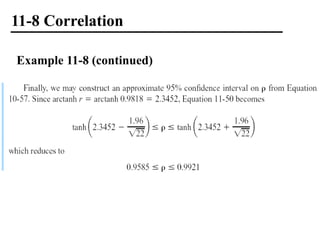
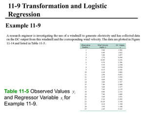
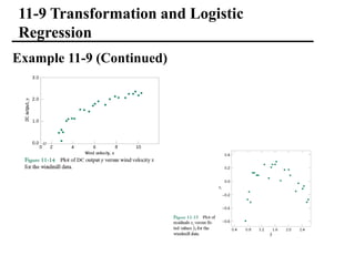
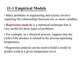
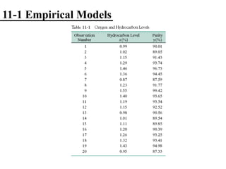
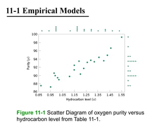
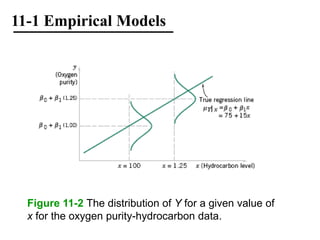
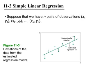
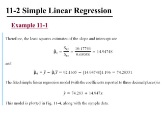
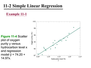
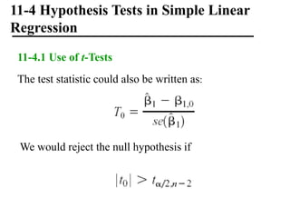
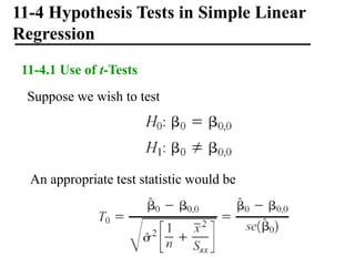
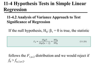
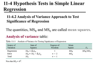
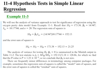
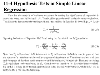
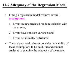
The document discusses empirical models and regression analysis as a means to explore relationships between variables, illustrated through examples like predicting chemical process yields based on temperature and analyzing oxygen purity related to hydrocarbon levels. It covers key concepts in simple linear regression, including the use of least squares to estimate parameters, hypothesis testing for significance, confidence intervals, and assumptions for model adequacy. Additionally, it introduces residual analysis, the coefficient of determination, and basic correlation concepts.

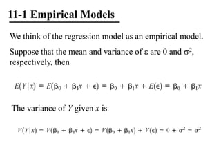
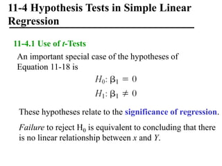
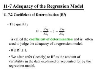
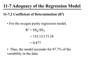
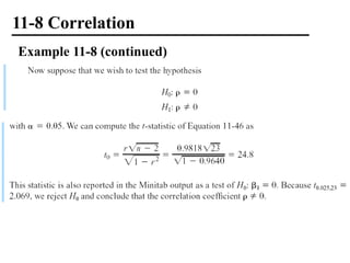
![11-7 Adequacy of the Regression Model
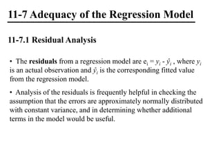
11-7.1 Residual Analysis
Figure 11-9 Patterns
for residual plots. (a)
satisfactory, (b)
funnel, (c) double
bow, (d) nonlinear.
[Adapted from
Montgomery, Peck,
and Vining (2001).]](https://image.slidesharecdn.com/advancedstatisticalmethods005-240613192439-d37b8bdb/85/Advanced_Statistical_Methods_Correlation-ppt-55-320.jpg)