This document provides a preface and table of contents for a textbook on advanced mathematical methods in science and engineering. The preface summarizes that the book covers topics like ordinary and partial differential equations, complex variables, special functions, asymptotic methods and Green's functions, with examples from fields like physics, mechanics and engineering. It is intended for advanced undergraduate and graduate students and evolved from course notes developed over many years.
![ORDINARY DIFFERENTIAL EQUATIONS 3
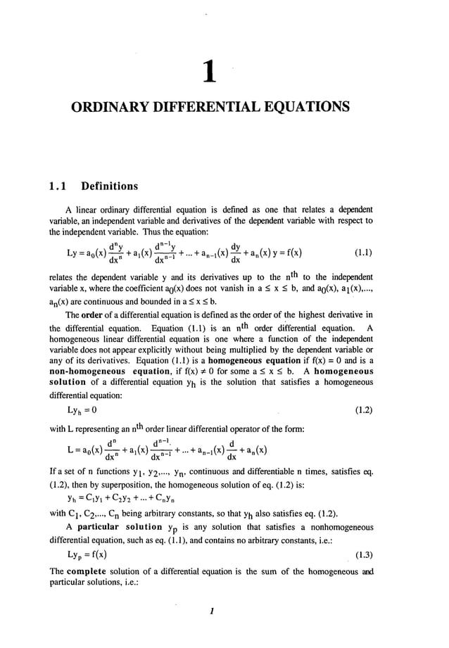
/.t(X) = exp(~¢(x)
Usingthe integrating factor, eq, (1.4) canbe rewritten in the form:
Thus,the completesolution of (1.4) can be written as:
Y=C1 exp(-~ ~(x)dx)+ exp(-~ ¢(x)dx)~ ~(x)/~(x)dx
(1.7)
(:.8)
(1.9)
1.3 Linear Independence and the Wronskian
Consider
a set of functions[yi(x)], i = 1, 2 ..... n. Aset of functionsare termed
linearly independenton(a, b) if there is no nonvanishing
set of constants 1, C
2 ..... C
n
whichsatisfies the followingequationidentically:
ClYl(X
) + C2yz(x)+ ... + CnYn(X) (1.10)
If Yl’Y2
..... Ynsatisfy (I.1), andif there exists a set of constantssuchthat (1.10)
satisfied, thenderivativesof eq. (1.10)are also satisfied, i.e.:
Cly ~ +C2Y ~ +...+CnY ~ =0
Cly ~" +C2Y~ +...+Cny ~ =0
(1.11)
-~c’ ~,(n-O_
CIY~
n-l) + C2Y(2
n-l) + ..... n-n -
For a non-zeroset of constants [Ci] of the homogeneous
algebraic eqs. (1.10) and (1.11),
the determinantof the coefficients of C
1, C
2 ..... Cn must vanish. Thedeterminant,
generallyreferred to as the Wronskian
of Yl, Y2..... Yn, becomes:
W(yl,y:~
.....
yn)=lyyin_l ) y~ ... y~n
I
(1.12)
yl°-1)... y~-’)[
If the Wronskian
of a set of functionsis not identically zero, the set of functions[Yi] is a
linearly independentset. Thenon-vanishingof the Wronskian
is a necessary and
sufficient conditionfor linear independence
of [Yi] for all x.
Example 1.2
If Yl =sin 2x, Y2= cos 2x:](https://image.slidesharecdn.com/advancedmathematicalmethodsinscienceandengineering-hayek-230318001731-2b30ece5/85/advanced-mathematical-methods-in-science-and-engineering-hayek-pdf-19-638.jpg)
![CHAPTER 1 4
sin2x cos2x 1=
W(Yt,Y2)= 2 cos 2x -2 sin 2x
I -2 ~ 0
Thus,YlandY2are linearly independent.
If theset [Yi]is linearlyindependent,
thenanother
set [zi] which
is a linear
combination
of [Yi] is definedas:
zl = °q~Yt
+/~12Y2
+ ,.. + aqnY.
z2 = ~21Yl + (~22Y2 + ..- + (X2nYn
Zn = ~nlYl + ~n2Y2 + "’" + °t~Yn
with¢xij beingconstants,is alsolinearlyindependent
provided
that:
det[otij] ~ 0, because
W(zl)=
det[otij]- W(Yi)
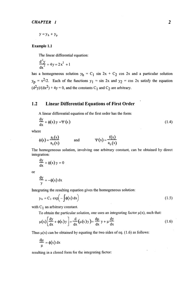
1.4 Linear Homogeneous Differential Equation of Order n
with Constant Coefficients
Differentialequations
of ordern withconstantcoefficientshaving
the form:
Ly= a0Y
(n) + aly(n-0 + ... + an_~y’
+ any= 0 (1.13)
whereao, a1 ..... an are constants,witha0 ~ 0, canbereadilysolved.
Sincefunctionsemxcan bedifferentiated many
timeswithouta change
of its
functionaldependence
onx, thenonemay
try:
y= e
mx
wheremis a constant, as a possiblesolution of the homogeneous
equation.Thus,
operating
onywiththe differentialoperator
L, results:
Ly = (aomn+ aim
n-~ +... + an_~m
+ an)e
mx (1.14)
which
is satisfied bysetting the coefficientof emxto zero. Theresultingpoly~tomial
equationof degreen:
ao
mn+ aim
n-~ + ... + a,_lm+ an = 0 (1.-15)
is called the characteristic equation.
If the polynomial
in eq. (1.15)hasn distinct roots, 1, m
2 ..... m
n, thenthere are n
solutionsof the form:
Yi= emiX,
i =1,2..... n (1.16)
eachof whichsatisfies eq. (1.13). Thegeneralsolutionof the homogeneous
equation
(1.13)canbewrittenin termsof the n independent
solutionsof (1.16):
Yh= C1emlx + C2em2x + ". + Cn
em*x (1.17)
where
C
i are arbitraryconstants.
Thedifferential operatorLof eq. (1.13)canbewrittenin anexpanded
formin terms
of thecharacteristicrootsof eq. (1.15)as follows:](https://image.slidesharecdn.com/advancedmathematicalmethodsinscienceandengineering-hayek-230318001731-2b30ece5/85/advanced-mathematical-methods-in-science-and-engineering-hayek-pdf-20-638.jpg)
![CHAPTER I 1 0
andletting:
’ (~-2)
(2~-2)’
’ @-2)
v~ y~ + v2 y + ... + v~Yn = 0
then
y(pn-1)=vlyln-1)+ v2Y(2n-1)
+ Vny(nn-1)
Thusfar (n - 1) conditionshavebeenspecified onthe functions 1, v2 ..... vn. The n
th
derivative is obtainedin the form:
y(p") : v~yln-1)+v~y(2n-1)+¯ , (,-i)
... + Vny
n -I-Vlyln)+v2Y(2
n) +... +VnY(n
n)
Substitution of the solution y andits derivatives into eq. (1.1), andgroupingtogether
derivatives of each solution, one obtains:
v~ [aoYl
~) +axyl~-O
+ ... +anY~
]+ v2 [aoY~)+
a~y(~-O
+ ... +anY
2]+...
¯ (~-1)1
+v.[aoy(n’~)+
aly(n"-l’ +... + anYn
] +aO[v~ylr’-l’+v~Y(2n-"
+ .., +vnYn
] : l:’(X)
Theterms in the square brackets whichhavethe formLyvanish since each Yi is a
solution of Ly
i =0, resulting in:
v;yl,~_,) +v~y(2n_l)
.. . +v:y(nn-1) :f(
a0(x)
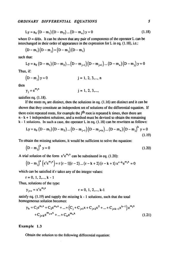
Thesystemof algebraic equations on the unknown
functions v~, v~ ..... v~ can nowbe
written as follows:
v~yi + v~Y2
Vly1 + v2Y
2
+... +vny
n = 0
+... +vny
n = 0
...... (1.25)
vyl°-2/+°-2/+...+
v:y
v~yln_,)
+ v~y(zn_l)
+... + v:y(nn_,)=
a0(x)
Thedeterminantof the coefficients of the unknown
functions [v~] is the Wronskian
of
the system, whichdoes not vanish for a set of independentsolutions [Yi]" Equationsin
(1.25) give a uniqueset of functions [v~], whichcan be integrated to give [vii, thereby
givinga particular solution yp.
Themethod
of variation of the parametersis nowapplied to a general 2nd order
differential equation.Let:
a0(x) y’+at(x) y¯+ a2(x) y = f(x)
such that the homogeneous
solution is given by:
Yh= C~Yl(X)+ C2Y2(X)
and a particular solution can be foundin the form:
yp = v~yl + vZy
2
wherethe functions v1 and v2 are solutions of the twoalgebraic equations:](https://image.slidesharecdn.com/advancedmathematicalmethodsinscienceandengineering-hayek-230318001731-2b30ece5/85/advanced-mathematical-methods-in-science-and-engineering-hayek-pdf-26-638.jpg)
![ORDINARY DIFFERENTIAL EQUATIONS 11
and
vt.y~ + v2y
2 =0
_ f(x)
v~y~ +v~y[ a0(x
)
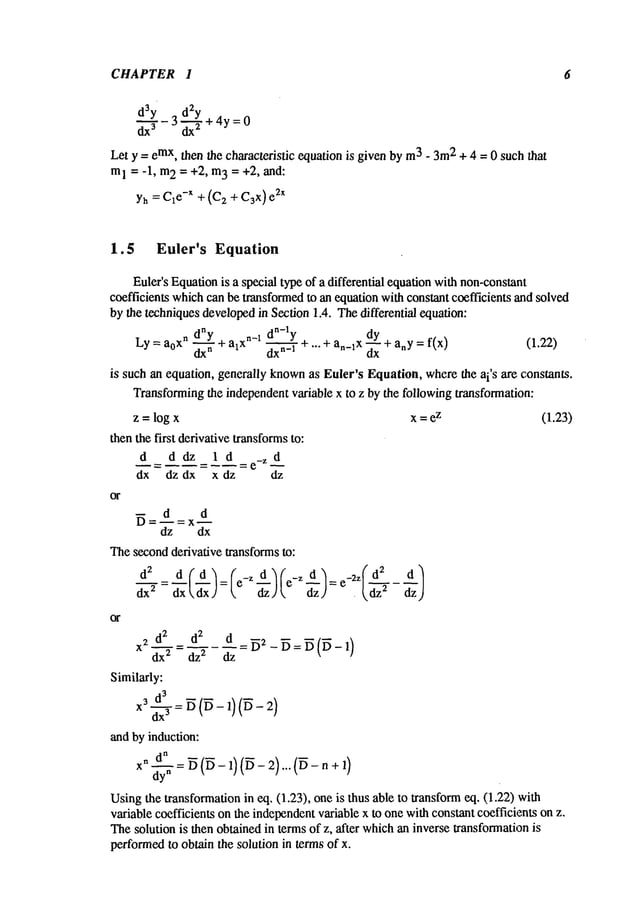
Solvingfor v~ and v2, one obtains:
. -Y2 f(x)/a0(x) y2
V|~
y~y~ - y~y~_ ao(x) W(x)
and
, y, f(x)/ao(x ) =-~ y~ f(x)
V
2
--
y~y;_ - y~y~ ao(x ) W(x)
Direct integration of these twoexpressionsgives:
and
x
v, =-I y:(r/) f(r/) dr/
ao(r/)
x
v2= +j" yl(r/) f(r/) dr/
Theunknown
functions v I and v2 are then substituted into yp to give:
X
yp =_y,(x) I yz(r/)f(r/) dr~+y_9(x) f Yl(rl)f(r])
a0(r~) W(O) J a~(~ W---~) dr/
x~y~(r/)y~_(x)-yl(x)Y2(r/)f(r/)
dr/
w(.) ,,0(7)
Example 1.7
Obtainthe completesolution to the followingequation:
y" - 4y = e
x
Thehomogeneous
solution is given by:
Yh = CIe2x + C2
e-2x
wherey~ = eZ
x, yg_= e-~-x, ao(x) = 1, and the Wronskian
is given by:
W(x)=y~y~ -y~y2 =-4
Theparticular solution is thus givenby the followingintegral:](https://image.slidesharecdn.com/advancedmathematicalmethodsinscienceandengineering-hayek-230318001731-2b30ece5/85/advanced-mathematical-methods-in-science-and-engineering-hayek-pdf-27-638.jpg)
![CHAPTER 1 12
Xe2r/ e_2x
_ e2
x e-Zn
yp = J
(-4)
!
dr/= --" e
x
3
Thecomplete solution becomes:
y = C1
e2x + C2e
-2x _ -~ e
x
1.8 Abel’s Formula for the Wronskian
TheWronskian
for a set of functions [Yi] can be evaluatedby using eq. (1.12).
However,
one can obtain the Wronskian
in a closed formwhenthe set of functions [Yi]
are solutions of an ordinarydifferential equation.Differentiating the determinantin (1.12)
is equivalent to summing
n-determinantswhereonly one rowis differentiated in each
determinanti.e.:
dW
dx
~,~.-2)
¢I
n-l)
y[
y(2
n-2)
Y~
Y~
Y:
y(n
n-2)
y(n
n-l)
Yl
+ y~’
y~n-1)
y~n-1)
Y2 ." Yn
Y~ ." Yn
Y~ "" Yn
y(n-1) y(nn-1)
y(n-l) y(nn-l)
Yl Y2 --. Yn
"" Y.
+
yl
n-2)
yl
n)
y(2n -2) ... y(~n-2)
Sincethere are twoidentical rowsin the first (n - 1) determinants,eachof these
determinantsvanish, thereby leaving only the non-vanishinglast determinant:
dW
Yl Y2 ... Yn
Yl Y[ ... Y~
In-2)
yl n) y(2 n) ...
Substitutionof (1.2) for yl
")
, i.e.:
y(n-2)
11
y!n) =- al(x...~)" (n-l) a2(x).
an-l(X)., an(x)
a0(x) Yi
- ~ Yi -
a0(x
)
...-~Yi ao(x ) Yi
(1.26)
(].27)](https://image.slidesharecdn.com/advancedmathematicalmethodsinscienceandengineering-hayek-230318001731-2b30ece5/85/advanced-mathematical-methods-in-science-and-engineering-hayek-pdf-28-638.jpg)
![ORDINARY DIFFERENTIAL EQUATIONS 13
into the determinantof (dW)/(dx),and manipulatingthe determinant, by successively
multiplyingthe first rowby an/a0, the secondrowby an_l/a0, etc., and addingthemto
the last row,one obtains:
d__~_W:
_a,(x_~)
dx a0(x)
whichcan be integrated to give a closed formformulafor the Wronsldan:
( I" a~(x)
W(x) = 0 exp~j- a --~ a x~ (1.28)
with W
0 = constant. This is knownas Abel’s Formula.
It should be noted that W(x)cannotvanish in a region < x < b unless W
0van
ishes
identically, al(x) --> ~ or ao(x) ---> 0 at some
point in a _<< b.Since thelasttwo a
re
ruled out, then W(x)cannot vanish.
Example 1.8
Considerthe differential equation of Example
1.3. TheWronskian
is given by:
W(x) = W0exp(~-3 dx) e-3x
whichis the Wronskian
of the solutions of the differential equation. Toevaluate the
constant W
0, one can determinethe dominantterm(s) of each solutions’ Taylorseries,
find the leading termof the resulting Wronskian
and then take a limit as x --> 0 in this
special case, resulting in W
0 = 9 and W(x)
= -3x.
1.9 Initial Value Problems
Fora uniquesolution of an ordinary differential equationof order n, whose
complete
solution contains n arbitrary constants, a set of n-conditionson the dependent
variable is
required. Theset of n-conditionsonthe dependent
variable is a set of the valuesthat the
dependent
variable andits first (n - 1) derivatives take at a point x = 0, w
hich can be
givenas:
y(x0) = cz0
y’(x0) =1
: a < x,x0 < b (1.29)
y(n-’)(x0) = 1
Auniquesolution for the set of constants [Ci] in the homogeneous
solution Yhcan be
obtained. Such problems are knownas Initial Value Problems. To prove
uniqueness,let there exist twosolutions YIandYlI satisfying the system(1.29) suchthat:
YI = C~y~+ C2y
2 + ,.. + CnY
n + yp
YlI = B~y~
+ B2y
2 + ... + Bny
n + yp](https://image.slidesharecdn.com/advancedmathematicalmethodsinscienceandengineering-hayek-230318001731-2b30ece5/85/advanced-mathematical-methods-in-science-and-engineering-hayek-pdf-29-638.jpg)
![CHAPTER 1 14
then, the difference of the twosolutions also satisfies the samehomogeneous
equalion:
L(yi- yn)=0
Yl (Xo)- Yi~(Xo)
= 0
(Xo)-
y (xo
)--
y~n-l)(xo)- y(n
n-l) (xo)= 0
whichresults in the following homogeneous
algebraic equations:
Aly~(Xo)+ A2y2(xo)+ ...+ A,~Y,~(Xo)
A,y~(Xo)+ A2y[(xo) +...+ Any~(Xo)
:
(1.30)
AlYln-1)(Xo)
+ Azy~n-1)(Xo)
+... + Any(~n-1)(Xo)
wherethe constants A
i are definedby:
A
i---Ci-Bi i=1,2,3 ..... n
Since the determinantof the coefficients of [A
i] is the Wronskian
of the system, which
does not vanish for the independentset [Yi], then A
i =0, and the twosolutions YIand YlI,
satisfying the system(1.29), mustbe identical.
Example 1.9
Obtain the solution of the following system:
y"+4y=0
y(O)= x _>0
y’(0) =
y = Clsin (2x) + 2 cos (2x)
y(0) = 2 =1
y’(0) = 1 = 4 C
1 = 2
suchthat:
y = 2 sin (2x) + cos (2x)](https://image.slidesharecdn.com/advancedmathematicalmethodsinscienceandengineering-hayek-230318001731-2b30ece5/85/advanced-mathematical-methods-in-science-and-engineering-hayek-pdf-30-638.jpg)
 = ix u2(x
) = e
-i x
(b) ul(x) = -x uz(x) = e
x
(c) u1(x)=l+x
2 u2(x
)=l-x
2
vl(x)
=ul- v(x) +
2 2
u~(x)andu2(x)are definedin
Section 1.4
3. Obtain the homogeneous
solution to the
(a) dzy dy 2y=0 (b)
dx z dx
d3Y-3dY+2y=0 (d)
(c)
dx
d4y
(e) ~-T- 16y= (f)
day
(g) d--~- + 16y= (h)
(i) d3--~-Y
+8a3y= (j)
dx
3
d4y ~
(k) ~-~- + 2 +a4y=O (1)
I13=sin x
followingdifferential equations:
d3y d2y 1 dy
dx
3 dx2 4 dx ÷ Y = 0
d4y
8 d2y
d-’~-- ~x~+ 16y=0
d~y
d---~ + iy =0
i = ~Z-~
dSY d4Y dd~-~Y3 2 d~y + dy
dx
5
dx4 2_.. + dx--- T ~--y=0
d3Y d2Y+ 2a3y = 0
~x
3 - a dx---
T
d~6Y+ 64y = 0](https://image.slidesharecdn.com/advancedmathematicalmethodsinscienceandengineering-hayek-230318001731-2b30ece5/85/advanced-mathematical-methods-in-science-and-engineering-hayek-pdf-31-638.jpg)
![CHAPTER 2 2 2
Letting n = m+ 3 in the first series and n = min the secondseries, so that the two
series start with the sameindex m= 0 and the powerof x is the samefor both series, one
obtains:
Co= indeterminate Cl = indeterminate c2 =: 0
Z[(m+ 2)(m+ 3)Cm+3--Cm]X m+l :0
m=0
Equatingthe coefficient of x’~’1 to zero gives the recurrenceformula:
= Cm
Cm+3(m + 2)(m + m= 0, 1, 2 ....
whichrelates Cm+
3 to cmand results in the sameconstants evaluated earlier. The
recurrence formulareducesthe amount
of algebraic manipulationsneededfor evaluating
the coefficients c
m.
Note: Henceforth,the coefficient of the powerseries cn will be replaced by an, which
are not to be confusedwith a,(x).
Example 2.2
Solvethe followingordinary differential equation aboutxo = 0:
dZy dy
X-d--~-x~
+ 3~-+xy= 0
y= an
xn
n=0
Note that ao(x) = x, al(x) =1, and a~(x) = x and %(0)= 0, whichmeansthat the equation
is singular at x = 0. Attemptinga powerseries solution by substituting into the
differential equationand combining
the three series gives:
OO
Z
~’~a x
Ly= n(n+2) anx n-l+ z~ n =0
n=0 n=0
oo
’~ a x
~+1
= 0. a0x-1 + 3a1 + n(n + 2) anxn-1 + z_, n = 0
n=2 n=0
Substituting n = m+ 2 in the first and n = min the secondseries, one obtains:
=0.ao x-1 +3al + Z[(m+2)(m+a)am+2 +am]X m+l =0
m=0
Thus,equating the coefficient of each powerof x to zero gives:
a0 = indeterminate aI = 0
as well as the recurrenceformula:
am m=0,1,2 ....
a~+2 = (m +2)(m](https://image.slidesharecdn.com/advancedmathematicalmethodsinscienceandengineering-hayek-230318001731-2b30ece5/85/advanced-mathematical-methods-in-science-and-engineering-hayek-pdf-37-638.jpg)
![CHAPTER 2 2 4
Example 2.3
Classify the behaviorof each of the followingdifferential equationsat x = 0 and at all
the singular points of each equation.
d2y . dy
(a) x d--~+ s~nX~x+ x2y =
Here, ~l(x) = slnx and ~2(X) ---- X
x
Bothcoefficients are regular at x = 0, thus x = 0 is a RP.
d2y 3
dy+x y=0
(b) Xdx----~-+
~l(x)=--3 ~2(x) =
X
Here, x = 0 is the only singular point¯ Classifying the singularity at x = 0:
Lim x(3/=3 Lim x2(1)=0
x-->O kx] x-->O
Thus x = 0 is a RSP.
(c) x2(x2 - 1 +(x-l)2 dY +
(x-l) 1
~l(X) = x2(x + 1) ~2(x) = (x - m)(x
Here, there are three singular points; x = -1, 0, and +1. Examining
each singularity:
Lim (x+l) (x-l)
x --~ -1 xZ(x+ 1)
Lim(x + 1)
2
1
x --> -1 (x - 1)(x +
xo = -1 is a RSP.
-0
Lim x (x - 1)
’ x--~0 x2(x+l)
¯ Lim x2 1
x-->O (x-1)(x+
=0
xo = 0 is an ISP](https://image.slidesharecdn.com/advancedmathematicalmethodsinscienceandengineering-hayek-230318001731-2b30ece5/85/advanced-mathematical-methods-in-science-and-engineering-hayek-pdf-39-638.jpg)
![SERIES SOLUTIONS OF ORDINARY DIFFERENTIAL EQS. 25
X_o
= +1
Lim(x-1)(T)~ -- 1!,
x--~l x ix+l)
Lim(x - 1)
2
1
x--~1 (x - 1)(x+
=0
x0 = +1 is a RSP
,2.4 Frobenius Solution
If the differential equation(2.4) has a RegularSingularPoint at 0, then o
ne or both
solution(s) maynot be obtainable by the powerseries expansion(2.3). If the equation
has a singularity at x = x0, one canperforma linear transformation(discussedin Section
2.2), z =x - 0, and seek asolution about z = 0.Forsimp
licity, a so lution vali d in t he
neighborhood
of x = 0 is presented.
For equations that havea RSPat x = x0, a solution of the form:
y(x)= E an(x- n+a (2.5)
n=0
can be used, wh’ere~ is an unknown
constant. If x0 is a RSP,then the constant ~ cannot
be a positive integer or zero for at least one solution of the homogeneous
equation. This
solution is knownas the Frobenius Solution.
Since~ l(X) and~2(x)can, at most,be singular to the order of (x-x0)-~ and(x-x0)
2,
then:
(x-x0)2
2(x/
are regular functions in the neighborhood
of x = x0. Thus,expandingthe abovefunctions
into a powerseries aboutx =x0 results in:
(X - X0) ~l(X) : ~0 + £Zl(X - X0) + ~2(X- X0)2 = E~k(X- X0)k(2.6)
k=0
and
(X--X0) 2 ~2(X)=~0 +[~I(X--X0)+~2(X--X0)2+ E[~k(X-X0)
k
k=0
Transforming
the equation by z = x - x0 and replacing z by x, one can discuss solutions
about x0 = 0. TheFrobeniussolution in eq. (2.5) and the series expansionsof al(x)
a2(x) about0 =0 ofeq.(2.6) are subs
tituted into the differential equation (2.4), such
that:
~o
[ ~O~kxk-I ~ ~(n+O’)anxn+~r-1
Ly= E(n+cr-1)(n+o’)anxn+a-2
n = 0 Lk =0 ]Ln =0](https://image.slidesharecdn.com/advancedmathematicalmethodsinscienceandengineering-hayek-230318001731-2b30ece5/85/advanced-mathematical-methods-in-science-and-engineering-hayek-pdf-40-638.jpg)
![CHAPTER 2 26
k-2 n+ff
+ kX anX =
Lk = 0 JLn= 0 J
Thesecondterm in (2.7) can be written in a Taylorseries formas follows:
where
(72.7)
Lk = 0 .JLn= 0
k=n
+((~a°(~2 +((~+ 1) ax(~l +((~+ 2) a2c~°) x2 +"’+I X((~+
k,k =0
O0
= ~ C X
n+ O’ -2
L, n
n=0
= xO-2[oo~0a0
+ (ga0oq + (~ + 1) al,x0)
X
n +...]
k=n
Cn = ~_~((r+k)a k C~n-
k
k=0
Thethird term in eq. (2.7) can be expressedin a Taylorseries formin a similar manner:
~k
xk-2 anXn+a
= Z-~
~dnxn+°’-2
Ln=O JLn=O J n=O
whem
k=n
X ak ~n-k
k=0
Eq. (2.7) then becomes:
Ly = x
°-2
(n + o" - 1)(n + o’) n + cnx n + d~x" (2.8)
Ln=0 n=0 n=0
=x(~-z{[(~((~-
1) + (~C~o
+J~o]ao +[((~(~r + 1)+o +I~o) a, + ((~oq
+[],)
+ [((o" +1)(o" +2) +((r o + Po)
az+(((r + 1)oq
+1 + (o’~x~ + f
la) ao] xz
+...+ [((n+ (~- 1)(n+ (~) + ((~+ o +l~o) a~ +((( ~+
n-1)al+ I~) a
+(((r + n- 2)ctz + j~) a._z +... +(((r + 1) o~._~+/~._~) al +((ran + j~.)
Definingthe quantifies:
f(cr) =(r(o" - 1) +o + flo](https://image.slidesharecdn.com/advancedmathematicalmethodsinscienceandengineering-hayek-230318001731-2b30ece5/85/advanced-mathematical-methods-in-science-and-engineering-hayek-pdf-41-638.jpg)
![SERIES SOLUTIONS OF ORDINARY DIFFERENTIAL EQS. 27
then eq. (2.8) can be rewritten in a condensed
form:
Ly: x
°-2 {f(ff)a0 +[f(ff + 1)aI + fl(ff)ao] x +[f(ff + 2)a2+ fl(6 +
+f2 (ff)ao2 +.. . + [f(ff + n)n + fl(ff + n- 1)an
1 + ...+fn (ff)]xn + ...}
=x°-2 f(~r) 0+ ~f( ff+n) a n+
(~+n-k) an_ k x
~ (2.9)
n=lL
Eachof the cons~ts a~, a~ ..... ~ .... c~ ~ written ~ te~s of %, by equating the
c~fficien~of x, x
~ .... to zero as follows:
a~(a) : f~(a)
f(a+1)
a2(a) = f~(a + 1) a~ + f2(a)
-fl(ff) f(ff+l) + f2(ff) f(ff+l)at g2(ff)
= f(6 + 1) f(6 + f(’~ ~) a°
a3(6) f~(6 + 2)a2 + f2(6 + 1) al + f3(
.... -":: .... f(6 +3) ~
and by induction:
gn
(6)
n > 1
a n (6) = - ~ -
= f(6+3) a0
(2.10)
Substitutionof an(o
) n = 1, 2, 3 .... in termsof the coefficient ao into eq. (2.9) results
the followingexpressionfor the differential equation:
Ly = xa-2f(o") a
o (2.11)
and consequentlythe series solution can be written in terms of an(a), whichis a function
of 6 and a0:
y(x,6) = x° + Ean(6) Xn +O (2.12)
n=l
Fora non-trivial solution; ao ¢ 0~eq. (2.7) is satisfied if:
f(o-) = a(o- - 1) o"+/3
0 = 0 (2.13)
Eq. (2.13) is called the Characteristic Equation, whichhas two roots I and . o
2.
Depending
on the relationship of the tworoots, there are three different cases.
Case(a): Tworoots are distinct anddo not differ by an integer.
If 61 ¢ 02 and61 - 02 ¢ integer, then there exists twosolutions to eq. (2.7) of the form:](https://image.slidesharecdn.com/advancedmathematicalmethodsinscienceandengineering-hayek-230318001731-2b30ece5/85/advanced-mathematical-methods-in-science-and-engineering-hayek-pdf-42-638.jpg)
![CHAPTER 2 2 8
yl(x) = 2an(or,) xn+~rl
n=0
and (2.14)
y2(x) = ~a.(~r2)
n=0
Example 2.4
Obtainthe solutions of the followingdifferential equationabout x0 = O:
Since x = 0 is a RSP,use a Frobenius solution about x0 = 0:
y = ~an
xn+~r
n=0
such that when
substituted into the differential equationresults in:
~ [(n+~)~-~]an xn+~’:2+ 2anxn+°=O
n=0 n=0
Extractingthe first two-lowestpowered
termsof the first series, such that each of the
remainingseries starts with x~ one obtains:
+ (n+~)2_~ ~"a x
anxn+~-2
+’9
"~ L,n =0
n=0
Changingthe indices n to m+ 2 inthe first series and to min the secondand combining
the tworesulting series:
m=0
Equatingthe coefficients of x~-l and xm+~
to zero and assumingao ~ 0, there results
the followingrecurrence formulae:
am m=0, 1,2 ....
a~÷~=(m+~+:z)2_
N
andthe characteristic equation:](https://image.slidesharecdn.com/advancedmathematicalmethodsinscienceandengineering-hayek-230318001731-2b30ece5/85/advanced-mathematical-methods-in-science-and-engineering-hayek-pdf-43-638.jpg)
![CHAPTER 2 30
The final solution y(x), setting 0 =
1 ineach series gives:
Y(X)=clyl(x)+c2Y2(X)
Case(b): Twoidentical roots O-1=¢r2 = O-~
If ~l = or2 = Cro, then only one possible solution can be obtained by the methodof
Case(a), eq. (2.14), i.e.:
yl(x) = E an(o-o) xn+~r°
n=O
wherea0 =1.
Toobtain the secondsolution, one mustutilize’eqs. (2.11) and(2.12). If ~1 = ~r2
co, then the characteristic equationhas the form:
f(o-) : (o-- O-o)
2
and eq. (2.11) becomes:
Ly(x,o-) = xa-2(o- - O-o)2ao (Z.15)
wherey(x,o) is givenin eq. (2.12). First differentiate eq. (2.15) partially with
~Ly= L °aY(X’o-) : ao[2(a - ao) + (a- ao)2 logx] ~r-2
where
~d xa=x
alo gx
If O-= O-o,then:
--o
L 00- do-=o-0
Thus,
the
second
solution
satisfying
the
homogeneous
differential
equation
isgiven
by:
y(x)
Usingthe form of the Frobenius solution:
y(x,o-)= xa + Ean(°’) xn +a
n=l
then differentiating the expressionfor y(x,~) withff results in:
ay(x,cr)a
oo
=a0x~ log x + Ea~(~) n÷~ +an(o ) xn+~ lo gx
n=l n=l](https://image.slidesharecdn.com/advancedmathematicalmethodsinscienceandengineering-hayek-230318001731-2b30ece5/85/advanced-mathematical-methods-in-science-and-engineering-hayek-pdf-45-638.jpg)
![SERIES SOLUTIONS OF ORDINARY DIFFERENTIAL EQS. 31
--logx Xan(o) xn÷°
n=O n=l
Thus,the secondsolution for the case of equal roots takes the formwith a0 = 1:
yz(x) = logx Xan(O0)xn+’~°
n=O n=l
= yl(x)logx+ ~" a’ to ~ x
n+°°
Z_, n~, o/
n=|
(2.16)
am+1 =
where
Example 2.5
Solvethe followingaifferential equation about x
o = 0:
2dZY 3xdY+(4_x)y=0
x dx-- ~- dx
Since xo = 0 is a RSP,then assumea Frobeniusseries solution which, whensubstituted
into this differential equationresults in:
X(n + ~_ 2)2 a.x’+a-2 ~ax
- z~n =0
n=0 n=0
or, uponremoving
the first term and substituting n = m+ 1 in the first series and n = m
in the secondseries results in the followingequation:
~o-2/z
a0x
°-z
+~[~m
+o-
1)
2am+, -am
.]x
m+°-~ --0
m=0
Equatingthe coefficient of x
~2 to zero, oneobtains withao # 0:
(o"- 2)2 = 0 or cr~ = a2 = 2 = ao
Equatingthe coefficient of xm÷ox
to zero, one obtains the recurrence formulain the form:
am
m=0,1,2 ....
(m
+~r-1)
2
and by induction:
a.(a)
ao
_ al ao
(a- I)2o’2(o
. +1)2...(o
. +n- 2)
2
Thus,the first solution correspondingto o = o0 becomes:
n=l,2 ....](https://image.slidesharecdn.com/advancedmathematicalmethodsinscienceandengineering-hayek-230318001731-2b30ece5/85/advanced-mathematical-methods-in-science-and-engineering-hayek-pdf-46-638.jpg)
![SERIES SOLUTIONS OF ORDINARY DIFFERENTIAL EQS. 33
If gk(ff2) vanishes, then ak(~z)is indeterminateandone maystart a newinfinite
series withak, i.e.:
k-lor~ an(a2) xn+~r2 +ak
Y2(X) : a0
n=0 ~ / n=k~" ak
k-1 or ~,
=a 0 y, [an(~2)] n÷~2 ÷ ak m~ (.am~2)) xm+~ (2.1"/)
n----0 =0
It can be shown
that the solution precededbythe constant ak is identical to Yl(X),thus
one can set ak = 0 and ao = 1. Thefirst part of the solution withao maybe a finite
polynomialor an infinite series, dependingon the order of the recurrenceformulaand on
the integer k.
If gk(O2)does not vanish, then one mustfind another methodto obtain the second
solution. Anewsolution similar to Case (b) is developednext by removingthe constant
o - o~ fromthe demoninator
of an(o). Sincethe characteristic equationin eq. (2.11)
given by:
Ly(x,0.) = a0xa-2f(0.) = aoxa-Z(~r - 0.~)(0. - ¢rz)
then multiplyingeq. (2.18) by (o - 02) and differentiating partially witho, oneobtains:
-~ [(0.-0.2)Ly]= ~-~ [L(0.- 0.~) y(x,0.)] = L[-~(0.- 0.:~)
= ao x~’-2 0. - 0.1 0. - 0"2
Thus,the function that satisfies the homogenous
differential equation:
0" =0"2
gives an expressionfor the secondsolution, i.e.:
y~(x)
=--~
(0.-0.~)y(x,0")[
a =0.2
(2A9)
TheFrobeniussolution can be divided into twoparts:
n=k-1
y(x,0.)= ~a.(alx"+~r= ~a.(0.lx"+a+ ~a.(0")x
n=0 n=0 n=k
so that the coefficient ak is the first termof the secondseries. Differentiating the
expressionas given in eq. (2.19) one obtains:](https://image.slidesharecdn.com/advancedmathematicalmethodsinscienceandengineering-hayek-230318001731-2b30ece5/85/advanced-mathematical-methods-in-science-and-engineering-hayek-pdf-48-638.jpg)
![CHAPTER 2 34
~--~[(~- if2) Y(X,~)]
n=k-1 n=k-1
=logx, E(ff-ff2)an(ff)xn+ff+ ~(ff-ff2)a~(ff)x
n+ff+
n=0 n=0
+ 2[(~-~2)a~(ff)l ~+~ +logx
n=k n=k
It shouldbe no~d~t ~(ff) = - (gn(ff))/(ffff+n)) does not con~n~e te~ (if’if2)
denominatoruntil n = k, ~us:
~d for n=0, 1,2 ..... k-1
(~- ~2)a~ (")[~ =
~er¢fore, ~ s~ond solution ~ ~e fo~:
n=k-1
y2(x)= (~- ~2) y(x,~)~ = ~2 2a~(~2)x
n=O
X [( ] x ~+~’ +logx ~-ff~)a~(~ x
~+~’
+
n=k n=k
(2.20)
It c~ ~ shown~at ~e l~t infinite ~fies is pro~onal my~(x).
E(o-~2)anCo)xn+° + E(c~-c)2)an(O)X
n+O
n=O n=k
n=k--1
E an(~) xn+°
n=0
Example 2.6
Obtainthe solutions of the followingdifferential equationabout x0 = O:
2
9
Since xo -- 0 is a RSP,then substituting the Frobeniussolution into the differential
equationresults in:
- ~’ a X
n+ff
n+ff)2 an xn+°-2+ ~_~ n =0
= n=0
which, uponextracting the two terms with the lowest powersof x, gives:](https://image.slidesharecdn.com/advancedmathematicalmethodsinscienceandengineering-hayek-230318001731-2b30ece5/85/advanced-mathematical-methods-in-science-and-engineering-hayek-pdf-49-638.jpg)
![SERIES SOLUTIONS OF ORDINARY DIFFERENTIAL EQS. 35
(~r
2 --~] a0
x°-2 +[(o+1)
2 --~] alx°-I +
m=0
Thus,equatingthe coefficient of each powerof x to zero; one obtains:
and the recurrence formula:
a
m am
a,=*2= (m+2+tr)=_9~ = (m+a+~)(m+a+7//2)
Solvingfor the roots of the characteristic equationgives:
3 3
ax =2 ~2 =-’~ al - 02=3 = k
Usingthe recurrenceformulato evaluate higher orderedcoefficients, one obtains:
a0
m=0,1,2 ....
al
a3=
(o-+ 3/2Xo.+9/2
)
a2 ao
a,~=(0. +5/Z2XO.
+ ;~) = (0. +~,~)(0. +5~2){0.+7~2X0.
a3 al
Thus,the oddand evencoefficients a,, canbe written in termsof ao andaI by inductionas
follows:
ao
a2,~ =(-1)’~ (or +l~)(cr + 5~)... (¢r + 2m-3~). (tr + 7~)(o- +1~/~1... (o-
a2m+l ’ ’ ’3 7
al
for
Toobtain the first solution corresponding
to the larger root ~1= 3/2:
ao = indeterminate ¯
m=1,2,3 ....](https://image.slidesharecdn.com/advancedmathematicalmethodsinscienceandengineering-hayek-230318001731-2b30ece5/85/advanced-mathematical-methods-in-science-and-engineering-hayek-pdf-50-638.jpg)
![CHAPTER 2 3 6
a1 =a3 =a5 =...=0
a2m(3/2) = (_l)m 3ao(2m+ 2)
(2m+ 3)!
and by setting 6ao = 1:
m=1,2,3 ....
y~(x)=g z_,, ,
(2m+3)! ~( -1)m(m+
m= 1 m= 0
(2m+ 3)
Toobtain the solution co~esponding
to the smaller root:
3
ff2 = -- ~, whe~ ff~ - ~ = 3 = k
a0 = indete~nate
a1 =0
a2m(_3/2) = (_l)m (-a0)(2m-
Thecoefficient ak = a3 mustbe calculated to decide whetherto use ~e secondfo~ of the ~
solution (2.20). Using the recu~encefo~ula for ~ = -3/2 gives:
0
a3 0 (indete~nate)
Sothat the coefficient a3 is not unbounded
and can be used to st~ a newseries:
(-1) m+la3 " )l]
a~m+~= (~+~)...(o+2m-~).(ff+.l~)...(~+2~+~
(1)
~*~ 6a3m
= - ,m=2, 3,4 ....
Thus,the secondsolution is obtained in the form:
(2m- 1) x2m-3/2
m= 1
(2m) + a3x3/2
~
m X
2m-1/2
+6a
(2m+
l
m=2 "
m=0---- . 6%m=0~(-1)~ (2m+3)~
Notethat the solution sta~ing with ak = a3 is Yl(X), whichis extraneous. Letting ao=
and a3 = 0, the secondsolution becomes:](https://image.slidesharecdn.com/advancedmathematicalmethodsinscienceandengineering-hayek-230318001731-2b30ece5/85/advanced-mathematical-methods-in-science-and-engineering-hayek-pdf-51-638.jpg)
![CHAPTER 2 38 .
where
6a
o wasset equalto 1.
Thesolutioncorresponding
to the smallerroot 02= -1 canbeobtainedafter checking
a3(-1):
a3(-1) oo
Using
the expression
for the second
solutionin (2.20)oneobtains:
n=2 oo ,
YzCX)=EahC-l) xn-l+ E[(~+l)a~(~)]
x=-x
n=O n=3
+ logx E[(O+ 1) an(O)]Oxn-1
n=3
Substitutingfor an(o
) andperforming
differentiationwithoresults in:
(~r+1) an(~r) a°
(o- 1)~r(cr+2)... (or+n- 2)(~r
+2)(~r
+3)... (o"
a0 = a0
(o"+ 1) n(o’)lcr =
-1= (-2)(-1) 1.2..... (n - 3) 1.2.3..... n 2 (n
{( 1) ()}’ -a°
.~__~__I+i+~l + 1 1
Lo-1 o 0+2 ""+--+--
o+n-2 0+2
[(0+1) an (0) =
o=-1 -2-- 1.1.2.....(n- 3) 1.2.....
[_~ 1 1 ~ ~]
" - -1+1+--+’"+’~-3 +1+2 +’"+
_ a0 [-~+ g(n- 3)+ g(n)]
2(n- 3)
where
g(n) = 1 + 1/2 + 1/3 +...+ 1/n andg(0)
Thesecondsolutioncanthus bewrittenin the form:
Y2(X) = 1 1 + x 1 E° ° xn-I r 3
--’~ ~’--’~ (n--_~!n!L-’~+g(n-3)+g(n)
n=3
oo
xn_l
+½logXn~=
3n, (--h-S-_
3)
t
which,
uponshiftingtheindicesin theinfinite series gives:
(o - 1) 0(0+ 2)... (o +n - 2)(0+2)(0+ 3) ... (0
1 1
+~+...+ -
0+3 o+n+l
n=3,4,5 ....](https://image.slidesharecdn.com/advancedmathematicalmethodsinscienceandengineering-hayek-230318001731-2b30ece5/85/advanced-mathematical-methods-in-science-and-engineering-hayek-pdf-53-638.jpg)
![SERIES SOLUTIONS OF ORDINARY DIFFERENTIAL EQS. 39
Y2(X)=X-I 1X____+ ....
1 ~_~
xn+2[ __3
2
]
2 4 2 n! (n + 3) ! + g(n)+ g(n
n=O
n=0(n+3)
!n!
Thefirst series can be shown
to be 3Y1(X)/4
whichcan be deleted fromthe second
solution, resulting in a final formfor Y2(X)
as:
y2(x)=x_l__+___l x 1 xn+2
2 4 2 n!(n+3)![g(n)+g(n+3)]+ log(x)yl(x)
n=0](https://image.slidesharecdn.com/advancedmathematicalmethodsinscienceandengineering-hayek-230318001731-2b30ece5/85/advanced-mathematical-methods-in-science-and-engineering-hayek-pdf-54-638.jpg)
![SERIES SOLUTIONS OF ORDINARY DIFFERENTIAL EQS. 41
Obtainthe general solution to the followingdifferential equationsabout x = Xoas
indicated:
(a)
d--~--
(x-d2y
1)d~Yux
+y =0 aboutXo=: 1
d2y
Co) d--~--(x-1)2y=O aboutxo= 1
(c) x(x "d2y 6(x 1)d-~-Y+6y=O aboutxo 1
-2 Grx + -.x =
(d) x(x + 2) ~-~2Y+8(x + 1)--~+ about xo=-1
Section 2.3
4. Classifyall the finite singularities, if any, of the followingdifferential equations:
(a) 2 d2y dy
d--~- + X~x+(x:Z-4) y = (b)
(c) (1- x21 d~ --2x dY +6y (d’)
x ~ dx" dx
¯ d2y dy
(e) s~nx d-~+coSX~xx+y = (f)
(g) (x- 1)z d2~Y+ (x2-1) dY+ x2y
dx ~ ~ ~ dx
Oa)
x2 d~Y+(l+x) dY +y =
dx" dx
2
x
2~ d~Y
- 2x d-~-Y+(1+ x)Zy=
x(1-
! dx
2 (Ix
d2y dy
xz tan x~-+ x~ + 3y =0
Section 2.4
Obtainthe solution of the followingdifferential equations, valid in the neighborhood
of x =O:
(a) x2(x + 2)y" + x(x- 3) y’+ 3y
d~2
y 2x~] dY-3y= 0
CO) 2X
2
+ [3x + idx
@
(c) x
2
+[x+ Jdx L 4 2J
y= O](https://image.slidesharecdn.com/advancedmathematicalmethodsinscienceandengineering-hayek-230318001731-2b30ece5/85/advanced-mathematical-methods-in-science-and-engineering-hayek-pdf-56-638.jpg)
![3
SPECIAL FUNCTIONS
3.1 Bessel Functions
Besselfunctions
are solutionsto the second
orderdifferentialequation:
x2 d’~"2+xdy+(xz-pz)y=Odx
’ (3.1)
where
x = 0 is a regularsingularpointandpis a real constant.
Substituting
a Frobenius
solutioninto the differentialequation
results in theseries:
+ E{[(m +2 + 6)2 - p2]am+2+ am}Xm+°
:
m=0
Fora0 v 0, 62- p2= 0, 6t = p, 62= -p and6t - 62= 2p:
[(0"+1)a-p:~]a~=
a
m
am+z= (m +2+o._ pXm+2+o.+ ) m=O,1,2 .... (3.2)
Thesolutioncorresponding
to the larger root 61 = p canbeobtainedfirst. Excluding
thecaseof p= -1/2, then:
a1= a3 =a5= ... 0
a
m
am+2 = (m+2)(m+2+2p) m=0, 1, 2....
ao
a2 = 2Zl!(p+l)
a2 a0
a,~= 4(4+2p)=242!(p+l)(p+2)
ao
a6 = 263!(p+lXp+2)(p+3)
43](https://image.slidesharecdn.com/advancedmathematicalmethodsinscienceandengineering-hayek-230318001731-2b30ece5/85/advanced-mathematical-methods-in-science-and-engineering-hayek-pdf-58-638.jpg)
![CHAPTER 3 44
and, by induction:
a
o
a2m = (-1)m 22mm!(p + 1)(p + 2)... (p
Thus, the solution correspondingto ~1 = P becomes:
oo
x2m+
p
Yl(x) ~Z_~
(-1)m2amm!
(p + 1)(p + 2)... (p
a0
xp + a0
m=l
Usingthe definition of the Gamma
function in Appendix
B. 1, then one can rewrite the
expression
for y I(X) as:
Yl(X):ao xp+a
0 E(-1)
m
m=l
r(p +1) X
2m+p
22m m! F(p + m+ 1)
= a0F(P + 1)2 p ] (x~2)p ¢¢ (x~2)2m+p
F(---~"~ + E (-1)mm!F(p+m+l)
[ m--1
Definethe bracketedseries as:
Jp(x)= ~ (-1)~m~F(p+m+l) (3.3)
m=0
wherea0 F(p+l) 2Pwasset equal to 1 in Yl(X). Thesolution Jp(x) in eq. (3.3)
as the Bessel fu~efi~ ~f ~he first ~ ~f ~rder p.
Thesolution co~esponding
to the smaller root ~2 = -P can be obtained by
substituting -p for +pin eq. (3.3) resulting in:
~
(X]2)2m-p
(3.4)
y2(x)=J-p(x) = ~ (-1)~m~F(_p+m+l)
m=0
J_p(x) is known as the Bessel f~eti~ ~f t~e seeing ~nd ~f ~rder
If p e integer, then:
y~ = c~Jp(x) + c~J_p(x)
Theexpression for the Wronskian
can be obtained from the fo~ given in eq. (1.28):
W(x) = 0 ex - = W0
e -l°gx = w0
x
W(Jp(X),J_p(X)) = Jp(X)J’_.p(x) - J~(x) wO
x
Thus:
Lim x W(x) -~ o
x---)](https://image.slidesharecdn.com/advancedmathematicalmethodsinscienceandengineering-hayek-230318001731-2b30ece5/85/advanced-mathematical-methods-in-science-and-engineering-hayek-pdf-59-638.jpg)
![SPECIAL FUNCTIONS 45
Tocalculate W
0, it is necessaryto accountfor the leading termsonly, since the formof
W- 1/x. Thus:
p/:
JP r(p+l) J[ r(p+l)
J-P r0- P) J’P r(1- p)
-2p = 2
Lim x W(Jp,J_p) = Wo= F(p+ 1) F(I_
r(p)r(1-p)
x.->o
Since:
r(p) r(1- p) = ~r (AppendixB1)
sin
then, the Wronskian
is given,by:
-2 sin p~
W(Jp,J_p) = (3.5)
Anothersolution that also satisfies (3.1), first introducedby Weber,takes the form:
cosp~ Jp(x) - J_p(x)
p ~ integer
Yp(x)
sin p~r
such that the general solution can be written in the form known
as Weberfunction:
y = Cl Jp(x) + 2 Y
p(x) p ~ integer
Usingthe linear transformation formula, the Wronskian
becomes:
W(Jp,Yp)= det[aij] W(Jp, J-p)
as given by eq. (1.13), where:
t~ll =1 0[12 = 0
a22= - 1/sin det[aij ] ="1/sin p~
0~21 = COt pzr
so that:
(3.6)
( ) , ,__2 (3.7)
WJp,Yp = JpYp - JpYp = ~x
whichis independentof p. ~,
3.2 Bessei Function of Order Zero
If p =0 then ~l = (52 = 0 (repeated roo0, whichresults in a solution of the form:
m= 0 (m!)2](https://image.slidesharecdn.com/advancedmathematicalmethodsinscienceandengineering-hayek-230318001731-2b30ece5/85/advanced-mathematical-methods-in-science-and-engineering-hayek-pdf-60-638.jpg)
![CHAPTER 3 4 6
Toobtainthe second
solution, the methods
developed
in Section(2.4) axeapplied.
From
the recurrence
formula,eq. (3.2), oneobtainsthe following
bysetting p =
am
am+2 = m=0, 1, 2....
(m
+a+2)
z
Again,byinduction,onecanshow
that the evenindexed
coefficientsare:
a2m= (-1)
m at m=1,2....
(0-+ 2)z(0-+2.. . (0- + 2m
z
y(x,0-)
atxa + atZ(-1)m
m=l
x2m+a
(0-+ 2)2(0
. +4)~ ... (0-+ 2m)
2
Using
the formfor the second
solutiongivenin eq. (2.16), oneobtains:
y2(x)=°~Y(X’0-) = atxa logx +ao logx ~ (-1)mx2m+a
c90- 0-0 = 0
m
=1 (0-+2)2(a--’-~"~-~
+2m)z
-2a0 E(-I) m (0- + 2)2(0. + z "" (0. + 2m
)2 ,0 . +~ +~ +. .. +~
m=l
0.+4 o’+2m 0.=0
which
results in the second
solutionY2as:
oo
y2(x) = logx Jo(x)+ E(--1)m+l [~’2)2rn
g(m)
Ixl~
m= 0 (m!)~
Define:
Vo(X) (r-log2)J0(x)]
m= 0 (m!)2
wherethe EulerConstant7 = Lim
(g(n) - logn) = 0.5772......
SinceYo(x)
is a linear combination
of Jo(x)andY2(X),
it is also a solutionof the
(3.1) as wasdiscussedin Sec. (1.1). Yo(x)is known
as the Besselfunction
second kind of order zero or the Neumann
function of order zero.
Thus,the complete
solution of the homogeneous
equationis:
Yh= cl J0(x) + c2 Y0(x) if p =0
(3.9)](https://image.slidesharecdn.com/advancedmathematicalmethodsinscienceandengineering-hayek-230318001731-2b30ece5/85/advanced-mathematical-methods-in-science-and-engineering-hayek-pdf-61-638.jpg)
![SPECIAL FUNCTIONS 4 7
3.3 Bessel Function of an Integer Order n
If p = n = integer ~ 0 then ~1 " ~2 = 2n is an eveninteger. ThesoIution
correspondingto ~l = + n can be obtained from(3.3) by substituting p = n, resulting in:
E(-1)(½12m÷o (3.10)
m!(m+ n)!
m=0
Toobtain the secondsolution for ~2= -n, it is necessaryto checka2n(-n
) for
boundedness.Substituting p = n in the recurrence formula(3.2) gives:
am m=0,1,2 ....
am+2=(m +2+o’- n)(m+2+o’+n)
a1 = a3 ..... 0
so that the evenindexedcoefficients are givenby:
(-1) ma
0 m=1,2,3 ....
a2m= (~ + 2- n)... (~ + 2m-n). (~ + 2 + n)... (~ + 2m
It is seen that the coefficient a2n(~= -n) becomes
unbounded,
so that the methods
solution outlined in Section (2.4) mustnowbe followed.
oo
x2m+
o.
y(x,~r) a0
xa ~"’~zLA-1)m
(or + 2 - n)... (~r +2m- n). ((r +2 +n)... (~r
+ a0
m=l
Then,the secondsolution for the case of an integer differencek = 2nis:
y2(x) : ~-{(~r-if2)y(x, ff)}o=a2 = ~{(ff + n)y(x,~)},___
n
Usingthe formulafor Y2(X)
in eq. (2.20), an expressionfor Y2results:
m=~ ~n- 1
x2m_
n
y2(x) zLA-1)m
(2- 2n)(4- 2n)... (2m- 2n). 2.4-...
a0
m=0
+ a0
’(o + 2 - n) ... (o + 2m- n): ~-’+"~+n) ... (o +2m
:n ~=-n
r m
]
n)
+ ao logx ~ ! x
2m-n
m~__n
L (~ + 2- n)...(~ + 2m-n)-(a + 2 + n)...(~ +
---- ~ ---- -n
Thus, the solution correspondingto the secondroot ~ = -n becomes:](https://image.slidesharecdn.com/advancedmathematicalmethodsinscienceandengineering-hayek-230318001731-2b30ece5/85/advanced-mathematical-methods-in-science-and-engineering-hayek-pdf-62-638.jpg)
![CHAPTER 3 48
Y2(X) = -’~
m=O
(n - m- 1)! +log x Jn(x)+ ~ g(n- 1)
] oo (X/2)2m+n [g(m)+ g(m +
-~" ~ (-1)m m! (m +
m=0
ao 2
-n+l
where - wasset equal to one.
(n
Thesecondsolution includes the first solution given in eq. (3.10) multiplied by1/2
g(n - 1), whichis a superfluouspart of the secondsolution, thus, removing
this
component
results in an expressionfor the secondsolution:
m-~.~- (x~ (n- m,1),
y2(x)=logxJn(x)_l.~ -n
"--’ m!
m=0
__.1 ~ (_l)m (x//2)2m+" [g(m)+g(m+n)]
2 m! (m + n)!
m=0
Define:
Yn(x) = ~[(~’- log2)JnCx) Y2
Cx)]
~f
[
m= n-1 (x~)2m-"
= ~’ + log(~)] J,~(x)--~
m=O
(n - m- 1)
_1 ~(_l)m (~)2m+. [g(m)+g(m+n)]
(3.11)
2 m!(m+n)!
m=0
where Yn(X) is knownas the Bessei function of the second kind of order n,
the Neumann
funetlon of order n. Thus. the solutions for p = n is:
Yh= ClJn(x) + C2Yn(x) if p =n =integer
Thesolutions of eq. (3.1) are also knownas Cylindrical Bessel functions.
Thesecond solution Yn(x) as given by Neumann
corresponds to that given by Weber
for non-integerordersdefinedin (3.6). Sincesin prr -~ 0 as p --> n =integer, cos (tin)
(-1)n as p -~ n, and:
J_n(x) = (-1)nJn(x)
then the form(3.6) results in an indeterminatefunction. Thus:
Y,(x)= Lim c°sPnJl’(x)-J-l’(x)
p -~ n sin pn](https://image.slidesharecdn.com/advancedmathematicalmethodsinscienceandengineering-hayek-230318001731-2b30ece5/85/advanced-mathematical-methods-in-science-and-engineering-hayek-pdf-63-638.jpg)
![SPECIAL FUNCTIONS 49
=-~Zsin P~JP (x) +cos P/t ~/¢9pJP(X)-/~/cgPJ-P
ffcospTr !
= ;{~ Jp(x)-(-1)~ J_p(X)}p n (3.12)
It can be shown~at ~is ~lufion is M~a ~lufion to eq. (3.1). It c~ ~ shown~m
expression in (3. ]2) gives ~e =meexpression given by ¢q. (3.11). ~e fo~ given
We~ris most u~ful in ob~ing ~ expression for ~e Wronski~, which is idenfi~l to
the expressiongiven in (3.7).
3.4 Recurrence Relations for Bessel Functions
Recurrencerelations betweenBessel functions of various orders are of importance
becauseof their use in numericalcomputationsof high orderedBessel functions.
Starting withthe definition of Jp(x) in eq. (3.3), then differentiating the expression
givenin (3.3) one obtains:
1 E (_l)m [2(m + P)- P] (x~)2m+~’-’
J~’(x) = ~’m0 m!F(m+p+l)
(x~)2m+p-l(m+P) P E (-1)m
+1)
~ (--1)m m!F(m+p+l)
2 m!F(p+m
m=0 m=0
Using F (m + p + 1) = (m + p) F (m+ p), (AppendixB1)
J(x)=Jp_:(x)-
Jp(x)
Anotherformof eq. (3:13) can be obtained, again starting with J~,(x):
J;(x): ~ (-1)
TM
E (-m)m
(m-l)! I’(m +p+l) m!F(p+m+l)
m=0 m=0
Since (m- 1)! ~ oo for m= 0. Then:
00
(X//2)2m+p-1 +~ Jp(x)
J~(x)= (- 1)m(m_l)!F(m+p+l)
m=l
(-1)
m÷1
m=O
m!F(m+ p + 2)
J~(x)=Jp+l(X)+~Jp(x)
(3.13)
(3.14)](https://image.slidesharecdn.com/advancedmathematicalmethodsinscienceandengineering-hayek-230318001731-2b30ece5/85/advanced-mathematical-methods-in-science-and-engineering-hayek-pdf-64-638.jpg)
![CHAPTER 3 5 0
Combining
eqs. (3.13) and(3.14), one obtains another expressionfor the derivative:
J;(x) = ~[Jp_l(X)- Jp+l(x)] (3.15)
Equating(3.13) to (3.14) one obtains a recurrence formulafor Bessel functions of order
(p +1) in termsof orders p and p -
Jp+l(X ) = 2p Jp(X)- Jp_l(X) (3.16)
x
Multiplyingeq. (3.14) by xP, and rearranging the resulting expression, one obtains:
1 d
x dx [x-p Jp(x)] : -(p+~) Jp+l(x)
(3.17)
If p is substituted byp + 1 in the formgivenin (3.17) this results in:
1 d [x_(P+l) Jp+l]=x-(P+2 ) Jp+2
x dx
then uponsubstitution of eq. (3.17) one obtains:
(--1)2(~X/2[ X-p Jp] = X-(p+2) Jp+2
Thus,by induction, one obtains a recurrence formulafor Bessel Functions:
~.X dx.J [X-p Jp] = x-(P+r)Jp+r
r > 0 (3.18)
Substitution ofp by -p in eq. (3.18) results in another recurrenceformula:
(-1) xpJ_p
; x
p-rJ-(p+r/ r_>
0 (3.19)
Substitution of p by -p in eq. (3.13) one obtains:
J" X
-1 (3.20)
-p - P J-p = J-(p+l)
Multiplyingeq. (3.20) by xP, one obtains a newrecurrence formula:
1 d
X dx [X-p J_p(X)] = -(p+I) J_(p+l)(X)
(3.21)
Substitution of p +1 for p in eq. (3.20) results in the followingequation:
xldxd
[x-(p+1)
j_(p+l)]
=x-(P+2) J-(p+2)
or uponsubstitution of eq. (3.21) one gets:
~XX) tX J-P] = x-(P+2) J-(p+2)
and, by induction, a recurrenceformulafor negativeorderedBesselfunctions is obtained:
1 d r v-p
r >0 (3.22)
Substitution of p by -p in eq. (3.22) results in the followingequation:](https://image.slidesharecdn.com/advancedmathematicalmethodsinscienceandengineering-hayek-230318001731-2b30ece5/85/advanced-mathematical-methods-in-science-and-engineering-hayek-pdf-65-638.jpg)
![SPECIAL FUNCTIONS 51
’~X dxJ [Xp Jp] = xP-r Jp-r r > 0 (3.23)
Toobtain the recurrencerelationships for the Yp(x),it is sufficient to use the form
Yp(x)givenin (3.6) and the recurrenceequationsgivenin eqs. (3.18, 19, 22, and
Starting with eqs. (3.18) and(3.22) and setting r =1, oneobtains:
1
1 ~x [X-p Jp ]= x-(P+I) Jp+l
~x [X-p J-p ]= x-(P+I)J-(p+l)
x x
Then,usingthe formin eq. (3.6) for Yp(x):
x1
~x’[X-P
YP]
=~~x
[x-P/c°s
(P~Z)
JP
["J-P/q ~,sin(p~z)
= _x_(p+l) [ COS((p +_ 1)7~) 15 J-( p+l) 1=
’L
sin((p+l)~:) J -x-(P+I)yP+I
suchthat:
xv;-pYp
---x
Similarly, use of eqs. (3.19) and(3.23) results in the followingrecurrenceformula:
xV;+pVp
Combining
the preceding formulae, the following recurrence formulaecan be derived:
x
Therecurrencerelationships developed
for Ypare also valid for integer valuesof p, since
Yn(X)
can be obtained fromYp(X)
by the expressiongiven in eq. (3.12).
Therecurrence formulaedevelopedin this section can be summarized
as follows:
Zp =-Zp÷ 1+ Zp (3.24)
¯ --P zp (3.25)
Zp = Zp_ 1 x
1 Z
Z; = ~-( p_,- Zp+~) (3.26)
Zp+~= -Zp_~ + 2p Zp (3.27)
x
whereZp(X)denotesJp(X), J.p(X) or Yp(x)for all values
3.5 Bessel Functions of Half Orders
If the parameterp in eq. (3.1) happensto be an oddmultiple of 1/2, then it
possible to obtain a closed formof Besselfunctions of half orders.
Starting withthe lowest half order, i.e. p = 1/2, then usingthe formin eq. (3.3) one
obtains:](https://image.slidesharecdn.com/advancedmathematicalmethodsinscienceandengineering-hayek-230318001731-2b30ece5/85/advanced-mathematical-methods-in-science-and-engineering-hayek-pdf-66-638.jpg)
![SPECIAL FUNCTIONS 55
I_p(X)= ~ m!r(m_p+l)=(i)PJ_p(iX) " p*0,1,2 ....
m=0
Ip(X) and I.p(X) are known,respectively, as the modified Bessel function
first and second kind of order p.
Thegeneral solution of eq. (3.42) takes the followingform:
y = clip(x) + Cfl_p(X)
If p takesthe valuezero or an integer n, then:
(3.44)
of the
p,Kp x
Following the developmentof the recurrence formulae for Jp
Section 3.4, one can obtain the followingformulaefor Ip and Kp:
Ip = Ip+ 1 + p Ip
x
(3.50)
and Ypdetailed in
(3.51)
~’~ n =0, 1, 2 .... (3.45)
In(x)
m~’~=
0 m!(m+n)!
is the first solution. The second solution must be obtained in a similar manneras
describedin Sections(3.2) and (3.3) giving:
Kn (x)__. (_l)n+l[log(X//2) + ~/] in(X)+ ~ m~-i_l)n-t (n-m-1)’
m=0
~, [x/~
+(-1)"2 ~ m~/m+n)! [g(m)+g(m+n)] n=0, 1,2,.. (3.46)
m=0
Thesecondsolution can also be obtained froma definition given by Macdonald:
(3.47)
2 Lsin (p~)
Kpis knownas the Maedoualdfunction. If p is an integer equal to n, then taking the
limit p --~ n:
0P p;n
TheWronskian
of the various solutions for the modifiedBessel’s equation can be obtained
in a similar mannerto the methodof obtaining the Wronskiansof the modified Bessel
functionsin eqs. (3.5) and(3.7):
W(Ip,I_p) 2 si n (p r0 (3.49)](https://image.slidesharecdn.com/advancedmathematicalmethodsinscienceandengineering-hayek-230318001731-2b30ece5/85/advanced-mathematical-methods-in-science-and-engineering-hayek-pdf-70-638.jpg)
![SPECIAL FUNCTIONS 5 7
Furthermore, if one lets z = kx, then d = k d and:
dx dz
z2dZu . du ./ 2 p2 r 2 a
2
-~-zZ + z-~-z + ~z-p2)u=0 with = +
whosesolution becomes:
u:c, c2
Thus,the solution to (3.61) becomes:
y(x)= xa{Cl Jp(kx)+c2 Yp(kx)} (3.62)
wherep2= r2 + a
2.
Amorecomplicatedequation can be developedfromeq. (3.61) by assumingthat:
2
z2 -~-~+ (1 - 2a)’ z dYdz
+(z2’-ra) y =0 (3.63)
whichhas solutions of the form:
y : za{cl Jp(z)+c2 Yp(z}} (3.64)
withp2 =r2 + a
2.
If onelets z = f(x), then eq. (3.63) transforms
I dy + (f)
d2Y ~-(1-2a) f" f"]
dx 2 7--~J~x --~-~ -rZ)y=0 (3.65)
whosesolutions can be written as:
y = fa(x)[cI Jp(f(x))+ 2 Y
p(f(x))]
withp2 =r2 + a
2.
Eq. (3.65) mayhavemany
solutions dependingon the desired formof fix), e.g.:
(i) If f(x) b,then the differential equation may b
e writt en as:
X2 + (1-2ab) x dY + b2(k2xZb - r2) y (3.66)
dx
whosesolutions are given by:
y: xab{Cl Jp(kxb)+c2 Yp(kXb)} (3.67)
(ii) If f(x) bx
, then
the differential equation may b
e wr
itt en as:
dZY2ab dY+ b2(k2e2bx- r2) y = (3.68)
dx
2 dx
whosesolutions are given by:
y = eabX{Cl Jp(kebX)+c2 Yp(kebX)} (3.69)
Anothertype of a differential equationthat leads to Besselfunction type solutions can
be obtained fromthe formdevelopedin eq. (3.65).
If onelets y to be transformedas follows:](https://image.slidesharecdn.com/advancedmathematicalmethodsinscienceandengineering-hayek-230318001731-2b30ece5/85/advanced-mathematical-methods-in-science-and-engineering-hayek-pdf-72-638.jpg)
![CHAPTER 3 58
then
d2u [ f’ f" 2L]du
dx ~ + (1-2a) f f, g] dx
+~(f’)~/f2/ g- g[(1- 2a) f" --~ - 2gll u
(3.70)
[ f2 [ -r2, - g g[_ f f gjj
whose
solutions
aregiven
inthe
form:
with
p2= r
2 + a
2.Ifone
lets:
g(x)
=cx f(x)
kx
b
then
the
differential
equation
has
the
form:
x
2 (3.7;)
dx
~ dx t ~
whosesolutions are expressed in the form:
3.10 Bessei Coefficients
In the precedingsections, Bessel functions weredevelopedas solutions of second
order linear differential equations. Two
other methodsof development
are available, one
is the Generating Function representation and the other is the Integral
Representation. In this section the Generating Function representation will be
discussed.
Thegeneratingfunction of the Besselcoefficients is representedby:
f(x, t) =X(t-1/t)# (3.74)
Expanding
the function in eq. (3.74) in a Laurent’sseries of powersof t, one obtains:
f(x,t)= n Jn(x) (3.75)
Expanding
the exponentialext/2 about t = 0 results in:
eXt/2= ~(x~)k k
~ k!
k=0
Expanding
the exponentiale-x/2t about t = ~ results in:
e-~/2t= E(-x/62t~-) : (-1)m ( x~)’~t-m
m! m!
m=0 m=0
Thus,the productof the twoseries gives the desired expansion:](https://image.slidesharecdn.com/advancedmathematicalmethodsinscienceandengineering-hayek-230318001731-2b30ece5/85/advanced-mathematical-methods-in-science-and-engineering-hayek-pdf-73-638.jpg)
![SPECIAL FUNCTIONS 59
m= -o~ = 0 J
Theterm that is the coefficient of tn is the one wherek - m= n, with k and mranging
from0 to oo. Thusthe coefficient of tn becomes:
m
~ .x2rn+n
J~(x) = ~ m!(m+
m=0
havingthe sameformgiven in eq. (3.10).
Thegenerating function can be used to advantagewhenone needs to obtain recurrence
formulae.Differentiating eq. (3.74) with respect to t, one obtains:
df(x’ t) = eX(t-1/t)/2fx / 2 (1 + t-2)] = x / 2 ~tnJn +x/2 n
dt
n=-~o n = --~o
= ~ntn-lJn(x)
n -= -~:~
Theaboveexpression can be rewritten in the following way:
½ t°Jo÷ 2tojn+2-
-
n = -~ n = -~ n =-~
wherethe coefficient of tn canbe factoredout, suchthat:
x~2Jn + x~Jn+2=(n + I) Jn+i
or, letting n-1 replacen, oneobtains:
~Jn-l+~Jn+l=~Jn
whichis the recu~encerelation given in eq. (3.16).
Theother recu~encefo~ulae given in Section 3.4 can be derived also by
manipulatingthe generating function in a similar manner.
If onesubstitutes t = - lly, then:
eX(y-1/Y)/2= ~(-1)~y-nJn(x)= ~(-1)ny~j_n(x)
n = -~ n = -~
also
eX(y-1/y)/2 : ~ynJn(x
)
then, equatingthe twoexpressions, onegets the relationship:
(-l)nJ_n(X) = Jn(x)
Rewritingthe series for the generatingfunction (3.75) into twoparts:](https://image.slidesharecdn.com/advancedmathematicalmethodsinscienceandengineering-hayek-230318001731-2b30ece5/85/advanced-mathematical-methods-in-science-and-engineering-hayek-pdf-74-638.jpg)
![CHAPTER 3 60
eX(t-1/t)/2
~tnJn( x)= ~tnJn+J0 + ~tnJn(x)
n=-~ n=-oo n=l
= ~t-nJ-n+J0 + ~tnJn = ~t-n(-1)nJn +J0 + ~tnJn
n=l n=l n=l n=l
=J0+ ~[tn +(--1)nt-n] n
n=l
If t =e-+i0:
eX(e±~°-e~°)/2 = e-+ixsin0 = j0 + ~[e-+in0 +(-1)ne+in°] )
n=l
(3.76)
:J0+2 ~cos(n0) Jn(X) + 2i ~sin(n0) )
n = 2,4,6 .... n =1,3,5 ....
= ~¢2nCOS(2n0) J2n(X)-+i ~2n+lsin((2n+l)0)J2n+l(X)
n=0 n=0
where en, generally knownas the Neumann
Factor, is defined as:
{12
n=0
En =
n>l
Replacing0 by 0 + ~z/2 in eq. (3.77) results in the followingexpansion:
e-+ixc°sO = ~(+-.i)nen cosn0Jn(X) (3.78)
n=0
Further manipulationof eq. (3.78) results in the followingtwoexpressions:
cos (x sin 0) =132n COS (2 n0) J2 (X) (3.79a)
n=0
sin (x sin 0) =~32n+1 sin ((2n +1)0) J2n+l (x) (3.79b)
n=0
Onecanalso obtain a Bessel function series for any powerof x. If 0 is set to zero in
the formgiven in eq. (3.79a) one obtains the expressionfor a unity:
1= ~/?2nJ2n(X) (3.80)
n=0
Again,differentiating eq. (3.79b) withrespect to](https://image.slidesharecdn.com/advancedmathematicalmethodsinscienceandengineering-hayek-230318001731-2b30ece5/85/advanced-mathematical-methods-in-science-and-engineering-hayek-pdf-75-638.jpg)
![CHAPTER 3 62
= t
°
n=-~ l =.-.oo
= tn Jn-/ x J, z
n= -,,* l =
Thus,the coefficientof tn results in therepresentation
for the Besselfunctionof sum
arguments, knownas the Addition Theorem:
Jn(x+z)= ~J/(x) Jn_l(z)= ~J/(z) Jn_/(x ) (3.87)
l =--~o l--’-’~
Manipulating
the termsin the expressionin eq. (3.87) which
haveBesselfunctions
negativeordersoneobtains:
n oo
Jn(X+Z)= ~J/(x) Jn_/(z)+ ~..~(-1)l[Jl(x)Jn+l(Z)+Jn+l(X)Jt(z)] (3.88)
/=0 /=1
Specialcasesof the form
of the additiontheorem
givenin eq. (3.88)canbeutilized
to giveexpansions
in termsof products
of Besselfunctions.If x = z:
Jn(2x)= ~J/(x)Jn_/(x)+ 2 ~.~(-1)tJt(x)Jn+l(X) (3.89)
/=0 /=1
If onesets z = -x in eq. (3.88), oneobtainsnew
series expansions
in termsof squares
Besselfunctions:
/=1
2n+ 1
0= ~.a(-1)l-ljl(x)J2n+l_t(x)
/=0
2n
0= ~.~(-1)lJl(x)J2n_t(x)+ 2 ~J/(x) J2n+t(X
)
/=0 /=1
n--0 i3.90)
n=0, 1, 2.... (3.91)
n=0, 1, 2.... (3.92)
3.11 Integral Representation of Bessel Functions
Another
formof representation
of Besselfunctionsis anintegral representation.This
representation
is usefulin obtainingasymptotic
expansions
of Besselfunctionsandin
integral tranforms
as wellas sourcerepresentations.
Toobtainanintegralrepresentation,
it is usefulto usetheresultsof Section
(3.9).
Integratingeq. (3.79a)on0 over(0,2r0, oneobtains:](https://image.slidesharecdn.com/advancedmathematicalmethodsinscienceandengineering-hayek-230318001731-2b30ece5/85/advanced-mathematical-methods-in-science-and-engineering-hayek-pdf-77-638.jpg)
![SPECIAL FUNCTIONS 65
2(X/2)
n r~i2COS(XCOS0)
r(n+ 1/2) r(1/2)
(sin 0)
2n
Jn(X) dO
O
Transforming
0 by~/2- 0 in the representation
of eq. (3.98), oneobtainsa new
representation:
Jn(X) 2( x/2) n n] 2
r(n+ 1/2) r(1/2) ~ cos(x sin 0) (cos0)
2ndO
0
(3.98)
(3.99)
Sincethe. following
integralvanishes:
~sin(xcos0)(sin0)2n dO= 0 (3.100)
0
dueto thefact that sin (x cos0) is anoddfunctionof 0 in theinterval< ~ <n,the
n
adding
eqs. (3.98)andi timeseq. (3.100)results in thefollowing
integralrepresentation:
(x/2)n ~
Jn(x) = F(n+ 1/2)F(1/2)eixc°s0(sin 0) 2n dO
(3.101)
0
Theintegral representations
of eqs. (3.98)to (3.101)canalso beshown
to betrue
non-integer
valuesof p > -1/2.
Performing
the followingtransformation
on eq. (3.101):
COS0 = t
thereresultsa new
integralrepresentation
for Jn(x) as follows:
+1
(x/Z) p ~ p-1/2
Jp(X)=F(p+l/2)F(1/2) eiXt(1-t 2) dt p>-l/2 (3.102)
-1
Theintegralrepresentations
givenin this sectioncanalsobeutilized to develop
the
recurrence
relationships
already
derivedin Section
(3.4).
3.12 Asymptotic Approximations of Bessel Functions for
Small Arguments
Asymptotic
approximation
of the variousBesselfunctionsfor smallarguments
can
bedeveloped
fromtheir ascending
powers
infinite series representations.Thusletting
x <<1, the following
approximations
are obtained:
JP r(p+l)’ J-P r(-p+l)
Yo ~210g
x, Yp~-~-F(P) (~)
-p](https://image.slidesharecdn.com/advancedmathematicalmethodsinscienceandengineering-hayek-230318001731-2b30ece5/85/advanced-mathematical-methods-in-science-and-engineering-hayek-pdf-80-638.jpg)
![SPECIAL FUNCTIONS 6 7
fxr+l Jp dx = xr+l Jp+l +(r- p) Xr Jp -(r2 -p2) fxr-I Jp
J’[(O~ 2- fl2)X P:~ ;r2 ]Jp((ZX)Jr(~x)dx = X[Jp(~X)dJr~ff
x)
If ~ andI~ are set = 1 in eq. (3.106)oneobtains:
~(
dJr) Jp+ Jr
~ JP(X)Jr(x)-~
= Jr-~--JP--~x = p+r
p -
If onesets p =r in eq. (3.106), one obtains:
(O~2 -]~2)f X Jp(O~x)Jp(flx)dx = X[Jp(O~X)dJ~-x~X)
(3.105)
(3.106)
x
p2 _r2 (Jp+l Jr - Jp Jr+l
)
(3.107)
(3.108)
If onelets c~--) I~ in eq. (3.108)oneobtainsthe integral of the squaredBesselfunction:
~XJ2p(x) dx= (x2-p2)j2p ~T)
Afewother integrals of products of Bessel functions and polynomialsare presented
here:
x-r-p+2
~ x-r-P+l Jr (x) Jp(x) dx = 2(r + p_ 1) [Jr_l(X) Jp_l(X)+ Jr(x) (3.110)
If onesubstitutes p and r by -p and-r respectively in eq. (3.110), oneobtains a new
integral:
~ xr+P+l Jr(x)Jp(x)dx xr+p+2
2(r + p +1) [Jr+l(X)Jp+l(x)+Jr(X)
(3.111)
If onelets r = -p in eq. (3.110)the followingindefinite integral results:
f X j2p(X)dx= ~-~ [j2p (x)-Jp_l(X) Jp+l(X)] (3.112)
If onesets r = p in eqs. (3.110) and(3.111), oneobtains the followingindefinite
integrals:
-- [ (3.113)
f x-;p+I J~(x) dx 2(2p- 1)
x2p+2
__ 2 2
f X2p+I j2p(X) dx 2(2p+ 1)
[ JP+I(X) + Jp(X)]
(3.114)](https://image.slidesharecdn.com/advancedmathematicalmethodsinscienceandengineering-hayek-230318001731-2b30ece5/85/advanced-mathematical-methods-in-science-and-engineering-hayek-pdf-82-638.jpg)
![CHAPTER 3 68
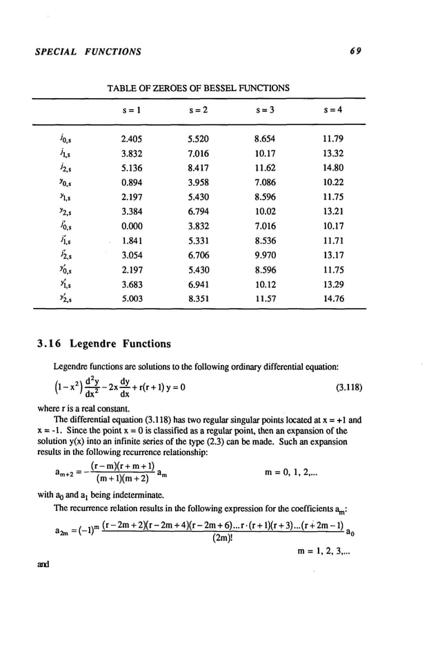
3.15 Zeroes of Bessel Functions
Bessel functions Jp(X)and Yp(x)have infinite number
of zeroes. Denotingthe th
root of Jp(x), Yp(x),J~(x)andY~(x)
by Jp,s, Yp,s,J’~,~, Y~,,, thenall the :zeroes
functions havethe followingproperties:
1. Thatall the zeroesof theseBess~lfunctionsare real if p is real andpositive.
2. Thereare no repeatedroots, exceptat the origin.
3. Jp.0=0forp>0
4. Theroots of Jp and Ypinterlace, such that:
P <Jp., <Jp+z.,<Jp.2<Jp+~.2
<Jp.~< "-
P<Yp,1<Yp+i,1
<Yp,2<Yp+l,2
< Yp,3<...
P- Jp,1 < Yp,1 < Yp,1 < Jp,1 < Jp,2 < Yp,2 < Yp,2 < Jp,2 < ...
5. Theroots Jp,1 and jp,1 can be bracketedsuch that:
~ <Jp,1 <42(p+l)(P
+3)
(3.115)
6. Thelarge roots of Bessel functions for a fixed order p take the followingasymptotic
form:
#,, s+7-
2
2
(3.116)
Theroots as given in these expressionsare spacedat an interval = ~. Theroots of
Jp, Yp, and J~ and Y~are also well tabulated, Ref. [Abramowitz
and Stegun]. All roots
of H(p
1), H~
z), Ip, I_p, andKpare complex
for real andpositive orders p.
Theroots of products of Bessel functions, usually appearingin boundaryvalue
problemsof the following form:
Jp(x) Yp(aX)-Jp(aX) Yp(x)
J~,(x) Y~(ax)-J~,(ax) Y;(x)= (3.117)
Jp(X) Y~(ax)- Sp(aX) Y;(x)
can be obtained from published tables, Ref. [Abramowitz
and Stegun].
Thelarge zeroes of the spherical Bessel functions of order n are the sameas the zeroes
of Jp, Yp, J~ and Y~with p = n + 1/2. Spherical Hankelfunctions have no real zeroes.](https://image.slidesharecdn.com/advancedmathematicalmethodsinscienceandengineering-hayek-230318001731-2b30ece5/85/advanced-mathematical-methods-in-science-and-engineering-hayek-pdf-83-638.jpg)
![CHAPTER 3 70
a2m÷l
= (_l)m(r-2m+ 1)(r-2m+ 3) ... (r -1) . + 2)(+ 4)... (r + 2m)
(2m+ 1)!
m=1,2,3 ....
Thus,the two solutions of eq. (3.118) become:
pr(X)= 1 r(r+l) x2 (r-Z)r(r+l)(r+3) X4
2! 4!
(r- 4)(r- 2)r(r +l)(r + 3)(r x6+
6~
+... +(_1)m[r - (2m- 2)]Jr - (2m- 4)]... r. (r +1)...(r + 2m- x2
m
+...
(2m)!
(3.119)
(r- 1)(r + 2) x3 (r- 3)(r- 1)(r + 2)(r 4)x5
qr(X):X +
3! 5!
_ (r-5)(r-3)(r-1)(r + 2)(r + 4)(r 6)7
7!
+...+(_l)m (r-2m+l)(r-2m-1)...(r- 1).(r + 2)...(r x2m+
1+... (3.120)
(2m+l)!
andthe final solution is givenas:
y = C,Pr(X)+ c2qr(x)
Theinfinite series solutions havea radius of convergence
p =1, such that Pr(X)and
qr(X) convergein -1 < x < 1. At the twoend points x = +1, both series diverge.
If r is an eveninteger = 2n, the infinite series in (3.119) becomes
a polynomial
degree2n, having the form:
22n(n!)
2
P2n(X)=(-1)n (2n)!
where
(4n - 1)(4n- 3)... 5.3.1 [ (2n)(2n-
Pzn(X)
(2n)! Lx2n 2(4n-1) x2n-2
((2n)!)2
1
n =0, 1, 2 .... (3.121)
+"" + (-1)n 2Zn(n!)Z(4n_
1)...5.3
Thesecondsolution q2nis an infinite series, whichdivergesat x = +1.
If r is an oddinteger =2n +1, then it canbe shown
that the infinite series (3.120)
becomesa polynomialof degree 2n+l, having the form:
22"(n!)
2
q2n+l= (-1)n (2n + 1)! P2~+~(x)
where](https://image.slidesharecdn.com/advancedmathematicalmethodsinscienceandengineering-hayek-230318001731-2b30ece5/85/advanced-mathematical-methods-in-science-and-engineering-hayek-pdf-85-638.jpg)
![CHAPTER 3 72
Notingthat:
dn (x2n~= (2n)(2n - 1)(2n - 2)...(n ~
dxn ~ /
dn (X2n-21 = (2n - 2)(2n - 3)...(n + n-2
dX
n ~,
then the polynomialform of Pn(X)in (3.125) becomes:
1 dn [ X2n--2 n(n-1) x2.-4
]
Pn 2~n! dxn X2n n 1!
2!
Examination
of the terms inside the square brackets showsthat they represent the
binomialexpansionof (x2 - 1)n. Thus,Pn(x) can be defined by the formula:
On(X)=
1 n
2On!
dx
n(x
2-1)° (3.126)
This representation of Pn(x) is knownas Rodrigues’ formula.
Theinfinite series expansionfor Qn(x)can be written in a closed formin terms
Pn(x). Assuming
that the secondsolution Qn(x)= Z(x) Pn(X),
z"2xPolx)-2(1-
x2)P:
z’
resulting in an indefinite integral for Z(x), such that the secondsolution Qn(x)becomes:
x
Qn(x): Pn(X)f(1-- ~12)P~2 (3.127)
SincePn(rl) is a polynomial
of degreen, then Pn(rl) canbe factored such that:
Pn(rl): (rl- rll Xrl
- ~2)...(rl - ~ln)
Thus,the integrandin (3.127) can be factored to give:
a o + bo + cl
+
c
n d~ d
2 d
n
... + ~-I. I- ~-...+
1-rl l+rl TI - 1"~1 1~- Tin (1~ - 1’11) 2 (1~- ~2)
2
where
1 1
ao= -~ bo = ~
d (1~- 11i)
2 d 1 2(’qRi - (1-1~2) R0I
ci=~rl(1-rl2)p~2<rl)rl=rli =~(1-~)Ri~ (1 -r12)2R~
where
Ri(rl) = Pn(rl).
rl-~h](https://image.slidesharecdn.com/advancedmathematicalmethodsinscienceandengineering-hayek-230318001731-2b30ece5/85/advanced-mathematical-methods-in-science-and-engineering-hayek-pdf-87-638.jpg)
![SPECIAL FUNCTIONS 73
Substitution of Pn(~)=(~ "/qi) Ri(~l) into (3.118),
(1-1)2) p~,_2nP~+ n(n + 1) Pnlrl
= (1)_ rh)[(1- 1)2)R~’-21)R~]+ 2[(1-1)2) R~-1)Ri]lrl = 1)i
Thus,R
i satisfies the differential equation:
=0
(1- .qZ) R;- nRilrl = ~1
i
hence:
Ci --0
1
(1-1)21P
11)=
i
Thus,the closed formsolution for Qn(x):
Qn(x): P,(x)-½1og(1-~l)+:’l log(l+rl)~ di ]
2
i__-~l1)-rh jrl :
=0
n
--’- Zx_x
2 Pn (x) log
i=l
Thus,the first few Legendrefunctions of the secondkind haveclosed form:
1 . . l+x
Qo="~ Po(x) l°g 1_-
~"
1 - - l+x
Q1 = "~ P1 (x)log ~
~ . l+x 3
Q2
= P2(x) log l_i~- ~
(3.128)
Q3=x.1p3(x)log.l+~X-~x :z 2
+--
l-x z 3
Thefunctions Qn(x)convergein the region Ixl < 1..
Anothersolution of (3.118), for integer valuesof r, whichis valid in the regionIxl >
canbe developed.Starting withthe recurrencerelationship withr =n, n = 0, 1, 2 ....
(n - m)(n+ m+
am+2= (m + 1)(m + 2) am m = 0, 1, 2
am+
2, am+
4, am+
6 .... can be madeto vanishif m= n or -n - 1 with the coefficient am# 0
to be takenas the arbitrary constant. For the integer value r = n, the recurrence
relationship can be rewritten as follows:](https://image.slidesharecdn.com/advancedmathematicalmethodsinscienceandengineering-hayek-230318001731-2b30ece5/85/advanced-mathematical-methods-in-science-and-engineering-hayek-pdf-88-638.jpg)
![CHAPTER 3 74
mCm-1)
(n-m+2)(n+m-1) am
thus
-(m-2)(m- 3)am_2 =
am-4= (n - m+ 4)(n + rn -
Setting m= n:
n(n-1)
an-2 = 2.(2n- 1)
m(m-1)(m- 2)(m- m
(n - rn+ 2)(n- m+ 4)(n+ m- 1)(n
n(n- 1)(n- 2)(n-
an-4 = ÷ ~~)(’~n_-~
Thus,thefirst solutioncanbewrittenas:
a.[x. n(n- 1)
Yl(x)
2. (2n- 1)
where
an canbeset to:
(2n- l)(2n- 3)...5.3.1
n~
n(n- 1)(n - 2)(n- xn_
, ]
xn-2q" 2" 4. (2n- 1)(2n- 3) -
suchthat yl(x) becomes
Pn(X),Settingrn = -n - 1, then:
(n +1)(n+
a_,_3 = ~ (2n + 3).2
(n+ 1)(n+ 2)(n+3)(n
a_n_5 = (2n+3)(2n+5).2~4 a_~_l
suchthat:
y~(x) = a_n_lLX-n-1
Settingthecoefficient:
n!
a_~_l= (2n+1)(2n- 1)... 5.3.1
(n + 1)(n +2) x_._3
2.(2n+3)
(n + 1)(n + 2)(n + 3)(n x_,_s]
q 2-4. (2n + 3)(2n + +""
thenthe second
solutionQn(x) can bewrittenin aninfinite series formwithdescending
powers
of x as follows:
n!
[
(n + 1)(n+ x_,_3
Qn(x)=,(2n+l)(2~--1)...5.3.1,x-n-~+ 2.(2n+3)
(n+l)(n+2)(n+3)(n+4) x_._s +...
1 Ixl >1 (3.129)
+ 2.4.(2n- 3)(2n +
TheWronskian
of Pn(x
) andQn(x)
can beevaluatedfromthe differential equation
(3.118).](https://image.slidesharecdn.com/advancedmathematicalmethodsinscienceandengineering-hayek-230318001731-2b30ece5/85/advanced-mathematical-methods-in-science-and-engineering-hayek-pdf-89-638.jpg)
![SPECIAL FUNCTIONS 75
W(Pn,Qn) = PnQ~- P~Qn: Woexp = l_x2W°
Usingthe form for Qnin (3.128), the following expressionapproachesunity as x --> +1:
W0
= Lim (1-x2)[P~Q:-P~Qn]-->l
x--~ +1
1
W(Pn’Qn ) 1-x2
3.17 Legendre Coefficients
Expanding
the following generating function by the binomialseries:
1.3 22
1 1
=l+l(2x-t)t+~--------~ (2x-t)2 t +
(1-2tX+ t2) 1/2 [1- t(2x- t)]
1/2
1-3-5...(2n- 1)
+~(2x- t)3t 3 +...+ (2x- t)nt n +... (3.130)
z.’~.t~ 2.4.6...2n
then onecan extract the coefficient of tn havingthe form:
1"3"5""(2n-
1) [xn~ [ 2(2n-
1)n(n-1)~~ ~
" 4 :~-’~n(n-
1)(n-
2)(n-xn_
4 +... ]
whichis the representation for Pn(x) given in eq. (3.125). Thus, the binomialexpansion
gives:
= ~t" Pn(x) (3.131)
1
(1-2tx+ t~) 1/~ n=0
Thegenerating function can be used to evaluate the Legendrepolynomialsat special
values. At x = 1:
1
1 l+t+t2+... = EtnPn(l) = Et
n
(l_2t+t2)~/z = 1_---~-= n=0 n=0
whichgives the value:
Pn(1) =
At x = -1:
1
(l+2t+t~)
1/~
1 1-t+t z t3+ ....
t" P~(-1) -1)"t
n
l+t
n=O n=O
whichgives the value:
Pn(-1)= (-1)
n](https://image.slidesharecdn.com/advancedmathematicalmethodsinscienceandengineering-hayek-230318001731-2b30ece5/85/advanced-mathematical-methods-in-science-and-engineering-hayek-pdf-90-638.jpg)
![CHAPTER 3 76
At x = 0, the generating function gives:
1
[
It2 + 1.3 t4 +...+ (_l)n
0÷t2),,2= 2.4
whichresults in a formulafor Pn(O):
Pn(0/-- (-1/"/21-3"5... (n- 1
/ = (_1/./2
2.4.6...n
1.3.5... (2n- 1) t2n +...1
2.4.6...2n
n~
2n[(n/2)!]
2
n : even
= 0 n=odd
Substituting t by -t in eq. (3.131) one obtains:
1
(l+2tx+t2)
l/2=n=~)Z(-1)nt"P"(x)=n=OZt"Pn(-x)
whichresults in the followingidentity:
en (-x)= (--1) n Pn(x)
Other forms of Legendrepolynomialscan be obtained by manipulatingeq. (3.131).
Letting x = cos 0, then:
1 1
(1-2tcosO+t2) 1/2 =(l_tei°f/2(1-te-i°f/2
1.3.5 t3e3iO 1.3...(2n- 1) tneni0
t ei o + 1.3 t2e2i0 + __
+...-~ ,...
= 1+ 2
2.4 2-4.6 2.4...2n
¯ I1 +t e_iO
+1 .__~3
t2e_2i
0 +1.3.5t3e_3i
0 +... +
2 2.4 2.4-6
1¯ 3...(2n
2¯ 4...2n-1)
tne_ni
o+...}
=l+t
{ ei° + e-i° } {~(
2 t- t2 e2iO -2i0,+"~+ ...
Thus,the coefficient of tn mustbe the Legendrepolynomial,the first fewof whichare
listed below:
Po= 1, P1(cos0) = cos
P2(cos 0) = ¼13cos20+ 1], P3(cos0) = -~ [5 cos30 + 3cos0]
and the Legendrepolynomialwith cosine argumentsis defined by:](https://image.slidesharecdn.com/advancedmathematicalmethodsinscienceandengineering-hayek-230318001731-2b30ece5/85/advanced-mathematical-methods-in-science-and-engineering-hayek-pdf-91-638.jpg)
![CHAPTER 3 8 0
1 -- 2COSO
eiu + e2iU]
1/2
~’~ ,~inu
= eiu/2(cos--~-~_ cos0)l/2 u < 0
Pn(cosO)
nfg
ei(u-x)/2 (cos u - cos 0)
1/2 u > 0
Equatingthe real and imaginaryparts, one obtains:
[ cos(u/2)
~ . r~/(cos
u- cos0)~2
u<o
2 cos(n u) Pn (cos0) = ,qz 1 sin(u/2)
n=O
[~
u>O
[ - sin(u/2)
.... r=/(cos u_cos0)~/2
u<0
2 ~ sin(n u)rn[cost0 = ~/z~ cos(u/2)
n=O
[~
u>O
(3.148)
(3.149)
Multiplyingeq. (3.148) by cos (n u) and eq. (3.149) by sin (n u) and integrating
on(0, rt), there results twointegrals for Pn(cos
-~ 0 cos(u/2)cos(n u)du+~ sin(u/2)cos(n u)dul
Po(cos
0)=
(cos
u-cos0)
1/2 ~ i
(3.15o)
0
¯
xf~ 0 sin(u/2)sin(n f cos(u/2)sin(n u)
Pn(COS0)=’-~’- - (COSU_COS0)I/2
(COS0_COSU)I/2
(3.151)
0
The integral representations of (3.150) and (3.151) are due to Dirichlet.
Addingand subtracting eqs. (3.150) and (3.151) one obtains:
1 0 cos(n + 1/2) u f sin(n + 1/2)
Po(cos0)=~--~
(cosu_cos0)l/2 (cos0_cosu)l/~
(3.15~)
0
0 cos(n - 1/2) u
sin(n - 1/2)
0 =~0(cos u - cos 0)1/~ du - ! (cos 0 - cos u)1/2 du (3.153)
Replacingn by n + 1 in the identity (3.153), and substituting the resulting identity in eq.
(3.152) one obtains:
pn(cosO) x/~ cos(n+l/2)u ~_~_.2~ sin(n+l/2)u
=’-~’o0 (cosu-cosO)~/2 du = /t ~0 (c°sO-c°su)~/2
(3.154)](https://image.slidesharecdn.com/advancedmathematicalmethodsinscienceandengineering-hayek-230318001731-2b30ece5/85/advanced-mathematical-methods-in-science-and-engineering-hayek-pdf-95-638.jpg)
![SPECIAL FUNCTIONS 81
Theintegral representations in eqs. (3.153) and (3,154) are due to Mehler.
3.20 Integrals of Legendre Polynomials
Oneof the most important properties of the Legendrepolynomialsis the
orthogon~lityproperty. Thefirst integral to be evaluatedis an integral of productsof
Legendrepolynomials.
Theintegral of products of Legendrepolynomialscan be evaluated by the use of
Rodrigues’formula(3.126):
+1 +1
Pn Pmdx = 2n+mn,m, dx----~- (x2 - 1) n x2 --1)m dx n>_m
-1 -1
wheren is assumedto be larger than m.
Integrating by parts, one can showthat:
+1
fPn Pm = n ;~ m (3.155)
dx 0
-1
If n = m, then the last integral becomes:
+1 +1
f Pn
2 dx=(-1)n(2n)’22n(n!)2
f(x2-1)ndx
-1 -1
Integratingthe last integral by parts, oneobtains:
+1
dx--2
2n + 1
(3.156)
-1
Theorthogonalitypropertycan also be provenby integrating the differential
equation. Thedifferential equationthat P,~ and Pm
satisfy for n ~ mcan be written in the
following form:
d--d~[(1- x2) P:] +n(n + 1) Pn
d-~-£ [(1- x2)P~] + m(m+ 1)Pm
Multiplyingthe first equationby Pro, the secondby Pn, and subtracting and integrating
the resulting equations, one obtains:](https://image.slidesharecdn.com/advancedmathematicalmethodsinscienceandengineering-hayek-230318001731-2b30ece5/85/advanced-mathematical-methods-in-science-and-engineering-hayek-pdf-96-638.jpg)
![CHAPTER 3 82
(3.157)
x
2
+ [n(n+l)-m(m+l)] fPn Pm dx=O
x
1
Integrating
eq. (3.157)byparts, thefollowing
expression
results:
x2
t
x2
[m(m+l)-n(n+l)] Prn dx=( 1-x2XPm P~-P,~ Pn (3.158)
Xl x
1
If onesets x1 = -1, x2 = +1,thenoneobtainsanotherproofof eq. (3.155).Substituting
eq. (3.142)into eq. (3.158),oneobtains:
x
2
jf PnPmdx = nPm
Pn-1- mPnPm-1+ (m- n) n Pm
(m-n)(m+ n+l)
x
1
Settingx
I = -1 andx:z = xin eq. (3.159)oneobtains:
x
~Pn nPmPn-I - mPn
Pro-1+ (m- n) n Pm
Pm
dx
(m- n)(m+ n +
-1
which
canbe evaluatedat x = 0 as follows:
0
fPndx =0 ifn is oddandis odd,
Pm in n in
-1
x2
In, n
x
1
(3.159)
m, n (3.160)
=0 if n is evenandmis even,n;~ rn
1 (-1)(n+m+l)/2
n! m!
= (m- n)(m+ n + 1) 2m+n-l[(m/2)!
((n - 2
if n is oddandmis even,n, m
1 (’1)(~+m+l)/~
n! m!
= (m-n)(m+n+l) 2m+n-~[(n/2)!((m_l)/2)!]
2
if n is evenandmis odd, n, m
SettingxI = x andx2 = 1 in ¢q. (3.159)oneobtains:
1
f 1 [mPnPro-1 - nPmPn-l-(m- n) xPn Pro}
jP. Pm
dx=(m-n)(m+n+l)
x
which
canbeevaluatedat x = 0 byusingthe results givenin eq. (3.161)since:
(3.161)
(3.162)](https://image.slidesharecdn.com/advancedmathematicalmethodsinscienceandengineering-hayek-230318001731-2b30ece5/85/advanced-mathematical-methods-in-science-and-engineering-hayek-pdf-97-638.jpg)
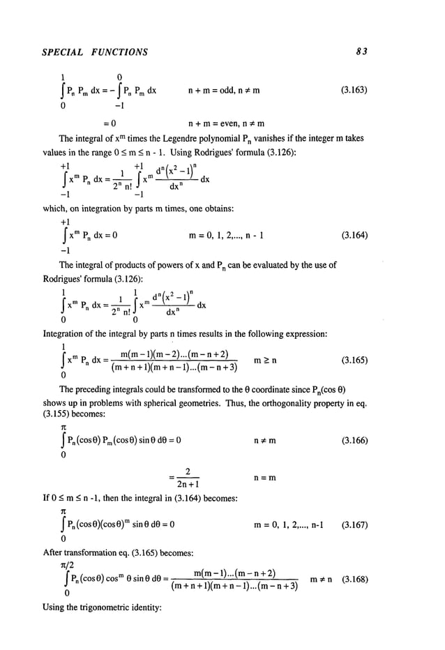
![CHAPTER 3 84
m(m-1)(m- sin2 0cosm_
3 0 +.. .. ]
sin (mO)-- sin 0 Imcosm-10
3!
then one can evaluate the followingintegral:
f Pn(cos0)sin (m0)d0 = f Pn(c.os0)Im cosm-1
0 0
m(m- 1)(m - 2) sine 0 cosm_
3 0
3!
m(m- 1)(m- 2)(m-
+ 5!
sin4 0 c0s
m-50 - ... sin 0 dO
If m< n, ~henthe highest powerof cos 0 is n - 1, thus usingthe integral of (3.167), each
term vanishesidentically, suchthat:
Pn(cos0) sin = 0
(m0)
0
Ifm >
hence,
f Pn(cos 0)sin (m0)dO
0
Ifm >
m=0, 1, 2 ..... n (3.169)
n and m+ n = eveninteger, then the integrandis an oddfunction in (0, ~), and
the followingintegral vanishes:
m+ n = even
n and m+ n = odd integer, then the integral becomes:
f Pn(cos 0) sin (m0)dO(m
- n +1)(m
- n + 3). .. (m
+ n -
(m-n)(m- n +2)...(m+
0’
Similarly one can showthat the integral:
~Pn(cos 0) cos (toO)sin 0
0
(3.170)
(3.171)
=0 m=0,1,2 ..... n-1
=0 m- n = odd integer > 0 (3.172)
-2
(m- 1) (m+
n = 0, m= even integer > 0
-2m(m- n + 2)(m - n + 4)...(m + n n >1
(m- n - 1)(m- n + 1)...(m + n m- n =eveninteger _>0
Thefollowingintegral can be evaluated by the use of the expressionfor Pn(cos 0)
terms of cos m0,given in eq. (3.132) as follows:](https://image.slidesharecdn.com/advancedmathematicalmethodsinscienceandengineering-hayek-230318001731-2b30ece5/85/advanced-mathematical-methods-in-science-and-engineering-hayek-pdf-99-638.jpg)
![SPECIAL FUNCTIONS 85
I Pn(cos O)cos (me)
0
=0 m<n
= 0 m + n = odd
r(m
+k+1/2)r(k+ 1/2)
= n=m+2k, k=O, 1,2 ....
r(k
+I)
r(m
++ 1)
Thefollowingintegral can be obtained by using the integral in (3.173):
I P" (cos0)sin m0sin0 dO: 91- I Pn(cos 0)[cos(m-1)0-cos(m+
0 0
(3.173)
=0 m>n+l
= 0 n - m= 0 or an eveninteger
mr(m+k - 1/2)r(k-1/2)
= n-m=2k-1, k=0,1,2 .... (3.174)
4 r(k+l)r(m +k+l)
Integrals involving products of derivatives of Legendrepolynomialscan be evaluated.
Starting withthe integral:
+1 +1
¯ I+1 ’
I(1-x2)P: P: dx:(1-x2)P: P~]_, - IPm{(1-xZ)P:}
-1 -1
+1
=n(n+l) IP~ P. dx=O
-1
n~m
_ 2n(n + 1) n=m
2n+l
Theprecedingintegral is an orthogonalityrelationship for P’n.
(3.175)
3.21 Expansions of Functions in Termsof Legendre
Polynomials
Thefirst function that can be expanded
in finite series of Legendrepolynomials
is
Pn(x). Starting with the recurrenceformula(3.138) for n, n-2, n-4 ..... one gets:
nPn= (2n- 1) x Pn- (n - 1)
(n - 2) P.-2 = (2n- 5) x P.-3 - (n - en-4
(n - 4) Pn-4= (2n - 9) x Pn-5-- (n - 5) P.-6
Thus,substituting Pn-2, Pn-4, into the expressionfor Pn, one obtains:](https://image.slidesharecdn.com/advancedmathematicalmethodsinscienceandengineering-hayek-230318001731-2b30ece5/85/advanced-mathematical-methods-in-science-and-engineering-hayek-pdf-100-638.jpg)
![CHAPTER 3 8 6
(n 1)
Pn
=x Pn-x n(n-2)
(n - 1)(n- (2n
-!9)P~-5-...1
n(n-2)(n-4)
(3.176)
Usingthe recurrenceformula(3.139)for P~:
P~= P,~-2+(2n- 1) P,~_~
P~-2 = P~-4 + (2n - 5)
V~-4 = P~-6 + (2n- 9)
andsubstitutingfor P~-2,P~-4
..... oneobtainsthefollowing
finite series for P~:
P~= (2n- 1) P,-1 + (2n - 5) P,-3 + (2n - 9) P,-s + ... (3.177)
Adifferent expansion
for P~canbedeveloped
fromthe recurrenceformula
(3.140):
xv~=xP~-2
+n
vo+(n-
1)P._2
xP~_~
=xP~-4
+(n-2)P.-2
+(n-
xP~-4
=xP~-6
+(n-4)P._,
+(n- 5)
Thus,a finite expansion
for x P~results:
x P,~=n Pn+ (2n-3) Pn-z+ (2n- 7) P,-4+ --- (3.178)
Differentiating
eq. (3.177)andsubstitutingfor P~_I,P~-z..... from(3.177) one
obtainsanexpansion
for P~’,havingthe followingform:
P~’= (2n- 3)(2n- 1.1) Pn-2+ (2n- 7)(4n- 2-3)
O.179)
+(2n- 11)(6n- 3-5) Pn-6+
Usingthe recurrenceformula
givenin (3.138):
(2n
+1)xV.(x)
=(n+1)Po+x(x)
+n
(2n+ 1) yPn(Y)= (n +1) Pn+~
(y) +n
andmultiplying
the first equationbyPn(Y)
andthe second
byPn(x),andsubtracting
resultingequalities,oneobtains:
(z.+1)(x
- y)P.
(x)P.
(y)=
(. +1)[Po
(y)Po+,
(x)-
P.
+n[P.(y)v._,(~)-
P.(x)Po_1(y)]
Thus,summing
this equationNtimes, there results:
N
(x-y) E(2n+ 1) P~(x) Pn(y)
n=0
N
= E (n + 1) [Pn (y) Pn+l(X)-Pn(x)P~+I(y}]-n[P~_l
(y)P~(x)-Pn-l(X)
n=0](https://image.slidesharecdn.com/advancedmathematicalmethodsinscienceandengineering-hayek-230318001731-2b30ece5/85/advanced-mathematical-methods-in-science-and-engineering-hayek-pdf-101-638.jpg)
![SPECIAL FUNCTIONS 8 7
The preceding summation formula is knownas Christoffel’s First Summation.
Toobtain an expansionin terms of squares of Legendrepolynomials,the formgiven
in (3.180) for x = y gives a trivial identity. Dividing(3.180) by x - y andtaking
limit as y -~ x, oneobtains:
N
Z(2n+I) Pn~(X)=(N+I) PN(Y
) PN÷~(x)--PN(X)PN÷~(Y)
n=0
y--~x x-y
= (N + 1)[PN(X
) P{~+l(X)-P~(x)PN+I(X)] (3.181)
Since LegendrepolynomialsPn(X)are polynomialsof degree n, then it stands
reason that one can obtain a finite sumof a finite number
of Legendrepolynomialsto
give xm. Expanding
xminto an infinite series:
xm---- Z ak Pk(x)
k=0
then multiplyingbothsides by Pl(X) and integrating both sides, one obtains:
+1
2/+1
j’x mPt(x) l =0, 1, 2.... (3.182)
al =T
-1
Examination
of the precedingintegral showsthat the constants aI for l < mdo not vanish
while aI = 0 for I > m(see 3.164). Ifm - l is an oddinteger in (3.182), then
integrandis an oddfunction of x, then:
al =0 if m- l =oddinteger
If m- l is an eveninteger, then using(3.165) oneobtains:
+1 1
212 + 1f Pl
1)f x mPl (x)
- j xTM
(x) dx = (2/+
a
I
-1 0
= (2/÷ 1). m(m- 1)(m- 2)...(m-l+ (3.183)
(m+ l +1)(m+l- l)...(m- /
Fromthe preceding argument,it is obviousthat only the LegendrepolynomialsPro,
Pm-2,Pm-4,’", do enter into the expansionof xm. Thus:
xm----
m!
~
~ (2m+1)t
,
1.3.5...(2m + 1)[(2m+ 1)Pm+ (2m- ~ 2-’~i~.~
+ (2m- 7) (2m+ 1)(2m- _ 1)(2m- 1)(2m- 3) Prn-6 + ...}
~.~ m-4 +(2m 11)(2m+ 23.3!
(3.184)
Thefirst fewexpansionsare listed below:
l=P0
’ x=P1
’
x2 2 1
=-~ P: +’~ Po](https://image.slidesharecdn.com/advancedmathematicalmethodsinscienceandengineering-hayek-230318001731-2b30ece5/85/advanced-mathematical-methods-in-science-and-engineering-hayek-pdf-102-638.jpg)
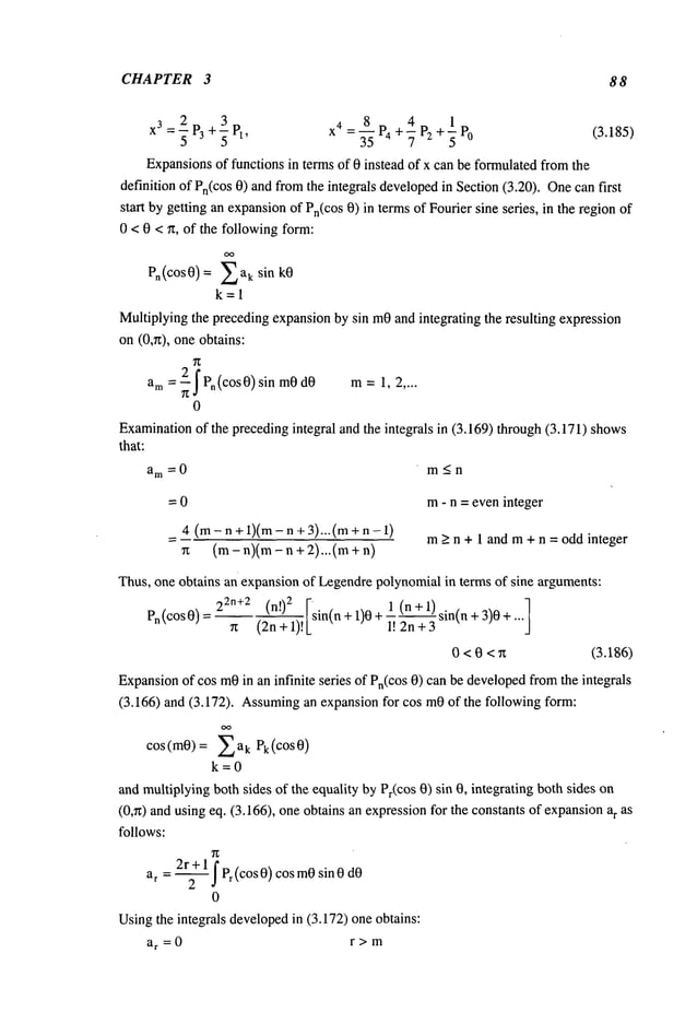
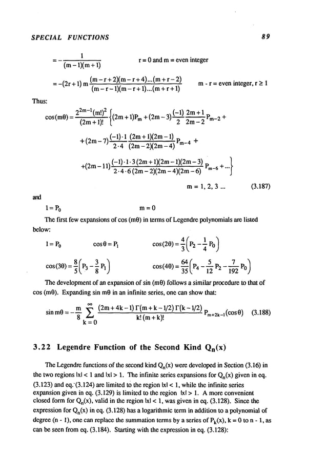
![CHAPTER 3 90
Qn(x) = ½ p,(x)
log~_--~-
w._l
and substituting Qn(x)into the differential equation(3.118), one obtains after
simplification:
t" - ax j dx
Usingthe expansionfor (d Pn)/(dx) fromeq. (3.177), the right side of eq. (3.189)
becomes:
2[(2n- I) P.-I + (2n - 5) P.-3 +(2n - 9) P.-5 + -.-]
Assumingthat:
k<(n-l)/2
k=0
and substituting Wn.
I into eq. (3.189) and equating the coefficients of Pk, one obtains
expressionfor ak as follows:
2n - 4k - I
ak = (n - k)(2k + k = 0, I, 2 .... k < (n-l)/2
Thus,the function Wn.
I can be expressedin terms of a finite series of Legendre
polynomials as:
2n-7
2n-I p + 2n-5 P.-3 ~
P.-5 +... (3.190)
w.-,=
~.--i--
~-.-i 3-(n-I) 5.(n-2)
Aformula, similar to Roddgues’
formulafor Pn(X), can be developedfor Qn(x).
Starting with the binomialexpansionof (x2 - l), one obtains:
1 I n+1 I n+2 1
(x,-_1)n÷’--x
1!2o-’’2t x2°-°÷’’"
Integrating the precedingseries n + l times, the followingexpressionresults:
.~.~"".~
(5-’-~÷~
=(n+1)(n+2)... (2n- 1)(2n)(2n
xrlrl ~1~
q
[ (n+l)(n+2)x-"-~ (n+l)(n+2)(n+3)(n+4)x-n-’
¯ x-"-i + 2(2n +3) + 2.4-(2n +3)(2n+ +""
Comparison
of the precedinginfinite series with the series expansionfor Qn(x)for Ixl >
in eq. (3.129) results in the followingformfor Qn(X):](https://image.slidesharecdn.com/advancedmathematicalmethodsinscienceandengineering-hayek-230318001731-2b30ece5/85/advanced-mathematical-methods-in-science-and-engineering-hayek-pdf-105-638.jpg)
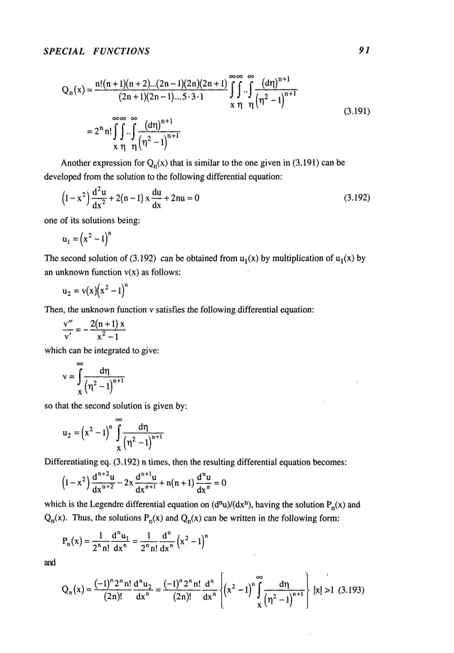
![CHAPTER 3 92
Theconstants were adjusted such that ul") and u~
n) become
Pnand Qn,respectively.
Anintegral for Qn(x)valid in Ixl< 1 canbe obtainedfrom(3.193), resulting in the
¯ following
integral:
(-1)’n2nn, dn
n! dr
I
Qn(x)= (2n)! dx" l-x2) (1_TI2)
n+l
A generating function representation can be formulatedfrom the following binomial
expansion:
1 i t + __ + x~ +""
valid for < 1
x_t=~’+x ~- x3 +...
Substituting for tn by a series of Legendrepolynomialshaving the form(see eq.
3.184):
2n(n!)2 f 2n+l p "t’+
tn = ~ l(2n + 1) Pn (t) + (2n -
+(2n- 7) (2n2.41)(2n
-1)en-4 (t)+ ..
Then:
(3.194)
1 r’o r,, 1 re +L +3_ ] lr8r, 4 +± ]
3Po -F P3 5P1 "F’~L ~" 4+~’P2 5Po
xn ’ [(2n +I)!L
collectingtheterms
that multiplyP0, P1, P2..... Pn, then the coefficient of’Pn becomes:
(2n + 1) 2n(n[)2
I (n + 1)(n +2)x-n-3 ]= (2n +1) Qn(x
)
(2n+1)!
x-"-x ÷ 2. (2n + / +""
Thus:
OO
1= E(2n. +l) po(t)Qn(x)
Ixl >1 (3.195)
x--t
n---0
Theexpansiongiven in (3.195) leads tO an integral representation for Qn(X).
Multiplyingboth sides by Pm(t)and integrating on (-I, 1) one obtains:
+1
Q.(x) --1 f P.(t) Ixl >1 (3.196)
-2 Jx-t
-I
Thelast integral is knownas the Neumann
Integral.](https://image.slidesharecdn.com/advancedmathematicalmethodsinscienceandengineering-hayek-230318001731-2b30ece5/85/advanced-mathematical-methods-in-science-and-engineering-hayek-pdf-107-638.jpg)
![SPECIAL FUNCTIONS 93
3.23 Associated Legendr,e Functions
AssociatedLegendrefunctions are solutions to the followingdifferential equation:
2 m2 1
(I- x2~d’Y- 2x d-~-Y + [n(n + 1)- 1_--~ y=0 (3.197)
] dx2 Ox L
wheremand n are both ~ntegers.
Substituting:
i~ eq. (3.197)results in a newdifferential equation:
~d2u_
(1- 2(m
÷1)x~÷I"
-re)In
÷m
÷~)u
x
2
/ dx
2
Differentiating Legendre’seq. (3.118) mtimes, one obtains:
m+2 Jm+l
Equations(3.198) and (3.199) are identical, thus, the solutions of (3.198) are ~h
derivative of the solutions of (3.118). Thus,the solution of eq. (3.197) becomes:
1)~[.-z-r
dm~’n
~Qn
]
y={x
a-
Define:
~’2
-- (~-1)
~dm~’~ ~~1
dx
TM
Q~m
=(x2-1)m/~"" d~Q" Ixl >1 (3.201)
dx
TM
as the associated Legendre functions of the first and second kind of degree
n and order m, respectively.
Define:
T~
m= (-1)m(1- x2)’~ droP" Ixl <1 (3.202)
dx
m
as Ferret’s function of the first kind of degree n and order m. It may be
convenientto define Pn
mand Q~in the region Ixl < 1 as follows:
P.~ =T.
m, Ixl <l
dx
~
Ixl <1 (3.203)
Usingthe expression for Pn(x) given by Rodrigues’formula, then:](https://image.slidesharecdn.com/advancedmathematicalmethodsinscienceandengineering-hayek-230318001731-2b30ece5/85/advanced-mathematical-methods-in-science-and-engineering-hayek-pdf-108-638.jpg)
![CHAPTER 3 94
2n n! dxm ÷n
Ixl >1 (3.2o4)
(2n)! _ m~[x
n-m (n-m)(n-m-l)
2n n! (n - m- 1)! (xz 1)
xn-m.-2
2(2n-1)
+ (n - m)(n - m- 1)(n - m- 2)(n - 3)n- m-4]
2.4-(2n-- 1)(2n-3)
x -...
It can be seen from(3.205) that p,m= 0 if m>_n - 1. Theterms containedin the
brackets of (3.214) represent a finite polynomial
of degreen -
Alisting of the first fewAssociatedLegendrefunctions is given below:
=(x2-1) P?--0
(3.205)
P~ = 3x(xZ-1)
~2 P~ =3(x2-1) P~=O
p33=15x(x2- 1)
3/2
P~ = ~(7x~ - 3x)(x2-1)
~
If n = m,then:
. _ (2n)! .1)9/2
P~- 2nn-~.(x
2 Ixl >1
Anotherexpression for P~, similar to (3.200), can be developedin the form:
1 (x-lh~ ¢ r,
PZ=2
ln_m)!(777+
)
] 1
(3.206)
(-1)" (1-x)~/~ ~
2" (n - m)! kl-’-~x J d-’~-[(x- 1)"-’~(x + 1)"+m]
(3.207)
3.24 Generating Function for Associated Legendre Functions
Usingthe generating function for Pm(X)
given in (3.131)
1
= ~tnPn(x)
(1-2xt+@n=O
anddifferentiating the equality mtimes, one obtains:
1.3.5....(2m- 1) m d~P.
(1-2xt+t2) m+~ =n=m Ztn dxm](https://image.slidesharecdn.com/advancedmathematicalmethodsinscienceandengineering-hayek-230318001731-2b30ece5/85/advanced-mathematical-methods-in-science-and-engineering-hayek-pdf-109-638.jpg)
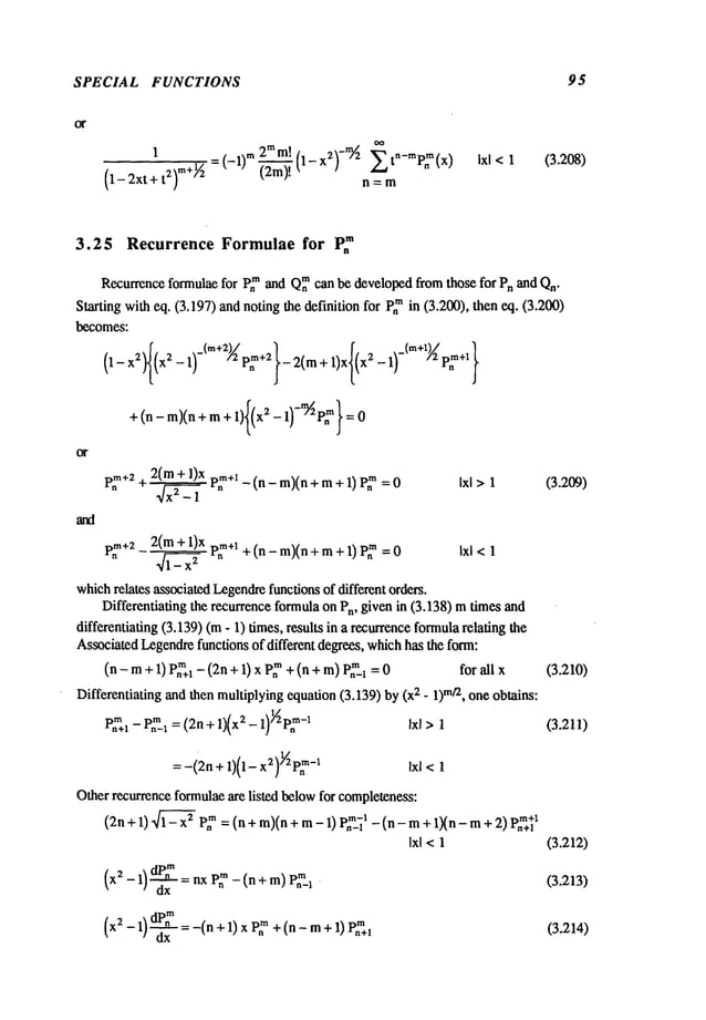
![CHAPTER 3 96
Dm+l = x(n_m+l)p~+l _(n+m+l)p
~ Ixl> 1 (3.215)
~x
2-1 . n+l
(n+ m) ~x~_ 1 p~-I _
m
- P~+a
- x P~ Ixl>1 (3.216)
(n - m+ 1) ~ - 1 P~
-I = x P~
- P,~-I Ixl >1 (3.217)
More
recurrenceformulae
can befoundin Prasad,Volume
II.
3.26 Integrals of Associated Legendre Functions
Integralsof products
of associated
Legendre
functionsarepresented
in this section.
Startingwiththedifferential equation
that associated
Legendre
functions
of different
degreesandthe sameorderp.mandP~satisfy, andmultiplying
the first equationbyp~m,
the secondequationby P~,subtractingthe resulting equationsandintegratingthe
resultingequationon(-1, +1),oneobtains:
+1
[r(r +1)- n(n+1)] J" prmpn
TM dx=
-1
= , L .x It xj
-~- ’L’ --~x-v"~ =0 n,r
-I
Starting
withthedifferentialequations
thatassociated
l.~gendre
of thesame
degree
and
differentorders
P~and
P~satisfy, and
multiplying
thefirst equation
byP~,the
second
equation
byP~,subtracting
theresultingequations
and
integrating
theresultant
equality,one
obtains:
(m~-V)f~,_x~X=
~xk’ ’ ~x~
" dx=O
--1 --
m~k
The
integralof squares
of associated
Legendre
functions
canbeobtained
byusingthe
+1
~(p~)2 dx= (n+m)~. ~p.mp~,.
(n m)!
+1
(n + m)! ~+’~ d~’’~ (x
2
(n-m)!22n(n!) 2 ~ d~X--~(X2--1}"~-m~ -1)ndx
--1 ’
Inte~afing~eNst integral by pros mtimes gives:
definition of P~.
+1](https://image.slidesharecdn.com/advancedmathematicalmethodsinscienceandengineering-hayek-230318001731-2b30ece5/85/advanced-mathematical-methods-in-science-and-engineering-hayek-pdf-111-638.jpg)
![SPECIAL FUNCTIONS I01
(k) xEy"+(4-x) xy’+/4kZx4 +xZ-2X+5/y=04
(1) xEy"-(2X E +x) y’+xy=O
(m) xEy" +(2xE-x)y’+ xEy=O
(n) xZy"+(2xE +x) y’+(5x z +x-4) y=O
10. Show
that the substitution for g(x) in eq. (3.70) by the followingexpression:
g(x) =(f(x))
b-a
results in the followingdifferential equation.
d~u+F(l-2b) f’ f"ldU-IE rE+b E aE~) 2 0
dx" L f - f’ J dx
t f -
- u =
whosesolution becomes:
U= (f(x))b Zp(f(x))
where
p2 = r2 + a
2
11. Show
that the substitution for g(x) in eq. (3.70) by the followingexpression:
g(x) = 7
results in the followingdifferential equation:
dx
EdEu2a f_.’ du +I(f_~(fE -r E +1 + a)-
f dx L f k. 4
whosesolution becomes:
U = ~ faZp(f)
withp2=r2 +a
2.
f" 3(f")
E lf"’l
a f 4 (f,)2 ~-~7-]
u=O
Section 3.10
12. Show
that the BesselCoefficientsJ,(x) givenin eq. (3.75) satisfy Bessel’s
differential equation
(3.1).
13. Obtainthe recurrenceformulaegivenin eqs. (3.13) to (3.16) by utilizing
generating function.](https://image.slidesharecdn.com/advancedmathematicalmethodsinscienceandengineering-hayek-230318001731-2b30ece5/85/advanced-mathematical-methods-in-science-and-engineering-hayek-pdf-116-638.jpg)
![SPECIAL FUNCTIONS 103
Section 3.16
23. Assuming
a trial solution for Legendre’sequation, having the following form:
~’ a x
Y= L, n
n=O
obtain the twosolutions of Legendre’sequationvalid in the regionIxl > I (see eq.
3.129).
24. Showthat:
P~(1) = n(n+l) and p~(_l) = (_l)n_l n(n+
2 2
25. Obtainthe first three Qn(x)by utilizing the formgivenin (3.128).
Section 3.17
26. Showthat:
Pzn
(0)
=(-1)
n
=0
(2n)!
n=O,1,2 ....
n=O,1,2 ....
by the use of the generating function.
27. Provethat the Legendrecoefficients of the expansionof the generating function
satisfy Legendre’s
equation.
Section 3.18
28. Showthat:
(2n + 1)(1- 2) P~ =
n(n + l)(Pn_
1 - P~
+I )
29. Showthat:
(1- x2)(P~)2= ~xx [(1-x2)P~P~] + n(n+ 1)Pn
2
Section 3.19
30. Provethe first equality in (3.142) byusingthe integral representationfor P~(x)
(3.145).](https://image.slidesharecdn.com/advancedmathematicalmethodsinscienceandengineering-hayek-230318001731-2b30ece5/85/advanced-mathematical-methods-in-science-and-engineering-hayek-pdf-118-638.jpg)
![SPECIAL FUNCTIONS 105
Section 3.22
39. Showthat:
(n + 1)[QnPn+
~ - Qn+IP,,]= n[Qn_~P
n -QnPn_~
]
40. Showthat:
2n +1
Pn+lQn-~- Pn-~Qn+ln(n + 1)
41. Showthat:
~ ....
1)2[pnQn- Pn+aQn+l]
(1-x)[P,~+,Qn+a- P:Q,~] : (n
42. Showthat:
¯
[
2n+l
+ 1)(2n + 3)Qn+4
+ ...]
x-~-I = 1.3.5 ...(2n - 1) (2n + 1)Q
n - (2n + 5) ~ Q~+z+ (2n + 9) (2n
n!
(Hint: Differentiate (3.195) n timeswithrespect to t and set t--](https://image.slidesharecdn.com/advancedmathematicalmethodsinscienceandengineering-hayek-230318001731-2b30ece5/85/advanced-mathematical-methods-in-science-and-engineering-hayek-pdf-120-638.jpg)
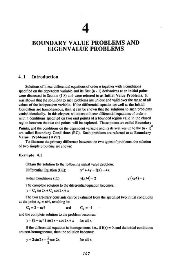
![BOUNDARY VALUE AND EIGENVALUE PROBLEMS 109
y = C1sin.~- x + C2cos~]~ x 3.;~0
Yo= C~x+ C4 3. =0
Satisfying the boundary
conditions at the twoend points yields:
y(O) = 2 =0 an d C 4= 0
y(n/4) = C1 sin~- ~ = 0 and C3=0
Thelast equation on C1leads to twopossible solutions:
yo=O
For a non-trivial solution, i.e., C1~ 0, then sin ~/~ ~/4 = 0, whichcanbe satisfied
if the undetermined
parameter3. takes anyone of the followinginfinite discrete
number
of possible values, i.e.:
3.1 = 16.12, 3.2 = 16.22, 3.3 = 16- 32 ....
In other words,Xn= 16n
2 n = 1, 2, 3 .... are the Eigenvalues which satisfy the
following Characteristic Equation:
sin ~ { = 0
Thus,the solution, whichis nontrivial if 3. takes any oneof these special values, has
the following form:
y = C
1 sin4nx n=1, 2, 3 ....
whichis non-unique,since the constant C1is undeterminable.
The functions ¢, = sin 4nx are knownas Eigenfunctions. Thevalue ~ = 0 gives
a trivial solution, thus it is not an Eigenvalue.
(ii) If 3. doesnot takeanyoneof those values,i.e., if:
3., 16n
2 n =1, 2 ....
then
C1 =0
andthe solution vanishesidentically.
4.2 Vibration, WavePropagation or Whirling of Stretched
Strings
Considera stretched loadedthin string of length L andmassdensity per unit length p
in its undeformed
state. Thesiring is stretched at its endby a force To,loadedby a
distributed force f(x) andis beingrotated about its axis byan angularspeed= to, as shown
in Fig. 4.1.](https://image.slidesharecdn.com/advancedmathematicalmethodsinscienceandengineering-hayek-230318001731-2b30ece5/85/advanced-mathematical-methods-in-science-and-engineering-hayek-pdf-123-638.jpg)
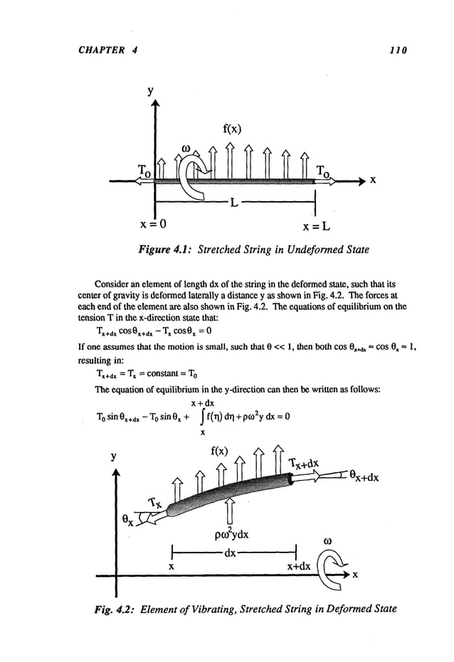
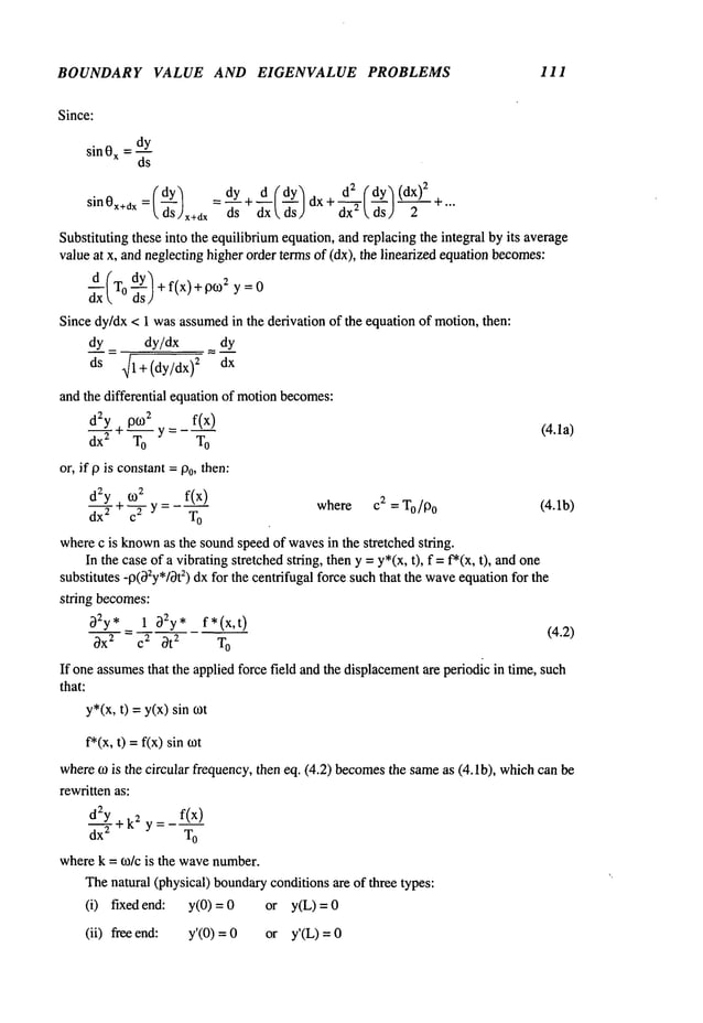
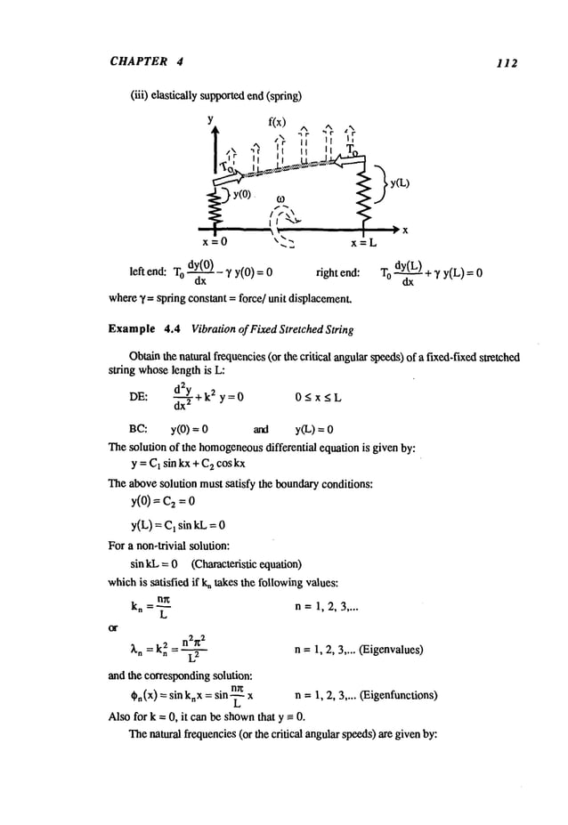
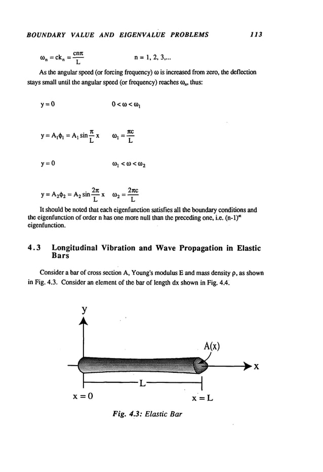
![CHAPTER 4 114
x x+dx
Ax [~d×-----~ A
Undeformed State: ~~
~"l’:: U x+dx
DefonnedState: Fx~f’:~ ~-’ £!i~:Ii::ii ~ Fx+dx
Fig 4.4: Element of a Vibrating Elastic Bar in Longitudinal Motion
Eachcross section is assumedto deformby u*(x,t) along the axis of the rod as shown
Fig. 4.4. Let u*(x,t) be the deformationat location x and at time t, then the deformation
at location x+dxandt is:
u~+dx--- u~ + -~- dx
then the elastic strain as definedby:
deformation u~ + (o~u */o~x) dx -
strain e = _=
original length dx o~x
and the correspondingelastic stress using Hooke’slaw becomes:
stress o" = E 030*
Thetotal elastic force F on a cross-section canbe computed
as:
&*
F=Aa=AE--
Theequation of equilibrium of forces on an elementsatisfies Newton’ssecondlaw:
F,÷d,- F~+ f * (x,t):ctx = mT~-
dX
x (A u*]10x)2+
_ A*
3xl~ ~x ) +~-’~, "-~x )’~"- ""-P ~-~-~-dx-f*(x,t)dx](https://image.slidesharecdn.com/advancedmathematicalmethodsinscienceandengineering-hayek-230318001731-2b30ece5/85/advanced-mathematical-methods-in-science-and-engineering-hayek-pdf-128-638.jpg)
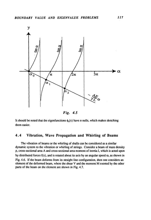
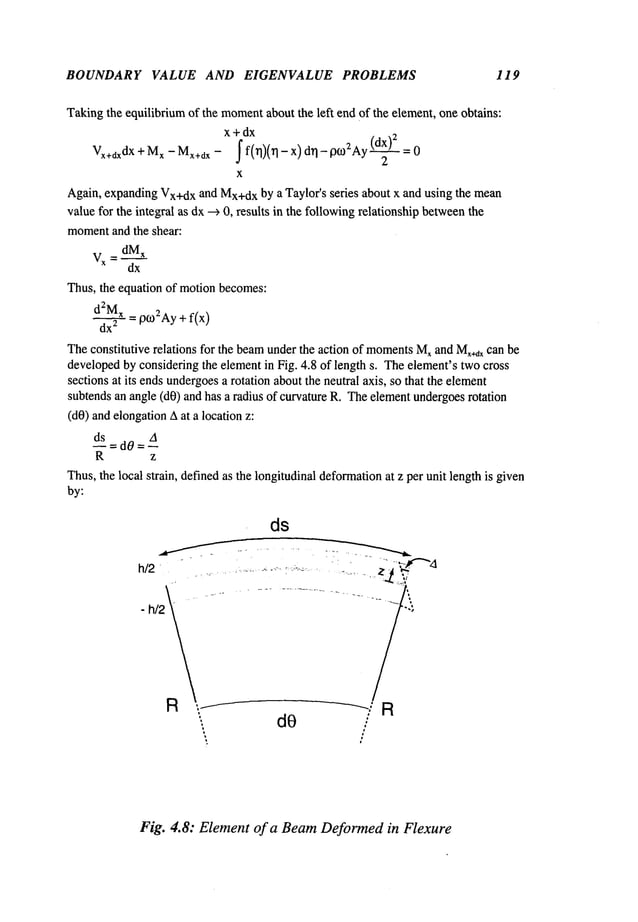
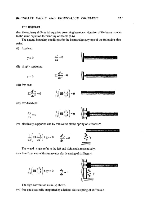
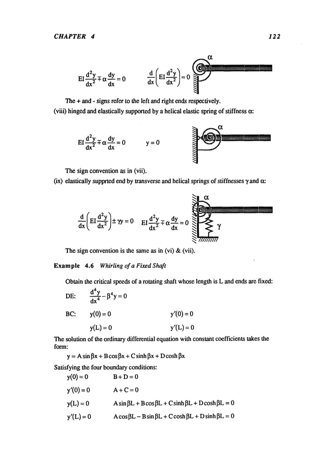
![BOUNDARY VALUE AND EIGENVALUE PROBLEMS 123
Y
c~os~
For a non-trivial solution, the determinantof the arbitrary constants A, B, Cand Dmust
vanish,i.e.:
0 1 0
1 0 1
sin ~L cos ~L sinh ~L
cos[~L -sinl]L cosh~L
1
0
=0
cosh
sinh ~L
Thedeterminantreducesto the followingtranscendental equation:
coshIXcosI.t = 1 (CharacteristicEquation) where I.t = [~L
The roots can be obtained numericallyby rewriting the equation:
cosIX=1/coshIX
wherethe twosides of the equality can be sketchedas shown
in Fig. 4.9.
Theroots can be estimated from the sketch aboveand obtained numericallythrough
the use of numerical methodssuch as the Newton-Raphson
Method.Thefirst four roots
of the transcendentalequationare listed below:
I.to=0 IX1= 111L
= 4.730
IX2= ~2
L = 7.853 IX3= 113
L = 10.966
Denoting
the roots byI~, then I]n = l-tn/L, n =0, 1, 2 .... andthe eigenvaluesbecome:
~,, =l]~
4 =~tn~/L
4 n=1, 2, 3 ....
Onecan obtain the constants in terms of ratios by using any three of the four equations
representing the boundaryconditions. Thus, the constants B, C, and Dcan be found in
terms of Aas follows:
B sinh~t~- sinl.t, D
~"=cosh~t. - cosIX~
=-’X=~
C
A
which,whensubstituted in the solution, results in the eigenfunctions:](https://image.slidesharecdn.com/advancedmathematicalmethodsinscienceandengineering-hayek-230318001731-2b30ece5/85/advanced-mathematical-methods-in-science-and-engineering-hayek-pdf-137-638.jpg)
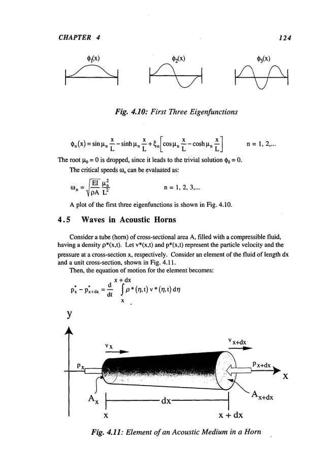
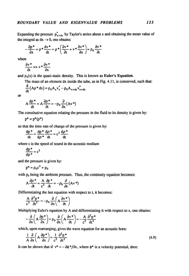
![BOUNDARY VALUE AND EIGENVALUE PROBLEMS 127
Y
y=l
x=O
I
Oo(X)
Fig. 4.12: First Three Eigenfunctions
Theroots of the characteristic equation(Section 3.15) and the corresponding
eigenfunctions become:
k0L = 0
klL = 3,832
k2L = 7.016
k3L = 10.17
*0 =1
*1 =J0 (3.832x/L)
’2 =J0 (7.016x/L)
*3 :J0 (10.17x/L)
Aplot of the first three modes
is shown
in Figure 4.12.
X
4.6 Stability of Compressed Columns
Consider a columnof length L, havinga cross-sectional area A, and moment
of
inertia I, being compressed
by a force P as shown
in Fig. 4.13.
If the beamis displacedlaterally fromout of its straight shape, then the moment
at
any cross-section becomes:
M
x =-py
which, whensubstituting Mxin Section (4.4) gives the following equation governingthe
stability of a compressed
column:
d2 (" dZy "] d2y_
d--~-/El d--~-/ + P ~ - f(x)
(4.13)
Equation(4.13) can be integrated twiceto give the followingdifferential equation:
EI d2~y+ Py= ff f(rl) drl drl +1 +C2
x (4.14)
dx
2](https://image.slidesharecdn.com/advancedmathematicalmethodsinscienceandengineering-hayek-230318001731-2b30ece5/85/advanced-mathematical-methods-in-science-and-engineering-hayek-pdf-141-638.jpg)
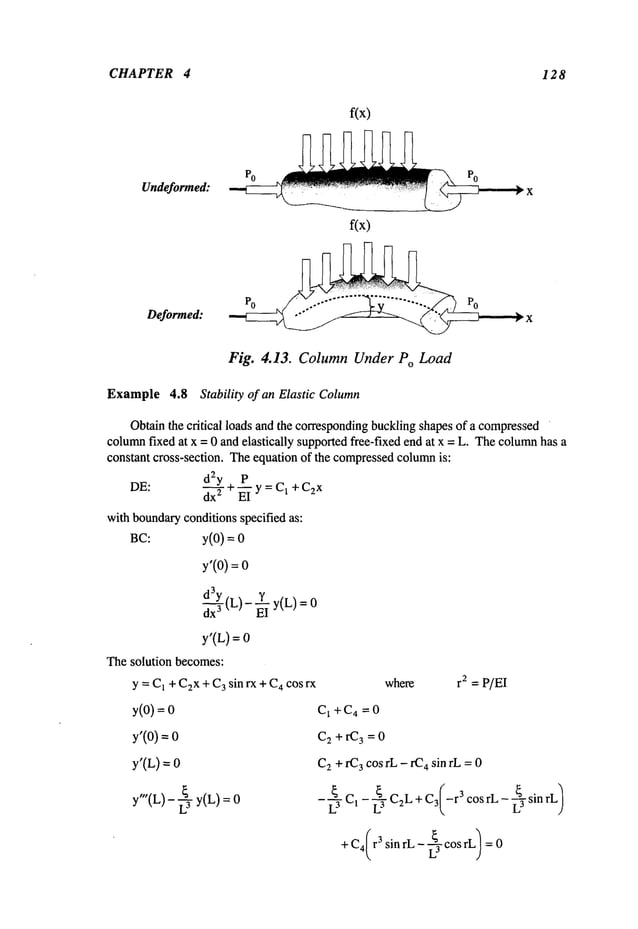
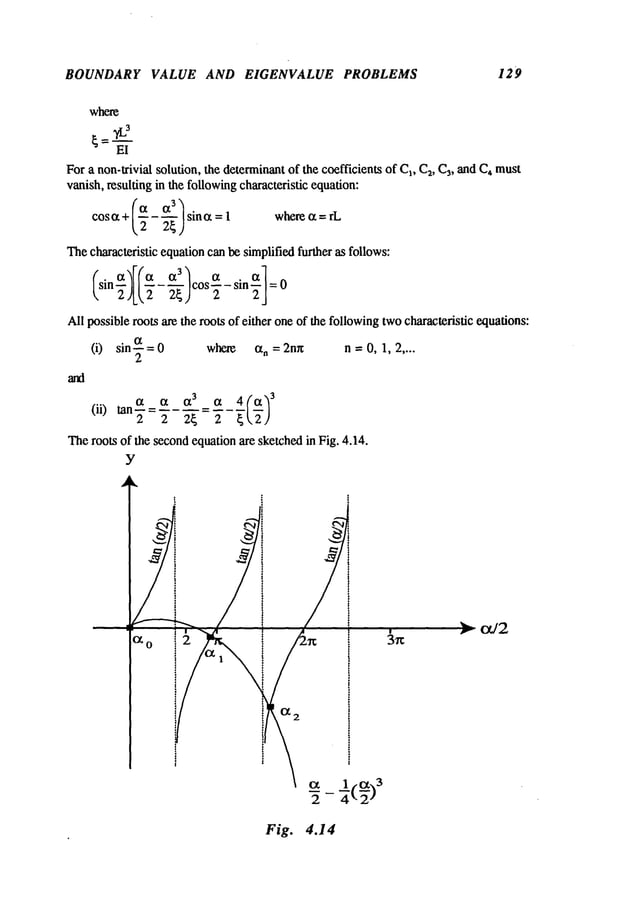
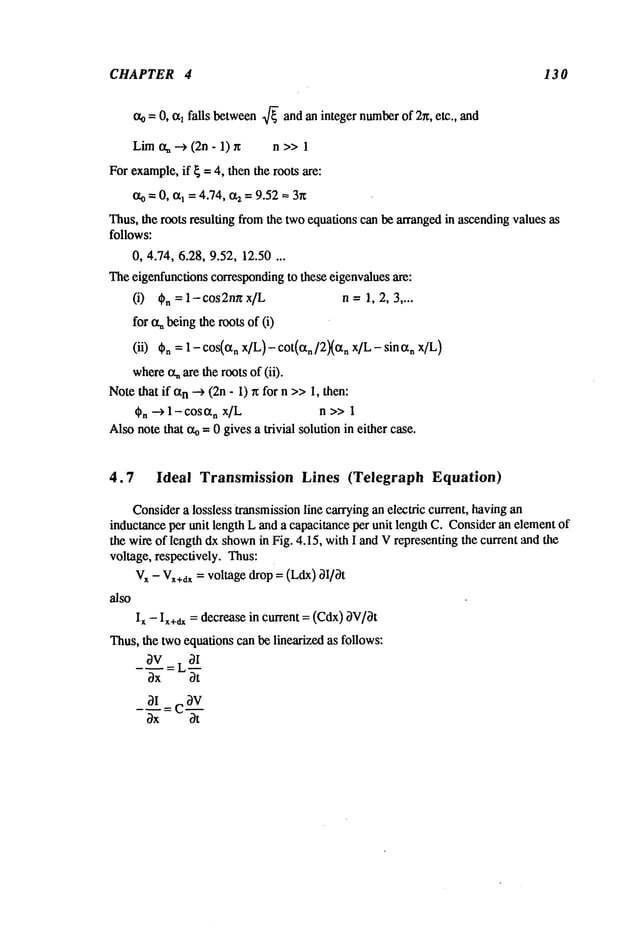
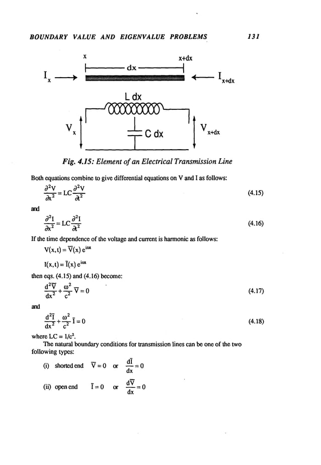
![BOUNDARY VALUE AND EIGENVALUE PROBLEMS 133
wherec is the shear soundspeedin the bar def’medby:
cm= G/p
If t’*(x,t) = f(x) sin tot and0*(x, t) =0(x) sin tot, theneq. (4.20)
ld(j d0)+k20= f
J dxk dxJ GJ
If the polar moment
of inertia J is constant, then:
d20 + k20 = f
dx
2 GJ
Thenatural boundaryconditions take one of the following forms:
(i) fixed end 0=0
(ii) flee end = GJ-~ = 0 ~
(iii) elastically supportedendbyhelical spring
The+ and- signs refer to the BC’sat the right andleft sides.
(4.21)
(4.22)
4.9 Orthogonality and Orthogonal Sets of Functions
Theconceptof orthogonalityof a pair of functions fl(x) and f2(x) can be defined
throughan integral over a range [a,b]:
b
(f,(:,), f2(x))=~ f, (x)
a
If thefunctions
fl(x)andf2(x)areorthogonal,
then:
Definethe norm
of f(x) as:
b
N(f(x)) =J" [f(x)]2dx
a
Aset of orthogonal
functions{fi(x))i =1, 2 .... is one whereevery pair of functions
of the set is orthogonal,i.e. a set {f,~(x)i is an orthogonal
set if:](https://image.slidesharecdn.com/advancedmathematicalmethodsinscienceandengineering-hayek-230318001731-2b30ece5/85/advanced-mathematical-methods-in-science-and-engineering-hayek-pdf-147-638.jpg)
![BOUNDARY VALUE AND EIGENVALUE PROBLEMS 135
L
2 f sin (n~x)sin (rn~x) dx~m
n
LJ L L
0
Jo(Oq~
x/L)
(ii) Theset g,(x)= Ljx(ctn)/~]~ n = 1, 2, 3,...in < x < L
constitutesanorthonormal
set, where
{gn(x)}
is orthogonal
withw(x)
L
2 ~x Jo(Ctn x]L)J0(ct mx]L)dx = 8nm
L2J12(~n)
where
~aretherootsof J0(ct,) --
e~X
(iii) Theset gn (x) n-- 0, 1,2.... in -r~ <x < ~
constitutesanorthonormal
set where:
1 fe~X~ 1 ~e~Xe-~mx
~
ei~xdx = ~-n dx = 8m~
4.10 Generalized Fourier Series
Consider
an infinite orthonormal
set {go(x)}orthogonal
over[a,b]. Then
onecan
approximate
anyarbitraryfunctionF(x)definedon[a,b] in termsof a finite series of the
functionsgin(x).Let:
N
F(x) = clg~c2g2 + .. . + c~
qgN= 2 Cm
gm(x) (4.23)
m=l
thenmultiplying
the equalitybygn(x),n beinganyinteger number
1 _<< N,
andintegratingon[a,b], oneobtains:
b N b
~F(x) gn(x)dx: 2cmfgm(x) gn(x)dx=cn
a m=la
sinceeverytermvanishes
because
of the orthogonality
of the set {g~(x)},exceptfor the
termm= n. Thusthe coefficient of the expansion,called the FourierCoefficient,
becomes:
b
Cm
=JF<x)
gin(x)
dx
a
andF(x)canberepresented
bya series of orthonormal
functionsas follows:](https://image.slidesharecdn.com/advancedmathematicalmethodsinscienceandengineering-hayek-230318001731-2b30ece5/85/advanced-mathematical-methods-in-science-and-engineering-hayek-pdf-149-638.jpg)
![CHAPTER 4 13 6
F(x)- ~’~, gm(x) F(~l) gm(~l) a<x<b (4.24)
m=l
Theseries representationof (4.24) is called the Generalized
FourierSeries
corresponding
to F(x). Thesymbol
~, usedfor the representation
insleadof anCxluality,
refers to the possibilitythat the series may
not converge
to F(x)at some
pointor points
in [a,b]. If anorthonormal
set {gn}extendsto aninfinite dimensional
space,thenN
extendsto infmity.
TheGeneralizedFourier Series is the best approximationin the meanto a
functionF(x). Consider
a finite number
of an orthonormal
set as follows:
n
~kmgm(x)
m=l
thenonecanshow
that the best least squareapproximation
to F(x) is that where
cm= k~.
Thesquareof the errorJ between
thefunctionF(x)andits representation,
definedas:
hi n q2
j=I/F<x)-
Ekmg
<x)
/ ax_>0
a/ m=l /
mustbe minimized.
Thesquareof the error is expanded
as:
J=~F2 dx-2 Ekm~F(x) gm(x)dx+ kmgm(X) ) dx
a m=l a al_m = 1 J/r=l J
Sincethe set {g~.}is anorthonormal
set, thenJ becomes:
b n n
J=~F2dx-2 ~Cmkm+ 2k2m->O
a m=l m=l
b n
a
b n n
a m=l m=l
Tominimize
J, whichis poSitive, thenonemustchooselq~= cm.
n
~., Cmgm(X)
m=l
is the best approximationin the meanto the function F(x).
b n
~F2 dx> ~c2~
a m=l
Thus,theseries:
SinceJ ~ 0, then:](https://image.slidesharecdn.com/advancedmathematicalmethodsinscienceandengineering-hayek-230318001731-2b30ece5/85/advanced-mathematical-methods-in-science-and-engineering-hayek-pdf-150-638.jpg)
![BOUNDARY VALUE AND EIGENVALUE PROBLEMS 137
Theaboveinequality is not restricted to a specific number
n, thus:
b ~
~ F 2 dx > ~cZ~ (4.25)
a m=l
b
Since J-Fz dx is finite, then the Fourier Coefficients Cmmust constitute a
a
convergent
series, i.e.:
m~
A necessaryandsufficient conditionfor an orthonorrnalset { g,(x)} to be completeis
that:
b ~
~F2(x) : ~C~m
a m=l
Thegeneralized Fourier series representing a function F(x) is unique. Thustwo
functionsrepresentedbythe samegeneralizedFourier series mustbe equal, if the set { g. }
is complete.
If an orthonormal
set is completeandcontinuous, andif the generalizedFourier series
correspondingto F(x) is uniformlyconvergentin [a,b], then the series converges
uniformlyto F(x) on [a,b], if F(x) is continuous.
Similar expansionsto eq. (4.24) can be developed,if the orthonormalset {g,(x)}
orthonormalwith respect to a weightingfunction w(x) as follows:
F(X)= ~Cmgm(X
)
m=l
where
= f w(x) F(x)gm(X)dx
c
m
a
b
~w(x) gm(X)gn(X)dx
a
(4.26)](https://image.slidesharecdn.com/advancedmathematicalmethodsinscienceandengineering-hayek-230318001731-2b30ece5/85/advanced-mathematical-methods-in-science-and-engineering-hayek-pdf-151-638.jpg)
![CHAPTER 4 138
4.11 Adjoint Systems
Consider
the linear nth orderdifferential operatorL:
Ly=[a0(x)d--~+al(x)~+...+a,_~(x ) +an(X ) y=0 a<x<b (4.27)
where
ao(x
) doesnot vanishin [a,b] andthe coefficientsai, i = 0, 1, 2 .... n are continuous
anddifferentiable(n-i) times, then definethe linear th order differentia! operator K
:
d
n d
n-1 dn-2
Ky= (-1)n d--x~ [a0 (x) y] + (-1)n-I dxn_
~ [al(x)y] + (-1)n-2 dxn:2 [a2(x)y
]
d [an_l(x) y]+ an(X)
(4.28)
dx
as the Adjoint operator to the operator L. Thedifferential equation.:
Ky =0
is the adjoint differential equationof (4.27).
Theoperator L andits adjoint operator Ksatisfy the followingidentity:
v Lu - u Kv = ~x P(u, v) (4.29)
where
n-ldmuln-m-1 dk
P(u,v) = m~__
0d-~[ k=0E(-1)k d--’~ "(an-m-k-l(x) V) (4.30)
Equation (4.29) is knownas Lagrange’s Identity.
ThedeterminantA(x)of the coefficients of the bilinear formof °) v~) becomes:
A(X)
= -+[a0(x)]
n (4.31)
whichdoes not vanish in a < x < b.
Integrating (4.29), one obtains Green’sformulahaving the form:
b Lu
dx =P(u,v)
J’(v - u (4.32)
a a
Thedeterminantof the bilinear formof the right side of (4.32) becomes:
~(a) 0~(b)l
=A(a)
A(b)
=[ao(a)
a0(b)]n
If the operators K= L, then the operator L and K are called Self-Adjoint.
Asan example,take the general secondorder differential equation:
Ly=a0 (x) y" + a~(x) y’ 2 (x)y =
then the adjoint operator Kbecomes:](https://image.slidesharecdn.com/advancedmathematicalmethodsinscienceandengineering-hayek-230318001731-2b30ece5/85/advanced-mathematical-methods-in-science-and-engineering-hayek-pdf-152-638.jpg)
![BOUNDARY VALUE AND EIGENVALUE PROBLEMS 139
Ky=(a0y) -(aly ) +a2y
=aoy"+ (2a~ - al) y’ + (a[’- a~ +a2)y
whichis not equalto Lyin general andhencethe operator L is not self-adjoint. If the
operator Lis self-adjoint, then the followingequalities musthold:
a1 = 2a~- a
1 and a2 = a~ - a~+ a~
whichcan be satisfied by one relationship, namely:
a0 = al
whichis not true in general. However,
one can changethe secondorder operator L by a
suitable function multiplier so that it becomes
self-adjoint, an operationthat is valid only
for the secondorder operator. Hence,if one multiplies the operator L
1 by an
undetermined
function z(x), then:
LlY = z Ly
so that L1is self-adjoint, then eachcoefficient is multipliedby z(x). Sincethe condition
for self-adjoincyrequires that the differential of the fast coefficient of L equalsthe second,
then:
(z ao) = z
whichis rewritten as:
z" a1 - a
0
z a
o
Thefunction z can be obtainedreadily by integrating the abovedifferentials:
l_~exp[ ~ ai(rl) drll = p(x)
Z=ao<x)
Usingthe multiplier function z(x), the self-adjoint operator L1can be rewritten as:
L1y = p(x) y"+ ~p(x) az( x) p(x
o( ) + ao(x) Y
= Id(pd~+q]
Ldx i, dxJ
where
: exp[~al(rl) d~]
p(x)
q(x) = a2(x) (4.33)
ao(x ) ¯
Thus,any secondorder, linear differential equation canbe transformedto a formthat
is self-adjoint. Themethod
used to changea secondorder differential operator L to](https://image.slidesharecdn.com/advancedmathematicalmethodsinscienceandengineering-hayek-230318001731-2b30ece5/85/advanced-mathematical-methods-in-science-and-engineering-hayek-pdf-153-638.jpg)
+ (-1)~-l[ply(n-1)](~-1)+ ...-[p~_ly’]’ + p~y=
a <x _<b (4.34)
4.12 Boundary Value Problems
Asmentioned
earlier, the solution of a systemis uniqueiff n conditions on the
function y andits derivatives up to (n - 1) are specified at the endpoints a and b. Thus,
general form of non-homogeneous
boundaryconditions can be written as follows:
n-1
Ui(Y)= X[~iky(k)(a)+[~iky(k)(b)]=~’i i= 1,2,3 ..... n (4.35)
k=0
wherecq,, I~, and Ti are real constants. Theboundaryconditions in (4.35) must
independent. This meansthat the determinant:
det[l~ij, ~ij] #0
Thenon-homogeneous
differential equation (4.27) and the non-homogeneous
boundaryconditions (4.35) constitute a general formof boundaryvalue problems.
necessaryand sufficient.condition for the solution of such problemsto be unique, is that
the equivalent homogeneous
system:
Ly = 0
Ui(y)--- i =1, 2..... n
has onlythe trivial solution y -- 0. Thus,an (n)~ orderself-adjoint operatorgivenin eq.
(4.27) has n independentsolutions {yi(x)}. Thus, since the set of n homogeneous](https://image.slidesharecdn.com/advancedmathematicalmethodsinscienceandengineering-hayek-230318001731-2b30ece5/85/advanced-mathematical-methods-in-science-and-engineering-hayek-pdf-154-638.jpg)
![BOUNDARY VALUE AND EIGENVALUE PROBLEMS 141
conditionsgivenin eq. (4.35) are independent,
then the solution of the differential eq.
(4.34) can be written as:
n
y = yp(x)+ ECiYi(X)
i=l
whereC
i are arbitrary constants. Since the set of n non-homogeneous
boundary
conditions in eq. (4.35) are independent,then there exists a non-vanishing
uniqueset
constants [Ci] whichsatisfies these boundary
conditions.
Ahomogeneous
boundaryvalue problemconsists of an nt~ differential operator and a
set of n linear boundary
conditions,i.e.:
Lu=0
Ui(u
)
:. 0 i ----1,2.... n
Anadjoint systemto that defined aboveis defined by:
Kv =0
Vi(v)=0 i=1,2 .... n
(4.27)
(4.35)
(4.28)
(4.36)
wherethe homogeneous
boundaryconditions (4.36) are obtained by substituting the
boundary
conditions Ui(u) = 0 in (4.35) into:
P(u, V)[a
b =0 (4.37)
withthe bilinear formP(u, v) beinggivenin (4.30). If the operator L is a selfoadjoint
operator, i.e. if K=L, then the boundary
conditions can be shown
to be identical, i.e.:
Ui(u)= Vi(u) (4.38)
Example 4.10
Forthe operator:
Ly=a0(x)y"+al(x)y’+a2(x)y=0
the adjoint operator is givenby:
Ky=(aoy ) -(aly ) +a2y=0
Thebilinear formP(u, v) is given by:
b
,
b
P(u,v) la= ulalv.-(aov)’l+u [aoV]la
(i)
a~xSb
Considerthe boundarycondition pair on u given by:
u(a) = and u(b) =
andsubstitution into (4.37) results in the following:
u’(a0V)la
b=u’(b)[ao(b)
v(b)]-
u’(a)[ao(a
) v(a)] =](https://image.slidesharecdn.com/advancedmathematicalmethodsinscienceandengineering-hayek-230318001731-2b30ece5/85/advanced-mathematical-methods-in-science-and-engineering-hayek-pdf-155-638.jpg)
![CHAPTER 4 142
Since u(b) = 0 then u’(b) is an arbitrary constant. Similarly since u(b) = O,
u’(a) is also arbitrary. Forarbitrary constants u’(a) andu’(b), the relation
satisfiedif:
v(a) = and v(b) =
(ii) If u’(a) and u(b) =
then one obtains the followingwhensubstituted into P(u,v) =
u’(b)[ao(b) v(b)]-u(a)Ial(a ) v(a)-(ao(a ) v(a))’]
Since u’(a) = 0 then u(a) is arbitrary. Similarly, since u(b) = O, then u’(b)
arbitrary. Thus,the boundaryconditions Vi(v) = 0 are:
al(a) v(a)-[ao(a ) v(a)] =
v(b)=
4.13 Eigenvalue Problems
Aneigenvalueproblem
is a systemthat satisfies a differential equation withan
unspecified arbitrary constant ~, and satisfying a homogeneous
or non-homogeneous
set of
boundaryconditions.
Consider a general form of a homogeneous
eigenvalue problem:
Ly + ~,My= 0 (4.39)
Ui(y)=0 i= 1,2 .....
whereL is given by (4.27) and the boundaryconditions by (4.35). ~Theoperator Mis
m
th order differential operatorwherem<n and~, is an arbitrary constant.
A general formof a self-adjoint homogeneous
eigenvalue problemtakes the
following form:
Ly + ~,My= 0 a < x _<b
U~(y)= i =1,2 ..... 2n (4.40)
whereL and Mare linear self-adjoint operators of order 2n and2mrespectively, where:
Ly= E(
-1)k ~.-’~’/dky] (4.41)
k=O L "" J
My= E(-1)kd--~ qm_kd--
j n>m
k=O
)~ is an undeterminedparameter, and Ui(y) = 0 are 2n homogeneous
boundaryconditions
having the formgiven in (4.35).](https://image.slidesharecdn.com/advancedmathematicalmethodsinscienceandengineering-hayek-230318001731-2b30ece5/85/advanced-mathematical-methods-in-science-and-engineering-hayek-pdf-156-638.jpg)
![CHAPTER 4 144
b
, ,Ib̄lr b
- J(u’v’
- v’u’)
dx 0
Iluv"-
vu,,)--
ov
a ,a a
b
(u rv-ru)dx=
v
a
which
provesthat the eigenvalue
problem
is self-adjoint. Toestablish that the problem
is alsopositivedefinite,substituteLandM
into eq. (4.44):
- (u’)2dx:-
(u’)2
a a a a
b b
rum=f m2 dx>O since r(x) >
which
indicatesthat theeigenvalue
problem
is also positivedefinite.
4.14 Properties of Eigenfunctions of Self-Adjoint Systems
Self-adjointeigenvalue
problems
havefewpropertiesuniqueto this system.
(i) Orthogonal eigenfunctions
If the eigenvalue
problem
is sclf-adjoint, thenthe eigenfunctions
areorthogonal.
Let
~ and~,~be anytwoeigenfunctions
corresponding
to different eigenvalues
7%
and
~.m,theneachsatisfiesits respective
differentialequation,
i.e.:
L~n + ~,nM(~n = an~ L~m + ~,mM~m = 0
wheren ~ mand7%# Z=.
Multiplying
the first equationby~m,the second
by~,, subtractingthe resulting
equations
andintegratingthe final expression
on[a,b], oneobtains:
b b b
a a a
Sincethesystem
of differential operatorsandboundary
conditions
is self-adjoint, and
since7%
~ L=,thentheintegral:
b
~M~.= n # m
dx 0 (4.45)
a
=N
n n=m](https://image.slidesharecdn.com/advancedmathematicalmethodsinscienceandengineering-hayek-230318001731-2b30ece5/85/advanced-mathematical-methods-in-science-and-engineering-hayek-pdf-158-638.jpg)
![BOUNDARY VALUE AND EIGENVALUE PROBLEMS 145
is a generalized formof an orthogonality integral, with N~being the normalization
constant.
(ii) Real eigenfunctions and eigenvalues
If the systemis self-adjoint andpositive definite, then the eigenfunctionsare real and
the eigenvaluesare real andpositive. Assuming
that a pair of eigenfunctionsand
eigenvaluesare complex
conjugates, i.e. let:
On= u.(x) + ivn(x
) ~n = Otn+ i~n
0; = un(x)-ivn(x) X~= a, -i[3
n
then the orthogonalityintegral (4.45) results in the followingintegral:
b
(x- x*)J0nM0:
dx=
a
Sincethe eigenvaluesare complex,i.e. ~3~~ O, then:
b
JO
MO
dx:o
a
whichresults in the followingreal integral:
b
~ (unMu. dx = 0
vnMvn)
+
a
Invokingthe definition of a positive definite system,bothof thes~integrals are
positive, whichindicates that the only complex
eigenfunctionpossible is the null
function, i.e,, un = v~ = O. Onecan also showthat the eigenvalues ~ are real and
positive, Starting out withthe differential equationsatisfied by either ¢nor 0~, i.e.:
L~n + ~LnMOn =0
and multiplyingthis equation by 0~ and integrating over [a,b], one obtains an
expression for ~:
~’n= tXn+ i~n=
b b
~O;L~n
dx ~(unLun + vnLvn)
a a
b b
~ O:MOn
dx ~ (unMtln + vnMvn)
a a
Sincethe systemis positive definite and the integrandsare real, then these integrals
are real, whichindicates that 13. =- 0 and ~ is real. Sincethe systemis positive
definite, then the eigenvalues~ are also positive. Having
established that the
eigenvaluesof a self-adjoint positive definite systemare real and positive one can
obtain a formulafor ~. Starting with the equation satisfied by On:
IL~n + ~,nMOn = 0](https://image.slidesharecdn.com/advancedmathematicalmethodsinscienceandengineering-hayek-230318001731-2b30ece5/85/advanced-mathematical-methods-in-science-and-engineering-hayek-pdf-159-638.jpg)
![CHAPTER 4 146
and multiplyingthe equationby ~n and integrating the resulting equation on[a,b],
one obtains:
b
f ~,I_@, dx
~’n = - ~ > 0 (4.46)
~nM~n dx
a
(iii) Rayleigh quotient
Theeigenvalues ~ obtained fromeq. (4.46) require the knowledge
of the exact form
of the eigenfunction~n(x), whichof course could havebeenobtained only if ~,
already known.However,one can obtain an approximate upper boundto thee
eigenvaluesif one can estimate the form of the eigenfunction. Definethe iRayleigh
quotient R(u) as:
b
~
uLu dx
a (4.47)
R(u) = -
~
uMudx
a
whereu is a non-vanishingcomparisonfunction. It can be shownthat for a self-
adjoint and positive definite system:
~1 = min R(u)
whereu runs through all possible non-vanishingcomparisonfunctions. It can also
be shown
that if u runs throughall possible comparison
functions that are
orthogonal
to the first r eigenfunctions,i.e.:
b
~uM~i
= = 1, .... r
dx 0 i 2, 3
a
then
Z,~+~
=min
R(u)
Example 4.12
Obtain approximatevalues of the first two eigenvalues of the following system:
y"+Z,y= 0 0<_x_<~
y(0) = y(r~) :
For this system, L = d2/dx
2 and M= 1 and hencethe systemis self-adjoint and also
positive definite. Solvingthe problemexactly, one can showthat it has the fi)llowing
eigenfunctions and eigenvalues:](https://image.slidesharecdn.com/advancedmathematicalmethodsinscienceandengineering-hayek-230318001731-2b30ece5/85/advanced-mathematical-methods-in-science-and-engineering-hayek-pdf-160-638.jpg)
![BOUNDARY VALUE AND EIGENVALUE PROBLEMS 147
%(x)= sin (nx)
~’n= n2 n= 1,2,3 ....
Usingthe definition of L andM,onecan show
that Rayleigh’squotientbecomes:
b b
R(u)=a _a
b b
a a
where
rain [R(u)l=~,1 = 1.0O
Onecanchoosethe followingcomparison
functionswhichsatisfies u(O)= u(x)
andhas noothernull between
0 andx, approximating
¢1(x):
~x/~t 0<x_<~/2
ut(x) =[1-x/n ~/2_<x_<~t
whichis not a propercomparison
function, becauseu" is discontinuous.TheRayleigh
quotientgives:
x]2
~ (1/~)2 dx÷~ (-l]x) 2 dx
0 ~/2 12
Rl(u)
=+~/2 ~ =~"=1.23>1.00
0 ~/2
If onewasto usea comparison
functionthat is at least oncedifferentiable,again
approximating
~(x) suchas:
ul(x)=x(~-x)
~(~-2x)
2 dx
0 10
R1(u) = = ~-T= 1.03> !.00
~x2(~
- x)2 dx
0
which
representsanerror of 3 percent.
It canbeseenthat R(u)> ~,~= 1, i.e. it is anupperbound
to ~ andthat the closer
comes
to sin x, the closer the Rayleigh
quotientapproaches](https://image.slidesharecdn.com/advancedmathematicalmethodsinscienceandengineering-hayek-230318001731-2b30ece5/85/advanced-mathematical-methods-in-science-and-engineering-hayek-pdf-161-638.jpg)
![CHAPTER 4 148
Toobtainanapproximate
valuefor Lz= 4.00, onecan usea comparison
function
u2(x)that hasonemore
null thanul(x), e.g.:
u2(x) = 4x/n 0 _< x <
= 2- 4x/~t if4 _<x < 3r¢4
=-4 + 4x/x 3r¢4< x < r~
whose
u’ is not continuous.Substitutingu2(x)into R(u), oneobtains:
R2(u)= 4.86 > 4.00
whichhasa 21 percenterror. Usinga comparison
functionwhichis at least onc~
differentiable,
e.g.:
us(x) = x) 0 _<x
= _<
x_<
thenthe quotientgives:
Rz(u)= 4.053> 4.00
One
shouldnote that the error is down
to 1.3 percentfor a comparison
functionwhich
is
at least once
differentiable.
4.15 Sturm-Liouville System
TheSturm-Liouville
(S-L)system
is a specialcaseof (4.40)limitedto a se~ond
order
eigenvalue
problem.
Starting witha general,second
order operatorwithanarbitrary
parameter."
a0(x)y" + al(x) y" + a2(x)y + Z,%(x) a_<x_<b (4.48)
thenonerewriteseq. (4.48)in a self-adjointformbyusinga multiplierfunctionto the
differentialequation
in theform:
~tCx)= p(x)
a0(x)
where
p(x) = exp(~al(x)/a0(x)dx)
thenthe differentialequation
canberewrittenin theform:
[p(x) y’] + q(x) y + Lr(x) a _<x_<b (4.49)
where
q(x) = as(x) p(x)/a0(x
)
r(x) = a3(x) p(x)/ao(x
)
Thetwogeneralboundary
conditionsthat can beimposed
ony(x) maytake the form:](https://image.slidesharecdn.com/advancedmathematicalmethodsinscienceandengineering-hayek-230318001731-2b30ece5/85/advanced-mathematical-methods-in-science-and-engineering-hayek-pdf-162-638.jpg)
![BOUNDARY VALUE AND EIGENVALUE PROBLEMS 149
~ly(a) + ~2y(b)+ ~3Y’(a)+ {x4Y’(b)= 0
[~y(a)+ ~2y(b)+[~3y’(a)+ [~4y’(b)
Thedifferential equation(4.49) is self-adjoint, i.e. the operators:
L = d Vpd 1 + q and M= r(x) are self-adjoint.
dxl_ dx.]
In order that the systemhas orthogonaleigenfunctionsand positive eigenvalues, the
problemmust be self-adjoint and positive definite (see 4.42 to 4.44). Theproblem
self-adjoint,if:
b ,
,
ib
, [b
f{uI(pv’ ) +qv]-vI(pu’ ) +qu]}dx=P(v,u)= p(x)[uv’-vu
a ,a a
= p(b)[u(b) v’(b) - u’(b) v(b)]- p(a)[u(a) v’(a)- (4.50)
Eliminatingin turn y(a) and y’(a) fromthe boundaryconditions, one obtains:
y~y(a) + y23y(b)- 7~4y’(b) = 0
~/13y’(a)+ ?x=y(b)+"h4Y’(b) (4.5 la)
Eliminatingin turn y(b) and y’(b) one obtains:
"Y~4y(b)
+"Y14y(a)
+ Y34y’(a)
V~4y’(b)
+?~2y(a)- ?z3y’(a) = 0 (4.51b)
where
~/ii = ~i[~j -- aj[~i = --Tii i, j =1, 2, 3, 4
If onesubstitutes for y(a) andy’(a) from(4.51) into the self-adjoint condition(4.50),
obtains:
[p(b,-p(a, ~][u(b)v’(b,-u’(b)v(b,]
whichcanbe satisfied if:
~/~4p(a)=~/13P(b)
wherethe identity:
~’l~’z3+ ~’34~q2
= ~3"/z4wasused.
(i) If~,13 = O, then ~/u =O, and (4.51) becomes:
y[o/- ~ y’(b)=
~’23
y(b)+~1__~.4
.... = 0
whichindicates that:
y(a)+~’3._~.4
,, , =
~,~4YI,a/
y(a)-~’~3 ,- ,
~’~2y ~a)=
(4.52)](https://image.slidesharecdn.com/advancedmathematicalmethodsinscienceandengineering-hayek-230318001731-2b30ece5/85/advanced-mathematical-methods-in-science-and-engineering-hayek-pdf-163-638.jpg)
![BOUNDARY VALUE AND EIGENVALUE PROBLEMS 151
Theeigenfunctions~o of the systemare thus orthogonal, satisfying the following
orthogonalityintegral, eq. (4.45), i.e.:
b
f r(x) (~n (X) (X)dx = n ~ m (4.57)
a
=N
n n=m
In order to insure that the eigenvaluesare real and positive, the systemmustbe positive
definite (see 4.44). Thus:
b b
~u Ludx =~ uI(pu’)’ + qu] dx =~ [-p(x)(u’)2 + 2] dx <0
a a a
b b
fuMudx=fru2 dx>0
a a
Thus,it is sufficient (but not necessary)that the functionsp, q andr satisfy the following
conditionsfor positive-definiteness:
p(x) >
a<x<b
q(x)_< (4.58)
r(x) >
to guaranteereal andpositive eigenvalues.
It can be shown
that the set of orthogonaleigenfunctions of the proper S-Lsystem
with the conditions imposedon p, q and r constitute a completeorthogonalset and hence
may
be used in a GeneralizedFourier series.
Example 4.13 Longitudinalvibration of a free bar
Obtainthe eigenfunctionand the eigenvaluesfor the longitudinal vibration of a free
bar, giving explicitly the orthogonality conditionsand the normalizationconstants.
y"+~,y = 0 0<x<L
y’(0) = y’(L) =
Thesystemis S-Lformalready, since it can be readily rewritten as:
d--~Cd-~-Y/+
~,y:0
where
p=l q=0 and r=l](https://image.slidesharecdn.com/advancedmathematicalmethodsinscienceandengineering-hayek-230318001731-2b30ece5/85/advanced-mathematical-methods-in-science-and-engineering-hayek-pdf-165-638.jpg)
![BOUNDARY VALUE AND EIGENVALUE PROBLEMS 153
Thesystemis in S-L form, with:
p(x) = 1 > 0 q(x) = 0 and r(x) 2 > 0
whichindicates that it is a proper S-Lsystem.
Thesolution to the differential equation(see 3.66) can be written in termsof Bessel
functionsof fractional order:
y=w/~’{C1J
1//4(’v~-x2/(2L2)) + C2J_1~(~/~ x2/(2L2))}
Since:
= = Lim I-U-~,zl x
) x-+ O x-+
Lira ~ J_~ ~ = Lira 4xl ~]
then both homogeneous
solutions arefinite at x = O. Satisfying the first bound~y
conditions yields C~= 0 and satisfying the secondbound~y
condition yields:
whichresults in the followingcharacteristic equation:
Jg(~) = where a =
Thenumberof ~e roots %of ~e preceding ~anscendental equation ~e infinite wi~
%= 0 being the first root. Thus,the eigenfunctions and the eigenvalues become:
~n(X)= ~ J1/4(~n x2/L
2) n=1, 2, 3 ....
~n =4~2n/L4 n= 1,2,3 .....
wherethe a0 = 0 root is not an eigenvalue. Theo~hogonalityintegal is defined as:
fX2*n(X)*m(x)dxlL2=fx3J~ am~ J~ ~n~ dx/L2=O n*m
0 0
and the normis:
: x%4
g axL
0
Example 4.15 Tortional Vibration of a Barof VariableCross-section
Acircular rod whosepolar moment
of inertia J varies as:
J(x) = IoX, whereo =constant
with the end L fixed and the torsional displacementat x = 0 is bounded
is undergoing](https://image.slidesharecdn.com/advancedmathematicalmethodsinscienceandengineering-hayek-230318001731-2b30ece5/85/advanced-mathematical-methods-in-science-and-engineering-hayek-pdf-167-638.jpg)
![CHAPTER 4 154
torsional vibration. Thesystemsatisfied by the deflection angle 0 becomes:
d i0 x +~, iox0 =
0
where~ = ¢02/c2 with the conditions that 0(0) is bounded
and 0(L) --
Thesystem is in S-L form where:
p(x)= x > q(x)= r(x)=x >
Since p(0) = 0, only one boundary
condition at x =L is required, providedthat 0(0)
Limp0’ --> 0
x-->0
Thesolution of the differential equationcan be written in terms of Besselfunctions:
Since 0(0) mustbe bounded,set C2= 0, and:
0(L) : CiJ0(a~" L):0
whichresults in the characteristic equation:
Jo(a) = where a = ~ L
wherethe roots a, are (see Section 3.13):
¢x~=2.405, c%= 5.520, ¢x3=8.654....
Theeigenvaluesare definedin terms of the roots oq~as:
xn =
2 n=
1,2....
and the correspondingeigenfunctionsare expressedas:
....
For the S-Lsystem, the orthogonality integral can be written as:
L
0
with the normalizationconstant defined as:
0 nO
: ~_~[j;(.n)] 2--~’L2 j2(~l, n! ~
sinceJ0(cx~)-- 0 andthe integral in eq. (3.109)wasused.](https://image.slidesharecdn.com/advancedmathematicalmethodsinscienceandengineering-hayek-230318001731-2b30ece5/85/advanced-mathematical-methods-in-science-and-engineering-hayek-pdf-168-638.jpg)
![BOUNDARY VALUE AND EIGENVALUE PROBLEMS 155
4.16 Sturm-Liouville System for Fourth Order Equations
.
Consider
a generalfourthorderlinear differentialequation
of thetypethat governs
vibrationof beams:
a0(x)y(iV)+al(x) y,,,+ az(x)y,,+ a3(x)y, +a4(x)) y = 0
It canbeshown
that for this equation
to beself-adjoint, the following
equalitiesmust
hold:
al = 2a~
a2- a3= a0
It canalso beshown
that thereis nosingle integratingfunctionthat canrenderthis
equationself-adjoint, as wasthe caseof a second
orderdifferential operator.Assuming
that theserelationshipsholdanddenoting:
X
s(x) = 1 I" at(rl)
exp-~/---7-r
z ~ a
o
x
p(x)= ~ a~!~l!s(~i)
thenthe fourthorderequation
canbewrittenin self-adjointformas:
Ly+ Xiy= [sy"] + [py’] + [q + ~r] y = 0 (4.59)
where
a4(x)s(x)
q = ao(x
)
r(x)- aS(x)
Forthe fourthorderS-Lsystem
to haveorthogonal
andreal eigenfunctions
and
positiveeigenvalues,
the system
must
beself-adjointandpositivedef’mite(seeeqs. 4.42
to 4.44). In the notationof eq. (4.40), the operatorsLandMare:
d~ I- d2 q
M= r(x)
Thesystem
is self adjoint, sothat P(u,v)givenbyeq. (4.73), is givenby:
V(u,V)lab= u(sv")"- v(su")"-s(u’v"- u"v’)+ p(uv’-b = 0 (4.60)
Boundary
conditionson y, andconsequently
onthe comparison
functionsu andv, canbe
prescribed
suchthat (4.60)is satisfied identically. Thefive pairs of boundary
conditions
arelisted below:](https://image.slidesharecdn.com/advancedmathematicalmethodsinscienceandengineering-hayek-230318001731-2b30ece5/85/advanced-mathematical-methods-in-science-and-engineering-hayek-pdf-169-638.jpg)
![BOUNDARY VALUE AND EIGENVALUE PROBLEMS 157
one can prescribe the followingcondition at the end whereboth p(x) and s(x) vanish
having the form:
(i) y=0
(ii) (sy") (4.64)
(iii) (sy") -T-TY
The+/- signs refer to the boundariesx = b or a, respectively.
If p(x), s(x) ands’(x) vanish at one end point, then there are no boundaryconditions
at those endsprovidedthat:
Lim syy" --> 0 Lim s’yy" --> 0
x-->a or b x-->aorb
Lim sy’y" ~ 0 Lim pyy’ --> 0
x-->a or b x-->aor b
If p(x) -- 0 in a _<x <b, (see Section4.4), then the nine boundary
conditionsspecified
in eqs.(4.61) and (4.62) satisfy eq. (4.60), as wasshown
for beamvibrations.
Morecomplicatedboundaryconditions of the type:.
all y’(a) + ai2Y"(a
) + ai3Y’(a
) + ai4Y(a)
i= 1,2,3,4
+ ~ilY"(b) + ~i2Y"(b)+ ~i3Y’(b) + ~i4y(b)
canbe postulated, but it would
be left to the reader to developthe conditionson~ij and~i~
under whichsuch boundaryconditions satisfy 0.60).
To guarantee positive eigenvalues, the systemmustbe positive definite. Thenthe
followinginequalities musthold(see eq. 4.44).
b b
~ u[(su")" + (pu’)" + qu] dx = ~ [qu2 - p(u’)2 + s(u")2l
a a
b b
~uru dx =~ru2 dx > 0
a a
wherethe boundaryconditions specified in eqs. (4.61) - (4.64) wereused. Thus,sufficient
(but not necessary)conditions on the functions can be imposedto satisfy positive
definiteness:
p>O
r>O
q -<0 a < x < b (4.65)
s<O](https://image.slidesharecdn.com/advancedmathematicalmethodsinscienceandengineering-hayek-230318001731-2b30ece5/85/advanced-mathematical-methods-in-science-and-engineering-hayek-pdf-171-638.jpg)
![CHAPTER 4 158
4.17 Solution of Non-Homogeneous Eigenvalue Problems
Considerthe followingnon-homogeneous
system:
Ly+ :~My
= F(x) a < x < b
Ui(Y): Ti i =1, 2..... 2n (4.66)
where
LandMare self-adjoint operatorsandUiweregivenin (4.40)and(4A1)
and~,
givenconstant.
Due
to thelinearity of the system
in (4.66), onecansplit the solutioninto two
parts. Thefirst solutionsatisfies the homogeneous
differential equationwithnon-
homogeneous
boundary
conditions andthe secondsystemsatisfies the non-homogeneous
equationwithhomogeneous
boundary
condition. Thesumof the twosolutions satisfy
theoriginal system
of (4.66).
Lety = yx(x)+ ya(x)suchthat:
Ly
I + ~,MyI= 0 Ly
u + kMy
n = F(x) : (4.67)
Ui(yt)=,/i Ui(yi~)= i=1, 2..... 2n
Thesolutionto y~(x)in (4.67)canbeobtainedbysolvingthe homogeneous
differential
equationony~andsubstituting the (2n) independent
solutionsinto the non-homogeneous
boundary
conditions
for Yl. It should
benotedthat if’/i -- 0, thenYIm0.
Thesolutionyuin (4.67)canbedeveloped
byutilizing the eigenfunctions
of the
system.Theeigenfunctions
~n(x)of the systemmustbeobtainedfirst, satisfying the
following homogeneous
systems:
I.~ra + ~raM~Pm
= 0 (4.68)
whereeacheigenfunction
satisfies the homogeneous
boundary
conditions:
Ui(~m) = 0 m 1,2 . .. . i = 1, 2 ... .. 2n
Theset of eigenfunctions
{~m(X)}
satisfy the orthogonality
integral (4.45). Thesolution
yu(x)canbeexpanded
in a generalized
Fourierseries in theeigenfunctions
of (4.68)
follows:
= ~an~Pn(X) (4.69)
Yn
n=l
Substituting
the series in (4.69)into thedifferential equation
ony~,oneobtains:
anL~)
n + /==~anMq)n (4.70)
n=l n=l
Substitutingfor Lgnfrom(4.68)into (4.70), oneobtains:
~[(k- ~,n) a~M~n]
= F(x) (4.71)
n=l
Multiplying
bothsides of (4.71)by~m(X),
integratingover[a,b] andinvoking
orthogonality
relationship(4.45)oneobtains:](https://image.slidesharecdn.com/advancedmathematicalmethodsinscienceandengineering-hayek-230318001731-2b30ece5/85/advanced-mathematical-methods-in-science-and-engineering-hayek-pdf-172-638.jpg)
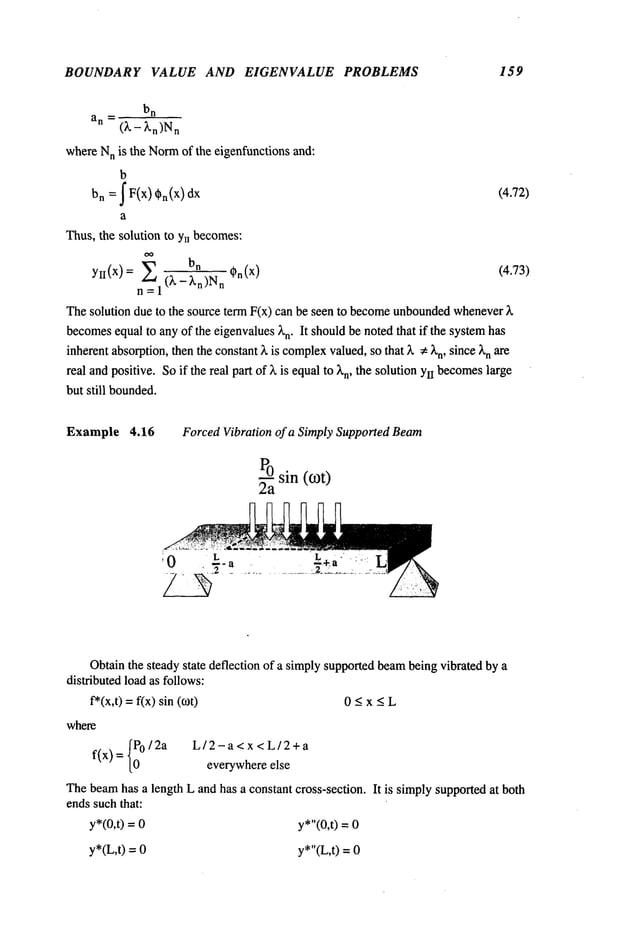
![BOUNDARY VALUE AND EIGENVALUE PROBLEMS 161
L/2 *a. . sin(n~)sin(n~
]38= f f-- ~--Q-° ) sin (-~- x) dx = -
~ ~ ~a; ~ EI(n~a ~)
L/2-a
Thus, ~e ~lufion ~omes:
~
. .~. . .n~ .
~ __ s~n (7) sm (~a)
. ~_~=_ ~rO ~ 2 L
sin(~x)
If a ~ O, ~e ~s~but~ forcing function ~omesa concen~at~ force, P~, ~en ~e l~it
~f ~e sNufion approaches:
~- 2p 0 ~ sin(~) sin(~x)
For concen~ ~int so~ces ~d fomes, one c~ rep~nt ~em by D~ del~
functions (ap~ndix D). ~us, one ~n ~ep~esent f(x)
~e cons~nt bn c~ now ~ found using ~e sifting pm~yof Di~ac del~ funcfi~s
(~.4):
L
bn = -Po / ~(x- L / 2)sin (~ x)~ = -Po ~
)
0
4.18 Fourier Sine Series
Consider the following S-L system:
y"+ ~,y = 0 O<x<L
y(O) = y(L) =
In this case p = r = 1 and q = O. Theeigenfunctionsand eigenvaluesof the systemare:
¯ nK
q~n(X)
=s~n(--~-- n =1, 2, 3
n2~
2
~Ln-- L
2
the orthogonality integral becomes:
L
sin(-~-x)sin(~-~x) n ~: m
.0
and the Normbecomes: ..](https://image.slidesharecdn.com/advancedmathematicalmethodsinscienceandengineering-hayek-230318001731-2b30ece5/85/advanced-mathematical-methods-in-science-and-engineering-hayek-pdf-175-638.jpg)
![CHAPTER 4 162
F(x)
Fig. 4.17
2L
L
N sin( x) = sin(n=x) dx--- n=1,2,~ ....
¯ ~ L )
0
Afunction F(x) can be expanded
into an infinite Fourier sine series as follows:
, ~[F(x+)+F(x-)]= Eansin(--~x)
O<x<L
n=l
wherethe Fourier coefficients an ~e given by:
L
an = ~ f F(x) sin n~ x (4.74)
L~ L
0
Thefunction F(x) is represented by ~e seres at ~l points in the region 0 < x <
~e seres represents an oddfunction in the region -L < x < L, since:
sin (- ~ x)= - sin (~
~us, the series also represents -F(-x)in the region -L < x < 0. Theseres also represents
a periodic function in the openregion -~ < x < ~ with periodicity = 2L, since:
sin(~ (x ~ 2~)) = sin~ n~ :) cos(2nm~) ¯ cos(~ x) sin
= sin (~ x) for all integers m
Thus,the Fourier sine series represents a periodic function eve~ 2L, with ~e function
being oddwithin each region of periodicity = 2Las shownin Fig 4.17.
At the two end points x = 0 and x = L, each te~ of the series vanishes, eventhough
the function it represents maynot vanish at either poim.Thisis due to ~e fact that since
¯ e series represents an oddfunction in the periodic regions = 2L,there will be an ordinal.](https://image.slidesharecdn.com/advancedmathematicalmethodsinscienceandengineering-hayek-230318001731-2b30ece5/85/advanced-mathematical-methods-in-science-and-engineering-hayek-pdf-176-638.jpg)
![BOUNDARY VALUE AND EIGENVALUE PROBLEMS 163
discontinuityat x =0, +L, +2L..... suchthat the function averagesto zero at the end
points(see 4.74), i.e.:
Example 4.17
Expand
the followingfunction in a Fourier sine series.
f(x): L-X 0-< x < L
2
L
_~2 f(L_X
] = 2L II_ <-l)n
1
an- L.I 2) sin mz xdx
L n~[_ 2 J
0
f(x)- 2.__~_L~t
2 n sin(-~
n=l
If onesets L= 1 andx = 1/2:
,~ I1- (-1)n
3 2 2/ 2 _ . on 3 "~ lsin(~)
~’=~" n s~n(-~-)=~- 2
n=l n =1,3,5
-==i-!+!-!+...
4 3 5 7
or
Thelast series canbe usedto calculatethe series for
n=1,2,3 ....
4.19 Fourier Cosine Series
TheFourier cosine series can be developed
in a similar mannerto the Fourier sine
series.
Consider the following S-L system:
y"+~y = 0 0<x<L
y’ (0) = y’ (L)=
In this case, p =r =1 andq = 0.
Theeigenfunctions and eigenvalues of the systembecome:
,~.(x)=cos
(--~- n=O,1, 2](https://image.slidesharecdn.com/advancedmathematicalmethodsinscienceandengineering-hayek-230318001731-2b30ece5/85/advanced-mathematical-methods-in-science-and-engineering-hayek-pdf-177-638.jpg)
![CHAPTER 4 164
n2~
2
~’n-- L
9
with the orthogonalityintegral definedby:
L
fcos (n~x) cos (x) dx = 0 n
L L
0
and the normgiven by:
L 2
N(cos (~ x)) : f(cos(nn x)] L
~ L J e
n
0
wheree, is Neumann’s
Factor, e0 = 1 and e, = 2, n ~ 1.
Afunction F(x) can be expanded
into an infinite Fourier cosine seres as follows:
n=O
wherethe Fourier coefficients bn are givenby:
L
_ En
bn - ~IF(x)cos(~x) (4.75)
0
Thefunction F(x) is representedby the seres at all points in the region0 < x <
Theseries represents an evenfunction in the region-L < x < L, since:
cos/_
x
):codex)
Thus,the series represents F(-x) in the region-L < x < 0. Theseries also represents
periodic function in the openregion -~ < x < oo, witha periodicity =2L, since:
cos(-~ (x+ 2mL)/=cos (-~ x)cos (2nm~t)T-sin (-~ x)sin
= cos (-~ x) for all integer valuesof m
Thusthe Fourier cosine series represents a periodic f~nctionevery 2L, with the function
being evenin the periodic regions = 2Las shown
in Fig. 4.18:](https://image.slidesharecdn.com/advancedmathematicalmethodsinscienceandengineering-hayek-230318001731-2b30ece5/85/advanced-mathematical-methods-in-science-and-engineering-hayek-pdf-178-638.jpg)
![BOUNDARY VALUE AND EIGENVALUE PROBLEMS 165
F(x)
-3L -2L -L L 2L 3L
x
Fig. 4.18
Sincethe series represents an evenfunction, then the series doesrepresent the
function F(x) at the end points x = 0 and x =
Example 4.18
Expand
the followingfunction in a Fourier cosine series:
f(x) = L x
2
bn = En ~(L- ~) cos(-~x) = [- 34 L
Thus
f(x)= 3L+4 2~L~ ~ ~cos(~x)
n=1,3,5
O<x<L
n=O
n>l
4.2 0 Complete Fourier Series
Since the Fourier sine andcosine series represent an oddandan evenfunction
respectively in the region -L < x < L, then it can be shown
that an asymmetricfunction
F(x) can be expanded
in both series in the region -L < x < L. Let F(x) be a function
definedin -L <x < L, then:
Denoting:
½IF(x)
+F(-x)]
Fl(x)
F(x)=½IF(x)-
F(-x)]](https://image.slidesharecdn.com/advancedmathematicalmethodsinscienceandengineering-hayek-230318001731-2b30ece5/85/advanced-mathematical-methods-in-science-and-engineering-hayek-pdf-179-638.jpg)
![CHAPTER 4 166
then Ft(x) and F2(x)represent evenand oddfunctions, respectively, since:
Fl(-x)=Fl(x) ana F:(x)=-
Hence,Ft and Fzcan be representedby a Fourier cosine and sine series, respectively:
V,(x):
Ebncos<-
n=O
where
L L
0 -L
F2(x) = Eaa sin(--~x)
n=l
where
L
-L<x<L
L L
1 ~F(x)sin(~x)dx
1 ~[Fl(X) + F:(x>]sin (~x) dx
an --~-
-L -L
¯ In these integrals, use wasmade
of the fact that:
L L
~Fl(X)sin(--~x) dx and ~Fa(x)cos(--~x) dx
-L -L
dueto the fact that the integrandsare oddfunctions.
Finally, the function F(x) canbe represented by the completeFourier series
follows:
where
Ean sin(--~x) + Ebn cos(~x)
n=l n=O
L
2 fF2(x)sin(_.~x)d x:_~1 F2(x)sin(.~.x)dxt.
an =~ L
0 -L
Thus,onecan rewrite the integrals for the Fourier coefficients as:
+L L
= e--m ~F(x)cos(~x)dx
-L -L](https://image.slidesharecdn.com/advancedmathematicalmethodsinscienceandengineering-hayek-230318001731-2b30ece5/85/advanced-mathematical-methods-in-science-and-engineering-hayek-pdf-180-638.jpg)
![BOUNDARY VALUE AND EIGENVALUE PROBLEMS 167
L
1fF(x)si.(nx)
an=’~ .~ L
-L
L
"% ~F(x)cos(~x)
bn =’~
-L
Notethat the eigenfunctionsare completelyorthogonalin (-L, L) since:
L
~ sin(nn x) sin (..~ x) dx = {0
L L n=m
-L
(4.76)
L
~ cos(__~ x) cos(_~ x) dx = f0
2Lien n=m
-L
+L
f. n~
m~ ,
sin- x cos-- x ax = 0 for all n, m
L L
-L
Onecan developthe completeFourier series representation from the S-Lsystem. Let
a S-L systemgiven by:
y"+ ky = 0 -L < x < +L
y(-L) : y(L)
y’(-L) = y’(L)
Thesystemis a proper S-Lsystem, since the operator is self-adjoint and the boundary
conditions are those of the periodic type. Thesystemyields the followingset of
eigenfunctions and eigenvalues:
n2/~
2
Z,n -- -~--
Theentire set of eigenfunctions
is orthogonal
overI-L, L], as givenabove.
In a more
generalform,the complete
Fourierseries, orthogonal
overa range[a, b]
canbe stated as follows:
-- ,,°° o:_(2nn(x-a))~ n (, 2n~- a)
F(x)~ ~an ~’"/" + cos a<_x<_b
n=l n=0](https://image.slidesharecdn.com/advancedmathematicalmethodsinscienceandengineering-hayek-230318001731-2b30ece5/85/advanced-mathematical-methods-in-science-and-engineering-hayek-pdf-181-638.jpg)
![CHAPTER 4 168
whereT = b - a, and the Fourier coefficients are givenby:
b
an = -~f F(x)sin(-~(x - a))
a
b
bn : ?I F(x) cos(-~ (x - a)/dx
a
(4.77)
Example 4.19
Obtainthe expansionof the followingfunction in a completeFourier series:
F(x) = {0L
x -L<x<0
-- 0<x<L
2 -
L
b0 = (L - ~-) dx =
0
L
bn= 1Ldr F(x)cos (n~ X)Ldx=2n~L~2
- (-1)
n]
0
n>l
L
an = ~ I F(x)sin (-~ x) dx :
0
n>l
3L L ~ 1 .n~
,~ [1- ] n~
-if-+ rt "~" ~-~ ~-Tc°st--~--x)+Ln
z~ n sin(L x)
n =1,3,5 n=l
In general, the fact that the integrals of the type givenin (4.74 to 4.77) must
converge,requires that F(x) mustsatisfy the followingconditions overthe range [L, -L]:
(a) piecewise continuous
(b) havea first derivative that is piecewisecontinuous
(c) have a finite numberof maxima
and minima
(d) single valued
(e) bounded
Theconditions imposedon F(x) listed aboveare quite relaxed whencompared
with
those imposedon functions to be expanded
by Taylor’s series.
Thefollowing general remarkscan be madein regard to expansionsof F(x) in
Fourier sine, cosine, or completeseries:](https://image.slidesharecdn.com/advancedmathematicalmethodsinscienceandengineering-hayek-230318001731-2b30ece5/85/advanced-mathematical-methods-in-science-and-engineering-hayek-pdf-182-638.jpg)
![BOUNDARY VALUE AND EIGENVALUE PROBLEMS 169
(a) Theseries convergesto F(x) at every point whereF(x) is continuous
(b) Theseries convergesto [F(x
÷) + F(x-)]/2 at a point of ordinarydiscontinuity,
i.e., wherever
F(x) is discontinuous
but has finite right andleft derivatives.
(c) Theseries represents a periodic function in the openregion -~ < x <
(d). Theseries convergesuniformlyand absolutely in -L < x < L if F(x)
continuous, F’(x) is piecewise continuousand F(L) = F(-L).
(e) Theseries can be differentiated termby termif F(x) satisfies the conditions
(d),i.e.:
F’(x)~~ ~ n(a n n~ , . n~x)
cos--L- x - on sin ~
n--1
(f) If F(x) is piecewisecontinuousthen one mayintegrate the series term by term
any number
of times, i.e.:
7t ~ n cos L x+--~t
sin x+box
n=l n=l
Thisseries converges
faster than the series for F(x).
4.21 Fourier-Bessel Series
Considerthe following system:
x2y"+xy
’+(t22x2-a2)y=0 0_<x_<L
with y satisfying the followingconditions:
y(0) is bounded VlY(L)+"~ 2Y’(L)
where~q, Y2are known
constants.
Thesystemis first transformedto S-Lsystem, havingthe form:
d----(xdY)+(t~2x-~-/dx
y=0
where
p(x) = q(x) = -a2/x r(x) =
The solution to the differential equationbecomes:
y = C1Ja(Ctx
) + C2Ya
(CtX)
Sincep(0) =0, then y(0) mustbe finite and py’ ---> 0. This requires that 2 m
ust be set
to zero to insure that y(0) is bounded.Thus,the remainingsolution:
y = C1Ja((~x
)
satisfies the conditionthat:](https://image.slidesharecdn.com/advancedmathematicalmethodsinscienceandengineering-hayek-230318001731-2b30ece5/85/advanced-mathematical-methods-in-science-and-engineering-hayek-pdf-183-638.jpg)
![CHAPTER 4 1 70
Lim xJ~(ax)~
x---~0
Theboundarycondition at x = L takes the followingform:
~(~) =0
’~lJa (C~x)+
°x x = L
resulting in the followingcharacteristic equation:
=
(4.78)
or
L2
{
Nn=2"~n2kt2n-a2+’~2 jJa2(l’tn)
Thecharacteristic equationcan be transformed(see 3.14) to the followingform:
(~’1 +~’~)Ja(ltL)-~-~ Ja+l(ILl’) = (4.79)
a transcendentalequation with an infinite number
of roots
If a * 0, then the first root is gt0=0 but it is not an eigenvalue,sinceCa(0)-- 0. If
a = 0, then there is a root I%=
0 onlyif’h= 0, otherwisegt0=0 is not a root in generalif
a = 0. Theeigenfunctions and eigenvalues become:
X. = ~2n
L
(a) Fora~O
Cn(x) = Ja(P,n n=1,2 .... (4.80)
(b) For a = 0 and YI= 0
c.(X) = J0/~n n=0,1,2 .... (4.81)
(c) For a= 0 andyt ¢
¢.(x) = Jo(~. n=1,2,3 .... (4.82)
Thenormof the eigenfunctions can be computed
from (3.109) as follows:
L
2 X
Nn= N(~Pn)= fXJa( tLn "~/dx2brat " L2 D2 ~l.n[Ja(~n)] } (4.83)
=.~.~j.Ln_a2)j2a(~tn) + 2 ,
2
0
Substituting in turn for J~(ktn) and Ja(ktn) in (4.81)oneobtains:
L2{( 2 a2, y~ }[
Nn = ~ ~n - ] ~,12----~ + 1 J~a(~n)]
(4.84)](https://image.slidesharecdn.com/advancedmathematicalmethodsinscienceandengineering-hayek-230318001731-2b30ece5/85/advanced-mathematical-methods-in-science-and-engineering-hayek-pdf-184-638.jpg)
![BOUNDARY VALUE AND EIGENVALUE PROBLEMS 171
Thus, if y, = 0, hence J~(~t,)= 0, then the normbecomes:
Nn = gn -a2 Ja~(~tn) n > 1 (4.85)
and if’~z = 0, hence Ja(gn) = 0, then the normbecomes:
L2 , 2
N
n = T [Ja(~n)] n >_ 1 (4.86)
Expansion
of a function F(x), defined overthe range 0 < x < L, into an infinite series
of the Fourier-Bessel orthogonal functions Ja(p,, x]L) can be madeas follows:
F(x): Z bnJa(..~)
n = 0orl
where
L
hn = "~n I x F(x) Ja(btn ~-)
0
(4.87)
Example 4.20
Obtain an expansionof the following function:
F(x)= 0 < x < L
in a Fourier-Besselseries:
x
Cn(X) = Jo(I.t n -~) where Jo(IXn)
TheFourier coefficients are givenby:
L
bn=~-n XJo ~tn
dx= 2
0
~tn Jl(~tn)
and bo = 0, whereeqs. (3.14), (3.103) and (4.86) were
Thus,the Fourier-Besselseries representationof F(x) = 1 is:
1=2 Z Jo(gn X//L)
n = 1 ~l’nJl(~l’n)
n=1,2,3 ....
4.22 Fourier-Legendre Series
Considerthe followingdifferential equation:
(1- x2) y"-2xy’ + V(V+ 1) y = 0 -l<x<+l
wherey(1) and y(-1) are bounded.
Theequation can be transformedto an S-Lsystemas follows:](https://image.slidesharecdn.com/advancedmathematicalmethodsinscienceandengineering-hayek-230318001731-2b30ece5/85/advanced-mathematical-methods-in-science-and-engineering-hayek-pdf-185-638.jpg)
![BOUNDARY VALUE AND EIGENVALUE PROBLEMS 173
1
2n+l[
2n+l . .
an = ~J Pn(x) dx = ~ Pn_l(0) n>_1
0
1
2
where
the integral in (3.162)wasused,
1
an =~" n--0
=0
Thus:
= 2n+
2n(n+1) [(n- 1~),]
2
n = even,> 2
n= odd
f(x) = ½+ ¼Pl(x)- ~6P3(x)
1 3 7
ao 2 a~ ~- a2 = 0 a3 16](https://image.slidesharecdn.com/advancedmathematicalmethodsinscienceandengineering-hayek-230318001731-2b30ece5/85/advanced-mathematical-methods-in-science-and-engineering-hayek-pdf-187-638.jpg)
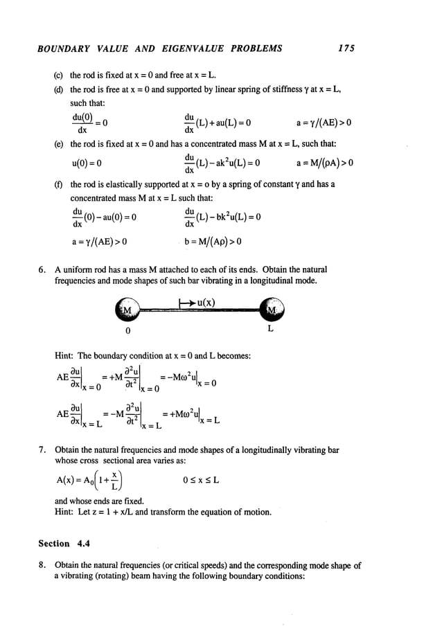
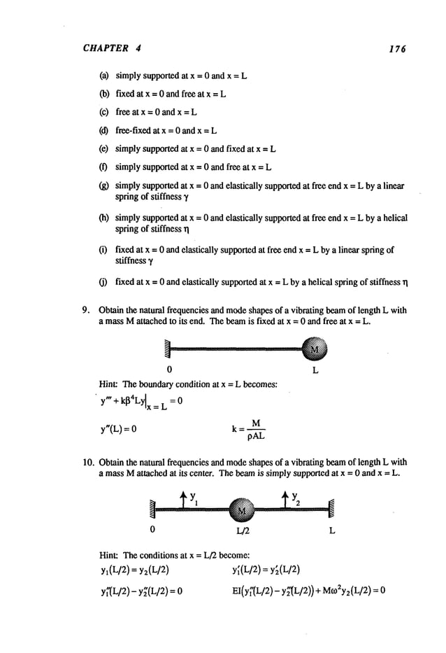
![BOUNDARY VALUE AND EIGENVALUE PROBLEMS 179
d4Y p d2y
EI d--~- +d--~- + ky =0 0<x_<L
wherep~ > 4k EI. Thecolumnis simply supported at both ends.
Section 4.11
19. Show
that the differential operatorsgivenin eq. (4.34) are self-adjoint.
20. Obtainthe conditionsthat the coefficients of a linear fourth order differential operator
mustsatisfy so that the operator canbe transformed
to a self-adjoint operator.
Section 4.15
21. Transform
the followingdifferential operators to the self-adjoint Sturm-Liouville
formgivenin eq. (4.49):
"/1- x~)" y" - 2xy’+~.y =
(a)
(b) (1-x~)y
"-xy ’+~,y:O
(C) (1- X2)2y"+ [~(1- X2)+ 1]
(d) xy"+(a+ l-x) y’+~.y
(e) y"-2xy’+Xy =
(f) (1- x2) y"- (2a + 1) xy’ +
(g) (1-x2)y"-[b-a-(a+b+2)x]y
’+~, y=O
(h) x(1- x) y"- [c- (a + b + 1) x] y’+ ~,y
(i) x2y"+xy’+(~,x2-2)y=O
x2y"+xy’+(~,xZ-n2)y:O
(k) (ax + b) y" + 2ay’+ ~.(ax + b)
(1) y" + 2a cotanax +~,y = 0
(m)
xy"+23- y’ +~,y=
0
(n) y"+ay’+~,y =
(o) y" - 2a tan axy’ + ~,y =](https://image.slidesharecdn.com/advancedmathematicalmethodsinscienceandengineering-hayek-230318001731-2b30ece5/85/advanced-mathematical-methods-in-science-and-engineering-hayek-pdf-193-638.jpg)
![CHAPTER
(u)
(w)
4
y" + 2a tanh axy’+ ky = 0
y"- a tan axy’+ ~, cos
~ axy =0
y" + 2axy’ + a~x2y+ ~,y = 0
y,,_ a~y,+ ~-4~y = 0
x~’y"- a(a- 1) x~-~y + ~,y =
x4y
" + ~y = 0
xy"+~.y = 0
xy" + 4y’ + ~xy = 0
y"+4y’+(~,+4) y =
- 2xy’ + ~ ~,x3y=
x2y
" 0
x2y"- xy’+ (~,+ 1) y =
xy" + 2y’ + Lxy= 0
x2y
" + 3xy’ + [kxs - 3] y = 0
xy" + 3y"+ ~,x-l/3y = 0
xy"+ 6y’+ ~,xy = 0
xy" + 4y’ + ~,x3y= 0
xy" + 2y’ + ~x3y= 0
x2y"+-~ xy" + ~(~,x3 - ¼) y =
a<O
integral for the followingdifferential systems:
(a) Problem 21a 0 <x _<1 y(O)= y(1)finite
(b) Problem 21a 0 <x _<1 y’(O) = y(1)finite
(c) Problem 21b -1 < x < 1 y~l) finite
180
(hh) xy"+~-y +kx3y=O
22. Obtainthe eigenfunctions Cn(x), eigenvalues L~and write down
the orthogonality](https://image.slidesharecdn.com/advancedmathematicalmethodsinscienceandengineering-hayek-230318001731-2b30ece5/85/advanced-mathematical-methods-in-science-and-engineering-hayek-pdf-194-638.jpg)
![CHAPTER 4
Section 4.17
23. Oblain the solution to the following systems:
(a) y"+ ~,y = f(x) y(L) =
(b) y"+-I y’+~y = y(L) =
x
(0) (1- X
2) y"-- 2xy’ + ~,y : f(x)
(d) y"- 2y’+ (l+l]) y x y(O)=
O<x<l
(e) xy"+(--32-x/y’+(x’3+ ~.~ ~
4 4 )Y=
O_<x<l
(f) xyO+(3-2x) y’+ (a2x3 + x- 3) x
182
O<x<l
(g) xy" + 2y’ + k2xy= 1 y(1) =
(h) xy" +(3- 2x)y’ +(~.x 2- 3x))y= e-- ~-x
x
O<x<l
(i) x2y "+[3-6x]xy’+[9x~-9x-15+~,x’]y= x~e
sx
O<x<l y(1)=O
y(O)=
y(O)finite
y(+l) finite
y(1) =
I~ is a fixed constant
y(O)finite (bounded)
yO)=0
y(O)finite
y(1) =
y(O)finite
y(O)finite (bounded)
y(1) =
y(O)finite (bounded)
(j) x2y"+ 2(1-2x)xy’+(~.x 4 +4x2 -4x-~)y=x~e
2x
0 < x < 1 y(1) = y(O)finite (bounded)
x2y,, + (_52 _ 2xl xy, + (kx4 + 2-’~5x -i- ~)y=7~eX
x
~
0 < x < 1 y(1) = y(O)finite (bounded)
(1) x2y"+2(l+x)xy’+(Lx 4 +x2+2x)y=e-Xx
3
0 _<x < L y(L) = y(O) finite Coounded)
(m) xy" +(4-2x) y" +(Z.x5 + x-n) y = x2e
x](https://image.slidesharecdn.com/advancedmathematicalmethodsinscienceandengineering-hayek-230318001731-2b30ece5/85/advanced-mathematical-methods-in-science-and-engineering-hayek-pdf-196-638.jpg)
![FUNCTIONS OF A COMPLEX VARIABLE 18 7
Imaginary Axis
Y .
y Zo(Xo,yO
~ RealAxis
X
Fig,. 5.1. Vector Representation of the Complex Plane
tan 0 = Yo, 0 < 0 _<2r~ or -n <0 <r~
x
o
and the angle 0 is called the Argument
of Zo.
Thecomplexnumber
Zodoes not changevalue if 0 is increased or decreasedby an
integer number
of 2rt, i.e.:
zo =rei° =re
i(0-+2n~) n = 1, 2, 3
Thus,in the polar form,let a = rlei°~, b = r2ei°2 then their productis:
ab = rlraei(°l+%)= rlr2[cos(01 + 02)+ isin(0~ +02)]
and their quotient is givenby:
a = r~ei(O,-02): rl [cos(0~ _02)+ isin(0,-02)
]
b r
2 r
2
In polarrepresentationthe expression[z - zol =c representsa circle’centeredat zo and
whoseradius is "c".
5.1.3 Absolute Value
Theabsolute valueof zo represents the distance of point zo fromthe origin. Theabsolute
value of the difference betweentwocomplexnumbers,is:
la- bl =~/(a, - b~)2+ (a2 - 2
and represents the distance between
a and b.
Theabsolute value of the products and quotients become:
labcl =](https://image.slidesharecdn.com/advancedmathematicalmethodsinscienceandengineering-hayek-230318001731-2b30ece5/85/advanced-mathematical-methods-in-science-and-engineering-hayek-pdf-201-638.jpg)
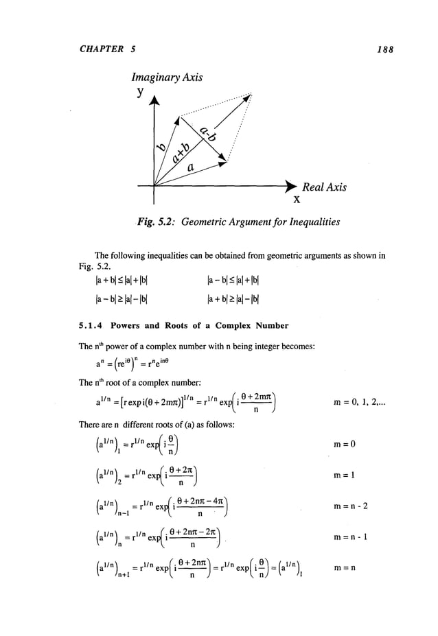
![FUNCTIONS OF A COMPLEX VARIABLE 189
a-E a
(a)
Fig. 5.3
Imaginary Axis
y ~,
(b)
~-- ReaI Axis
X
Succeeding
roots repeat the first n roots. Hence,a1/n has n distinct roots. In polar form,
the n roots fall on a circle whose
radius is r1/n and whosearguments
are equally spacedby
2n/n.
5.2 Analytic Functions
Onemustdevelopthe calculus of complex
variables in a treatment that parallels the
calculus of real variables. Thus,one mustdefine a neighborhood
of a point, regions,
functions, limits, continuity, derivatives and integrals. In each case, the corresponding
treatmentof real variables will be presentedto give a clearer picture of the ideas being
presented.
5.2.1 Neighborhood of a Point
In real variables, the neighborhood
of a point x = a represents all the points inside
the segmentof the real axis a - e < x < a + e, with e >0, as shown
in the shadedsection
in Fig. 5.3a. This can be written in morecompactformas ~ - a I< e.
In complex
variables, all the points inside a circle of radius e centeredat z =a, but not
includingpoints on the circle, make
up the neighborhood
of z = a, i.e.:
]z - a[<e
This is shown
as the shadedarea in Figure 5.3b.
5.2.2 Region
Aclosed regionin real variables contains all interior ~as well as boundarypoints,
e.g., the closedregion:
Ix-l[_<X
contains all points 0 < x < 2, see Fig. 5.4a. Theclosed region in the complex
plane
contains all interior points as well as the boundary
points, e.g., the closedregion:](https://image.slidesharecdn.com/advancedmathematicalmethodsinscienceandengineering-hayek-230318001731-2b30ece5/85/advanced-mathematical-methods-in-science-and-engineering-hayek-pdf-203-638.jpg)
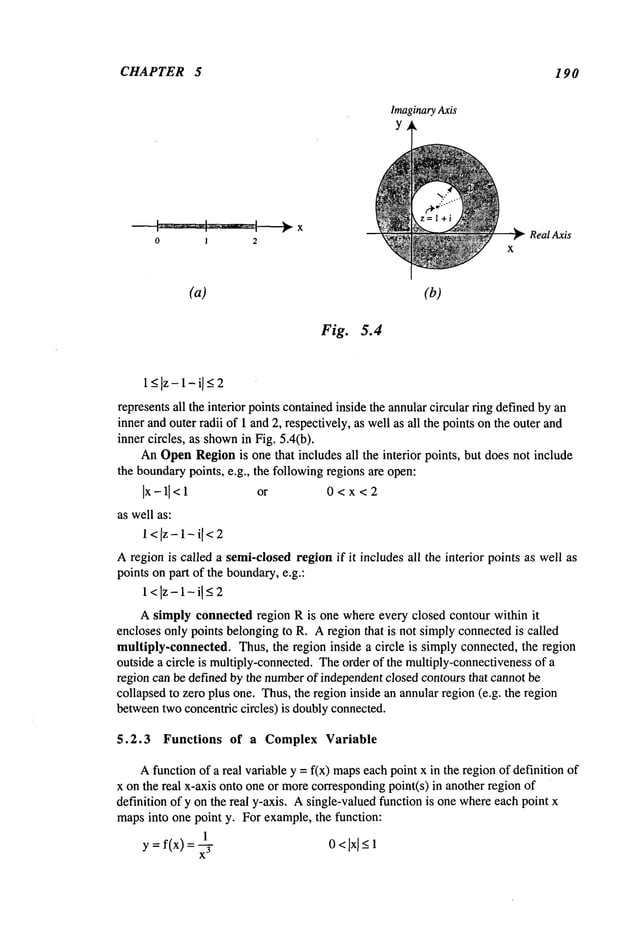
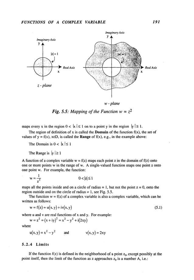
![CHAPTER 5 192
Lim f(z) = (5.2)
z~z
0
This meansthat if there exists a positive small number
~ such that:
[z - z0[<e then Iw-A
I <~for a small positive number~
Thelimit of the function is unique.
Let Aand Bbe the limits of f(z) andg(z) respectively as z 0,then
:
LimIf(z) + g(z)] = A
z--~z
0
Lim[f(z) g(z)]
z~z
0
Lim f(z) A providedthat B~ 0
z -~ z0 g(z)
Sincethe limit is unique, then the limit of a function as z approachesz0 by any path C
mustbe unique. If a function possesses morethan one limit as z --~ z0, whenthe limiting
processis performed
alongdifferent paths, then the function has no limit as z --~ z0.
Example 5.1
Find the limit of the followingfunction as z --~ 0:
xy
2
fl(z) = 2 +y4
Let y = mxbe the path Calongwhicha limit of the function f~(z) as z --~ 0 is to
obtained:
m2x
3
Lim f~(z)= Lim ~0
z-~0 x ---~ 0 +m2x4
independentof the value of m. This is not conclusive because, on the curve x = my
2, the
limit of f(z) as z ~ 0 on Cis m/(m
2 + 1), whichdependson mfor its limit. Thus, if
f~(z) has many
limits, then f~(z) has nolimit as z --~
5.2.5 Continuity
Afunction is continuousat a point z = z0, if f(Zo) exists, and Limf(z) exists,
z-~z
0
if Limf(z) = f(zo). A complexfunction f(z) is continuous at z = Zoiff, both
z~z
0
andv(x,y) are continuousfunctions at z = o.](https://image.slidesharecdn.com/advancedmathematicalmethodsinscienceandengineering-hayek-230318001731-2b30ece5/85/advanced-mathematical-methods-in-science-and-engineering-hayek-pdf-206-638.jpg)
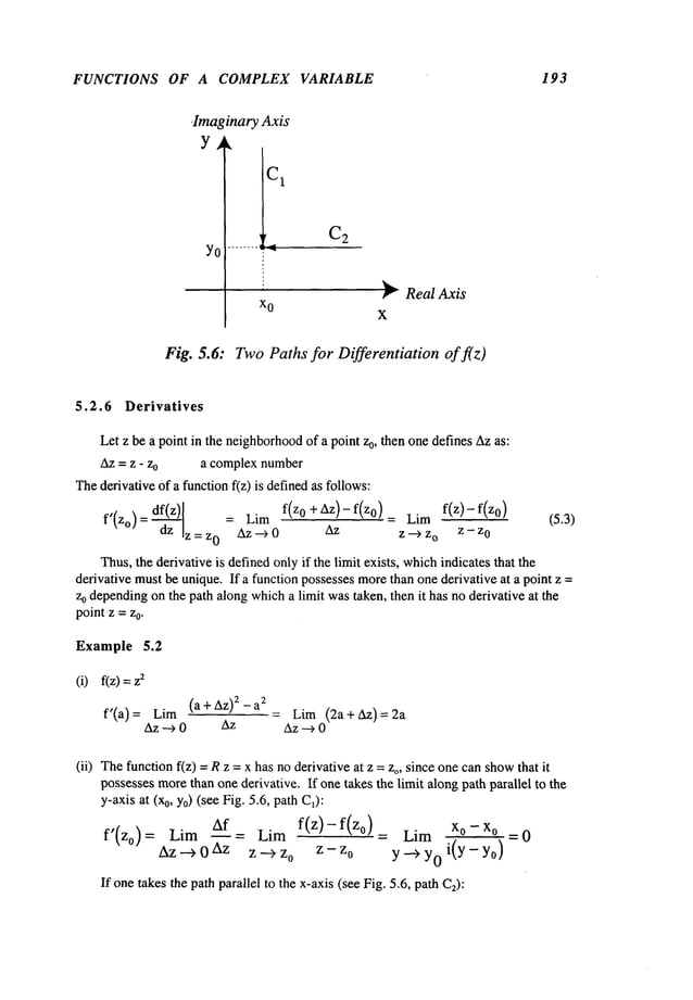
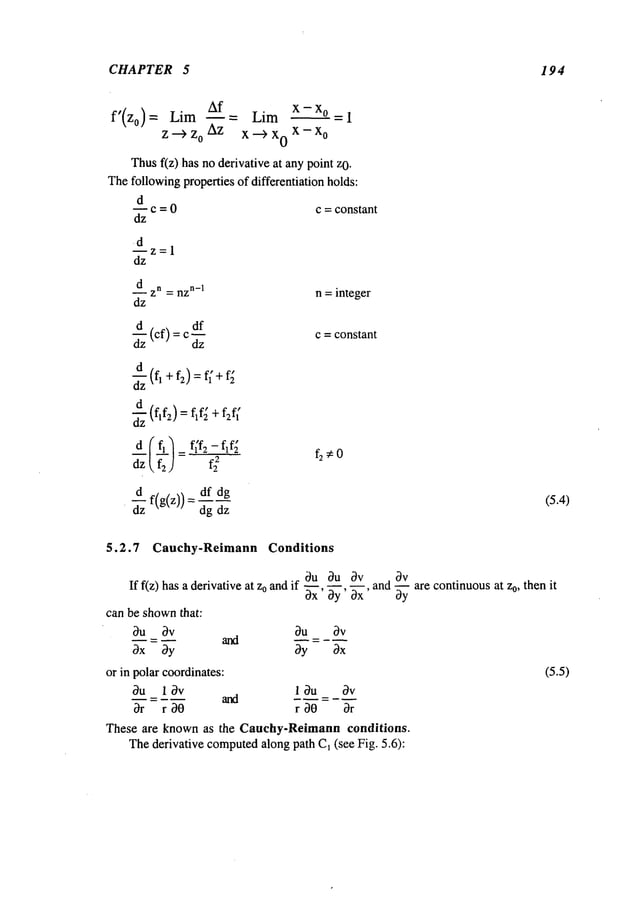
![FUNCTIONS OF A COMPLEX VARIABLE 195
f’(Zo) = Lim
z--)z
0
on C
1
f(z)-f(zo)
Z-- Z
0
= Lim
Y -~ YO (x° + iY)-(x° + iYo)
on C
1
[U(Xo,Y)+iV(Xo,Y)]- [U(Xo,Yo)+
iv(x0,
U(Xo,y)- U(xo,Yo)
= Lira
Y--> YO i(
y-yo
)
on C
1
¯ ~u ~v
= - 1-~y(x0, y0) +-~y (x0, 0)
Thederivative computedalong path C2becomes:
f(z)- f(zo)
f’(zo) = Lim
z ---> z
0
z - z
o
on C
2
Lim
Y--) YO
onC
1
= Lim
x--~x
0 (x + iyo)- (Xo+iYo)
on C
2
V(Xo,Y)- V(Xo,Yo)
Y- YO
[u(x, Yo)+iv(x, Yo)]- [U(Xo,YO)+
iv(xo,
u(x’ Y°)-u(x°’Y°)+i v(x, yo)- V(Xo,Yo)
= Lim Lim
x ---> x
0 x - x
o x --> x
0
x - x
o
on C
2 on C
2
Ou . Ov
= -~x (x0, y0)+1-~x(x0, )
Thus, equating the two expressions for f’(z), one obtains the Cauchy-Riemann
conditions given in eq. (5.5)¯ TheCauchy-Riemann
conditions can also be written in the
polar formgiven in (5.5)¯ Thederivative can thus be evaluated by:
f’(z)=Ou .3v
bu
~x + ~ - " (5.6)
0x 0y
1 ~y
Example 5.3
(i) Thefunction:
f(z) = 2 =(x2 - y2)+i(2xy)
u(x,y) = x2-y
2 v(x,y) = 2xy
has a derivative:](https://image.slidesharecdn.com/advancedmathematicalmethodsinscienceandengineering-hayek-230318001731-2b30ece5/85/advanced-mathematical-methods-in-science-and-engineering-hayek-pdf-209-638.jpg)
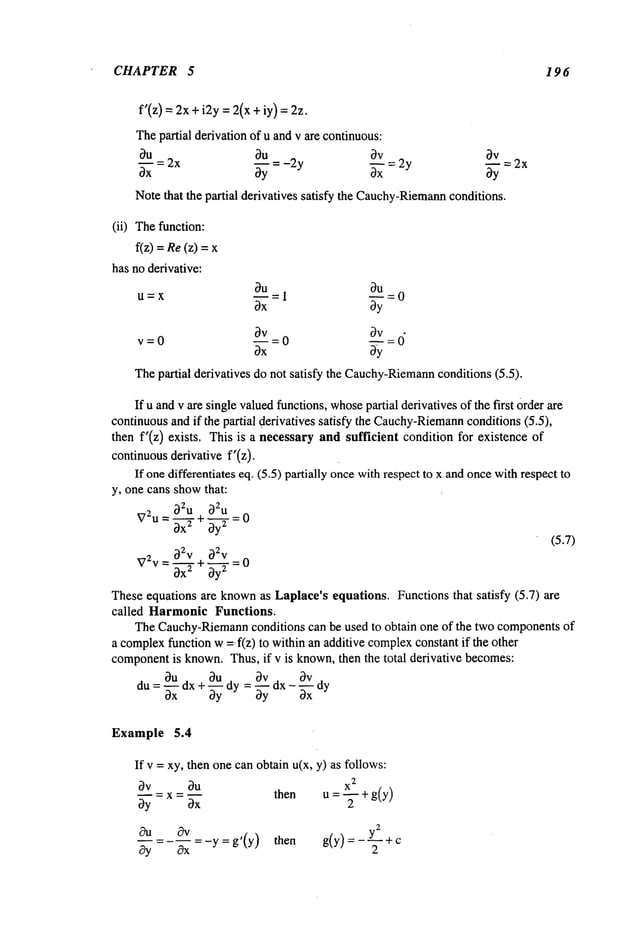
![FUNCTIONS OF A COMPLEX VARIABLE 19 7
Thus,the real part u(x, y) is givenby:
U =~(X2 -y2)+C
SOthat the functionf(z) is:
f(z) = ~(x2 - yZ)+c+ixy = ~ z2
5.2.8 Analytic Functions
Afunction f(z) is analytic at a point o if i ts derivative f’(z) e xists and i
continuousat Zoand at every point in the neighborhood
of zo. Anentire function is one
that is analytic at everypoint in the entire complex
z plane. If the function is analytic
everywhere
in the neighborhood
of a point zo but not a z = z0, then z =Zois called an
isolated singularity of f(z).
Example 5.5
(i) Thefunction:
f(z): °
(ii)
n=0, 1,2 ....
is an analytic function since f’(z) = n-~ exists an d is con
tinuous eve
rywhere. It is
also an entire function.
Thefunction:
1
f(z) = (z - 2
is analytic everywhere,
exceptat z0 =1, since f’(z) =- 2/(z - 3 do
es not exist at
zo =1. Thepoint z0 = 1 is an isolated singularity of the function f(z).
5.2.9 Multi-Valued Functions, Branch Cuts and Branch Points
Somecomplexfunctions can be multivalued in the complexz-plane and hence, are
not analytic over someregion. In order to makethese functions single-valued, one can
define the rangeof points z in the z-planein a waythat the functionis single-valuedfor
those points. For example,the function zl/2 is multivaluedsince:
w=z1/2= [l’ei(°:t2nn) ]1/2 =1"~/2i(°-+2nn)/2 r>0,0<0 < 27z
Therefore,for n =0:
zI/2 =r1/2 eiO/2
andfor n =1:
z1/2 = r1/2 ei(0+2n)/2](https://image.slidesharecdn.com/advancedmathematicalmethodsinscienceandengineering-hayek-230318001731-2b30ece5/85/advanced-mathematical-methods-in-science-and-engineering-hayek-pdf-211-638.jpg)
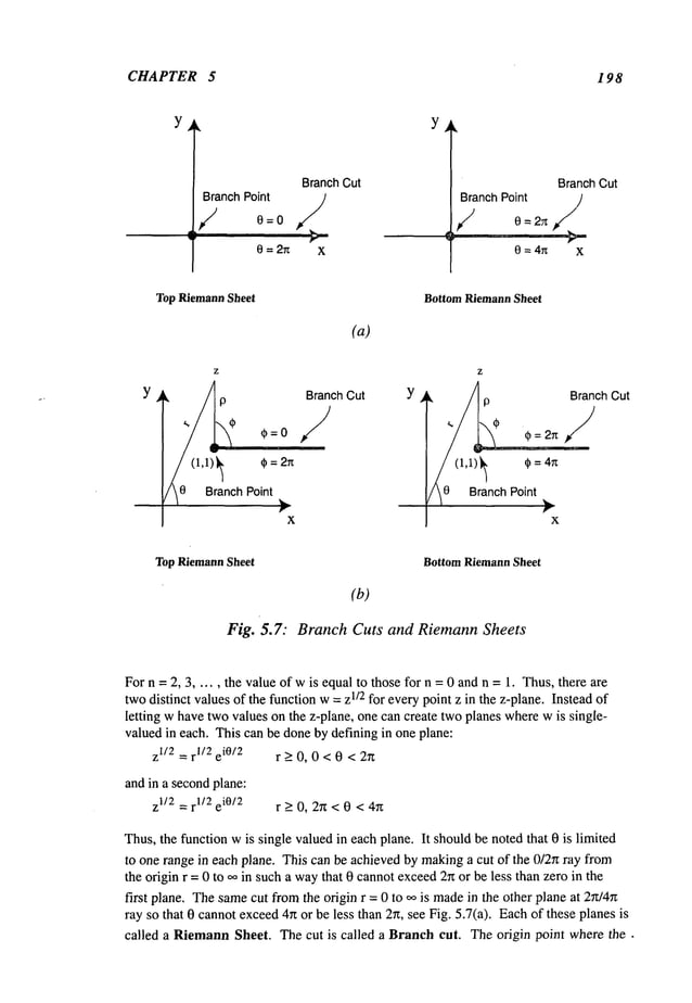
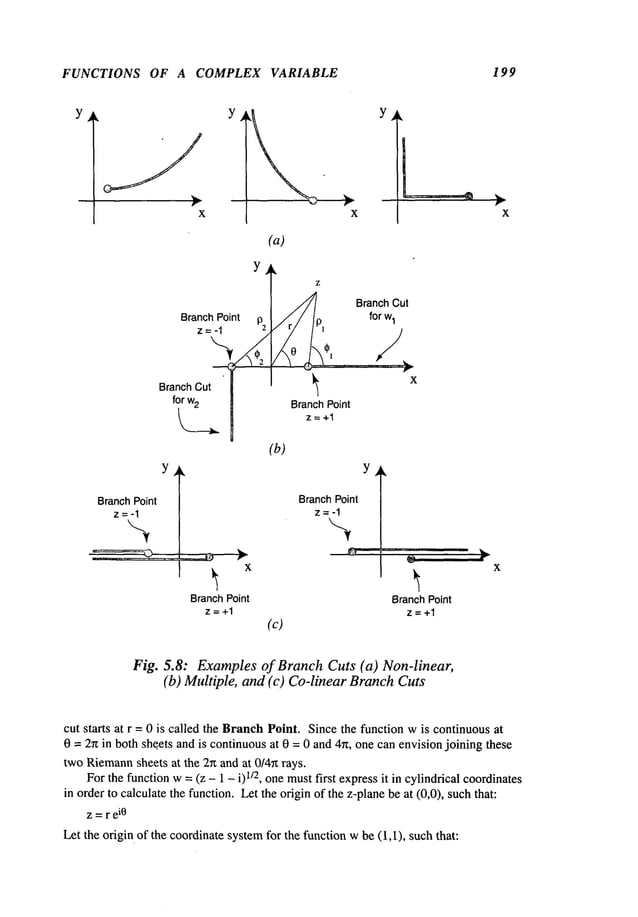
![FUNCTIONS OF A COMPLEX VARIABLE 205
where-~ < c~ < 0 then there is an infinite numberof Riemann
sheets. TheRiemann
sheet
with n = 0 is called the Principal Riemann
sheet of log z, i.e.:
logz= logr+i0 r > 0 ~ < 0 < ~ + 2n (5.19)
wherethe choiceof + 2~ is madein order to include the angle 0 = 0 in the Principal
Riemann
sheet. Thefunction log z as defined by (5.19) is thus single-valued. The
function log z is not continuousalong the rays defined by 0 = ~ and 0 = c~ + 2n, because
the function jumpsby a value equal to 2hi when0 crosses these rays. Since the function
is not single-valued on 0 = ~ and 0 = ~ _+2~, the logarithmic function has no derivative
on the branchcut defined bythe ray 0 =c~, as well as at the branchpoint z0 = 0. Hence,
all the points on the ray 0 = (~ are non-isolatedsingular points.
Afew other formulaefor the complexfunction are listed below:
(logz)
1 =- z~0 r>0 ~<0<~+2~
z
el°gz = el°gr+i0 = el°gre i0 = rei0 = z
logeZ= log(eX)Iei(Y+-’2nr~)l
=x +iy +2inrt =z +
log z~z
2 = logz~ +log z
2
logzl = logz1 - logz
2
Z2
log Zm = mlog z
5.3.6 Complex Exponents
Definethe function za, wherea is a real or complex
constant as:
za = eal°gz = e
a[l°gr+i(0:l:2n~)] ~ < 0 < ~ _+2~ (5.20a)
Theinverse function can also be definedas follows:
1
7~
-a
Z
a
Thefunction za is a multi-valuedfunction when
the constant "a" is not an integer, unless
one specifies a particular branch.
To achieve this, one can follow the samemethodof makingthe function single-
valued on each of manyRiemann
sheets.
Defining:
za = eal°gz = e
a[l°gr+i0] (x +_2nr~<0 <ct +2(n+ 1)~ (5.20b)
where,n = 0, 1, 2 ...... then the function za is single-valued in each Riemann
sheet,
numbered
n = 0 (principal), n = i, 2 .....
Forexample,let a = 1/3 andlet c~= 0, then:
z1/3=r1/3e
i0/3 where2n~< 0 < 2(n + 1)Tz](https://image.slidesharecdn.com/advancedmathematicalmethodsinscienceandengineering-hayek-230318001731-2b30ece5/85/advanced-mathematical-methods-in-science-and-engineering-hayek-pdf-219-638.jpg)
![CHAPTER 5 206
Therefore,for n =0, 0 < 0 < 27z, for n =1, 2r~ <0 < 4n, and for n = 2, 4~z< 0 < 6r~.
For n = 4, the value of Z113 is the sameas defined byn = 0. Thus,there are only three
Riemann
sheets n = 0, 1 and 2.
Thederivative of za can be evaluatedas follows:
dz a = dealogz = aealogz = az
a- I
dz dz z
Theexponential function with a base "a", where"a" is a complex
constant, can be defined
as follows:
az -_ ezloga
daz=--ed
z~o~ao
=(loga)e
z~°ga =aZloga (5.21)
dz dz
5.3.7
Definethe inverse function arcsin z:
w= arcsin z or
or
eiw = iz + 1%]~-z
2
wherex/i - z2 is a multi-valued function. Thus:
Similarly:
i. 1-iz i. i+z . ¯
arctan z = -~ log ~ = -~ log ~ = -i arctanh(iz)
Inverse Circular and Hyperbolic Functions
eiw _ e-iW
z = sin w=
2i
(5.22)
Since the definitions involvemultivaluedfunctions, all the inverse functions are also
multivaluedfunctions.
Theinverse hyperbolicfunctions can be defined as follows:
arcsinh z = loglz +z~-~+1 ] =-i arcsin(iz
)
(5.23)
1 , l+z
arctanh z = 7 ~og1-~ = -i arctan(iz)](https://image.slidesharecdn.com/advancedmathematicalmethodsinscienceandengineering-hayek-230318001731-2b30ece5/85/advanced-mathematical-methods-in-science-and-engineering-hayek-pdf-220-638.jpg)
![FUNCTIONS OF A COMPLEX VARIABLE 207
5.4 Integration in the ComplexPlane
Integration of real functions is a process of a limiting summation.
Thus,integration
in the Reimann
sense can be defined as:
b N
~f(x)dx = Lim ~f(xj)(Axj)
N----~oo.
a j=l
whereAxj= xj -x~.1 and x0 =a and xr~ = b, Nbeingthe number
of segments.
Integration of a real function f(x,y) alonga path Cdefined bythe followingequation:
y = g(x) on C
can be performedas follows:
x
b
ff(x,y) ds = ~f[x,g(x)],f(g’)e
C xa
Onecan performthe precedingintegration by a parametricsubstitution, i.e. if one
lets x = ~(t) andhencey = g(x)= g(~(t)) = ~l(t), where<tu correspo
nd to the limi
ts a
andb, then the integral is transformed
to:
t
b
f f(x,y)ds
=f[~(t),tl(t)]~/(~’)2 +( 2 dt
C t
a
Integration of a real functionf(x,y) on twovariables (area integrals) canbe performed
follows:
N M
~f(x,y)dxdy= Lim ~ ~ f(xi,Yj)(Axi)(Ayj)
N,M--~,~
A i=lj=l
whereAx
i = xi - xi_1 and Ayj= yj - Y j-1.
5.4.1 Green’s Theorem
Atheoremthat transformsan area integral to a line integral canbe stated as follows:
If twofunctions,f(x,y) andg(x,y), togetherwiththeir first partial derivatives
continuousin a region R, and on the curve Cthat encloses R, then (see Fig. 5.9).
!/~f - ~g/dx dy = f[g(x,y) dx + f(x,y)
(5.24)
-~x OyJ
C
wherethe closed contourintegration on Cis taken in the Positive (counter-clockwise)
sense.
Similarly, one can define an integration in the complex
plane on a path C(Fig. 5.10)
by:](https://image.slidesharecdn.com/advancedmathematicalmethodsinscienceandengineering-hayek-230318001731-2b30ece5/85/advanced-mathematical-methods-in-science-and-engineering-hayek-pdf-221-638.jpg)
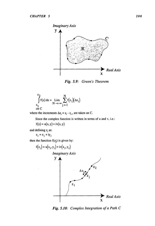
![FUNCTIONS OF A COMPLEX VARIABLE 209
with
Azj = Axj + iAyj
Theintegral can nowbe defined as a limit of a sum:
z2 N
~f(z)dz= Lim j~!u(x,,yj)+iv(xj,Yj)l[Axj+iAyj]
Zl
N-->~ =
~
"
xj,yj
on C
on C
N N
Lira E u(xj,yj) Axj - v(xj, yj) Ayj + i NLi.~m~j~l
u(xj, yj) Ayj + v(xj,yj) j
N-->~j=
1
.=
x2’ Y2 x2’ Y2
= ~ [u(x’y)dx-v(x,y)dYl+i ~ [u(x’y)dy+v(x’y)dxl
xl,Y
1 xl,Y
1
on C on C
Theintegration of a complex
function on path Cas defined in (5.25) has the
followingproperties:
b a
(i) ~ f(z)dz =-f f(z)
a b
on C on C
b b
(ii) J c f(z) dz = c j" f(z) dz c = constant
a a
on C on C
b b b
(iii) ~ [f(z)+ g(z)] dz= ~ f(z)dz + ~
a a a
on C on C on C
b c b
(iv) ~f(z) dz=~f(z)dz+~f(z)dz
a a c
on C on C on C
conC
on C
whereMis the maximum
value of If(z)lon Cin the range [a,b] and:
(5.25)
.26)](https://image.slidesharecdn.com/advancedmathematicalmethodsinscienceandengineering-hayek-230318001731-2b30ece5/85/advanced-mathematical-methods-in-science-and-engineering-hayek-pdf-223-638.jpg)
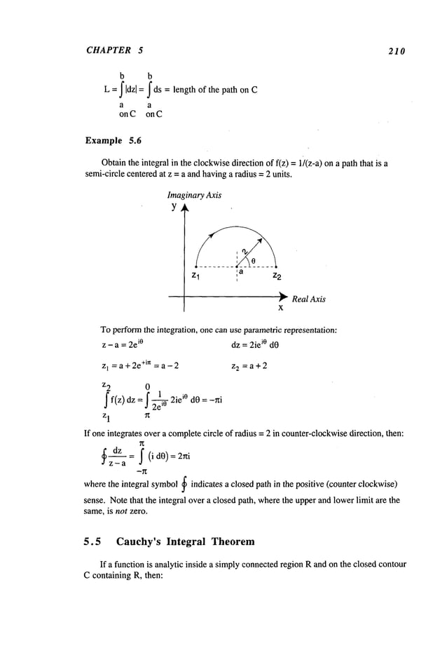
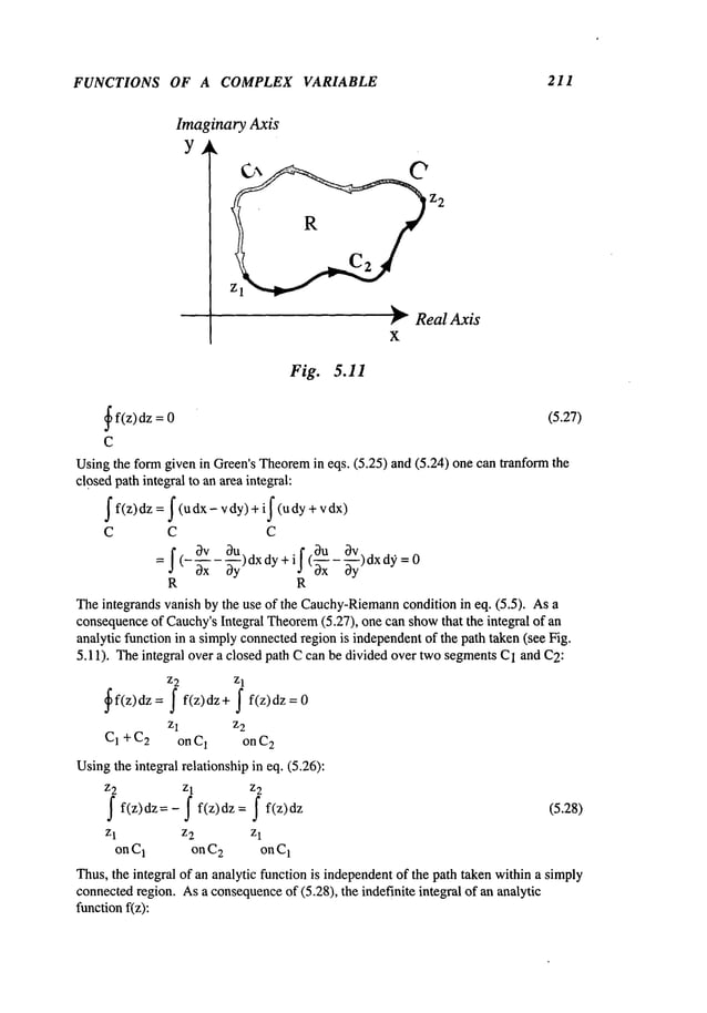
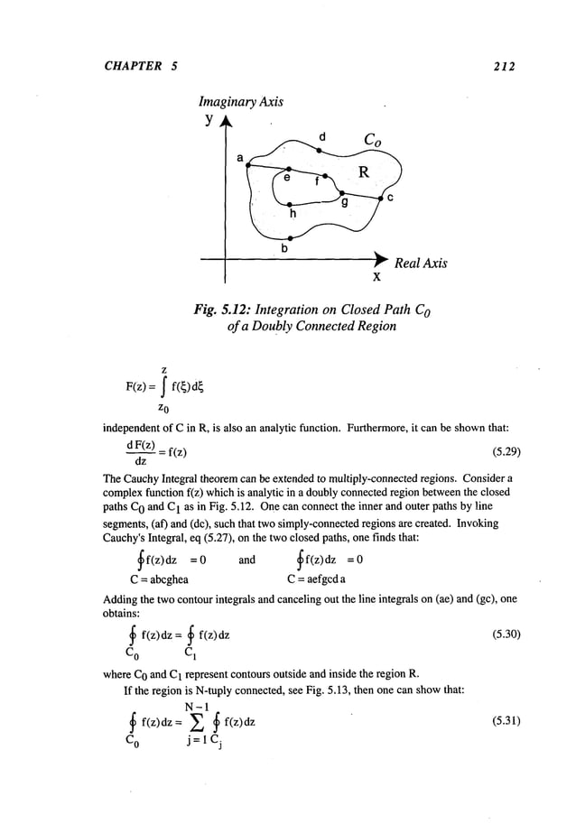
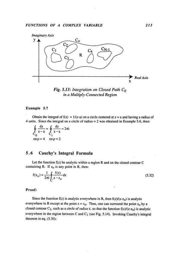
![CHAPTER 5 214
Imaginary Axis
Y
~: Real Axis
X
Fig. 5.14: Complex Integration over a Closed Circular Path
~dz=~ f(z) dz=~ f(z)-f(z°~dz+f(Zo)~
dz
Z-- Z--z
o
C C1 zo C1 z - z
o CI
= ~ f(z)-f(z°)dz+2nif(Zo)
Z-- Z
o
C~
by the use of results in Example
5.6.
Theremainderintegral mustbe evaluatedas e --> 0, usingthe results of (5.26):
Lim[~ f(z)-f(z°) dz]< Lim (If(z)-f(zo)ll2ue: Lim 2r~[f(z)-f(zo~-->0
e~0~l~ z-z
o
[- e~0 e 2 e--.0
[ onC
1 onC
1
since f(z) is continuousand analytic everywhereinside R. Cauchy’sintegral formulacan
be usedto obtain integral representation of a derivative of an analytic function. Usingthe
definition of f’(Zo) in eq. (5.3), andthe representationof f(Zo)in eq. (5.32):
f’(z°)=~z-~oLim
.f(z° + Az
)-az f(z°)’)
=~1 Lim__l ~I f(z) zf_(_~Zz)o z
2hi az~O~z Lz-<Zo
+ ~z)
= I.~ Lim ~
f(z) : dz--> 1 ~ f(z)
2~ri
az-~Oc
(z-Zo)(Z-
Zo- Az) 2~---~~
(Z-~o)2
Similarly,
itcan
beshown
that
the
n
thderivative
off(z)
can
berepresented
bythe
integral:
2n,n!! (z-’~o)
n+lf(z
f(n)(Zo)=_---r. dz (5.33)](https://image.slidesharecdn.com/advancedmathematicalmethodsinscienceandengineering-hayek-230318001731-2b30ece5/85/advanced-mathematical-methods-in-science-and-engineering-hayek-pdf-228-638.jpg)
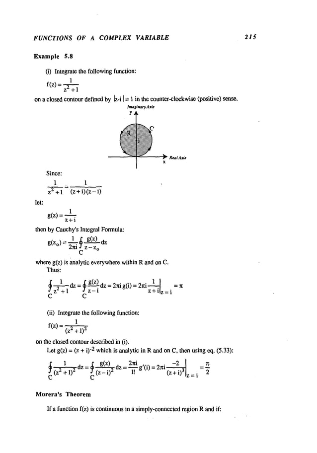
![FUNCTIONS OF A COMPLEX VARIABLE 217
Imaginary Axis
Y ~
C2
¯
"~0
.X
Real Axis
Fig. 5.15: Closed Path for Taylor’s Series
z = z2 where:
5.8 Taylor’s Expansion Theorem
If f(z) is an analytic functionat O,then there is apo
wer se
ries that converges in
side
a circle C2centeredat zo andrepresentsthe functionf(z) inside C1,i.e.:
f(z) = an(z- Zo)n
n=0
where:
f(n)(zo)
a n --~
n!
(5.35)
Proof:
Considera point zo wherethe function f(z) is analytic (see Fig. 5.15)¯ Let points z and
be interior to a circle C2, ~ beinga point ona circle C1centered at Zowhose
radius = ro
¯ Considerthe term:
1 1 1
~-z (~-Zo)-(z-z o) (~-zo)[1-z-z°]](https://image.slidesharecdn.com/advancedmathematicalmethodsinscienceandengineering-hayek-230318001731-2b30ece5/85/advanced-mathematical-methods-in-science-and-engineering-hayek-pdf-231-638.jpg)
![CHAPTER 5 218
1 1 1
Zo) z-zo
(~ - Zo)[1- ~_--~o]
Usingthe followingidentity, whichcan be obtained by direct division:
U
n
1 =l+u+u2+...+~ for
1-u 1-n
then:
1 I Z - Z
o (Z - Zo)
2 (Z - Zo)
n-1
~= ’l + +...+
E-Z E-Zo (E-Zo)
2 (E-Zo)
3 (E--Zo)
n
since:
I(z - zo)/({- Zo)l
(Z -- Zo)
n
(E - Z)(E - n
Multiplyingboth sides of the precedingidentity by f(E)/2xi dEand integrating on the
closed contour C1, one obtains:
1 f(E) dE - 1 f(E) d~ + (z- Zo) f(E)
C1 C1 Ci
(Z-- Zo) n-1 $ f(~) dE + (Z-- Zo) n~ f(~)
24~ (~ - o)~ 2~i J (~ - z) (~ o)
C1 C1
UsingCauchy’sintegral formulaeq. (5.33), one can showthat:
f(z) = f(Zo) + (z- Zo) f,(Zo) (z- Z
o)2
1! 2!
where:
Rn (Z-Zo)
n
= 24 ~
C1 (~ - z)( E - Zo)
n
Takingthe absolute value of R
n, then:
r n 2nMro =
_~ ro M(r)n
IRnl<-~ (ro-r)ro n r o-r r
o
__ f,,(Zo) + ... (z- Zo)n-1 f(n -1)(Zo)+ Rn
(n- 1)!
TheremainderR
n vanishes as n increases:
LimlR.lo 0 since r/r o < 1
Finally, the Taylorseries representation is given by:
~ f(n)(z°) (Z--Zo)
n
f(z)
n!
n=0
TheTaylor’s series representation has the followingproperties:
1. Theseries represents an analytic function inside its circle of convergence.](https://image.slidesharecdn.com/advancedmathematicalmethodsinscienceandengineering-hayek-230318001731-2b30ece5/85/advanced-mathematical-methods-in-science-and-engineering-hayek-pdf-232-638.jpg)
![FUNCTIONS OF A COMPLEX VARIABLE
r 219
2. Theseries is uniformlyconvergentinside its circle of convergence.
3. Theseries maybe differentiated or integrated term by term.
4. Thereis onlyone Taylorseries that represents an analytic function f(z) about
point z
o.
5. Sincethe function is annlytic at zo, then the circle of convergence
has a radius
that extendsfromthe center at Zoto the nearest singularity.
Example 5.9
(i) Expand
the function z in aTa
ylor’s se ries ab out Zo
= 0. Since:
f(n)(zo) 1
Iz=O
then the Taylorseries about zo = 0 is given by:
e z= ~ zn
n=0
Theradius of convergence,
p, is oo, since:
p= Lim[ an [= Lim]~-~oo
n-~**lan+ll n-->,~l n! I
(ii) Obtainthe Taylor’s series expansionof the followingfunction about Zo=
1
f(z) = z2 _
Usingthe series expansionfor (1.- u)"1, withu = z2/4:
oO
1 1 1 E (z’)2n
f(z)= 4 l_(Z)2_~ =-~" "2"
n=0
whichis convergentin the region]z 1<2. It shouldbe noted that the radius of
convergence
is the distance fromzo =0 to the closest singularities at z = +2, i.e. p = 2.
(iii) Obtainthe Taylor’sseries expansionof the function in (ii) about zo = 1
about Zo= -1.
Tofind the series aboutzo = 1, let ~ = z - 1, then the function f(z) transforms
1[ 1
1 =~" ~- 1 ~-3’
= + 3)
Expanding
f(z) about Zo = 1 is equivalent to expanding~ (4) about ~ = 0. TheTaylor
series for the functionsare as fgllows:](https://image.slidesharecdn.com/advancedmathematicalmethodsinscienceandengineering-hayek-230318001731-2b30ece5/85/advanced-mathematical-methods-in-science-and-engineering-hayek-pdf-233-638.jpg)
![CHAPTER 5 220
1 = 1 E (-1)n 3-’if"
convergent in <3
~+3 3
n=0
Thus, the twoseries have a common
region of convergence14 [ < 1:
~(~)=-"0 ~n+ 3--ff’~-~ )J c°nvergentinl4]<
and the Taylorseries representation of f(z) about o =1 be
comes:
f(z) -- --4n__~;01 + 3-’~-~J(Z- l)n convergentin Iz-ll
It shouldbe noted that the radius of convergence
represents the distance betweenzo =1
andthe closest singularity at z = 2.
Tofind the Taylorseries representationof f(z) aboutzo = - 1, let ~ =z + 1, then the
function transforms to ~(~):
l
1I 1 1 ]
~’(4)=(~+1)(~-3)=~ 4-3
Expandingf(z) about Zo = -1 is equivalent to expanding~(~) about = 0.The
Taylor
series for the functionsare as follows:
1 1 oo 4n
- ~-~- convergentin 141< 3
4-3 3 n=0
= E (-1)n 4n convergentin 141< 1
~+1
n=0
Thusthe two series, whenadded, convergein the common
region 14 1 < 1:
1 E I3-n~+l +(-1)nl4n convergentin[~,<
~(~) = - ~"n =
andthe Taylorseries representationof f(z) aboutZo=- 1 is:
=_1 ,~ r~l
1
convergent in lz+l [ 1
f(z) 4.Z~_n[_3n+l +(-1) n (z+l)
n <
Again,note that the radius of convergence
represents the distance between
zo = -1, and the
closest singularity at z =-2.](https://image.slidesharecdn.com/advancedmathematicalmethodsinscienceandengineering-hayek-230318001731-2b30ece5/85/advanced-mathematical-methods-in-science-and-engineering-hayek-pdf-234-638.jpg)
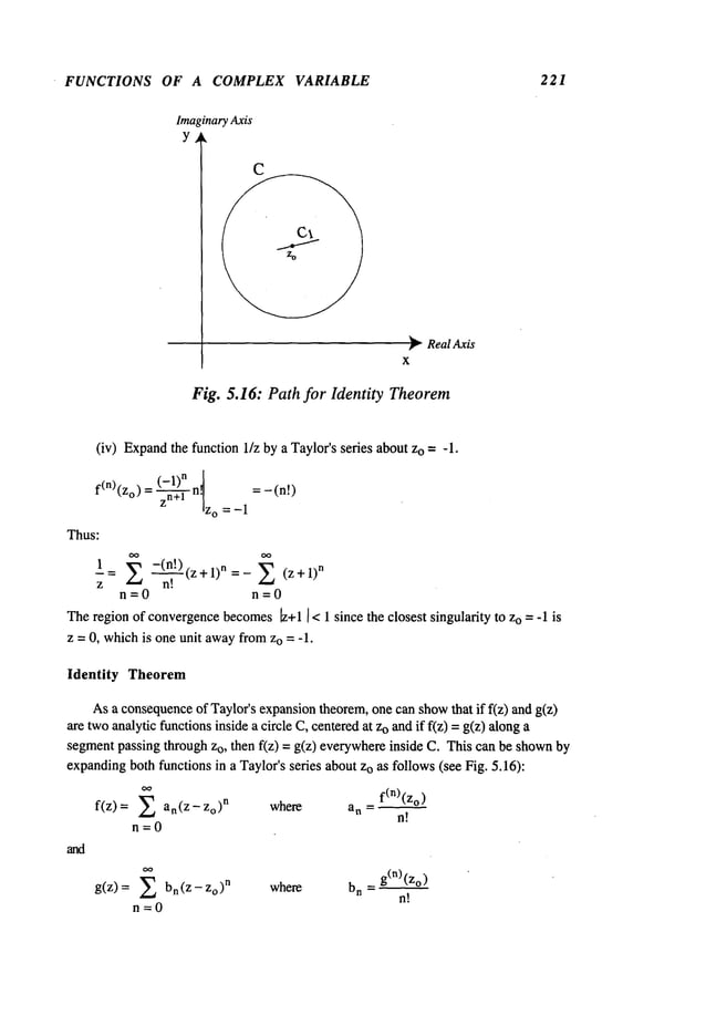
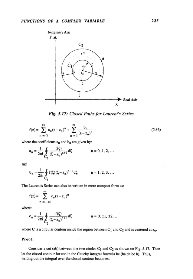
![CHAPTER 5 224
b a
2rtif(z)=
~~--~
f(
~)d
+~
--~ ~-
~---~ ~
f(
~)d f(~)d
+~--~
f(
~)d
C
2 a C
I b
=~--~f(~)
d~-~-~-~f(~)
C
2 C
1
The
expansion
onthe
contour
C2follows
that
ofa Taylor’s
series,
i.e.
for
~ onC2:
I I 1
Z-- Z
o
~ (~-Zo)-(Z-Zo) (~-zo)[1-~_--~-o]
1 Z -- Z
o
(Z -- o)n-I (Z -- o)n
= ~-~ +...+
~--Z o (~-- Zo)
2
(~- Zo)
n
wherethe division wasperformedon 1/(l-u) with:
lul= <1 f~, ~onC
2
Theexpansionon the contour C1can bc madeas follows:
1 1 1
~--~=(~-Zo)-(Z-Zo) = Z-Zo[l_~-Zo~
z-z
0
(~
-z)(~-
n
1 ~ - zo (~ - Zo) 2" (~ - Zo)
n-I
(~ - Zo)
n
Z-Z o (Z- Zo) 2 (Z-Zo) 3 "’" (Z_ zo)n (z- zo)n(z-
wherethe division wasperformedon 1/(1-u) with
lu~<l for ~onC
1
Thus,substituting these termsin the expansionfor f(z):
f(;) d;+(Z-Zo)~ f(;) dr+ +(Z-Zo>
n-1
2~if(z)
, ": °
C
2 C2 C2
1 :1 f(~)d~ +
+ 1Rn q (Z-Zo) (Z-Zo) "q" f(~)(~-z°)d~
C~
1
~ f(~)(~ - 2 d~ +
+(z- Zo)
3 C~
1
~ f(~)(~-Zo) n-1 d~+ 2Rn
...-I" (Z -- Zo)n Cl
Where
the remainderR
n can be shownto vanish as n ---)
d~](https://image.slidesharecdn.com/advancedmathematicalmethodsinscienceandengineering-hayek-230318001731-2b30ece5/85/advanced-mathematical-methods-in-science-and-engineering-hayek-pdf-238-638.jpg)
![FUNCTIONS OF A COMPLEX VARIABLE 225
nL.~lrn~[l Rn [ = Liml(z- Zo) n f(~) d~ I -->
n-->,,~[C2 ~ (~- Zo,)n+l (~ -
Liml2Rnl = Liml1 C~1 f(~) (~- z°)n d~[--~
n--->~* n~o] (Z - Zo) n ’~--’~"~
Example 5.11
(i) Obtainthe Laurent’sseries of the followingfunction abouto =0:
l+z
f(z) =
The functionf(z) is analytic everywhere
exceptat z --
Thefunction f(z) can be rewritten as:
1 1
f(z) =.~- +.~-y
In this case, it is already in Laurent’sseries formwherean =0, b
I = 0, b2 =1,
b3=1, and bn = 0 for n > 4.
(ii) ObtainLaurenfsseries for the followingfunction about o =0 valid in the
regionIzl >1:
1
f(z) =
1-z
Sincethe regionis definedbyIzl >1, then 1/Izl <1, thus, letting ~ = l/z, then:
f(z) =f(~-l) =1--= "-~-~--I ~ -- ~ ~ ~n = _ ~’~
~
n=0 n=0
whichis convergentfor I~1 < I. Thus:
f(z)
n=0
whichis convergentin the regionIzl > 1.
(iii) Obtainthe Laurent’sseries for the followingfunction about o =0,valid in the
regionIzl > 2:](https://image.slidesharecdn.com/advancedmathematicalmethodsinscienceandengineering-hayek-230318001731-2b30ece5/85/advanced-mathematical-methods-in-science-and-engineering-hayek-pdf-239-638.jpg)
![CHAPTER 5 226
1
f(z) = z2 _
Thefunction has twosingularities at z = +2. Since the function is analytic inside the
circle Izl=2,a Taylor’sseries canbe obtained(see Example
5.9). Forthe regionoutside
[z[ =2, oneneedsa Laurent’sseries representation. Factoringout z2 fromf(z):
1
f(z)= z2(1,4/z2)
then one can use the division of 1/(l-u) whereu = 4/z2:
O0
n=0
convergentover the region, 12/zI < 1. Thiscan be rewritten as:
1
2)_2(n+1)
f(z)=~- Z (z/
n=0 ¯
convergentoverthe region, Izl> 2.
(iv) Obtainthe Laurent’sseries for the functionin (iii) abouto =2 valid in the
regions:
(a) 0 Iz-21 <
4 (b) Iz-21
>4
Toobtain the series expansion,transfer the origin of the expansion
to zo = 2, i.e., let
11=z - 2 suchthat the functionf(z) transformsto ~’(11):
~(~) = 1
rl (11+4)
whichhas twosingularities at 11 =0 and 11 = -4. Thus,twoLaurent’sseries
corresponding
to ~(11)arerequired, one for 0 <I’ql <4 and onefor [’ql >4 as shown
in
Fig. 5.18.
(a) In the region R1, where0 < Irll < 4, onecan expand1 / 01 + 4) as follows:
OO
l = 1 = 1 Z
(rl+4) 4(1+11/4) 4
n
n=0
convergentin Irl/4] < 1. Thus,the Laurent’s series representation for ~(11)becomes:
oo (1) n (11)n-1
n=0
convergent
in 0 < I~ll < 4, since11~is not analytic at 11= 0.
Thus,the Laurent’s series about zo = 2 becomes:](https://image.slidesharecdn.com/advancedmathematicalmethodsinscienceandengineering-hayek-230318001731-2b30ece5/85/advanced-mathematical-methods-in-science-and-engineering-hayek-pdf-240-638.jpg)
![FUNCTIONS OF A COMPLEX VARIABLE 227
ImaginaryAxis
y
x
Real Axis
Fig. 5.18: Laurent’sSeries Expansionsin TwoRegions
1 o~ (z- 2)
n-I
f(z)=~-~ (-lln 4n-I
n=0
convergentin 0 < Iz - 2] < 4.
(b) In the region 2, w
here ~] >4,or 4/1~11 < 1
, one
mayfactor out "q from
the
function, such that:
oo
1 1 E ("-4)n
~(n)=n20 +4/ n)=~-r~=
0 n"
convergentin ¼/rll <1. Thus,the Laurent’sseries representation abouta3 = 0 is:
1 oo 4n+2
n=O
convergent
inI~II
> 4,or,
about
the
point
z
o =2 isrepresented
by:
I ~ 4
n+ 2
f(z) = ~-ff (-1)n (z "+2
n=O
convergent
in Iz - 21 > 4.
(v) Obtain theLaurent’s sedes ofthefollowingfuncfion about z~ =
1
f(z)=
(z-1)(z+2)
valid in the entire complex
plane: i.e. lzl <1; 1 <Izl < 2, andlzl >2.](https://image.slidesharecdn.com/advancedmathematicalmethodsinscienceandengineering-hayek-230318001731-2b30ece5/85/advanced-mathematical-methods-in-science-and-engineering-hayek-pdf-241-638.jpg)
![CHAPTER 5 228
Thefunction f(z) can be factored out in terms of its twocomponents:
1 ~I 1 1 ]
f(z)
=(z-
l~(z
+ =
’z
-- I
z ~ 2"
(a) In the regionIzl <1, the functionis analytic thus:
= - E zn convergentin Izl < 1
(z- 1)
n=0
1 1 ’~ (-z)
n
convergent
in Izl < :2
(z + 2) 2 2
n
n=0
and, the sumof the two expansions becomes:
f(z)= -1 ~ [1+ (-1)nlz
n
... _.-:’:Tw~ ! convergentin Izl < 1
3
n’7_-0L
(b) Expansion
of f(z) in the region 1 < Izl
Since1/(z+2)is analytic inside Izl =2, then a Taylor’sseries is needed,while1/(z-l)
is not analytic inside Izl = 2, which
requires a Laurent’sseries:
I
= E z-n-I
convergentin Izl > 1
1"-~
(z
n=0
1 =_.I ~-~ (-z)
n
(z +2) 2 "-" 2
n
convergentin Izl <2
n=0
Thus, the addition of the two series convergein the common
region of convergence:
f(z) z-n-1 + (-z)n
_
2n+l
convergentin 1 < Izl < 2
(c) Expansion
of f(z) in the region Izl>
Thefunction 1/(z+2) and1/(z~l) are not analydcinside and on Izl =2, thus
Laurent’sseries is necessaryfor both:
1
/1"-’-’’~(z - =~ z-n-1
convergentin Izl >1
n=0
1
)2’’~-(z + = ~ (- 1)n 2n z-n-I
convergentin Izl >2
n=0
Thus,the series resulting from the addition of the twoseries convergesin the common
region Izl> 2 becomes:](https://image.slidesharecdn.com/advancedmathematicalmethodsinscienceandengineering-hayek-230318001731-2b30ece5/85/advanced-mathematical-methods-in-science-and-engineering-hayek-pdf-242-638.jpg)
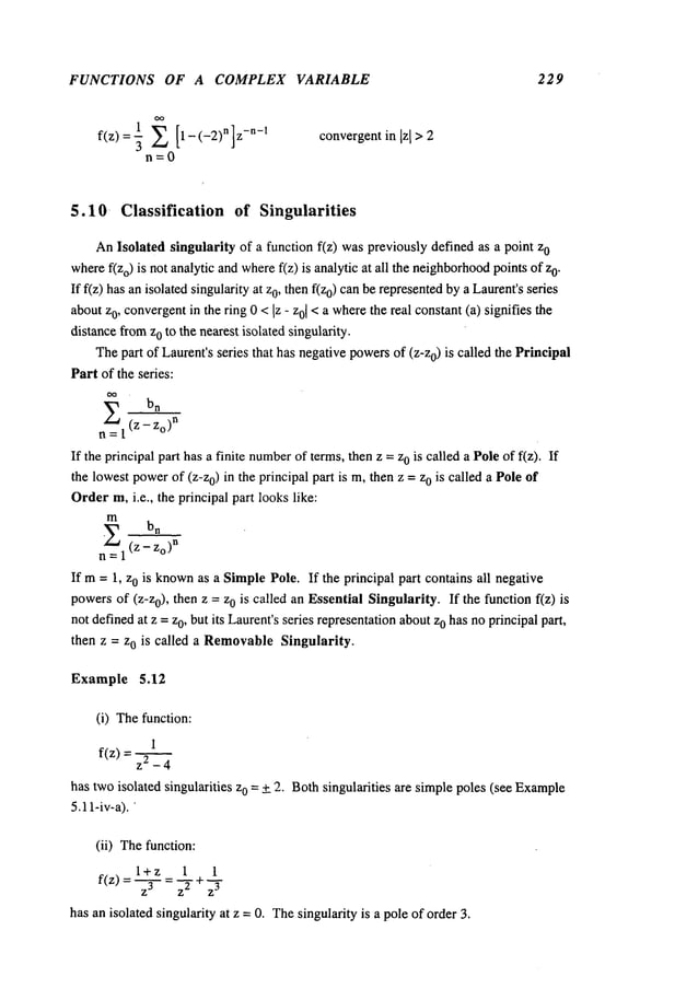
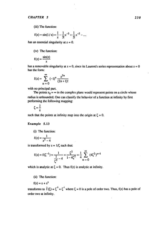
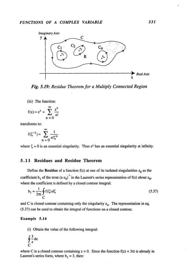
![CHAPTER 5 234
f(z)= g(z) = E g(n)(z°)(z-z°)n-m
(Z - o)m n=O
Fromthis expansion,the coefficient b1 can be evaluated in terms of the (m-l)" derivative
of g:
bt = g(m-1)(z°) (5.39)
(m- 1)!
If f(z) is a quotientof twofunctionsp(z) andq(z):
f(z) = p(z)
q(z)
wherethe functions p(z) and q(z) are analytic 0 and p(z0) ¢ 0,then one c
an find the
residue off(z) at o if q(zo) =
0.Sin
ce thefunc
tions p(z)and q
(z) are analy
tic at z o, then
onecan find their Taylorseries representationsabout z0 as follows:
p(z)= P(n)(z°)(z-z°)n
n!
n=O
q(z) = ~ q(n)(zo) (z- Zo)
n
n!
n=0
Variouscases canbe treated, depending
on the formthe Taylorseries for p(z) and q(z)
wherep(z0) ¢
(i) If q(zo) =0 andq’ (zo) * 0, then f(z) has a simplepole at o, and:
g(z) = (z- Zo) f(z) P(Z°) + P’(Z°)(z- z°) + "’"
q’(Zo)+q"(Zo)(z - zo) ] 2
Thus,the residue for a simplepole can be obtainedby direct division of the twoseries,
resultingin’.
bl = g(zo) = P(z°) (5.40)
q’(z
o)
(ii) If q(zo) =0 andq° (Zo)= 0 ando) ¢ 0, then f(z) has apole
oforder
2, where:
p(Zo)
+p’(zo)
(z-Zo)
g(z) = (z - 2 f(z) =
q"(Zo)/ 2 +q’(Zo)(Z- zo) / 6
Dividingthe twoinfinite series to include termsup to (z-z0) and differentiating the
resulting series results in:](https://image.slidesharecdn.com/advancedmathematicalmethodsinscienceandengineering-hayek-230318001731-2b30ece5/85/advanced-mathematical-methods-in-science-and-engineering-hayek-pdf-248-638.jpg)
![FUNCTIONS OF A COMPLEX VARIABLE 235
bt = g’ (Zo.__~) = 2p’(Zo)p(zo)q"(Zo) (5.41)
1! q"(Zo)3 [q,,(Zo)]
~
(iii) If q(z0) =q’(z0) 0,, q~m
l)(z
0) ¢’~
..... 0, and q (z 0) ¢ 0, then f(z) has a pole
of order msuchthat:
g(z) =(z - Zo)rn f(z) P(z°)+ P’(z°)(z o)+ .. .
q(m)(zo)/ m[+q(m+l)(zo)(Z
- Zo) / (m
then, in order to evaluate b1, onemustdivide the twoinfinite series and retain termsup to
(Z-Zo)
mlin the resulting series. Differentiating the series (m-l) timesand setting z = 0
one obtains the valueof bl:
b1 = g(m-l)(z°) (5.42)
(m- 1)!
Example 5.16
Obtainthe residuesof eachof the followingfunctionsat all its isolated singularities:
Z
2
(i) f(z)=
(z+1)(z-
At zo = - 1, there is a simplepole, wherethe residueis as follows:
(-1)2 t
r(-1)
=g(-1)
=(z+1)f(Z)lz
=(-1
- 2-’~
-~
=- ~
Atzo = 2, there is a simplepole, wherethe residue is as follows:
(2) 2 4
r(2) = g(2) =(z - 2)f(Z~z=(2+1--~ = ~
e
Z
(ii) f(z)
Z
zo =0 is a pole of order 3. Therefore,g(z) is definedas:
g(z) = z3f(z) z
andthe residueis as follows:
r(0) g’(0~) =1 e0= 1
2! 2 2
z+l
(iii) f(z)
sin z
This function has an infinite number
of simplepoles, Zn = nr~, n = 0, +1, +2..... Let
p(z) = z+1 andq(z) = sin
Thus,using the formula(5.40):](https://image.slidesharecdn.com/advancedmathematicalmethodsinscienceandengineering-hayek-230318001731-2b30ece5/85/advanced-mathematical-methods-in-science-and-engineering-hayek-pdf-249-638.jpg)
![CHAPTER 5 236
r(nr0=z+~ = nr¢+l
sin’zlnn cos (nr0
-- = (-1)n (nrc +
5.12 Integrals of Periodic Functions
Theresiduetheorem
canbeusedto evaluateintegrals of the following
type:
= J F(sin0, cos0) (5.43)
0
where
F(sin0, cos0) is a rationalfunctionof sin 0 andcos0, andis bounded
onthe path
of integration.
Using
the parametrictransformation:
z = e
i0
which
transforms
the integralto oneona unit circle centered
at the origin, andusingthe
definitionof sin 0 andcos0, onegets:
sinO= ~i[z- ~] CosO= l[z+
-1 ]
2L zJ
andthedifferentialcanbewrittenin termsof z:
dO=-i
~z (5.44)
Z
Theintegralin eq. (5.43)canbetransformed
to the following
integral:
= ~ f(z)
I
C
where
f(z) is a rationalfunctionof z, which
is finite onthe pathC, andCis theunit
circle centered
at the origin. Letf(z) haveNpolesinside theunit circle. Theintegral
theunit circle canbeevaluated
bytheresiduetheorem,
i.e.:
N
= ~ f(z)dz = 2hi E
I (5.45)
C j=l
where
rj’s aretheresidues
at all theisolatedsingularities
of f(z) insidetheunit circle
Example 5.17
Evaluate
the following
integral:
2r~
~ 2dO
2+cos0
0
Using
the transformation
in eq. (5.44), the integral becomes:](https://image.slidesharecdn.com/advancedmathematicalmethodsinscienceandengineering-hayek-230318001731-2b30ece5/85/advanced-mathematical-methods-in-science-and-engineering-hayek-pdf-250-638.jpg)
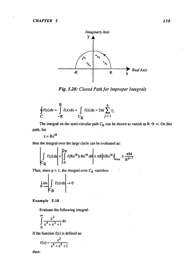
![FUNCTIONS OF A COMPLEX VARIABLE 239
1
If(z)l ~ ~ when Izl >>
~
hencep = 2 and the integral over C
Rvanishes. Thefunction f(z) has four simplepoles:
l+i’~ -1+i-x/~ 1- i-~/’~ -1-i-~
Z1 - Z2 = Z 3 = ~ Z4 =
2 2 2 2
wherethe first twolie in the upperhalf plane. Theresidue of f(z) at the poles1 and z2
becomes:
l+i-~) 1+ia/’~
r(zl = --2 = z~z~Lim
(z - 1)f(z) =4i-~-
= 1-i4
r(z2 = -1 Lira (z - 2)f(z) =4i-~-~-
2 z--,z
2
Thus,usingthe results of eq. (5.47), the integral can be evaluated:
x
2
1 x2 1 _ .F1 + ia/’~ 1-i~/-~]_ ~
dx=- f x4 x 2 dx=’~2~lk 4"~+
- x~ + x2 + 1 2 + + 1 4i’~ ]- 2~/~
0 "-~
5.14 Improper Real Integrals Involving Circular Functions
Theresidue theoremcan also be used to evaluate integrals havingthe followingform:
~f(x) cos(ax) dx for a
~f(x) sin(ax) for a > 0
~ f(x)e iax dx for a > 0 (5.48)
wheref(x) has nosingularities on the real axis and a is positive. Let f(z) be an analytic
functionin the upperhalf planeexceptfor isolated singularities, suchthat:
[f(z)[< Mlzl
-p where p > 0 for Izl >> 1
Sincethe first twointegrals of eq. (5.48) are the real andimaginary
parts of the integral
eq. (5.48), oneneedsto treat onlythe third integral.
Performingthe integration on f(z) iaz on t he closed contours shown i
n Fig. 5 .20,
then:](https://image.slidesharecdn.com/advancedmathematicalmethodsinscienceandengineering-hayek-230318001731-2b30ece5/85/advanced-mathematical-methods-in-science-and-engineering-hayek-pdf-253-638.jpg)
![CHAPTER 5 240
Fig. 5.21: Approximation for Jordan’s Lemma
R
~f(z)eiaZdz = f f(x)eiaXdx+ f f(z)eiaZdz
C -R C
R
Onemust nowshowthat the integral vanishes as R--> ~. This proof is knownas
Jordan’s Lemma:
Lira ~ f(z)eiaZdz --*
R-->,~ CR
Let z = Rei° on C
R, then the integral becomes:
j
" f(Re
i0) eia Rei°ei0 iR dO=iRf f(Re
i0) eiaR[c°s0+i
sin 0]ei0d0
0 0
Thus,the absolute value of the integral on C
Rbecomes:
ff(z)eiaZdz =R f(Rei0)ei[aRc°s0+0le-aRsin0d0 < e-aRsin0d0
C
R
Thelast integral canbe evaluatedas follows:
~ ~/2 rtt2
~e-aRsin0d0=2 J" e-aRsin0d0<2 ~ e-2aR0/~d0= ~._~_(a_e
-aR) aR
0 0 0
wherethe followinginequality wasused (see Fig. 5.21):
2O
sin 0 _>-- for 0 < 0 < ~z/2
Thus:](https://image.slidesharecdn.com/advancedmathematicalmethodsinscienceandengineering-hayek-230318001731-2b30ece5/85/advanced-mathematical-methods-in-science-and-engineering-hayek-pdf-254-638.jpg)
![FUNCTIONS OF A COMPLEX VARIABLE 241
whichvanishesas R--) ,,~, since a > 0 andp > 0. It shouldbe notedthat the integral
becomes
unbounded
if a < 0, or equivalently, if a >0 and the circular path is takenin the
lower half plane. Thus:
00 N
P.V. ~ f f(x)e iax dx = 2r:i 2
P.V. ff(x)cos(ax)dx Re2~i 2 rj =- 2~l m rj
k j=l J kj=l J
P.V. f(x) sin(ax) dx lm2hi2 rj = 2~ Re rj (5.49)
L j=l Lj= .J
where
the rj’s representthe residuesof the Npoles of {f(z) iax} in the upper h
alf plane~
Example 5.19
Evaluatethe followingintegral:
f cosX
0
Sincef(z) = 4 + !)"1, then If(z)l _<"Pon C
Rfor R >>
1,whe
re p = 4 and a = 1.
Thefunction f(z) has four simplepoles:
l+i -l+i -1-i 1-i
z 1=~ z2=~ z3= ~ z4=’~"
wherethe first twolie in the upperhalf plane, note that Zl4 =z24 = -1. Thus,the integral
can be obtainedby eq. (5.49):
1 cos_..~.xdx- -rdm[rl +r~]
wherethe residue, z1 is calculated fromp/q’ for simplepoles: ,
and similarly for the secondpole z2:](https://image.slidesharecdn.com/advancedmathematicalmethodsinscienceandengineering-hayek-230318001731-2b30ece5/85/advanced-mathematical-methods-in-science-and-engineering-hayek-pdf-255-638.jpg)
![CHAPTER 5 242
_ ~ I- i c_(i+~)/~f~
r(z2)= 4 =4-~
Thus, the integral I can be solved:
nm m
I = -~- e- [cos m+ sin m]
5.15 Improper Real Integrals of Functions Having
Singularities on the Real Axis
Functionsthat havesingularities on the real axis can be integrated by deformingthe
contourof integration. Thefollowingreal integral:.
b
where
b
f(x)dx
f(x) has a singularity onthe real axis at x = c, a <c <b is definedas follows:
[ci
I
ff(x)dx=Lima
e-~o a f(x)dx
+i Lcj’+
f(x)dx
Theintegral on [a,b] exists iff the twopartial integrals exist independently.
If either or
bothlimits as e "-> 0 and 8 --> 0 do not exist but the limit of the sumof the twointegrals
exists if e = 8, that is if the followingintegral:
Lim f(x)clx
f(x)dxe~°L c + e
exists, then the value of the integral thus obtained is called the CauchyPrincipal
Valueof the integral, denotedas:
b
P.V. ~ f(x)dx
-a
Example 5.20
(i) Evaluatethe followingintegral:
2
~x-1/3dx
-1
Notethe function f(x) -- "lt~ is singular at x =0.The
refore:](https://image.slidesharecdn.com/advancedmathematicalmethodsinscienceandengineering-hayek-230318001731-2b30ece5/85/advanced-mathematical-methods-in-science-and-engineering-hayek-pdf-256-638.jpg)
![FUNCTIONS OF A COMPLEX VARIABLE 243
2
J
~X
-1/3
(ii) Evaluatethe followingintegral:
2
~x-3dx
-1
-3
Thefunction f(x) = x is singular at x =
-11x-~ _a_l x-3dx a~0|L0a+~
:± im[l- l+±umF4-11
2 ~--,oL~ ] 2 ~-~oL8
~ 4J
Neitherintegralexists for Eand5 to vanishindependently.
If onetakesthe P.V.of the
inte~a]:
P.V. x-3dx =Lira x-3dx + x-3dx = ~
~°L ~1
8
-1 - O+e
Improper
integrals of function on the real axis
~ f(x)dx
wheref(x) has simplepoles on the real axis canbe evaluatedby the use of the residue
theoremin the CauchyPrincipal Valuesense.
Let xl, x2 .... x
n be the simplepolesof f(z) onthe real axis, andlet 1, z2 ..... z mbe
the poles of f(z) in the upper-halfplane. Let Rbe the semi-circular path w
ith a radius
R, sufficiently large to include all the polesof f(z) onthe real axis andin the upper-half
plane. Thecontouron the real axis is indentedsuch that the contourincludes a semi-
circle of small radius = e aroundeach simplepole xj as shown
in Fig. 5.22.
Thus,onecan obtain the principal value of the integral as follows:
fXl_~Rl~ f x2~ -1~ i ~ m
+ + +f +...+ +J" f(z)dz= f(z)dz=2~iZr
j
C 1 x 1 + 8 C
2 x n + e C
R
j =1](https://image.slidesharecdn.com/advancedmathematicalmethodsinscienceandengineering-hayek-230318001731-2b30ece5/85/advanced-mathematical-methods-in-science-and-engineering-hayek-pdf-257-638.jpg)
![CHAPTER 5 244
ImaginaryAxis
Y
-R Xl x2 xn R
#" Real Axis
X
Fig. 5.22: Closed Path for Improper Integrals with Real
and Complex Poles
where
the contoursCj are half-circle paths in the clockwisedirection andrj’s are the
residuesof f(z) at the polesof f(z) in the upperhalf planeat zj. Thelimit as R--) co
e --) 0 mustbe taken to evaluate the integrals in CauchyPrincipal Valueformon R and
onCjforj=l, 2 ..... n.
If the functionf(z) decaysfor [z[ "-) co as follows:
If(z)l < Mlzl
-p where p > 1 for Izl >> 1
then, it wasshown
earlier that:
Since
the furiction f(~) hassimplepolesonther~al axis, thenin the neighborhood
each real simplepole Xj, it has one term with a negativepoweras follows:
f(z)= rj +g(z)
where
g(z) =the part of f(z) that is analyticat xj, andrj* are the residuesof f(z)
Thus,the integral over a small semi-circular path aboutxj becomes
in the limit as
the radius e -> 0:
Lim S f(z)dz = Llmlrj f dz S ]
¯ * ~ + g(z) dz = -Tzlrj
e--+0 e-~0/ ~ z-x
3
Cj L Cj Cj
wherethe results of Example
5.6 wereused.
Thus,the principal valueof the integral is givenby:](https://image.slidesharecdn.com/advancedmathematicalmethodsinscienceandengineering-hayek-230318001731-2b30ece5/85/advanced-mathematical-methods-in-science-and-engineering-hayek-pdf-258-638.jpg)
![FUNCTIONS OF A COMPLEX VARIABLE 245
P.W.
oo m n
--~ j=l j=l
(5.50)
Example 5.21
Evaluatethe followingintegral:
~ +a2) [Y~x(x 2 + a2) dx~
--~ x(x
2
fora> 0
e
iz
Thefunction z(z2 + a2) has three simple poles:
x1 = 0, z~=ia, z~=-ia
Toevaluate the inte~al, one needsto evaluate the residues of ~e approp~atepoles:
(z- ~)e
~z _
q (Zl) = z(z2 + a2) z I = ia 2a2 ea
z e
iz
r;(xl) = z~z~--a2)’lz = x1 =0
Thus:
P.V. f sin x
X(X
2 + a
2)
1
dx = lm[2ni{2a~ea
} + ~zi{~2}] = ~-2 [1 - e-a
]
5.16 Theorems on Limiting Contours
In section 5.13to 5.15 integrals on semi-circularcontours in the upperhalf-plane
with unbounded
radii wereshown
to vanish if the integral behavedin a prescribed manner
on the contour. In this section, theoremsdealing withcontours that are not exclusivelyin
the upperhalf-planeare explored.
5.16.1 Generalized Jordan’s Lemma
Considerthe followingcontourintegral (see Fig. 5.23):
f eaZf(z)dz
CR
wherea = b e~c, b > 0, c real andC
Ris an arc of circle describedby z =Re
i0, whoseradius
is R, and whoseangle0 falls in the range:](https://image.slidesharecdn.com/advancedmathematicalmethodsinscienceandengineering-hayek-230318001731-2b30ece5/85/advanced-mathematical-methods-in-science-and-engineering-hayek-pdf-259-638.jpg)
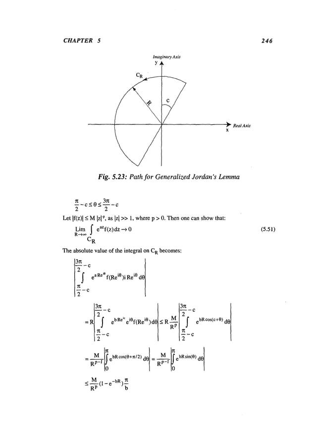
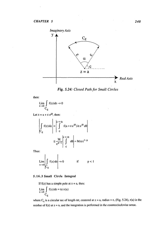
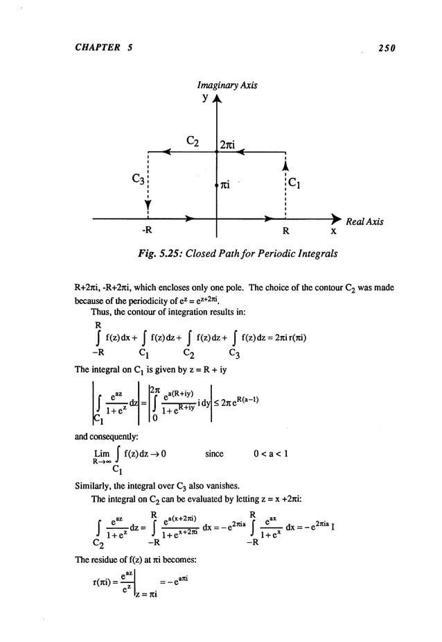
![FUNCTIONS OF A COMPLEX VARIABLE 251
Imaginary
Axis
Y
RealAxis
Fig. 5.26: Closed Path for Periodic Integrals
Thus,as R-->
I - e2niaI =2~i(-enia )
I = 2~i (enia) =
e2nia - 1 sin(an)
Theevaluation of improperintegrals of the form:
j
" f(x)
0
wheref(x) is not an evenfunction, cannotbe evaluated byextendingthe straight path
[-oo,~]. Thus,one mustchooseanother contourthat wouldduplicate the original integral,
but with a multiplicative constant.
Example 5.23
Evaluatethe followingintegral:
oo
j’dx
I= x3 +1
0
Sincethe integral path cannotbe extendedto (_oo), then it is expedientto choosethe
contour as shownin Fig. 5.26. Thepath C
1, where0 = 2~r/3, waschosenbecause along
that path, Z3 : (10 e2~ti/3) 3 = ~)3 andis real, so that the functionin the denominator
doesnot
change.
Thefunction f(z) = 1/(z3+l) has three simplepoles:
1 +i~f~ 1- i~f~
Z 1 = ~, Z
2 = -1, and z3 -
2 2](https://image.slidesharecdn.com/advancedmathematicalmethodsinscienceandengineering-hayek-230318001731-2b30ece5/85/advanced-mathematical-methods-in-science-and-engineering-hayek-pdf-265-638.jpg)
![FUNCTIONS OF A COMPLEX VARIABLE 253
ImaginaryAxis
Y
BranchCut
Real Axis
Fig. 5.27: Closed Path for Logarithmic Integrals
the poles of f(z) in the upper-halfplanebe 1, z2 ..... z m.L
et CRbe asemi-circular
contour, radius = Rand C
Obe semi-circular contourradius = e in the counter clockwise
sense. Thus,the integral over the closed path becomes:
in
~f(z)logzdz={L~I-C~o
+j2+~}f(z)logzdz=2~iCR rj(zj). 1
whererj’s are the residuesof [f(z) log z] at the polesof f(z) in the upper-halfplane.
integral on C
Oin the clockwisedirection can be evaluatedwherez = eei°:
Thus,sincethe liinit of f(z) is finite as z goesto zero, then:
f f(z) log z dz
Liin 0
~--~0
C
o
Theintegral on C
Rcan be evaluated, wher~z = R
whichvanishes whenR --> ~, so that:](https://image.slidesharecdn.com/advancedmathematicalmethodsinscienceandengineering-hayek-230318001731-2b30ece5/85/advanced-mathematical-methods-in-science-and-engineering-hayek-pdf-267-638.jpg)
![CHAPTER 5 254
Lim| f(z) log z dz -~ since p > 1
R-~,**
CR
Theintegral on L
1 can be evaluated as follows:
z=pein=-p dz:-dp
log z = log p +i~
~ f(z)logzdz =-j" f(-p)[log0 + ix]d0
L1 R
Theintegral on L
2 can be evaluated in a similar manner:
z = O dz = dp log z = log O
R
~ f(z)logzdz= ~ f(0>logDd0
L2 e
Thetotal integral, after substituting if-0) = f(0), becomes:
R R m
2~ f(p)logpdp + ix~ f(p)dp = 2~i
j=l
Takingthe limits e --) 0 and R--) .0 one obtains uponsubstituting x for
~ ~o
m
~ f(x) logxdx=---i~ f f(x)dx + r~i (5.53)
2
0 0 j=l
If the function f(x) is real then the integral of f(x) log x mustresult in a real value.
integral onthe right side is also real, hencethis termconstitutes a purelyimaginary
number.For a real answer, the imaginarynumberresulting fromthe integral term must
cancel out the imaginarypart of the residue contribution. Thus,one can then simplify
finding the final answerby choosingthe real part of the residue contributions on the right
side of equation(5.53), i.e.:
f f(x)logxdx:Re /fi ~ rj :-r~Im rj
0 L j:l ] Lj=l j
Example 5.24
Evaluatethe followingintegral:
~logx dx
x2 +4
0](https://image.slidesharecdn.com/advancedmathematicalmethodsinscienceandengineering-hayek-230318001731-2b30ece5/85/advanced-mathematical-methods-in-science-and-engineering-hayek-pdf-268-638.jpg)
![FUNCTIONS OF A COMPLEX VARIABLE 255
Thefunction f(z) = 1/(z2 + 4) has twosimplepoles at:
z1 = 2i =2 e
in/2, z2 = -2i
Theresidueat z1 is:
r(2i) = log
2z z = 2i
also f(x) is real and:
1
If(R)] < -- with p = 2, for R >> 1
R
p
Thus:
,ox I
. =- i__~.n d.__._~_x+ in -
X
2 + 4 taX 2 X2 + 4 -ff 1 ~---J
0 0
since:
fd~x n
x2+4 =~
0
then:
flogx , i~ ~ . ~ .log2 ~
0
_ log(2i) ~ii .n ~ il°g2
- 4-----~ = (log2 + ~) =-if-
It is thus shown
that the imaginary
parts of the answercancelout since fix) is a real
function. Or, one coulduse the shortcut, to give:
fx2 + 4 ux -t--~--] = ~- log 2
0
If the function f(x) has n simplepoles on the real axis, then oneindents the contour
over the real axis bya smallsemi-circle of radius e, so that the path integral becomes:
{-~ j--~l R m
+ f+f +f+f .f(z)logzdz=2rtiZrj(zj)
Cj Co e C
R
j=l
wherethe function has mpoles at zj in the upperhalf planeas well as n simplepoles at xj
on the real axis, andCj are the semicircularpaths aroundxj in the clockwisedirection.
Eachsemi-circularpath contributes - in rj* (xj) so that the integral becomes:
~f(x)logxdx=-2 f(x)dx+ni q*(xj/ (5.54)
0 0 j=l j=l](https://image.slidesharecdn.com/advancedmathematicalmethodsinscienceandengineering-hayek-230318001731-2b30ece5/85/advanced-mathematical-methods-in-science-and-engineering-hayek-pdf-269-638.jpg)
![CHAPTER 5 256
Once
againif f(x) is real then the integral of f(x) log x mustbe real and equation(5.54)
canbe rewritten:
~ f(x’ l°g x dx=- r~Im[j--~l rj(zJ’ +~ j --~lr~(xJ)]0
Example 5.25
Evaluatethe followingint~gral:
~logx dx
x2 -4
0
Thefunction has two simplepoles at x = + 2 and no other poles in the complexplane.
Sincethe branchcut is definedfor - r~/2 < 0 < 3r~/2, then these are describedby:
xI =-2=2e
in, x2=2e
i0
Theresidues at xI andx2 are:
=
1 . ~ log2
r* (2e
in) logzl = - (log 2 + in) =
z-21z=-24 4 4
r*(2e°) = l°g_z
I = ¼(log2)
z+:Zlz= 2
Sincef(x) is real the integral has the followingsolution:
=-5Im rj*(xj) =-~Im -i-~ ~ ~--~.-.~=~-
~f(x) logx
0
Integrals involving (log x)n can be obtainedfromintegrals involving (log x)k, k = 0,
1,2..... n-1. Thefollowing integral can be evaluated:
~f(x) (log n dx
0
wheren = positive integer, f(x) is an evenfunction andhas no singularities on the real
axis and:
M
If(z)l-<- p > 1, for Izl >>1
Using the samecontour shownin Fig. 5.27, then one can showthat:
m
{~l-Jo+~+~ }f(z)(lOgz,ndz:2ni~rj(zj)L
2 C
R
j=l](https://image.slidesharecdn.com/advancedmathematicalmethodsinscienceandengineering-hayek-230318001731-2b30ece5/85/advanced-mathematical-methods-in-science-and-engineering-hayek-pdf-270-638.jpg)
![CHAPTER 5 258
~ m
1 ~.I , n-k ~
f ~ ~f f(x)(logx)k (5.55)
f(x)(1ogx)n dx = ~ti ~
tn - k).’K.,~
0 j=l k=0 0
Thusthe integral in (5.54) canbe obtained as a linear combination
of integrals involving
(log x)k, withk =0, 1, 2 ..... n - 1.
Example 5.26
Evaluatethe followingintegral:
f dx
~ x~+4
0
fix) has twosimple poles at +2i and -2i. Usingthe resul~ of Example
(5.24), and
(5.55):
x~ + 4 dx = i~ r(2i)
(i~) 2 f(x)dx + 2ig f(x) logx
0
~e residue can be derived as:
2z 2i 4i
Usingthe results of Example
5.21 and eq. (5.55):
~x~+4 4
0 0
so that:
~ x)2 { ~(@)4 } ~{
[ 0o? dx = i~ - Oog~ - + ~ ~o~ ~ - (i~ ~ f~l + ai~ lo~ ~1
~ x~+4 4 4
0
=~[(log2) ~ + ~
Or, since fix) is real, the integral of f(x) mustbe real, there%re
onlythe real p~ of
right side needsto be computed,
i.e.:
~ (l°gx)2 dx =-nlm[r(2i)]+ ~2 f 1
~ x~ +4 ~ ~ ~
Oog
2): +
0 0
= ~[(Iog2)2 +](https://image.slidesharecdn.com/advancedmathematicalmethodsinscienceandengineering-hayek-230318001731-2b30ece5/85/advanced-mathematical-methods-in-science-and-engineering-hayek-pdf-272-638.jpg)
![FUNCTIONS OF A COMPLEX VARIABLE
ImaginaryAxis
Y
¯
Fig. 5.28: ClosedPathfor Integrals with x
a
259
Branch Cut
F RealAxis
x
5.19 Integrals of Functions Involving x
a
Integrals involving xa, whichis a multi-valuedfunction, can be evaluated by using
the residue theorem.Considerthe following integral:
OO
~ f(x)x
a a > (5.56)
dx -1
0
wheref(x) has nosingularities onthe positive real axis, anda is a non-integerreal
constant. Toevaluate the integral in (5.56), the integrand is made
single-valued
extendinga branchcut along the positive real axis, as is shown
in Fig. 5.28, suchthat
the principal branchis definedin the range0 < 0 < 2~. Let the poles of f(z) be z], 2 ....
zmin the complexplane and:
M
If(R)l_< with p> a+l, for R>> 1
Thecontouron C] is closed by addinga circle of radius = R, a line contouron C2
and a circle of radius = e, as shown
in Fig. 5.28. Thecontouris closed as shown
in such
a waythat it does not cross the branchcut andhence, the path integration stays in the
principal Riemann
sheet. Thus:](https://image.slidesharecdn.com/advancedmathematicalmethodsinscienceandengineering-hayek-230318001731-2b30ece5/85/advanced-mathematical-methods-in-science-and-engineering-hayek-pdf-273-638.jpg)
![FUNCTIONS OF A COMPLEX VARIABLE 261
Ima~maryAxis
Y
CR
Co o ci ci c~ / ~
J " ~ ~~~~--r Real Axis
R R X
Fig. 5.29: ClosedPath for Integrals with xa and Real Poles
Example 5.27
Evaluatethe followingintegral:
~
xl/2
x--~S+
1
dx
0
Let f(z) = 1/(z2 + 1), whichhas twosimplepoles:
zI =i =ein/2 z2 =-i =e
3ird2
wherethe argumentwaschosenappropriate to the branch cut. Theresidues become:
z1/2 1__ ei~/4 z1/2 = _ 1__e3ir~/4
q(i) =-~zi = 2i r2(i) =-~-z
2i
Since a > -1 and:
1
If(z)l as [z] >> 1 where p = 2 > 1/2 +1
R
p
then the integrals on C
Rand C
Ovanishas R--> ,~ and e --> 0 respectively. Thus:
~ x1/2 = 2~:i. r~l (ei;~/4 -e3in/4)]--~cos(~14)
~
x-~+l dx 1-e
rt~L2i"
-
0](https://image.slidesharecdn.com/advancedmathematicalmethodsinscienceandengineering-hayek-230318001731-2b30ece5/85/advanced-mathematical-methods-in-science-and-engineering-hayek-pdf-275-638.jpg)
![CHAPTER 5 2 62
If f(x) has simplepoles at xj onthe positive real axis then onecan indent the contour
on the positive real axis at eachsimplepole xj, j = 1, 2 .... n, as shown
on Fig. 5.29¯
Onecan treat one indented contourintegration on Cj and C
i. Since xj is a simplepole of
f(x), then its Laurent’sseries aboutxj is:
f(z)= rj + ~ ak(Z-XJ)
k
Z-Xj k=0
whererj is the residue of f(z) at the simplepole xj. Because
the pole falls ona branchcut,
then its location must be appropriate to the argumentdefined by the branchcut. Thus,
for the pole abovethe branchcut, its location is xj. Forthe pole belowthe branchcut,
its location is givenbyxj e
TM.
Onthe contoursC
i, let z-xj = e ei°:
01-
r. ~’ ]
=!l
"J’^+
__~0 J
ei°)aieei°
f f(z)z
adz ak(eeiO) (xj +e dO
e e
10
k
Limf f(z)z adz = -i~z(xj) a rj
~-->0
ci
Thecontouron Cj canbe treated in the samemanner¯
Let z - xj e2hi =13 ei0 then:
Limf f(z)z adz = -i~(xj) a e2nairj
e--->0
cj
Thus, the sumof the integrals on Cj and C~becomes:
{~+f }f(z)zadz=-i~r;(xj)(l+e
2naj)
c3 cj
wherethe rj s are the residues of {f(z) a} at t he poles xj o n Lr T
hus:
ff(x)xadx= 2~i ~i (l+e2Zai) ~ *
1 - e2nai rj ~ 1 - e
2~tai rj
0 j=l j=l
m n
-~ e-ani ~ rj +~cotan(Tza)~
sin(a~)
j=l j=l
(5.58)](https://image.slidesharecdn.com/advancedmathematicalmethodsinscienceandengineering-hayek-230318001731-2b30ece5/85/advanced-mathematical-methods-in-science-and-engineering-hayek-pdf-276-638.jpg)
![FUNCTIONS OF A COMPLEX VARIABLE 263
5.20 Integrals of Oddor AsymmetricFunctions
In order to perform
integrations of real functions, either the integrandis evenor the
integral is definedinitially overthe entire x-axis. Otherwise,one cannotextendthe semi-
infinite integral to the entire x-axis. Touse the residue theoremfor oddor asymmetric
functions, one can use the logarithmic function to allow for the evaluation of such
integrals. Considera function f(x), a real function withoutpoles on the positive real axis
and with n poles in the complexplane behavingas:
1
If(z)
I - -- as Izl >>1 where p > 1
then one canevaluate the followingintegral:
ff(x)
0
by consideringfirst the followingintegral:
f f(x)logx
0
Usingthe contourin Fig. 5.28, onecan write the closedpath integral:
n
~f(z)l°gzdz:{Lfl+
f +f+f }f(z)l°gzdz=2rfij_~lrJ(ZJ)cR
2 C
e -
where
rj is the residueof [f(z) logz] at the polesZj of f(z).
Theintegrals on L
1 and L
2 become:
Path L1
z = p dz = dp log z = log p
Path L
2
z = p e2in = p dz = dp log z = log p + 2in
Theintegrals over C
Rand C
e vanish as R--) oo and e -> 0, respectively. Thus,the
integrals are combined
to give:
0 n
f f(p)logpdp+ f f(p)[logp+ 2in]dp = 2rti
0 ,~ j=l
so that the integrals withf(x) log x cancel, leaving an integral onf(x) only:
n
f f(x)dx = - ~ (5.59)
0 j=l](https://image.slidesharecdn.com/advancedmathematicalmethodsinscienceandengineering-hayek-230318001731-2b30ece5/85/advanced-mathematical-methods-in-science-and-engineering-hayek-pdf-277-638.jpg)
![FUNCTIONS OF A COMPLEX VARIABLE 265
n
whererj are the residuesof [f(z) (log Z)2] at the polesof f(z) in the entire complex
plane.
Onthe path LI:
z = p dz = dp log z = log p
and on the path L2:
z = p e2in = p dz = do log z = log p + 2i~
Theintegrals over C
Rand C
e vanish as R-) ,,o and e "-) 0, respectively. Thus:
~ f(o)(logp) 2 do- f f(o)[logp + 2i~]2 d0
0 0
oo n
= -4~if f(o)logodo+4~ 2 f fro)do= 2~i Z rj(zj)
0 0 j=l
Rearrangingthese terms yields:
oo oo n
/f(x)logxdx =.-iztj" f(x)dx--12 Z rj(zj)
0 0 j=I
If f(x) is not real then the integral of fix) musthe evaluatedto find the valueof
integral of f(x) log x. However,
if fix) is real, then the integral of fix) mustbe real
well andhencethe imaginaryparts of the right handside mustcancelout, then eq. (5.60)
canbe simplifiedbytaking the real part:
~ f(x)log x dx -- -½ Re rj(zj)
0 ’=
Example 5.29
Evaluatethe followingintegral
flog~x.
x3 + 1 ax
0
Following the methodof evaluating asymmetricfunction involying log x above, one
needsto find all the poles in the entire complex
plane. Thefunction has three simple
poles:
Z1 = ein/3, z2 = ein, Z3 = e
5i n/3
Thechoice of the argumentfor the simplepoles are madeto fall betweenzero and 27z, as
definedby the branchcut. Theresidues off(z) (log 2 are defined asfollows:](https://image.slidesharecdn.com/advancedmathematicalmethodsinscienceandengineering-hayek-230318001731-2b30ece5/85/advanced-mathematical-methods-in-science-and-engineering-hayek-pdf-279-638.jpg)
![CHAPTER 5 266
(log z)2 = z(log z)2 ] 1
r(zj)= 2 zj
3z3 Izj
=-’~ zj(IOgzj)2
Thesumof the residues is:
2
3
1 ( i~/3.~ . iz~. 7~2 2
Z rj(zj)=-~e I.-ff-)+e ~,Tz )+eSin/3(25---~ -) =-4-~-7 (1-3af~ii)
j=l
andthe integral of f(x) is:
0
Thus, the integral becomes:
7 logx . { 2n) l(4~Z 2 .4~t2) 2rr
2
j
0
However,
since the integrandis real, then the integral can also be evaluatedas:
f logx dx = _1 Re
~4~
2
} 27z
2
a x3 +’---]" 2 l-~-(1- 3-f~i) =
5.2 2 Inverse Laplace Transforms
Morecomplicatedcontourintegrations aroundbranch points are discussed in the
following examplesof inverse Laplacetransforms:
Example 5.30
Obtainthe inverse Laplacetransformsof the following function:
f(z) a > 0
z-a
2
Theinverse Laplacetransformis defined as:
1 ~, +ioo
f(t)=~ f f(z) ztdz
t>0
where), is chosento the right of all the poles andsingularities of f(z), as is shown
in Fig.
5.30. Since ~/~ is a multi-valued function, then a branchcut is madealong the negative
real axis starting with the branchpoint z = 0. Notethat the choice of the branchcut must
be made
so that it falls entirely to the left of the line x = y. Hence
it couldbe: takenalong
the negativex-axis (the choice for this example)
or along the positive or negative y-axis.](https://image.slidesharecdn.com/advancedmathematicalmethodsinscienceandengineering-hayek-230318001731-2b30ece5/85/advanced-mathematical-methods-in-science-and-engineering-hayek-pdf-280-638.jpg)
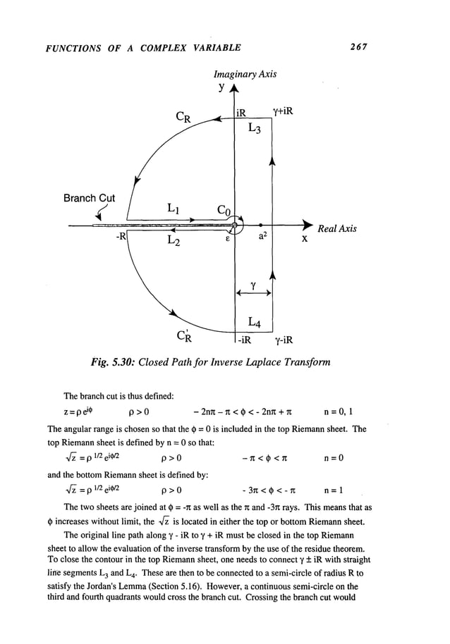
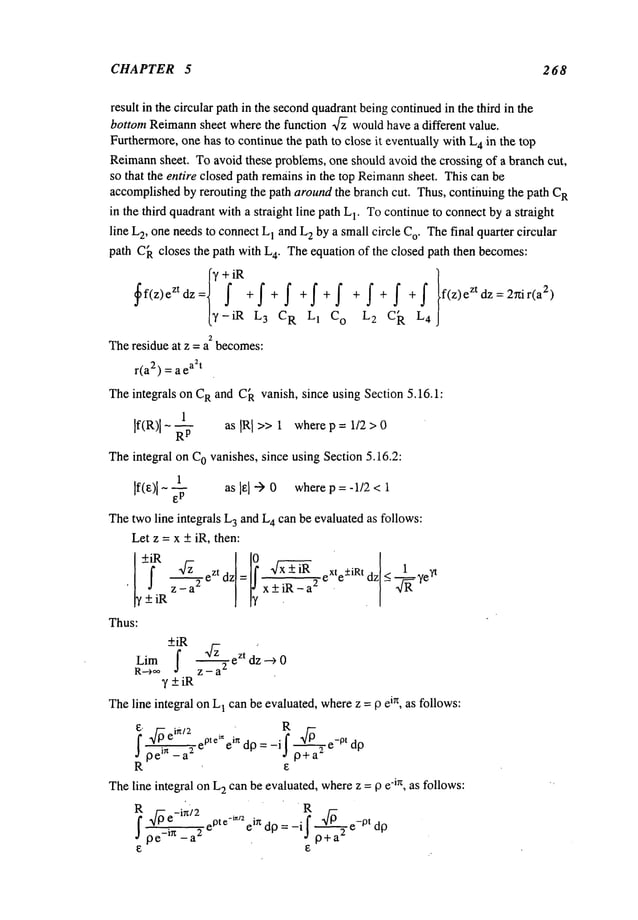
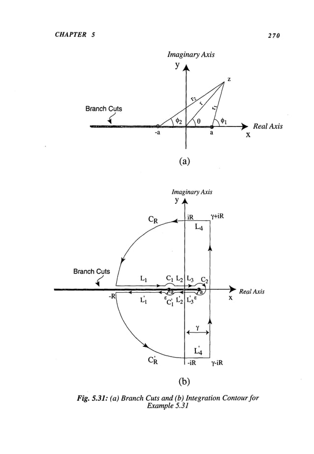
![FUNCTIONS OF A COMPLEX VARIABLE 271
z-a=rl
ei~t, -~Z<Ol <~, rl>0
z+a=r2
ei~2
, -71; < (~2 < ’/1; , r2>0
Thesingle-valuedfunction z is describedby:
z =r e
i0, r > 0
Theclosure of the original path from3’ - iR to 3’ + iR in the top Reimann
sheet would
require first the joining of twostraight line segments
3’ +iR to + iR, see Figure5.31(b).
Twoquarter circular paths, C
Rand C~are required to avoid crossing both branchcuts.
Tocontinue the path closure in the top Reimann
sheet, one has to encircle both branch
cuts. This takes the formof twostraight line path aboveand belowthe branch cuts from
C
Rand C~to the branchpoint at z = a. Since the straight line paths cross a singular
(branch)point at z = -a, then one mustavoidthat point by encircling it by twosmall
semi-circular paths C! and C~.Similarly, the joining of the straight line paths at the
branchpoint z = a requires the joining of the twoby a smallcircle C
2. Theline
segmentsbetweenz = -a and z = a is split into twoparts, namely,L
2 and L
3 and L[ and
L~. This is donepurely to simplify the integrations along these twoparts of each line
segment, as z on L
3 becomes-z along L
2. Theequation of the closed path becomes:
f
3’ + iR iR
~f(z)e zt dz= f + f + f
3’-iR 3’+iR C
R
a-£
0
onL
3
0
Ca a-E
onL~
+ f + f + f fz)eZtdz
-R c 1 -a-e
onL1 on L
2
-a+e -R )
+ ~ +I + ~ + ~ f(z)eZtdz=0
0 c i -a-e c~
onL~ onL
i
Theintegrals on C
Rand C~vanish as R"-> oo, since (Section 5.16.1):
1
If(R)l- ~- as R >> 1 where p = 1 > 0
Theintegrals on[3’+ iR to + iR] vanish since:
e(x+iR)t
I
l!4(x +iR)~--a2 dx< ~e~,t-->0 as R -->
Theintegrals on C
1, C
2 and C~vanish, since (Section 5.16.2):
z~a
Lim -- --> 0
z-~_+a~z2 _ a
2
Tofacilitate accountingof the integrandof these multi-valuedfunctions, onecan evaluate
the integrand term-by-termin tabular form. Thus, the remainingintegrals can be
evaluated in tabular form(see accompanying
table):](https://image.slidesharecdn.com/advancedmathematicalmethodsinscienceandengineering-hayek-230318001731-2b30ece5/85/advanced-mathematical-methods-in-science-and-engineering-hayek-pdf-285-638.jpg)
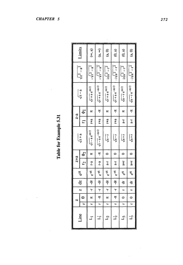
![FUNCTIONS OF A COMPLEX VARIABLE 273
Thesumof branchcut integrals L
1 + L~vanishes. This reinforces the stipulation
that running overlappingbranch cuts maymakethe function single-valued over the
overlappingsection. Thesumof the integrals over the branch cut integrals L
2 + L~, and
L3 + L~ become:
a a
I =-2il ert dr I =-2il e-rt’--dr
L2 + L2 0 ~a2 - r2
’ L3+L 0
Thefinal result for the inverse Laplacetransform:
f(t)
+
I ezt dz -1
2ir~ ¯ 2+L
2
e-rt dr 1 e-rt dr = i0(at)
whereI0 (at) is the Modified
BesselFunctionof the first kindandorder zero.
Example 5.32
Obtainthe inverse Laplacetransformof the followingfunction:
(z 2 _a
2)
f(z) : log/---~---
)
Theinverse Laplacetransformis definedas:
1 y+io~ 2 2
7 +i~
1
~ ~ [l°g(z-~)+l°g(z+a)-21°gz]
ez td z
Theintegrand is multi-valued, thus colinear branchcuts sta~ing fromthe branchpoints at
+a, 0, -a to -~ must be madeto makethe log~thmic functions single-valued, as shown
in Ng. 5.32(a). Thethree branch cuts de~nedfor the top Riemann
sheet of each of the
three logarithmicfunctionsare:
z-a= rl
ei0’, -~ < ~1 <g
z = r2 e
i02
, -/~ < 02 </~
z + a = r 3 e
i03
, -Tz < (~3 < ~
Thesingle-valuedfunction z is definedas:
z = r e
i0, r > 0](https://image.slidesharecdn.com/advancedmathematicalmethodsinscienceandengineering-hayek-230318001731-2b30ece5/85/advanced-mathematical-methods-in-science-and-engineering-hayek-pdf-287-638.jpg)
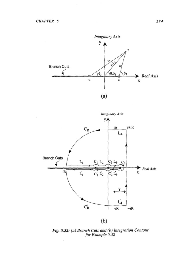
![FUNCTIONS OF A COMPLEX VARIABLE 275
Again,the branch cuts are chosento be colinear and overlappingextending fromx = a, 0
and-a to _oo.
Thecontour is closed on the complexplane as shownin Fig. 5.32(b). Thecontour
is wrapped
aroundthe three branchcuts, with small circular paths near each branchpoint
in such a wayas to leave the entire path in the top Riemann
sheet of all three logarithmic
functions. Thus,since there are no poles in the complex
plane, the closed path integral
is:
’I ¯¯ I
ff(z) zt dz
~’-iR ~’+iR C
R -R
on L
1
[c~2
a-e 0
+ +f +I+f +
E C~ a-E
on L
3 on L~
ICY i -R
y - iR
+
-a-E Ck -iR
on L~
--E
C1 -a-E
on L
2
-a+E t
f + f f(z)e
zt
c[
on L~
f(z)e zt dz= 0
Theintegrals on CR and C~vanish since:
log( R2. -a 2/
R
2 )I-RL~]I°g(1-~2)I
---a’~-~-Rp
Theintegrals on C1, C2, Ca, C~and C~vanish, since:
~- (’z
2
Lim/(z :1: a) 1og/------:l-//~
z-,_+a~_ ~. z
~
Lim[- (z2 _a2"~’l
Theintegrals on D’-+ iR to +_iR] vanishsince, on the line paths:
LimIf(z)l-~ a2
R---~,~ ~-T--~ 0 as R-) ~°
Theline integrals can be evaluatedin tabular formwhere:
(z2 _a:~
f(z) = log |----5~] =log (z - a) ÷log (z ÷ a)- 2 log
z- fl
dz
where p = 2 > 0](https://image.slidesharecdn.com/advancedmathematicalmethodsinscienceandengineering-hayek-230318001731-2b30ece5/85/advanced-mathematical-methods-in-science-and-engineering-hayek-pdf-289-638.jpg)
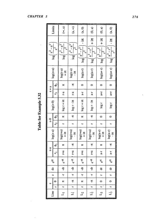
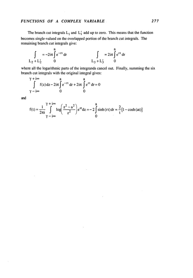
![CHAPTER 5 280
16. Findall the roots of:
(a) cos z =
(c) sin z = cosh a, ~ = real constant
(b) sin z =
(d) sinhz =
(e) eZ=-2 (f) log z =n
Section 5.4
17. Evaluatethe followingintegrals:
i
(a) J (z- dz
1
l+i
(b) j- (z - 1) on a parabola y = x
2
.
0
l+i
(c) ~ 3(x ~ +iy)dz
0
fz+2
(d) a 2z
C
(e) J" sin dz
C
ona straight line from1 to i.
on the paths y = x and y = x
3.
where
Cis a circle, ]z] = 2 in the positive direction.
whereCis a rectangle, withcorners: 0z/2,-g/2,n/2+i,-rt/2+i)
Section 5.5
18. Determinethe region of analyticity of the followingfunctions and showthat:
ff(z)dz =
C
wherethe closedcontourCis the circle Izl = 2.
z
2
(a) f(z) (b) f(z) =z
z-4
i
(c) f(z) = z2 (d) f(z) =tan (z/2)
sin z cos z
(e) f(z)=--- (f) f(z)=---
z z+3](https://image.slidesharecdn.com/advancedmathematicalmethodsinscienceandengineering-hayek-230318001731-2b30ece5/85/advanced-mathematical-methods-in-science-and-engineering-hayek-pdf-294-638.jpg)
![FUNCTIONS OF A COMPLEX VARIABLE 281
19. Evaluatethe followingintegrals:
i/2 l+i
(a) f sin(2z)dz (b) f (z2+l)dz
0 1-i
3+i
f Z2 dz (d)
(c)
0
j cosh z dz (f)
(e)
0
l+i
f
z2dz
0
i
fez dz
-i
20. UseCauchy’sIntegral formulato evaluate the followingintegrals on the closed
contourCin the positive sense:
~z
3 +3z+2 dz,
(a) Cis a unit circle [z[ = 1.
z
C
(b) f c°Szdz,
z
C
Cis a unitcircle [z[ =1.
(c) cos z dz
~c(Z_ ~)2
Cis a circle Izl
= 4.
f sin z dz
(d) ~C
(z - --~-~-’ Cis a circle Izl =4.
~[ 1 + 3 ,]dz
Cis acircle Izl=
3.
(e)
~ z+2
C
f Cis a ]z]=3.
dz
(f) 4 - 1’ circle
C
f
eZ+l
(g) -- dz, C is a circle Izl = 2.
z-ir~/2
c
(h) f tanz dz,
J z
2
C
Cis a unitcircle Iz[ =1.
Section 5.8
21. ObtainTaylor’s series expansionof the followingfunctions about the specified point
zo and give the region of convergence:](https://image.slidesharecdn.com/advancedmathematicalmethodsinscienceandengineering-hayek-230318001731-2b30ece5/85/advanced-mathematical-methods-in-science-and-engineering-hayek-pdf-295-638.jpg)
![FUNCTIONS OF A COMPLEX VARIABLE 283
z z3 - 4 z2 - 4
(d) sinz (e) 2+1)2 (f) z5_z3
z+2 1 1 Z
3
(g) z2(Z_2 ) (h) sinz-z (i) eZ-1 (j)
Section 5.11
25. Findthe residue of the function in problem
24 at all the singularities of each
function.
Section 5.12
26. Evaluatethe followingintegrals, wheren is an integer, and la] <1.
2n 2~
dO -
(a)
fl+2acos0+a
2sin(n0) dO
(b) f l_2asi---~0+£
2
0 0
27~
(c)-
cos3 0
dO (d)
1-2acos0+a
2 I(1 + a cos 0)
2
0
2n
cos(nO)
(e) I(sin0)2nd0 (f) I l+2acos0+a
2
0 0
i (sinO)2 (h) I(cosO)2ndO
(g) 1 + a cos
0 0
2rt
I" 1 +cos 0
;~cos2-----
~dO
(J) co s(nO) dO
(i) J cosh a + cos 0
0 0
n 2n
I dO
(1) I
(k) 1 + a cos
1 +a sin 0
0 0
r~
cos(20) dO
dO (n) Ii_2acos0+a
2
(m)
I (l+asinO)
~
0 0
Section 5.13
27. Evaluatethe followingintegrals, with a > 0, and b > 0, unless otherwisestated:](https://image.slidesharecdn.com/advancedmathematicalmethodsinscienceandengineering-hayek-230318001731-2b30ece5/85/advanced-mathematical-methods-in-science-and-engineering-hayek-pdf-297-638.jpg)
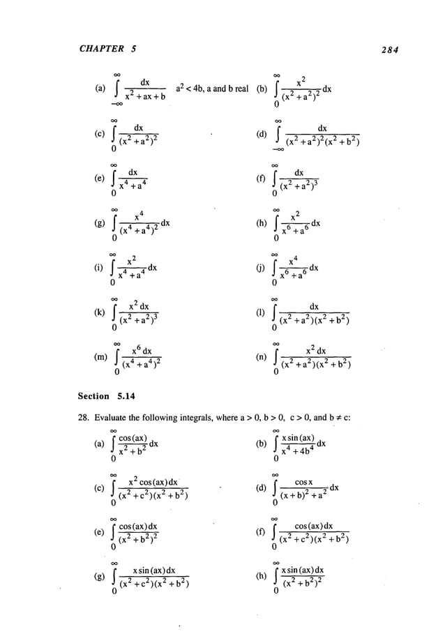
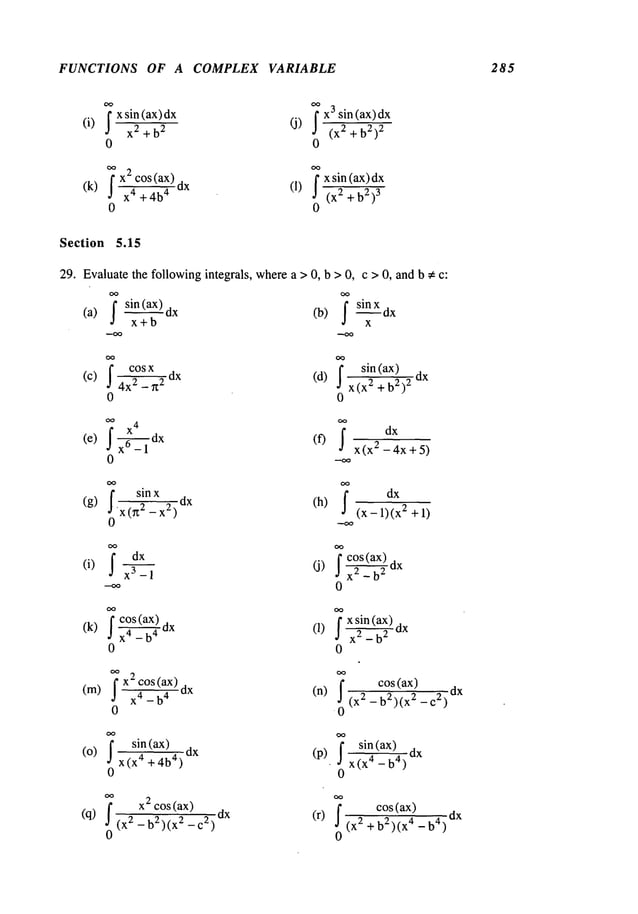
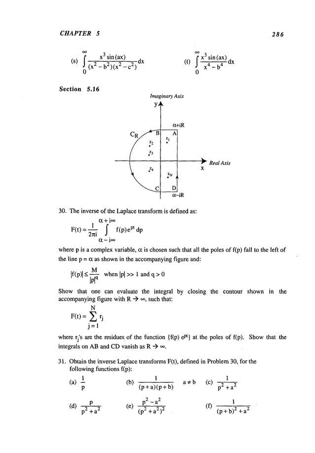
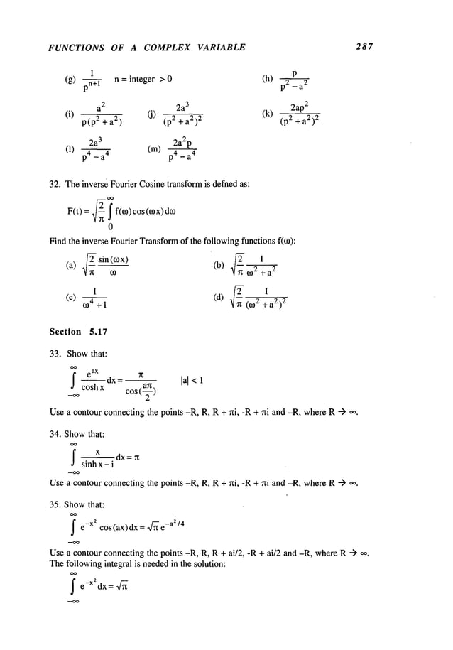
![CHAPTER 5 288
ImaginaryAxis
y~
R
Real Axis
36. Showthat:
OO
fcos(ax2)dx =
0
closethe contourbya ray, z =9 eirt/4, anda circular sector, z = Rei0, R-) oo,and
0 < 0 < r~/4, see accompanying
figure.
37. Showthat:
~ sinh(ax) dx= ltan (~) ]a]<l
sinh x
Usea contour connecting the points -R, R, R+ ~ti, -R + ni and -R, whereR-->
Section 5.18
38. Evaluatethe followingintegrals, wheren is an integer, with a > 0, b > 0 and a * b:
(l°gx)~ dx (b) f (1°~gx)~ dx
(a) 2 + 1) 2 xz + 1
0 0
f (1OgX)
2 dx
(c) ~(l°~gx,+lX)
4dx (d) a ~+1
0 0
X4 + 10X (X2 + 1)
2
0 0
~ (l-x2)logxdx (h)
1ogx
(g) 2 + 1) 2
(x2 + a2)(x2 + b
2)
0 0
dx
log x dx (j)
(i) f 2 + 1)4
0
f(l~x)z dx
xzn + 1
0](https://image.slidesharecdn.com/advancedmathematicalmethodsinscienceandengineering-hayek-230318001731-2b30ece5/85/advanced-mathematical-methods-in-science-and-engineering-hayek-pdf-302-638.jpg)
![FUNCTIONS OF A COMPLEX VARIABLE 291
1
(e)
z(~H
+a)
e-aZ
(g)
z+b
z
(m)
(z +b)
3/2
1
(o) 2 + a2
(s) (l°g z)2
z
1
(w)
~/(z +2a)(z +
(y) 2 +a2)
-v-l /2
(aa)
z(qT+a)
a
(CC) ff~(~f~+ b)(z_a2)
10 (z2 +a2"~
(ee) g~)
e_4"-~
~
(gg) 4~-
v > -1/2
1
(f)
(z +a)
b
e
a2/z
(h)
(j) log( z+ b
/
z+a]
(~z
z + a)2 +c
2
(1) log
+ b)2 + c
2
1
(n) ~zz
~/z + ~z2 +a
2
(P) 2 + a2
e-4-~
(r)
z
1
(v)
(z - a2)(ff~ +
1
(x) ~/(z + a)(z 3
1
(bb)
(z + a)
(dd)
(ff) e-4-~
(hh) arctan (a/z)
V>-I
b>a](https://image.slidesharecdn.com/advancedmathematicalmethodsinscienceandengineering-hayek-230318001731-2b30ece5/85/advanced-mathematical-methods-in-science-and-engineering-hayek-pdf-305-638.jpg)
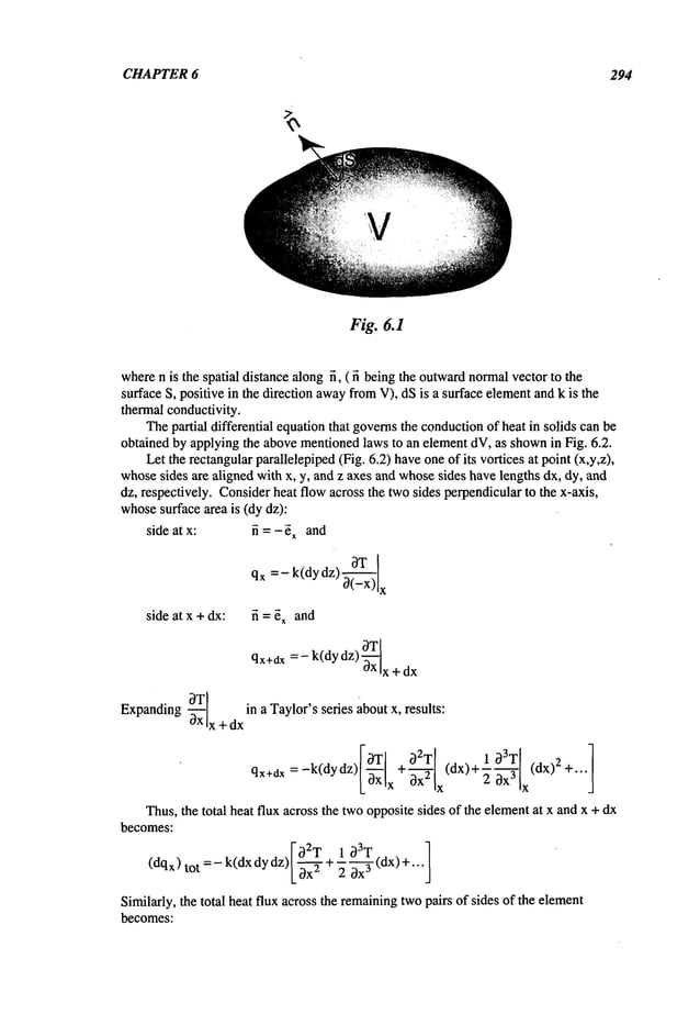
![PARTIAL DIFF. EQ. OF MATHEMATICALPHYSICS
qy+dy
295
qy
Fig. 6.2
and
tot L~z ~- ~-~-(dz) +...
Thus,the total heat flux into the element,to a first order approximation,
becomes:
02T 02T
dq:- k(dx dy dz) ( ~-~-~- +0-~+02T]
Thetime rate of changeof heat content of the elementbecomes:
dq = -c (p dx dy dz) 5
ot
If heat is beinggeneratedinside the elementat the rate of Q(×,y,z,t) per unit volume
then
the equation that governsheat flow in solids becomes:
0T k(02T+02T 02T’/
pc-~-=(,b--~-
3-~+3-~’J
+Q(x’y’z’t)
and the temperatureat any point P = P(x,y,z) obeysthe equation:
VZT
= 10T_ q(p, t) e in v t >0 (6.1)
K0t
wherethe material conductivity, K,is defined as K= k/pc, q is the rate of heat generated
divided by thermalconductivity k per unit volume,q = Q/k, and the Laplacianoperator
V
2 is definedas:](https://image.slidesharecdn.com/advancedmathematicalmethodsinscienceandengineering-hayek-230318001731-2b30ece5/85/advanced-mathematical-methods-in-science-and-engineering-hayek-pdf-308-638.jpg)
![CHAPTER6 296
Thesignof q indicates a heat sourceif positive, a heat sinkif negative.
Theboundary
condition that is required for a uniquesolution can be one of the
followingtypes: .
(a) Prescribe the temperatureonthe surface S."
T(P,0 = g(P,0 P on S
(b) Prescribethe heat flux across the surface
-k~-ffn (P,t)=/(P,t ) P on S
whereI is the prescribedheat flux into the volume
Vacross S. If l =0, the surface is
thermallyinsulated.
(c) Heat convection into an external unbounded
medium
of known
temperature:
If the temperaturein the exterior unbounded
region of the bodyis known
and equal to T
O
,
one maymakeuse of Newton’slaw of cooling:
8T
[T(P,t)- To(P, t)] P
-k-~-n(P, ) =
r
wherer is a constant, whichrelates the rate of heat convectionacross Sto the temperature
differential.
Thus, the boundarycondition becomes:
-~(P,t) + bT(P, t) = b To(P,t ) PonS where b=~
Thetype of initial conditionthat is required for uniquenesstakes the followingform:
T(P, +) =f(P) P in V
6.2.2 Diffusion of Gases
Theprocess of diffusion of one gas into another is describedby the following
equation:
1 ~C
V2C = ~ ~- q (6.2)
whereCrepresents the concentrationof the diffusing gas in the ambientgas, Drepresents
the diffusion constant andq represents the additional sourceof the gas beingdiffused. If
the diffusion process involvesthe diffusion of an unstable gas, whose
decomposition
is
proportional to the concentrationof the gas (equivalentto havingsinks of the diffusing
gas) then the processis definedbythe followingdifferential equation:
1~9C
V2C- ~tC = ~--~- - q ~t > 0 (6.3)
wherect represents the rate of decomposition
of the diffusing gas.
6.2.3 Diffusion and Absorption of Particles
Theprocess of diffusion of electrons in a gas or neutrons in matter canbe described
as a diffusion processwithabsorptionof the particles by matterproportionalto their](https://image.slidesharecdn.com/advancedmathematicalmethodsinscienceandengineering-hayek-230318001731-2b30ece5/85/advanced-mathematical-methods-in-science-and-engineering-hayek-pdf-309-638.jpg)
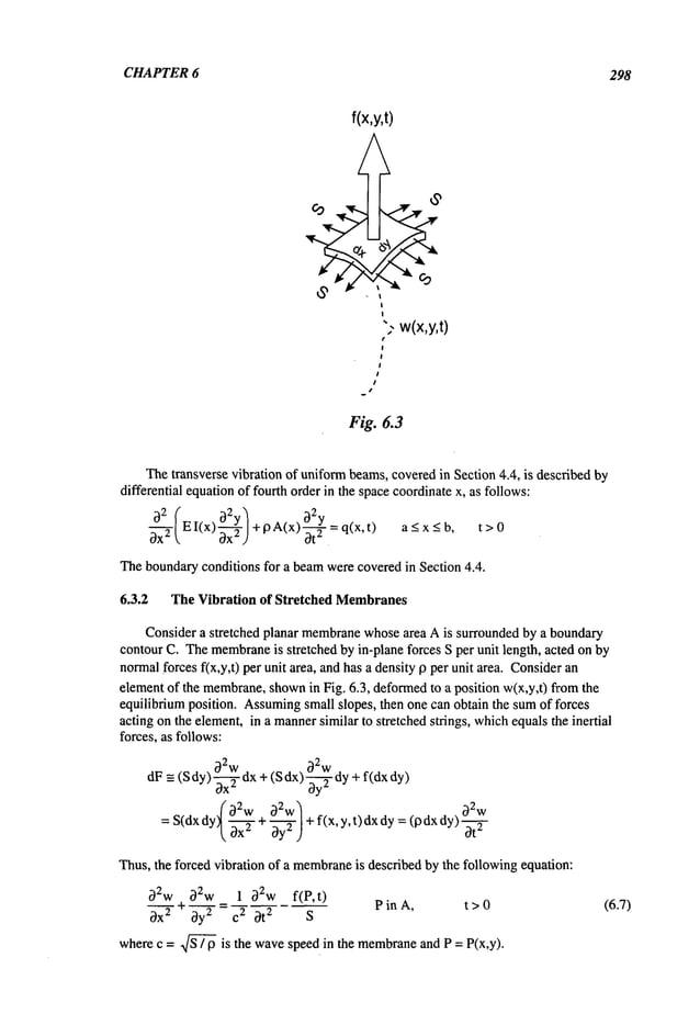
![CHAPTER 6 300
My
q(x,y,t)
dx
Vy
Fig. 6.4
V
x
i
x
c~2w
Mxy
=-D(1- v) 0x0"----~
where
D= plate stiffness ’-- Eh3/[120
- v2)].
The
shearforcescanberelatedto the derivativesof the moments,
such
that:
Vx=-D~xV2W and Vy=-D~yV2W (6.10)
Thefirst twoequilibriumeqs. of (6.8) are identically satisfied by expressionsfor the
moments
and shear forces given in equations (6.9) and (6.10). Substitution of the shear
forces of eqs. (6.9) and(6.10) into the third equationof (6.8) results in the equation
motionof plates on w(P,t):
DV4w
+ p h 0~--~ = q (P, t) Pin A, t >0 (6.11)
0t
whereV
4 = V2V
2 is called the BiLaplacian.
Theboundaryconditions on the contourboundaryC of the plate can be one of the
followingpairs:
(a) Fixed Boundary:Displacementw(P,t)
0w
Slope~-n (P,t) =0 PonC, t>0
(b) Simply Supported Boundary: Displacement w(P,t)
MomentM n- Do2wPt)=0 P C,t>0
- -
On
~( ,
on
(c) Free boundary: Moment
Mn= 0 [See item (b)]
V
n = -D-~ (P, t) = P on C, t >0
wheres is the distance measured
along C.](https://image.slidesharecdn.com/advancedmathematicalmethodsinscienceandengineering-hayek-230318001731-2b30ece5/85/advanced-mathematical-methods-in-science-and-engineering-hayek-pdf-313-638.jpg)
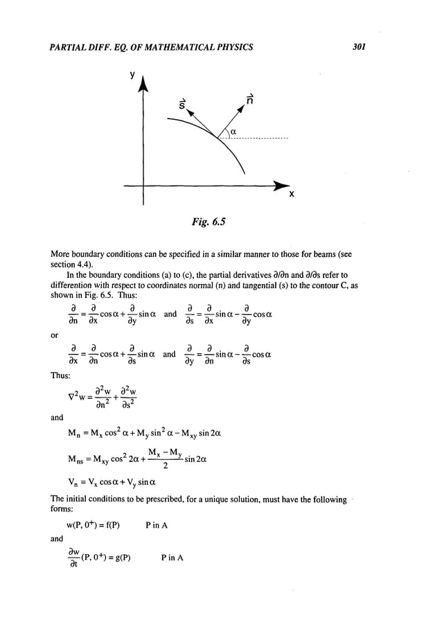
![CHAPTER 6 302
f(x+ct) f(x) f(x-ct)
ct ct
Fi£. 6.6
6.4 The Wave Equation
Thepropagation of a disturbance in a medium
is knownas wavepropagation. The
phenomena
of wavepropagationis best illustrated by propagationof a disturbance in an
infinite string.
Theequation of motionof a stretched string has the followingform:
~2y 1 ~)2y
OX
2 C2 0t
2
Thesolution of such an equation can be obtained in general by transformingthe
independentvariables x and t to u and v, whereu = x - ct and v = x + ct. Thus,the
equation of motiontransforms to:
~2y = 0
0u 0v
whichcanbe integrated directly, to give the followingsolution:
y = flu) + g(v)= f(x- ct) +g(x
Functionshavingthe formf(x - ct) and f(x + ct) can be shown
to indicate that a function
fix) is displacedto a position(ct) to the right andleft, respectively,as shown
in Fig. 6.6.
Thus,a disturbancehavingthe shapef(x) at t = 0, propagatesto the left and to the right
withouta changein shape, at a speedof c.
Aspecial formof wave
functions f(x +ct) that occurin physical applications is
knownas HarmonicPlane Waveshaving the form:
f(x + ct) = Cexp [ik(x + ct)] = Cexp [i(kx + tot)]
where
k = -- = wavenumber= --
c ~.
wavelength
to = circular frequency(rad/sec) = 2nf
f = frequencyin cycles per secondor Hertz (cps or Hz)
2~ 1
period in time for motion to repeat ....
C= amplitude of motion](https://image.slidesharecdn.com/advancedmathematicalmethodsinscienceandengineering-hayek-230318001731-2b30ece5/85/advanced-mathematical-methods-in-science-and-engineering-hayek-pdf-315-638.jpg)
![PARTIAL DIFF. EQ. OF MATHEMATICAL
PHYSICS 303
w(x,y,t)
undisturbed
__.__
surface
v(x,y,t)
~ u(x,y,t)
h
Fig. 6.7
6.4.1 WavePropagation in One-Dimensional Media
Theequationof motionfor vibrating stretched strings, bars, torsional rods, acoustic
horns,etc., togetherwiththe boundary
conditionsat the endpoints (if any)andthe initial
conditions makeup the wavepropagation systemfor those media.
6.4.2 WavePropagation in Two-Dimensional Media
Wave
propagation in stretched membranes
and in the water surface of basins make
up fewof the phenomena
of wavemotionin two dimensionalcontinua.
Thepropagationof wavesin a stretched membrane
obey the samedifferential
equation as the vibration of membranes,
with the sametype of boundaryand initial
conditions. Thesystemof differential equations, boundary
and initial conditionsare the
sameas those for the vibration problem.
6.4.3 WavePropagation in Surface of WaterBasin
Thepropagationof waveson the surface of a water basin can be developedby the
use of the hydrodynamic
equations of equilibriumof an incompressiblefluid. Let a free
surface basin of a liquid (A) (Fig. 6.7) be surrounded
by a rigid wall described
contourboundaryC, whoseundisturbedheight is h and whosedensity is 19.
Let u(x,y,t) andv(x,y,t) represent the components
of the vector particle velocity
fluid onthe surfacein the x andy directions, respectively,andw(x,y,t) be the vertical
displacement
fromthe level h of the particle in the z-direction.
Thelaw of conservationof massfor an incompressiblefluid requires that the rate of
changeof massof a columnhavinga volume
(h dx dy) mustbe zero, thus:
dX~x(uhdy) + dy~y (vhdx) + ~tt [(w + h)dxdy]](https://image.slidesharecdn.com/advancedmathematicalmethodsinscienceandengineering-hayek-230318001731-2b30ece5/85/advanced-mathematical-methods-in-science-and-engineering-hayek-pdf-316-638.jpg)
![PARTIAL DIFF. EQ. OF MATHEMATICAL
PHYSICS 305
V
p
as the rate of changeof massof an elementis zero. Thus,the increase in the massof the
elementmustbe equalto the influx of massthroughthe six sides of the element.Let u, v,
andwrepresentthe particle velocityof the fluid in the x, y andz directions, respectively.
Thus,the influx of massfromthe elementthroughthe twosides perpendicularto the
x-axis becomes:
9 u(x, y, z) dydx- 19u(x+dx,y, z) dydx=- 19u dx
dy dz
Similarly, the massinflux fromthe remainingtwopairs of sides becomes:
bv Ow
-p~y-ydxdydz and -p--~--xdxdydz
Thus,the law of conservationof massof a compressiblefluid elementrequires that:
~(pdxdydz) (~u ~v ~w~
~t = - P~xx+ -b--~y + "-~’z )
dxd
ydz
30 (Ou ~v Ow~:o
or
(6.17)
Let p(x,y,z,t) be the fluid pressureacting normal
to the six faces of the fluid element.
Theequations of motionof the elementcan be written as three equations governingthe
motionin the x, y, andz directions in termsof the fluid pressurep, bysatisfying
Newton’ssecond law:
x: [p(x,y,z,t) - p(x + dx,y,z,t)] dydz + fx Pdxdydz =(p dxdydz)
~t
y: [p(x,y,z,t) - p(x,y+dy,z,t)] dxdz+ fy p dxdydz =(p dxdydz)
~t
z: [p(x,y,z,t) - p(x,y,z +dz,t)] dxdy + fz P dxdy dz = (p dx dydz)
dt](https://image.slidesharecdn.com/advancedmathematicalmethodsinscienceandengineering-hayek-230318001731-2b30ece5/85/advanced-mathematical-methods-in-science-and-engineering-hayek-pdf-318-638.jpg)
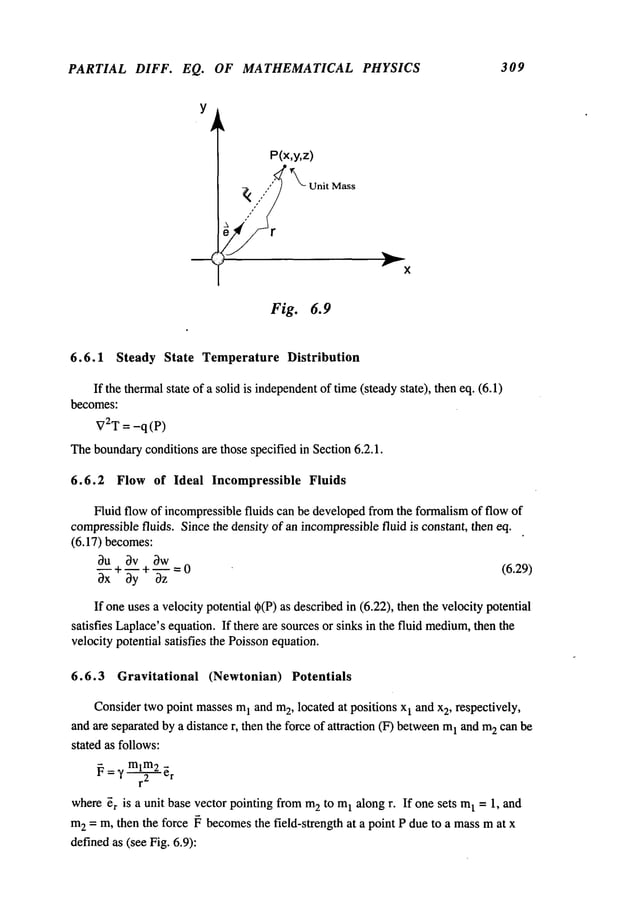
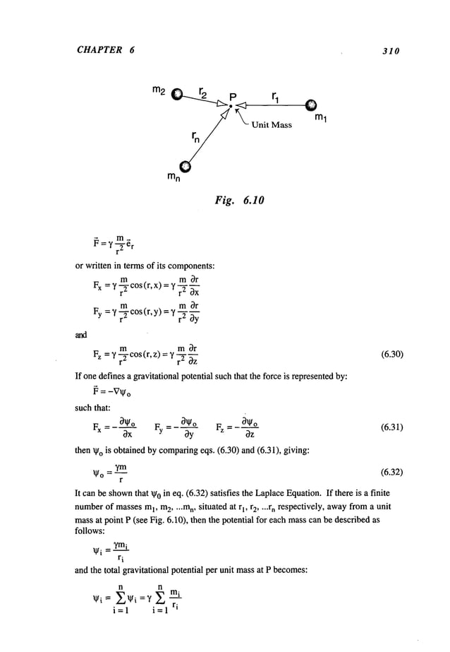
![PARTIAL DIFF. EQ. OF MATHEMATICAL PHYSICS 311
Z ~ ¯ P(x,y,z)
Y
X
If the massesare distributed in a volume
V, then the total potential dueto the mass
occupyingV becomes(see Fig. 6.11):
¯ =Y p(x ,y,z dV’ (6.33)
V
wherep(x,y,z) is the massdensity of the material occupyingVand ~ satisfies the
Poisson equation.
6.6.4 Electrostatic Potential
Theelectrostatic potential canbe definedin a similar mannerto gravitational
potential. Definethe repulsive (attractive) force F betweentwosimilar (dissimilar)
chargesof magnitudes
ql and q2, located at positions x1 and x
2, respectively, as:
~=qlq____~2
~
4~er2 r
wherer is the distance between
ql andq2 and e is the material’s dielectric constant. Define
the electric field as the force ona unit charge(whereq2= 1) locatedat a point Pdue to
chargeq2= q as:
]~= q ~ ~r =- q’~-’v(lq
4her
~ 4he rJ
If wedefine an electrostatic potential, ~, such that ~ = -V~, then a solution for the
potentialis:
~=q-fi-r
If there exists distributed chargesin a volume
V, then the potential can be definedas:](https://image.slidesharecdn.com/advancedmathematicalmethodsinscienceandengineering-hayek-230318001731-2b30ece5/85/advanced-mathematical-methods-in-science-and-engineering-hayek-pdf-324-638.jpg)
![CHAPTER 6 312
Ip(x’,
dV’ (6.34)
y’,z
p
)
W= 4~te r
V
wherep(x,y,z) is the chargedensity in V. It can be shown
that ~ satisfies the Poisson
equation.
6.7 Classification of Partial Differential Equations
Partial differential equationsare classified on the formof the equationin two
dimensionalcoordinates. Let the equation havethe following general form:
820
2
)
2b(x,t) a2* + a 0 = f~_~_~,a0,0,x
’
a(x,t) ~ + Ox0t c(x,t) ~ ~. 0x -~-
then the equationcanbe classified into three categories:
(a) Hyperbolic:Ifb2 > ac everywhere
in Ix, t].
Examples:TheWaveand Vibration equations.
(b) Elliptic: If 2 <aceve
rywhere in[x,t].
Examples:Laplace and Helmholtzequations.
(c) Parabolic:If 2 =
aceverywhere [x,
t].
Examples:TheDiffusion equation.
Theboundaryconditions amclassified as follows:
(a) Dirichlet: Specify 0(P,t) = g(P) P on S, t >
0 0(P, t) =g(p)
P on S, t > 0
(b) Neumann: Specify
00(P’t) ~- k0(P,t) = ) PonS, k>0, t>0
(c) Robin: Specify
(6.35)
6.8 Uniqueness of Solutions
6.8.1 Laplace and Poisson Equations
Uniquenessof solutions of the Laplaceand Poisson Equations, requires the
specification of boundaryconditions. Toprove uniqueness, assumethat there are two
different solutions of the differential equation. Let 01 and02 be twodifferent solutions to
Poisson’s equation (6.27), for a bounded
region V with identical boundaryconditions.
Thus,each solution satisfies the samePoissonequation:
V201 = f(P) and V202 = f(P) P in V
suchthat the differencesolutionsatisfies:
V20 = 0 where 0 = 01 - 02](https://image.slidesharecdn.com/advancedmathematicalmethodsinscienceandengineering-hayek-230318001731-2b30ece5/85/advanced-mathematical-methods-in-science-and-engineering-hayek-pdf-325-638.jpg)
![PARTIAL DIFF. EQ. OF MATHEMATICAL PHYSICS 313
Multiplyingthe previous Laplaceequation on ~) by ~ and integrating over V, one obtains:
_-0
V V S
Thus,
~[(~x) +(~yy) +(~-~z)2]dV=~c~-n~dS
V s
Tosolve for the difference potential giventhe three boundary
conditionsdescribed above:
(a) Dirichlet: If the twosolutions satisfy the sameDirichlet boundaryconditions
then:
~I(P) = q~2(P)= P on S
then:
~(P) = 0 P on
and eq. (6.36) becomes:
(0~)2 + (~-~-~)2]dV
=
J [(tgx )2+ ~ oz
V
which
canbesatisfiedif andonlyif 3_~_~
=0._~_~=--0~
=0 or ~=C =constant.
However,
0x 0y 0z
since q~ is continuousin Vand on S, and since ~ is zero on the surface, then the constant
Cmust be zero. Thus, ~ must be zero throughout the volume, and, hence, the solution
is unique.
(b) Neumann:
If normalderivatives of the potentials satisfy the sameboundary
conditionon the surface, then:
0~l(P) - 0~2 (P) =
P on S
On On
Thus:
D0(P) 0 P onS
On
Therefore, the difference solution ~ =C= constant, and the twosolutions are uniqueto
within a constant.
(c) Robin:If the two solutions satisfy the sameRobinboundaryconditions then:
O#2(P)
OOl(P~) + k~l(p) = __ + kO2(p)
P on S, k > 0
On On
Therefore:
- k~(P) PonS, k>O
On
and eq. (6.36) canbe rewritten:](https://image.slidesharecdn.com/advancedmathematicalmethodsinscienceandengineering-hayek-230318001731-2b30ece5/85/advanced-mathematical-methods-in-science-and-engineering-hayek-pdf-326-638.jpg)
![CHAPTER 6 314
I[(~ )2 "0@~2~,: +(~~-~)2]dV=-Ik02dSoz
+[~S,,j (6.37)
V s
However,
since k is positive and ~2 is positive, both integrals of eq. (6.37) mustvanish,
resulting in 0 = constant in Vand 0 = 0 on S. Dueto the continuancyof 0 in V and on
S, then 0 is zero throughoutthe volume
and the solution is unique.
6.8.2 Helmholtz Equation
Helmholtzequation can be solved by eigenfunction expansions. Thus, the
eigenfunctions 0M(P)
satisfy:
V20M+ XM0
M = 0 (6.38)
and homogeneous
boundaryconditions of the type Dirichlet, Neumann
or Robin. The
capitalized indexMrepresents one, twoor three dimensionalintegers and ~’Mis the
correspondingeigenvalue.
Thesolution to the non-homogeneous
Helmholtzequation (6.24):
720 + ~,~ = F (P) P in
canbe written as a superpositionof the eigenfunctions(~M(P)"
Let 01 and 02 be twosolutions of Helmholtz
equation (6.24), i.e.:
V201 + X01 = F (P) and V2~)2 + X~2 = F
If weonceagain define 0 as 01 - ¢2, then 0 satisfies the homogeneous
Helmholtz
equation:
V20+ ~,0 = 0 (6.39)
Expanding
the solutions for ~l and 02 in a series of the eigenfunctions:
01 = 2aM 0M(P)
M
02 = ZbM 0M(P)
M
then the difference solution 0 is expressedby:
0 = ~(aM -bM)0M(P)
M
Substituting 0 into eq. (6.39), and using eq. (6.38) one obtains:
Z(aM- bM)(~" -~.M) 0M(P) = 0
M
which,for X~ XM
and after usingthe orthogonality condition(Section 6.11) results
aM= bM. Therefore, Helrnholtz equation has uniquesolutions for any of the three types](https://image.slidesharecdn.com/advancedmathematicalmethodsinscienceandengineering-hayek-230318001731-2b30ece5/85/advanced-mathematical-methods-in-science-and-engineering-hayek-pdf-327-638.jpg)
![PARTIAL DIFF. EQ. OF MATHEMATICAL PHYSICS 315
of boundaryconditions.
6.8.3 Diffusion Equation
Let ~l and ¢2 be twosolutions to the Diffusion Equation(6.1) that satisfy the same
boundary
conditions andinitial conditions as follows:
1
~72~)1 - ~ ~-~ ÷ f(P,t) P in V, t > 0
1
V2O2-K 0t ~ f(P’t)
PinV, t>0
~(P,0+) = ¢2(P,0+) = g(P) P in V
Letting~ =~1 - ~2 then the differencesolution O(P,t) satisfies:
V20= 1 0¢ PinV, t>0
K 0t
and
¢(P,0+) = 0 P in V
and one of the followingconditionsfor points P on S and for t > 0:
(a)
(b)
or
(c)
Dirichlet: ~ (P, t) =
Neumann:
0 O(P, t) =
On
PonS, t>0
PonS, t>0
Robin: 0¢(P,t) ÷ hO(P,t) whereh>0, PonS, t>0
Multiplying the homogeneous
diffusion equation on the difference solution ~ by ~ and
integrating over V, one obtains:
1 f~ 0~ 1 ~) f~2dV f0V2(~d
V
-~-jq~-~-dV ....
2K 0t
V V V
(V,)-(V0) dV + f, (6.40)
V S
For Difichlet and Neumann
boundaryconditions, ~e surface integral vanishes and eq.
(6.40) becomes:
1 0~*~dV+~[( )~+ +( )~]dV=0 (6.41)
2K 0t ~
V V
For Robinboundarycondition, eq. (6.40) becomes:
2KOtf,2dV+I[( )2+( )2+(~)2]dV+hf,2dS=0
(6.42)
oz
V V S](https://image.slidesharecdn.com/advancedmathematicalmethodsinscienceandengineering-hayek-230318001731-2b30ece5/85/advanced-mathematical-methods-in-science-and-engineering-hayek-pdf-328-638.jpg)
![CHAPTER 6 316
Foreither eq. (6.41) or (6.42) to be true:
~ttf~
2dv-<O
V
Let:
j" ~2dV
= F(t)
V
Since the time derivative is alwaysnegative, due to the inequality in eq. (6.43), wecan
definea newvariable, f(t), suchthat:.
~F(t) = _[f(t)]2
bt
t
F(t) = -f [f(n)] 2 drl + C
0
Since ~(P,0+) = 0, then F(0) = 0 and hence C= 0. Thus:
(6.43)
t
0 V
whichis only possible if integrandg) = 0. Therefore, the solution mustbe unique.
6.8.4 Wave Equation
Let ~1 and ~)2 be solutions to the Wave
Equation(6.23) whichsatisfy the same
boundary
conditionsand initial conditions, suchthat:
= 1 b2~+q(P,t). PinV, t>O
~72~1 c2 ~t
2
= 1 bZ~z ~-q(P,t) P in V, t > 0
V2~)2 2 ~t
2
~I(P,O+) = ~2(P,O
+) = f(P) P in V
-~tl(p,0+)=~-~L(P,0+)=g(P) PinY
for Pin Vandt > 0, suchthat the differencesolution @
satisfies:
1 ~)2~
PinV, t>O
V2~ = C2 ~t
2
~(P, +) =0 P in V](https://image.slidesharecdn.com/advancedmathematicalmethodsinscienceandengineering-hayek-230318001731-2b30ece5/85/advanced-mathematical-methods-in-science-and-engineering-hayek-pdf-329-638.jpg)
![CHAPTER 6 318
Remember,
that for the Dirichlet boundarycondition, @(P,t)= 0 for P on S and for
t > 0. Therefore,the time derivative of the boundaryconditionvanishes, i.e.:
-~(P, t) = 0 for P on
For Neumann
boundaryconditions:
0~-~(P,t) = 0 for Pon
Thus, for either Dirichlet or Neumann
boundaryconditions, the surface integral vanishes
and eq. (6.46) becomes:
+(~-z
(6.47)
Integrating eq. (6.47) wi~respect to t. oneobtains:
[ 1 (0,) 2 +(~0)2 +(00)2
]
~ +(~)~dV=C(constantforallt)
V
Substitutingt = 0 in the integrand,thensince$(P,0
+) = 0for Pin V, then
a~(~,o
+)
V@(P,O+)=O.
Also, since ~ =0forPin V, thenC=0in Vandtheintegrand
mustvanishfor all t. Thus:
aS_o, a~=o, ~$ a~=o, PinV, t>0
aS- #=o, aS
which,when
integratedresults in:
@(P,
t) = 1 =constant Pin V, t > 0
Since
$(P,0
+)= 0, thenC~
= 0and
@(P,t)
~ Pin V,t > 0
For Robinbounda~
condition, eq. (6.46) becomes:
+(~)Z + (0@)Z + (~)2]d
V
V
a@dS=h 3 f@2dS
(6.48)
-hf* 2at
S S
Integratingequation
(6.48)withrespectto t resultsin a constant:
/[~(~)2 +(0,)2~ +(~3,)2 +(~)2]dV+~f,2dS= Coz
V S
Invoking the same~gumentsas above, C= 0, and, one can again showthat:
~(P,t)~0 PinV, t>0
Therefore.all three bounda~
conditionsare sufficient to producea uniquesolution in
wavefunctions.](https://image.slidesharecdn.com/advancedmathematicalmethodsinscienceandengineering-hayek-230318001731-2b30ece5/85/advanced-mathematical-methods-in-science-and-engineering-hayek-pdf-331-638.jpg)
![CHAPTER 6 320
for a ¢ 0: X = A sinh (ax) + B cosh (ax)
Y = Csin (ay) + Dcos (ay)
for a =0: X=Ax+B
Y=Cy+D
Applyingthe boundaryconditions to the solution, and assuring non-trivial solutions, one
obtains:
T(x,0)=DX(x)=0 -)
T(x,H) = C sin (all) ¯ X(x) = sin (all) =
Tosatisfy the characteristic equation,sin (all) = 0, "a" musttake one of the following
characteristic values:
n~
a n = ~ n =1,2,3....
Thenon-trivial solution of Y(y)consists of an eigenfunctionset:
Cn(Y)= sin (nny/H)
wherethe eigenfunctionsCn(Y)
are orthogonalover [0,HI, i.e.:
H
f {0
nCm
sin(nny/H) sin(mny/H)dy = H / 2 n
0
Thea = 0 case results in a trivial solution. Substituting the solution into the second
boundarycondition:
T(L,y) = [Asinh (anL) + B cosh (anL)] Y(y)
whichcanbe satisfied if:
B/A= - tanh (anL)
Finally, the solution canbe written as:
n~
~nn cosh( -~ x)]
n =
Tn(x,y) = sin( y)[si nh ( - -ff x) - t anh(L) 1,2
Tn(x,y) satisfies the LaplaceEquationand three homogeneous
boundaryconditions.
Dueto the linearity of the system,one can use the principle of superposition, such that
the temperaturein the slab can be written in termsof an infinite GeneralizedFourier
series in termsof the solutions Tn(x,y),i.e.:
T(x,y) = n Tn(x,y)
n=l
Theremainingnon-homogeneous
boundarycondition can be satisfied by the total
solution T(x,y) as follows:
OO
T(0,y) = f(y)= n
tanh( -~-_n
L)sin(~-~n
n=l](https://image.slidesharecdn.com/advancedmathematicalmethodsinscienceandengineering-hayek-230318001731-2b30ece5/85/advanced-mathematical-methods-in-science-and-engineering-hayek-pdf-333-638.jpg)
![CHAPTER 6 324
If frO)is constant= o, then:
En=Fn=0 n= 1,2,3 ....
Eo
-- T
O
Thus,the temperaturein the annularsheet is constant and equals T
O
.
Example 6.3 Steady State Temperature
Distribution in a Solid Sphere
Obtainthe steady state temperaturedistribution in a solid sphereof radius = a, where
T = T(r,0), and has the temperaturespecified on its surface r =a as follows:
T(a,0) =f(0)
Examination
of the boundarycondition indicates that the temperaturedistribution in the
sphere is axisymmetric, i.e, 0/~ = 0. Thus, from AppendixC:
VET
rELo~rt.
-ff~-rJ+si-7"~-~’~’ts’nO-ff~’)]
:°
LetT(r,O)
=R(r)
U(O),
1 d r E dR 1
sin
R dr ~r Usin O -~-J
Since the non-homogeneous
boundarycondition is in the r-coordinate, then k2 > 0 results
in an eigenfunction in the 0 - coordinate. Thus, the twocomponents
satisfy the
following equations:
rER
" + 2rR’- k2R= 0
U" + (cot0) U’ + kEU=
Transforming
the independentvariable from0 to rl, such that:
vl =cos 0 -l<rl< 1
then Usatisfies the followingequation:
d---I(1- na)-~
}+kEu--0dn
Letting k2 = v (v + 1), where>0,then thesolution to t he diff erential equation
becomes:
U(rl) = v Pv(rl) + v Qv(
rl)
R(r) = rv + Dv
r-(v+l)
= Er-1/2 + Fr-1/2 log(r)
1
forv¢ --
2
1
for v=--
2](https://image.slidesharecdn.com/advancedmathematicalmethodsinscienceandengineering-hayek-230318001731-2b30ece5/85/advanced-mathematical-methods-in-science-and-engineering-hayek-pdf-337-638.jpg)
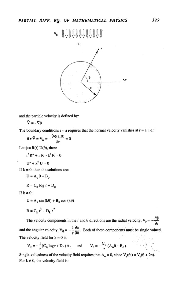
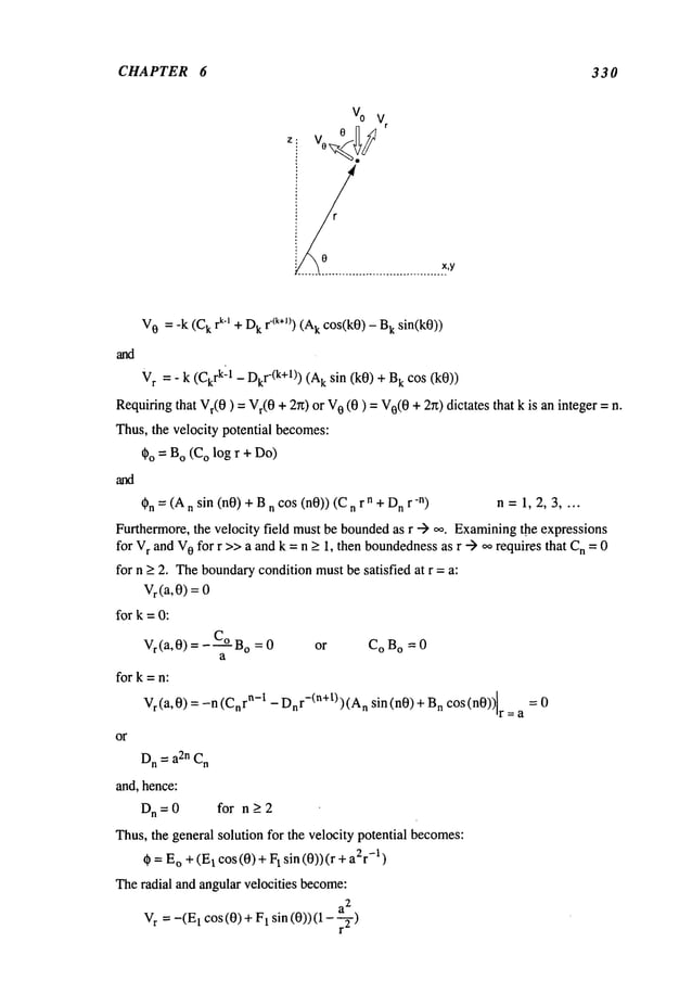
![PARTIAL DIFF. EQ. OF MATHEMATICAL PHYSICS 331
V
0 = +(E
1 COS(0)
- 1 sin (0)) ( 1 +
Theradial and angularvelocities mustapproachthe given velocity V
o in the far-field of
the cylinder,i.e.:
V
r ---) -V
o sin (0) and V
0 --) -V
o cos (0)
which, whencompared
to the expressions for V
r and V
O, gives:
E
1 = 0 and F1 = V
o
Thus,the solution for the velocity field takes the final form:
2
V
r =-V
o (1 - ar-~-) sin(O)
2
a
V
0 -- -V
o (1 ÷ 7) cos(0)
and
¢=Eo+vo(r+ - )sin(0)
r
Notethat the velocity potential is uniquewithin a constant, due to the Neumann
boundarycondition, and unbounded.However,
all the physical quantities (V
r and V
0) are
unique, single-valued and bounded.
Example 6.6 Electrostatic Field Withina Sphere
Obtainthe electric field strength produced
in twometal hemispheres,
radius r =a,
separatedby a narrowgap, the surface of the upperhalf has a constant potential ~o, the
surfaceof the lowerhalf is beingkept at zero potential, i.e.:
~(a’0)=f(0)={00°rt/2<0<r~0-<0<x/2
Since the sphere’s shapeand the boundary
condition are independentof the polar
angle, then the solutions can be assumed
to be independentof the polar angle, i.e.
axisymmetric.
Theequationsatisfied bythe electric potential (~ in spherical coordinates,
for axisymmetricdistribution, is given by (Appendix
C):
32t~ . 2 3¢ . 1 32¢ cot(0) 3¢
V2*= 3r’--~-*~--~-r*~-a-’~ -+ r 2 30
Let qb(r,0) = R(r) U(0), then the solution as given in Example
6.3 becomes:
Ck= [AkPk 0q) + BkQk(rl)] rk + D
kr-k-l]
whererI = cos 0
Boundedness
of the voltages E
r and E
0 at r = 0 and r1 = + 1 requires that k =integer =
n, B
n = 0 and D
n = 0. Thus,the solution whichsatisfies Laplace’sequation is:
t~n(r, rl) =nP
n (rl) n = 0, 1, 2 ....](https://image.slidesharecdn.com/advancedmathematicalmethodsinscienceandengineering-hayek-230318001731-2b30ece5/85/advanced-mathematical-methods-in-science-and-engineering-hayek-pdf-344-638.jpg)
![CHAPTER 6 332
andthe general solution canbe written as a GeneralizedFourier series:
~)= ~ Fn rn Pn(rl)
n=0
Satisfying the boundary
condition at r = a:
~(a, rl) = n rnPn(rl) = g (~
n=0
whereg (rl) = f (cos -1 rl). Thus,usingthe orthogonality of the eigenfunctionsPn0]),
results in the followingexpressionfor the Fourier coefficients:
+1 +1
Fn=
2n+~1.2a
nj-g(rl)pn(rl)dr
I =2~
-~°2n+l’
j’Pn(rl)dr
I
-i 0
Thefirst fewFourier constants become:
~a 7 11
F° : ~)~°2 FI= *o F3 = - 1-~a3 *o F5= 3-~-a5*o
F2n =0 n =1,2,3,4....
Therefore,the potential can be written as:
g)(r, rl)=-~ l+3(r)pl(rl)- ~ ; P3(rl)+ P5(rl)-...
2a) 16aJ
Theelectric field strength ~ = E
r ~r + E0~0
= ~7~)can be evaluatedas follows:
Er(r, rl)-~)* *o{~P10])_21(r~2p()+55(’r’)
4
10,. 0 o /-,’,’,’,’,’,’,’,’,~ ~ 3 .... 7(" r):~ p,. )+ ll[r) 4 }
6.10 The Poisson Equation
Solution of Poisson’s equation maybe obtained in terms of eigenfunctions. Two
distinct types of problemsinvolving Poisson’s equation will be discussed; those with
homogeneous
boundary conditions and those with non-homogeneous
ones.
In problems involving homogeneous
boundaryconditions, one mayattempt to
construct an orthogonaleigenfunctionset first, whichis then used to expandthe source
function in Poisson’s equation.
Start with the following system:
V2(~ = f(P) P in V (6.49)
together with homogeneous
boundaryconditions of the Dirichlet, Neumann
or Robin
type, written in general form:](https://image.slidesharecdn.com/advancedmathematicalmethodsinscienceandengineering-hayek-230318001731-2b30ece5/85/advanced-mathematical-methods-in-science-and-engineering-hayek-pdf-345-638.jpg)
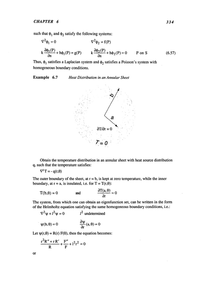
![CHAPTER 6 336
T(r,0)= Z Z Rnm(r)[
Anmsin(n 0) +Bnmc°s(n0)]
n=0m=l
Thesolution for the Fourier coefficients Anm
and Bnr
n can be obtained in the formgiven
in eq. (6.55), using the orthogonalityof Rnm
and the Fourier sine and cosine series as:
b2u
a
2
[ |rq(r,0)Rnm(r)sin(n0)d0dr n, m:= 1, 2, 3 ....
Anm - 2
~nm Nnm
d J
a0
b2u
a2en f f r q(r,0) Rnm(r) c°s(n0)
Bnm
2~2nrn Nnma 0
n=0,1,2 ....
m=1,2,3 ....
whereen is the Neumann
factor.
6.11 The Helmholtz Equation
The solution of homogeneous
and non-homogeneous
Helmholtzequation is outlined
in this section. Considerthe Helmholtzequation (6.24):
V2~)+)~ ~ =f(P) P in V (6.24)
subject to homogeneous
boundaryconditions (6.50):
U
i (~)(P)) P on S (6.50)
Thehomogeneous
eigenvalue systemgiven in eqs. (6.51) and (6.52) generate
eigenfunctionset that is orthogonalas defined in eq. (6.53). Theeigenfunctions~)M (P)
satisfy Helmholtz
equationwhen
)~= ~’M,i.e. (6.52)
V2~)M÷ ~M~M= f(P) (6.52)
Onecan showthat the eigenvalues are non-negative. Multiplying the Hel~olm
equation on ~Mby ~Mand integrating on V, one obtains:
I*M[V2*M+ ~M*M]
dV = -f (V*M)*(V*M)dV +
V V V
+f ~MO~MdS = 0
On
S
whichcan be rewritten as:
I ~V*M~ dV - XM I *~ dV = I*M ~ :0 (6.58)
V V S
Now
one can solve for XM
for the given bounda~condition:](https://image.slidesharecdn.com/advancedmathematicalmethodsinscienceandengineering-hayek-230318001731-2b30ece5/85/advanced-mathematical-methods-in-science-and-engineering-hayek-pdf-349-638.jpg)
![PARTIAL DIFF. EQ. OF MATHEMATICAL PHYSICS 337
(a) Dirichlet: ~)M (P) = 0 P on S, then:
IV,MI
=dV
~’M = V >0
V
(b) Neumann:O%I(P)
On
P on S, then:
(6.59)
the same~onclusionsabout ~’M in eq. (6.59) are made.
(c) Robin: 00M(P)
On ÷h0M(P) = 0 P on S and h > 0 then:
J’lV12dV
KM = V
S >0 (6.60)
V
Thus, the eigenvalues correspondingto these boundaryconditions are real and non-
negative.
Onecan showthat the eigenfunctions are also orthogonal. Let ~ and ~Kbe two
eigenfunctionssatisfying eq. (6.38) correspondingto eigenvalues~’Mand ~K,with
~’M
~: )~K,i.e.:
V2¢M + ~’M~M = 0
(6.60
V2¢K
+ XKCK
= 0
Multiplyingthe first equation in (6.61) by ¢K,and the secondin (6.61) by
subWacting
the resulting equalities and inte~ating over V, one obtains:
yi*KV~*~
- ¢~V2*¢laV
+ ~XM
- XK)y*~¢K
dV ~6.62~
V V
Fromvector calculus, it can be shown
that:
f fV2gdV=- I(Vg)*(Vg)dV+I
V V S
Thus, eq. (6.62) becomes:
~3~M ~]dS XM)
y 0M#KdV (6.63)
S V
If the eigenfunctions ~Kand @M
satisfy one of the bound~
conditions [eq. (6.50)], then
the left side of eq. (6.63) vanishesresulting in:
y@M
dV 0 M K
~K
V](https://image.slidesharecdn.com/advancedmathematicalmethodsinscienceandengineering-hayek-230318001731-2b30ece5/85/advanced-mathematical-methods-in-science-and-engineering-hayek-pdf-350-638.jpg)
![CHAPTER 6 340
then the Fourier coefficients Enm
of the doubleFourier series can be obtainedfromeq.
(6.65) in an integral form:
LL
-4 )
Enm= L
2 (k2 ~ I I q° sin( nrtx/sin( mrt y dx dy
-knm)o 0 S t~ L J
-16 qo
mnx2(k 2 2
-knm) S
if mand n are both odd
= 0 if either mor n is even
Finally, the response of the membrane
to a uniformdynamicload is:
oo oo sin(~ x) sin(~-~
w(x’y’t)=-16q° " " "Z
_k2mn)
n2"----
~ sin(COt) mn (k
2
n=lm=l
for m, n odd
Example 6.9 FreeVibrationof a CircularPlate
Obtainthe axisymmetric
mode
shapes and natural frequencies of a free, vibrating
plate, havinga radius = a, and whoseperimeteris fixed. Let the displacementof the plate
wbe written as follows:
w(r,t) =W(r)i°~t
then the equation of motionsatisfied by W(see equation 6.11) becomes:
-V4W+ k4W = 0 k4 = 0ho~2
D
Theequation can be separated as follows:
(V2 - k2)(V2 + k2)W=
whosesolution can be sought to the following equations for k # 0:
(V2 +k2)W = W= AJo(kr) + BYo(kr).
(V2 - k2)w = 0 W= CIo (kr) + Do (kr)
whereJo and Yoare Besselfunctions of first and secondkind andIo and K
o are modified
Besselfunctionsof the first andsecondkind respectively, all of themare of order zero.
Boundedness
of the solution at r = 0 requires that B= D=0, so the total solution can
be written as follows:
W(r)= AJo(kr) + o (kr
For a fixed plate the boundaryconditions are w= 0 and Ow/~r= 0 = 0 at r = a, and are
satisfied by:
w(a) = A Jo(ka) + o (ka) = 0
OW
~- (a) = k[A Jg(ka)+CI~(ka)]
which,gives the characteristic equation:](https://image.slidesharecdn.com/advancedmathematicalmethodsinscienceandengineering-hayek-230318001731-2b30ece5/85/advanced-mathematical-methods-in-science-and-engineering-hayek-pdf-353-638.jpg)
![PARTIAL DIFF. EQ. OF MATHEMATICAL PHYSICS 341
Jo(ka)I~(ka)- Io(ka)J~(ka) = 0
Let the roots t~n, where
tx =ka, of the characteristic equationbe designatedas:
ct
n=kna n=1,2,3 ....
whereit can be shown
that there is no zero root. Theeigenvalues are X
n = k4n= Ct4n/a4.
Theeigenfunctionscanbe evaluatedby finding the ratio C/A= -Jo(Ctn)/Io(Otn)
substituting that ratio into the solution. SinceJo(Ctn)~: 0, then onemay
factor it out.
Thus, the natural frequencies (on and the mode
shapesW
n are then foundto be:
(on
~ oh a
2
n=1,2,3 ....
jo(ctnr) io(~nr)
Wn_ a
a
Jo(Rn) Io(t~n)
Example 6.10 FreeVibration of GasInside a Rigid Spherical Enclosure
Obtainthe mode
shapes and the correspondingnatural frequencies of a gas vibrating
inside a rigid spherical enclosurewhose
radius is a.
Thevelocity potential ~(r,0,~,t) of a vibrating gas inside a rigid sphereis assumed
have harmonictime dependence,such that:
w(r,0,~,t) =W(r,0,q~)
i(Ot
whereWsatisfies the Helrnholtz equation. Assuming
that Wcan be written as:
W(r,0,~) = R(r) S(0)
then the Helmholtzequation becomes:
R" 2R’ I[’S" S’~ 1 M"
--+---+
+cos0~-j+
~k
2=0
R r R r
2L ~- r 2sin20 M
whichseparatesinto three ordinarydifferential equations:
r2R"+ 2r R’ + [k2r2 - v (v +1)] R=
M" + ~2M= 0
~2
S"+ cot 0 S’ +[v (v + 1)- si---~] S=
the last of whichtransformsto the followingequationif onesubstitutes rl = cos 0:
d_~[(l_ r12) d~] + [v(v + 1)_
~_--~]s =0
Theseparation constants v and ct2 mustbe positive or zreo to give oscillating solutions
of the three ordinarydifferential equations. Thesolution of these equationscanbe written
as follows:](https://image.slidesharecdn.com/advancedmathematicalmethodsinscienceandengineering-hayek-230318001731-2b30ece5/85/advanced-mathematical-methods-in-science-and-engineering-hayek-pdf-354-638.jpg)
![CHAPTER 6 342
R = Ajv(kr)+ BYv(kr)
S = CP~Oq)
+ DQv~(rl)
M= Esin(et0) +
whereJv and Yvare the spherical Bessel Functionsof the first and second~ndof order v,
P~ and Q~~e the associated Legendrefunctions of the first and second~nd, degree v
and order ~. Single-valuednessrequires that ~ be an integer = m= 0, 1, 2 .... and
~undedness
at r =0 and ~ = ~ 1 requires that:
B = D = 0 ~d v is an integer =n =0, 1, 2 ....
Thebounda~
condition at r = a requires that the nodal (radial) velocity mustvanish,
i.e.:
V
r = - ~ = 0 or j~ (ka) = j~ (~) where ~ = ka
r a
Let ~nl designatethe 1 t~ root of the n" equation. It can be shown
that the roots ~nl ¢ O.
Themode
shapesand natural frequenciesof a vibrating gas inside a spherical enclosure
~come:
a LCOS(n0)J
C
¢0nl=-- ].tnl re, n=0, 1,2,3 .... / =1,2,3 ....
a
6.12 The Diffusion Equation
Themost general systemgovernedby the diffusion equation takes the form of a non-
homogeneous
partial differential equation, boundaryand initial conditions, havingthe
form
V2
~ = 1 30 + F(P, t) P in V, t > 0 (6.66)
K 3t
where~ = q~(P,t) is the dependentvariable satisfying time-independentnon-homogeneous
boundaryconditions of Dirichlet, Neumann
or Robintype, i.e., they are only spatially
dependent:
U(O(P,t)) = l P on S, t > 0 (6.67)
andthe initial conditions:
t~(P,0+) =g(P) P in V (6.68)
and F(P,t) is a timeand space dependentsource. Therestriction on only spatially
dependentboundaryconditions is due to the goal of obtaining solutions in terms of
eigenfunctionexpansions, such restrictions will be removedin Chapter7.
Since the non-homogeneous
boundaryconditions are only spatially dependent, one](https://image.slidesharecdn.com/advancedmathematicalmethodsinscienceandengineering-hayek-230318001731-2b30ece5/85/advanced-mathematical-methods-in-science-and-engineering-hayek-pdf-355-638.jpg)
![CHAPTER 6 344
which
uses eq. (6.72). Rearranging
eq. (6.74)results in a morecompact
form:
~ (EL(t) + ~’M
KM(t)) ~ = -KF(P
, t) (6.75)
M
Multiplying
eq. (6.75)by0N(P)
andintegratingoverthevolulneresults in a fixst order
ordinary
differential equation
onthetime-dependent
Fouriercoefficients:
~t~M(P) F(P, dV
t)
E~l(t) + ~M
KM(t) = -K
V = FM(t) (6.76)
V
Thesolutionof the non-homogeneous
first-order differential equation(6.76) is obtained
in the form,givenin Section1.2:
t
E
M(t) = C
Me-K~’Mt+ ~ F M(~I)e-~’uK(t-Vl)dl"l (6.77)
0
Onecanuse the initial conditionat t = 0 to determine
the unknown
constantsC
M
Ol (P, 0+) = ~ EM
(0) OM
= h(P)=~ C
M
~M
(P) (6.78)
M M
since EM(0
) = C
M.Thus,usingthe orthogonalityof the eigenfunctions,the constants
C
Mbecome:
CM= ~M! h(P)~M(P)dV (6.79)
Theevaluationof C
Mconcludes
the determination
of the Fouriercoefficients EM(t
). The
solutionin (6.77)is a linear combination
of twoparts, onedependant
onthe initial
condition,C
M,andthe other dependant
onthe sourcecomponent,
FM(t).If the heat
sourceis not timedependent,
i.e. if F(P,t) = Q(P)only, thenM=QM
, a co
nstant, and
the solutionfor EM(t)
simplifiesto:
EM(t) = CMe-K~,~tt + QM[1- e
-K~’ut
] (6.80)
~.M
K
andC
Mis definedbyeq. (6.79).
Example 6.11 HeatFlowin a Finite Thin Rod
Obtainthe heat flowin a finite rodof lengthL, whose
endsare keptat constant
temperature
a andb. Therodis heatedinitially to a temperature
f(x) andhasa distributed,
time-independent
heat source,Q(x),suchthat, for T= T(x,t):
02T 1 0T Q(x)
0-~ "= K Ot Kpc
T(0,t) =a = constant T(L,t)= b = constant T(x,0
+) =f(x)](https://image.slidesharecdn.com/advancedmathematicalmethodsinscienceandengineering-hayek-230318001731-2b30ece5/85/advanced-mathematical-methods-in-science-and-engineering-hayek-pdf-357-638.jpg)
![PARTIAL DIFF. EQ. OF MATHEMATICAL PHYSICS 345
Let T = Tl(x,t) + Tz(x) suchthat:
3ZT
1 1 3T1 Q(x) 3ZTz
3x 2 K ~t Kpc 3x
2
Tl(0,t) = T2(0,t) =
TI(L,t) = T2(L,t) =
T
1 (x,0+) = f(x) - T2(x
) =h(x)
Thesolution for Tz(x) canbe readily foundas:
b-a
T2(x ) = ~x+a
L
To solve for Tl(x,t) one mustdevelopan eigenfunction set satisfying the boundary
conditions:
X" + k2 X = 0 X = A sin(kx) + Bcos(kx)
whichsatisfies the following boundaryconditions:
x(0) = 0 B
n~
X(L)=0 sin(kL)=0 or n=~ n=1,2,3 ....
Thus, the eigenfunctions and eigenvalues of the systembecome:
X
n = sin (-~ x) n = 1, 2, 3 ....
Xn= n2 x2 ] L
2
Expanding
T
1 in terms of time-dependent
Fourier coefficients, En, and the associated
eigenfunctions, X
n produces:
T
1 (x, t) =E En(t) sin(~-
n=l
subject to the initial condition:
Tl(X,0+
) = f(x) - T2(x
) = h(x)
Followingthe development
in eq. (6.79), the constants n are given by:
L
Cn= ~" I[f(x,- T2(x,] sin(~)~-nx, n= 1,2,3 ....
0
Followingthe development
for a time-independentheat source, eq. (6.76) gives:
L
Qn = Q(x)sln(s-x)dx n = 1,
0
so that the final solution for En(t), eq. (6.80), is given](https://image.slidesharecdn.com/advancedmathematicalmethodsinscienceandengineering-hayek-230318001731-2b30ece5/85/advanced-mathematical-methods-in-science-and-engineering-hayek-pdf-358-638.jpg)
![CHAPTER 6 346
En(t )=Cne-Kn~n2t/L2 QnL
2 r, e-Kn2n~t/L~
+~-~-~-~2
t’- ]
It shouldbe notedthat as t ---> oo, a steadystate temperaturedistribution is givenbyQn
only:
Qn
L2
En(t) --> ~ as t --->
Example 6.12 Heat Flowin a Circular Sheet
Obtainthe heat flow in a solid sheet whose
radius is a and whoseperimeter is kept at
~ro temperature. Thesheet is initially heated and has an explosive point heat source
appliedat the
of the sheet so that the temperatureT(r,t) satisfies the followingsystem:
1 ~T ~(r)
0_<r<_a t>0
V2T
= "~ c~’~’-
T(a,0 =
T(r,0
+)=T
O(1-2/a2) ~
wheniS(r) is the Dirac delta function (AppendixD). Since the boundaryconditions
homogeneous,
then T
2 = 0, and T(r,t) = Tl(r,t). To find the eigenfunctions of the system
in cylindrical coordinates, one solves the Helmholtz
system:
d2R 1 dR
V2R+kR=--~+~--~--+k2R=0 where ~=k
2
whichhas a solution of the form:
R(r) = AJo(kr) + BYo(kr)
Since the temperatureis bounded
at the origin, r = 0, let B= 0. Satisfying the boundary
conditionat r =a, R(a)= AJo (ka) = 0. Letting~t = ka, then Jo(lX)= 0 has an infinite
number
of non-zeroroots: ~tn = kna, n = 1, 2, 3 ..... andthe eigenfunctionsand
eigenvalues become:
Rn(r
) = Jo(i.t n r)
~’n ~tn2
a =’~"
n= 1,2,3 ....
and the orthogonalitycondition is (4.86):
a
I r J°(lXn) J°(lxrn r)dra =0
n ~ m
0
= N
n = ~-Jl2(l~n) n = m
Expanding
the temperatureT(r,0 into an infinite series of the eigenfunctions:](https://image.slidesharecdn.com/advancedmathematicalmethodsinscienceandengineering-hayek-230318001731-2b30ece5/85/advanced-mathematical-methods-in-science-and-engineering-hayek-pdf-359-638.jpg)
![PARTIAL DIFF. EQ. OF MATHEMATICAL PHYSICS 347
T(r,t) = ~_~En(t)Rn(r)
n;1
then one can follow the development
of the solution through eqs. (6.70) through (6.79).
TheFourier series of the sourceterm of eq. (6.76) is given by:
Fn(t)= Q°e-a-~-t ir~Jo(l.tn r) dr= Q°e-~tt
2r~P cNn0 a a2~pcJ12([tn)
Theintegral part of the solution for En(0in eq. (6.77) dueto the point sourceis evaluated
separately fromthe initial condition, yielding:
Q°e-Kt~t*~/a2i Q°[e-at-e-Kt~t-~/a2 ]
~) ~ e-a~e -K~t2"/a~ drl: aZnpct~¢ l.tn2/a2 _a]j~(~n
)
~e cons~t C
n of ~. (6.79) due ~ the init~l condifon is also ob~ined ~rough ~s.
(3.103) ~d (3.105):
a 2
Cn=~r(1-~ )Jo(gn~)~=4T°Jl(~n)3 = 3 8To
n 0 "
a ~nNn BnJl(~n)
Finely, ~e solution for the FoYerc~fficient En(0 is given by:
En(t ) = 8To
e-Kt~/a~ Qo[e-at _ e-Kt~/a~ ]
~J~(~l ~a~octKg~/a
~
Onecan cl~ly s~ t~t ~e tem~rat~e tends to zero as t ~ ~, since the so~ce i~elf
also vanishes ~ t ~ ~.
Example6.13 Heat Flow in a Finite Cylinder
Obtainthe heat flow in a cylinder of length L and radius a whosesurface is being
kept at zero temperature, whichhas an initial temperaturedistribution. Thus,if
T= T(r,0,z,t), then:
T(a,0,z,t) = 0, T(r,0,0,t) = 0, T(r,0,L,t) = 0, T(r,0,z,0 +) = f(r,0,z)
Since the boundaryconditions are homogeneous,
then there is no steady state
component,and the temperature satisfies the homogeneous
heat flow equation in
cylindrical coordinatesas follows:
32T 13T 1 32T 32T 1 3T
+ -ffr+7r--ff+ 3--?
The eigenfunction of the Helmholtz
equation can be obtained by letting:
~ =r~(r) F(0)
thenthe partial differential equationscanbe satisfied bythree ordinarydifferential
equations:](https://image.slidesharecdn.com/advancedmathematicalmethodsinscienceandengineering-hayek-230318001731-2b30ece5/85/advanced-mathematical-methods-in-science-and-engineering-hayek-pdf-360-638.jpg)
![CHAPTER 6 348
h
2
R"+IR’+ (k2r
--~-)R =
F"+b2F=0
Z"+c2Z=0
k~0 R = AJb(kr) + BYb(kr)
k=0,b#0 R= Arb +Br
-b
k=0,b=0 R=A+Blog(r)
b # 0 F = C sin(b0) + Dcos(b0)
b = 0 F = CoO+ D
O
c ~ 0 Z = Gsin(cz) + Hcos(cz)
c--0 Z=Gz+H
wherethe signs of the separation
constants k2, b2, and c2 werechosento result in
oscillating functions.
Single-valuedness
of F(0) requires that b = integer = n =I, 2, 3 .... and O=0.
Boundedness
at r = 0 requires that B= 0. Satisfying the boundary
condition at r = a for
R(r), one obtains for k #
Jn(ka) = Jn (I.t) = 0 l-I-hi = ktaa i = 1, 2, 3 n = 0, 1, 2 ....
whereIxnt is the/th root for the nth equation, andI~nt * 0. For k =0, A=0, resulting in
a trivial solution for R(r). Forc #
z(o)= H=o
m~
Z(L) = sin(cL)--- 0 c m = ~ m= 1, 2, 3 ....
Thereis onlythe lrivial solution Z(z) for c =
Thus,the eigenfunctions and eigenvalues can be written as follows:
sin(~.~z)jn(i.tn 1 r. I-sin(n0)] l.tn~l ÷m2r~
2
z’Loos<o0>J
~nml=-~ - L
2
Since there are twodifferent functional formsof the eigenfunctions, one mustuse two
different time-dependent
Fourier coefficients for the final solution for T. Letting:
T(r,O,z,t) = X X Cnmt(t)sin(n0)+Dnmt(t)c°s(n0)]sin(
z)Jn(l’tnl-~)
a
n=Om=ll=l
then tbe initial conditioncan be evaluatedfrom:
T(r,O,z,O+)=f(r,O,z)= ~ ~ sin( z)Jn(gnl~).
n=0m=l/=l
¯ [Cnm~(t)
sin(n0) + Dnm~(t)
cos(n0)]
’ Thesolution for C~n~(t)and Dmn~(0
for a source-free cylinder becomes:
Dn~
~(t) = ~n~l exp (-~nm~K t).
Usingeqs. (6.77,6.79), the constants ~nm~
and ~nmlbecome:](https://image.slidesharecdn.com/advancedmathematicalmethodsinscienceandengineering-hayek-230318001731-2b30ece5/85/advanced-mathematical-methods-in-science-and-engineering-hayek-pdf-361-638.jpg)
![CHAPTER 6 350
Thesecondsteadystate part @2(P)
satisfies the system:
V2~2= 0 P in V t > 0 (6.89)
U(d~2(P,t))
= P on S (6.90)
Thesteady state component
(~2 satisfies a non-homogeneous
Laplacesystem, see Section
6.9.
Tosolve the system(6.85) to (6.88), one starts out by developingthe eigenfunctions
fromthe associated Helrnholtzsystem, as wasdiscussed in Section 6.11, eq. (6.72).
Expandingthe solution ~l(P,t) in the eigenfunction of the homogeneous
Helmholtz
systemwith time dependentFourier coefficients:
~l(P,t) = £EM(t)~M(P) (6.91)
M
andsubstituting the solution in (6.91) into eq. (6.85) we
(P, t) = £ M(t) Vi~M (P) =-£~,M
EM (t)
M M
(6.92)
M
Theaboveequation can be rewritten in compactformas:
~ [E~ (t) + C2XMEM
(t)] ~M
= -c2F
(P, t (6.93)
M
Multiplyingthe series by ~K(P), integrating over the volume,and using the
o~hogonalityintegrals (6.53), one obtains a secondorder ordin~differential equation
EM(t)as:
2
E~(t) + c2XMEK(t)= - ~ £F(P,t),K (P)dV ) (6.94)
The generalsolution of eq. (6.94) canbe written as:
EK(t ) = AK sin(ct~) + K cos(ct~)
t (6.95)
+ FK(n)s,n(c n))dn
(t
_1
.
Theinitial conditions of EK(t)~e:
E~(0) = K ~d Ek (0) = c~Az (6.96)
wherethe constants A
Kand B
K~e obtained fromthe initial conditions (6.87) and (6.88)
as follows:
Ol(e,0
+) = g(P) = ~EK(0)OK(P)
K](https://image.slidesharecdn.com/advancedmathematicalmethodsinscienceandengineering-hayek-230318001731-2b30ece5/85/advanced-mathematical-methods-in-science-and-engineering-hayek-pdf-363-638.jpg)
![CHAPTER 6 354
w(r,t) = EEn(t)Rn(r)
ri=l
then, the solution for the first component
of En(t), givenin eq. (6.95) that is due to
initial conditionsonly, results in:
E
n (t) = n sin(~tn ct) + B
n cos(gn c t )
a a
with
a
Bn _
2 f r f(r)Jo(g n r)d
r
a2[Jl(lt’tn)]2 a
A
n =0
Thesecondcomponent
of En(t) that dependson the source term requires that one first
evaluatesFn(t
) as: ¯
2c2. a ~
Fn(t) = a2[jl(gn)]2 Jo(P’n r)
dr
a
0
whichgives the component
of En(t) due to the source as:
t
En(t)=a----~-fsin( C~tn(t - rl)) Fn(~l)drl
cp.n ~ a
Thus,the twoparts of En(t) werefoundand the transient solution of the responseof the
plate evaluated.
If the applied load on the membrane
takes the formof an impulsivepoint force of the
form:
q(r, t) = 2~5(r)iS(t
where~5 is the Diracdelta function and represents a point force of magnitude
Poapplied
impulsivelyat t = to. Usingthe properties of the Dirac delta function (Appendix
D) one
obtains:
Po~5(t-~ to)C2 ~ ~(r).. Po~5(t-to)C
:~
Fn(t) = ~ J r-’-~" Jo~,lXn r)dr ....
’~’* t"l~.~n.~ 0 a ~a2[Jl(~n)]
2-
whichwhensubstituted in the integral for En(t) for the source component
results in:](https://image.slidesharecdn.com/advancedmathematicalmethodsinscienceandengineering-hayek-230318001731-2b30ece5/85/advanced-mathematical-methods-in-science-and-engineering-hayek-pdf-367-638.jpg)
![PARTIAL DIFF. EQ. OF MATHEMATICAL PHYSICS 355
t
En(t ) = Po c ~ sin(~-(t- ~1)) ~(t- q
7za~tn[Jl(~n)]2
= Poc sin( c~tn(t - to)) H(t o)
~a~n[Jl(~n)]
2 a
whereH(x)is the Heavisideunit step function (Appendix
6.14 The Wave Equation
Thesolutions of the scalar wave
equation, both in transient as well as steadystate
cases, will be discussedin this section.
6.14.1 Wave Propagation in an Infinite, One Dimensional Medium
Wave
propagation in an infinite one dimensional medium
is governedby the
following system:
y =y(x,t)
~2y 1 b2y
c3x2 c2 ~t
2
-~<x<~ t>0
y(x,0+) =f(x)
-~(x,0+) = g(x)
Letting u = x oct and v = x + ct, then the waveequation transformsto:
~2y = 0
~ubv
whosesolution can be shownto have the form:
y = F(u) + G(v)
=F(x - ct) +G(x+
Thesolution mustsatisfy the initial conditions:
y(x,0+) = f(x) = F(x) +
c[d (x 1
-~(x’0+)=g(x)=" I_
dx
Differentiating the first equationwithrespect to x, oneobtains:
F’(x)+G’(x)--- f’(x)
andrewritingthe secondinitial conditionas:
F’(x) + G’(x) =
C](https://image.slidesharecdn.com/advancedmathematicalmethodsinscienceandengineering-hayek-230318001731-2b30ece5/85/advanced-mathematical-methods-in-science-and-engineering-hayek-pdf-368-638.jpg)
![CHAPTER 6 356
then, one can obtain explicit expressionfor F and G, uponintegration:
F(x)
x
2
g(rl)drl +
0
x
0
and hence, substituting for independentvariables x by u or v, one gets:
u 0
F(u) = f(u)2
~c’~ __ f(x-ct)+
1~
g0"l) d~l + C : ~ ,~---~ g(l]) d~]
0 x - ct
-~ci
f(x + ct) 1 xict
G(v)=f(v--2) g(rl) drl - C ~- -- g(rl) drl -
2 2 2c
0 0
whichresults in the final solution in an infinite one-dimensional
continuum
as:
x+ ct
y(x,t) = ~[f(x-ct)+ f(x + ct)] ~ f g( rl )drl
x - ct
wheref(x-ct) and f(x+ct) represent the propagationin the positive and the negative
directions of x, havingthe formf(x) andtraveling at a constant speedof
Example 6.16 Transient WavePropagationin a Stretched String
~o~x/(2L))
L
x
Obtainthe transient displacement
in an infinite stretched string, such that:
y(x,0+) = f(x) = -L<x<L
0 2L)
x>L](https://image.slidesharecdn.com/advancedmathematicalmethodsinscienceandengineering-hayek-230318001731-2b30ece5/85/advanced-mathematical-methods-in-science-and-engineering-hayek-pdf-369-638.jpg)
![PARTIAL DIFF. EQ. OF MATHEMATICAL PHYSICS 357
-~t (x,O+)=
Notethat the initial displacementcanbe written as:
y(x, 0+)= cos(~-~){H(x + L)-H(x- L)}
wherethe Heavisidefunction H(rl) is defined in Appendix
Thewavesolutio~ for the displacementthen becomes:
y(x,t) = -~cos(r~(~LCt).){H((x- ct) + L)- H((x
+ icos(~(x- + ct).~{H((x +ct)+ L)- H((x +
2 2L
whichrepresents twohalf-cosine shapedwavestraveling along the positive and negative
x-axis at a constant speedof c.
6.14.2 Spherically Symmetric Wave Propagatian in an Infinite Medium
Spherically symmetricwavepropagation in an infinite medium
is governedby the
following system:
y =y(r,t)
O2y 2 ~)y 1 02y
~)r 2 r ~r c2 /)t
2
y(r,O
+)=fir),
r>O t>O
~
-~-Yt
(r,O+)
=g(r)
Let z(r,t) = r y(r,t), then the systemtransforms
O2Z 1 O2Z.
r>O t>O
Or2 - C2~t
2
z(r,O
+)=r f(r)
Dz +
-~-(r,O ) =g(r)
whichhas the following solution as developedin 6.14.1 above:
r+ct
z(r,t)=½[(r-ct)f(r-ct)+(r+ct)f(r+ct)]+-~c ;
r - ct
whichbecomesafter transformation:
r+ct
y(r,t)= ~r[(r-ct)f(r-ct)+(r+ct)f(r+ct)]+~cr
r - ct](https://image.slidesharecdn.com/advancedmathematicalmethodsinscienceandengineering-hayek-230318001731-2b30ece5/85/advanced-mathematical-methods-in-science-and-engineering-hayek-pdf-370-638.jpg)
![CHAPTER 6 358
6.14.3 Plane Harmonic Waves
Plane harmonicwavepropagation in continuous mediais govemed
by the,, following
Helmholtzequation:
~(P,t) = F(P)imt P = P(x,y,z)
O2F O2F 02F
ax2 ~" ~-7-5 + ~-~
-+k2F=0
Let F = X(x) Y(y)Z(z),
X"+ a2X=0
y"+b2y=0
Z"+c2Z=O
wherek2 = a2 + b2 + d
2.
where k = --
c
X=Aeiax + 13e
-i ax
Y= Ceiby + De
"i by
Z = Eeicz + Fe
-i cz
Letting a = kl, b = km,and d = kn, then the solution of the
waveequation (wavefunctions) in cartesian coordinates becomes:
~(x,y,z,t) =exp [ik (+ + m
y +nz + ct)
where
l2 + m
2 + n2 = 1
If one lets t =cos (v,x), m= cos (v,y), and n = cos (v, z), wherev representsthe
normalto the plane wavefront, then the requirementthat 12+ m
2 + n2 = 1 is satisfied.
Thesolution developedin this section is the general solution for the scalar plane wave
propagationin three dimensionalspace.
Example 6.17 Reflection of Acoustic Wavesfrom a Pressure Release Plane
Surface
Free Surface
Anincident acoustic plane pressure wavePi, Pi = Poexp [ik(/lX + rely + ct)] where
l1 = cos(x,n) and 1 =cos(y,n), impinges on
a pressure-release pla ne surface as shown in
the accompanying
figure. Since the acoustic pressure satisfies the waveequation:
1 ~2p
V2p = c2 3t
2
then let the reflected wavePr be a plane wavesolution of the waveequation wherethe
normalis n’:](https://image.slidesharecdn.com/advancedmathematicalmethodsinscienceandengineering-hayek-230318001731-2b30ece5/85/advanced-mathematical-methods-in-science-and-engineering-hayek-pdf-371-638.jpg)
![PARTIAL DIFF. EQ. OF MATHEMATICAL PHYSICS 359
Pr = Aexp [i~ (/2x + m2Y
+ ct)]
wherel 2 = cos (n’,x) and 2 =
cos (n’, y) . Atthepressure-release surface, the tota
pressure mustvanish, such that:
pi(y=0) + pr(Y=0)
or
Poexp[ik(/ix + ct)] +Aexp[ict (/2x +ct)] =
In orderfor the equationto be satisfied identically for all x andt, then:
kc = +t~c or ~ = +k
kl 1 =ctl2 or 1 2 =+ll
Since:
3~t
l1 = cos ( -~- +0) - +sin (0)
12= cos ( ~ - 0") = +sin (0")
then sin 0" = sin 0 and 0 =0", and A= - Po- Finally, since m
1 = cos (~t + 0) =- cos(0)
then m
2 = cos(0") = cos 0 = - 1. T
hus, t he reflected wave becomes:
Pr =" Poexp[ik (/1x - rely + ct)]
Thereflected wavehas an amplitudeof oppositesign to the incident wave,equal incident
andreflected angles, andthe samefrequency~o as in the incident wave.
Example 6.18 Reflection andRefraction of PlaneWaves
at an Interface
Consideran incident planeacoustic pressure wavePi:
Pi = Poexp [ik (lx + my+ clt)
existing in medium
1, (see accompanying
figure) whichis incident at the interface
betweenmedium
1, and medium
2 and k = t.0/c~. Let 0t and c1 be the density and sound
speed in medium
1 and 02 and c2 be the correspondingones for medium
2. Since the
plane reflected wavep~is a solution of the waveequationin medium
1, let:
Pl = Aexp [i~1 (llX +mlY+ Clt)]
Sincethe refracted waveP2is a solution of the waveequationin medium
2, let:
P2= Bexp[ict 2 (12x +m2Y
+ CEt)]
Continuityof the pressureand the normalparticle velocity at the interface y =0 requires,
respectively,that:
Pi(X,0)+Pl(X,0)= P2(X,0)](https://image.slidesharecdn.com/advancedmathematicalmethodsinscienceandengineering-hayek-230318001731-2b30ece5/85/advanced-mathematical-methods-in-science-and-engineering-hayek-pdf-372-638.jpg)
![CHAPTER 6 360
P2
(vi(x,0)) n + (v,(x, 0))n = (v2(x,0))
n
Thus,substituting the expressionsfor Pi, Pl and P2:
Poexp[ik(lx + elt)] +Aexp[i¢¢1(11
x +elt)] =Bexp[icx2 (12x+ e2t)]
whichcanbe satisfied iff:
kl =~l ll = c~212
kc~= oqc~= 13~282
B-A=po
Thus,these relationships require that:
~=k ll =l
~2=kCl=~---- 12= k/---=/c2
c2 c2 ~2 Cl
Expressingthe direction cosines in terms of 0, 0~ and 02:
= cos (-~ + 0) = sin (0)
l
11 = COS(~-01)= sin(01)
l2 = cos(~ + 02) = sin (02)
results in the followingrelationships:
01=0](https://image.slidesharecdn.com/advancedmathematicalmethodsinscienceandengineering-hayek-230318001731-2b30ece5/85/advanced-mathematical-methods-in-science-and-engineering-hayek-pdf-373-638.jpg)
![PARTIAL DIFF. EQ. OF MATHEMATICAL PHYSICS 361
sin (02) C2
sin (0 (Snell’s Law)
Cl
If c2 < c1, then the maximum
value of the refraction angle, 02 occurs when0 = n/2:
02 = sin-l(C2
/
Cl)
Ifc 2 > c1, then 01 has a maximum
value when02 = ~t/2. Themaximum
value for 01 is
known
as the critical angle0c:
01(max)= c =sin-X/Cl /
c2;
If 0 > 0c, then all of the wave
reflects off the surface andnoneof the wave
refracts into
the other material at the boundary.
Wecan nowsolve for the amplitudeof the transmitted and reflected wave.Since the
normalvelocity of the fluid at y = 0 interface is the component
Vy,defined throughthe
velocity potential 0:
O0
and p =ico p 0
Vy = - bS = p-~-
so that the velocity canbe expressedin termsof the acoustic pressure:
i bp
Vy--
~opby
Thus,substituting the expressionfor p for all three wavesin the equation on the normal
velocity:
km
--Po + ~lml A = ct2m2 B
o)P
1 o)0
2
mPl
where:
m= cos (n + O)= - cos
m~= cos (-00 = cos 0 = -
m
2 = cos (n + Oz)= - cos 02 =- [1- (c2/cl)2 m2]
1/2
Thus:
COS(O2) 01Cl
P0 = A + y B where y -
COS(0) P2C2
Also, Po + A = B. Solving for Aand B, one obtains:](https://image.slidesharecdn.com/advancedmathematicalmethodsinscienceandengineering-hayek-230318001731-2b30ece5/85/advanced-mathematical-methods-in-science-and-engineering-hayek-pdf-374-638.jpg)
![CHAPTER 6 362
2
B= 1-~7 po
Note that ify = 1, then A= 0 and B= Po, whichmeansthere is a completepenetration of
the incident wavedue to impedance
matchingat the boundary.
6.14.4 Cylindrical Harmonic Waves
Harmonic
wavesin the right circular-cylindrical coordinatesystemin an infinite
medium
is governedby the following Helmholtzequation:
~(P,t)=F(P)ie°t P = P(r,0,z)
32F 13F 1 32F 32F
=~
~ --- + _-~- ~-q--~- + --~-~- + k2F= 0 k ~0
0r 2 r Or r 00 0z c
r>0 0<0<2g -~o<z_<oo
Let F = R(r) E(0) Z(z), then the equationseparates into the followingthree ordinary
differential equations:
r2 R" + rR" + (a2 r2- b2) R= 0
E"+bZE=0
Z"+dzZ=0
wherek2 = a2 + d
2.
R =AH(bl)(ar) + BH(b2)(ar)
E = C sin (b0) + Dcos (b0)
Z = Oexp (idz) + Hexp (-idz)
Single-valuedness
of the solution requires that E(0) = E(0 + 2n) whichresults
b = integer = n n =0, 1, 2 ....
Letting a = kl and d = km,then the cylindrical wavefunctions become:
.~ H(nl)(/kr)l, I sin (nO)l. ~" t
0=lH(n2)(/kr)J [cos(n0)J [e-ikmzJ
eiwt
For kr >> 1, the HankelFunctions approachthe following asymptotic values:
H~)(krl) = ~ ei(krl-nx/2-n/4)
and
n(n2)(krl) = .~-- ei(krl-ng/2-Tt/4)
Thus, multiplying by the time harmonicfunction gives:
H(nl)(kr/)eitOt .]~--eik(r/+ct) e-i(n~/2+n/4)
and
H(n
2) (krl) it°t .~ e-ik(r/-ct) ei(nTt/2+n/4)
- (1) and H(n
2) represent incomingand outgoingwaves,respectively.
whichdenotesthat l-I
n](https://image.slidesharecdn.com/advancedmathematicalmethodsinscienceandengineering-hayek-230318001731-2b30ece5/85/advanced-mathematical-methods-in-science-and-engineering-hayek-pdf-375-638.jpg)
![PARTIAL DIFF. EQ. OF MATHEMATICAL PHYSICS 363
Example 6.19 Acoustic Radiationfrom an Infinite Cylinder
Aninfinite pulsating cylinder is submerged
in an infinite acoustic medium.
If the
surface of the cylinder has the followingnormalvelocity:
Vr(a,0
) =f(0) cos(0)t)
obtain the pressure field in the acoustic medium.
Sincethe velocity potential ~(r,0,t) satisfies the axisymmetric
wave
equation
cylindrical coordinates,then the solution canbe written as an infinite sumof all possible
wavefunctions:
O(r, 0, t) = ~ [mnn(n
1) (kr) +Bnn(n
2) (kr)] n sin(n0) +n cos (n0)]e
i~t
n=0
Onecan write the boundarycondition in complex
formand then take the real part of the
solution. Thus, letting
Vr(a,0
) =f(0) i~°t
then since the acoustic radiation is obviouslyoutgoing, one mustset A
n = 0 and B
n = 1.
Theradial component
of the velocity is then given by:
V
r (a, 0) = - ~r (a, 0, t) = -k (2) (ka)n sin(n0) + Dn cos(n0)]eTM
n=0
= f(0)e
TM
whichare integrated to give the Fourier coefficients of the expansion:
C
O = 0](https://image.slidesharecdn.com/advancedmathematicalmethodsinscienceandengineering-hayek-230318001731-2b30ece5/85/advanced-mathematical-methods-in-science-and-engineering-hayek-pdf-376-638.jpg)
![CHAPTER 6
364
J f(0) sin(n0) n = 1, 2, 3 ....
C
n - 7zkH~)(ka)
0
2~z
Jf(0)cos(n0)d0 n = 1, 2, 3 ....
Dn - 27zkH~(2)(ka)
whereE
n is the Neumann
factor.
Thevelocity potential and the acoustic pressure can be developedby combining
the
twointegrals as:
0(r,0,t) = -Y0 f(rl)cos(n[0 - ~]])drl le°t
°°EnH(n2)
(kr)H~(2
)(ka
)
~,~D0_il3Czrt Z
f(rl)cos(n[0 "q])d~] TM
p(r,0,t) = 9-~-,
n=0
Thus,the acoustic pressure is the real part of the aboveexpression:
pc ~ En[O
n sin(cOt)+ n cos(o~t)] 27z
p(r,O,t)
n = 0 J~2(ka) + Y~2(ka) f(~)cos(n[O- "q]) a~°t
O
n = Jn(kr)J~(ka) + Yn(kr)Y~(ka) and Fn = Jn(kr)Y~(ka)-Yn(kr)J~,(ka)
6.14.5 Spherical Harmonic Waves
Spherical harmonicwavesobey the following Helmholtzequation:
D2Ft- 2 DF 1 D
~
1 D2F+ k2F = 0
Dr
---y- ~ D--; + r2 sin(0) D0(sin(0) 2 sin2 (0) D
2
Letting F = R(r) S(0) M(¢),then the equation separates into three equations (Example
6.10), with the followingwavesolutions:
f h(nl)(kr)
F= lh(n2,(kr)Irn tcosV,~cos(m,)
I
whereh~
) and h(n2) are spherical Hankelfunctions representing incomingand Outgoing
radial waves,respectively, and Pn
mare the associated Legendre
functions.
Example 6.20 Scattering of a Plane Wavefrom a Rigid Sphere
Anincident planepressure waveis incident on a rigid sphere whose
radius is a in an
infinite acoustic medium.
Obtainthe scattered acoustic pressure field.
Let the incident pressure wavePi to havethe followingform:](https://image.slidesharecdn.com/advancedmathematicalmethodsinscienceandengineering-hayek-230318001731-2b30ece5/85/advanced-mathematical-methods-in-science-and-engineering-hayek-pdf-377-638.jpg)
![PARTIAL DIFF. EQ. OF MATHEMATICAL PHYSICS 365
Pi =Poeikzei°)t =Poeikrcos0eiO)t
Expandingthe plane wavein terms of axisymmetricspherical wavefunctions with
m= 0, one obtains:
Pi = Po
eikrc°s0 eic°t = Po--Ein(2n + 1)jn(kr)Pn(c°s0)
eic°t
n=0
Thescattered pressure field Ps can also be written in terms of outgoingaxisymmetric
spherical wavefunctions as follows:
Ps = E En h(n2)(kr)
Pn(cosi°~
t
n=0
Thetotal pressure field p in the infinite acoustic medium
is then the sumof the incident
andscatteredfields, i.e.:
P=Pi+Ps
Thenormalcomponent
of the particle velocity at the surface of the rigid sphere must
vanish,resulting in:
i ~gp, "
Vr(a,0) = "~-~~r ta, 0) = ~ [-~r~ (a, 0) + ~rS(a,0)]
=0
which,uponsubstitution for the series for the incident and scatteredfields, yields:
poin(2n + 1) j~(ka) + Enh~(2)(ka)
or
in(2n + 1) j~(ka)
En = -Po h~(E)(ka
) n =0, 1, 2 ....
Thus,the scattered pressure field p~ is givenby the sumof spherical wavefunctions in the
form:
Ps = -Po E
(2n + 1)j~(ka) h(E)(k.r~p
n=0 h~(2)(ka) -n ~l~," n~ ....](https://image.slidesharecdn.com/advancedmathematicalmethodsinscienceandengineering-hayek-230318001731-2b30ece5/85/advanced-mathematical-methods-in-science-and-engineering-hayek-pdf-378-638.jpg)
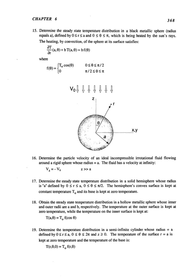
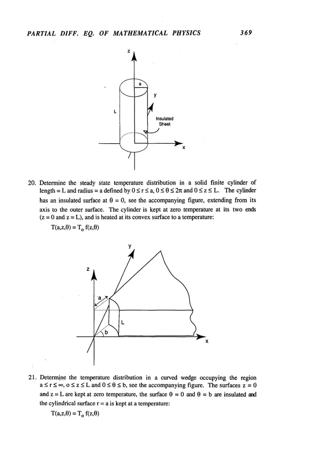
![CHAPTER 6
3 70
a a X
22. Determine
the temperaturedistribution in a hemi-cylinderof length = L and radius = a
defined by 0 < r < a, 0 < 0 < n and. 0 < z < L. Theconvexsurface at r = a, the two
plane surfaces at 0 = 0 and n and the lowerbase at z = 0 are kept at zero temperature,
whilethe upperbase at z = L is kept at a temperature:
T(r, 0,L)= Ofir,0)
Section 6.10
23. A metallic sphere of radius a and defined by 0 < r < a and 0 < 0 < ~t is kept at zero
temperature at its surface. A heat source is located in a spherical region inside the
sphere, suchthat:
V2T =-q(r, cos0) 0_<r<b
Find the steadystate temperaturedistribution.
24. Aspherical container is filled with a liquid whosewalls are impenetrable. If a point
sink of magnitude
Qexists at its center so that the velocity potential satisfies:
V2~= Qo ~(r) 0 _<r <a
4~r
2
Findthe velocity field inside the sphere.
25. A finite circular cylindrical container with impenetrable wails is filled with an
incompressibleliquid, occupyingthe space 0 < r < a and 0 < z < L. Apoint source and
a point sink of magnitudesQoare located on the axis of the cylinder at z = L/4 and
3L/4,respectively, suchthat the velocity potential ~(r,z) satisfies:
V2~I/= Qo~5(r)[~5(z-L/4)~5(z23L/4)]
"
2r~r
Findthe velocity field inside the container..](https://image.slidesharecdn.com/advancedmathematicalmethodsinscienceandengineering-hayek-230318001731-2b30ece5/85/advanced-mathematical-methods-in-science-and-engineering-hayek-pdf-383-638.jpg)
![7
INTEGRAL TRANSFORMS
7.1 Fourier Integral Theorem
If f(x) is a bounded
function in -~, <x < ~,, andhas at mostonly a finite number
ordinarydiscontinuities, andif the integral:
~lf(x)ldx
is absolutelyconvergent,then at everypoint x ~where
there exists a left andright-hand
derivative, f(x) canbe representedbythe followingintegral:
½tf(x+o)÷f(x-o)
- f( )cos(u(
O--e,~
Thefunction fix), -L _<x _<L, canbe representedbya Fourierseries as follows:
~[
f(x +O)+ f(x - 0)] =
where:
L
1
~f(~)
d~
-L
L
1 f(~)cos(~)d~
-L
~[a n cos(~ x)+ n sin(~x)]
n=l
L
1 ’f(~)sin(~)d~
bn -- -~
-L
Thus,addingthe twointegrals for an and bn gives:
L L
1 1
½[f(x+O)+ f(x-O,]:~- ~f(~)d~+ ~ r f f(~,cos(-~(~-x,)d~
-L n=l -L
383](https://image.slidesharecdn.com/advancedmathematicalmethodsinscienceandengineering-hayek-230318001731-2b30ece5/85/advanced-mathematical-methods-in-science-and-engineering-hayek-pdf-396-638.jpg)
![CHAPTER 7 384
n~ ~
un L and Aun = Un+l -- Un L
then the integrals canbe rewritten as:
+L +L
1
1~
f(x):-~ f f(~)d~+ 7 Aun ~ f(~)cos(un(~-x))d
~
-L n = 1 -L
Def’me
the integral to equalF(un), i.e.:
+L
= ~ f(~) cos(un(~ - x))
F(un)
-L
then the series convergesto an integral in the limit L --> ~ and Au
n --> 0 as follows:
~ F(un)Au n --> F(u)du
Lim
Au,-~0
n=l 0
Since the funcdonis absolutely integrablc, then the first termvanishes because:
+L
Lira ~ j f(x) dx ---> 0 and F(u) converges
L---~ 2L
-L
Thus,the representation of the function fix) by a doubleintegral becomes:
~[f(x+0,+ f(x-0)]= ~ ~ ~ f(~)cos (u(~-x))d~du
0-oo
cos(ux)du
+ sin u
n sin(ux)du (7.1)
7.2 Fourier Cosine Transform
If f(x) =f(-x) for -~,, <x <,,~ or, if f(x) =0 for the range_oo<x <0 where
one
choosef(x) = f(-x) for the range -~o< x <0, then the secondintegral in (7.1) vanishes
the integral representationcanbe rewritten as:
[f(x + O)+ f(x- 0)] f(~) cos(un~)d~ cos(ux)du x ->
OLO J](https://image.slidesharecdn.com/advancedmathematicalmethodsinscienceandengineering-hayek-230318001731-2b30ece5/85/advanced-mathematical-methods-in-science-and-engineering-hayek-pdf-397-638.jpg)
![INTEGRAL TRANSFORMS 385
Define the Fourier cosine transform as:
= I f(~)cos(u~)d~
Fo(u)
0
then, the inverse Fourier cosine transforms becomes:
f(x) = 2 ~ Fc(u) cos(ux)du
0
whereFc(u
) is an evenfunction of u and cos (ux) is known
as the kernel of the Fourier
cosine transform.
(7.2)
7.3 Fourier Sine Transform
If f(x) =-if-x) in -~, < x < ¢¢or if f(x) = 0 in the range-00 < x < 0, whereone
choosef(x) -- -f(-x) in the range-~ < x < 0, then the first integral of eq. (7.1) vanishes
~[f(x+
0)+ f(x- 0)] f(~)sin(u~)d~ x_>0
sin(ux)
Define the Fourier sine transform as:
= I f(~)sin(ug)d~
Fs(u)
0
then the inverse Fourier sine transform becomes:
0
whereFs(u
) is an oddfunction of u and sin (ux) is the kernel of the Fourier sine
transform.
(7.3)
7.4 Complex Fourier Transform
Theintegral representation in eq. (7.1) can be usedto developa newtransform.
Definethe function G
1 as the inner integral of eq. (7.1):
+~
l (U)I f(~) CO
S(U (~
- x))
G
then the function Gl(u
) is an evenfunction in u.](https://image.slidesharecdn.com/advancedmathematicalmethodsinscienceandengineering-hayek-230318001731-2b30ece5/85/advanced-mathematical-methods-in-science-and-engineering-hayek-pdf-398-638.jpg)
![INTEGRAL TRANSFORMS 389
Define the Hankeltransform F(p) as:
F(p) =~ r f(r) Jo(rP)dr
0
then the inverse Hankeltransform is given by:
f(r) = pF(P) Jo(rp)dp
0
(7.6a)
(7.6b)
7.7 Hankel Transform of Order v
Atreatment of Hankeltransformof order v similar to Hankeltransformof order zero
is givenin Sneddon.
Let f = f(x1, ~2..... Xn), then the Fourier transformandits inverse
weredefinedin Section7.5. If the functionf depends
on xl, x2 ..... xn as follows:
f : f(~/Xl~ +x2~+...+X~n)
then:
F(Ul,U
2 ..... Un)= f f ""ff(~x~+xi+’"+Xn2)el~XkUkdxldX2""dXn
Performinga similar coordinate transformation as wasdonefor the Hankeltransform,
define:
2
r 2 =Xl
2+x29+...+x
n
r2 = U~+u~ +... + U~n
with the following coordinate transformation:
Uk=
19a~k k =1, 2 ..... n
n
YJ = EaJ k xk J =1, 2 ..... n
k=l
In matrix notation, the transformationcanbe represented by:
[yj] =[ajkl[X
k]
such that the coefficients ajk, j ~ 1, are chosento make
the vector transformation
orthogonal,i.e., the matrix:
n n
{10 i=j
[ajk]=[ajk]-~ or Eajkaki = Eajkaik=~ji =
i~:j
k=l k=l](https://image.slidesharecdn.com/advancedmathematicalmethodsinscienceandengineering-hayek-230318001731-2b30ece5/85/advanced-mathematical-methods-in-science-and-engineering-hayek-pdf-402-638.jpg)
![CHAPTER 7 390
where~ij is the Kronecker
delta. Thus,the coordinatesxk are givenby:
Ixk] =[ajk]
~ [yj] =[akj]z [Yj]
r 2 =
n n n n n n n
E x2k = E E E [akjl[YJ ][ak/][y/l=E E [Yjl~J/[Y/]=E y~
k=l k=lj=l/=l j=l/=l /=1
The volume element becomes:
dx
1 dx2.., dx.={ [alj][dyj] } {[a2kl[dYk]
}... {[an/][dYl]
} =dy
1 dY2..,dy
n
Thus:
n n n n n n n
Eukxk= E E ukakJyJ :pE EalkakJyJ =pE ESlJYJ
=pyl
k=l k=lj=l k=lj=l k=lj=l
F(Ul,U
2 ..... Un)= f f ""ff(~12+z2)eipY~dYldy2""dYn
where:
z2 = y~ +y~2+...+y2
n
Onemustfind a function R, such that:
dy
2 dy
3 ... dy
n =Rdz
whereRis the surface area of a spherein n dimensionalspace:
F(Ul,U
2 ..... Un)= f ~-..j’f(~12+z2)eipYtRdzdyl
Toevaluate the formof R, start with the followingintegral:
J" J’... I F(4Y~+ Y~+.-.Y~n)dY2dY3""dyn
= ~F(z)Rdz
Since the volume
elementdy
2 dy
3 ... dy
n represents (n-I) dimensionalspace, let:
R= S z
n-2
Choose
F(z) = exp [-z2 ], then:
f ~ "’" ~ exp[-(Y22+ Y~+ ""y2n)] dY2dy3
"’’dyn = ~(n-1)/2
wherethe followingintegral wasused:
f exp[-x2,]dx =](https://image.slidesharecdn.com/advancedmathematicalmethodsinscienceandengineering-hayek-230318001731-2b30ece5/85/advanced-mathematical-methods-in-science-and-engineering-hayek-pdf-403-638.jpg)
![INTEGRAL TRANSFORMS 391
Theintegral for dz can be evaluated:
OO
I
S 1"(-~) n>2
exp[-z2 ] Szn-2dx= -~
0
Thus,the surface of a unit spherein n-dimensional
spaceis:
2 7t
(n-l)/2
S=
r’(-~)
so that the surface elementis givenby:
2~(n-l)/2 zn_2d
z
dY2 dY3"’" dYn = F(’-1)
Hence:
2~(n-1)/2 ~ If(~12+z2)ei0Yl zn-2dzdyl
F(Ul’U2..... Un)= F(-~) -oo
Let z = r sin 0, Yl = r cos 0. Thendz dy
1 = r dr dO,and the aboveequationbecomes:
2~t(n-l)/e rn-lf(r) Iei WC°S° (s
in0)n-e dOdr = F(9
F(ul,u~..... Un) = F(~)
0
Theinner integral becomes,(see equation 3.101):
1 n-1
Ieirpc°s0 (sin 0)n-2 dO=
n-2
where v = --, and n _> 1. Thus:
2
Jv(ro)
(2~)n/2rn/ 2f(r) Jv (rp) dr,
F(p) - v
0
Theinversion can be workedout in a similar manner:
n_>l
(2r0
n
... J F(9) e k=~duldU2...dun
--OO --OO
whichcan be shownto be equal to:
f(r) = 1 Ipn/2F(P)Jv(rp)d
p
(2~)n/2 v
0
Thus, combining
eqs. (7.7) and (7.8), one obtains:
(7.7)
(7.8)](https://image.slidesharecdn.com/advancedmathematicalmethodsinscienceandengineering-hayek-230318001731-2b30ece5/85/advanced-mathematical-methods-in-science-and-engineering-hayek-pdf-404-638.jpg)
![CHAPTER 7 394
Definethe following one-sidedfunction:
ev’x f(x) x >
_1
g~(x) = ~-~ f(0
+)
x = 0
lo x<0
vl>a (7.13)
g2(x)= ~ F_(u, v2)e-iUxdu (7.18)
Multiplyingeq. (7.17) by exp[vlx] and eq. (7.18) by exp[v2x], one obtains:
1 " °
eV’xgl(x)= ~-~ ~ F+(U,Vl)e-l(u+~v’)Xdu= x > 0 (7.19)
eV2Xg2(x): ~ f F_(u, v2)e-i(u+iva)Xdu x < 0 (7.20)
Combining
eqs. (7.19) ~md
(7.20), one canreconstruct f(x) again as definexl in eqs.
and (7.15):
wheregl(x) is absolutely integrable on [0,oo], then the Fourier transformof gl(x)
becomes:
F+(u, Vl)= f gl(~)eiU~d~= ~ gl (~)eiU~d~= f f(~)ei(u+ivi)~d~ (7.14)
Definethe followingone-sided function:
I0 x >0
g2(x) = tiff(0+) x=0 v2 > b (7.15)
/
[e-v2xf(x) x <
whereg2(x)is absolutely integrable over [-oo,0], then the Fourier transformof g2(x)
becomes:
0 0
F_(u, v2)= ~g2({)eiU~d{= ~g2({)eiU~d{= ~f({)ei(u+iv~)~d~
TheFourier inverse transforms of F+ and F_become:
gl(x)= .~ F+(U, vl)e-iUXdu (7.17)](https://image.slidesharecdn.com/advancedmathematicalmethodsinscienceandengineering-hayek-230318001731-2b30ece5/85/advanced-mathematical-methods-in-science-and-engineering-hayek-pdf-407-638.jpg)
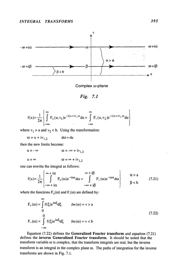
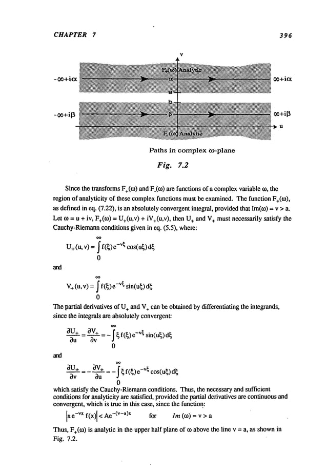
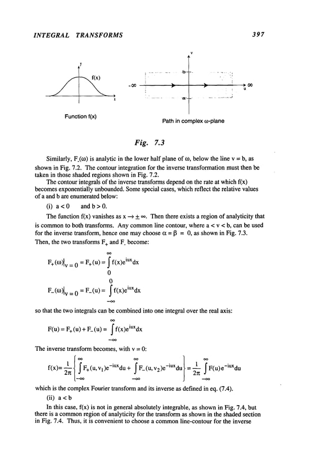
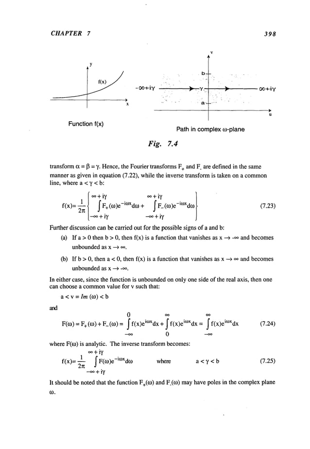
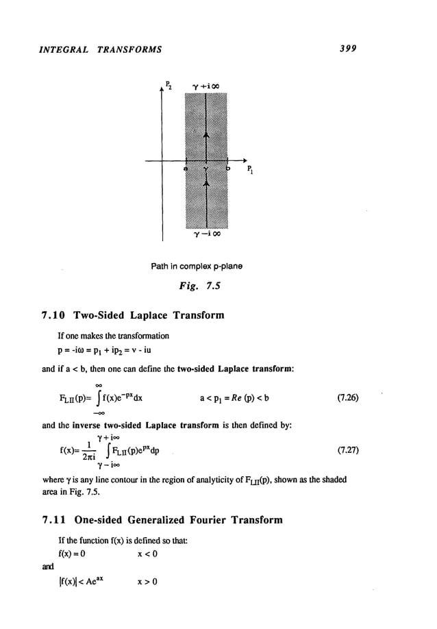
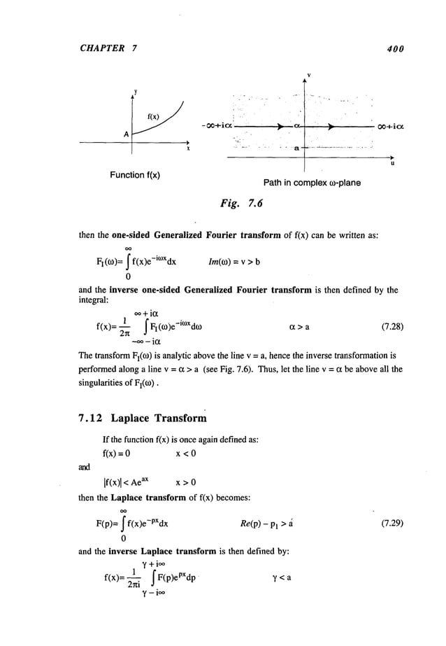
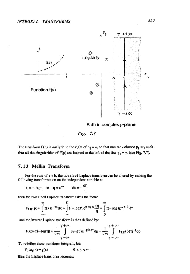
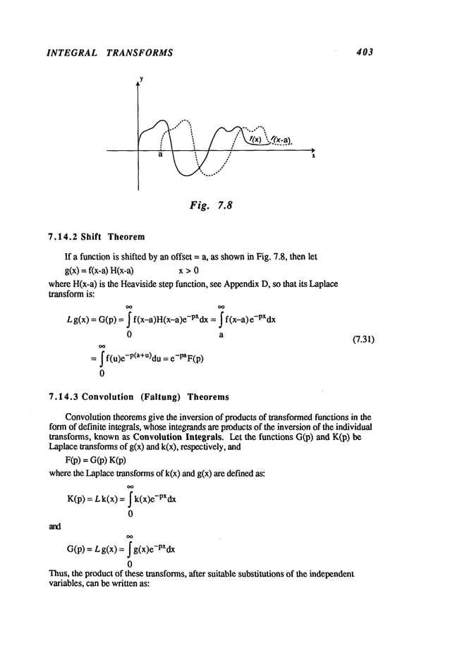
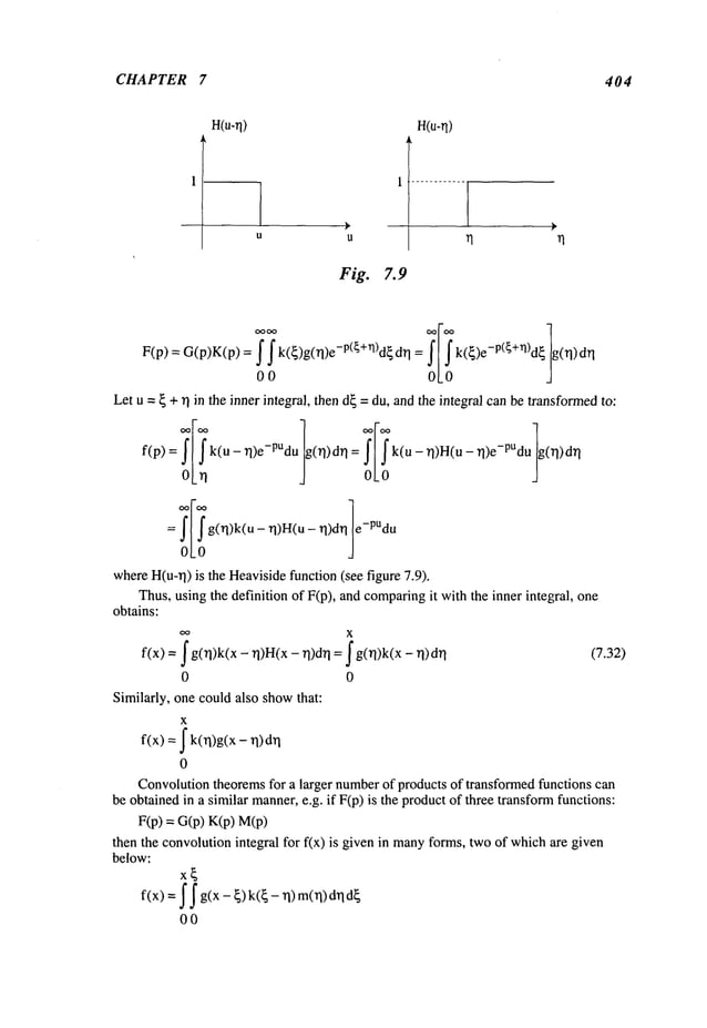
![CHAPTER 7 406
f(x)
t~(x) ~
[ f2(x) i f3(x) ! ’(x)
Fig. 7.10
x 2 x
L[x2 f(x)] = 2 f( x)e-px dX
=~dp f f( x)e-pX dxd2F
0 0
---’-
~
and, in general:
L[xn f(x)] = (-1)
n n_>0 (7.37)
dp
n
TheLaplacetransform of the Heavisidefunction H(x) is:
L [1] = L [H(x)] = 1/p
and that of a shifle.d Heaviside
function H(x-a)is:
e-Pa
L[H(x - a)] = e-PaL[H(x)] = (7.38)
P
whereequation (7.31) wasused. TheLaplacetransform of a powerof x is then derived
from(7.37) as:
n dd_~n (1)=
L[xn] = L[xnH(x)] = (-1)
~ pn+l
(7.39)
TheLaplac~transform of the Dirac Delta Function~(x) is (see Appendix
x
L[~i(x)] =_~5(x)e-px dx = e-PXlx= 0 = 1
0
Oneshouldnote that F(p) does not vanish as p -> ,~ becausethe function is a point-
function and does not conformto the requirementson f(x).
TheLaplacetransform of a shifted Dimc
function:
L [ 5(x - a)] = -pa (7.40)
7.14.7 Laplace Transform of Periodic Functions
Let f(x) be a periodic function, with a periodicity = T, as shown
in Figure 7.10i.e.:
f(x) = f(x+T)](https://image.slidesharecdn.com/advancedmathematicalmethodsinscienceandengineering-hayek-230318001731-2b30ece5/85/advanced-mathematical-methods-in-science-and-engineering-hayek-pdf-419-638.jpg)
 ~---~"/- D’(pj)~,P)/ j= 1,2,3 .... n
p--~pj[.
Theinverse transformF(p) can be readily obtained as the sumof the inverse of each
these terms:
n
f(x) = Z Aj pjx (7.42)
j=l
(ii) If only oneroot is repeatedk times, then, taking that root to be Pl, onecan
obtain the partial fractions as follows:
N(p)_ A~ A_
____2~2 At_
! A
k
F(P)=D(p) P-Pl (p-pl) 2 +"" ~ --÷Q(P)
(p-pl)
t-1 (p- pl)
k
whereQ(p)has poles at points other than Pl, i.e. simplepoles at Pt+l, Pt+2..... Pn" The
function Q(p)can be factored out as:
Q(p)- At+l Ak+2 ~. ..+ An
P- Pk+~ P- Pk+2 P-Pn
whichcan be treated in the samemanneras wasoutlined in section (i) above.
Letting G(p)= (p-pl)k F(p), then the constants 1 to A
t can be evaluated as
follows:
1 dG(Pl)
A
k : Lim[G(p)] = G(Pl) Ak_
1 =
p--~p~ 1! dp
1 d2G(Pl) 1 d(t-1)G(Pl
= AI=
Ak-2 2! dp 2 ..... (k-l)! (k-l)
1 d(k-J)G(Pl)
j = 1, 2 ..... k
Aj = (k-j)! (k-j)
To evaluate the contacts Ak÷
1 to A
n, one uses the sameformulaein (i). Thus, the
inverse transformof the part of the function F(p) corresponding
to the repeatedroot
takes the form:](https://image.slidesharecdn.com/advancedmathematicalmethodsinscienceandengineering-hayek-230318001731-2b30ece5/85/advanced-mathematical-methods-in-science-and-engineering-hayek-pdf-421-638.jpg)
![INTEGRAL TRANSFORMS 409
k
eP,X ,~a xj-1 d(k-J)G(Pt)
f(x) = j--’~l (j- 1)!(k- j)! (k-j) ~-q(x (7.43)
whereeqs. (7.39) and (7.36) wereused. Theremainderfunction q(x) is the sameas
in (7.42) with the index ranging fromj = k+l to
7.14.9 The Addition Theorem
If an infinite series of functionsfn(x) representinga functionfix):
O0
f(x)= Z fn(X)
n=0
is uniformly
convergent
on[0,,,o], andif either the integral of If(x)]:
Ie-PX dx
0
or the sumof the integrals of
Z I e-pxlfn (x)[dx
n=00
converges,then:
Lf(x)=F(p)=L Zfn(X)= ZLfn(X):
n=O n =0 n=O
"(7.44)
Example 7.1
Variousexamplesof the Laplacetransform, whichillustrate the various theorems
discussed above, are given below:
(i) sin (ax)H(x)’.
First, rewrite sin (ax) as a sumof exponentials:
1 , iax e-iax),
sin(ax)=~lte
then, using equation (7.36):
L[eiaXH(x)] _ 1
p-ia
TheLaplacetransformof sin(ax) is foundto be:
L[sin(ax)H(x)] = ~- pSia p+ia p2 2
(ii) bxsin(ax)
Since the Laplacetransform of sin(ax) is nowknown,one can use eq. (7.36) to evaluate
the product,i.e.:](https://image.slidesharecdn.com/advancedmathematicalmethodsinscienceandengineering-hayek-230318001731-2b30ece5/85/advanced-mathematical-methods-in-science-and-engineering-hayek-pdf-422-638.jpg)
![CHAPTER 7 410
L[ebxsin(ax)]= F(p- b) a
(p- b)2 + a
2
(iii) sin (ax)H(x)(periodicfunction):
Sincethe functionsin (ax)is periodicwithperiodicityT=2r4a, then:
2~/a
Fl(P)= fsin(ax)e-PXdx = p-~+a2(1-e-2pz/a)
0
then:
F(p) = Lsin(ax) - FI(P) a ~1 _-2pn/a, 1 a
- 1- e
-pT p - ) =p2+a’~-"T
a
(iv) Findthe inversetransformof F(p)= pXx :
F(p)canbewrittenas the productof twofunctions:
a a 1
F(p)=p2_a 2 p+a p-a
thenthe inversetransformof the productcanbeobtainedbythe convolution
theorem.
Letting:
a 1
G(p) = and K(p) =
p+a p-a
thenthe inversetransform
of G(p)andK(p)are known
to be(see eq. 7.53):
g(x) = -ax and k(x) = ax
so that the inversetransform
of F(p)canbeobtainedin the formof a convolution
integral:
X
f(x) = (a-an)(ea(x-rl))d~l =--~te-2ax- II = sinh(ax)
0
Alternatively,since the functionF(p) hastwosimplepoles whose
denominator
has
tworoots, p = + a, thenonecanusethe Heaviside
theorem
to obtainaninverse
F(p)= AI~ A2
p-a p+a
Sincetherootsaredistinctthen:
AI = 2~p 1
p=a 2
sothat:
F(p)= ’p
and
p=-a 2](https://image.slidesharecdn.com/advancedmathematicalmethodsinscienceandengineering-hayek-230318001731-2b30ece5/85/advanced-mathematical-methods-in-science-and-engineering-hayek-pdf-423-638.jpg)
![INTEGRAL TRANSFORMS 411
~[e ax - e-ax ] = sinh (ax)
f(x)
(v) Find the inverse transformof F(p), defined
p+a b;~c
F(p) = (P + b)(p 2
Thefunction F(p) has a simplepole at p = -b anda pole of order 2 at p = -c.
Let:
F(p)= A1 ÷ A2 + A3
p+c (p+c) 2 (p+b)
then the coefficients Aj are foundfromthe partial fraction theorem:
G(p)= (p + 2 F(p) = p + a ¯
p+b
Al=_~_p(_C)= b-a
_ b-a
a-c
A
2 = G(Pl) = G(-c) =
b-c
a-b
A
3 = (p + b) F(P)lp = (c- b)2
Thus,the inverse transformof F(p) is given by:
f(x) = ~__C{e-CXI-~-_
ca + (a - c) xl +e-bx~c_
whereeqs. (7.42) and (7.43) wereused.
7.15 ~ Solution of Ordinary and Partial Differential Equations
by Laplace Transforms
Onemayuse Laplacetransformto solve ordinary andpartial differential equationsfor
semi-infinite independentvariables. For use of Laplacetransform on time, wheret > 0,
onewouldrequire initial conditionsat t =0. In this case, application of Laplaceontime
for the first or secondderivations in timerequires the specification of oneor twoinitial
conditions, respectively, as required by the uniquenesstheorem.Useof Laplacetransform
on space is moreproblematic. Useof Laplaceon x for the secondderivative ~2y(x,t)/~x2
wouldrequire the specification of y(0,t) and by(0,t)/~x. However,
uniquenesstheorem
requires that only one of these twoboundary
conditionscan be specified at the origin.
Hence, one must assumethat the unknown
boundarycondition is a given function. For
example,if y(0,t) = f(t), a specified function, then onemustassumethat 3y(0,t)/3x =
an unknown
function. Thefunction g(t) must be solved for eventually after finding
y(x,t) in termsof g(t). Thereverse would
also be true: if 3y(0,t)/0x = f(t),
y(0,t) = g(t); an unknown
function. This indicates that the Laplacetransformis
suited to use ontime rather than space.
In this section, the Laplacetransformwill be applied onvarious ordinaryor partial
differential equations in the followingexamples.](https://image.slidesharecdn.com/advancedmathematicalmethodsinscienceandengineering-hayek-230318001731-2b30ece5/85/advanced-mathematical-methods-in-science-and-engineering-hayek-pdf-424-638.jpg)
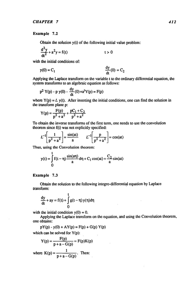
![INTEGRAL TRANSFORMS 413
t
y(t) =J f(t - q) k(rl)
0
Example 7.4
Obtainthe solution to the followinginitial value problemby use of Laplacetransform:
d2Y ~tdY_2y=l
dt 2 dt
withthe initial conditionsof:
t>0
y(O)=O dY(o)
dt
Applyingthe Laplacetransform to the equation, and noting that the equation has non-
constant coefficients, the Laplacetransformfor It y’(t)] becomes:
L[t-~tI=-d[LdYl=--~p[PY(P)-Y(O)]=-PdY-YdpI_
dt J dp
then:
dY
p2y_ py(0)- -~tY(0) - p-~-p - Y- 2Ylp
or:
The homogeneoussolution Yh becomes:
Yh
=
and the particular solution Yparis foundto be:
1
Ypar = ~
Thus,the total solution can be written as follows:
e p2/2 1
Y= ~+ p3
C p3 --
Since the limit of Y(p)goesto zero as p goesto infinity, then C= 0 and Y(p)= 3.
Theinverse transformgives (see eq. 7.39):
t
2
y(t) =
2
Example 7.5 ForcedVibration of a Stretched Semi-infinite String
Asemi-infinite free stretchedstring, initially undisturbed,is beingexcitedat its end
x =0, suchthat, for y = y(x,t):](https://image.slidesharecdn.com/advancedmathematicalmethodsinscienceandengineering-hayek-230318001731-2b30ece5/85/advanced-mathematical-methods-in-science-and-engineering-hayek-pdf-426-638.jpg)
![CHAPTER 7 414
O2y_ 1 ~)2y
x>0 t>0
~)X2 - C2 Ot
2
together withthe initial and boundary
conditions:
y(O,t)=f(t) y(x,O
÷) =0 ~ (x,O÷) = 0
Ot
Thedifferential equationsatisfied by the string is first transformed
onthe time
variable,that is:
wherethe symbolL
t signifies Laplacetransformationon the variable t. Let:
OO
Y(x,p) = I y(x, t) e-Ptdt
0
then the transformof the partial derivatives onthe spatial variable x is:
and the transformof the partial derivative onthe time variable is:
I~)2Yl ~Y (x,0+)] p2y
P2y-[py(x’0+)+Ot
=
Transformingthe boundarycondition at x = 0:
L
t y(0, t) =Y(0,p) = L
t f(t) = F(p)
Thus, the systemtransforms to the following boundaryvalue problem:
d2y p2 Y = 0
dx 2 c
2
Y(0,p) = F(p)
Thesolution of the differential equationcan be shown
to be:
Y = Ae-P
x/c + Be
px/c
Thesolution Ymust vanish as x ~ oo, whichrequire that B = 0. Theboundarycondition
at x = 0 is satisfied next:
Y(0,p) = A = F(p)
so that the solution in the transformplane is finally foundto be:
Y = F(p)e-P
x/c
Theinverse transformis given by:
If(t
- x) t >x/ c
y(x, t) = 1 [F(p)e-px/c] =l0 c
t < x/c
whichcan be written in terms of the Heavisidefunction:](https://image.slidesharecdn.com/advancedmathematicalmethodsinscienceandengineering-hayek-230318001731-2b30ece5/85/advanced-mathematical-methods-in-science-and-engineering-hayek-pdf-427-638.jpg)
![INTEGRAL TRANSFORMS 415
y(x, t) = f(t - x) H(t
C C
wherethe shift theorem(eq. 7.31) wasused. Thesolution exhibits the physical property
that any disturbanceat x = 0 arrives at a station x at a timet = x/c havingthe sametime
dependence
as the original disturbance.
Example 7.6 Heat Flowin a Semi-infinite Rod
Obtainthe heat flowin a semi-infinite rod, whereits endis heated, suchthat:
T= T(x,t)
~2T 1 3T
x>0 t>0
~x 2 K ~t
subject to the followinginitial andboundaryconditions:
T(0,t)fit) T(x,0
÷)=0
Applyingthe Laplacetransform on t on the equation, and defining:
T(x,p) = fT(x,t)e-Ptdt
0
then the equation and the boundarycondition transformto:
d2Y ~[pY-T(x,O)]
r=
K
Y(O,p) = FCp)
Thedifferential equation on the transform temperatureT becomes:
" ET=
0
dx 2 K
and has the twosolutions:
y = Ae- p~-~x + Be+.~-~/Kx
Boundedness
of T as x ---> ,~, requires that B= 0. Satisfying the boundary
condition:
Y(O,p) = F(p)
then, the solution in the complex
plane p is given by:
Y = F(p)e- P~~X
Theinverse transform of exp [-~/~/K x] [from Laplace TransformTables] is given as
follows:
L-l[e-a~/~ 1= ~ea -a2/4t where a = ~
Thus, using the convolutiontheorem(eq. 7.32):](https://image.slidesharecdn.com/advancedmathematicalmethodsinscienceandengineering-hayek-230318001731-2b30ece5/85/advanced-mathematical-methods-in-science-and-engineering-hayek-pdf-428-638.jpg)
![CHAPTER 7 416
=~- f(t- 4K{~)e ~ d{- - 4-~-~)e -~ d~
If f(0 =To= constant, then the integral canbe solved:
T(x,t)=-~-~ e-~d{- e-{~d{ =T~[1- Toerfc(x)
0
whereeft(y) is the error function as definedin B5.1(Appendix
B) anderfc(y) = 1 -
anderf (0,,) =
Example 7.7 Vibration of a Finite Bar
Afinite bar, initially at rest, is induced
to vibrationbya forcef(t) appliedat its end
x -- L for t > 0. Thebar’s displacementy(x,t) satisfies the followingsystem:
32y 1
3x~ = ~ 3t
2
y(O,0
= y(x,0
÷)=o
~t (x,0+) = AE-~xY
(L,t) =f(t)
ApplyingLaplacetransform on the time variable, the equation transforms to:
~d2Y = ~2[p2Y(x,
p) - py(x,0+
)- O.~Y
(x,0+)]
=P-~2
,,,, (x,p) ot c
~
whereY(x, p) = Lt y(x,t). Transformingthe boundaryconditions:
_~_ F(p)
Y (0,p) = 0 and (L, p) =
Thesolution of the differential equation on the transformedvariable Ycanbe written as
follows:
Y(x,p) = -px/e + Be
+px/¢
whichis substituted in the twoboundaryconditions:
Y (0,p) = D + B=](https://image.slidesharecdn.com/advancedmathematicalmethodsinscienceandengineering-hayek-230318001731-2b30ece5/85/advanced-mathematical-methods-in-science-and-engineering-hayek-pdf-429-638.jpg)
![INTEGRAL TRANSFORMS 417
~
_x (L, p) P [_De-PL !
c +Be
+PL !c ] _ F(p)
c AE
Theunknown
coefficients are readily evaluated:
c F(p)
B=-D=
p AE e-pL/c +e
+pL/c
and the transformedsolution has the form:
c F(p) e+px/c -e
-px/c
V(x, p)
p AE e+PL/C+e
-p L/c
Separatingthe solution into twoparts:
Y(x, p) = ~EEF(p) G(x,
whereG(p)is definedas:
1 e+pX/c- e
-px/c Gl(X,p)
G(x,p) =
p e+pL/c + e-pL/c 1 - e
-4pL
/c
whereGl(X,p)represents the transformof the first part of a periodic function whose
periodicity is T = 4L/cand is givenby:
G
l(x, p) = 1 [e_P(L_x)/c_ e_P(x+L)/c_ e_P(aL_x)/c+ e_P(aL+x)/c
P
Theinverse transformof eap/pis H(t - a) whichresults in an inverse of Gl(X,
gl(x, t) =H[t (L
- x) / c] - H
[t- (L÷ x)
-H[t- (3L- x) / c] + H[t - (3L+ x)
Theinverse transformof G(x,p) is given by g(x, t) where:
g(x,t) = gl(x,t) 0 _<t <4L/c
andg(x, t) is a periodicfunction withperiodT =4L/c, i.e.:
g(x,t) = g(x,t+4L/c)
so that the periodicfunction canbe written as:
g(x,t)= E gt(x’t-4nL/c)
n=0
Thefinal solution to the displacementy(x, t) requires the use of the convolutionintegral:
t
c
I
y(x, t) = -~ g(x, u)f(t-
0
If fit) = o =constant, then F(p) = Fo
/p, an
c Fo e+px/c -e
-px/c
Y(x,p)= p2 AE+pL/c +e
-pLlc
Thetransform of the deformationat the end x = L then becomes:](https://image.slidesharecdn.com/advancedmathematicalmethodsinscienceandengineering-hayek-230318001731-2b30ece5/85/advanced-mathematical-methods-in-science-and-engineering-hayek-pdf-430-638.jpg)
![CHAPTER 7 418
h(x)
T/2 T 3T]2 2T 5T/2
Fig. 7.11
Thetransformof a SaWmtOOth
(triangular) waveh(x) definedby ), 0 _<
x <_T,(as
shown
in figure 7.11) is definedas:
=~2x/T
0<x<T/2
hi(x)
2(1-x/T) T/2_<x<T
L h(x)= 2,,tanh(PT)
Tp~ 4
Thus, the inverse transform of the deformationbecomes,with T = 4L/c:
y(L, t) = 2 h(t) = dynamic
deflection/static deflection
Yo
whereYois the static deflection definedby:
Themaximum
value y(L, t) attains is o att =2L
/c, 6L/c..... Thedeflection at any
other point x can be developed
in an infinite series form:
c Fo e-p(L-x)/c -e
-p(L+x)/c
Y(x,p)= p2
I+e-2P
L/c
Y(x,p) c U’x " c Ul(x,p)
=~ [ ’P)=~I -4pL/e
Yo -
U
1 (x,p) = -~1 Ie-P(L-x)/c -p(x+L)/c - e -p(3L-x)/e + e-p(x+3L)/e
]
p2 L
whereU(x,p) represent a periodic function, u(x,t) = u(x,t + 4L/c) 1 being the
transformof the function u(x,t) withinthe first period 0 _<< 4L
/c. Noting that fr om
equation 7.3 h
L-1[~-~Ze-aP]=(t - a) Hit-
then, the solution y(x,t) is givenby the periodicfunction u(x,t) = u(x, t + 4L/c):](https://image.slidesharecdn.com/advancedmathematicalmethodsinscienceandengineering-hayek-230318001731-2b30ece5/85/advanced-mathematical-methods-in-science-and-engineering-hayek-pdf-431-638.jpg)
![INTEGRAL TRANSFORMS 419
Yn/Y0
Y/Y0
/ (L+x)/c (3L-x)/c ~
I I~ I I,, I r ~,
2x/L
(L-x)/c L/c (L+x)/c 2L/c (3L-x)/c 3L/c (3L+x)/c
T= period = 4L/c )
Fig. 7.12
y(x,p) c
~o =~u(x,p)
Theinverse transformof Ul(X,p) is then foundas:
ul (x, t) = [(t- L - X)H(t- L - x) _ (t - L + X)H(t
C C C C
-(t- 3L- X)H(t_3L- x)+ (t- 3L + X)H(t_3L +..__.~x)]
C C C C
for 0 _<t < 4L/c.
Thesolution ul(x,t) for the first period< t < 4L
/c is mad
e up of thefirs t arri val of
the waveat t = (L - x)/c whichis then followedby three reflections, twoat x = 0 andone
at x = L. This solution is shown
graphically for the first periodt = 4L/c in the
accompanying
plot, see Fig. 7.12. Notethat from that time on, the displacementis
periodic with a periodof T = 4L/c.
Useof the Laplacetransformonthe time variable t requires that twoinitial values be
given, whichare required for uniqueness. However,
use of the Laplacetransform on the
spatial variable x, requires twoboundaryconditionsat x = 0, of whichonly one is](https://image.slidesharecdn.com/advancedmathematicalmethodsinscienceandengineering-hayek-230318001731-2b30ece5/85/advanced-mathematical-methods-in-science-and-engineering-hayek-pdf-432-638.jpg)
![CHAPTER 7 420
prescribed. Onecan solve such problems by assumingthe unknown
boundarycondition
and then solve for it, by satisfying the remainingboundarycondition.
Example 7.8 WavePropagationin a Semi-Infinite String,
Asemi-inf’mitesuing, initially at rest, is excited to motion
by a distributed load
applied at t = to and givena displacementat x = 0 such that the displacementy(x,t)
satisfies:
32__ff_y
=._~_1~
~2~y
+poe_bX
8(t-to)
~x 2 c" 3t ~ To
y(0,t) =YoH(t)
x > 0 t,t o >0
y(x,O
÷) =0 ~ (x,O÷) =0
ot
Obtainthe solution y(x, t) by using Laplacetransformonthe spatial variable
Define the Laplacetransform on x:
L
x [y(x, t)] = Y(p, t)= ~y(x, t)e-PXdx
0
Applyingthe Laplacetransformon the differential equation:
3y(0,t) 1 d2Y(x,p) Po ~i(t-to)
p2y(x,p)- py(0,t) +
bx =~’~ dt
2 To p+b
Since the displacementat x = 0 wasgiven, but not the slope, 3y/~x is not known,then
assumethat:
~(O,t) = f(O
so that the differential equationtakes the form:
d2y _
d7 c2p2y = -c2p2y° H(t)- c2f(t)- 2 Po ~(t- t o) = Q(
To p+b
The homogeneous
and particular solutions arc given by:
Yh= A sinh (cp0 + Bcosh (cpt)
t
Yp= 1 f Q(u) sintcp(t - u)]du
cp~)
= Yo(1 - cosh(cpt)) - ~ ~ sinh[cp(t- u)] H[t
P ¯ PtP+ o) ~o
t
_c [ f(u)sinh[cp(t-
u)]du
Usinginitial conditions:
Y(p,0) = 0 =](https://image.slidesharecdn.com/advancedmathematicalmethodsinscienceandengineering-hayek-230318001731-2b30ece5/85/advanced-mathematical-methods-in-science-and-engineering-hayek-pdf-433-638.jpg)
![INTEGRAL TRANSFORMS 421
dY(p, O) =pcA=
dt
so that Y(p,t) = Yp(p,t). Theinvers~transformof Y(p,t) is then given
t
0
CPoH[t - toil1- e-blx+c(t-t°)l]H[x + c(t-to)]
2bTo
+ cP° Hit - to][l- e-b[x-c(t-to)l]H[x - c(t-to)]
2bTo
Thesolution for y(x.t) still contains the unknown
boundarycondition f(0.
Differentiating y partially withx and setting x =0 one obtains:
t
~B~x-Yx
<0.t, =f(t)=--Y2-°-8(ct, - ~ J f(uXS[c(t-u)]
- 8[c<u-t,])du
0
CPo Hit-to](bc
-be(t-t°)
+2sinh[bc(t-
to)gi[c(t-to)]/
2bTo !
where~(u) = ~(-u) and ~(cu) = 5(u)/c wereused (Appendix
Theintegral in the last expressioncanlx~ shown
to equalf(t)/2, so that f(t) is finally
obtainedas:
f(t)= - ~ 8(t) cP°H[
t - to1(b-be (Ho)
+ 2 sinh [bc(to)]8[c(t -to)])
z bl
0
Substituting f(t) into the integral t~rmof y(x, t) results in the followingexpression:
Y._~o
H[ct- x] - _c.P_
° H[c(t- o) -x]H[t - to] (-b[x-~(t -to)] _ l)
2 2blo
Substituting the last expressioninto that for y(x, t) gives a final solution:
y(x,t) = yoH[ct- x]- cP° H[t- to]e-bx sinh[bc(t- to)]
bTo
+ ¢Posinh[b~(t- to) - b×] H[(t- to)- x
bTo
whereH(-u) = 1 - H(u)wasused in the expression.
7.16 Operational Calculus with Fourier Cosine Transform
TheFourier cosine transformof a function f(x) wasdefined in 7.2 as follows:
oo
Fc[f(x)] = Fc(u)= ]f(x)cos(ux)dx
0
then:](https://image.slidesharecdn.com/advancedmathematicalmethodsinscienceandengineering-hayek-230318001731-2b30ece5/85/advanced-mathematical-methods-in-science-and-engineering-hayek-pdf-434-638.jpg)
![CHAPTER 7 422
7.16.1 Fourier Cosine Transform of Derivatives
TheFourier transformof the derivative of f(x) is derivedas:
u
I
= = f(x)cos(ux)l 0 + f(x)sin(ux)dx
J Ox
0 0
= uFs(u
) - f(0
+)
Thetransformof the secondderivative of f(x):
°~ ~2f~(2x) ~.x cos (ux) ~ Of
~3~
32f(x)
cos (ux) + u sin (ux)
Fc[0--~-l=J 3x =
0 0
=-~O-~-f
(0+)+u
f(x)sin
(ux)l~
2f f(x)cos (u
x)dx
OX ~
0
= -U2Fc(u) - ~ +)
In general, the Fourier cosinetransfo~ of evenandoddderivatives are:
02nf
n - 1
02n_2m_lf(0+)
Fc[~] = (-1)nu2nFc(U)- ~ (-1)mu 2m 0x2n_2m_
1
n ~ 1
m=0
and
3mf
providedthat 3x
m--) 0 as x --) ,~ for < (2n-l)
~)2n+lf n
~)2n_2mf(0+
)
Fc[ff I = (-1)nu2n+lFs(u)- (- 1)mu2m" 3x2n-2m
m=0
n_-’:.0
(7.45)
providedthat 3x
m~ 0 as x ---) oo for m_<2n (7.46)
It shouldbe notedthe Fourier cosinetransformof evenderivatives of a function gives
the Fouriercosinetransformof the function, andrequires initial conditions.of odd
derivatives. However,
the Fourier cosine transformof oddderivatives leads to the Fourier
sine transformof the function, and henceis not conduciveto solving problems.](https://image.slidesharecdn.com/advancedmathematicalmethodsinscienceandengineering-hayek-230318001731-2b30ece5/85/advanced-mathematical-methods-in-science-and-engineering-hayek-pdf-435-638.jpg)
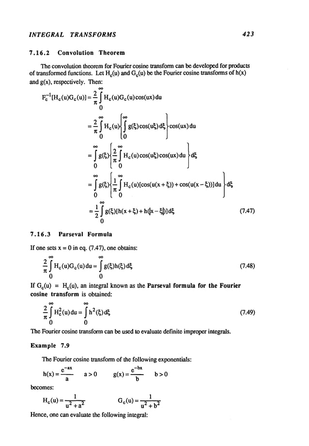
![CHAPTER 7 424
du rc e-ax e
-bx
0 (u2 + a2)(u2+a2) " a b
0
byuseof eq. (7.48).
dx =
2ab(a+ b)
Example 7.10 HeatFlowin Semi-Infinite Rod
Obtain
the heatflowin a semi-infinite
rod, initially at zerotemperature,
where
the
heatfluxat its endx =0 is prescribed,
suchthat thetemperature
T=T(x,t)satisfies the
followingsystem:
~2T 1 ~T
x>0 t>0
3-"~" = K3t
-~xT
(0,t)
= T(x,0+) = limT(x,t)-->
/(t)
Sincethe Fouriercosinetransform
requiresodd-derivative
boundary
conditions,see
Equation
7.45, it is wellsuited for applicationto the presentproblem.
Defining
the
transform
of the temperature:
T(u,t) = ~T(x,t) cos(ux)
0
thentheapplicationof Fouriercosinetransform
to the differentialequation
andinitial
condition
resultsin:
EI~2T]=-u2r-~xT(0,t)=-u2~+/(t) F[OT~= 1dr
Lax
J °LaxJ
F¢[T(x,0+)]= T(u,0+) = 0
Thus,the equationgoverning
the transform
of the temperature:
dT
K/(t)
l- u2Ky
=
dt k
canbewrittenas anintegral,eq. (1.9):
t
= Ce
-u2Kt
+ --~-J/(t- TI)e
-ku211
dT
I
T(u,t)
0
which
mustsatisfy theinitial condition:
T(u,0+) = C = 0
Thus,the solutionis found
in the formof anintegral:
t
T(u,t)= -~ ~/(t- rl)e
-kuhl
0
Applying
the inversetransformation
on the exponential
functionwithinthe integrand:](https://image.slidesharecdn.com/advancedmathematicalmethodsinscienceandengineering-hayek-230318001731-2b30ece5/85/advanced-mathematical-methods-in-science-and-engineering-hayek-pdf-437-638.jpg)
![INTEGRAL TRANSFORMS 425
Usingintegral or transformtables:
1 ~" _x
~/4a
I<x>
=e cos<ux
du--
i
0
onefinally obtains the solution:
~2! l(~)e-X2/(4K~l)
T(x,t) ~ d~
7.17 Operational Calculus with Fourier Sine Transform
TheFourier sine transform, as definedin 7.3, will be discussedin this section. Let
the Fourier sine transformof a functionf(x) be definedas:
Fs[f(x)] = Fs(u)= ~ f(x)sin(ux)dx
0
then:
f(Ixl)sgnx=~ Fs (u) sin(ux)
du
0
wherethe signumfunctions sgn is defined by:
sgn(x)= {;/Ixlx=0
x,O
7.17.1 Fourier Sine Transform of Derivatives
TheFourier sine transformof the derivative of f(x) canbe derivedas:
-- OxF~
[--~] =~0f(x)f ~ sin(ux)dXox
=f(x) sln(ux~0" oo_ u~f(x)cos(ux)dx
=-uFc
0 0
Thetransformof the secondderivative of f(x):
F[
o2f(x)ls
Ox
2j: ~O2f(~x)
sin(ux)dx
=Of
"’~
3x" ~xx
s,n(uxl
~- u*OOf~
~xx
cos(ux)dx
0
0 0
=0- uf(x)cos(ux)10
u f(x)sin (u
x)dx= -uZFs(u)
+ uf(0
+)
0](https://image.slidesharecdn.com/advancedmathematicalmethodsinscienceandengineering-hayek-230318001731-2b30ece5/85/advanced-mathematical-methods-in-science-and-engineering-hayek-pdf-438-638.jpg)
![CHAPTER 7 426
and ingeneral:
~2nf
Fs [~-~] = (-1) n u2nFs(u)
n
X (-1)m+lu2m-I o2n-2mf(0+)
~x2n-2m
m= 1
n_-’:
1
~mf ^
~ovided that ~ ---> t~ as x ~oo form < (2n-l)
~2n+lf n
FS[~x-~ "~] = (-1)n+l u2n+lFc(u) + X (-l)m+l °~2n-2 m+lf(0+)
~x2n-2m+l
m=l
(7.50)
n_>l
~mf
~ovided that ~ ~ 0 as x ~ oo for m _< 2n (7.51)
It shouldbe notedthat the Fourier sine transformof evenderivatives of a function
give the Fourier sine transformof the function, and requires initial conditionsof even
derivatives. TheFourier sine transformof oddderivatives give the Fourier cosine
transformof the function, and thus cannotbe used to solve problems.
7.17.2 Convolution Theorem
It can be shown
that there is no convolutiontheoremfor the Fourier sine transform.
Let H
s (u) and s (u) be t he Fourier s ine t ransforms o
f h(x) and g(x) r espectively. T
oo
F~-I [Hs(u)Gs(u)] =.-~ f Hs(u)Gs(u)sin(ux)du
0
= j" g(~ j" H~(u)sin(u~)sin(ux)du
0 ~ 0
whichcannot be put in a convolutionform, since the integrals are cosine and not sine
transforms.
If H
s (u) and c (u) are t he Fourier s ine t ransform o
f h(x) and the Fomier c
osine
transformof g(×), respectively, then the inverse sine transformof this productbecomes:](https://image.slidesharecdn.com/advancedmathematicalmethodsinscienceandengineering-hayek-230318001731-2b30ece5/85/advanced-mathematical-methods-in-science-and-engineering-hayek-pdf-439-638.jpg)
![INTEGRAL TRANSFORMS 427
Fs-l[Hs(U)~c (u)] : ~ f Hs(U)~¢(u)sin(ux)
0
c (u sln(u sln(ux)
= fh(~).
0
= f h(~)
-~Gc(U)sin(u~)sin(ux)du
0
I
f Gc(u)[cos(u(x - ~)) - cos(u(x + ~))]
0
= -~ h(~)[g([x - ~1) - g(x + (7.52)
0
Thismeansthat if there is a productof twofunctions, Fl(U).F2(u
), then call Fl(U)
Hs(u), and F2(u) = Gc(u). Touse the convolutiontheoremuse the inverse transform
h(x) = -1 (H
s(u)), an
d that ofg(x) = F-1(G
c (u)),to obtainh(x) an
d g(x
7.17.3 Parseval Formula
Considerthe followingintegral:
~ffHs(u)Gs(u)c°s(ux)du=--2n! Hs(u)0 g(~)sin(u~)d~ cos(ux)du
= f g(~) ~ Hs(u)sin(u~)cos(ux)du
0 [ 0
= bg(~) Hs(u)[sin(u(x+{))+sin(u(~-x))]du
0
= -~ g(~)[h(x + ~) h(lx- ~[)Sgn(~ - x)
0
If x is set to zeroin (7.53), oneobtains:
f Hsu)Os(u)au=
0 0
and if Hs(u)= Gs(u), then:
(7.53)
(7.54)](https://image.slidesharecdn.com/advancedmathematicalmethodsinscienceandengineering-hayek-230318001731-2b30ece5/85/advanced-mathematical-methods-in-science-and-engineering-hayek-pdf-440-638.jpg)
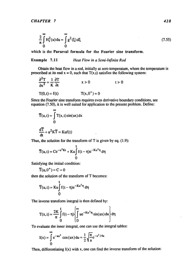
![1NTEGRAL TRANSFORMS 429
dx 4a ~/a
0
so that the solution of the temperatureis given by:
t
¯(x,t)--~~f(t-n)n-3~2e
-~2
~(4~:~)
0
Compare
this result with the result of Example
7.5.
Example 7.12 FreeVibration of a Stretched Semi4nfinite String
Obtainthe amplitudeof vibration in a stretched, flee, semi-infinite string, suchthat,
y =y(x,t) satisfies the followingsystem:
02y_ 1 O2y
~-~-r-
~-~-
t x>0 t>0
y(0,t) = lira y(x,t) -->
X---> ~
y(x,0
÷)=fix) ~-t (x’0÷)=g(x)
Since the boundarycondition is an evenderivative, then apply Fourier sine transformto
the system. DefiningY(u,t) as the transformof y(x,t), then application of Fourier
transformto the differential equationandthe initial conditionsresults in:
--7
L~x"
J
Fs[Y(X,0+)]= Y(u,0
+) = Fs(f(x)) =
Ldt J dt
Thus,the transformed
systemof differential equationand initial conditions:
d2Y 2 2,, dY
~+c u ~=0, Y(u,0
+)=F (u ~(u,0 +)=G(u)
Y= Asin (uct) + Bcos (uct)
Satisfying the twoinitial conditionsyields the final transformedsolution:
Y(u, t) =G(u)sin(uct) + F(u)
uc
and the solution y(x, t) can nowbe written in termsof twoinverse transformintegrals:
y(u,t) 2 ~ G(
u)sin(act) si n(ux) du
+ 2
_.~ F(u)cos(u
ct) sin(u
~ uc ~
0 0
Thesecondintegral can be evaluatedreadily:](https://image.slidesharecdn.com/advancedmathematicalmethodsinscienceandengineering-hayek-230318001731-2b30ece5/85/advanced-mathematical-methods-in-science-and-engineering-hayek-pdf-442-638.jpg)
![CHAPTER 7 430
~ ~F(u)cos(uct)sin(ux)1~~ F(u
)[sin(u(x + ct)
)+sin(u(x- ct))]
0 0
=~ [f(x+ ct) f(lx- ctD Sn
g(x - ct)]
Thefirst integralcanb~evaluated
as follows:
1
- I G(u)
[cos(u(x
- ct) - cos(u(x
+ ct))]
g- u
0
Since:
g~vDSgn
v = ~ 7 g(u) sin(uv)
0
then:
lg(~ql)Sgn’qdrl:~G(u ) sin(url)d~ i du=- G(U)c°s(uv)dUu
0 0 (0 J 0
whereF=--2 ~ G(u) du.
~ u
0
Thus:
oo v 0
_21 G(u)cos(uv)du: _j’g(lrll)Sgn+F= j"
g(]rll )drl + F
~ U
o o Ivl
Thefirst integral thenbecomes:
~-O-~ [cos(u(x- ct)- cos(u(x + ct))]du
0
+F
x+ct
1
=~’c J" g(rl)d’q
Thus,the total solutionbecomes:
x+ Ct
1
y(x,t)=~[f(x+ct)+f(~x-c~)Sng(x-ct)]+’~c ~](https://image.slidesharecdn.com/advancedmathematicalmethodsinscienceandengineering-hayek-230318001731-2b30ece5/85/advanced-mathematical-methods-in-science-and-engineering-hayek-pdf-443-638.jpg)
![INTEGRAL TRANSFORMS 431
7.18 Operational Calculus with Complex Fourier Transform
ThecomplexFourier transform wasdefined in eq. (7.4). Let F(u) represent
complex
Fourier transformof fix), defined as follows:
F(f(x)) = F(u) = ~ iux dx
then:
f(x) = -~ F(u)e -iux du
7.18.1 Complex Fourier Transform of Derivatives
Thecomplex
Fourier transformof the first derivative is easily calculated:
OO OO
~ ~ ~f iux f(x)eiuxl~** ~
F[ ]= ~xx e dx=
_ - f(x)e
iu xd x=(-iu)F(u)
Thetransformof the secondderivative of f(x) is:
F[ ~--~-] =~2f~32f~~x
2 eiUX
dx = ~x-fxeiUX-iu~~f iux
: -iu feiuxl_ L -iu!_ feiux dx = (iu)2F(u)
In general:
~nf = (-iu)nF(u)
n > 0
FtO- -
providedthat 13xm
I --> 0 as x --> ~ for m_<(n-l) (7.56)
7.18.2 Convolution Theorem
TheConvolutiontheoremfor the complexFourier transform for a product of
transforms is developedin this section. Let F(u) and G(u) represent the complex
Fourier
transformof f(x) and g(x), respectively. Then,the inverse transformof the product
definedas:](https://image.slidesharecdn.com/advancedmathematicalmethodsinscienceandengineering-hayek-230318001731-2b30ece5/85/advanced-mathematical-methods-in-science-and-engineering-hayek-pdf-444-638.jpg)
![CHAPTER 7 432
F-1 [F(u)G(u)] = ~ F(u)G(u) -iux du
= ~_~.~F(u iu~ - "
e lux du
= ~ g F(u)e -iu(x-~ d~
= ~ g(~)f(x- ~)
Similarly, it can be shown
that the last integral can also be written in the form:
~ f(~)g(x - ~)
7.18.3 Parseval Formula
(7.57)
If onesets x =0 in eq. (7.57) oneobtains:
__1 ~ F(u)G(u)du= g(~)f(-~)d~= g(-~)f(~)d~
(7.58)
2g
whichdoes not lead to a Parseval formula. However,
if one defines the complex
conjugateof G(u) as follows:
G*(u) = ~ g(x)e -iux dx
then:
1 1 F(u) g(~)e m~d~ e lUXdu
~ F(u)G*(u) e-iUxdu =
=~g--~ F(u)e
-iu( +X)du
d{= --~g({)f({+x)d{ (7.59)
If oneagainsets x = 0 in eq. (7.59), oneobtains:
2~
If g(x) = f(x), then one obtains the Parseval formula for complex Fourier
transforms:
1 F(u)F*(u)du = 1 IF(u)12au = f2(~)d~
(7.61)](https://image.slidesharecdn.com/advancedmathematicalmethodsinscienceandengineering-hayek-230318001731-2b30ece5/85/advanced-mathematical-methods-in-science-and-engineering-hayek-pdf-445-638.jpg)
![INTEGRAL TRANSFORMS 433
Example 7.13 Vibrationof a FreeInfinite String
Afree infinite string is inducedto motionbyimpartingit withan initial
displacementand velocity. Let the displacementy = y(x,t), then the equation of motion
andinitial conditionsare:
O2y 1 O2y
3x2 c 2 3t
2
-oo< x<oo t>0
~Y(x,0
÷)
~ = g(x)
y(x,0
÷) =f(x)
Usingthe complexFourier transform on x, one obtains, with Y(u,t) being the transform
of y(x,t):
1 d2y
-u2y = ~2 dr2
Y(u,0
÷) = F(u) -~t(u ,0÷) =G(u)
Thesolution of the differential equationis readily obtainedas:
Y(u,t) = Asin(uct) + Bcos(uct)
which,after satisfying the transformed
initial conditionsgives the final solution:
Y(u, t) = G(u)sin(uct) + F(u)cos(uct)
uc
Theinversion of the transformedsolution can be evaluated in twoparts:
1 ~ eiuct + e
-i uct
F-1 [F(u) cos(uct)] = ~~
2
e-iUx
du
=-~12r~~ ~F(u)(e-iu(x-ct, + e-iu(x+ct,)du
_1__.
[f(x- Ct)+f(x+Ct)]
F_I[G(u) sin(uct)] =
eiuct - e-iuct e_iU
x
uc
au
O0
=
1__ j" G(u)(e_iU(x_ct)_ e_iU(x+ct))d
u
4~ iuc
Sincethe integral definition of the inversetransformis:
then integrating this againresults in the followingrelationship:](https://image.slidesharecdn.com/advancedmathematicalmethodsinscienceandengineering-hayek-230318001731-2b30ece5/85/advanced-mathematical-methods-in-science-and-engineering-hayek-pdf-446-638.jpg)
![CHAPTER 7 434
0 --~
Usingthis form, ~e twointegrals in the inverse transform of G(u)/cu become:
.o x- ct o.
zr~c’l ~G(ule-iu(x-et)du 1 ~ ~c
G(u)
~ .’:-- = -- g(~)d~l du
lU C " IU
x+ct
1 ~G(U)e_iU(x+et)d u a j g(rl)d.q+2~Gi~du
~c i’~- -- -~
°
--00 0
Finally, adding the twoexpressions, one obtains:
x+ct
F-l[ G(u) sin(uct)]
uc "~c ~ g(rl)drl
1
x-ct
Thetotal solution y(x,t) is recoveredby addingthe twoparts:
x+Ct
y(x,t)=~[f(x+ct)+f(x-ct)]+~c ~ g0q)d~l
x-ct
Thesolution given aboveis the well-known
solution for wavepropagation in an infinite
one-dimensional medium.
Example 7.14 Heat Flowin an Infinite Rod
Obtainthe temperaturein a given infinite rod, with a given initial temperature
distribution. Let T= T(x,t), then the temperatureT satisfies the system:
32T 1 ~T
=---- -oo<x < oo t> 0
~ K 3t
T(x,0
÷)=f(x)
Applyingthe complexFourier transformon the space variable x, the differential
equationand the initial conditionare transformed
to:
_u2T, = 1 dT*
K dt
T*(x,0
+) = F(x)
whereT*(u,0 is the transformof T(x, t). Thesolution to the first order equation
givenby eq. (1.9):
T*(u, t) =C-u2Kt
which,uponsatsfacfion of the initial condition, results in the final transformedsolution:
T*(u, t) = F(u) -u2Kt](https://image.slidesharecdn.com/advancedmathematicalmethodsinscienceandengineering-hayek-230318001731-2b30ece5/85/advanced-mathematical-methods-in-science-and-engineering-hayek-pdf-447-638.jpg)
![INTEGRAL TRANSFORMS 435
Theinversion of the solution can be written in termsof convolutionintegrals.
Starting with the inverse of the exponentialterm:
OO
F_l[e_u~Kt
]
1
f e_U~Kte_iUx
1f _u2Kt
= du =--. e cos(ux) du
--oo 0
_ 1 e-X
~/ (4Kt)
---~-~
Thus,using the convolutiontheoremin eq. (7.57), one obtains:
T(x,t) F(u)e-U~Kte
-iux du = f(x - {)e-~/(4Kt) d~
7.19 Operational Calculus with Multiple Fourier Transform
Multiple Fourier transformswerediscussed in Section 7.5, and given in eq. (7.5).
Let:
f = f(x,y) _~o<x <oo _oo< y <oo
be an absolutely integrable function, then define:
Fxy[f(x,y)] = F(u,v)= f f f(x,y)ei(Ux+vY)dxdy
--OO --oo
l ~ ~ F(u,v)e_i(ux+vy)dud
v
f(x, y) =4~:2
7.19.1 Multiple Transform of Partial Derivatives
Themultiple transformof partial derivatives is definedas follows:
y I~)~x~fm
] = (-iu)n (-iv)m v
)
F x .~
Fxy[V2f]=~ Foq2f oq2fl= (-iu)2 F(u, v) +(-iv)2 F(u,
~xyLax--~
+~y2
j
= -(u2 + v2)F(u,
r~xyI~Z4fl~,
- I-o4f
_~4f~4f-~
~
=rxy/-~-~-+2~+-C~-|=(u + v
2) 2F(u,v)
LOX ox oy oy /
(7.62)
(7.63)
(7.64)](https://image.slidesharecdn.com/advancedmathematicalmethodsinscienceandengineering-hayek-230318001731-2b30ece5/85/advanced-mathematical-methods-in-science-and-engineering-hayek-pdf-448-638.jpg)
![CHAPTER 7 43 6
7.19.2 Convolution Theorem
Theconvolution theoremfor multiple transforms can be treated in the sanae manner
as single transforms. Let F(u,v) and G(u,v) be the Fourier multiple transform of
functions f(x,y) and g(x,y), respectively. Then:
~ } } F(u,v)G(u,v)e
-i (u x+~)dudv
4g
2
= 4~-~ }~ { F(u, v) {{ }~, g(~,rl)ei(U~+v~l) d~ e-i(ux+vy) dudv
"~ ~ rl)f4~_~ } } -i[u(x- ) +v(y-rl)ldudv t ~dr
I
: ~ ~ g(~,rl)f(x-~,Y-rl)d~d~l (7.65)
Example 7.15 Wave
Propagationin Infinite Plates
Afree, infinite plate is inducedto vibration byinitially displacingit from
equilibrium, and releasing it fromrest. Let w= w(x,y,t), then the equation of motionand
the initial conditionsare:
32w
V4w+ 4 =0 Ixl<oo lyl<°° t>0
where1~4= ph/D, and
w(x,y,0
÷) = f(x,y) ~-(x,y,0 ÷) =0
Applyingthe multiple Fourier transforms on the space variables x and y:
Fx [O2w] d2W
y[ dt
2
where:
W(u,v,t)= ~ } w(x,y,t)ei(Ux+vY)dxdy
Theequation of motionand the initial condition transformto the followingsystem:
(u 2 + va)2w +~4 daW--0](https://image.slidesharecdn.com/advancedmathematicalmethodsinscienceandengineering-hayek-230318001731-2b30ece5/85/advanced-mathematical-methods-in-science-and-engineering-hayek-pdf-449-638.jpg)
![INTEGRAL TRANSFORMS 43 7
W(u,v,O
÷) = fix,y)
~t (u’v’O÷) =
0
Thesolution for the transform Wbecomes:
sin( u2 + v2 t) cos( u2 + v2 t)
W:A
)+B )
whichresults in the followingsolution uponsatisfaction of the twoinitial conditions:
. (u 2 +v 2 "
w:
Since cos((u2 + v)-)t/j32) is not absolutely integrable, then one cannotobtain its
multiple complex
inverse readily. This can be rectified by adding a diminishinglysmall
dampingby defining G(u) as:
G(u) = e-eU2eiau~ ~ >
whichreverts to the function exp(iauz) when~ --> 0. Theinverse transformof G(u)
definedby:
g(x)=~l I e_(e_ia)u2e_iUXdu= lSe_(e_ia)U2cos(ux)d
u-
0
1 ~ /(4(e-ia))
= e
Takingthe limit ~ --> 0 in the integral, one canreadily obtainthe inverse:
1 1 x
2 x
2
~ I c°s(au2)e-iUXdu= 8---~aa[C°S(~-a)+Sin(~a
)]
1 1 x 2 . x
2
2---~ I sin (au2 ) e-iUXdu
= ~ [cos (-~a) - sin (-~a)]
In a similar manner,one can use the limiting process on the doubleintegral whereone
defines G(u,v)as:
G(u,v) = e-~(u~+V~)eia(u2+v~)
then:
1 I I e-e(u2+V2,eia(u2+~,2,e-i(ux+vY, dudv
g(x, y) =
-i e_i(x~+y2)/4a
as I~--->0
4ha
Hence:
(7.66)](https://image.slidesharecdn.com/advancedmathematicalmethodsinscienceandengineering-hayek-230318001731-2b30ece5/85/advanced-mathematical-methods-in-science-and-engineering-hayek-pdf-450-638.jpg)
![CHAPTER 7 438
’~ ’~
1 sin/X2+y2
/
1 f j" qos[a(u2 +v2)] e_i(ux+vy ) dudv: ~ [~
4g
2
1 f f sin[a(u2+v2)]e_i(ux+vY)dud v 4~a [. 4a J
4:g2 =
Oncethe inverse transform of cos((u2 + v2)t/~3~) is found, one then substitutes this
into the convolutiontheorem,eq. (7.65), giving the final solution:
w(x,y,t)=-~ ~ f f(x-{,y-rl)sin ~{2 n2. d~dn
(7.67)
7.20 Operational Calculus with Hankel Transform
TheHankeltransform of order zero wasdiscussed in Section 7.6 and wasdefined in
eq. (7.6) and Hankeltransform of order v wasdiscussed in Section 7.7 and wasgiven
eq. (7.10).
Definethe Hankeltransformof order v as:
OO
Hv[f(r)] = Fv(O)=- f r f(r) Jv(rO)dr v > _1 (7.68)
2
0
7.20.1 Hankel Transform of Derivatives
OO
f S-~r
f [°° - ~ f(r) ~r (r Jv(rl3))
Hv[-~rf
] = Jv(rp)r dr = f(r)Jv(rp)r
0
0 0
Usingthe identity, see equation3.13:
d~r(r Jv(r9)) = Jv(qg) = 9rJv_l(r9) (v- 1)Jv(r9)
dJv(r9)
dr
then the integral becomes:
-f f(r)[gr Jv-l(rl3) - (v v (rl~)] dr = - 9Fv
-1(13) + (v - 1)f f(r)Jv
0 0
Usingthe identity givenin eq. (3.16), the last equationbecomes:](https://image.slidesharecdn.com/advancedmathematicalmethodsinscienceandengineering-hayek-230318001731-2b30ece5/85/advanced-mathematical-methods-in-science-and-engineering-hayek-pdf-451-638.jpg)
![INTEGRAL TRANSFORMS 439
]
-pFv_l(p) + r f(r)Jv+l(rp)dr + r f(r)Jv_l(rp)dr
0
v-1
= -p Fv_
l(p) + ~ P [Fv+l (P) + Fv_
l( p)
= - ~v [(v + 1)Fv_l(p)- (v - 1)Fv+l
Finally, the Hankeltransformof the first derivative becomes:
Hv(~rf) =~v [(v- 1)Fv+
1 (p) - (v + l)Fv_
1 (p)] (7.69)
providedthat:
lim rV+lf(r) --> 0 and lira 4~’f(r) -->
r .-.> 0 r ..->~
Similarly, usingeq. (7.69):
p2 fv+l _
_02fv+l .. v ()
v-1
- ~-l~-2-~,-v_210)- 2 v---~_l v p+~
+-i-+lFv+2(p)y (7.70)
providedthat:
lira rV+lf’(r) --> 0 and lira ~f~f’(r) -->
r --->0 r --->~
as well as the limit requirements
on f(r) in eq. (7.69).
Thetransformof the twodimensionalLaplacianin cylindrical coordinates defined as:
V2f d2f ~ 1 df with f=fir)
= ~---"2- rdr
can be obtained as follows:
Hv(V2f)= rldr~+
Jv(rp)dr=;ort, ar,/
= r Jv(rP) .’ dr
- rdf dJv(rP)
0
=-rf(r Jv(rp) + f(r) r dr
0
0](https://image.slidesharecdn.com/advancedmathematicalmethodsinscienceandengineering-hayek-230318001731-2b30ece5/85/advanced-mathematical-methods-in-science-and-engineering-hayek-pdf-452-638.jpg)
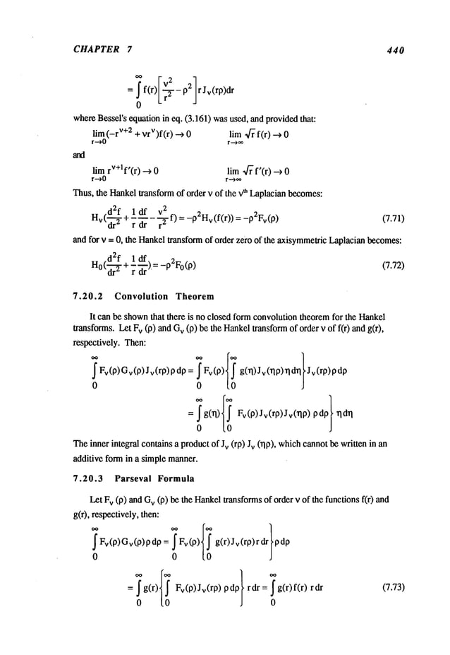
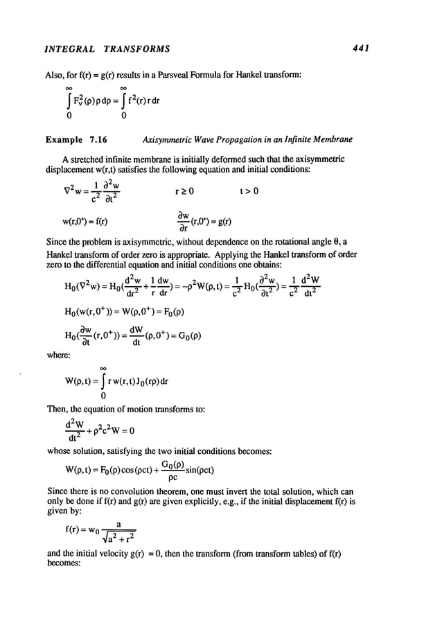
![CHAPTER 7 442
~r
dr =
e-kP
Jo(rp)
0~r2+k
2 P
Thus,the transformof the initial displacementfield is givenby:
a -a
Fo(p) = o - e pan d Go (p) =
P
and, the transformof the displacementw(r,t) is given by the expression:
a -a
W(p,t) = 0 -e pcos(pct) = o a e -aPRe [e-ipct]
P P
Letting H(p,t) represent the complex
function in W(p,t):
H(p,t) = o ae-P(a+ict)
P
then its inverse Hankeltransformcan be written in an integral form:
h(r, t) =1 [H
(p, t) ] = wo
a~ e-p(a+ict)J0(rp) dp
0
Notingthat the inversion of the Hankeltransformof exp[kp]/pis given by:
ie
kp 1
"-~- Jo(rp) P dP= ~r2 +
then the inverse transform of H(p,t) becomes:
1
h(r, t) woa
4(a + ict) 2 + r
2
and the solution can be obtainedexplicitly:
w(r,t) = Re[h(r,t)] = a [14r2 +a2 - c2t211/2
42R L ~’:~
where:
R=(r2 + a2 _ c2t2)2 + 4a2c2t2](https://image.slidesharecdn.com/advancedmathematicalmethodsinscienceandengineering-hayek-230318001731-2b30ece5/85/advanced-mathematical-methods-in-science-and-engineering-hayek-pdf-455-638.jpg)
![INTEGRAL TRANSFORMS 443
PROBLEMS
Section 7.14
1. Find the Laplacetransform of the following functions using the various theoremsin
Section7.14 and withoutresorting to integrations:
(a) cos(at) (b) t sin (at)
(c) at cos(bt) (d) sin (at) sinh
(e) n e-at (f) cos (at) sinh
2. Obtain the Laplacetransform of the following functions:
(a)f(t/a) (b)uf(t/a)
(c) d~t[e-atf(t)] (d) d~t[t2f(t)])
(e) te-atf(t) (f) t d 2f
dt
2
d [ at df
(g) n fit/a) (h) ~- e ~-]
(i) 4[t f(t)] (j) sinh(at)
(k)
t t
~x f(x)dx (1) ~f(t- x)dx
0 0
3. Obtainthe Laplacetransform of the following periodic functions; wheref(t+T) -- f(t)
andfl(t) representsthe functiondefinedoverthe first period:
(a) fl(t) 0 < t < T
(b)f(t) Isin (at)l
{+:
0<t<T/2
(c) fl(t)=_
W/2<t<T
(d) fl(t) =t (r~- T =r~
1 0<t<T/2
(e) fl(t) -
0 T/2<t<T
i
0_<t<T/4
(f) f~(t) T/4<t<3T/4
3T/4<t<T](https://image.slidesharecdn.com/advancedmathematicalmethodsinscienceandengineering-hayek-230318001731-2b30ece5/85/advanced-mathematical-methods-in-science-and-engineering-hayek-pdf-456-638.jpg)
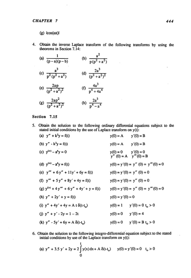
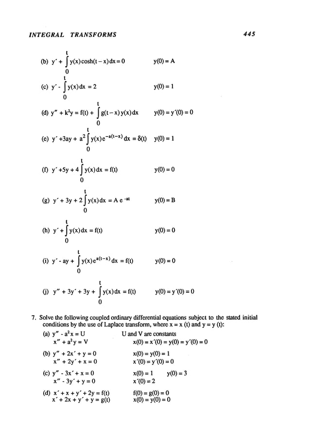
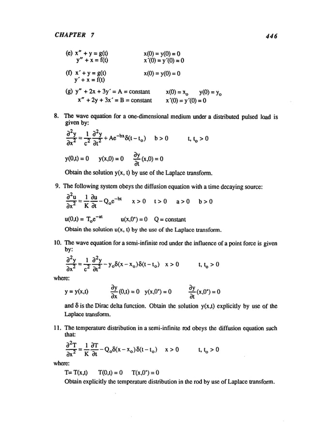
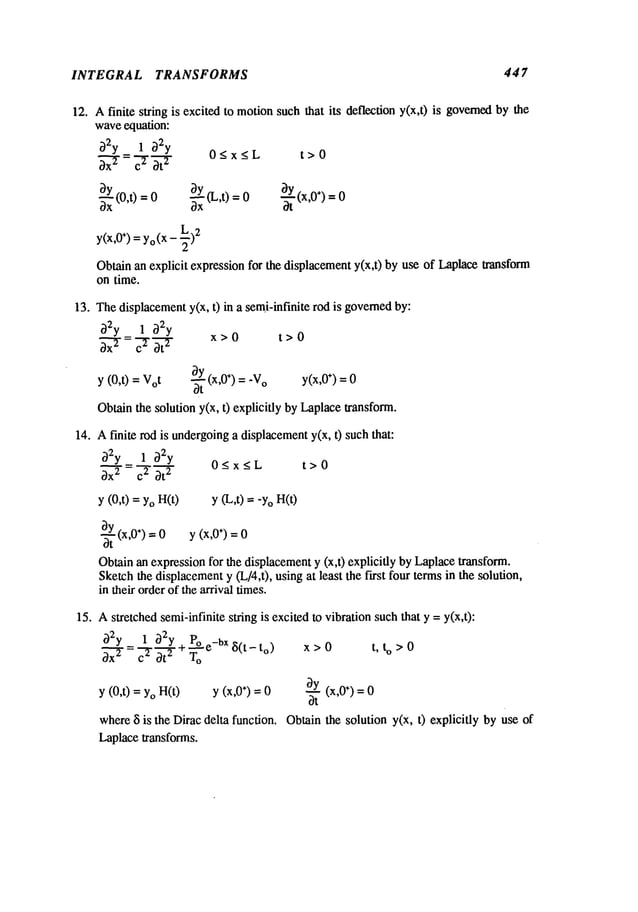
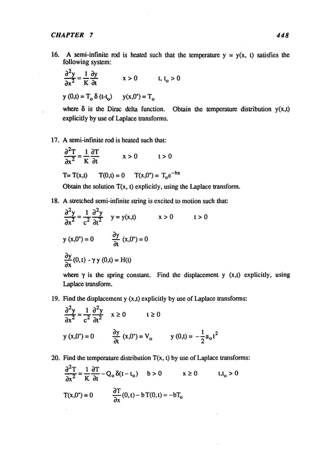
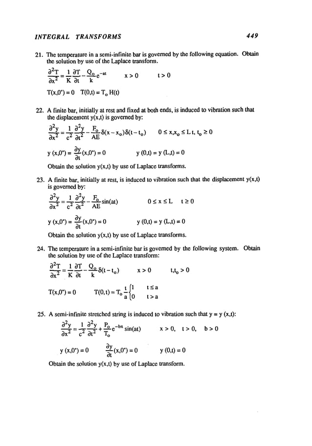
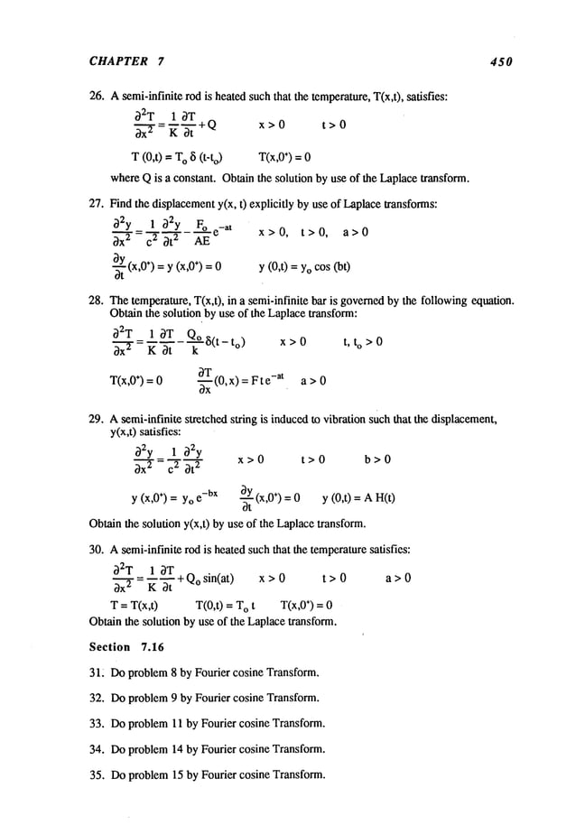
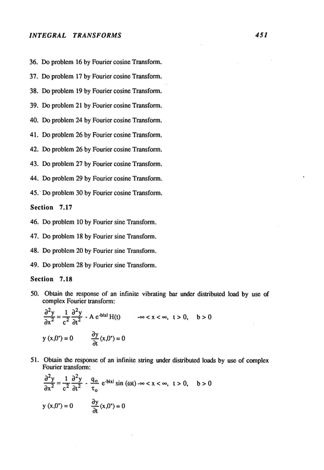
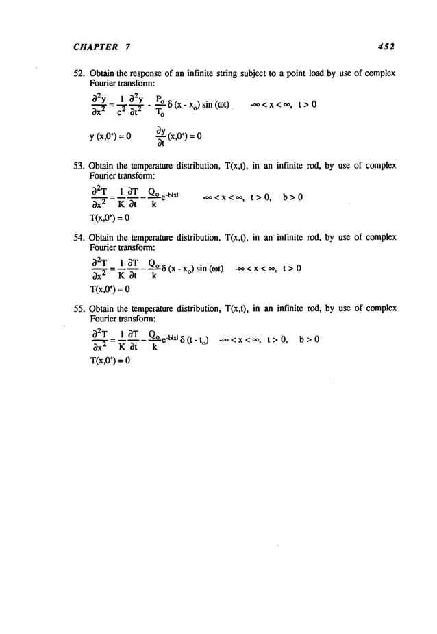
![CHAPTER 8 454
b
yp = ~ f(~) g(xl~) (8.5)
a
Substituting the particular solution ypin (8.5) in the boundaryconditions, onefinds that
they satisfy homogeneous
conditions; since the Green’sfunction g(xl~) satisfies the same:
Ui(Yp(X))=U i f(~)g(x~)d~ = f(~)Ui(g(xl~))d~=0
Thus,the total solution for the boundaryvalue problemposedin (8.1- 8.2) is:
y = Yh(X)
+ yp(X)
whereYh(X)
is the homogeneous
solution of the differential equations Ly= 0, and yp
the particular solution that satisfies the non-homogeneous
equation with homogeneous
boundarycondition. It follows that the homogeneous
solutions, with n independent
solutions {Yi(X)}satisfies the non-homogeneous
boundaryconditions (8.2).
Example $.1
Obtainthe total soludonfor the following system:
Ly=x2y"-2xy’+2y=l 1 < x < 2
y(1) = y’(2) =
The homogeneous
equation Ly=0yields the following two independent solutions:
Yl(X)= 2 y2(x)=
Toobtain
the
Green’s
function
for
this
system,
g(xl~)
satisfies:
Lg(x]~)
=2 T
-d2g(xl~) 2
x dg(xl~)d---T--+2g
(x[~) =~5
(x-~)
Toevaluate the Green’sfunction, let:
where:
Lgh(x~)
=
Lgp(xl~)
=8(x-~)
so that:
gh(xl~) = 2 + Bx
Toobtain the particular solution, one needsto resort to the methodof variation of the
parameters
(section 1.7), i.e.:](https://image.slidesharecdn.com/advancedmathematicalmethodsinscienceandengineering-hayek-230318001731-2b30ece5/85/advanced-mathematical-methods-in-science-and-engineering-hayek-pdf-467-638.jpg)
![GREEN’S FUNCTIONS 455
gp(Xl~)= vl(x)x2 + v2(x)x
so that the solution for a secondorder differential equationis givenby (1.26) as:
i q2x-TlX2 ~(TI-~) IX2 X 1
gp(Xl~)= ~-_’~ ~]~- drl= ~-f ~2’ H(x-~)
I
Thetotal Green’sfunction becomes:
Ixx ]
g(xl~)=Ax
2+Bx+ -~ ~2 H(x-~)
Satisfying the boundary
condition ong(xl~) results in:
A=-B- 3L~2 ~3J
and
the
Green’s
function
for
this
problem
isgiven
by:
It shouldbe notedthat this Green’sfunction is not symmetric,i.e. g(xl~)
~g(~lx).Using
the Green’sfunction, the particular solution yp(X)is:
2
= ~ g(x 1~)f(~)dE = ~(x2 -4x
yp(X) +3)
1
Notethat:
yp(1) = 0, and y~(2)
Thus,the total solution becomes:
Y = Yh+ Yp Yh= ClX2+ c2x
which upon satisfying the non-homogeneous
boundarygives:
Yh=(10x- 2) /3
y(x) = (-x2 + 16x+ 3) /
8.3 Green’s Function for an Adjoint System
Onecan developa Green’sfunction for the adjoint systemto a given boundaryvalue
problem.For the boundaryvalueproblem
in (8. I- 8.2), there exists an adjoint differential
operator Kgiven in (4.28) and the associated adjoint boundarycondition Vi(Y
) = 0 in
(4.36). Let the Green’sfunction for the adjoint systemg*(x[~) satisfy:
Kg*(x[~)= ~5(x-~) (8.6)](https://image.slidesharecdn.com/advancedmathematicalmethodsinscienceandengineering-hayek-230318001731-2b30ece5/85/advanced-mathematical-methods-in-science-and-engineering-hayek-pdf-468-638.jpg)
![CHAPTER 8 456
and satisfy the adjoint boundary
conditions:
V
i (g*(xIt) ) = 0 (8.7)
Theresulting adjoint Green’sfunction g*(xl~) is, in general, not symmetric
in (x,~).
Multiplying(8.6) by yp(X)and (8.1) by g*(xl~) and after subtracting the twoequations
integrating over the range (a,b), oneobtains:
b b
~(g*Lyp- ypKg*) dx = ~[g*(xl~ ) f(x)- yp(x) ~i(x- ~)]dx
a a
Theleft-hand side of (8.8) vanishesdueto the definition of an adjoint system(see section
4.12). Theright-hand side then gives:
b
yp(X) = ’f(~) g*(~x) (8.9)
a
Thus,the particular solution can also be obtainedas an integral over the source
distribution f(x) andthe adjoint Green’sfunctiong*(xl~).
Example 8.2
For the systemgiven in Example
8.1, obtain the adjoint Green’sfunction g*(xl~).
Theadjoint operator K:
K g’(xg)= x2g"" + 6xg" +6g*= ~5(x- ~)
and the adjoint boundaryconditions become:
g*0]~): 0 g*’(21~)+
2g*(21~)
Followinga similar method
of solution, one obtains the Green’sfunction g*(xl~) as:
g,(xl~) : ~(~2- 4~)(x.~_ + ¢~ ~z ~ H(x-~
It should
benoted
lhat g*(xl~) is not symmelric
in (×,~),
8.4 Symmetry of the Green’s Functions and Reciprocity
In general, both Green’sfunctions are not symmetricin (x,~). Howeve?r,
the Green’s
function g(xl~) andits adjoint formg*(xl~) are related. Rewritingthe twoolrdinary
differential equations(8.3) and(8.6)
L g(xl~) = 8(x-I) (8.3)
Kg*(xlrl) = ~(x-rl) (8.6)
multiplying(8.3) byg*(xlrl) and (8.6) by g(xl~), subtracting and integrating the resulting
twoequalities one obtains:](https://image.slidesharecdn.com/advancedmathematicalmethodsinscienceandengineering-hayek-230318001731-2b30ece5/85/advanced-mathematical-methods-in-science-and-engineering-hayek-pdf-469-638.jpg)
![GREEN’S FUNCTIONS 457
b b ,
a a
Theleft-hand side vanishesand the fight-handside gives:
g*C~lrl)=gCql~) (8.10)
This meansthat while the two Green’sfunctions are not symmelric,they are symmetric
with each other. This can be seen in Examples
8.1 and 8.2.
If the operator L is self-adjoint (see (4.34)), then L = Kand ) = Vi
(Y
). This
meansthat g*(xl~) = g(xl~) and hence:
g(xl~)= g(~lx) (8.11)
which meansthat Green’s function is symmetricin (x,~). This symmetryis known
the "Reciprocity"principle in physical systems. It indicates that the responseof a system
at x dueto a point sourceat ~ is equalto the responseat ~ due to a point sourceat x.
Example 8.3
If onerewrites the operator in Example
8.1 into a self-adjoint form~, (see section
4.11), one obtains:
d(1 dy~ 2
~y = ~xx t’~-~)+’~y =’~’-47 1 <x <2
Notethat the source function becomesf(x)=x-4. Defining~(x]¢) as the Green’sfunction
for the self-adjoint operator ~:
d(1 d~ 2_
o 0 ..
Followingthe methodused to find the Green’sfunction in.Examples8.1 and 8.2 results
in:
Notethat:
Theparticular solution is nowgiven by:
2
yp(X) = ~(x~) ~-~d~
1
whichis the sameas in Example
8.1.](https://image.slidesharecdn.com/advancedmathematicalmethodsinscienceandengineering-hayek-230318001731-2b30ece5/85/advanced-mathematical-methods-in-science-and-engineering-hayek-pdf-470-638.jpg)
![CHAPTER8 ’ 462
g(~’ ~): ~be(~)~t(x) (8.26)
It shouldbe notedthat the Green’sfunction in (8.26) is a symmetric
function in (x,~).
Thetotal solution is in the formof an infinite series resulting fromthe substitution of
(8.26) in the integral (8.21).
Example8.6 Green’sfunctionfor the vibrationof a finite string
FollowingExample
8.5, one can obtain the Green’sfunction for the stretched string
using eigenfunction expansion. Starting with the homogeneous
equation:
u" +~u= 0
u(O) = u(L) =
one can showthat the eigenfunctionsand eigenvaluesare:
d~n(X
) =sin(nrtx / L) n =1, 2 ....
~’n = n2 n2/L2 n=1, 2, ...
TheGreen’s function then becomes:
2 sin (nn x]L)sin (nn ~L)
n=l
8.8 Green’s Function for Semi-infinite One-Dimensional Media
TheGreen’sfunction for semi-infinite mediacannot be obtained through the methods
outlined in the previous sections. Essentially, the dependentvariables y(x) must
absolutely integrable over the semi-infinite region. Furthermore,boundary,value
problemsin a semi-infinite region have boundaryconditions on one end only. In such
problems,use of integral transformssuch as Fourier transforms becomes
necessary.
Thereis no general method
of solution, as each problem
requires the use of a specific
transformtailored for that problem.
Example
8.7 Green’sfunction for the longitudinal vibration of a semi-infinite bar
Obtainthe responseof a semi-infinite bar vibrating in longitudinal mode.Thebar is
excited to vibration bya distributed harmonic
force f(x)e-i°~t, wheref(x) is bounded
and
absolutely integrable. Thelongitudinal displacementof the bar y(x)e
"imt obeysthe
followingequation (see section 4.3):
~ f(x)
daY - k2y = -’~
x > 0
- dx
2
y(O):O 2:017¢2 C:~](https://image.slidesharecdn.com/advancedmathematicalmethodsinscienceandengineering-hayek-230318001731-2b30ece5/85/advanced-mathematical-methods-in-science-and-engineering-hayek-pdf-475-638.jpg)
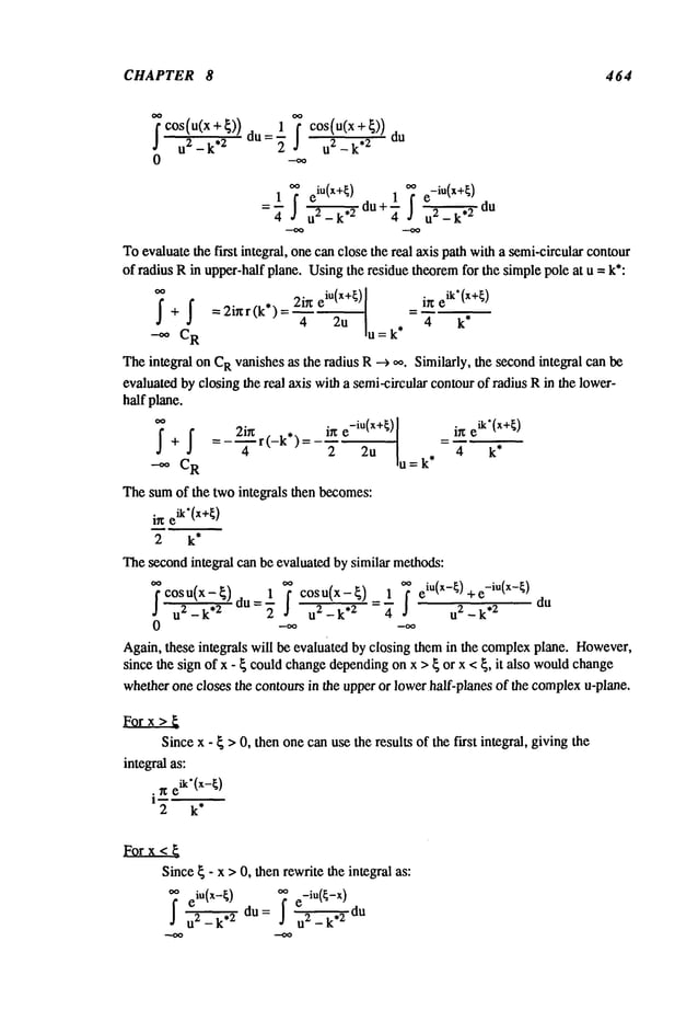
![GREEN’S FUNCTIONS 465
resulting in the integral as:
ine
ik’(~-x)
2 k*
Finally, assemblingthe twointegrals, one obtains the Green’sfunction for x > { or
x <{. Letting~l ---> 0, k*--> k, results in the final solutionfor g(xl{):
[i [eik(~+x) eik(~-x)]=_e~.~sin(kx
)
x<~
_~’L -
g(x 19)- | i Feik(~+x) eik(x-~)l ikx
[~" k -J = - T sin (k~) x >
Notethat the Green’sfunction g(xl~) -i~t represents only outgoing w
aves in t he farfield,
x > ~ but has a standing wavefor 0 < x < ~. Theresponseof the bar to a distributed load
is the integral of the Green’sfunction convolved
with the source term, i.e.:
y(x):f g,xlL
AE
d~=+._ e~’Xf
f(~)sin(k~)d~ + sin(kx) ik~ f(~)d~
0 Av~[ 0 x
8.9 Green’s Function for Infinite One-Dimensional Media
For infinite media, one mustapply Fourier Complex
transform. In this case, the
dependent
variable and all its derivatives up to (2n-l) mustdecayat somerate.
Furthermore,the source distribution mustbe absolutely integrable.
Example
8.8 Green’s function for the vibration in an infinite string
Obtainthe displacementfield of an infinite vibrating stretched string undergoing
forcedvibration due to a distributed time-harmonic
load f(x) -i°x. Since the string i s
infinite in extent, there are no boundaryconditionsto satisfy. For this problem,Fourier
Complex
transform is an ideal transform. Theequation of motionof the string (section
4.2) is givenas:
f(x)
d2y
k2y=~ -oo<x<oo
dx
2 T
O
TheGreen’sfunctionsatisfies the differential equation:
-
d2~g- k2g: ~(x - ~)
dx
2
Applyingthe Fourier Complex
transform (see section 7.17) to the differential equation
the independentvariable x, one obtains:
u2g
* _ k2g
* = e-iU~
where:](https://image.slidesharecdn.com/advancedmathematicalmethodsinscienceandengineering-hayek-230318001731-2b30ece5/85/advanced-mathematical-methods-in-science-and-engineering-hayek-pdf-478-638.jpg)
![CHAPTER 8 466
solving for g*, one gets:
e -iu~
g*(u) = u2 _
TheGreen’sfunction is evaluated fromthe inverse transformof g*(u):
1 ~ ¯ 1 ~e
iu (x -~)
g(xl~)= ~-~g*(u)e+mX du = 2"- ~" u2 _k~du
Dependingon whetherx > ~ or x < ~, one mayclose the path on the real axis with a
circular contourin the upper/lowerhalf planes of the complex
u-plane. In order to avoid
the creation of reflected wavesfromthe farfield regionx --> +,,0, onemustagainadd a
limiting absorption tothe material constants, as wasdone in Example8.7. Thus, the
Green’s function written for k = k* becomes:
1 ~ e
iu(x-~)
g(xl~)=~’n
-u2- k du
For x < ~, closure is madein the lower-halfplane, resulting in Green’sfunction, after
makingk* --> k, as:
g(xl
) x<
2k
For x >~, the closure is performedin the upper-halfplane, resulting in a Green’s
function of:
g(xl~
)~---""-~) x
= 2k
eik(x > ~
TheGreen’sfunction for the different regions can be written in one compactformas:
g(xl
):2k
Notethat the Green’sfunction represents outgoingwavesin the farfield x -->
Thedisplacementfield dueto a sourcedistribution f(x) as:
1 i
e_ik~ eik¢ f(~)
y(x) = ~ g(x]~ d~ = -- e
ikx f(~) d~ + -ikx
2r~kT
o
8.10 Green’s Function for Partial Differential Equations
Theuse of Green’sfunction for partial differential equationsparallels the treatmentgiven
to ordinarydifferential equations. Thereare, however,somedifferences that needto be](https://image.slidesharecdn.com/advancedmathematicalmethodsinscienceandengineering-hayek-230318001731-2b30ece5/85/advanced-mathematical-methods-in-science-and-engineering-hayek-pdf-479-638.jpg)
![GREEN’S FUNCTIONS 467
clarified. Thefirst beingthe definition of a self-adjoint operator. Let the linear partial
differential operatorL be definedas (see section D.7):
LOp(x)= ~ ak(x) k O
p(x) (8.27)
Ikl
<-
n
wherex is an m
th dimensionalindependentvariable and n is the highest order partial
derivative of the operator L. Theadjoint operator Kthen is definedas:
KOp(x)=2 (--1)lkl0k[ak(X)Op(X)] (8.28)
Ikl-<
n
If K= L, then Lis self-adjoint.
Example 8.9
TheLaplacianoperator V
2 in cartesian coordinates in three dimensions:
V2~l/ 02x 0y2 + 0z--~--
andis self-adjoint, since ak are constants. TheLaplacianoperator in cylindrical
coordinates
(r,0,z) written as:
L ~t = V2~t = --q-7~ + --- + ~_-X-~- +
--
Dr r Dr az r 2 202
is not self-adjoint, since the adjoint operator Kis givenby:
K~= 02~ 10~ 1 02~ 1
0r2 r DrI- r-T ~l/+ Oz-’--~- +r2 202
andis not equalto L.
However,
if one modifies L such that:
021~/ . 3~ r 02/1t + 1
gtl/=rL/l~=ro--~+-~-r + ~ r 202
then K= L, i.e. the operator ~is self-adjoint.
Forthe general partial differential equation,one canshow
that:
v(x) L u(x) - u(x) Kv(x) = V-~(u, (8.29)
whereVis the gradient in n-dimensional
Spacedefined by:
V= ~1 ~X
1
+ ~2 ~ + "’" + ~n OX
n
(8.30)
P is a hi-linear formof u andv, and ~j are the unit basevectors. Integrating the two
sides of (8.29) over the volume:
IR(VLu-uKv)dX=IRV.~dX=Is ~.~dS (8.31)
wherefi is the outwardnormalto the surface enclosing the region R. Thelast integral
transformationis the divergencetheoremstated as:](https://image.slidesharecdn.com/advancedmathematicalmethodsinscienceandengineering-hayek-230318001731-2b30ece5/85/advanced-mathematical-methods-in-science-and-engineering-hayek-pdf-480-638.jpg)
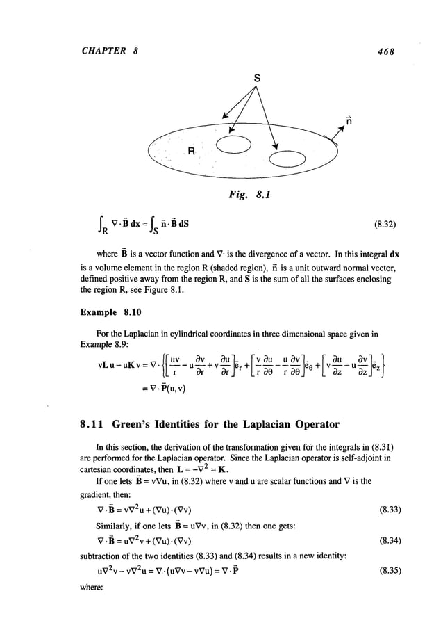
![GREEN’S FUNCTIONS 469
is a bi-linear function of u and v. Integrating eq. (8.35) over the volume
~R (vV2u-u VT-v) dx= ~R V. ~ dx= ~Sft. ~ dS
(8.37)
wherethe last integral resulted fromthe use of the divergencetheorem.
Thelast integral can be simplifiedto:
¯ Is~(’~vu-
~Vv)ds
:.}’s~~u
~v~
resulting in the identity:
l,~g-ug)dS (8.38)
Theterms in the integral overthe surface S represent boundary
conditions.
8.12 Green’s Identity for the Helmholtz Operator
TheHelmholtzequation has an operator given as:
L = -V2 - k
so that it is also self-adjoint, since the Laplacianis a self-adjoint operator. Substituting
for V
2 in eq. (8.35) by L abovethen:
v(-L - k)u - u(-L - k)v = uLv - vLu=
TheGreen’sidentity for this operator becomes:
~R (uLv- vLu) dx = ~S (u~- v~UnU) (8.39)
Theterms in the integral over the surface S represent boundaryconditions.
8.13 Green’s Identity for Bi-Laplacian Operator
Thebi-Laplacianoperator V
4 is definedas:
L = -V4 = -V2V
2
whichis a self-adjoint operator and showsup in the theoryof elastic plates. In order to
use the results for the Green’sidentity for the Laplacian,let V2u
= Uand V~v= V, then:
uLv - vLu = v~74u - u~74v = vV2U - uV2V
--[V.(vVU)-
Vv.
vu]-
[V.(uVV)-
Vu.
Rewritingthe terms in the secondbracketedquantities:](https://image.slidesharecdn.com/advancedmathematicalmethodsinscienceandengineering-hayek-230318001731-2b30ece5/85/advanced-mathematical-methods-in-science-and-engineering-hayek-pdf-482-638.jpg)
![CHAPTER 8 470
_- 4]-
then the Green’sidentity for the bi-Laplaciancanbe written as:
VV4U- uvav = V" {VV(V2U) - UV(V2V) + VU(V2V) - VV(V2U)} (8.40)
Integratiffg eq. (8.40) overthe volume
fR (VV4u-uV4v) dX= fR V’~dX = fs fi’~dS
O(V2u) uO(V2V)+V2vOU-v2uOV]ds
(8.41)
Thete~s in the integral over the surface S represent boundaryconditions.
Similarly, if one has a bi-LaplacianHelmholtz
type operator, i.e. if L =- V~+ ~,
then:
=~s[ ~n -"~*vv~-v u~].~ (8.4~)
8.14 Green’s Identity for the Diffusion Operator
Forthe diffusion equation,the operatorandits adjoint are definedas:
~) ~ KV
2
(8.43)
L = ~- - KV2 and K = - ~- -
Thus,these operators give the followingidentity:
( o3U ~V) K(VV2U_DV2V)
vLu- uKv: ~v-~- + u -~-)
= 3-~ uv - KV"(vVu - uVv) (8.44)
Hereweare dealing in four dimensionalspace, i.e. (x,y,z and t). In this space one
defines a newgradient Vas:
-" 0 g +~ (8.45)
where~’ is the spatial gradient definedin (8.30) and ~t is a unit temporalbasevector
time, orthogonalto the spatifil unit base vectors. Usingthe newgradient, one can rewrite
(8.44) as:
vLu- uKv= V- P(u, v) (8.46)
where~(u, v) is definedas:
~ = UV~t-- K(V~’U--
U~V
)
(8.47)](https://image.slidesharecdn.com/advancedmathematicalmethodsinscienceandengineering-hayek-230318001731-2b30ece5/85/advanced-mathematical-methods-in-science-and-engineering-hayek-pdf-483-638.jpg)
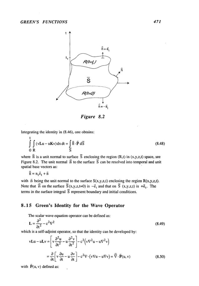
![CHAPTER 8 472
and the gradient Vgivenin (8.45). Integrating the identity (8.50) overthe spatial region
Rand time, one obtains:
t t
~ f(vLu-uLv)dx dt ~f ~’~’dxdt=j~’~d~ (8.52)
OR OR S
Theterms in the surface integral over ~ has both initial and boundaryconditions.
8.16 Green’s Function for Unbounded
Media--Fundamental
Solution
Considerthe followingsystemon the independentvariable u(x):
Lu(x) = f(x) x in R
n (8.53)
whereL is an operator in n-dimensional
space and f(x) is the source termthat
absolutely integrable over the unbounded
region R
n. Definethe Green’sfunction g(x]~)
for the unboundedregion, knownas the Fundamental
solution, and the Green’s function
g* (~) for the adjoint operator Kto satisfy:
Lg(x[~):
6(x- (8.54)
K (8.55)
whereg(xl~) and g*(xl~
) mustdecayin the farfield at a prescribed manner.It shouldbe
noted that g* (~)= g(~x). Multiplying (8.53)by ) and (8 .55) by u(x) and
integrating over the unbounded
region, one obtains:
~R
n (uKg*-g’Lu)dx : n [u(x) 6( x-~)- g* (x~) fix
= u(~)- fR g~ (~) f(x)dx
n
Theintegral onthe left-hand side can be written as a surface integral, see (8.31), overthe
surface Sn. Thesurface Sn of an unbounded
medium
could be taken as a large spherical
surface with a radius R--> ~. Theintegrand then mustdecaywith Rat a rate that would
makethe integral vanish. Thecondition ong(xl~) wouldalso require that it decaysat a
prescribedrate as R--~ ~. Thus,if the left-hand side of(8.31) vanishes, then:
u(~): ~Rn g*(x[~) f(x) dx = ~Rn g(~Jx)f(x)dx
Changing
x by ~ and vice versa, one can write the solution for u(x) as:
u(x):-alan g(r~) f(~)d~ (8.56)](https://image.slidesharecdn.com/advancedmathematicalmethodsinscienceandengineering-hayek-230318001731-2b30ece5/85/advanced-mathematical-methods-in-science-and-engineering-hayek-pdf-485-638.jpg)
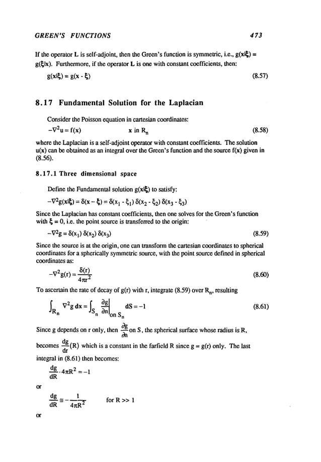
![CHAPTER 8 4 74
1
g(R) for R >> 1 (8.<62)
4/~R
This meansthat the Green’sfunction for an unbounded
three dimensionalregion
mustdecayas I/R. Returningto eq. (8.60), one can integrate the differential equation
directly bywriting the Laplacianin spherical coordinatesin r only, i.e.:
r2 dr
= 4~1.2 (8.63)
Direct integration results in:
g(r) = ~ +C
since g(R) for R>>1 must decayas l/R, then -- 0, giving:
1 1
+4+
4]
I I
g(x-~)- 4,~[(Xl _~1)2 +(x2_~2)2 +(x3_F~3)2]1/2 =4~[x-~ (8.64)
8.17.2 Two dimensional space
In twodimensionalspace, the Green’sfunction satisfies:
-v2g(xlg)
=8(x-g)=8(xl- ~1) ~i(x2 -~2) (8.6:5)
Asthe twodimensionalLaplacianhas constant coefficients, one can shift the source to
the origin:
-V2g = (5(Xl) (5(x2)
Sincethe sourceis at the origin, then onecan transform(8.66) to cylindrical coordinate
two dimensionalspace and the Green’sfunction becomesg(r):
-V2g
=- 1,d--- (r d-d~g
/ =8(’-~) (8.67)
rork ur,~ 2rcr
Again,to define the behaviorof g(r) as r --) oo, onecan integrate (8.66) over
unboundedregion Rn:
fR V2gdx=/s ~-~n g dS-=-’~
(R)’2nR=-I
n n on S
n
so that:
dg_ 1
dR - 2~R
or:.
1
g(R)_-- -~-~ logR for R >>1
Integrating (8.67) directly, oneobtains:
(8.68)](https://image.slidesharecdn.com/advancedmathematicalmethodsinscienceandengineering-hayek-230318001731-2b30ece5/85/advanced-mathematical-methods-in-science-and-engineering-hayek-pdf-487-638.jpg)
![GREEN’S FUNCTIONS 4 75
g(r) = -~ log r +
AgainCmustbe neglected in order that g(r) behavesas in (8.68), giving:
g(r)=-~n log r =- 2-~log[x ~ +x~]
g(x- ~)=- 2"-~ll°g[
(xl-~1)2
+(x2
- ~2)2]
1/2 =- 2"-~1
lo~x
- ~ (8.69)
8.17.3 One dimensional space
For the one dimensionalcase, g satisfies:
d2g = 8(x-~)
dx
2
Direct integration yields the fundamental
solution of:
1
g(xl~):- EIx- (8.70)
8.17.4 Development by construction
Onecan derive the Green’sfunction by construction, whichis yet another methodfor
development
of the Green’sfunction. First, enclose the source region at the origin by an
infinitesimal sphereR
e of radius ~. Starting with the definition of Green’sfunction:
-V2g= ~5(x) x in R
e
then, since the sourceregionis confinedto the origin:
V2g = 0 outside R
e
Rewritingthe Laplacianin terms of spherical coordinates, then:
1 d Ir2 dg
1
V2g = ~-~-[_ ~-j = 0 outside R
e
Bydirectly integrating the differential equationabove,oneobtains:
g=C~+c
2
r
Since g decaysas r --> 0%then C
2 -- 0. Integrating the equationover the infinitesimal
sphere Re:
-~Re V2gdX=~R,~ ~5(x)dx=l
0g
=-~R
e V "Vg dx = -~Se ~-nnlonSe
ds
0g]
el
= -~S~~rr = dS = e--2-- ~S
e dS= 4nC,](https://image.slidesharecdn.com/advancedmathematicalmethodsinscienceandengineering-hayek-230318001731-2b30ece5/85/advanced-mathematical-methods-in-science-and-engineering-hayek-pdf-488-638.jpg)
![CHAPTER 8 476
a a
where the normal derivative -- = q
On Or"
1
function g = ~.
4~r
1
= -- and the Green’s
The constant becomes C1 4g
8.17.5 Behavior for large R
Thebehaviorof u(x) as R -~ o~ can be postulated from(8.38). Theintegration
the surface of an infinitely large sphereof radius Rmustvanish. Thus:
fRn (uLg- gLu) dx = ~Sn(R_~ oo) (u ~ng - g ~-~)
where fi is the unit outwardnormaland -- = --. For three dimensional space,
On OR
1 Og 1
g = ~-, andOn
= R
2 so that the surface integral abovebecomes:
L. [-u(R) 0u(R) 1
lm /-~’~- + 4~R
2 --)
R-~L R OR
Thisrequiresthat thefunctionu andits derivativebehave
as:
u(R) + R d~RR)
1
R
p
p > 0 (8.71)
0g 1
-- _=-, so that the surface integral above
For two dimensional media, g = log r, On r
becomes:
Lim [u(R) + 0u_(R)-(logR)]2~R--)0
R ~ o~1_ R OR J
Thisrequires that the function u andits derivative behaveas:
u(R)+RlogR0_u~(_~R) 1
R
p
p > 0 (8.72)
8.18 Fundamental Solution for the Bi-Laplacian
Considerthe bi-Laplacian in two dimensionalspace:
-V4g= 8(x - ~) x in R
n (8.73)
then one canagain shift the source to the origin, since the bi-Laplacianhas constant
coefficients.
-V4g= 8(x) = 8(Xl) 2) (8.74)
Rewritingthis equation in twodimensionalcylindrical coordinates:
[1 d f d .~-12
-V4g= -(V2)2g = - L’~ ~rr ~r ~rJj g=
Direct integration of (8.75) results in:
(8.75)](https://image.slidesharecdn.com/advancedmathematicalmethodsinscienceandengineering-hayek-230318001731-2b30ece5/85/advanced-mathematical-methods-in-science-and-engineering-hayek-pdf-489-638.jpg)
![GREEN’S FUNCTIONS 4 77
2
g = - ~ [log r - 1] + C1
r2 log r + C2
r2 + C
3
Integrating equation (8.74) over Largecircular area n w
ith R>>
1, one
obtains the
conditionthat as R-->
_= - ~ log R R >>
V2g 1
This requires that all the arbitrary constants C
1, C
2 and C
3 vanish, giving g as:
r
2
g =~--~ [1- logr] (8.76)
8.19 Fundamental Solution for the Helmholtz Operator
Consider the Helmholtzequation:
-V2u - ~u = f(x) x in n (8.77)
whereL = -V
2 - ~, is a self-adjoint operator. TheGreen’sfunction satisfies the Helmholtz
equation:
-V2g- ~,g = ~i(x - ~) (8.78)
Since the operator has constant coefficients, then onceagain, the sourcecould be
transformedto the origin. Thesolution for u(x) can be obtained as an integral over the
sourceterm fix) and the Green’sfunction, as in (8.56).
8.19.1 Three dimensional space
Todevelopthe Green’sfunction by construction, enclose the source at the origin by
an infinitesimal sphereRe, such that:
-V2g- kg = 0 outside R
e
Replacingk by k2 and writing the equation in spherical coordinates one obtains a
homogeneous
equation:
r-~ d It2 dgl+ k2g =
0 outside R
e
~L ~J
whichhas the solution:
eikr e-ikr
g = CI --~ + C2 ~ (8.79)
r
with e-i°a assumedfor the time dependence
leading to the Helmholtz
equation, the two
solutions represent outgoing and incomingwaves, respectively. For outgoingwaves, let
C
2 -- 0. Integrating (8.78) withthe source at the origin overRe:
-f-e’sR V2g dx- k2fg dx = 1 (8.80)
.~Ra](https://image.slidesharecdn.com/advancedmathematicalmethodsinscienceandengineering-hayek-230318001731-2b30ece5/85/advanced-mathematical-methods-in-science-and-engineering-hayek-pdf-490-638.jpg)
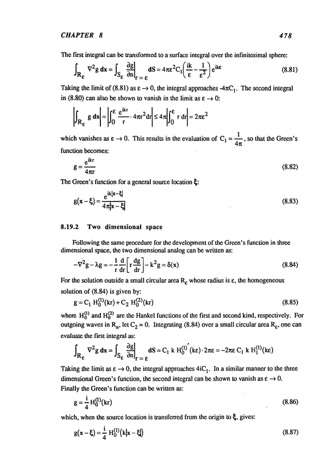
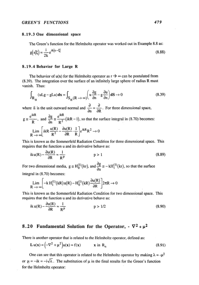
![CHAPTER 8 480
(-v
2 +~2)g(xl~)=~(x-)
results in the followingGreen’sfunction.
8.20.1 Three dimensional space
Substitution of ~t in (8.82) gives:
e-tXr
g(r) =
4~zr
(8.92)
(8.93)
8.20.2 Two dimensional space
Substitution of ~ in (8.86) results in:
g= H(o1)(igr) = ~-~ Ko(gr)
whereK
o is the modifiedBesselfunction of the first kind.
8.20.3 One dimensional space
as:
(8.94)
Substitution of p. in (8.88) results in the Green’sfunction for one dimensionalmedia
e-~,lxl
g = ~ (8.95)
2l.t
8.21 Causal Fundamental Solution for the Diffusion Operator
For the diffusion operator:
~)u
K~72U
= f(x, t) x in R
n, t > 0
3t
the Green’sfunction satisfies the followingsystem:
3g ~V2g= ~(x_ ~) 8(t_,c)
Ot
where:
g =g(x,t[~,
satisfies the initial conditiong(x,O+]~,x)
= O,and satisfies the causality condition:
g=O for t<’c
whichstates that the solution is null until t =x. Sincethe diffusion operator has
constant coefficients, one canshift the ~ andx to the origin
g = g(x,@,O)= g(x,t)
satisfying the diffusion operator:
(8.96)
(8.97)](https://image.slidesharecdn.com/advancedmathematicalmethodsinscienceandengineering-hayek-230318001731-2b30ece5/85/advanced-mathematical-methods-in-science-and-engineering-hayek-pdf-493-638.jpg)
![GREEN’S FUNCTIONS 481
bg ~:V2g= ~5(x) ~i(t)
(8.98)
~t
with the causality condition nowgiven by:
g=0 t<0
In order to obtain the Fundamental
solution, one can apply the Laplacetransform on
time. Usingthe definitions and operations of Laplacetransformin section (7.14) and
defining the Laplacetransform:
Lg(x,t) = ~(x,p)
the differential equation(8.98) transformsto:
_V2~+ p ~ = ~(x) (8.99)
K K
Equation(8.99) resembleseq. (8.92) with solutions for three and two dimensionalmedia
with g2 = P.
K
8.21.1 Three dimensional space
Withkt = ~-, the transform of the Green’sfunction for three dimensionalspacein
(8.93) gives:
-r p4-~7~
g(r,p) =
4nKr
whoseLaplaceinverse transform gives:
e-r2/(4~t)
g(r,t) = (4rtKt)3/2 (8.100)
Rewriting(8.100) to revert to the sourcespace and time { and x gives:
e-lX-~21
[4K(t-~’)]
g(x -- ~ [ -- ~]~)
~
t (~)J i_4.~i:~.t __ ~.13/2 H~(t -- ~I~) (8.101)
note that the resulting expressionfor g is causal.
8.21.2 Two dimensional space
Thetransform of the Green’sfunction in two dimensionalspace given in (8.92), with
g = ~/~ is:
~(r, p)=2-~K
Ko
(r p~/-P--7~
)
has an inverse Laplacetransformof:
1 r2/(4Kt)
g(r, t) = --e- H(t) (8.102)
4~xKt](https://image.slidesharecdn.com/advancedmathematicalmethodsinscienceandengineering-hayek-230318001731-2b30ece5/85/advanced-mathematical-methods-in-science-and-engineering-hayek-pdf-494-638.jpg)
![CHAPTER 8 482
which,upontransformingthe coordinates to the source location and time results in the
following expression:
1 e-lx-~l
2/[4~¢(t-g)]
H(t - X)
(8.103)
g(x -~,t- X) = [4r~(t-
8.21.3 One dimensional space
with It = ~-~, the transform of the Green’sfunction for one dimensionalmedium
can be written as (see (8.95)):
~(x,p) : 2 .~~ (8.104)
Theinverse Laplacetransform of (8.104) can be shownto have the form:
1 e-x2/(4~a) H(t)
(8.105)
g(x,t)
andtransformingthe origin to the actual location:
1
g(x - ~, t - x) = [4r~(t z)1/2 e-(X-~)~/[4~(t-x)] H(t (8.106)
Definingthe Green’sfunction g* (x]~) for the adjoint operator Kas:
3g* ,-.2 ¯
K g* = --~- - ~v g = ~(~ - ~) ~(t -
and using the form(8.56), one can write down
the solution for u(x,t)
u(x,t)= ~ ~ g(x,t[~,z)f(~,x)d~dx (8.107)
0 R
n
8.22 Causal FundamentalSolution for
Forthe waveoperator, the solution u(x) satisfies:
~’~- C2~
72 U(X,t) = f(x,t)
X in Rn,
and the Green’sfunction then satisfies:
satisfying the homogeneous
initial conditions:
g(x,O+l~,x)= and ~ (x,O+l~,x) =
dt
the WaveOperator
t>0 (8.108)
(8.109)](https://image.slidesharecdn.com/advancedmathematicalmethodsinscienceandengineering-hayek-230318001731-2b30ece5/85/advanced-mathematical-methods-in-science-and-engineering-hayek-pdf-495-638.jpg)
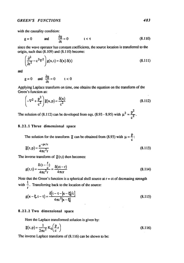
![CHAPTER 8 ~484
J
Notethat the Green’sfunction has a trail that decayswithct at any fixed position r with a
sharpwavefrontat ct = r. TheGreen’sfunction can be transferred to the location of the
sourceto give the Green’sfunction as:
Htc{t-x)-Ix-~] 1/a H(t-x) (8.118)
g(x - ~’t- x) = 2r~C[Ca(t_x)z _[x ]
8.22.3 One dimensional space
For the one dimensional medium:
e-plxl/e
~(x,p) = (8.119)
2pc
whichmaybe inverted by Laplacetransform to give:
g(x,t) H[
t- ~x[/c] n(t) (8.120)
2c
Notethat the Green’sfunction is constant, but has twosharp wavefrontsat x = _ct.
Upon
transferring to the location of the source, one obtains:
g(x- ~,t- %)=H[t- x- Ix ~- ~[/c] H(t- %) (8.12I)
2c
Since the waveoperator is self-adjoint, then the solution u(x,t) canbe written from(8.56)
as."
u(x,t)= ~ f g(x,~,%)f(~,%)d~d%
0 R
n
8.23 Fundamental Solutions for the Bi-Laplacian Helmhoitz
Operator
Thefundamentalsolution for the Bi-LaplacianHelmholtzoperator applies to the
vibration of elastic plates. Since the plate is a twodimensionalmedium,
then the
Fundamental
solution satisfies the followingequation:
(-~ 74 + k4)g(x[~) = 8(x- ~) x n (8. 122)
Sincethe operator has constant coefficients, then one can transformthe source location to
the origin andwrite out the operatorin cylindrical coordinatesin the radial distance:
(_V4
+k4)g(r) =8(r_==~) (8.123>
2~r](https://image.slidesharecdn.com/advancedmathematicalmethodsinscienceandengineering-hayek-230318001731-2b30ece5/85/advanced-mathematical-methods-in-science-and-engineering-hayek-pdf-497-638.jpg)
![GREEN’S FUNCTIONS 485
Toobtain the solution for g(r), one can apply the Hankeltransformon r, see Section
7.19, wherethe Hankeltransformof g(r) is g(p):
1
resulting in the solution:
Theinverse Hankeltransform of ~(p) can be shownto be:
-1 o~ J0(rp)
(8.124)
g(r) = ~ j" p
¯ 0 p4_ k
4
In order to performthe integration in the complex
plane, one needsto extendthe
integration onp to (.~o). Usingthe identities (3.38) and(3.39), one cansubstitute
byH(o
1) andH(o
2) as:
g(r): _~1~ P[H(01)(rP)_
+ I-I(0~)(rP)]
4~ J p4 _ k
4
0
SinceH(0:Z)(rp)=-H(01)(-rp), the integral in (8.125) canbe extendedto _oo
g(r) =-~n ,, p4 _ k 4 dp (8.125)
Since H(ol)(x) behavesas eiX/~
- for x >>1, then one can close the contour in the upper
half-plane. Theintegrand has four simple poles, tworeal and two imaginary. Usingthe
principle of limiting absorption then the four simplepoles wouldrotate counterclockwise
byan angleequal to the infinitesimal damping
coefficient rl, suchthat k* = k(1 + irl).
Thetwosimplepoles that fall in the upper-half plane are k* and ik*. Thefinal solution
for g(r) becomes
the sumof tworesidues after letting k* --~
g(r) = - 8-~ [H(01)(kr) - H(ol)(ikr)] (8.126)
TheI-lankel function.of an imaginaryargumentca~ be replaced by -2iKo(kr)/~, so that the
final expressionfor the Fundamental
solution is written as:
g(r)=- 8k-~ [iH(01) (kr) - n2-. K0 (kr)]
8.24 Green’s Function for the Laplacian Operator for
Bounded Media
In this section, the Green’sfunction is developedfor bounded
mediafor the Laplacian
operator. This is accomplishedthrough the surface integrals that weredevelopedwhenthe](https://image.slidesharecdn.com/advancedmathematicalmethodsinscienceandengineering-hayek-230318001731-2b30ece5/85/advanced-mathematical-methods-in-science-and-engineering-hayek-pdf-498-638.jpg)
![CHAPTER 8 486
Green’s
identifies were
derivedearlier. Forthe Laplacian
operator,start withtheGreen’s
identityin eq. (8.38)andthe differentialequation
(8.58). Letv=g(xl~)
in (8.38)
from(8.58), oneobtainsthe following:
3u
IR[-g(x~)f(x) + u~i(x-~)] dx = Is[g~n- u
which,uponrearrangement
gives:
IRg(xl
f(x)dx
+
is jdSx
Since
the
Laplacian
isaself-adjoint
operator,
then
one
can
change
the
independent
variable
xto~and
vice
versa,
giving:
u(x)= IRg(xl~)f(~ ) d~+IS~ [g(x,~) ~-~ ) ~n~ dS[ (8. 128)
Thissolutionis composed
of twointegrals.The
first is a volume
integraloverthe
volume
source
distribution.
The
second
is a surface
integralthatrextuires
thespecification
of thefunction
u(x)and
thenormal
derivative
~u(x)l~n
at every
pointonthesurface.
Those
requirements
would
over-specify
the boundary
conditions.Onlyoneboundary
condition
canbeprescribed
at every
pointof ihesurface
for a unique
solution.Toadjust
thesurface
integrals
sothatonlyone
boundary
condition
ne~ds
to bespecifi¢xl
at each
pointof thesurface,
anau×iliary
function
~is defined
such
ihat:
-VB~(xl~) : 0 x in R (8.129)
Substitutingv = ~(xl~
) in (8.38) oneobtains:
Again
switching
x to { andvice versa, oneobtainsa new
identity onthe auxiliary
funcfion:
DefiningG(xl~
) = g" ~ andsubtracfing(8.130)and(8.128)results in a newidentity:
a xl~~(~)
( )~n~ ]S~dS~ (8.131)
D~pending
onthe
prescribed
boundary
condition,
one
can
eliminate
one
ofthe
two
surface
integrals.](https://image.slidesharecdn.com/advancedmathematicalmethodsinscienceandengineering-hayek-230318001731-2b30ece5/85/advanced-mathematical-methods-in-science-and-engineering-hayek-pdf-499-638.jpg)
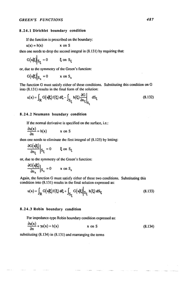
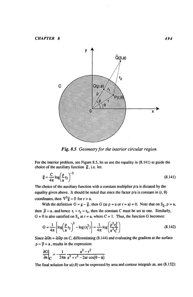
![GREEN’S FUNCTIONS 495
Fig. 8.6 Geometry for the exterior circular region
a 2~ r
47zu(r,O):.-f f log~ arll f(p,~)pdpd0
~ pr2)
00
÷2(a2 _ r2) 2~r h(0) a
(8.143)
"£ J r 2 +a2"-_~-a~-os(0_0)
0
ThesameGreen’sfunction can be obtained by the use of imagesources and by
requiring the Green’sfunction satisfy the boundaryconditions. Starting with:
~ =~ logr22 -~D(r,4np)
where V2D
= 0, and solving the homogeneous
equation on Dresults in: D = E(p) log r
F(O). Theconstant Cas well as the functions E(O)and F(p) will be evaluated through
satisfaction of the boundary
conditionsat r =a or p = a.
=g-~= _~1 {logrl 2 + Clogr22+ E(o)logr + F(p)}
G
Glp= ~ = a : 0 = - 4--~-{logro2+ Clogro
2 + E(a)logr+ F(a)}
Thus,C= -1, E(a)= 0 andF(a)
G]r =a : 0 = -~-~ {logrl 2 (a)- log r22 (a)+ E(p)loga+ F(p)}](https://image.slidesharecdn.com/advancedmathematicalmethodsinscienceandengineering-hayek-230318001731-2b30ece5/85/advanced-mathematical-methods-in-science-and-engineering-hayek-pdf-502-638.jpg)
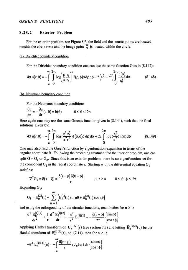
![CHAPTER 8 500
E(nl)(2)(u)_ Jn(PU)#sin(n~)~
- gU2 [cos(n~)J
n> 1
TheinverseHankel
transformof nth order gives:
1 ~sin (nqS)~(r/ n r<p
E(nl)<2)(r)= ~ [cos(n~)J[(p n
r > p
ForE(o2)(r),seeeq. (8.69):
1
2rp cos(0-,)]
E(02)
(r) = _~.~log(rl)= 2
Finally,substitutingtheseexpressions
into theseries for GI:
1 log[r2 + p2 -2rp cos(0-,)]
O’(r’°lP’*)
=
cos(n(O- ¢))
+ "~"~ =1
for r < p (8.150)
1 log[r2 + p2 -2rp cos(O-~)]
G(r,01p,) =
for r > p (8.151)
+ 2rr cos(n(0 - ~))
n=l
For the solutionto the secondcomponent
G
2, onecan obtainthe solutionbyuse of the
solution of Laplace’seq. withNeumann
boundary
condition:
1 £ cos(n(0- @))
(8.152)
C2(r,01
)--
n=l
8.29 Green’s Function for Spherical Geometry for the
Laplacian
Fora three dimensional
regionhavinga sphericalboundary,
there are twoGreen’s
functions,onefor theinteriorandonefor theexteriorof thesphericalsurfaceat r = a, see
Figures8.7 and8.8.
TheLaplacian
operatorin three dimensional
spacein sphericalcoordinates
canbe
writtenas:
-V2u(r,0,~)
= f(r,0,~) interior r _<a, < 0 -<~, 0 _< ~ <
_ 2~r
exteriorr_>a, 0_<0_<r~, 0_<~_<2n
Thesourcepoint Q(p,~,~)has an imageat ~(~,~,~) such that ~ = a2/p,.
distances
r1,r2andr0 aregivenby:
rl2 = r2+ p2_2rpcos00](https://image.slidesharecdn.com/advancedmathematicalmethodsinscienceandengineering-hayek-230318001731-2b30ece5/85/advanced-mathematical-methods-in-science-and-engineering-hayek-pdf-507-638.jpg)
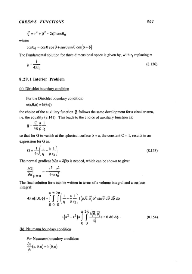
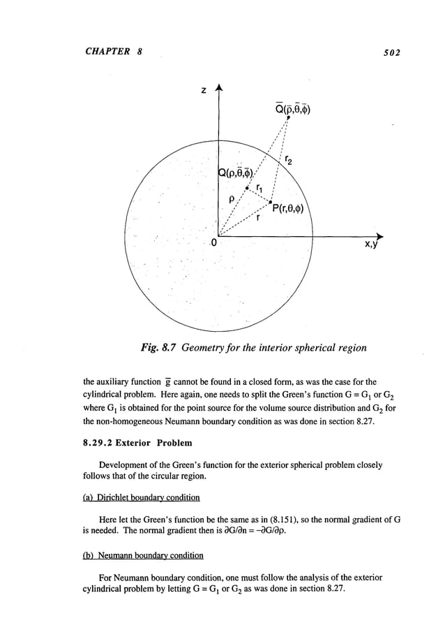
![GREEN’S FUNCTIONS 503
P(r,e,¢)
0
Fig. 8.8 Geometry for the exterior spherical region
8.30 Green’s Function for the HelmholtzOperatorfor
Bounded Media
Considerthe Helmholtzoperator in section 8.12. Substituting for u from(8.77) and
v = g from(8.78) into the equality in (8.39) results in the sameexpressiongiven
(8.128):
g(xl~)
8u(~)
- 8g(xl~)
]
u(x) = ~R g(x[~)f(~)d~ + ~S~
0n~ JS~
(8.128)
Following
the analysis undertakenfor the Laplacian,let the auxiliary function ~(
satisfy:
-V2~(xI~)- X~(x[~)= x in R (8.155)
Letting the Green’sfunction G for the boundedmediabe defined as G= g - ~, then the
final solution for the non-homogeneous
problemis the sameas the Laplacian’s, eqs.
(8.132-8.153).
8.31 Green’s Function for the HelmholtzOperatorfor Half-
Space
Refer to the geometryof three or twodimensionalhalf-spaces in section 8.26. For
twodimensionalspace, delete the coordinate y fromthree dimensionalsystem, such that
~:~ < X < o~, Z > 0.](https://image.slidesharecdn.com/advancedmathematicalmethodsinscienceandengineering-hayek-230318001731-2b30ece5/85/advanced-mathematical-methods-in-science-and-engineering-hayek-pdf-510-638.jpg)
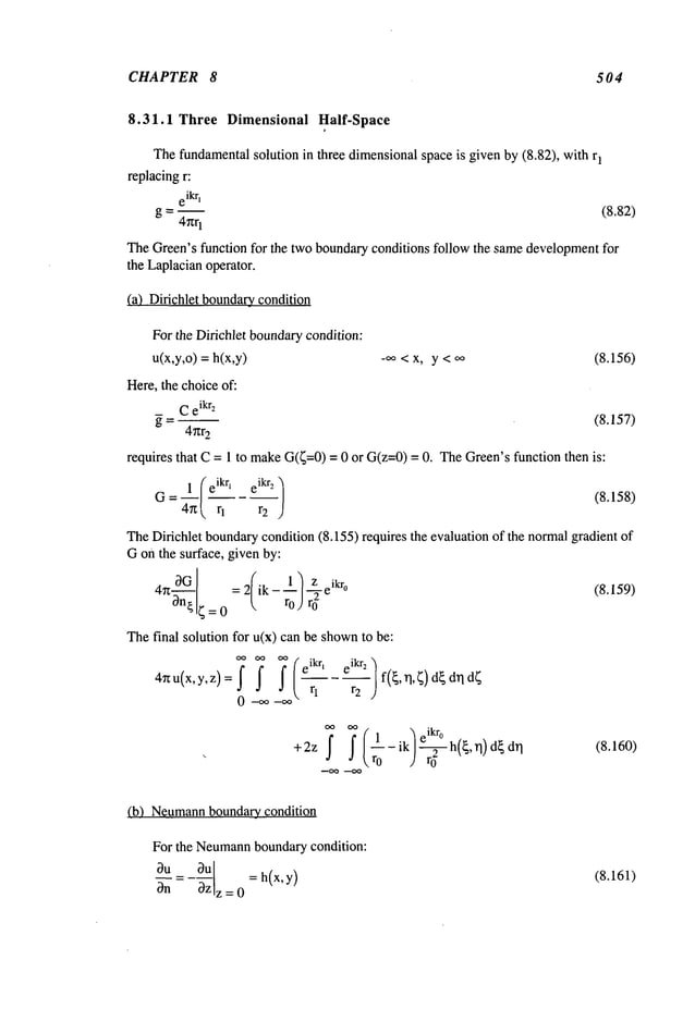
![GREEN’S FUNCTIONS 505
the Green’sfunction must satisfy 3Glen= -3G/~= 0 on the surface ~ = 0 or -3G/~z= 0
on the surface z = 0. It can be shown
that the constant C= -1, giving the Green’s
function as:
= ~1/eikr~ eikr2
G 47z~ q +--r
2
Thefinal solution for u(x,y,z) can be written as:
4rtu(x,y)=f ~ j" eikr’
-- + -- f ,~, d~d~d~
0 rl
+2 ~ h(~,n) d~ (8.163)
ro
(8.162)
8.31.2 Two Dimensional Half-Space
ThefundamentalGreen’sfunction for twodimensionalspace is given by, with r
1
replacingr:
g : ¼H(01)(krl) (8.86)
(a) Dirichlet boundarycondition
For the boundarycondition, one mustsatisfy G= 0 on ~ = 0 or z = 0, such that:
iC
~ = ~ Hgl) (kr2) (8.164)
so that C=1 resulting in the Green’sfunction as:
G= ¼[H(o£)(kq)
- H(o2)(kr2)] (8.165)
so that:
a or, = ot
30 iz H(1)[~
and the final solution can be shown
to havethe form:
0--~
--2Z ; hr@H~l)(kro)d
~
(8.166)](https://image.slidesharecdn.com/advancedmathematicalmethodsinscienceandengineering-hayek-230318001731-2b30ece5/85/advanced-mathematical-methods-in-science-and-engineering-hayek-pdf-512-638.jpg)
![CHAPTER 8 506
(b) Neumann
boundary condition
For the Neumann
boundarycondition, the normalgradient must vanish on the surface
~ = 0 or z = 0, requiring that C= -1, givingGas:
- i [u(1)tt" ~ + H(0X)(kr2)] (8.167)
G- -~-L~0
~,,~l j
Thef’mal solution u(x,z) is givenby:
4iu(x,z)=-~ ~ [H(ol)(krl)+H(02)(kr2)]f(~,~)d~d~
0--oo
OO
- 2 ~ n(01)(kr0) h(~) (8.168)
8.31.3 One Dimensional Half-Space
ThefundamentalGreen’sfunction for one dimensionalhalf-space is given by (8.88):
(a) Didchlet boundarycondition
For the Dirichlet boundarycondition G= 0 on ~ = 0 or x = 0, such that:
G= 2-~[eik[x-~’ - eik(x+~); (8.169)
(b) Neumann
boundary_condition
For the Neumann
boundarycondition OG/0~
= 0 on ~ = 0 or 0G/Ox=- 0 on x = 0,
suchthat:
i Feiklx-~l + eik(x+~)] (8.170)
G = ~’~"
L
(¢) Robinboundary_condition
For the Robinboundarycondition, Gmust satisfy, -OG/O~+’#3
= 0 on ~ = 0. In this
case, it is not a simplematter to readily enforcethis condition. For this boundary
condition, a less direct methodis neededto obtain G. WithG= g - ~, define a new
function w(x)as:
w(x) =dG
--~-- ~3
(8.171/](https://image.slidesharecdn.com/advancedmathematicalmethodsinscienceandengineering-hayek-230318001731-2b30ece5/85/advanced-mathematical-methods-in-science-and-engineering-hayek-pdf-513-638.jpg)
![GREEN’S FUNCTIONS 507
then:
w(0)
=
Substituting w(x) into the Helmholtzequation:
d
2 2 "
Withw(x)satisfying the Difichlet boundarycondition w(0)= 0, one can use the results
(8.169) for the final solution for w(x)with the source te~ given above:
Integrating the aboveexpression, one can showthat:
wherethe signumfunction sgn(x) = +1 for x > 0, and = -1 for x < 0. Notethat w(0)
Returningto the first order ordinawdifferential equation on the function Gwi~w(x)
being the non-homogenuity:
dG
-~+~ =~(x)
dx
then the solution for Gin termsof w(x)is givenin (1.9)
= -e~x ~ w(~) -~n d~ (8.172)
G
X
Theintegration in (8.172) is straightforward. However,
the integration for the second
of (8.171) requires that separate integrals mustbe performed
for x > { and x <
Thefinal solution for G(xl~)
becomes:
i ~ik+~ ik(x+~) +eiklx-~l~
Note that if 7 = 0, one recovers the Neumann
boundarycondition solution in (8.170) and
if 7 ~ ~, one recovers the Dirichlet boundarycondition solution in (8.171).
8.32 Green’s Function for a HelmholtzOperatorin Quarter-
Space
Considerthe field in a three dimensionalquarter-space, see Figure8.9. Thequarter-
space is definedin the region0 < x, z <,~, -~ < y < ~. Let the field point be P(x,y,z) and
the sourcepoint be Q(~,rl,~). Thereis an imageof Qat QI(~,~],-~) about the x-y plane,
another imageof Qabout the y-z plane at Q2(-~,rl,~). Thereis an imageof Q1about the](https://image.slidesharecdn.com/advancedmathematicalmethodsinscienceandengineering-hayek-230318001731-2b30ece5/85/advanced-mathematical-methods-in-science-and-engineering-hayek-pdf-514-638.jpg)
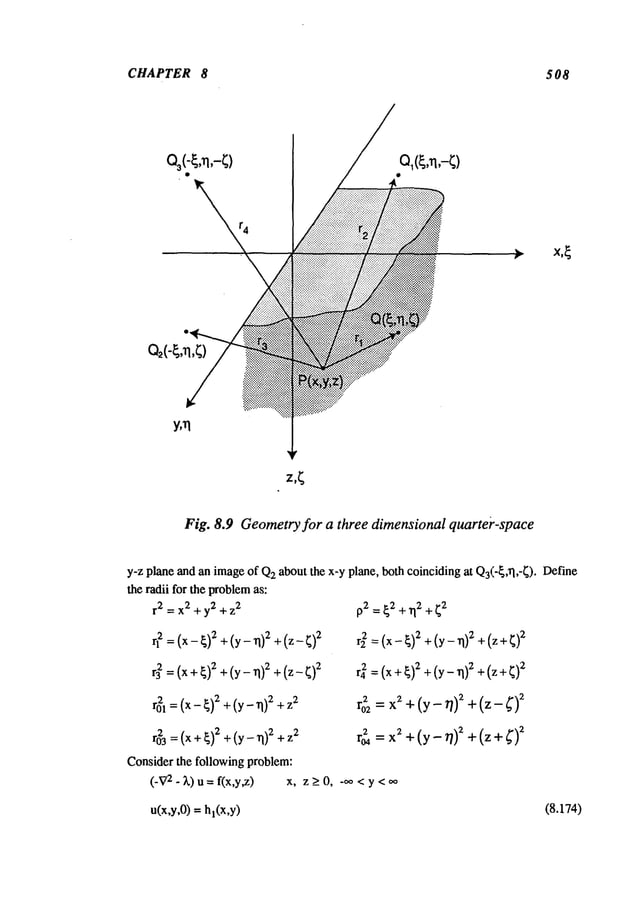
![CHAPTER 8 510
(4) Thesign is the sameas the source if the imageis reflected overan extensionof the
Neumannboundary.
Withthis construct, the sign for C
1 = 1, the sign of C
2 = -1, the sign of C
3 shouldbe the
sameas C
1 because of the reflection about a Neumann
boundaryextension and should be the
oppositeof C
2 becauseit is a reflection about the Dirichlet boundaryextension, i.e.
C3 = C1 =-C2 = +1.
8.33 Causal Green’s Function for the WaveOperator in
Bounded Media
Considerthe waveoperator:
-c2V2 u(x,t)= f(x,t) x in R, t > 0
together with the initial and boundaryconditions:
u(x,0) = fl(x) O-~.u(x,0) = x in R
(a) Dirichlet: u(x,t)ls = h(x,t) x on S
8u
(b) Neumann: ~(x,t)ls = h(x,t) x on S
3u
-ffffn(x,t)+
Vu(x,t)l
s =h(x,t)
(c) Robin: x on S
Thecausal fundamentalGreen’sfunction g(x,tl~,x) wasdefined in (8.109). Consider
adjoint causal fundamental
Green’sfunction g(~,zlx,t) whichsatisfies:
(~2- C2V
2] g(~,’~lx, t) = ~5(~- x) 6(~:-
(8.108)
g(~,’clx,t): 0 a: <
It shouldbe notedthat since the wave
operator is self-adjoint, then:
g(x,tl~,x)
=g(~,xlx,t) (8.176)
Considerthe special case of a time-independentregion Rand surface S. Substitute u(x,t)
fromabove, eq. (8.108) and the adjoint causal Green’sfunction v = g(~,xlx,t) into Green’s
identity for the waveoperator (8.52). Since the regionRand its surface S do not change
time, the surface ~ takes a cylindrical surface form shown
in Figure 8.10. Onthe
cylindrical surface S, n = n, while on the surface t = 0 and t = T, the normal
~ = -~t and ~t, respectively.](https://image.slidesharecdn.com/advancedmathematicalmethodsinscienceandengineering-hayek-230318001731-2b30ece5/85/advanced-mathematical-methods-in-science-and-engineering-hayek-pdf-517-638.jpg)
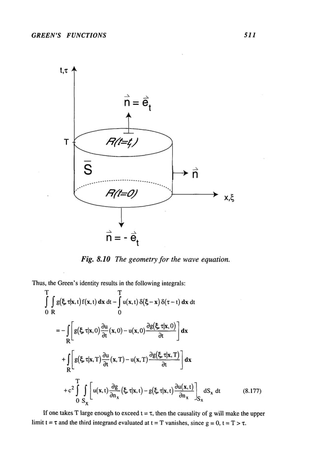
![CHAPTER 8 512
Since0gl0t = -0gl0z, then eq. (8.177) can be simplified to:
u(~’c)
=f f g(~xlx,
t)f(x,t)
OR
+
y ,x,o+
x+ o>
R R
-c2f f [u(x,t)O-~x(~Xlx, t)-g(~xlx, 1 dSxdt (8. 178)
0 S
x
sx
Onecan rewrite the last expressionby switchingx to ~ and t to x and vice versa after noting
that g({,’~lx,t)=g(x,tl{,z) giving:
t
u(x, t): ~ f g(x, tl~ z) f(~, x)d~dz +f g(x, tl~, 0)fg
OR R
t
O~_c2f Iu0g gOU] dS~dx
+~-~g(x,
ti~0)f,(~) IL
R 0 S~
Theexpressionshowsthat the responsedependslinearly on the initial conditions.
(8.179)
Example8.13 Transient vibration of an infinite string
Obtainthe transient responseof an infinite stretched string undera distributed load
q(x,t), which
is initially set in motion,suchthat:
02UC2__O2U
= q(x,t) -,~ <x <
Ot 2 0x 2 T
O
u(x,0) = fl(x) -~(x,0) =
For the one dimensionalproblem,see (8.121):
g(x,tl~, x)=H[
(t-x)-lx- ~] /c] H( t- z)
TheHeavisidefunction can be replaced by:
H(a-lbl) = H(a-b)+ H(a+b)- 1 for
Thus,the function g can be rewritten as:
g(x, tl~, x)= ~c {H[(t- x)- (x - ~)/c] + H[(t- z)+ (x -
Foran infinite string, the boundary
conditionintegrals in (8.179) vanish, leaving integrals
on the source and the twoinitial conditionsin (8.179). Thefirst integral on the source term
can be written by:](https://image.slidesharecdn.com/advancedmathematicalmethodsinscienceandengineering-hayek-230318001731-2b30ece5/85/advanced-mathematical-methods-in-science-and-engineering-hayek-pdf-519-638.jpg)
![GREEN’S FUNCTIONS 513
t
~c f q(~’ x~) H[(t-x)-I×- ~[/c] d~ dx=
%
0
Thesecondintegral can be written as:
t x + c(t-z)
1
2cTo f f q(~,z)d~
o
oo x+ct
_
1
if f f2(~)d
~
2c
--oo x - ct
Thethird integral onthe initial conditionrequires the timederivative of g:
~g {x,t~t ~ ~’ 0+)= ~c {~[t-(x-~)/c] + ~[t+ (x-~)/c]}
so that the third integral becomes:
OO
=1 j" f~(~){~[t_(x_~)/c]+~[t+(x_~)/c]}d~=~[fl(x+ct)+f~(x_ct)
]
2c
Thefinal solution for u(x,t) becomes:
t x +c(t--z) x +ct
1
u(x,t)=
f2c ~ q(~’X) d~dx +½[fl(x+ct)+fl(x-ct)]+-~-cT
O ~ f2(~)d~
0 x - c(t-x) x - ct
For a boundedmedium,
the requirement to specify u and Ou/~non the surface makesthe
problemoverspecified and the solution non-unique.Let the auxiliary causal function ~ to
satisfy:
~2~ C2X72~ = 0 x in R, t > 0 (8.180)
Ot
2
5=0 t<’~
Followingthe development
of (8.179) for g, one obtains:
t
O=f f ~(x,t[~,~)f(~,x) d~ dx + f ~(x,t[~,O)~-t (~,0) ~
OR R
- _ ~u
dz
f tl ,0) c2f f u - g ~n---~
R 0 S~
Subtractionof the twoequations(8.179) and (8.181), together with the definition
G=g - ~, results in the final solution:
t
u(x, t)= f f G(x, t]~ "Qf(~ z)d~ d~ +~ G(x, t[~, 0)f2(~) ~
0R R
(8.181)](https://image.slidesharecdn.com/advancedmathematicalmethodsinscienceandengineering-hayek-230318001731-2b30ece5/85/advanced-mathematical-methods-in-science-and-engineering-hayek-pdf-520-638.jpg)
![CHAPTER 8 514
t
G v-| dS~dz (8.182)
+-~fG(x’tll~O)fl(~)dl~-C2fs~IUOn3---~G~-
R 0 0n~ JS~
For the following boundaryconditions, one must set conditions on the function Gas:
(a) Dirichlet: G[S
~ = 0
(b) Neumann: 3a- ~- = 0
S~
3G ~YGs~ =0
(c) Robin:
3n~
Theboundaryintegrals in (8.18) take the formsin eqs (8.132 - 8.135).
Example8.14 Transient longitudinal vibration in an semi-infinite bar
Obtainthe transient displacement
field of a semi-inifinite bar at rest, whichis set in
motionby displacing the bar at the boundaryx = 0. Thesystemsatisfies the following
equation:
32u 32u
= 0 u(x,O) = -~(x,O) = u(O,t)= h(t)
2
3t 2 c 3x
~
Usingthe method
of images,let the imageof the source at ~ be located at --~, giving:
1
x
G=2--
~-
TheGreen’s function satisfies Gx = 0 = 0 if C = 1. RewritingG in a moreconvenient
form using:
H(a-lbl) = H(a-b) + H(a+b)- 1 for
1 {H[(t-x)-(x-~)/c]+H[(t-x)+(x-~)/c]
G=2--
~
-H[(t- ~)- (x + ~)/c]- H[(t- x) + (x + ~)/c]}
30
= - 6[t - "c - x/c]
3n¢~=0 ~’~=0
givingthe final solution:
t
~ h(’c) 6[t - x - x/c] dz = h(t - x/c) H(ct
t)
0](https://image.slidesharecdn.com/advancedmathematicalmethodsinscienceandengineering-hayek-230318001731-2b30ece5/85/advanced-mathematical-methods-in-science-and-engineering-hayek-pdf-521-638.jpg)
![CHAPTER 8 51 6
T
~U _u ~g
]
J"[g* c~n:~
_Is,
dSxdt
0 S
x
- ~ u(x,0)g’(x,01~,x) dx + ~ u(x,T)g’(x,’l~,x)dx
R R
Again
sinceg*is causal, let Tb~takenlargeenough
so that g = 0 for t = T> x.
Rea~.’ranging
thetermsgives:
OR
* - u~ dSx dt (8.185)
R 0 S x ~ Snx s,
Fora bounded
meAium
let the auxiliary causalfunction~ satisfy:
=o
~t
~ =0
andthe adjointcausalauxiliaryfunction~*satisfies:
- ~t* - ~:V2g*
= 0
g =0
Using
~(~, xlx, t) = ~*(x,~, x) into theGreen’s
identity(8.48)resul~sin anequation
similarto (8.185):
O=j"
~~*(x, tl~,x) f(x, t) dx
OR
+fu(x,0)~’(x,0[~,x)dx+gf[~" 8u_~. ~u? dSxdt (8.186)
R Sx ~nx
Onx
Subh-action
of (8.186)from(8.185)andusingthe definitionG*= g*- g[*results
OR](https://image.slidesharecdn.com/advancedmathematicalmethodsinscienceandengineering-hayek-230318001731-2b30ece5/85/advanced-mathematical-methods-in-science-and-engineering-hayek-pdf-523-638.jpg)
![GREEN’S FUNCTIONS 517
R 0 Sx 0n--~-- u On---~-jsxdSxdt
Switchingx to ~ and t to x andvice versa andrecalling ~at:
G*(~xlx,t) = G(x, tl~x)
one canrewrite the last expressionto:
t
u(x, t)= f f G(x, tl~z)f(~ ~)d~
0R
t[
+ffl(~)G(x, tl~O)d~+~:j" J" G °~u uol
R 0S~ 3--~-~ - 3n~ JS~
whereG= g - ~. Thus,for the different types of boundaryconditions:
(8.187)
(a) Dirichlet: GIs
t = 0
(b) Neumann: ~a-~-- = 0
s~
~G St
(c) Robin:
~n-~ + ?G = 0
Theboundaryintegrals follow the sameforms as in eqs (8.132 - 8.135).
Example 8.15 Heat Flowin a Semi-Infinite Bar
Considera source-freesemi-infinite bar being heatedat it’s boundary,
such that:
OU-KV2u= 0 x > O, t > 0
Ot
u(x, +) =0 u(0,t) =o h(t)
Toconstruct G(x,tl~,’r) for a Dirichlet boundarycondition, then both conditionsmust
satisifed; G(0,tl~,x)=0 andG(x,tl0,x)
ThefundamentalGreen’sfunction g(x,tl~,x) is given in eq. (8.106). Toconstruct
auxiliary function ~, let the imagesourcebe located at (-~) suchthat:
-(x+~)
2/[4~:(t-z)]
~(x,t I -~, z) =C H(t- "~)
[4n~:(t- "c)]
then to makeG(0,tl~,x)
= 0 requires that C= -1, and G becomes:](https://image.slidesharecdn.com/advancedmathematicalmethodsinscienceandengineering-hayek-230318001731-2b30ece5/85/advanced-mathematical-methods-in-science-and-engineering-hayek-pdf-524-638.jpg)
![CHAPTER 8 518
H(t
- "~)
{e-(X-~)
~/[4~c(t-~:)]
_ e-(X+~)~/[4~c(t-~:)]
}
G-
11/2
Thefinal solution requires the evaluation of 0G/0n~:
(gG
=
_ 0G x H(t - x)
e-X
2/[4~:(t-’t:)]
~--on~= 0 ~ ~ = 0 4~-[K(t ,~)]3/2
Therefore, the temperature distribution in ~e bar due to the non-homogeneous
bound~y
condition is given by:
t
UoX f h(z)
~J 0 (t _ x)3/2 e-X:/[4~(t-x)]
D(x,t)
=
Example 8.16 Temperature
distribution in a semi-infinite bar
Findthe temperaturedistribution in a source-free, semi-infinite solid bar with
Newton’s
law of cooling at the boundarywherethe external ambienttemperatureis uoh(t),
suchthat the temperature
u(x,t) satisfies:
oqu o32u
---K =0 x>0, t>0
0t ~ -
oqu
u(x,0) =
0x
--- (0, t) +y u(0, t) =o h(t
Herethe boundarycondition is the Robincondition such that:
or
~--~ + y G OG
--~x +yG =0
x=0
Let the function w(x,t]~,x) be definedby:
OG
w(x,tl~,x) = -~x Y G
Substituting winto the diffusion equation and recalling that G= g - 5, then:
~t ~x2) :(’~’x-’-~--~c~-~-~I-L-~x-’)L--~--
~’~-~’}
L~x -~)-y6(x-~) 6(t-~)](https://image.slidesharecdn.com/advancedmathematicalmethodsinscienceandengineering-hayek-230318001731-2b30ece5/85/advanced-mathematical-methods-in-science-and-engineering-hayek-pdf-525-638.jpg)
![GREEN’S FUNCTIONS 519
together with the boundarycondition on w, w(0,t[~,x) = 0. This showsthat the function
wsatisfies the Dirichlet boundarywith the aboveprescribed source term. TheGreen’s
function for a Dirichlet boundarycondition is given in Example
(8.15):
w(x,tl~,x)
=f f G(x,t[ n,~)I0~-(n-
~)-‘/~(n-~)1~(~-
00
H(t - x)
~/4~tK(t- ~)
{y[e-(x+~)~/[4~(t-’r)] e-(X-~)
~/[4~(t-’l:)]]
Integrating the equationfor G, oneobtains:
G = -e~x f w(u,t I ~,x)e-~u du
X
Integrating byparts the secondbracketedquantity in w, results in the following
expressionfor G:
H(t-’c) [e-(X-~)2/[4~(t-,r)] _ e-(X+~)
z/ [4~(t-z)]]
G(x,t
I ~,~)
[! e-~ue-(u+ 1
H(
- 2‘/e
Yx {)~/[4K(t-x)]du
Thelast expressionin the integral formcan be shown
to result in:
-~ H(t - ~)et[x+{+~/(t-x)l erfc ’~-(t
Note that if,/= 0, one retrieves the Green’sfunction for Neumann
boundarycondition. If
the limit is takenas ’/--) oo, then one obtains the Green’sfunction for Dirichlet boundary
condition, matchingthat given in Example
(8.15).
Thefinal solution is given by:
t
u(x,t) K:y Uo
j-G(x,t I 0,x)h(x)dz
0
8.35 Methodof Summation
of Series Solutions in Two-
Dimensional Media
TheGreen’sfunction can also be obtained for twodimensionalmediafor Poisson’s
and Helmholtzeqs. in closed form by summing
the series solutions. This methodwas
developedby Melnikov.Since the fundamentalGreen’sfunction is logarithmic, then all](https://image.slidesharecdn.com/advancedmathematicalmethodsinscienceandengineering-hayek-230318001731-2b30ece5/85/advanced-mathematical-methods-in-science-and-engineering-hayek-pdf-526-638.jpg)
![CHAPTER 8 520
the Green’sfunctions will involve logarithmic solutions as well. This methoddepends
on the following expansionfor a logarithmic function:
log~/1- 2ucos~+ u2 = - ~ ---if- cos (n~) (8.188)
n=l
providedthat lul< 1, and 0 < ~ < 2n
Themethodof finding the Green’sfunction dependson the geometryof the problemand
the boundaryconditions.
8.35.1 Laplace’s Equation in Cartesian Coordinates
In order to showhowthis methodmaybe applied it is best to workout an example.
Example 8.17 Green’sFunctionfor a Semi-Infinite Strip
Considerthe semi-infinite strip 0 < x < L, y >0 for the function u(x,y) satisfying:
-V2u= f(x, y) < x < L,y >0
Subjectto the Dirichlet boundary
conditiononall three sides, i.e.:
u(0,y) = u(h,y) = u(x,0) =
and u(x,~) is bounded.
Onemay
obtain the solution in an infinite series of eigenfunctionsin the x-
coordinates, since the two boundaryconditions on x = 0, L are homogeneous.
These
eigenfunctions are given by sin (nnx/L) [see Chapter6, problem2], whichsatisfies the
two homogeneous
boundary conditions.
Let the final solution be expanded
in these eigenfunctionsas:
OO
u= ~ Un(Y)sin(~x)
n=l
Substituting into Laplace’sequation and using the orthogonality of the eigenfunctions
one obtains:
n2~z
2
d2un (._~_) Un = _ fn(y
)
dy
2
where
n=1,2,3 ....
L
fn(y) = ~ j" f(x, y)sin (-~
0
Thesolution for the non-homogeneous
differential equation is given by the solution to
Chapter 1, problem7d:
Y
Un(Y)= n sinh ( ~-y)+ B
n cosh (-~-y)+ ~j"fn (~])sinh (-~ (y- rl)) q
0](https://image.slidesharecdn.com/advancedmathematicalmethodsinscienceandengineering-hayek-230318001731-2b30ece5/85/advanced-mathematical-methods-in-science-and-engineering-hayek-pdf-527-638.jpg)
![GREEN’S FUNCTIONS 521
Since u(0,x) = 0, then n =0 and:
Y
nn L I fn (.q) sinh (~ (y _ ~l))
Un(y
) =A
n sinh(-~-- y) +~--~-~
0
Alsosince u(x,~o)is bounded
then:
An= - ~-~ I fn (~l) e-nml/L
l
0
Thefinal solution is then:
Un(Y)
= ~ I fn (~1)[enr~(Y-’O)/LH(II
- Y)
- e-nr~(y+rl)/L + e-nr~(Y-rl)/LH(~l
- y)] d~l
0
Thus,the Green’sfunction for the y-component
is given by:
L [e-nn(y+~l)/L - enn(y-~l)/L Y<~l
Gn
(Y[ ~1)=2--~-~[e-n~(y+~l)/L~
e
-nr~(y-rl)/L y>rl
Notethat Gn(01~l)
=
Thus,the solution for Un(Y)
is given by:
Un(Y)
= f Gn(yI rl)fn(rl)d~l = -~ I f Gn(Y
I rl) f(~’rl)sin ~)d~d~l
0 00
oo Loo
u(x,y)= ~ E f I Gn(YI ~l)sin(~ ~) sin(~x)f(~,’q)d~d~l
n=100
= I It-~ E Gn(Ylrl)sin(~)sin(~ x) f(~,rl)d~drl
00L n=l
Thus,the Green’sfunction G(x,yl~,rl) is given by:
G(x, yl~,n)=~ Gn(Y
n=l
n) sin (-~--~)sin (-~-
L L
L Gn(Y
n=l
For the region y >](https://image.slidesharecdn.com/advancedmathematicalmethodsinscienceandengineering-hayek-230318001731-2b30ece5/85/advanced-mathematical-methods-in-science-and-engineering-hayek-pdf-528-638.jpg)
![CHAPTER 8 522
1 1 exp(-
(y+’q))-exp(---L-(Y-~l))¯
G(x,y I {, ~1) :
n
n=l
Usingthe summation
formula(8.188), on the first of four terms, one gets the following
closed form:
1
~ E exp(---~--(y
Here:
n=l
+~1))
cos(~(x-
u= exp(-~(y + rl)) ¢~ = ~(x- ~)
= ~--~1 log./1-2exp(-~(y+ rl))cos(~(x-~))+ exp(---~(y
z~ V L
Similarly, one obtains the closed formfor each of the remainingthree series, resulting in
the final form:
1 AB
G(x,y ] ~, ~1)= ~ log (~--~) (8.189)
where:
A=I-2exp(~(y+ ~l))cos (~ (x - ~)) + exp (-~(y
2r~
B=1 - 2 exp(~ (y - rl)) cos(~ (x +~)) +exp( _--7-(Y
L L L
C= 1-2 exp(~(y-n))cos (~(x- ~))+ exp(-~
D=i-2exp(~(y + rl))cos (~(x q-~))+ exp(-~ (y
Themethodof images wouldhaveresulted in an infinite numberof images.
8.35.2 Laplaee’s Equation in Polar Coordinates
Theuse of the summation
for obtaining closed form solutions for circular regions in
twodimensionscan be best illustrated by examples.
Example 8.18 Green’sFunctionfor the lnterior/Exterior of a Circular Regionwith
Dirichlet BoundaryConditions
First, considerthe solution in the interior circular regionr <a withDirichlet
boundarycondition governedby Poisson’s equation, such that:
--g72U = f(r,0) u (a, 0) = 0 < a,0 <0 < 2rt](https://image.slidesharecdn.com/advancedmathematicalmethodsinscienceandengineering-hayek-230318001731-2b30ece5/85/advanced-mathematical-methods-in-science-and-engineering-hayek-pdf-529-638.jpg)
![CHAPTER 8 524
- log(O_) r _<
p
Go(rI p) a
- log(L) r>_
p
a
It should
benotedthat Go(alp)
= Go(rid)= 0 as requiredbythe Dirichletbmmdary
condition.
c,s (r) resultsin thefollowing
solution:
Integrating
the differentialequation
for un
u~,S(r)-¢.s -n _
n 2.oLLr;
f.’(p)pdp
C,$
Again
un (0) is bounded
requires
that n =
0 an
d th
e bo
undary on
r =a requ
ires that
:
2ha
n
- f~"(p)pdp
Thus,
thefinal solution
for u~
’s (r) becomes:
i r n 1. n | rna n a
n
fC(P~-(--~ l’~’S(p)pdp-~n/;)I I-~)-l~)3
f~’s(p)
which
canbewritten as:
1 (r~
na’r’p’n
a
= ~O,(r
Ip)fnC"(p)pdp
0
where
---1[lr~n- (-rP~n for r_<
2nLLp) La29 J
P
Gn(rI p)
1---If O-~
n (rP’~n] for r>p
2nL
r -La
--e)
J
Note
that
Gn(alp)
=Gn(rla)
=0asrequired
by
the
Dirichlet
boundary
condition.
Finally,
the
solution
for
u(r,O)
is
obtained
bysolutions
into
the
original
eigenfunction
expansion:](https://image.slidesharecdn.com/advancedmathematicalmethodsinscienceandengineering-hayek-230318001731-2b30ece5/85/advanced-mathematical-methods-in-science-and-engineering-hayek-pdf-531-638.jpg)
![GREEN’S FUNCTIONS 525
a
u(r,0) JG
o(r I 0)fo(P)PdP
0
oo a
+ £ IGn(rlP)[f~(o)c°s(nO)+fSn(O)sin(nO)]pdo
n=10
2n a
:._~_1 I I G°(r]o) f(p,*)pdpd*
2n
O0
~ 2~ a
1
+-- E I I
Gn(r [o )[ c°s(n~)c°s(nO)+sin(n*)sin(nO)lf(p’*)odpd*
n=lo0
1 ~ ~Go(rl0) f(0,~)pdpd
~
2~
00
~ 2g a
1 IG~(
r
+; 2 I
IP)C°s(n(O-~))f(o’*)pdpd*
n=l 0 0
Thus, the Green’s function becomes:
a(r,019,0) = ao(rl9)+2 Gn(r I O)cos(n(0-
n=l
Theseries can be summed,
eq. (8.188) as:
2£ Gn(rlp)cOs(n(0 (p)) £ 1 /~)n
.... cos (n(0- tp))
n
n=l n=l
=½log
1 - 2 (~-~) c°s (0 - q°) + (~-~)2
1 - 2 (r) cos(0
P P
." ( 1 - 2 (~) cos (0 - + (~)
2 (1_2(~)COS(0 ~)
where~ = a2 / p is the location of the imageof the source at p. Therefore:
G(r’01 ~’~) = ~ {-l°g(~)~ +l°g[( ~ - 2r’c°s(~-~)+r~
=~log(P2
the notationfor r2 and r~ are givenin section (8.28). Notethat the last answeris the
sameas the one given in (8.142).
(8.190)](https://image.slidesharecdn.com/advancedmathematicalmethodsinscienceandengineering-hayek-230318001731-2b30ece5/85/advanced-mathematical-methods-in-science-and-engineering-hayek-pdf-532-638.jpg)
![GREEN’S FUNCTIONS 52 7
Finally, the function u~
’s (r) canbe written in compact
formas:
G
n (r I P) = 2n L P) ~, a2 )
lI(19~n +( rlg"]n
1
2nL
rJ t, a2) j
for r>p
¢,S
Substituting Go(rip) and Gn(r[p)into the solutions for n and those in t urn into t he
seres for u(r,0) results in the solution givenby:
2n a " ~
1 ~ ~ Go(r~p)+2E Gn(rlP)COS(n(0-~)
)~ f( p, ~)pdpd#
00 n=l
Summing
the series results in the formgiven in (8.188):
G(r,0 ’ P,*) : ~ { ’og(~)~ - log(’- 2(~) cos (0- O)
{ }
1 log
+ logp2~2_ log ( )
4g
I, (r~r~
Thelast expressionis written in the notation of section (8.28) andmatchesthe solution
given in eq. (8.144).
TheGreen’sfunction is symmetric
in (r,p) and satisfies:
(a,01P,*) = ~(r,01 a,0)
In the exterior region, one mayuse the fo~ in eq. (8.191) with the notation at the
source p > a and its image~ = a~ / p < a.
where:
a
u~,S(r) = IGn(r I p) f~’s(p)pdP
0](https://image.slidesharecdn.com/advancedmathematicalmethodsinscienceandengineering-hayek-230318001731-2b30ece5/85/advanced-mathematical-methods-in-science-and-engineering-hayek-pdf-534-638.jpg)
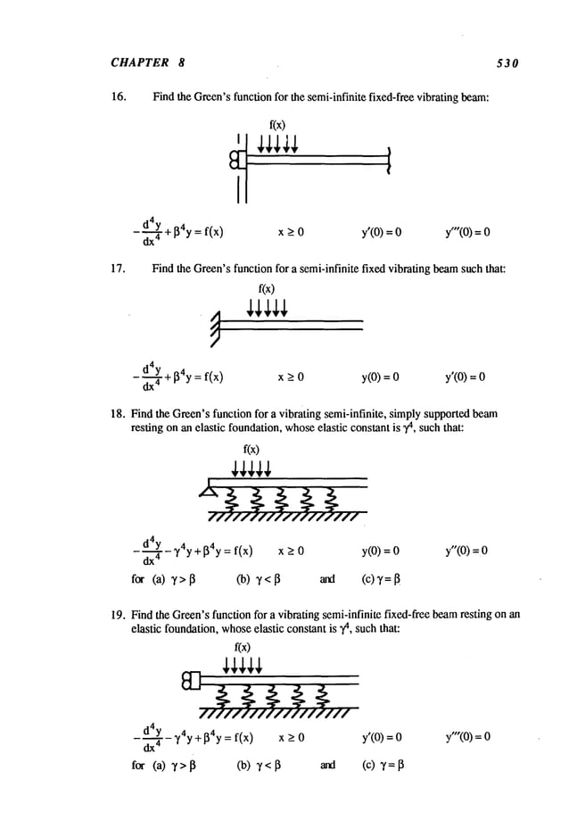
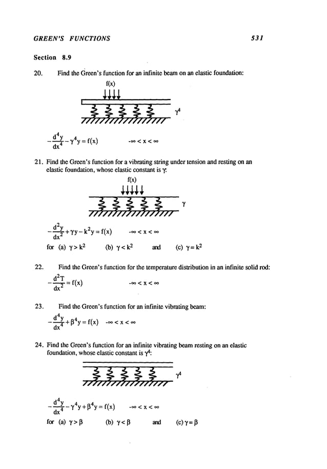
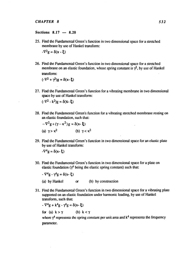
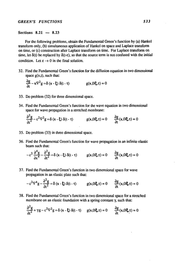
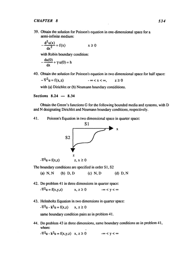
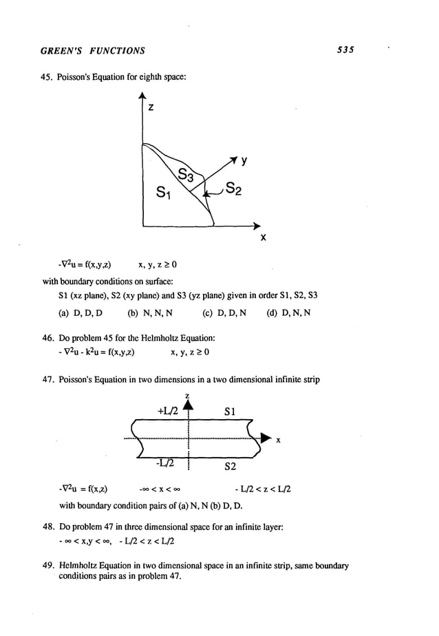
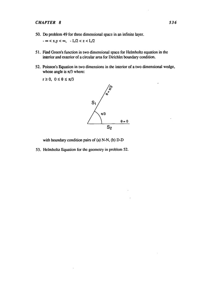
![ASYMPTOTIC METHODS 541
=f(’)(zo)
an
n!
Due to the definition of the SPat z0, then the secondtermvanishes, since:
a1 =f’(zo) =0
If, in addition, a2(z
o) = a3(zo)..... am(Z0)
= 0 also, so that the first non-vanishing
coefficient is am+
l, then, in the neighborhood
of zo, f(z) canbe approximated
by the first
twonon-vanishingtermsof the Taylorseries aboutzo, i.e.:
f(z)= f(z0)+(z-z0) m+l fCm+l)(z0)
(m
whereterms of degree higher than (m+l) were neglected in comparisonwith the (m+l)
st
term. Defining:
f(m+l)(zo) = ae
ib
(m+ 1)!
and the local topographynear the SPzo by:
Z- Z0 = r ~i0
then the function f(z) in the neighborhood
of the SPcan be describedby:
f(z) = f(z0) + aeib(rei°)m+l= u0 + iv0 +rm+lae
i[(m+l)O+b]
where:
u0 = U(Xo,Y0) v0 =v(x0,Y
0)
Hence,the real and imaginaryparts of f(z) in the neighborhood
of o are, r espectively:
u = uo + arm+lcos[(m+l)0+b]
v = vo + arm÷lsin[(m+l)0+b]
Thesteepest descent andsteepest ascent paths are given byv = vo = constant, or:
sin[(m+l)0+b] =
Thevarious paths of steepest ascent or descent havelocal orientation angles0 with the
x-axis given by:
n~ b
0= n=0,1,2 ..... (2re+l)
m+l m+l
Substitution of 0 in the expressionfor u(0) aboveandnoting that, for steepest descent
paths, uo has a local maximum
at zo on C’ and hence, u - uo < 0 for any point (x,y)
C’, then cos(m0< 0, indicating that n must be odd. Thenumberof steepest descent paths
are thus (m+ 1), and are definedby:
2n+l b
0SD P = ~x-~ n =0, 1, 2 ..... m
m+l m+l](https://image.slidesharecdn.com/advancedmathematicalmethodsinscienceandengineering-hayek-230318001731-2b30ece5/85/advanced-mathematical-methods-in-science-and-engineering-hayek-pdf-548-638.jpg)
![CHAPTER 9 542
Fig. 9.1
Toevaluatethe integral overCin (9.4), the original pathCmustbeclosedwithany
twoof the 2mSDP
paths C’, call themC~andC~,eachoriginating fromzo. Invoking
the Cauchy
Residuetheoremfor the closed path C + C~+ C~let:
w= f(z0)- f(z) o + iv
o)- (u +iv)
Thepreceding
equalitycan beusedto obtaina conformal
transformation
w= w(z),
eachof the twopaths C~andC~whichcanbeinverted to give z = z(w). "[his
transformation
fromthe z-planeto the w-plane
transforms
the original pathCas wellas
the pathsC~,
2 to new
pathsin the w-plane.It shouldbenotedthat this conformal
transformation
is usuallynot easily invertable.
Sincev = vo onC~,
2, thenthe functionwis real onthe twoSDP
C~,
2, i.e.:
wlc~,c~
=Uo-
u
When
z = z0, thenw= 0 andwhen
Izl onC~,
2 --> 0%
w---> oo,so that the integralson
C~,2are
performed
overthereal axisof thew-plane,
i.e.:
IC~2=
fe°If(zo)-w]~(w)[~ww]dw=e
pf(z°)fe-0w ~(w) dw (9.10)
¯ (dw
/ az)
0 0
where
~(w)= F(z(w))and(dw/dz)are complex
functionin the w-plane,since
conformal
transformation
z -- z(w)is complex.
~(w)
Expanding
(dw/dz"~’~
in a Taylorseries in waboutw= O,then:
~(w)
= Z ~n wn+V
(9.11)
(dw/dz)
n=0](https://image.slidesharecdn.com/advancedmathematicalmethodsinscienceandengineering-hayek-230318001731-2b30ece5/85/advanced-mathematical-methods-in-science-and-engineering-hayek-pdf-549-638.jpg)
![ASYMPTOTIC METHODS 543
wherev is a non-integerconstant, resulting fromthe derivative dw/dz.
It shouldbe noted that the slope dw/dzhas a different value on C~and C[.
Substituting eq. (9.11) into eq. (9. I0), integrating the resulting series termby term,
using Watson’sLemma
in (9.3), the integral in (9.10) becomes:
Ic[2 ~ ePf(z°) Z ~n F(n + v + 1)
9n+v+l
(9.12)
n=0
Notethat Ic~ and Ic~ havedifferent series basedon the path taken. Thus,if Cis an
infinite path, and one mustclose it with an infinite path, then twopaths C[2mustbe
joined to C, resulting in:
IC = Ic~ - Ic~ + 2hi [sumof residues of the poles between C+C~+C~] (9.13)
Thesign for the residues dependson the sense of the path(s) of closure betweenC, C~,
and C~, whichmaybe clockwise for somepoles and counterclockwisefor other poles.
Thepaths C~and C~start fromw = 0 and end in w= ~ along each path, so that the sign
assigned for C~is negative.
9.5 Debye’s First Order Approximation
Thereare first order approximations
to the integrals in eq. (9.10). Principally, these
approximationsassumethat the major contribution to the integral comesfromthe section
of the path near the saddle point, especially when13 is very large. This means
that the
first termin eq. (9.12) would
suffice if 13is sufficiently large. Toobtainthe first order
approximation,one can neglect higher order terms in ~(w) and (dw/dz) in such a way
a closed formexpressioncan be obtained for the first order term. Thus,an approximate
value for w can be obtained by neglecting higher order terms in w:
w=f(z0)- f(z) =-(z- m+l f(m+l)(zo)
(m+ 1)!
(9.14)
Thus,for z near z0, the conformaltransformation betweenw and z can be obtained
explicitly in a closed form by the approximation:
1/(m+l)
(m+1)!
w
1/(re+l) = Jew]
1/(re+l) (9.15)
(z-z0) = f(m+l)(zo
)
wherethe complexconstant c is given by:
(m+l)!
C= f(m+l)(z0)
Notethat the (re+l) roots havedifferent values alongthe different paths C~n.
Differentiating this approximation
for z withrespect to wresults in:
dz cl/(m+l)w
-m/(rn+l)
dw m +1](https://image.slidesharecdn.com/advancedmathematicalmethodsinscienceandengineering-hayek-230318001731-2b30ece5/85/advanced-mathematical-methods-in-science-and-engineering-hayek-pdf-550-638.jpg)
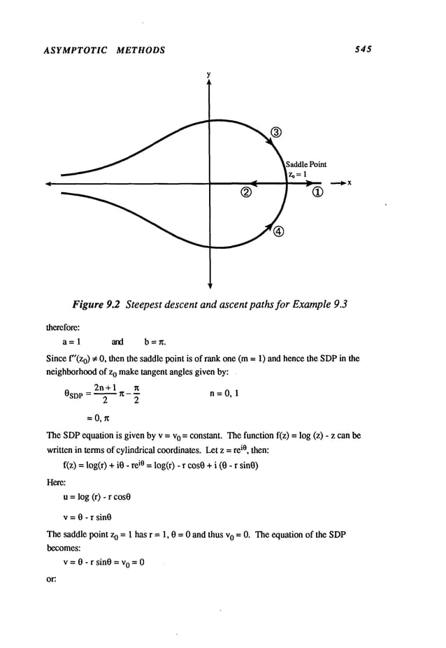
![CHAPTER 9 546
0
sin 0
Thefour paths are shownin Figure 9.2.
It can be seen that in the neighborhood
of the saddle point zo = 1, the pa~ts 0SD
P = 0,
x are paths "1" and "2", so that paths "3" and "4" are the steepest ascent paths.. Path"2"
extendsfromz = 1 to 0 and path "1" extendsfrom1 to oo. It turns out that the original
path on the positive real axis represents the twoSDP’s,so that there is no needto deform
the original path into the SDP’s.Theleading term of the asymptoticseries for the
Gamma
function can be written as (9.18):
F(k+ 1) = k+l e-k~/-~ = e-k kk+I/2
IK
Example 9.4
Find the first order approximation
for Airy’sfunction definedas:
Ai(z>: cos(s3/a+sz)ds = ~ exp i(s3/a+sz ds
0
Toobtain an asymptoticapproximation
for large z, the first exponential terms is also not
a slowly varying function. Tomergethe first exponential with the second, let s = ~ t:
Ai(z) "~- ~exp[iz3/2(t3/3 + t) ] dt
Letting x = z3/2 onecan write out the integral as:
_ 1/3 oo
Ai(x2/3) = -~-~ ~ exp[ix(t3/3 + t)]
Onecan evaluate the first order approximation
for large x. In this integral F(t) = 1 and
f(t) -- i (t3/3+
Thesaddlepoints are givenby f’(t o) = i (to2 +1) = 0 resulting in twosaddlepoints,
to = +i. To mapthe SDP:
f(+i) -2
3
f"(+i) =-T-2
Hereb = 2 and 0 = ~ for to = +i and0 = 0 for to --- -i. It shouldbe notedthat since
g’(to) ~ 0, m= 1 for bothsaddle points. Letting t = ~ + i~l, then the SDP
path equations
for both saddle poinls are given by:
v(~,rl) = Im f(t) = ~3/3- ~1 + ~ : v0(~0,~10)= v0(0,+l) :](https://image.slidesharecdn.com/advancedmathematicalmethodsinscienceandengineering-hayek-230318001731-2b30ece5/85/advanced-mathematical-methods-in-science-and-engineering-hayek-pdf-553-638.jpg)
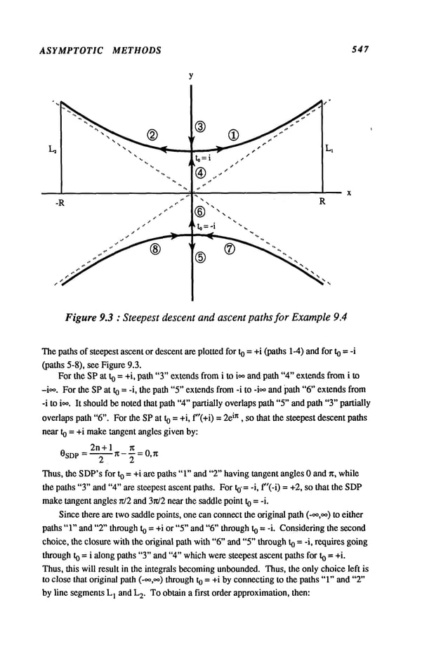
![CHAPTER 9 548
xl/3 1.
~f
-1/6
=--. eX(_2/3) 2r~ _ x_ __ e_2X/3
Ai(x)
-(--~x) 4~/~
sothat:
Ai(z)=
z-’/4 ( 2/3]-~--~
exp
--~
9.6 Asymptotic Series Approximation
Tofind an asymptoticseries approximationfor an m
th ranked SP, one can return to
the Taylorseries expansionfor the functions within the integrand in (9.10).
approximationto the asymptoticseries (9.10) can be obtained using an approximationfor
the derivative dz/dw.Letting:
w = f(zo)- f(z
)
_ (z-Zo) m+l I1 + (z-z°)f(z0)(m+2)
cL m+2 f(z0)(m+l)
(z- Zo)2 f(Zo)(m+3) 1
(m+2)(m+3)f(zo)(re+l)
then:
dW_dz
(m+l)c
(z-z0)m
I1+(z- Z°)m
f(z0
)(m+2)f{z0~(
m+l
)~, )
(9.19)
(Z-Zo) 2 f(zo) (m+3) ]
+ (m+l)(m+2)f(zo)(m+l)
(9.20)
In the neighborhood
of z = z0, then, usingthe expressionfor z - z0 in eq. (9.15), one obtains:
dw m + 1 m/(m+l) wl/(rn+l) w2/(m+l)
d’-’~- = ~
w [bo +bl +b
2 +...]
oo
(m+l) .m/(m+l)
= ~ w
Z bnwn/(m+l)
n=O
where:
bo= 1
C
(m+2)/(m+l) f(zo)(m+2)
bl =-(m+l)(m+l)!
b
2
=-
b3 =
c(m+3)/(m+l)
(m+ 1)(m+ 2)(m+ 1)! f(z°)(m+3)
C
(m+4)/(m+l)
f(z0)(m+4)
(m+ 1)(m+ 2)(m+ 3)(m](https://image.slidesharecdn.com/advancedmathematicalmethodsinscienceandengineering-hayek-230318001731-2b30ece5/85/advanced-mathematical-methods-in-science-and-engineering-hayek-pdf-555-638.jpg)
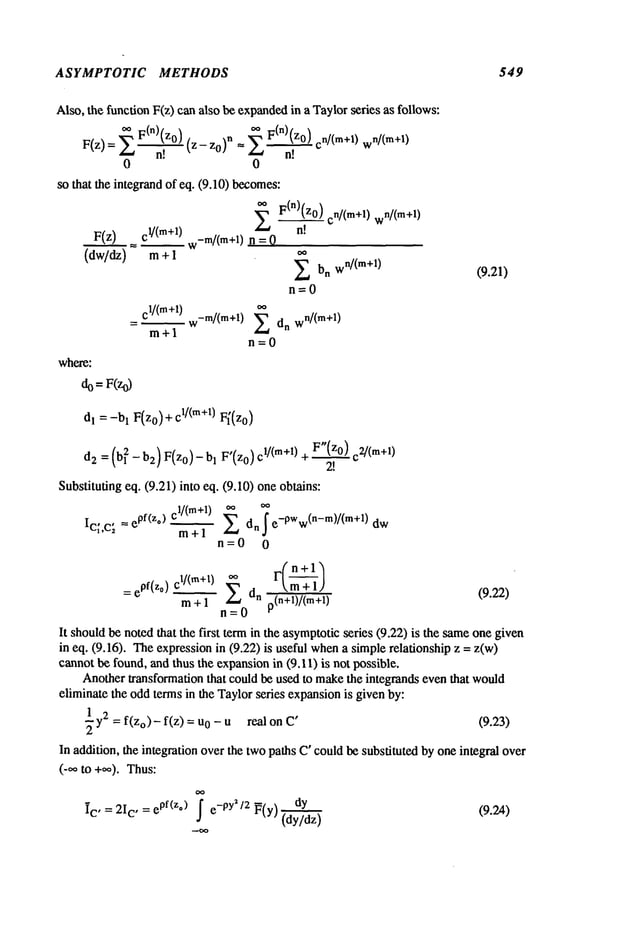
![CHAPTER 9 550
Expanding
the integrandin a Taylorseries, andretainingonlythe eventermssincethe
oddtermswill vanishgives:
~(Y) = ~ ~2n y2n+2v (9.25)
(dy/dz) n=0
where
v is a non-integer
constant.
Thus,the integralovertheentire lengthof thesteepestdescentpath(2~
c,) Can
beobtainedas follows:
~C’----2Ic ’--epf(zO) ~ ~2n S e-PY’/2 y2n+2vdy
n=O -oo
: epf(z°) S’ F(2n + 2v+_l) (9.26)
Example 9.5
Obtainthe asymptotic
series for Airy’sfunctionof Example
9.3. Starting withthe
integral givenin Example
9.3 thenthe transformation
aboutthe saddlepointat t0=+iis
givenby:
w=f(to) - f(t) =-2/3- i (t3/3+t) =(t - 02- i (t
Thepreceding
conformal
transformation
between
t andwcanbeinvertedexactly, sincethe
formula
is a cubicequation.However,
this would
result in a complicated
transformation
t = t(w). Instead,onecantry to finda good
approximation
validnearthe SPat o -- i.
Toobtaina transformation
fromt to w,wecan obtain, approximately,
an inverse
formula.Letthe term(t- i) berepresented
by:
t-i=
[1- i(t- i)/3]
1/2
Again,sincethe integral hasthe greatestcontributionnearthe saddlepoint, thenonemay
approximate
the term(t - i) by:
t-i-- +-J-~
Substitutingthis approximation
for (t - i) in the denominator
of the formula
above,one
canobtainthe approximate
conformal
transformationfromt to w:
t- i ~- 1/2
The+]- signsrepresentthe transformation
formula
for thepaths"1"and"2’" of Figure
9.3. Expanding
the denominator
in aninfinite series aboutw-- 0, oneobtains:
~,(_.+1)"
t- i
n=l](https://image.slidesharecdn.com/advancedmathematicalmethodsinscienceandengineering-hayek-230318001731-2b30ece5/85/advanced-mathematical-methods-in-science-and-engineering-hayek-pdf-557-638.jpg)
![ASYMPTOTIC METHODS 551
Thederivatives dt/dwcan be obtained readily:
dt =. 3 2 (+l)nin-1 F(3n/2-1)
w
n/2-1
aw 2 (n- 1)! r(n/2) n
n=l
Theproductof F(w)= 1 and dt/dwcan be substituted in the integral (9.10). Theintegrals
require the evaluationof the following:
r(n/2)
~
e-XWw"/2-l
aw= xn-
~
0
Thus,the twointegrals on paths "1" and "2" are given by:
3xl/3
o. (+1)" r(3n/2-1)
e-2X/3
~ ~"~_-1)!3 n xn/2
~c~,c~
=4-’-~
n=l
x_l/6
o~ (+l)n+1 in r[(3n
+1)/2]
= ~ e-2X/3 E
4n n! (9x)
n/2
n=0
Therefore:
at 3 o. (__.1)"i"-1F(3n/2-1)
wn/2-!
d-~" = 7 E (n _ ~’) ~’ff
Theproduct ofF(w)= 1 and dt/dwcan be substituted in the integral (9.10). Theintegrals
require the evaluationof the following:
_v(n/2)
~
e-XWw
n/2-1 dw - xn-~2-
/
0
Thus,the twointegrals on paths "1" and "2" are given by:
3x
~/3e_2~/3
~. (+1)
n F(3n/2-1)
I¢;’c~ = 4"--~" --- (n-1)!nx
n=l
= x-1/~6 e_2X/3 ~ (+1) n+l in F[(3n+l)/2]
4r~ n! (9x)
n/2
n=O
Therefore:
I c=Ic~-Ic; =
x-l/6 e-2X/3 ~ [1-(-1)n+l]i n r[(3n+
1)/2]
4~x " n! (9x
’~n
/2
n=0
Rewritingthe final results in terms of z andsimplifyingthe final expressiongives:
Ai(z)= z-l/4 exp[-2zM2/3] 2 (-x)m r(3m+l/:Z)
2~ (2m)! (9z
3/2)m
m=0](https://image.slidesharecdn.com/advancedmathematicalmethodsinscienceandengineering-hayek-230318001731-2b30ece5/85/advanced-mathematical-methods-in-science-and-engineering-hayek-pdf-558-638.jpg)
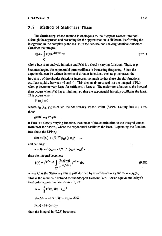
![ASYMPTOTIC METHODS 553
"~ e
-ip w eipf(z.) F(zo ) 2~ ein/4
I(p) --- ipf(z°) F(Zo) ~~ dw (9.29)
9.8 Steepest Descent Method in Two Dimensions
If the integral to be evaluatedasymptoticallyis a doubleintegral of the form:
I= ~ ~ F(u,v)ePf(u’V)dudv (9.30)
then one can follow a similar approachto Section 9.4. Thesaddle pointin the double-
complexspace is given by:
3f 0 and 3f
whichdefines the location of saddle point(s) (us,vs) in the doublecomplex
space.
Expanding
the function f(u,v) aboutthe saddle point us,vs by a Taylorseries, and
neglecting terms higher than quadratic terms, one obtains:
f(u,v)
1 2
= f(us,vs)+-~[all(U-Us) + 2a12(U-Us)(V-Vs)+a22(v-vs)2]+...
Making
a transformation about (Us,Vs) such that:
½[blX2+ b2y2] = f(Us,Vs)-f(u,v)
results in the transformation:
all (u - Us)2 +2 al2(U- UsXv s )+ a22
(v- vs )2 = _
blX2 _ b
2y
whichis madepossible by finding the transformation:
u- us = rllX + rl2Y
v- vs = r21x + r22Y
wherethe matrixrij is a rotation matrix, withr12 = -r21. Thus:
dx dy
I= ~ ~ e@(U’")-b’x’t2-b2Y’/2l
P(x,y)(dx/du)(dy/dv) (9.31)
Expanding
the integrand into a doubleTaylorseries:
P(x,y)= Fnmx2n+2v y2m+2~
(dx/du)(dy/dv) m= 0 n
wherev and2, result fromthe derivative transformations,then one canintegrate the series
term by term, resulting in the asymptoticseries:](https://image.slidesharecdn.com/advancedmathematicalmethodsinscienceandengineering-hayek-230318001731-2b30ece5/85/advanced-mathematical-methods-in-science-and-engineering-hayek-pdf-560-638.jpg)
![CHAPTER 9 556
providedthat Reb
2 > 0, or equivalently -~t/4 < arg b < ~t/4, and:
A(b,19)
-ob2,2 .
=e [B(b,0)-,~a erf(-ib~/-~)] (9.40)
Tofind B(b,0), let 19= 0 in eqs. (9.36) and(9.40), so
~ dy 1 1
A(b,0)=B(b,0)=ab yS_-b2 =a y-b dy
=alo~Y-b~ =_a Lim lo~Y- b~
~y+b) 0 y~0 .~y+b)
=~iga 0<argb<g/4 or 0<argb2 <g/2
(-i~a ~ / 4 < arg b < 0 or - n / 2 <arg b2 < 0
Thus:
A(b, 9) = ~ P 1 - eft -ib for 0 < arg b < ~/4
A (b,~) = -~ P l+eff -ib for -~/4 < arg b < 0 (9.41)
whereP is the residue of the function Aat y - b in (9.36) givenby:
P = 2nia e
-pb~
/2 (9.42)
Thetwoexpressions given in (9.41) can be written in one form as:
A(b, 0)= ~effc (-ibm) - P H(-arg 2) (9.43)
wherearg b2 wassubstituted for arg b, since both ~e equivalent. Thus,the asymptotic
series givenby eq. (9.35) is givenin full by:
I-cOl(z°) effc(-ib~)-PH(-argb2)+~ ~=0Z g2n 0n~ii[/ (9.44)
If [b[ ~ >>1, then the first order approximation
of the asymptoticvalueof eq. (9.44)
becomes:
I ~ ~ e°f(~,)(-& + g,q = .~ e°f(Zo)G(0)for IbiS>> 1
~o k b ")
Felsen
andMarcuvi~
presenta different metko~
of evaluationof tke i~tegral for B(b,~)
eq. (9.30). St~ingwith eq. (9.36) and(9.20):
~ e_9(y~_bZ)/2
B(b’o) : e ob=/2A(b’D) = ab I y2_b2
then one can express the denominator
as an integral as:](https://image.slidesharecdn.com/advancedmathematicalmethodsinscienceandengineering-hayek-230318001731-2b30ece5/85/advanced-mathematical-methods-in-science-and-engineering-hayek-pdf-563-638.jpg)
![ASYMPTOTIC METHODS 559
A_
2 : -2x/~ -Y-i~bpe-0b~ ‘2erfc (-Y-ib.~’): -2~ -pb 1 (9.55)
Likewise, A.3, A.4, etc. can be computed
by a similar procedure. It shouldbe noted that
if Ibl~>>1, then the asymptoticvalue of erfc (x) gives:
2~1
A_
2 --~
b2
whichis of the sameorder as A_
1 given in eq. (9.45).
9.11 Solution of Ordinary Differential Equations for Large
Arguments
In chapter 2, the solution of ordinarydifferential equationsfor small arguments
was
presented by use of ascendingpowerseries: the Taylorseries for an expansionabout a
regular point or the Frobeniusseries for an expansionabouta regular singular point.
Bothof these series solutions convergefast if the series is evaluatednear the expansion
point. Toobtain solutions of ordinary differential equations for large arguments,one
needsto obtain solutions in a descendingpowerseries. Toaccomplishthis, a
transformationof the independentvariable ~ =1/x is performed
on the differential equation
and a series solution in ascendingpowerof ~.
9.12 Classification of Points at Infinity
Toclassify points at infinity, onecan transformthe independent
variable x to ~, so
that x = ,,o mapsinto ~ = 0. Letting~ = I/x, the differential equation(2.4) transformsto:
d2y~ [2~-al(1/~)]dy . a2(1/~)
(9.56)
d~2 ~2 d~~"
Classification of the point ~ = 0 dependsonthe functions al(x) and a2(x):
(i) ~ =0 is a Regularpoint if:
al(x) = 2x-1+ p_2
x-2 + p_3
x-3 + ...
a2(x)= q_4
x-4 + q_sx
-5 +q_6
x-6 +...
Thesolution for a regular point then becomesa Taylorsolution:
OO OO
y(~)= ~ an~
n or y(x)= ~ x-n
n=0 n=0
whichis a descendingpowerseries valid for large x.](https://image.slidesharecdn.com/advancedmathematicalmethodsinscienceandengineering-hayek-230318001731-2b30ece5/85/advanced-mathematical-methods-in-science-and-engineering-hayek-pdf-566-638.jpg)
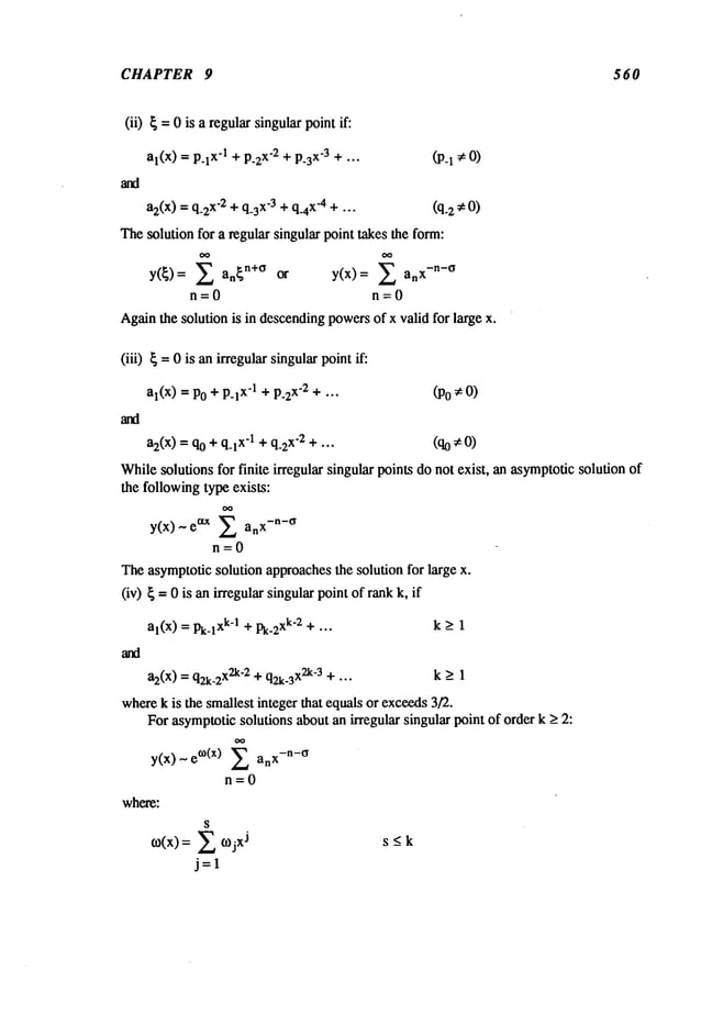
![ASYMPTOTIC METHODS 561
Example9.~i Classify the point ~ =O for the following differential equations
(i) Legendre’sequation
(1 - 2)y’’-2x y’ +n(n +
1)y =
-2x n(n + 1)
al(x) a2(x) =
l_x
2 1-x
2
n
al(x ) 2 1 2 ,~ (~1"] 2
x 1-X~x n_/~_ot.X2.) =7"i-x
-’-~"
n
a2(x)=
x2i(ln+l)
- n(n+l)
)_,j/x~) x
2
= ~
This means
that ~ = 0 is a regular singular point
n(n+l) n(n+l)
x2 x
4
(ii) Bessel’sequation
x2y,,+xy, +(x2 _ p2)y =
_ _p2
al(x) =xl a2(x) =
This indicates the point { = 0 is an irregular singular point of rankk = 1.
9.13 Solutions of Ordinary Differential Equations with
Regular Singular Points
If the point ~ = 0 is a regular singular point, then onemaysubstitute the Frobenius
solution havingthe form:
Y(~)= Z an~n+~
n=0
y(x)= Z anx-n-o
n=0
Example 9.7
Obtainthe solution for large argumentsof Legendre’sequation:
(1 - x2)y"-2x ’ +n(n +1)y =
Thepoint ~ = 0 is RSP,then assuminga Frobenius solution, one obtains](https://image.slidesharecdn.com/advancedmathematicalmethodsinscienceandengineering-hayek-230318001731-2b30ece5/85/advanced-mathematical-methods-in-science-and-engineering-hayek-pdf-568-638.jpg)
![CHAPTER 9 562
For
-ao(o + n)(o - n - 1)x-° - al[(O + n + 1)(o - n)]x
-°-1
+ E [-(°+m+n+2)(°+m-n+l)am+2+(°+m)(°+m+l)am]
x- m- °-:z=0
m=0
ao#0 Ol=-n or2 =n+l
aI =0
(or +m)(cr+m+
am+2= (o+ m+ n + 2)(0 + m- n + am m= 0,1,2...
For~r1 = -n, the fh’st solution’s coefficientsare:
(m- n)(m - n +
am+2= (m + 2)(m - 2n + am
n(n-1)
a2 = 2(2n-1) a° a4 =
n(n- 1)-.... (n -
a6 = 233! (2n- 1)(2n- 3)(2n- a°
m=0,1,2....
n(n - 1)(n - 2)(n o
222! (2n - 1)(2n-
whenm= n, an+
2 = 0 and hence an+
4 = an+
6 = ... = 0. Therefore:
I n(n-1) x-2+n(n-1)(n-2)(n-3)x
-4 ] >1
Yl=a0 x+n 1 2"~n--~ ~ii~n-~)(-~n--"~ -b .... -b( )X
-n
It can be shown
that Yl is a polynomialof degreen, whichis also identical to Pn(x).
Hence,
it is valid for all x.
For o2 -- n + 1, the secondsolution’s coefficients are:
(m+n+l)(m+n+2)
am+2= (n+2)(m+2n+3) am
(n+l)(n+2)
a2 = 2(2n + 3)
(n+1).....(n+
a6 = 233! (2n + 3)(2n + 5)(2n
Thesecondsolution can thus be written as
=a0 x_n_lF1
+ (n +1)(n 2)x_2
-~
Y2
2(2n + 3)
m=0,1,2....
(n +1)(n +2)(n + 3)(n
a4 = a
o
222! (2n + 3)(2n+
a
o
(n+l).,...(n+4) x-_4+.,.,]
222! (2n + 3)(2n+
Thesecondsolution shouldbe the representation for Qn(x)for Ixl > 1. Letting:
n!
a 0 =
1.3.5.....(2n+ 1)
results in a descendingpowerseries solution for Qn(x)for x >
x>l](https://image.slidesharecdn.com/advancedmathematicalmethodsinscienceandengineering-hayek-230318001731-2b30ece5/85/advanced-mathematical-methods-in-science-and-engineering-hayek-pdf-569-638.jpg)

![CHAPTER 9 564
(~2 +Qo) an +[Q1-2~(~ + n-l)] an-1 +[Q2 +6+n-2]an-2
k=n
+ E Qk an-k =0
k=3
If Q0* 0, then for n = 0:
(o)2 +Qo)a0
sincea0 ;~ 0, then:
o)2 + Qo= 0
o)1 = i~o o)2 = -i~o (9.60a)
Thismeansthat the first term of eq. (9.60a) vanishesfor all n when
o) is equal to COl
¢oz. Forn=l:
[Q1 - 2~] a0 = 0
whichresults in the valuefor ¢r since a0 ~ 0
~= Q~I or ~1 = Q~I and if2-Q1 (9.60b)
2o) 2o) 1 2o)
2
For n = 2:
(Q2 + ~Yl,2 )
a1 = a
o
2o)1,2
Forn>_3: with¢Yl,¢r2, o)l, o)2 givenabove,the recurrenceformulabecome.,;:
n
2o)l,2(n-1)an-1 =[Q2+CYl,2+n-2] an-2+ E Qk an-k n>3 (9.61)
k=3
It should be noted that both normalsolutions are called FormalSolutions, i.e. they
satisfy the differential equation,but the resulting series in general diverge. However,
these solutions represent the asymptoticsolutions for large argumentx.
Example9.8 Asymptotic solutions of Bessel’s equation
Obtainthe asymptoticsolutions for Bessel’s equationof zero order satisfying:
y"+ly’+y = 0
This equation wasshownto have an irregular singular point of order k = 1. Transforming
y(x) to u(x) the ordinarydifferential equationbecomes:
y =x-~u(x)
u"+ 1+ u=0
Here Qo=1, Q1=0, Q2= 1/4, and Q3= Q4..... O.](https://image.slidesharecdn.com/advancedmathematicalmethodsinscienceandengineering-hayek-230318001731-2b30ece5/85/advanced-mathematical-methods-in-science-and-engineering-hayek-pdf-571-638.jpg)
![ASYMPTOTIC METHODS 565
Thus:
o~2 = -1 co1 = +i 60
2 = -i ffl =0
1 (¼+n_2)an_2
al_ ~-_
1 and
an_1 =
2co 86o’ 2~o(n- 1)
Therefore, the succeedingcoefficients become:
(I. 3)
2
a2=2!82~o
-~---~-
a°
(1.3.5)
2
a3 = 3!83~o3 a°""
and by induction
[1.3.5 ..... (2n - 1)]
2
an =
8n n[ 6o
n a°
[½.3 5 2~_-1] 2 [[’(n + ½)]
2
a 0 =
2n n!o)
n
F2(½)2n n!to
n
_ ao
~t 2n ton n!
~2=0
n>3
n=l,2......
a0
Thetwo asymptoticsolutions of Bessers equation are:
e+iX
oo
1-’2(n + ½) -n
Yl,2 - ~x a° Z (’T-i)n n n! x
n=0
Choosinga0 = 2~" ey-in/4, then the asymptoticsolutions are those for H(01)(x)
H(o2)
(x), i.e.:
Ho(1)(x) - 2 ei(X_Zff4 ) Z ~
n!
n=0
~- ~.~0( ")n F2(n+½)
Ho(2)(x) ~ ~ e_i(x_n/4)
1
~rrx ~x n!
Examination
of the asymptoticseries for H(01)(x)and H(02)(x)showsthat the
should be summed
up to N terms, provided that x > N/2.
9.14.2 Subnormal Solutions
If the series for Q.(x) happensto haveQo= 0, then (Yl,2 become
unbounded.
To
overcome
this problem,one can performa transformation on the independentvariable x:
Let ~=X½, X= ~2 and rl = ~-½u(~) = x-¼u(x) whichresults in a newordinary
differential equationonrl(~):](https://image.slidesharecdn.com/advancedmathematicalmethodsinscienceandengineering-hayek-230318001731-2b30ece5/85/advanced-mathematical-methods-in-science-and-engineering-hayek-pdf-572-638.jpg)
![CHAPTER 9 566
where:
P(~) = 4~2Q(~2)- +
If Qo= O, and Q1~ O, then:
Q(x) = x-1 + Q2
x-2 + .. .
(9.62)
Q(~2) = Ql~-2 + Q2~-4+ Q3~-6+ ...
sothat:
P(~) = 4Q1+ (4Q2--~] ~-2 + -4 +.. .
Here:
Po(~) : 4QI
PI(~)=
3
P2(~) = 4Q2
P~=O
P4(~) = 4Q3
Now,one canuse the normalsolution for an irregular point of rank oneon rl(~), i.e., let:
n({)~e~ 2 an{-n-~ (9.63)
n=0
so that:
u(x) ~ 1/4 e~ Zanx-( n+~)/2
n=0
Since PO= 4 Q1,then:
o32 = Po = -4QI
~=~=0
o31,2
---- -+2i,~’~
so that:
u(x) ~ ~°4~ 2anxl/ 4-n/2
n=O
Again, the subnormal solutions are FormalSolutions as they satisfy the
differential equation,but are divergentseries.](https://image.slidesharecdn.com/advancedmathematicalmethodsinscienceandengineering-hayek-230318001731-2b30ece5/85/advanced-mathematical-methods-in-science-and-engineering-hayek-pdf-573-638.jpg)
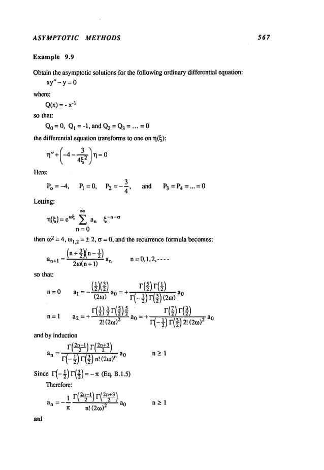
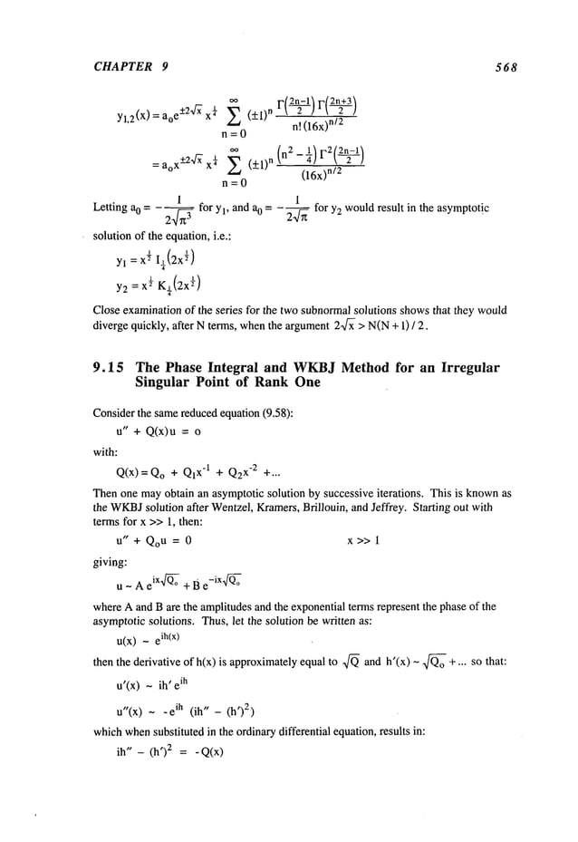
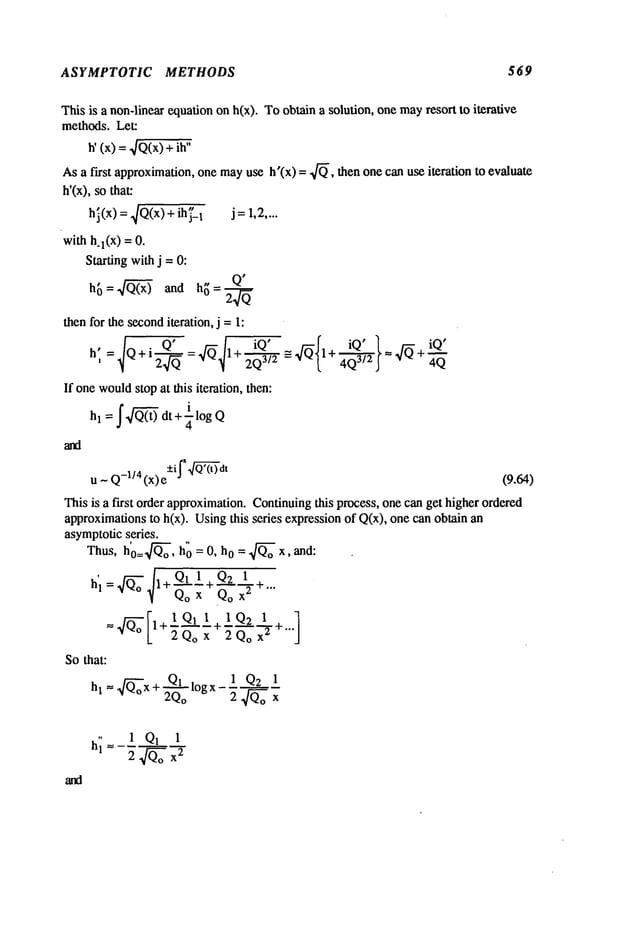
![CHAPTER 9 570
l _~ Q2 i QI 1
h2 = Qo+ -~ x2 2 ~o x2 ~’’’"
l Q1 l+(Q2 i Q1 ]~1 +
=~o 1+~o’o~ [,~oo 20o3/2)x 2 "’"
-~{1 !~QI~+=~4Q2-2i Q1 Q~] 1 }
+~l~o;X 8~oL ~ NJg
+’ ’"
~en:
~(x~- ~x + ~ f~log x- ~[4~- 2i Q1 Q~
so ~at:
Ul(X) - e~(~) _ (x)iQ,/~ ~ e+i~ x
u2(x ) - (x) -iQ,/~ e-i~ x e-iMs~
1
whe~ A- ~4Q2 2iQ1 Q~
- ~ ~ Qo)
Using eia = ~ (~)n, one obtains ~e des~ed ~pmtic series.
n=0
Example 9.10 Asymptotic solutions of Bessel~ equation
Ob~n~e ~ymp~fic solution of Bessel functions by ~e WKBJ
me~od.
~ x dx ~
y= 0
Letting y(x) = x-~/~u(x), then:
~2 ~ x2
whe~ Q = 1-~(p 2 -~), with:
(9.65)](https://image.slidesharecdn.com/advancedmathematicalmethodsinscienceandengineering-hayek-230318001731-2b30ece5/85/advanced-mathematical-methods-in-science-and-engineering-hayek-pdf-577-638.jpg)
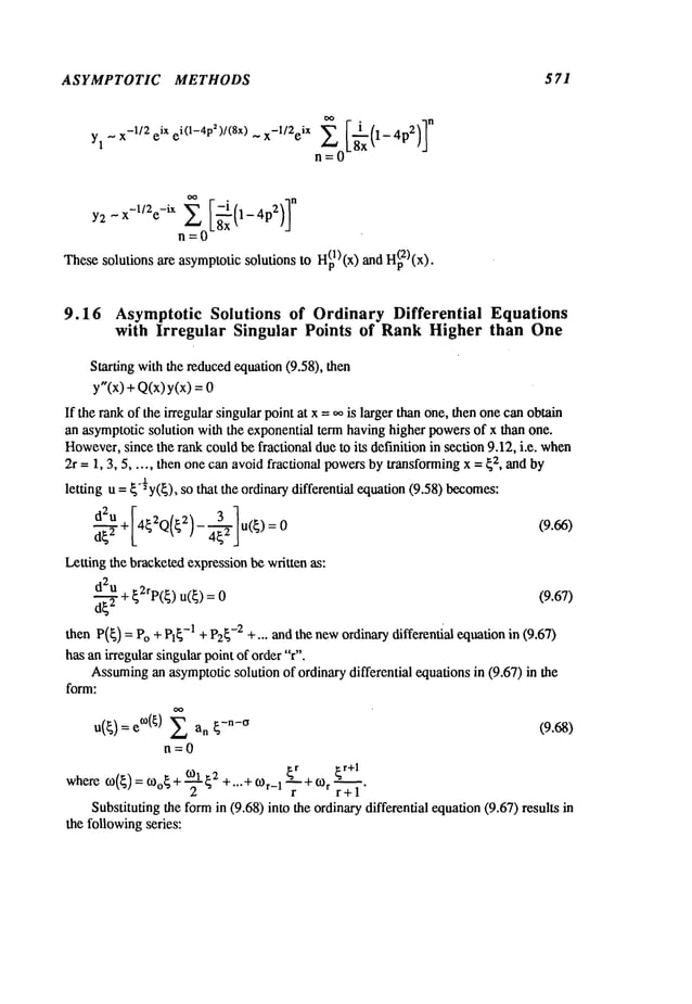
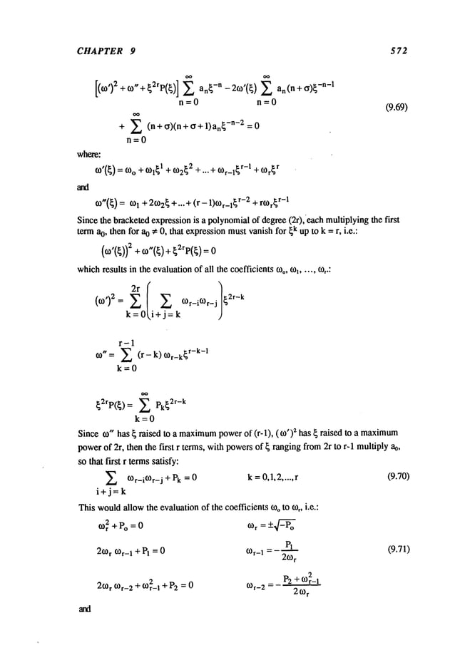
![ASYMPTOTIC METHODS 573
cr = + l~(pr+1 + r0) + 2600f0r_ 1 + 20)1 f0r_ 2 + ...)
20)r
r
Theremainingequalities in (9.69) would
determinethe series coefficients ai, a2 .... in
terms of %.
Example 9.11 Asymptoticsolutions for Airy’s function
Obtainthe asymptoticsolutions for Airy’sfunction satisfying:
y"- xy = 0
Theirregular singular point x = ~o is of r = 1/2. Dueto the fractional order, then the
ordinarydifferential equationsto:
d~2 + -4~4--~
Herer = 2, and:
3
P(~) =-4 6
Let:
3
P0=-4, PI=P2=P3=P4=P5=0, P6=--~, P7=P8=...=0,
u(~) : ~-l/2y(~)
Followingthe procedureoutlined in (9.71):
0)~ -4=0 0)2 =-+2
0)0=0 ~=1
0)1 =0
Thus:
~3
0), = 0) tO"
0) = 0)2 "~, 2~ = 20)2~
Substitutingthese in eq. (9.70) andthe valueof 0)2:
3 -n
E [(20)2~ - ~--~ -)an~ - 20) 2 (n + 1) an~-n+l + (n + 1)(n + 2)an~
-n-2] = 0
n=0
Expanding
these series, one finds that a~= a2 = 0, and:
(m+l)(m+2)-¼
am+3= 2(m + 3)0) 2 a m m = 0,1,2 ....
Usingthe recurrence formula, one can write the twoasymptoticsolutions as:](https://image.slidesharecdn.com/advancedmathematicalmethodsinscienceandengineering-hayek-230318001731-2b30ece5/85/advanced-mathematical-methods-in-science-and-engineering-hayek-pdf-580-638.jpg)
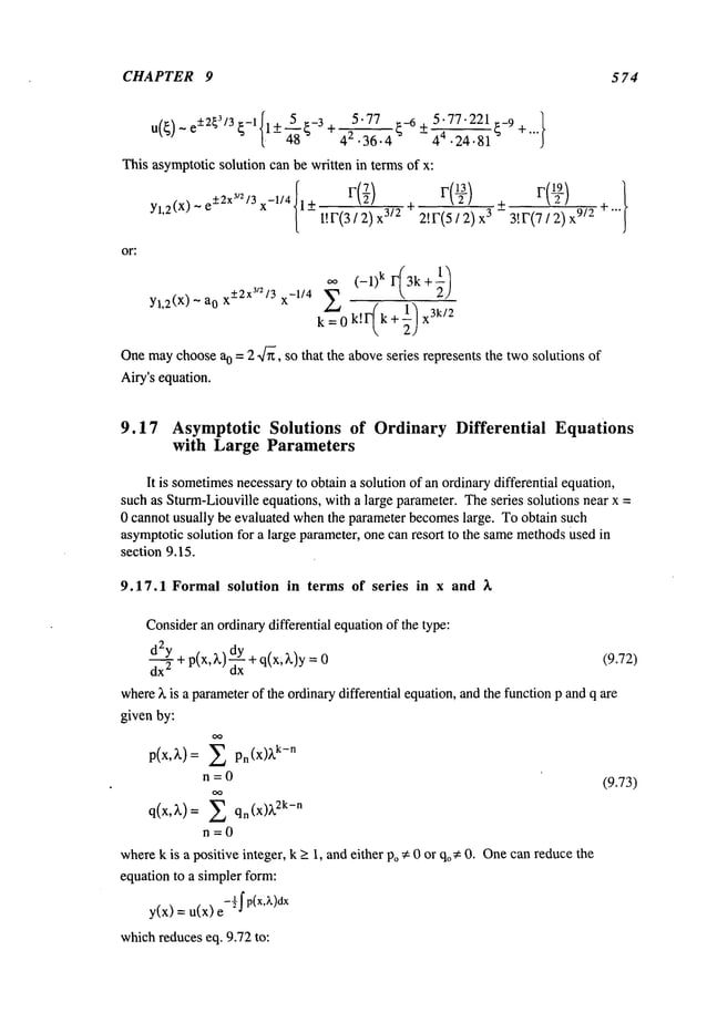
![ASYMPTOTIC METHODS 575
~ + Q(x,3.) u(x) (9.74)
dx"
whereQ(x,3.) =q(x, 3.)- ½p’(x, 3.)- ¼p2 (x, 3.)and represented by:
Q(x,3.) : ~ X 3. 2k-n (9.75)
n=0
A formalsolution of the ordinarydifferential equation(9.74) of the form:
= e°)(xA) ~ un (x) 3.-n (9.76)
u(x)
n=O
where
=
k-1
~ O)m(X) 3.k-m (9.77)
m=O
Substituting (9.77) and (9.76) into eq. (9.74), oneobtains:
k-1 ,, (k-I ,
k m"~2] ~
m=O m=O ) Jn=O
+2 / E O)m(X)3.k-m il;(x)~-n+ E UX(X)~-n (9.78)
m = ~n = 0 n = 0
Thecoefficient of )~ ~-~canbe factoredout, resulting in the recurrenceformula:
~ Un_t(x) Qz(x)+
£=0 L m=O
+ Un_~(x)m~_k +2 un_~(x)~¢_k(x) Un_2k(×)=0
g=0
Thesummation
is performedwith the proviso that :
uq=O q=-1,-2 ....
o~q=O q---l,-2 .... andq = k,k+l....
Setting n = 0 in (9.75), andsinces =0 for q = -1,- 2 .. .. then the first (k-l) termsof the
first bracketedsumof (9.79) mustvanish, i.e.:
(9.79)
n =0,1,2....](https://image.slidesharecdn.com/advancedmathematicalmethodsinscienceandengineering-hayek-230318001731-2b30ece5/85/advanced-mathematical-methods-in-science-and-engineering-hayek-pdf-582-638.jpg)
![CHAPTER 9 576
QI + Om(Ol-m = 0
m=0
setting ~ = 0 gives:
Qo
+[0;(")]
2=0
Q1
+2o~,~i
=0 or
g=O,1,2
..... k-1
~,(,,)=+-47~o(x)
Ql(X) Ql(X)
=-
2,o’-’To
=
(9.80)
or in moregeneral form:
m=g-1
2¢°o¢°t + Qt + 03mO/-m= 0
m=O
(9.81)
g=l,2 ..... k-1
g-1
o~ = m=l g=l,2..... k-1
2~o~(x)
whichgives an e,,pression for all the unknown
coefficients, i.e., o},g = 1,2 ..... k - 1 in
terms of the twovalues of c0~(x).
After removing
the first (k-l) fromthe first bracketedsumof I. (9.79), there
remains:
Un-/ l + ~0m(0/-m Un-/~/-k
m=0 J g=0
(9.83)
+2 un_t~t_ k + Un_2k= 0 n =1,2,3,...
~=o
Setting n =k in (9.83), one obtains a differential equationfor u~(x), i.e.:
2u~, CO
o + COg+ Qk + m k-m Uo = 0
m=l
resulting in a linear first order differential equationon
u~,(x) + Ao(x)Uo(X) (9.84)
where Ao(x)="~I o +Qk + Z
[
°)"2c°~’ m = 1
Defining:
I~(x)
=e-J
A*(x)a (9.85)
then the solution for u
o (eq. (1.9)) canbe written
so that: (9.82)](https://image.slidesharecdn.com/advancedmathematicalmethodsinscienceandengineering-hayek-230318001731-2b30ece5/85/advanced-mathematical-methods-in-science-and-engineering-hayek-pdf-583-638.jpg)
![ASYMPTOTIC METHODS 577
Uo(X)
=Co
Ix(x)
Similarly one canfind formulaeforun.’ ¯
un + Ao(x)Un(X)= Bn(x)
where:
Bn(x) Un-g (D~’+Qk+g+
1
"
(D~n(D[+£-m
+ 2U~-e(D}+ Un-k
m=g+l
(9.86)
whosesolution is given by eq. (1.9):
Un(X)= n IX(x) +
Ix(x)f Bn(x) dx
Ix(x)
(9.87)
Notethat except for the constant C,, the homogeneous
solution for u,(x) is the same
function Ix(x) for Uo(X).Since:
’ +-~o(1
(DO = X
then eqs. (9.82) and(9.87) yield twoindependent
solutionsfor (D~,(DE (Dk
andu0,ut .....
Example 9.12 Asymptoticsolution for Bessel Functionswith large orders
Obtainthe asymptoticsolution of Bessel functions for large argumentsand orders.
Examining
the Bessel’s eq.:
z2d2y . dy . [ 2
-S-T ~- z-- ÷ ~z -p2)y=0
dz dz
whosesolutions are Jp(z) and Yp(Z),and letting z = px, then the equationtransforms
x2__d2Y
+xd-~Y
+p2(x2
- 1)y=
dx2 ux
Thesesolutions can be expanded
for large parameterp. and large argumentpx.
Letting:
_Ifdx ~
y(x) = u(x) 2J x = X~H( X)
then the equationtransformsto:
d2u~- Q(x, p) u =
dx
2
where:
Q(x)=p2(1-~2]-~
4x
2
Thus, here:
1 1
k = 1, Qo = 1- -- Q1 = 0, Q2 - -- Q3 = Q4 = ... = 0,
x2 , - 4x
2 ’
and:](https://image.slidesharecdn.com/advancedmathematicalmethodsinscienceandengineering-hayek-230318001731-2b30ece5/85/advanced-mathematical-methods-in-science-and-engineering-hayek-pdf-584-638.jpg)
![CHAPTER 9 578
o)(x)
=pO)o(X)
Therefore:
co~, = - 1 _ x
Equation(9.84) gives:
Ao(x) = ~o
=
Ix(x) = e J2to. = (¢o~)-1/2
(l_x2)
1/’
xl/2
Uo(X)
=Co(~g)
1/: =Co
~
x:)
whe~.C~~e constant. For n = 1
.... f[-1- A~ +Ao
2 1 ]
Finding closed form solutions for u~(×) has become
an arduoustask, whichgets more
so for higher orderedexpansionfunctions u,(x). However,
one can obtain the first order
asymptoticvalues as:
Y2
~x-½
e-Plm°l
Uo(X)
- x-½
e_p
l_,]i2~x~
fi~, +~_~_~x2,)x
-P
9.17.2 Formal solutions in exponential form
Anotherformalsolution can be obtained by writing out the solution as an
exponential,i.e.:
u"+Q(x,~k)u=](https://image.slidesharecdn.com/advancedmathematicalmethodsinscienceandengineering-hayek-230318001731-2b30ece5/85/advanced-mathematical-methods-in-science-and-engineering-hayek-pdf-585-638.jpg)
![ASYMPTOTIC METHODS 5 79
Q(x,~,)= E Qn(x) ~2k-n
n=O
by use of the formal expansion:
u ~ e
o(x’x) (9.88)
where:
CO(X,~,)= E con(X)~’k-n (9.89)
n=O
Substituting eq. (9.88) into the ordinarydifferential equations,one has to satisfy the
followingequality:
co. +(co,)2 + Q= (9.90)
whichresults in the followingrecurrence formulae:
n
+ E CO~nco~t-m = 0
n = O,1,2...k- 1 (9.91)
Q.
m=O
n
n-k + ~m ~n-m + Qn = 0 n > k (9.92)
m=0
Forn =0 in (9.91) gives a valuefor coo:
Qo+ (co~,)2 co~,=+-4---~o: +i Q4"~o (9.93)
whichis the sameexpression as in (9.81):
Q1+ 2co~co~
= 0 co{ = Q1
2co~
whichis the sameexpressionas in (9.81) and in general gives:
con =-2co’--"7o’o [ E co~nco~_m+Qnj n=l,2..... k-1 (9.94)
Lm= 1
For n > k use eq. (9.91) to give
con = 2(o; COmcon-m + Qn + con-k ] n > k (9.95)
Thetwo formalsolutions (9.76) and (9.88) are identical if one wouldexpand
exponential
termsin e°~x’x)for n >k into an infinite series of k-n.](https://image.slidesharecdn.com/advancedmathematicalmethodsinscienceandengineering-hayek-230318001731-2b30ece5/85/advanced-mathematical-methods-in-science-and-engineering-hayek-pdf-586-638.jpg)
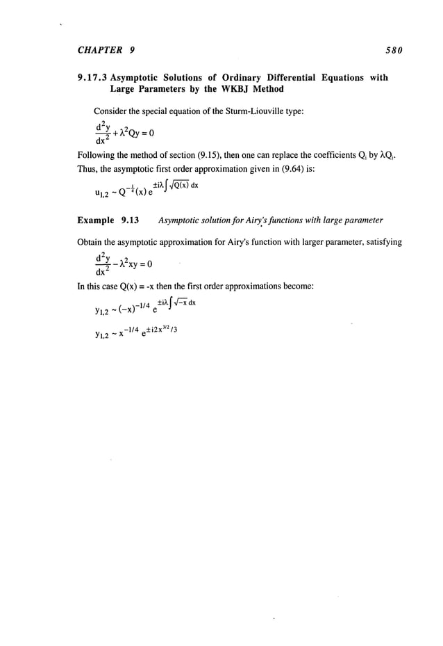
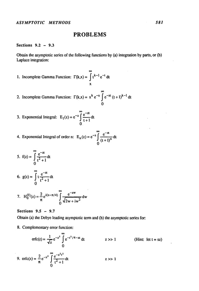
![CHAPTER 9 582
10. H(vl)(z)= -ie-iVn/2 iz/2(t+l/t) t-v-1 dt z >> 1
0
Alsof’mdJr(z) and Yv(z),where1) = Jr(z) + i Yv
(Z
~+ ig
11. e z>>
1
12. Kv(z) = e-zc°sh(t) [sinh (t)] 2v dt z >> 1 for v > 1/2
F(v
0
13. Kv(z)= --l(z--~ v ~e-t-z2/(4t)t-V-ldt z>> 1 for
22]
0
v > 1/2 (Hint: let t = zs)
14" Kv(z) =F(v~+ 1 / 2) (z)V~-
~ e-zt (t 2 - 1)v-l/2 dt z >> 1 for v > 1/2
1
e-Z2/4 oo
15. U(n,z) = l~"~(n
-I e-Zt-t2/2tn-I dt
z >> 1 n _>1
0
ze_Z2/4 oo
F(n / 2) e-t tn/~-I (z2 + 2t)-(n+~)/2 dt
0
16. U(n,z)=
eig/4 . 2 ~ e-iZ~t2
17. FresnelFunction: F(z)= --~--,~-~ze lz ! ~tdt
~ _X2t
2
. 2x -x’[ e,_.~_~tdt
18. Probability Function: ~(x) = ~- _
4t
z + 1
(Hint:let t =zs)
Section 9.13 - 9.16
Obtain the asymptoticsolution for large arguments( x >>1) of the following ordinary
differential equations
d2y 2X~x 0
19. ~-T+ =](https://image.slidesharecdn.com/advancedmathematicalmethodsinscienceandengineering-hayek-230318001731-2b30ece5/85/advanced-mathematical-methods-in-science-and-engineering-hayek-pdf-589-638.jpg)
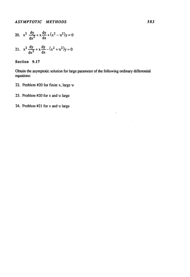
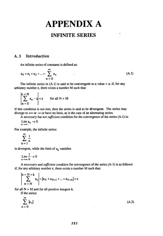
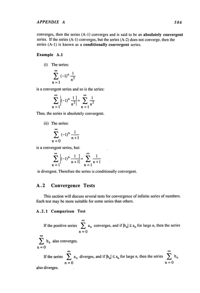
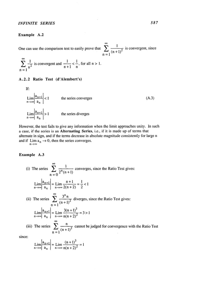
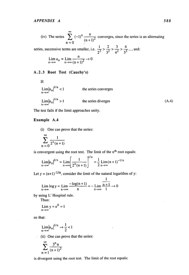
![INFINITE SERIES 589
r n -~l/n ,- -din
Lim[anl l/n = Limit/ = 3 Lim(n+ 1) -l/n Lim [---~]
n-->** n-~**L(n
+ ) J n-~** n-->**
n+1,/
From
part (i), Lira (n +-l/n =1,therefore:
n--~**
f n ,~l/n (" 1 l/n
Lim~nl 1/n = 3 Limit/ = 3 Limit/ =3>1
n~ n-~**n+lJ n->**~l+ 1/n)
A.2.4 Raabe’s Test
For a positive series {an}, if the Limit of (an+l/an) approachesunity, wherethe Ratio
Test fails, then the followingtest gives a criteria for convergence.
If:
Limln[ an _11}>1 the series converges
n -->**[Lan+l
n--->**[Lan+l
the series diverges (A.5a)
If this limit approachesunity, then the followingrefinementsof the test can be used:
Lim(logn)In [ an-1]-1}>1 the series converges
no** [ Lan+~
Lim(logn)In [ an-11-1}<1 the series diverges
n-~** [ Lan+l
If this limit approachesunity, then the followingrefinementsof the test can be used:
Lim (log n)I(logn)In [ an_ 1]-1 l- 1}>1 the series converges
n-~**
L [ Lan+l J J
Lim (logn~(lo, n)In I an-11-11-1}<1
n-~- [ t Lan+l J J
(A.5b)
the series diverges (A.5c)
If the limit approachesunity, then anothertest basedona refinementof (A.5c)can
repeatedover and over.
Example A.5
(i) The series _~ 1 could not be tested conclusively with the Ratio test,
. v= (n+ 1)
2
but it canbe tested usingRaabe’s
test:](https://image.slidesharecdn.com/advancedmathematicalmethodsinscienceandengineering-hayek-230318001731-2b30ece5/85/advanced-mathematical-methods-in-science-and-engineering-hayek-pdf-595-638.jpg)
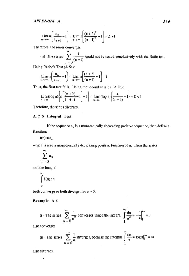
![INFINITE SERIES 591
A.3 Infinite Series of Functions of OneVariable
Aninfinite series of functions of one variable takes the followingform:
~ fn(X) a-<x<b
f0(x)+fl (x) +f2(x)
n=0
Theseries can be summed
at any point x in the interval [a,b]. If the sumof the series,
summed
for a point xo, convergesto somevalue f(xo), then the series is said to converge
to f(Xo)for a _<o _< b. Thus, i f one chooses a
n arbitrary s mall n
umber e
, t hen there
exists a number
M,such that the remainderof the series RN(X):
n=N
f<xo)-fo<xo) N>M
n=0 I
N
f(Xo)= Lira ~ fn(Xo)
n=O
A necessaryandsufficient conditionfor convergence
of the series at a point xo is
that, givena small arbitrary number
e, then there exists a number
M,such that:
for all N> Mandfor all valuesof the positive integer k.
It should be noted that the sumof a series whoseterms are continuousmaynot be
continuous.Thus,if the series is convergentto fix), then:
N
~ f.(x)-~ f(x)
Lira
n=O
t[
N
] fh(
x
)
f(Xo)= Lim f(x)= Lira Lim (A.6)
X-~).X
o
x-’X°LN-’~*
n =O
Onthe other hand, by definition:
f(x~) = Lim ~’. Lim fn(x)
N--~,~[ ~ x-~x,
Ln=0
Thelimiting valuesfor f(xo) as given in (A.6) and(A.7) are not the sameif is
discontinuousat x = xo, they are identical onlyif f(x) is continuousat x = Xo"
n=N+k |
IfN(x)
+fr~+,(x)+ + fN+k(x~: ~ fn(X~ <
n=N 1](https://image.slidesharecdn.com/advancedmathematicalmethodsinscienceandengineering-hayek-230318001731-2b30ece5/85/advanced-mathematical-methods-in-science-and-engineering-hayek-pdf-597-638.jpg)
![APPENDIX A 592
A.3.1 Uniform Convergence
Aseries is said to convergeuniformlyfor all values of x in [a,b], if for any
arbitrary positive number,there exists a number
Mindependentof x, such that:
f(x) fn(X) < for N > M
n=0
for a/l valuesof x in the interval [a,b].
Example A.7
Theseries of functions:
(1 - X) + X(1 - X) x2
(1 - x)...
can be representedby a series of fn(x) given by:
fn (x) =n-1 (1 -x) n =1, 2, 3 ....
Summing
the first Nterms, one obtains:
N
E fn (x) = 1
X
N
n=l
Thesedes convergesfor N-> oo iff:
Ix[<l
Therefore,the sumof the infinite series as N--) o~approaches:
I]
f(x) = Lim~". fn (x) for Ixl <1
Thus,to test the convergence
of the series, the remainderof the series RN(X)
is found
to be:
which
vanishesas N"--) ~, onlyif Ixl < 1.
For uniform convergence:
[xN[< E for e fixed and for all N> M
I I
N> ilog(ixD
[
If one choosesan e = e1°, then one mustchoosea value N such that:](https://image.slidesharecdn.com/advancedmathematicalmethodsinscienceandengineering-hayek-230318001731-2b30ece5/85/advanced-mathematical-methods-in-science-and-engineering-hayek-pdf-598-638.jpg)
![INFINITE SERIES 593
10
N>
IlogOxl)l
Thus,the series is uniformlyconvergentfor 0 _<x < xo, 0 < xo < 1. At the point x = x
o
choose:
10
N=
logOxoO
Asthe point xo approaches1, Ilog Xol--) 0, andone needsincreasingly larger and larger
values of N, so that the inequality Rn < e cannotbe satisfied by one value of N. Thus,
the series is uniformlyconvergentin the region 0 _<x _<Xo,and not uniformlyconvergent
in the region0 _<x _<1.
A.3.2 Weierstrass’s Test for Uniform Convergence
Theseries fo(X)+fl(x) +.... converges
uniformlyin [a,b] if there exists a convergent
positive series of positive real numbersM
1 + M
2 + ... such that:
[fn (x~ _< n for a ll x in [a,b]
Example A.8
Theseries:
1
X n2+x
2
n=l
convergesuniformlyfor _oo< x < oo since:
Ifn (x)l = -< n’~ Mn
andsince the series of constants:
Mn= 1 converges
n=l 1
for all x _>0
A.3.3 Consequences of Uniform Convergence
Uniform
convergence
of an infinite series of functions implies that:
1. If the functions fn(x) are continuousin [a,b] andif the series convergesuniformly
in [a,b] to f(x), then f(x) is a continuous
functionin [a,b].
2. If the functionsfn(X)are continuousin [a,b] and if the series converges
uniformlyin [a,b] to f(x), then the series can be integrated termby term:](https://image.slidesharecdn.com/advancedmathematicalmethodsinscienceandengineering-hayek-230318001731-2b30ece5/85/advanced-mathematical-methods-in-science-and-engineering-hayek-pdf-599-638.jpg)
![APPENDIX A 594
x2 x2 x2 ~ x2
x
I x
1 Xl n= 0 x
1
wherea _<x
1, x2 < b.
3. If the series E fn (x) convergesto f(x) in [a,b] and if each term fn(x) fn’(X)
n =0
are continuous,andif the series:
~ f~(x)
n=0
is uniformlyconvergentin [a,b], then, the series canbe differentiated term by term:
f’(x)= 2 f~(x)
n=0
A.4 Power Series
Apowerseries about a point xo, is definedas:
oo
ao + a~(x- Xo)M+ a2(x- Xo)
TM+ .... 2 an(X-
Xo)
nM (A.8)
n=0
whereMis a positive integer. Thepowerseries is a special formof an infinite series of
functions. Theseries mayconvergein a certain region.
A.4.1 Radius of Convergence
For convergence
of the series (A.8) either the Ratio Test or the RootTest can
employed. TheRatio Test gives:
Lim .an+l (x- ~)M. = Ix- xolM Lim an~l < 1 the series converges
n-->** an(X- Xo) n’->~l an I
> 1 the series diverges
or if one defines the radius of convergence
p as:
p = ILim] an [11/M
[n-~**lan+lIJ
then the convergence
of the series is decidedbythe conditions:
Ix - xol < p the series converges
(A.9)
>p the series diverges (A.10)](https://image.slidesharecdn.com/advancedmathematicalmethodsinscienceandengineering-hayek-230318001731-2b30ece5/85/advanced-mathematical-methods-in-science-and-engineering-hayek-pdf-600-638.jpg)
![INFINITE SERIES 595
In other words,the series convergesin the region:
xo - 13< x <xo + O
and divergesoutside this region.
TheRoot Test gives:
"i "~ a n (x- nM
Xo) = Ix - Xo[Limlan[
1/nM < 1 the series converges
>1 the series diverges
~’ (4-1)
3n
,,~ 33n oo 1
n27
n n27
n n
n=l n=l n=l
whichdiverges. At the secondend point, x - 1 = -3 or x = -2, and the series becomes
an
alternatingseries:
(-2--1)2n : 2 (-3)3n = ~ (-1)n
n 27n n 27n n
n=l n=l n=l
whichconverges,so that the region of convergence
of the powerseries is - 2 < x < 4.
Thus,if onelets:
(A.11)
then the series converges
in the regionindicated in (A.10).
TheRatio Test or the RootTest fails at the end points, i.e., when
]X-Xo[= 0, where
both tests give a limit of unity. In such cases, Raabe’sTest or the AlternatingSeries
Test (if appropriate)canbe usedon the series after substituting for the endpoints at x
xo +13or x = xo- 13.
Example A.9
Find the regions of convergence
of the followingpowerseries:
(x-:1
n
n27
n
n=l
Here M= 3, so that the radius of convergenceby the Ratio Test becomes:
13
:nt,i_,l(n
+_
1)27n+
1/3
n 27
n = (27)1/3 = 3
while using the Root Test:
-n -l/3n
13 = Lira 27-" = (27)1/3 Limn1/3n --~ 3
n ---).~
At one end point, x - 1 = 3 or x =4, the series becomes:](https://image.slidesharecdn.com/advancedmathematicalmethodsinscienceandengineering-hayek-230318001731-2b30ece5/85/advanced-mathematical-methods-in-science-and-engineering-hayek-pdf-601-638.jpg)
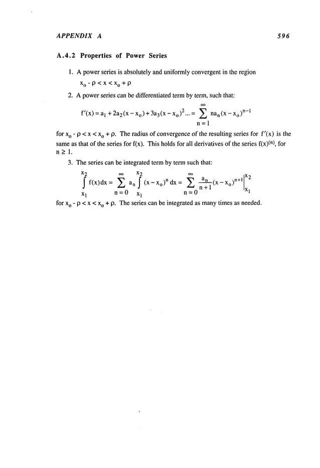
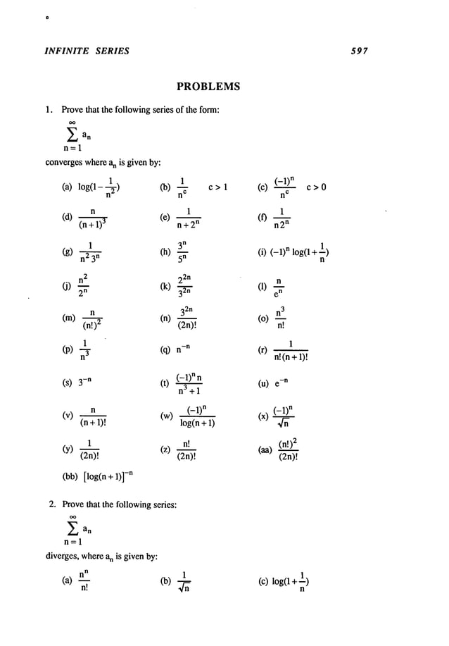
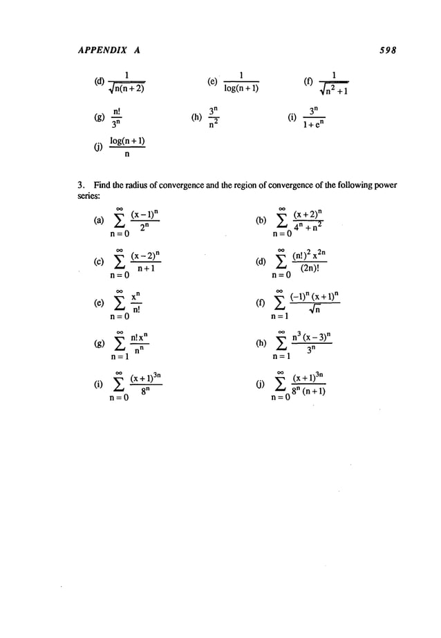
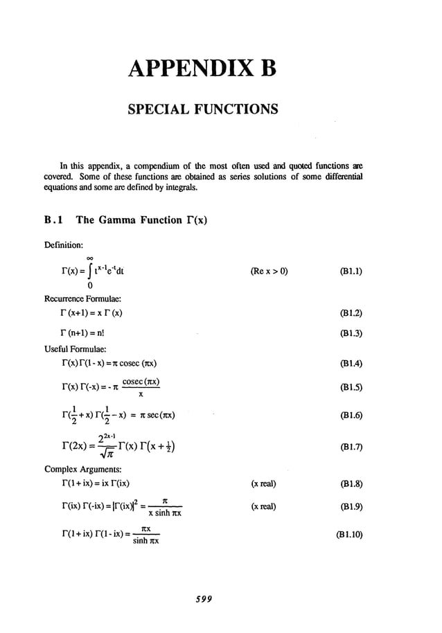
![APPENDIX B 600
Asymptotic
Series:
r(z) ~ ~ Zz’l/2 e-z 1 + + 288z-’~-
izl >>1 largzl <rc
SpecialValues:
F(1/ 2) =~l/;z
139
~1/2
F(3 / 2) =
2
r(n+½)=4~(2n’l)
tt
2
n r(½_~)__q~
(-1~
"2"
(2n- 1)!!
where
thesymbol
n!! = n (n - 2) ..... 2or
Integral Representations:
xZ
~ eixt (it)z’l dt
F(z)-- 2 sin(r~z) x>O 0 < Re(z)<
r(z) [ cos(xt) z’l dt
cos(rrz / 2),/
0
x>0 0 <Re(z)<
r(z)= sin 0rz/2) sin (xt) z’l dt
0
x>0 0 < Re(z)<
F(z)=~"t tz-1(log t) (t -z)
0
Re(z)>
F(z)=J exp[zt - et ] dt Re(z)>0
031.11)
031.13)
031.14)
031.15)
031.16)
031.17)
B.2 PSI Function q(x)
Definition:
v(z)= r(z)~](https://image.slidesharecdn.com/advancedmathematicalmethodsinscienceandengineering-hayek-230318001731-2b30ece5/85/advanced-mathematical-methods-in-science-and-engineering-hayek-pdf-606-638.jpg)
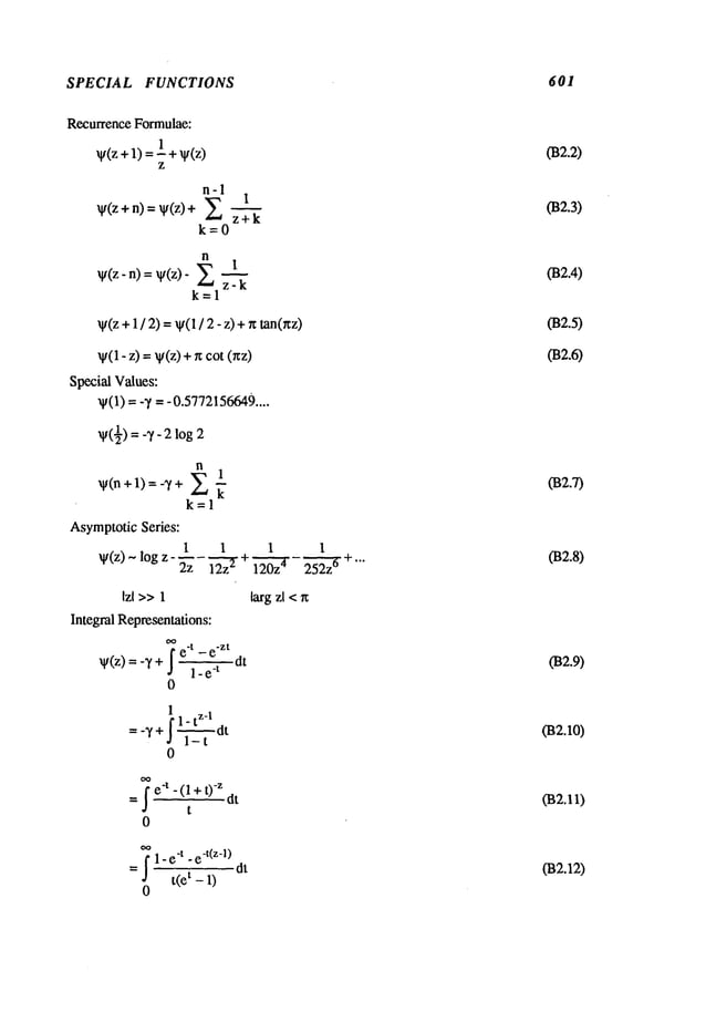
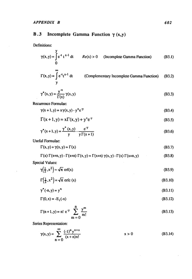
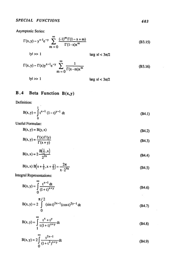
 = 2_~(_1). -x2 H
. ( x)
(B5.11)](https://image.slidesharecdn.com/advancedmathematicalmethodsinscienceandengineering-hayek-230318001731-2b30ece5/85/advanced-mathematical-methods-in-science-and-engineering-hayek-pdf-610-638.jpg)
![SPECIAL FUNCTIONS 605
~xx{erf(x)} = -x2
w
(n) (x) = -2x (n-l) -2(n - 1)(n-2) n=2,3 ....
w(°)(x) = dw -2xw(x)+
w’(x)
=-~x
~x {erfc(x)} = -xs
Integral Formulae:
’erf(x) dx = x erf(x)
- "~- ex [ b2 - cI eft(at + b a)
’exp[-(a2t 2 +2bt+c)]dt- ~ p[~-~- /
1 at a
s/4bs
’eaterf(bt)dt=~[e erf(bt)-e erf(bt-a/4b)]
’e-(at)~ e-(b/OSdt=.~ [e2aberf(at + b / t) + e-2a~erf(at_]
Sexp[-(a2t2+2bt+c)] dt = ~-~-~
exp~
ab--~-c]eff(b/
0
t" e-a tdt _.~..~ ea2X
2
j0 t+~X2= a erfc(ax)
oo 2 2
I" e-a t dt ~ ea2xs erfc(ax)
J t 2 + x2 2x
e-aterf(bt) dt = leas/4bs erfc(a/2b)
a
0
7 e-aterf(b-~) dt =
o a a+4~-~
S e-aterf(b / .~’) dt = 1_e_264~
a
0
035.12)
(B5.13)
(B5.14)
(B5.15)
(B5.16)
035.17)
035.18)
(B5.19)
(B5.20)
035.21)
035.22)
035.23)
035.24)
035.25)](https://image.slidesharecdn.com/advancedmathematicalmethodsinscienceandengineering-hayek-230318001731-2b30ece5/85/advanced-mathematical-methods-in-science-and-engineering-hayek-pdf-611-638.jpg)
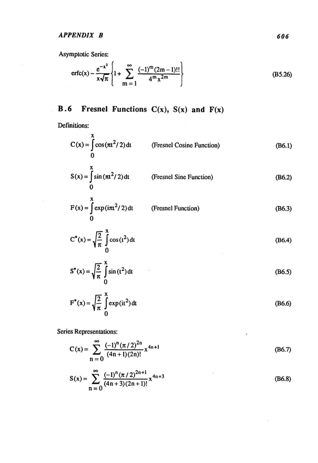
![SPECIAL FUNCTIONS 607
Useful Formulae:
C(x) = C*(x,~-~/
C(x)
=- C(-x)
COx)= i C(x)
S(x)
s(x)=- S(-x)
S(ix) = i S(x)
F (x) = ~22 ein/4erf(’~-~" e-in/4x)
Special Values:
C(0) = S(0) =
1
Lira C(x) = LimS (x)
X.’-’--~
~ X--’)’~ 2
AsymptoticSeries:
C(x) = ~ + f(x) sin(nx2/2)- g(x) cos(wx2/2)
(x) = ~- f(x) cos(xx2/2) - g(x) sin(~x2/2)
S
f(x) - ~x + m = 1 (xx2)2m
Ixl >> 1 larg xl < x/2
g(x)~~-~ (’ l)m{l’5"9"""(4m+l)}
0ZX2)
2m+l
m=0
Ixl >>1 larg xl <n/2
Integral Formulae:
IS (X)dx =x S(x) +L cos(~;x
IC(x) dx = x C(x) 1 sin(nx2/2)
f cos(a2x
2 + 2bx + c)dx = ~2 cos (b2/a2 - c)C [ 24~-(ax + b / a)]
+a-~2 sin (b2/a2 - c) S [ 2~-(ax+b / a)]
fsin(a2x2 + 2bx + c)dx = ~2 cos(b2/a2 - c) S [~-(ax + b
- ~22sin (b21 2 -c)C [2~
(ax + b / a)
F(x)F*
(x 4~-
~-)
(B6.9)
(B6.10)
({36.11)
(B6.12)
(B6.13)
036.14)
(B6.15)
(B6.16)
(B6.17)
(B6.18)
036.19)](https://image.slidesharecdn.com/advancedmathematicalmethodsinscienceandengineering-hayek-230318001731-2b30ece5/85/advanced-mathematical-methods-in-science-and-engineering-hayek-pdf-613-638.jpg)
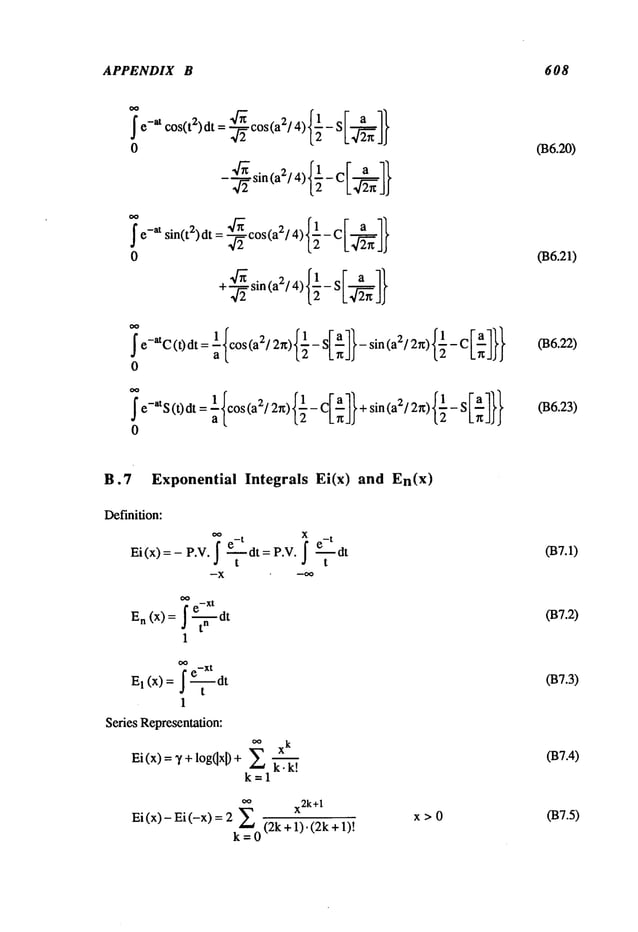
![SPECIAL FUNCTIONS 609
(-1)kx
k
E
l(x) = -y - log(x)
k. k!
k=0
En(x) = (-1) n xn [- log(x) v(n)] -
k =0,2,4
....
RecurrenceFormulae:
En+l(x) = nl-- [e-X - x En(x)
]
En(x) = - En_l(X
)
SpecialValues:
1
En(0 ) = ~
n-1
e-X
Eo(x) = ~
x
Asymptotic
Series:
Ei(x)-eX E
n=0
n!
xn+l
oo (_l)n !
El(X) ~ e-X xn +l
n=O
e-x { n(n + 1) n(n+ 1)(n +
En(x)~- ~- l-n+ -:~
x
3
x
Integral Formulae:
Ei (x)= -x f t co
s(t) + xsin(t) dt
x2 + t
2
0
= _e_X
~ t cos(t)- x sin(t)
x-
~~t-
~
dt
0
^-x7 e-t _,.
El(X)=~ j~ut
t+x
-x f t- ix it
El(X)= e j tz-~-~-x2e
0
(’l)kxk k. n - 1
(k-n+l).k!
n=1,2,3 ....
n=1,2,3 ....
n_>2
x>> I
x>> 1
+ ...} x >>1
x>0
x<0
x>0
x>0
(B7.6)
037.7)
037.8)
037.9)
037.10)
037.11)
037.12)
037.13)
037114)
037.15)
037.16)](https://image.slidesharecdn.com/advancedmathematicalmethodsinscienceandengineering-hayek-230318001731-2b30ece5/85/advanced-mathematical-methods-in-science-and-engineering-hayek-pdf-615-638.jpg)
![APPENDIX B 610
~
En(t)e
-xt dt = (-1)n----~l
X
n
o
I
log(x +1) X> -1
x
fEi (-t) t dt =- log(x) - T+eX
Ei (-
0
x
~ Ei (-at)e -bt dt= -~ {e-bXEi(-ax) - Ei (-x(a + b))+ log0+b/a)}
0
037.17)
(B7.18)
B.8
Definitions:
X
0
x
(x) =~/+log(x) +-[ cos(t)
Ci
t
0
si(x) =Si(x) - r~
Series Representations:
n~O (’l)n x2n+l
Si(x)= = (2n+l)(2n+l)!
Ci(x)=’/+log(x)+ (- 1)nx2n
n = 1 (2n) (2n)!
Useful Formulae:
Si (-x) =- Si (x)
Ci (-x) = Ci (x)
si (x) +si (-x) =
Ci (x) - Ci (x exp[irr]) = Ei (-in)
Ci (x) - i si (x) =Ei
Special Values:
si (oo)= Si (oo)
Si (0) = Ci(0) =- oo
Sine and Cosine Integrals Si(x) and Ci(x)
Ci(~)=0
038.1)
038.2)
038.3)
038.4)
038.5)
038.6)
038.7)](https://image.slidesharecdn.com/advancedmathematicalmethodsinscienceandengineering-hayek-230318001731-2b30ece5/85/advanced-mathematical-methods-in-science-and-engineering-hayek-pdf-616-638.jpg)
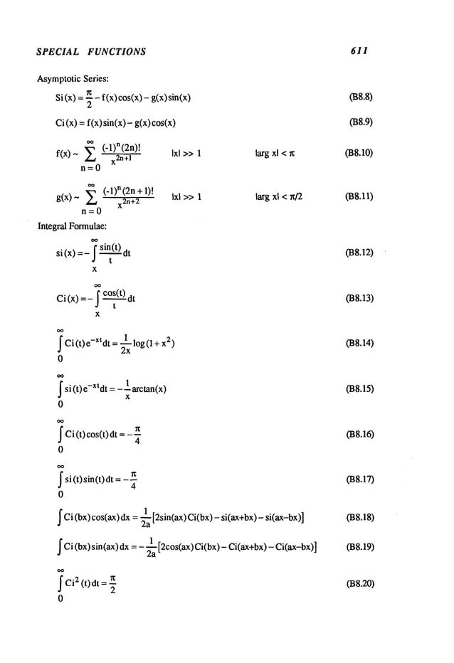
![APPENDIX B 612
$ si2 (t)dt =
0
~
Ci(t)si(t)dt log2
0
(B8.21)
038.22)
B.9 Tchebyshev Polynomials Tn(x) and Un(x)
SeriesRepresentation:
n ~21 (" -lm)~nn~m) ll) ! (2x)n -2m 039.1)
T
n (X) = "~" _
whichis the Tchebyshev
Polynomial
of the first kind. The[n/2] denotesthe largest
integerwhich
is less than(n/2).
In/2]
Un(x)= E (-1)re(n-m)!
~.~("~-~’~! (2x)n-2m
n > 1 039.2)
m=0
whichis the Tchebyshev
functionsof the secondkind.
DifferentialEquations:
(1 - 2)T~’(x)
-xT
~ (x
) + n2
Tn (x
) = 039.3)
(1 - x2) U~(x) 3x
U~
(x)+ n(n+ U
n (x) = 039.4)
RecurrenceFormulae:
T.+dx)
=2xTn(x)-
T..~(x) 039.5)
Un+1 (x) = 2xU
n (x) - n_l(x) 039.6)
(1 - 2) T
~ (x) =
- nxn(x)+ nn_
l (x) 039.7)
(1 - x2) U~(x) = - n x n (x) +(n1)U
n.1 (x) 039.8)
Orthogonality:
1
f (1 _x2)_1/2
Tn(x)Tm
(x) dx
n#m
I~n~/2 n=m
-1
039.9)](https://image.slidesharecdn.com/advancedmathematicalmethodsinscienceandengineering-hayek-230318001731-2b30ece5/85/advanced-mathematical-methods-in-science-and-engineering-hayek-pdf-618-638.jpg)
![SPECIAL FUNCTIONS 613
1
~ (1- x2)l/2Un(x)Um(x)dx
= {0r~/2 # m
-1
Special Values:
Tn(-X
) = (-1)nTn(x)
T0(x) = 1 TI(X) = x
Tn(1) = 1 Tn (-1) = n
Un(-X
) = (-1)nUn(x)
UO
(x) =
Un(1) = n+l
Other forms:
X = COS0
d~2Y+n2y = 0
T
n (cos 0) = cos(n0)
sin [(n +1)0]
Un (COS0)
sin 0
Relationshipto other functions:
T2(x
) = 2x2 - 1
T2n(0) = (-1)
n
039.10)
T
3 (x) =3 - 3x
T2n+l(0
) =0
Ul(x) = 2x U
2 = 4x2 - 1 U3(x
) = 8x
3 - 4x
U2.(0 ) = (-1) n U2n+l(0) = 039.11)
1
Tn+l(X)= x Un(X
) - Un.l(X) = "~ [Un+l(X)- Un.l(X)]
1
Un(X) = ~ [x Tn+l(X ) - Tn+2(x
)]
B.10 Laguerre Polynomials Ln(x)
Series Representation:
n
_, ~’~ (-1)rex
m
Ln(x)=n: ~,
~-’~-~ !
m=0(m.) (n-
Differential Equation:
xy"+(1 - x)y" + ny =
039.12)
(B9.13)
039.14)
0310.1)
0310.2)](https://image.slidesharecdn.com/advancedmathematicalmethodsinscienceandengineering-hayek-230318001731-2b30ece5/85/advanced-mathematical-methods-in-science-and-engineering-hayek-pdf-619-638.jpg)
![APPENDIX B 614
RecurrenceFormulae:
(n+ 1)Ln÷
1(x)= ( 1+2n- n(x)- nL
n.1(x)
xL
h (x) -- n[L
n(x)- Ln-l(x)]
Orthogonality:
I e-XLn(x)Lm(x)dx= {~n=m
0
SpecialValues:
Ln(0
) = 1
L0(x)=
L~(0)=
Ll(X)= 1-
L3(x
) = o~(X
3 - 9x2 + 18x- 6)
Integral Formulae:
I e-XxmLn(x)dx
= (-1)n n!Snm
0
I e-tLn(t) dt =-x [Ln (
x)- L
n4 (
x
I
e_XtLn(t)dt = (x- 1)
n
xn+l
0
L2(x
) = ~(x2 - 4x + 2)
x>0
0310.3)
0310.4)
0310.5)
0310.6)
03o.7)
031o.8)
0310.9)
B.I1 Associated Laguerre Polynomials Lnm(x)
Series Representation:
n
(_l)kxk
LI~(×) (n
(n- k)!(m
k--O
n,m=0, 1,2 ....
Lmn
(x) = (-1)mdmLn+m(x)
dx
m
DifferentialEquation:
xy"+(m+ 1-x)y’+ny =
RecurrenceFormulae:
(n + 1)Lmn+l(x) = + 2
n+ m
- x)L
~ (x)
- (n + m
)L
mn_l (x)
0311.1)
0311.2)
0311.3)
(Bll.4)](https://image.slidesharecdn.com/advancedmathematicalmethodsinscienceandengineering-hayek-230318001731-2b30ece5/85/advanced-mathematical-methods-in-science-and-engineering-hayek-pdf-620-638.jpg)
![SPECIAL FUNCTIONS 615
x (L~)" (x) = nL~(x)- (n 1 (x) (B11.5)
xL~+l(x)-- (x- n)L~(x) + (n + m)L~_l (B11.6)
Orthogonality:
OO
~ e_XxmLmn
(x)L~(x)dx = (n+ m)! ~0 (B11.7)
n! [1 k=m
0
If mis not an integer, i.e. m= v > -1, then the formulaegiven aboveare correct provided
one substitutes v for mand F (v + n +1)instead of (m+ n)! wheren is an integer,
Special Values:
Lm.(0) =(n +
m!n!
Integral Formulae:
~ e-ULmn
(u) du= e’X[Lmn
(x) - L~_l(X)]
x
(Bll.8)
(Bll.9)
~e-XxV+l[Ln(x)] 2n+V+lF(n+v+l)
n!
0
v>-I (Bll.10)
x
j
’tv (x - t) a LVn
(t)dt r(n + v + 1)r(a + 1).v+a+l. v+a
+l,_,
F(n + v + a + 2)
Ln tx~
0
v,a > -1 (Bl1.11)
B.12 Hermite Polynomials Hn(x)
Series Representation:
[n / 2] (.1)
m
Hn(x)=n! E m!(n-2m)!
m=O
(2x) n-2m 0312.1)
Differential Equation:
y" - 2xy"+ 2ny=0 0312.2)
Recurrence Formulae:
Hn+
1 (x) = 2xH
n (x) - 2nHn_
l(x)
H
i (x) = 2nn_l (x)
(B12.3)
0312.4)](https://image.slidesharecdn.com/advancedmathematicalmethodsinscienceandengineering-hayek-230318001731-2b30ece5/85/advanced-mathematical-methods-in-science-and-engineering-hayek-pdf-621-638.jpg)
![APPENDIX B 616
Orthogonality:
~ e-X~Hn(x)Hm
(x) dx = {02n~
-
Special Values:
Ho(x
) = 1 Hl(X
) = 2x
H
n (-x) = (-1) n H
n (x)
Integral Formulae:
H
a (x) ex
’,~- 2n
+l oo~ e
-ta tacos(2xt--~)2 dt
0
j-
,
{0
m_<n-1
xme-X Hn(x)dx = n!4-~
rn = n
H2(x
) = 4x2 - 2
(2n)!
H2n(0) (- 1)n n!
~e-t2/2 eiXt Hn(t)dt =,~-~in e-X2/2Hn(x)
~e
-t~ cos(xt) H2n
(t) dt = n ~/~ x2n e-x~ /4
2
0
~ e-t~ sin(xt)H2n+l(t)dt =(-1)n "~]-~ x2n+l e-XZ/4
2
0
x
~
e-t2 H
n (t) dt =- -xz H
n_
1 (x) +Hn
1 (0)
0
x
~ Hn(t) dt = 2~+ 2 [Hn+l (x)- Hn+l
0
Relation to Other Functions:
H2n
(’~’) =(- n 22n (n!) L(-112)(x)
H2n+
l(’~f~’)=(" 1)n22n+1
(n!) L~/:~)
~e
-t ~ tn Hn(x0dt =~’n!Pn(x)
H3(x
) = 8x3 - 12x
H2n+l(0
) = 0
0312.5)
(B12.6)
0312.7)
(B12.8)
(B12.9)
(B12.10)
(B12.11)
(B12.12)
(B12.13)
(B12.14)
(B12.15)
(B12.16)](https://image.slidesharecdn.com/advancedmathematicalmethodsinscienceandengineering-hayek-230318001731-2b30ece5/85/advanced-mathematical-methods-in-science-and-engineering-hayek-pdf-622-638.jpg)
![SPECIAL FUNCTIONS 617
J" e-t~ H2n
(t) cos(x0dt n-14-~n!L
n (x2
/ 2)
0
(B12.17)
B.13 HypergeometricFunctions F(a, b; c; x)
Definition:
r(c) ,~, r(a + n) r(b + xn
F(a,b;C;x)
F(a) F(b)
L, F(C+ n) n!
n=0
Differential Equation:
x(x - 1)y" + cy’ - (a + b + 1)xy’- aby
Ixl <1 (B13.1)
(B13.2)
c ¢ 0, -1, -2, -3 ....
Y = ClYl + C2Y2
Yl = F(a,b;c;x)=(1 - x)c’a’b F(c-a, c-b; c; x)
Y2= xl-CF(
1 + a - c,1 + b - c;2 - c;x)= ]-c (1 - x) c’a’b F(1-a, l- b; 2-c; x)
Recurrence Formulae:
a(x - 1)F(a+ 1, b;c; x) =[c - 2a +ax - bx]F(a,b;
+[a- c]F(a- 1, b;c; x)
(B13.3)
(B13.4)
(B13.5)
(B13.6)
b(x- 1)F(a,b+1; c; x) =[c - 2b+bx- ax]F(a,b;c; x) +[b - c]F(a, b- 1;
(c - a)(c - b) x F(a, b; c +I; x) =c [1 - c +2cx- ax- bx- x]F(a,b;
+c[c- 1][1- x]F(a,b;c - 1; x)
(B13.7)
(B13.8)
F’(a, b;c; x) ab
F(a
+ 1,b + l;c+1; x
F
(n) (a, b;c; x) F(c)F(a + n)F(b + n)F(a + n,b +
n;c + n;
r(c + n) r(a)
Special Values:
1
F(a,b; b; x) =1 -
(B13.9)
(B13.10)
r(c)
m (n-1)!r(b-m+n) x
n-m
F(-m,b;c;x)= (m--1-~-.r(b) E F(c-m+n)
n=O
(minteger _>0)
F(-m,b;-m-k;x)
(m-k-l)! ~
(m- 1)! r(b)
n=0
(n-1)!F(b- m + X
n- m
(n - k - 1)! (n - m)!
(m,n integer _>0)](https://image.slidesharecdn.com/advancedmathematicalmethodsinscienceandengineering-hayek-230318001731-2b30ece5/85/advanced-mathematical-methods-in-science-and-engineering-hayek-pdf-623-638.jpg)
![APPENDIX B 618
F(a, b; c; 1) r(c)r(c - a -
= c ¢0, -1, -2 ....
r(c- a)r(c- b)
Integral Formulae:
1
F(a,b;c;x) F(c) j- tb-l(1- t) c-b-1 (1 - tz -a dt
r(b)r(c-
0
1
fxa-I (1 -- X)b-c-n F(-n, b; c; x) dxF(c)F(a)F(b - c + 1)F(c -
F(c + n)F(c - a)F(b- c + a
0
J" F(a, b; c;-x) X
d-1 dx=
0
F(c)F(d)F(b- d)F(a
r(a)F(b)F(c
c ~ 0, -1, -2, -3 .... d > 0
Relationship to Other Functions:
F(-n,n;71 ;x) = Tn(1-2x)
a-d>0 b-d>0
F(-n,n + 1;1;x) = Pn(12x)
AsymptoticSeries:
F(a, b; c; x) ~ F(c) e_ina(bx)_a + F(c) ebX(bx)a_c
F(c- a) r(a)
bx >> 1
(B13.11)
(B13.12)
(B13.13)
(B13.14)
(B13.15)
(B13.16)
(B13.17)
B.14 Confluent Hypergeometric
U(a,c,x)
Definition:
OO
M(a,b,x) = F(b.~) ~ F(a + n
F(a) n__~0F(b + n)
n [ M(a,b,x) _XI_ b M(l+a- b,2-b,x)]
U(a,b,x)= sin~r~b) F(b)F(l+a-b)
F~(2-’~
Differential Equation:
xy" + (b- x)y’- ay =
y = C1M(a,
b, x) + C2U(u,b,
Recurrence Formulae:
aM(a+1, b, x) = [2a- b + x]M(a,b, x) + [b - aiM(a-1,
(a- b) x M(a,b + 1, x) = hi1 - b - x]M(a,b, x) +bib - 1]M(a,b
Functions M(a,c,x) and
0314.1)
0314.2)
0314.3)
0314.4)
0314.5)
0314.6)](https://image.slidesharecdn.com/advancedmathematicalmethodsinscienceandengineering-hayek-230318001731-2b30ece5/85/advanced-mathematical-methods-in-science-and-engineering-hayek-pdf-624-638.jpg)
![SPECIAL FUNCTIONS 619
a
M’(a,b,x) = ~M(a+ 1,b+ 1,x)
M
(n) (a, b, x) F(a + n)r(b) M(a
+ n,b + n
r(b + n) F(a)
a(b - a - 1)U(a+1, b, x) =[-x + b - 2a]U(a,b, x) +U(a-1,
xU(a,b +1, x) =[x +b - 1]U(a,b,x) +[1 +a - b]U(a,b -
U’(a,b,x) = -aU(a+ 1,b + 1,x)
U
(k) (a, b, x) = (-1)k F(a + k) U(a+k, b +k,
r(a)
Special Values:
M(a,a, x) = x
Integral Formulae:
M(a,b,x)
sin x
M(1, 2,-2ix) =
x e
TM
M(1,2,2x)= x sinh x
X
1
F(b) ~etXta-l(1- t) b-a-1 dt
F(a) F(b -
0
U(a,b,x) : F--~a) ~ e-tXta-l(1 + t)b-a-1 dt
0
Relationship to Other Functions:
1 2 2PelX
M(p+ ~, p+ 1,2ix) 7r(p+ 1) Jp(x)
1 2Pe
x
M(p+ 7’2P + 1, 2x) = -~- r(p + 1)Iv
2n+l/2eiX
M(n+l,2n+2,2ix)= xn+l/2 F(n+3/2)Jn+i/2(x)
xn+l/2eiX
M(-n,-2n,2ix)
2n+1/2
r(1 / 2 - n) J_n_l/2(X
)
M(-n,m+ 1, x) = . n! m!.. L~(x)
(m + n)!
M’I 3 x2. ~_x~erf(x)
U(p+ ~,2p+ 1,2x) =
(2x)p,~-~ Kp(x)
0314.7)
0314.8)
0314.9)
0314.10)
0314.11)
0314.12)
(B14.13)
0314.14)
(B14.15)
(B 14.16)
(B14.17)
(B14.18)
(B14.19)
(B14.20)
(B14~l)
0314.22)](https://image.slidesharecdn.com/advancedmathematicalmethodsinscienceandengineering-hayek-230318001731-2b30ece5/85/advanced-mathematical-methods-in-science-and-engineering-hayek-pdf-625-638.jpg)
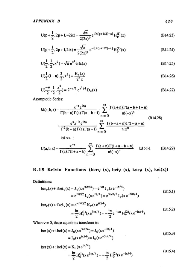
![SPECIAL FUNCTIONS 621
Differential Equations:
(1) x2y"+xy’-(ix 2 +v2)y =
Yl = herr(x) + i beiv(X
)
Y2= kerr(X) + i keiv(X
)
(2)
or Yl = ber-v(x)+ibei-v(x)
or Y2= ker-v (x) + i kei_
v(x
x4y
(iv) + 2x3y"- (1 + 2v
2 )(x2y" - xy’) + (v4 - 4v
2 + x4 ) y =
Yl = berv(x) Y2 = beiv(x) Y3 = kerv(X)
Yl = ber-v(X) Y2 =bei-v(X) Y3= ker-v(X)
Recurrence Formulae:
=-v’~(z
v-wv)
Zv+1 + Zv_
1 .
x
¯ 1
Zv = 2--~(Zv+I -- Zv_1 + Wv+
1 -- Wv_l)
v 1
= +
x
v 1
= ---z v - (Zv_1 + Wv_l)
x
wherethe pair of functions zv and w
v are, respectively:
Zv,W
v =berv(x),beiv(X) or =kerv(x),keiv(X)
or = beiv(X),-berv(X ) or = keiv(X),-kerv(x)
Special relationships
2
ber_v(x) =cos(v~)berv(x) + sin(w)beiv(x) + -- sin(v~)
bei_
v (x) = - sin(v~)ber
v (x) +cos (vr~)bei
v (x) +--2 sin(v~)kei
v (x)
Y4=keiv (x)
Y4 =kei_v(x)
ker_v(x) =cos(yr,) kerv(x) - sin(vg)keiv
kei_v (x) = sin(v~) v (x)+ cos(wx)kei
v (x)
Series Representation:
berv(X)=~- co s[r~/4(3v+2m)]
m!F(v+ ra + 1)
m=0
X
V
~
beiv(X)=~- si n[r~/4(3v+2m)]
m! F(v + m+ 1)
m=0
(B15.5)
(m5.6)
(B15.7)
fins.8)
(B15.9)
(B15.10)
(B15.11)
(B15.12)
(B15.13)
(B15.14)
(B15.15)
(B15.16)
(B15.17)
(B15.18)](https://image.slidesharecdn.com/advancedmathematicalmethodsinscienceandengineering-hayek-230318001731-2b30ece5/85/advanced-mathematical-methods-in-science-and-engineering-hayek-pdf-627-638.jpg)
![APPENDIX B 622
xn 2 x2m
kern (x) =
g(m+ l) ÷ g(n + m+
m!(n + m)!
cos[r~/ 4 (3n+2m)]-~-ffl--
m=0
2n_1 n- 1
+~ E (n-m-1)!c°s[rc/4(3n+2m)]X4--~
x
n m!
m=O
+log(2/ x) bern (x) + ~ bein (x)
X
n
kein(X)=2-’h’~" g( m+l)tg(n+m+l)sin[x/4(3n+2m)]X2S
m!(n + m)! 4’"
m=O
2n_1 n-1 x2
m
xn E (n-m-1 t
-~ m! )" sin[x / 4 (3n + 2m)]-~--
m=O
+ log(2/ x) bein (x) - ~ bern (x)
~ (-1) TM X
4m
bet(x) = m~=
0 [(2m)!]2 m
m= 0 [(2m + 1)!]
2
~ (-1) m X
4m
ker(x) = ~ 1 [(2m)!]2 24mg(2m)+ [log(2 / x) - ~) bet(x) + ~
kei(x) = (- 1)m x4 m+2
m= 1 [(2m + 1)!] 2 24m--~g(2m
+ 1)
+[log(2/ x) - 3/) bei(x)- ~ bet
AsymptoticSeries:
eX/4~
berv(x)= 2--~xx {zv(x)cosa+wv(x)sinct}
- ~ {sin (2vr0kerv(x) +cos (2vn)keiv
be
eX/4~
iv(X)= 2--~xx {Zv(X)cosa-wv(x)sina}
+~ {cos(2vn)kerv(x) - sin (2vr0keiv
(B15.19)
(B15.20)
(B15.21)
(B 15.22)
(B15.23)
(B15.24)
(B15.25)
(B15.26)](https://image.slidesharecdn.com/advancedmathematicalmethodsinscienceandengineering-hayek-230318001731-2b30ece5/85/advanced-mathematical-methods-in-science-and-engineering-hayek-pdf-628-638.jpg)
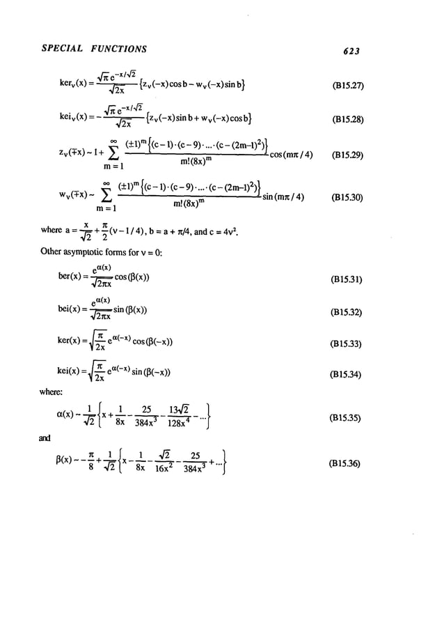
![APPENDIX C
ORTHOGONAL COORDINATE SYSTEMS
C. 1 Introduction
Thisappendix
deals withsome
of the widelyusedcoordinatesystems.It contains
expressions
for elementary
length,area andvolume,
gradient,divergence,
curl, andthe
Laplacian
operatorin generalized
orthogonal
coordinate
systems.
C.2 Generalized Orthogonal Coordinate Systems
Consider
anorthogonal
generalized
coordinate
(ul, u2, u3), suchthat anelementary
measure
of lengthalongeachcoordinateis givenby:
ds1 = g~du
1
ds2= 4
du2
where gl 1, g22 andg33are called the metriccoefficients, expressed
by:
__
fx!
1
gii du~J +~dul ) kdu~J
(C.2)
andxi arerectangular
coordinates.
Aninfitesimaldistanceds canbeexpressed
as:
(ds)2 = gll(dul)2 + g22(du2)
2 + g33(du3)
2 (C.3)
Aninfitesimalarea dAonthe u~u
2 surfacecanbeexpressed
as:
dA= [(gll)l/2dul][(gEE)l/Edu 2] = ~ duldu
2 (C.4)
Similarly, an elementof volume
dVbecomes:
dV= ~/gl lg22g33duldu2du3
= "fff
duldu2du3
(C.5)
where:
g = gl lg22g33 (C.6)
Agradient
of scalarfunction
t~, V~b,is defined
as."
~7(~=g~ll ~’ul + g~2
2 OU
2 -r g~3
3 ~U
3
(C.7)
where
e 1, e2and~ 3 are basevectorsalongthe coordinates
u1, u2, andu3 respectively.
Thedivergence
of a vector~, V.~, canbeexpressedas:
625](https://image.slidesharecdn.com/advancedmathematicalmethodsinscienceandengineering-hayek-230318001731-2b30ece5/85/advanced-mathematical-methods-in-science-and-engineering-hayek-pdf-630-638.jpg)
![APPENDIX C 62 6
V"~ = "~’{ ~ul [~f~ / gll Eli
whereE
l, E
2 and E
3 are the components
of the vector ~, i.e.:
~=EI~ ! +E2~2+ E3~
3
Thecurl of a vector ~, Vx ~ is defined as:
g~11~lr 0" ~/’~--r: 1 ~-~[ g~E2]
}
Vx~ =
TheLaplacianof a scalar function ~, ~72 ~b, canbe written as
~e ~placi~ of a vector function ~, denot~ as V 2 ~ C~ ~ written
where:
A 1 ~
0 g-~-3 E3)}: V.
~
(c.8)
(c.9)
(C.lO)
(CAD
(C.12)](https://image.slidesharecdn.com/advancedmathematicalmethodsinscienceandengineering-hayek-230318001731-2b30ece5/85/advanced-mathematical-methods-in-science-and-engineering-hayek-pdf-631-638.jpg)
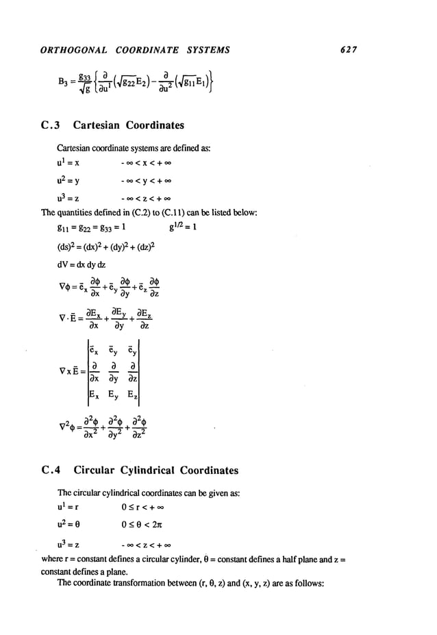
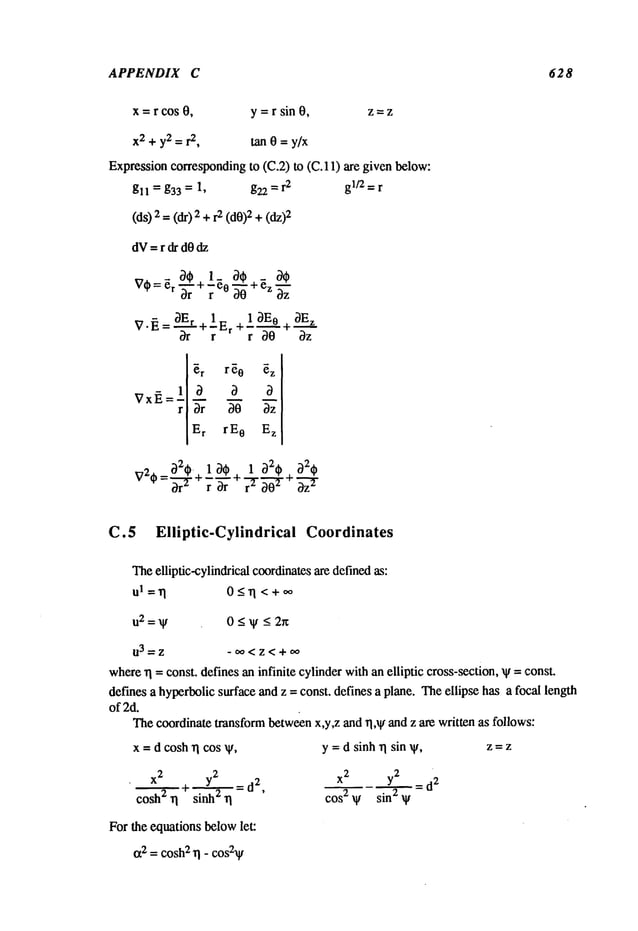
![ORTHOGONAL COORDINATE SYSTEMS 629
The quantities givenin (C.2) to (C.I 1) are definedas follows:
gll = g22 = d2 ¢x2, g33 = 1 glt2 = d2 ~2
dV
=d~
c~
daa
dV
dz
(ds)2
=#or2[(~)2+(dV)2]
+
~ ~t~v ~z/d
c~En ere v Ez/d
V2-- _ 1 ~ ~2~ a2~ 1 a2~
oz=
C.6 Spherical Coordinates
Thespherical coordinatesare defined as follows:
ul=r 0<r<oo
112--0 0<0__.~
Thecoordinate transformationbetween(x,y,z) and (r, 0, ~) are given below.
x =r sin 0 cos ~ y =r sin 0 sin t~ z = r cos 0
x2 + y2 + z2 = r
2
z ~an 0 = (x 2 + y2)1/2 tan t~ = y/x
Thequantities defined in (C.2) to (C.11) are given below:
gl ~ = 1, g22 = r2, g33 = r2 sin20 gl/2 = r2 sin 0
(ds) 2 =(dr) 2 2 (d0
)2 + r2 sin20 (d~
)2
dV= r2 sin 0 dr dOd~
V~=~ri~hlt+l_ 0~I/+ 1 - ~V
s-g’noe,"g](https://image.slidesharecdn.com/advancedmathematicalmethodsinscienceandengineering-hayek-230318001731-2b30ece5/85/advanced-mathematical-methods-in-science-and-engineering-hayek-pdf-634-638.jpg)
![APPENDIX C 63 0
OEr 2_ 1 3E o cot0_ 1 OE~
V’~’:-~’-+~’~r +~’-~’-+~ "-t~°-~ rsin0 /~
r2 sin0
~r r ~0 r sin0 ~¢
~r ~0 ~¢
E
r rE
o rsin0E¢
V2_.. ~2~ 2 3~
~ =--~- + +
cot 0 ~F 1 32~
1 ~2~/+ ~
r2 ~02 r 2 O0 ~- r 2 sin 2 0 002
C.7 Prolate Spheroidal Coordinates
C.7.1 Prolate Spheroidal Coordinates - I
Theprolate spheroidal coordinatesare defined by
ul=rl 0_<~l <~
u2=O 0<0<~
u3=¢ 0<¢_<2r~
whererI = const, defines a rotational elliptical surface, aboutthe z axis, 0 = const, defines
a rotational hyperbolicsurface aboutthe z axis and ¢ = const, defines a half plane. The
focal lengthof the ellipse =2d.
Thecoordinate transformation between(x,y~) and (~, 0, 0) are given below:
x = d sinh ~ sin 0 cos ¢,
x2 + y2 z
2
sinh2~1l- cosh2-~--
~ =d
2
,
For the equations belowlet:
IX2= sinh2~1+sin20,
y = d sinh rI sin 0 sin ¢, z = d cosh~1cos 0
Z2 (x 2 + y2) = d
2,
tart ¢ = y/x
cos 2 0 sin 2 0
and 13=sinhrl sin 0
Thequantities defined in (C.2) to (C.11) are enumerated
below:
gl I = g22=d2tx2, g33=d2[
32
glt’2 =d
3 tx2~
(ds) 2 =2 tx2 [(dl, i) 2+(dO)2] +
2 ~2(dO
)2
dV= d3 or2 ~ dq dOde](https://image.slidesharecdn.com/advancedmathematicalmethodsinscienceandengineering-hayek-230318001731-2b30ece5/85/advanced-mathematical-methods-in-science-and-engineering-hayek-pdf-635-638.jpg)
![ORTHOGONAL COORDINATE SYSTEMS 631
1
~xEn txE~
V~2 1 f~)2~ _ ¢~qt c~2V 1
V: ~ ~. ~-~-~ + c°tn ~ ~" + 3-’~" + c°t 0"~0 } + d2132
C.7.2 Prolate Spheroidal Coordinates - II
Theseare definedas
ul=~ 1_<~<~
u2=1] -1<1]<+1
u3=¢ 0_<¢<2~
Thecoordinatetransformationbetween(x, y, z) and(~, 1], ¢) are describedbelow:
x = d4(~
2 - 1)(1 - 112)COS
x
2+y2
--~z
2
x
2+y2
--=z2 d
2
1_~2 ~’~z
=d2’
~112
1 ~- 112
’
Thefocal lengthof the ellipse is 2d.
For the equations belowlet:
Ct2 = ~2 _ 1, ~2 = 1 - ~2 ~ ~2 = ~2. ~2
~e qu~fifies defin~ in (C.2) to (C.11) ~e enumerat~~low:
gll=(dx/~)2 g22=(dz /~)2, g33=(d~)2
gl~ = d3 Z2
~2 2~(d~) 2 (d~)
2
-
(ds) 2 = ~ ~ [~ + ~J + dE~E~2(d~)
2
dV= d3 Z2d~ d~ d~
y = d4(~2 - 1)(1-1] 2) sin ,, z=d~1]
tan¢=y/x](https://image.slidesharecdn.com/advancedmathematicalmethodsinscienceandengineering-hayek-230318001731-2b30ece5/85/advanced-mathematical-methods-in-science-and-engineering-hayek-pdf-636-638.jpg)
![APPENDIX C 632
V" ~ = ~X2{~[Z~z E~] + ~~ [Z~3 E~]~ ~-~ ~ }
ZE~ --~E
C.8 Oblate Spheroidal Coordinates
C.8.1 Oblate Spheroidal Coordinates - I
Theoblate spheroidalcoordinates are definedby
0<~1<~
u2=0 0_<0<n
u3=0 0<~<2~
where/q
= const, definesa rotational elliptical surface aboutthe z-axis, 0 = const, define a
rotational hyperbolaaboutthe z-axis and qb= const, is a half plane. Thefocal distance of
the ellipse =2d.
Thecoordinatetransformationbetween(x, y, z) and(rl, 0, ~) are as follows:
x = d coshrl sin 0 cos O, Y= d cosh/q sin 0 sin O, z = d sinh/q cos 0
x2 + y2 z
2 x
2 z
2
__ + __ _ d
2 + y2
= d
2 tan (~ = y/x
cosh2 r I sinh 2 ~] - ’ sin2 0 cos2 0 ’
For the equations belowlet:
c~2= cosh2
~1- sin20, and lB=coshrl sin 0
Thequantities defined in (C.2) to (C. 11) are enumerated
below:
gll = g22 = d2cz2, g33 = d2 [~2
gl/2=d
3 cz2[~
(ds)2 =2 (z2 [(d/q) 2+(d0)2] +2 ~2(d~
))2](https://image.slidesharecdn.com/advancedmathematicalmethodsinscienceandengineering-hayek-230318001731-2b30ece5/85/advanced-mathematical-methods-in-science-and-engineering-hayek-pdf-637-638.jpg)
![ORTHOGONAL COORDINATE SYSTEMS 633
1
c~ n a~0
c,En c~E
o
0211/ 0/I/ 0211/. 0~1"} + 1 021,1I
V211/=d-@~
20--@’+tanh11-ff~’~ +O-ff~-+c°sO~- d2~2 002
C.8.2 Oblate Spheroidal Coordinates - II
Thesecoordinatesare definedby:
ul=~ 1_<~<~
U2=TI -l<rl<+l
u3=~ 0_<~_<2rt
Thecoordinatetransformationbetween
(x, y, z) and (~, 11, @)are describedbelow:
X=d~/(~
2 +1)(1 - 2) co
s ~,
x2 + y2 z
2
~-d
2,
i+{2 ~ g2 -
Thefocal length of the ellipse is 2d.
For the equationsbelowlet:
~2 = ~2 + 1, 132= 1 - lq
2
y=daf~:/+l)(1-rl 2) sin~, z=d~rl
x2+y2 z2 =d
2,
tan~=y/x
1 - ~12 112
arid ~2=~2_ 112
Thequantities defined in (C.2) to (C.11) are enumerated
below:
gll=(d)~/002 g22=(dx /13)
2, g33=(dc~13)
2
gl/2 = d3 Z2
d 2
(ds)2=
2.~;t(x---~2r (d
a + 0~
@]
+ dec
~2
132 (d~)2](https://image.slidesharecdn.com/advancedmathematicalmethodsinscienceandengineering-hayek-230318001731-2b30ece5/85/advanced-mathematical-methods-in-science-and-engineering-hayek-pdf-638-638.jpg)
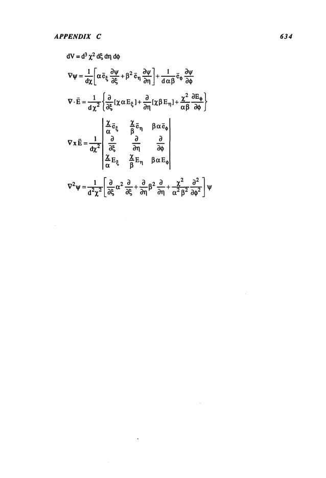
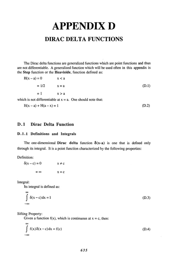
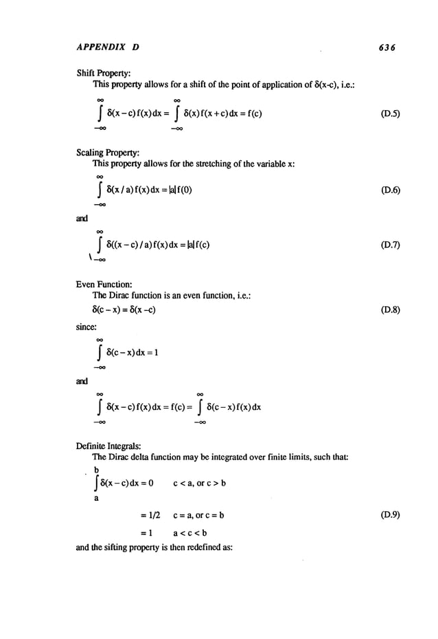
![DIRAC DELTA FUNCTIONS 63 7
b
f f(x)~i(x- c)dx c < a, or c >
0 b
a
-- 1/2f(c) c =a, or c = b - (D.10)
=f(c) a < c < b
If the integral is an indefinite integral, the integral of the Diracdella functionis a
Heavisidefunction:
X
~8(x
-c)dx = H(x-c) (D.11)
X
J
’8(x- c) f(x) dx = f(c) H(x- (D.12)
D.1.2 Integral Representations
Onecan define continuous, differentiable functions whichbehaveas a Dirac delta
function whencertain parametersvanish, i.e. let:
Limu(~x,x) = 8(x)
¢X--~0
iff it satisfies the integral andsifting propertiesabove.
To construct such representations, one maystart with improper integrals whose
values are unity, i.e. let U(x)be a continuousevenfunction whoseintegral is:
~U(x)dx (D.13)
1
then a function representationof the Diracdelta functionwhen(z --> 0 is:
u((z,x) =U(x/c0 (D.14)
whichalso satisfies the sifting propertyin the limit as (~ --> 0.
Example D.1
Thefunction u(c~,x) =(z/[rc(x2 + c~2)]behaveslike ~i(x), since:
Lim
u(0~,x) ._) {0oo
x#0
~t-->0 x = 0
andsinceit satisfies the integral andsifting properties:
X
~u((z,x)dx = 1+ larctan](https://image.slidesharecdn.com/advancedmathematicalmethodsinscienceandengineering-hayek-230318001731-2b30ece5/85/advanced-mathematical-methods-in-science-and-engineering-hayek-pdf-642-638.jpg)
![DIRAC DELTA FUNCTIONS 639
Lim(~T f(-x)
--~f(0-)
~-~0~
n ; x~--~’~-’~’~
so that, since f(x) is continuousat x =
Lim( T f(x)u(~t,x)dx --~
D.1.3 Transformation Property
Onecan represent a finite numberof Dirac delta functions by one whoseargumentis
a function. Consider8If(x)] wheref(x) has a non-repeatednull 0 and whos
e derivative
does not vanish at x0, then one can showthat:
8If(x)] ~i(x - x0 (D.15)
]f’(xo)
[
Onecan showthat (D.15) is correct by satisfying the conditions on integrability and
the sifting property. Starting withthe integral of ~[f(x)]:
I8[f(x)]dx
Letting:
U=f(x)
then:
u = 0 = f(x0) and
then the integral becomes:
j" 8[f(x)]dx-
du= f’(x)dx
]f’(xo) I I ~(x- xo)dx
I 8[f(x)lF(x)dx= I 8(u) F(x(u))du
/f’(x(u))/
_ F(x0)
[f’(xo)[ = [f’(x0)-’-~~ I F(x)8(x-x0)dx
Thus,the twopropertiesare satisfied if eq. (D. 15) represents8[f(x)].
If f(x) has a finite or an infinite number
of non-repeated
zeroes, i.e.:
f(x
n)=0 n =1, 2, 3 .... N
then:](https://image.slidesharecdn.com/advancedmathematicalmethodsinscienceandengineering-hayek-230318001731-2b30ece5/85/advanced-mathematical-methods-in-science-and-engineering-hayek-pdf-644-638.jpg)
![APPENDIX D
N
8(x- x~)
6[fix)]= E If’(Xn)
I
n=l
Example D.2
8(x2 - a2) = ~a [8(x - a) + 6(x +
oo
8[cosx]= E 8[x-2n+ln]
2
640
(D.16)
D.1.4 Concentrated Field Representations
The Dirac delta function is often used to represent concentrated fields such as
concentrated forces and monopoles. For example, a concentrated force (monopolepoint
source) located a x0 of magnitudeP0 can be represented by P0 6 (x-x0). This property
can be utilized in integrals of distributed fields whereone component
of the integrand
behaves like a Dirac delta function whena parameter in the integrand is taken to some
limit.
Example D.3
Thefollowing integral, whichis known
to have an exact value, can be approximately
evaluatedfor smallvalues of its parameterc:
T=--I
f cos(ax)Jo(bx) =1
1
7~ x2 + C2 dxc e-aCI0(bc) ~ -c
c << 1
If the integral can not be evaluated in a closed form and one wouldlike to evaluate
this integral for smallvaluesof c, onenotices that the function in example
D. 1.,
c / [n(x2 + c2)], behavesas 6(x) in the limit of c---~ Thus, one can approximately
evaluate the integral by the sifting properties. Letting:
F(x) 1 cos (a x) Jo(bx
c
then the sifting property gives F(0) = 1/c. To check the numerical value of this
approximation,one can evaluate it exactly, so that for a = b =1 one obtains:
c T(exact) T(approx) c~(exact) cT(approx)
0.2 4.13459 5.000 0.82692 1.0
0.1 9.07090 10.00 0.90709 1.0
0.01 99.0050 100.00 0.99005 1.0
This exampleshowsthat for c = 0.1 the error is within 10 percent of its exact value.
This approximatemethod
of evaluating integrals whenpart of the integrand behaveslike a](https://image.slidesharecdn.com/advancedmathematicalmethodsinscienceandengineering-hayek-230318001731-2b30ece5/85/advanced-mathematical-methods-in-science-and-engineering-hayek-pdf-645-638.jpg)
![DIRAC DELTA FUNCTIONS 643
D.5 Dirac Delta Functions in n-Dimensional Space
Asimilar representation of Dirac delta function exists in multi-dimensional space.
Let x be a position vector in n-dimensionalspace:
x = Ix 1, x2 ..... xn] (D.27)
and let the symbol
Rnto represent the volume
integral in that space, i.e.
~ F(x)dx~ ~ ~...j" F(Xl,X 2 .... xn)dXll:Lx2...dx
n
R
n -~’-~
D.5.1 Definitions and Integrals
TheDirac delta function has the followingproperties that mirror those in one-
dimensional,so that:
~(X- ~) = 1- El , x2 " ~2 ... .. Xn" ~n] (19.29)
Integral:
Theintegral of Diracdelta functionoverthe entire spaceis unity, i.e.
~ (x-~)~=l
R
n
Sifting Property:
S F(x)~5(x - ~)dx=
R
n
(D.30)
(D.31)
Scaling Property:
For a common
scaling factor a of all the coordinates Xl, x2 .... xn:
~ F(x)~5(X)dx =
[a[
n
a
R
n
(D.32)
Integral Representation:
Let U(x) = U(x
1, x2 ..... Xn)be a non-negativelocally integrable function, such
that:
fU(x)dx= (D.33)
Rn
Define:
u(~,x) = -n U(
x/a) = a-n U(
Xl/a
’ x2/~t .. ..
xn/cx) (I).34)
then:](https://image.slidesharecdn.com/advancedmathematicalmethodsinscienceandengineering-hayek-230318001731-2b30ece5/85/advanced-mathematical-methods-in-science-and-engineering-hayek-pdf-648-638.jpg)
![APPENDIX D 644
Limu(r~,x) = 8(x) (D.35)
~t-~0
This can be easily proven.through the scaling property:
Lim f -~-1 u(X)dx=f U(y)dy=l
¢t-~0 ot
n
Rn Rn
wherethe scaling transformationy = x/a wasused. It also satisfies the sifting property,
since:
f ~1 u(X) F(x) dx = Limf U(y) F(ety) dy
Lim
Rn Rn
D.5.2 Representation by Products of Dirac Delta Functions
Onecan showthat the Dirac delta function in n-dimensionalspace can be written in
terms of a productof one-dimensional
ones, i.e.:
~(X-~) = 8(X
1- El) ~(x2"~2) "’" ~(Xn" (D.36)
This equivalencecan be shownthroughthe volumeintegral and sifting property:
~ ~(x-~)dx: ~ ~(Xl-~l)dXl..... ~ 8(Xn-~n)dx
n=l
R
n -~ -~
~ F(x)~(x-~)dx=F(~)= ~ ... 1 ..... Xn)~(Xl-~l)....’~(Xn-~n)dXl...dx
n
R
n
-oo
D.5.3 Dirac Delta Function in Linear Transformation
TheDirac delta function can be expressed in terms of newcoordinates undergoing
linear transformations. Let the real variables Ul, u2 .... Unbe def’medin a single-vlaued
transformationdefined by:
U
1 =U
1 (Xl,X
2 .... Xn),2 =
U
2(Xl,X2 ... X
n) .... U
n =an (Xl,X
2 .... x
n)
then:
1
~(x- ~) =~- ~5[u- (D.37)
where~1 = u (~) and the Jacobian J is given
J(~) = det [~xi/~uj] for J(~) ~:0](https://image.slidesharecdn.com/advancedmathematicalmethodsinscienceandengineering-hayek-230318001731-2b30ece5/85/advanced-mathematical-methods-in-science-and-engineering-hayek-pdf-649-638.jpg)
![APPENDIX D 646
f 1
(D.41)
r 2 U(r)dr
0
In two-dimensionalspace:
$2(1
) = 2~t
so that the representationof the function U(r) mustsatisfy:
f 1
(D.42)
r U(r) dr = 2-~
0
Onceone finds a function U(r) whoseintegral satisfies eq. (D.38), one can then obtain
Dirac delta function representationas follows:
u(~,r) =-n U(
r/~) (D.43)
so that the spherically symmetric
Diracdelta function ~i given by:
~(x) = Limu(ct,r)
Example D.4
To construct a representation of a spherically symmetricrepresentation of a Dirac
delta function in 3 dimensionalspace fromthe function:
-r
e
U(r) =
8~t
Since:
1
fr2 U(r)dr
4--~
0
then U(r) is a Diracdelta representationin three dimensionalspace, and
1 e
-r /ct
u(~’r) = t~3
so that the spherical Diracdelta function representationin three dimensionalspaceis:
e-r/et
~(x) = ~1 Lim
8~ ct--~0 ~3
D.7 Dirac Delta Function of Order N in n-Dimensional Space
Diracdelta functionsof higherorder than zero are definedin termsof derivatives of
the Dirac delta functions as wasdonein one-dimensionalspace. Define an integer vector
l in a n-dimensionalspace as:
l =[/1, 12.... /n] (D.44)
wherel 1, l 2, ¯ ¯ ¯, l n are zero or positive integers, so that the measure
of the vector](https://image.slidesharecdn.com/advancedmathematicalmethodsinscienceandengineering-hayek-230318001731-2b30ece5/85/advanced-mathematical-methods-in-science-and-engineering-hayek-pdf-651-638.jpg)
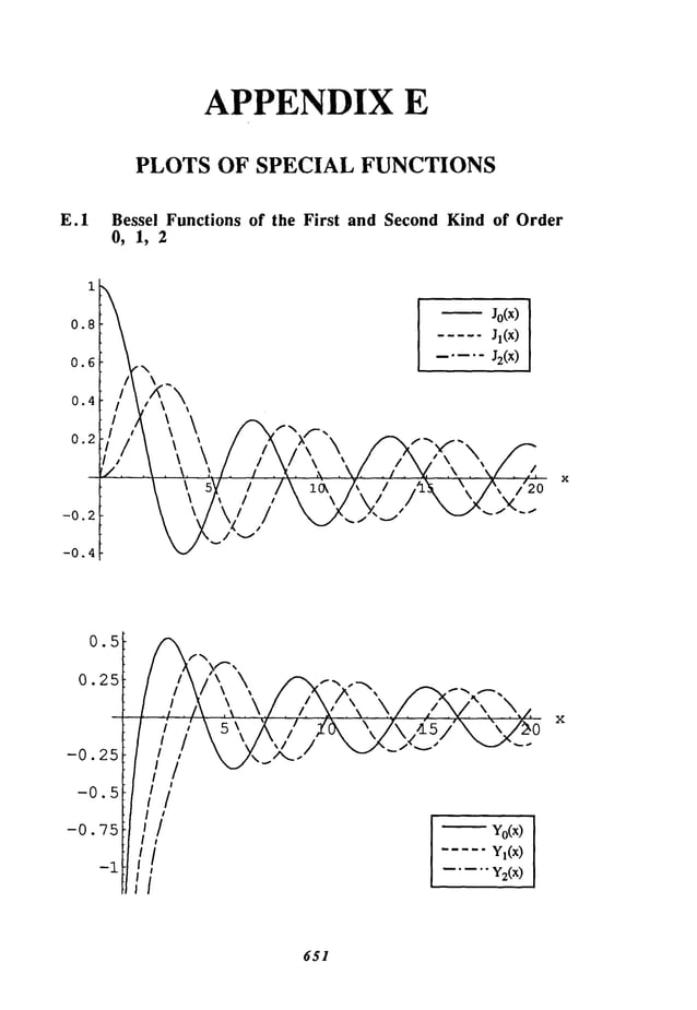
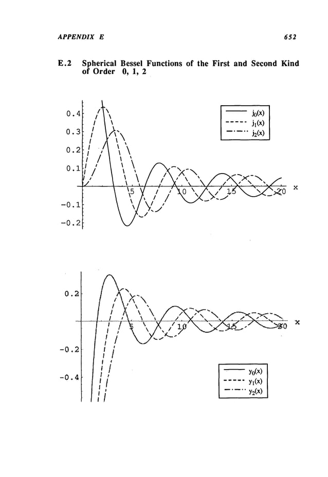
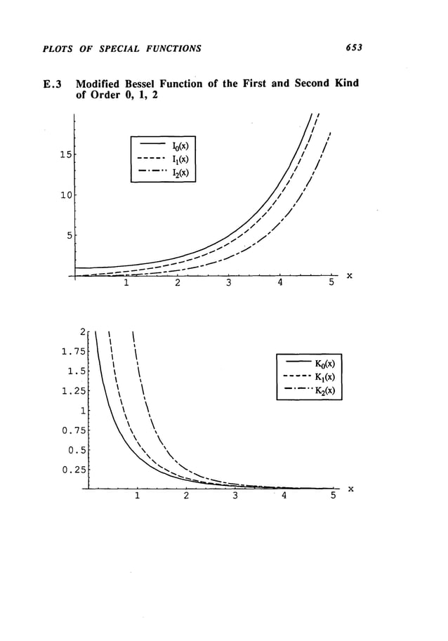
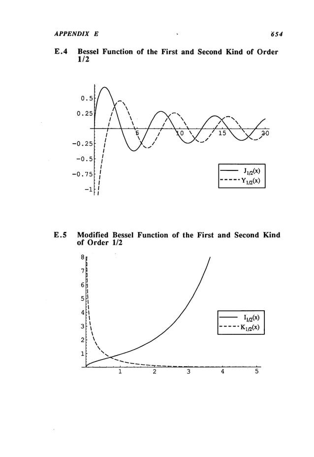
![o
ANSWERS
Chapter 1
(a) y = (c+x)e
-x~/2
CO)
y --- Cx-2+ x2/4
(C) y =C(sin "2 + (sin x)
(d) y=~l (c+lle2X+x])
cosh x ~, 21_ 2
(e) y = c cot x + csc
(f) y=ce-X+xe
-x
(a) y = 1 e-x +c2
e2x
Co)y = 1 ex/~ +c2ex/2 + c3 ex
(c) --- (ci + czx) ex+ c3 e2x
(d) y =(cl + ) e-2x + (3 + c4x)e2x
= E1sinh (2x) + E2cosh(2x) + x (E3 sinh (2x) 4 cosh (2x))
(e) y = 1 e2x+c2e-2x + c3 e2ix + c4 e-2ix
= E
l sinh (2x) +2 cosh (2x) +
3 sin(2x)+ ~4co
s (
~2
i
,-l+i ,
(f) y = clexp( x) + c2 expt--~-x)
(g) y ="z (I sin z +c2cos
z) +z (3 sinz + c4 cosz)
= E1sin z sinhz +E2sin z coshz + ~3cos z sinhz +~4cosz coshz
where z =
(h) y=e
x(c
1+c2x+c3
xz)+ e-x(c
4+c5X)
(i) y = e-2ax+ eaX[.c2 sin(ax~/~) +3 cos(ax~/’~)]
O)Y= cl e’aX+ eax [ c2 sin (ax) + 3 cos (ax)]
(k) y = 1 +c2x) sin (ax) + 3 + Ca
X
)cos (ax)
(I) y = Cl sin (2x)2 cos
(2x)+ e-x~f~ (c3 sin x+ c4co
s x)
+ ex4~(c5 sin x +c6 cos x)
663](https://image.slidesharecdn.com/advancedmathematicalmethodsinscienceandengineering-hayek-230318001731-2b30ece5/85/advanced-mathematical-methods-in-science-and-engineering-hayek-pdf-666-638.jpg)
![ANSWERS - CHAPTER I 664
o
o
(a) = ClX + C2
x-I
(b) y = ClX-1+ c2x-1log
(e) y = e! sin (log 2) +c2cos(log2)
(d) y = ClX+ x’l + c3x2
(e) y = (c~ 2 logx) x+ c3x-2
(f) y = ClX+ c2x-2+ 3 sin ( log x2) +c4cos(log2)
(g) y = 1/2 (I + c2logx)
(h) y =1/2 [c1 sin (log x) +2 cos
(logx)]
(a) yp -- -2ex - 3 sin x +cos x - (3x2/2+ x) "x
Co)yp = 2 -3x+ 9/2+ e-x + (3x4/4 - x 3+ x2)ex
(c) yp= [sin (2x) 2 sinh (2x)]/4
(d) yp = 2 +2xlogx
(e) yp = 2 +2x
(log x)2
(a)
(b)
(c)
(d)
x
y =c1 sin (kx) + 2 cos(kx) +
~ ~ sin (k(x - rl )f(rl)drl
1
x
y=clx +C2
x-1 + ½j" (xrl-2 - x-l) f(~)drl
1
x
y= ClX + C2x2 +C3X2 logx+ ~(xrl-x2(l+ log rl)+x 2 log x) ~d~l
1
x
y = Cl
ekx+c~e
-kx+ k
1- ~ sinh(k(x - rl)f(rl)
1](https://image.slidesharecdn.com/advancedmathematicalmethodsinscienceandengineering-hayek-230318001731-2b30ece5/85/advanced-mathematical-methods-in-science-and-engineering-hayek-pdf-667-638.jpg)
![ANSWERS - CHAPTER 2 665
Chapter 2
(a) p ---> 0%oo<x<.o
(b) p-~,,,,, - .o<x<,,*
(c) p=l, -l<x<+l
(d) p=l,-l<x<l
(e) p=l, -l<x<l
(f) p =2, -2<x<2
(g) p=2, -2<x<2
(h) p=4, -4<x<4
(i) p=2, -l<x<3
(j) p=3, -4<x<2
x 3 x
6 x 4 5x
7
(a) y =Cl[1-’~’+~-"’]+c2[x-’~-+45 ~- "’’]
(b) y=cl[l+
x 2 x 4 1.3x
6 1.3.5x
8
¯
I +...] +¢2
x
21! 222! 233! 244.
t
0o x2
m
(C) y=c 1 Z
2ram!
m=O
x3 x5 x
7
~ + C2[X + ~ + ~ + ~ + ...]
3 3"5 3"5"7
(d) y = CI[I+x 2 +11X4+ZX
6 +...]+C2[X + 7. 3 +2X
5 +5X7+...]
12 12 4 12
x 3 x 4 llx 5 13x 6 . . x 3 X4 x 5 x
6
(e) Y=Cl[l+x2+--+m+~+~+ .l+c2tx+ + ...]
6 3 120 180 "" "~’- + "~" + "~" "~+
x3 x
6 x4 5x
7 3x 5 9x
g
(0 Y = Cl[1-’~"~ + -"r~---...]+C2[X--m+~--...]+C3[X
2-~+~-
645 6 252 20 560
.o.]
(g) Y=Cl Z (-1)n(2n+l)x2n+c2 (-1)n(n+l)xZn+t
n=O n=O
~
X2
n
(h) y = Cl(X-X3)+c2
(2n- 3)(2n-
n=O
x2 x3 3x 4 . . x 2 2x
3
(i) Y=Cl[l+~+--+~+ l+c2x[l+~+~+...]
2! 3! 4! "’" 3[ 4!
oo
x4n+
2
00
X4
n
(J) Y=Cl Z (-l)n(2n+l)[
~-c2 Z (-l)n
(2n)!
n=O n=O](https://image.slidesharecdn.com/advancedmathematicalmethodsinscienceandengineering-hayek-230318001731-2b30ece5/85/advanced-mathematical-methods-in-science-and-engineering-hayek-pdf-668-638.jpg)
![ANSWERS - CHAPTER 2 666
3. (a) y
(x+1)
2 (x + 1)3 5(x + 1)
4
2 3 24
+ c2 [(x + 1)- (x + 2 +
2(x + 1)3 5(x + 1)
4
3 12
(x - 1)4 (x - 1)8 (x - 1)
12
(b) Y=Cl[l+ ~ ~ +...]
12 12.56 12.56. 132
(x - 1)5 (x - 1)9 (x - I)
13
+ C2[(X -- 1) + ~ + ~ ~-...]
20 20.56 20.72.156
(c) y=c 1 E (2n+l)(x-1)2n+c2 (n+l)(x-1)2n+l
n=0 n=0
Y= Cl E (n + 1)(2n + 1)(x 2n
+ c2 E (n + 1)(2n+ 3)(x2n+1
n=O n=O
(a) x = 0 RSP
(b) x = 0 ISP
(c)x=+ 1 RSP
(d) x =0,+_ 1 RSP
(e) x=0, nnRSP n=+1,+2,+3 ....
(f) x =0ISP, x=nr~RSPn =+_ 1,+_2 ....
(g) x = 1 RSP
(h) x=0,1RSP
(a) Yl = x3/2(1-3x+1-~5 x2 - 3"-’~’5 x3 +...), Y2= x(1-x+2x2-2-x3 +...)
4 32 128 3 5
~ xn+l
00
xn_3/2
(b) y=c 1 (-1)nr(n+7/2) +c2 E (-1)n
n"--~.t
n=0 n=0
where:
l"(n + 7/2) = (n + 5/2) (n +3/2) (n + 1/2) ... (3 + 1/2) (2 +1/2) (1
oo
xn+l/2
(C) y = 1 E
(-1)n (n+ 1t + C2X-
1/2
n=0
oo xn+l
(a) y=c
I E (n+2)-’----~,
+c2[l+x-l]
n=O
(e) Y=Cl E (-1)n
x4n+
3
oo
x2n+
2
1.3.5.(2n+1) +c2 E (-1)n 2nn’--’~
".
n=0](https://image.slidesharecdn.com/advancedmathematicalmethodsinscienceandengineering-hayek-230318001731-2b30ece5/85/advanced-mathematical-methods-in-science-and-engineering-hayek-pdf-669-638.jpg)
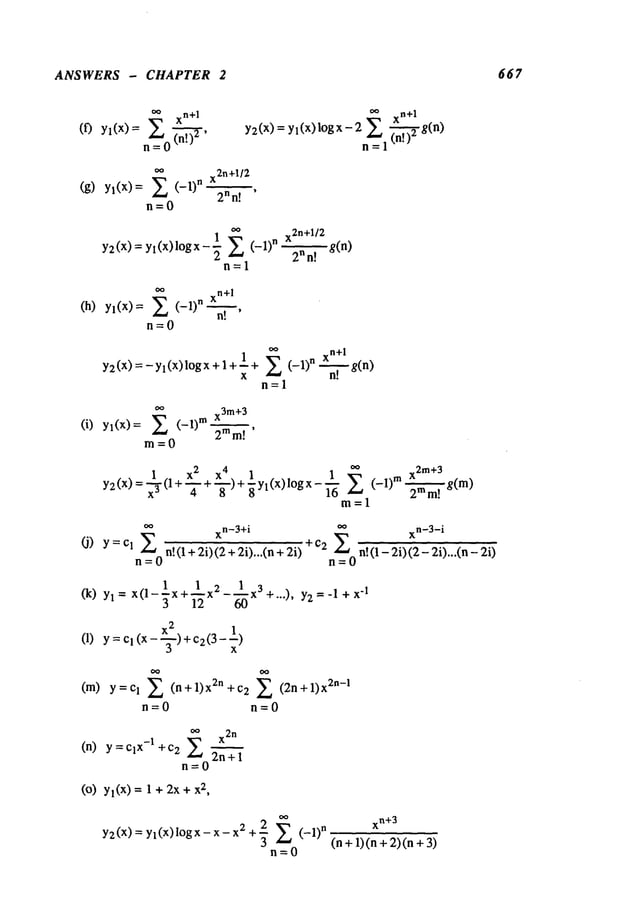
![ANSWERS - CHAPTER 2 668
,x, 2n
Yl(x)
n!)2,
oo
xn
Yl(X)= ~’~ (--1)n(n.~
~,
n=O
(r)yl(x)=
(s)
~o X2
n
Y2(x)=yl(x)l°gx- Z (~.~.,~g(n)
(0
¯ n
Y2(X)=Yl(X)logx-2 ~ n ~.~- -~-g(n)
n=l
~ (_l)n 2n
(n +1)!n!’
n=O
Y2(x)=YI(X)I°gx-x-2 l+x2- (- 1)n(n~-~[l+2ng(n-1)]
rl=2
Y=CI(I+-~x+-~-~-)+C2X4 ~_~ (n+l)x
n
n=O
oo
n x2n
Yl(x)=x Z (-1) (n!--~’
n=O
oo
X2
n
Y2(x)
= Yl(X)l°gx-
(-1)
(n!-~
g(n)
n=l "](https://image.slidesharecdn.com/advancedmathematicalmethodsinscienceandengineering-hayek-230318001731-2b30ece5/85/advanced-mathematical-methods-in-science-and-engineering-hayek-pdf-671-638.jpg)
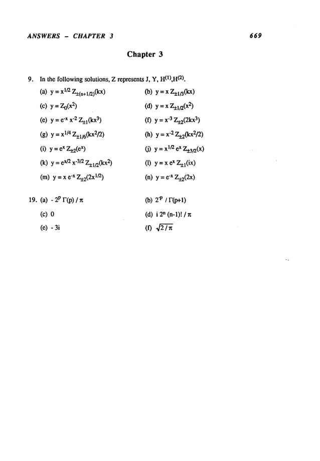
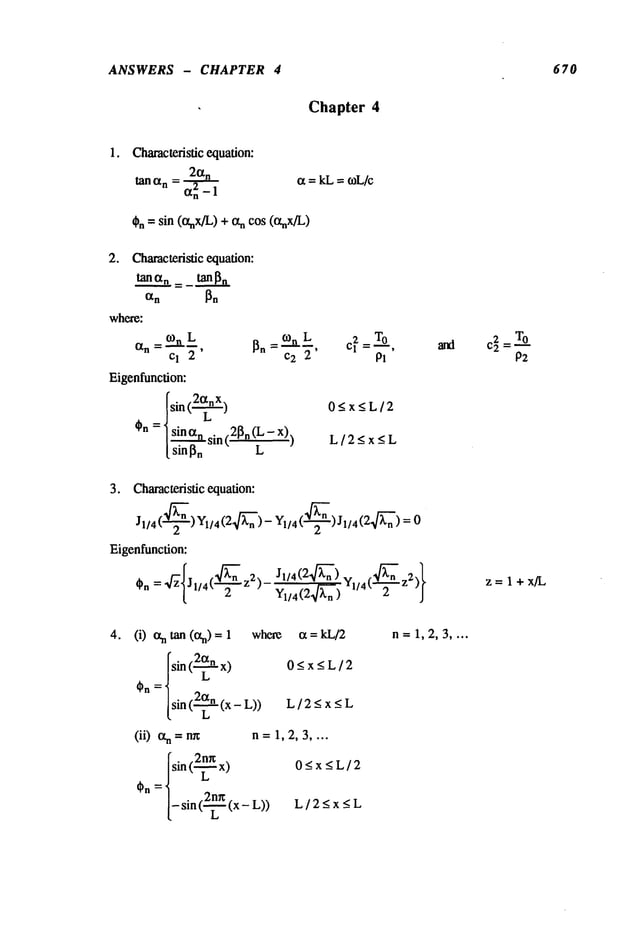
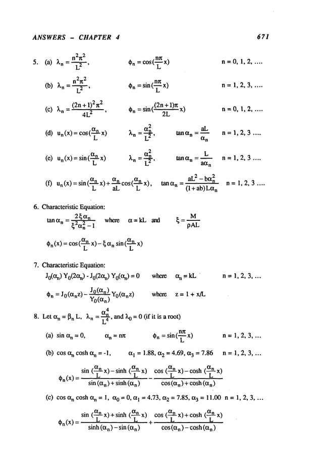
![ANSWERS - CHAPTER 4 672
(d) sin n =0,an = nx Cn = cos(--~x)
(e) tan an= tanhan, I = 3.93, 0.2 = 7.07, a3= 1
0.2
n=O,1,2 ....
n=1,2,3 ....
Cn(x)
sin (--~- x) sinh (~-
sin (an) sinh (an )
(f) tanan=tanh [see(e)l n=0,1,2 ....
(g)
Cn(X)
sin(~--~x) ÷ sinh(~--~
sin (an) sinh (a
n)
2~,L
3
cothan - cot % = ~ n= 1,2,3 ....
%(x)
sin (~- x)
sin(an)
sinh (~- x)
q-
sinh(an)
(h)tanan- tanh
an=2rl__..~L
an El
n= 1,2,3 ....
(i)
¢.(x)
sin (~-~x)a sinh (~-
cos(an) cosh(an)
3
cosh an COSan + 1 = ~ [sinh an cos{X
n - coshan sin an ]
an E1
n= 1,2,3 ....
(J)
sin (-~-~ x) - sinh (-~- x) cos (~- x)- cosh(-~-
Cn(X)
sin (an) + sinh (a
n) cos(an) + cosh(a
n)
~L
cosh an + cos an + 1 = - ~ [cosh a n sin an + sinh an cos an ]
an E1
n-- 1,2,3 ....
On(X) +
cos(an) + cosh(an ) sin (an) - sinh (a
n)
9. CharacteristicEquation:
tanh an = tan an+2k an tan antanh an
an=~n L, ~Ln =-.~-¢~,n=1,2,3 ...](https://image.slidesharecdn.com/advancedmathematicalmethodsinscienceandengineering-hayek-230318001731-2b30ece5/85/advanced-mathematical-methods-in-science-and-engineering-hayek-pdf-675-638.jpg)
![ANSWERS - CHAPTER 4 673
On(x)
sin (~- x)- sinh (-~- x) cos (~- x)- eosh
sin (an) + sinh(a
n) cos(%)+cosh(an)
10. Characteristic Equation:
(a) k an (tan %- tanh ~) where
sin (~-~- x) sinh (~-~- x)
I}n (X)= 0 < x < L/2
cos(a
n
) cosh (Ix
n)
=- sin (z) + tan n) cos (z) + sinh (z
) - tanh (an) co
sh (z
an = ~nL/2, k = M/ (pAL)
L/2<x_<L
wherez = an (2x - L)/L
(b) sin an =
2n~
Cn= sin ("7-- x)
L
0Ax~L n=1,2,3 .....
11. Characteristic equation:
Jn(13~m)In+l(13~m)+ Jn+l(O~rn) ]n(0~m) where
xn/2[ Jn (2~mL’~x’~) In (2 ~mL,~"7"~)
On = [_ Jn(2~m
L)
~
am= 2 l~t.
m=1,2,3 ....
12. (a) Characteristic Equation:
sin an,= 0, an = kn L = nn
n= 1,2,3 ....
sin (? x) n~ x)
nr~ = Jo("~"
--X
L
2
(b) tanan=a
n an=knL ~’n an n=0,1,2 ....
~o = 0, aI = = 4.49, a2 = 7.73, 0.3 =10.90
(LmXx) . nrr
sin
nn = Jo(-~-- x)
~X
L](https://image.slidesharecdn.com/advancedmathematicalmethodsinscienceandengineering-hayek-230318001731-2b30ece5/85/advanced-mathematical-methods-in-science-and-engineering-hayek-pdf-676-638.jpg)
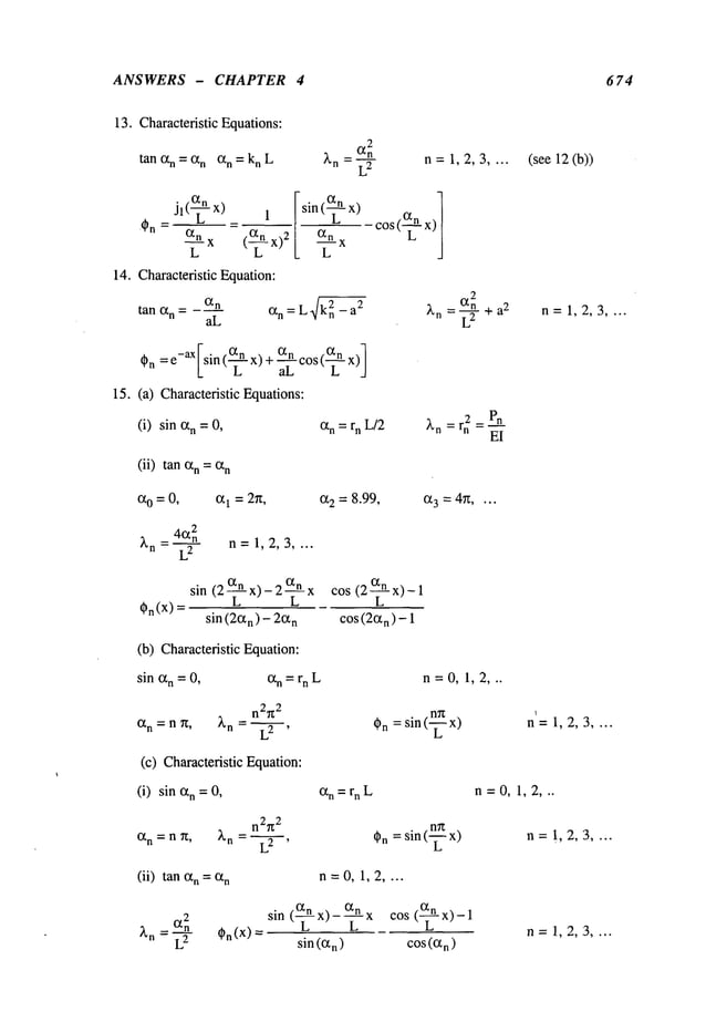
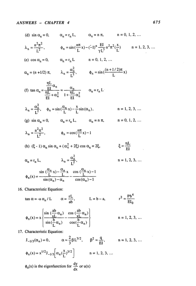
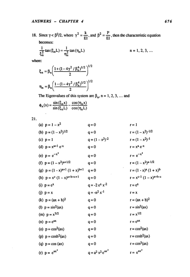
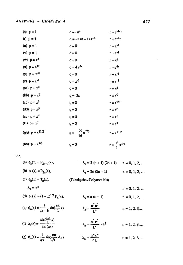
![ANSWERS - CHAPTER 4 678
(h) On(x) "a x]2 sin(~x)
sin(--~ x)
(i) On(x)= cos(ax)
sin(-~x)
(j) %(x)
=cosh(ax)
(k) On(x)=-ax’/2 sin(-~x)
e-2ax - 1
(1) On(X)= ¢ax sin (n~ ¢-2aL)
~n=[" 2nr~a
[ e_-~-~"-
1’]
2
I1~x
1-2a
(m) On(x)=s sin(, L -i~_2a )
a: r (2a - 1) n~
’~=L’L
r-~
J
(n) On(X)
= x sin (2nrt 1)
x
(0) On(x) 1/2 Jl [13tn(x/L)l]2]
n2~ 2 a
2
Ln = --~- +
~- n--: 1,2, 3 ....
n2g
2
~= L~-,F--a
2 n=1,2,3 ....
n2~
2
Xn= L--~+a2 n=1,2,3 ....
n2~
2
~ = --~-- + a n=1,2,3 ....
n= 1,2,3 ....
n=1,2,3 ....
;~n=4 n2n2 n = 1,2, 3 ....
2
Jl(an) =
X~-~-~
n =I, 2, 3 ....
¯ [sin(a n x)
]
_ " [ L
cos(an~)
(p) O.(x) ......
X2
~n ~
I,2,3,
(~%(x)
-~
sin
(nnx ~=n~=2 n=I,
2,
3....
(O%(x)
3~
J: [
~(x
~)
3~1
Jl(an) =
(s) ~n(x) = x sin (mr log
-L3
n=1,2,3 ....
~n= n2n
2 n =1, 2, 3 ....](https://image.slidesharecdn.com/advancedmathematicalmethodsinscienceandengineering-hayek-230318001731-2b30ece5/85/advanced-mathematical-methods-in-science-and-engineering-hayek-pdf-681-638.jpg)
![ANSWERS - CHAPTER 4 679
23.
sin(-~ x) n2r~2
(t) ,o(~)=~/.~.~, ~=
L..-L-.
~-
(u) On(X)
"3
sin (n~ (x/L 4)
n= 1,2,3 ....
16 n2g
2
~,n = LS n=1,2,3 ....
(V) On(X)"1J3[1 3tn(x/L)l/3]
J3(~tn) =
(w)t~n(X
) =x
-5/’2 J5/2[l~nX/L]
or
2
~-~
n=1,2,3 ....
tan (~n) 30~n
2
3-~
n
(X)¢~n(X)
-3/2 J3/4[l~nx2/L2]
J3/4(~.n) = ~’n = 4 L’~
(Y)(~n(x)=x’1/2J1/4[i3tnx2/L2
]
2
Jl/4(t3tn)= ~n = 4 L.4
(Z) ~bn(X
) = X
"9/4 J2[O~n(x/L)
3/2]
J2(ff, n)=
(aa)0n(X)
"1
/7 J1/x4[ff.nx2fl_,
2]
Jl/14(ff.n) = ~ = L4
- 1 --/-- ~COS/~
n
~bn(X)- ~/~ [~n---~x 2 sin( t~nL) CtnXk,
~ =-~-~- n=1,2,3 ....
n=1,2,3 ....
n= 1,2,3 ....
n=1,2,3 ....
n=1,2,3 ....
(a) y = An sin(--~x) An 2
n2~2 =r f f(x>sin(--~x>
dx
n=l ~.-~](https://image.slidesharecdn.com/advancedmathematicalmethodsinscienceandengineering-hayek-230318001731-2b30ece5/85/advanced-mathematical-methods-in-science-and-engineering-hayek-pdf-682-638.jpg)
![ANSWERS - CHAPTER 4 680
YI= [3 cos (kx)- 3 cot (k) sin (kx)] x,
4ex/2 ~, sin (nrc,~)
(e) y = ~ =~
,3 .. ..
n (~,- n2n
2 / 4)
,,o
sin(nnx2
)
= 4e~ ~
(0
~X
2 n
n=1,3....
4 ~ sin (nnx)
gxn =~3....
n(k~ - n~)
where L
a is the root of Jo(~/~L) = O, and
4e3X ~
~ an J2(~n
x2)
(i) y=
O)
(k) y=--
(I)
(m) y=-~
J2(otn) =
n=l
[j;(an)]_ 2 1
= ~ X2 J2(~nx2)dx
an
k- 4Ct2n 0
O0
4e
2x
~ sin (nr~x
2)
Y=~ x-"~n=:~,3, ... n (~’- 4n2n2)
00
2
4e
x
~-~.
sin (mrx)
gX7/4
n =~,3 .... n~)
2 "~ Jl/4(~n-~
"2)
ex (x]_,) 1/2 /--’
n = 1 (~,- 4-~-)~ n J~/4(~n)
oo
sin (nr~x
3)
4eX
Z n (~, - 9n2r~
2)
~x
3
n=1,3....
+1
2n+l
J f(x):Pn (x)
2
-1
4ex ** sin (mrx)
YII = "’~ Z n(l~_ n2~2)
n=1,3....
2
Jl(OCn) =0 ~n--’~"](https://image.slidesharecdn.com/advancedmathematicalmethodsinscienceandengineering-hayek-230318001731-2b30ece5/85/advanced-mathematical-methods-in-science-and-engineering-hayek-pdf-683-638.jpg)
![ANSWERS - CHAPTER 4 681
24.
25.
26.
4eX
~
sin(nr~x4)
(n) y = nx-~
~-
n(k2 _16n2n2)
n=1,3....
(a) 2r~2(-1)n+lsin(nx)8 2
n ~
n=l n=l,3....
(b) ~
m=l
(c) 2 E (-1)n÷l sin(nx)
n
n=l
8
2
sin (nnx)
(d) -~-
n3
n=1,3....
(e) ~- n’~+l
n=l
(f) sin
(a) ~-~+4~(-1)n~
n=l
1 2 E (-1)n+~ cos((2n-1)x)
<b)
n 2n-1
n=l
O0
(c) n__ 4 E cos ((2n - 1)x)
2 n (2n - 1)
2
n=l
1 1 x cos (2nx)
(d) ~-~-T E 2
n=l
en-1 2 E [1-(-1)"en]C°S~(2nx)
(e) n
n n ~ +1
n=l
2_4 cos(.__2nx_)
(0 n nn’~__l 4n2_1
1 1 . 2 ~ cos(2nx)
(a) ~-+~s~nx--~n,~,__ 1 (2~~+
(b) 2asin(an)I 1,+ ~ n cos( nx)"
sin(nx)
n
3](https://image.slidesharecdn.com/advancedmathematicalmethodsinscienceandengineering-hayek-230318001731-2b30ece5/85/advanced-mathematical-methods-in-science-and-engineering-hayek-pdf-684-638.jpg)
![ANSWERS - CHAPTER 4 682
1 4 ~_~ cos(n~x)
(c)
3 r~
2 (-1)n 2
n=l
n sin (nx)
(d) 2sin(a~)X (-1)n-~2
~g -
11=1
~+~ ~ sin(rig/2) . x. 1 co s(n~/2)-cos(n~)s~(n~
)
(e)
~ ~ n
~
,cos tn~ ~ - -
n=l n=l
2 X (-1)n sin(n~x)
n
n=l
27. f(x)=~ X
n=ll-tn[ 1( l~n)J
28. f(x)=-2n~ J2(~nX)
=1 la.
Jo(l.tn
x)
29. f(x) = 2a X2 + i. t2nL2) jo(~tnL)
n=l
30. f(x) =--+-- [P2n(0) - P2n+2
(0)] P2n+1
2 2
n=O
1 1 5
31. f(x) = ~- PO+ "~ PI(x) + ~ P2(x) + "’"](https://image.slidesharecdn.com/advancedmathematicalmethodsinscienceandengineering-hayek-230318001731-2b30ece5/85/advanced-mathematical-methods-in-science-and-engineering-hayek-pdf-685-638.jpg)
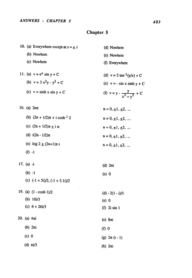
![ANSWERS CHAPTER 5 684
21.
z
2n
(a) 2 (-1)n (2n)-’-~
n=O
(b) ~ (-1)"
n=O
Z
2n
(2n
lzl
<oo
23.
24.
(c) (- 1)n(n+l)zn Izl <1
n=O
Z (-1)n~ Iz-21<2
(e)
n=0
(g) ~ (n+l)(z+l)
n Iz+ll<l
n=O
(i) 2 ~(z -2)
n Iz -21<
nt
n=O
o~ zn
(d) ~ (n + I)!
n=O
(f) -1-2Z (z-l)
n
n=l
oo
(z - 1)
n+l
~(z
- ix)
n
(J)-
n!
n=O
Iz- 11<1
Iz - 11< 2
[z - ixl <oo
~ zn-
3 ~ z-
n
(a) Z--~.~ (b) Z-~-.~
n=O n=O
(C)--ZZ-n n=~,#o2n+, (d) Z (Z--1)-n-2
n=l - n=O
(e) - (Z--1)n-1
n=O
(f) [(2i- 1)(-1) n - (2i + 1)]inz -n-! + -1 n z n
= n=O J
(g) 2 (-1)n (z- -n-2
n=O
1)
n
(h) (z+l)-n- Z
+
2n+l
n=l n=O
(a) Simplepoles:
(b) Simple pole:
(c) Simplepoles:
z= (2n+1) r~/2, n = O, T-l, g2 ....
z=O
z= -T-i~](https://image.slidesharecdn.com/advancedmathematicalmethodsinscienceandengineering-hayek-230318001731-2b30ece5/85/advanced-mathematical-methods-in-science-and-engineering-hayek-pdf-687-638.jpg)
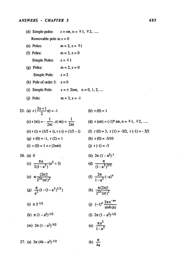
![ANSWERS - CHAPTER 5 686
(c)
(4a3)
-1 (d)
(f)
~(2a+b)
2a3b(a + b)
2
3n
O)
(n)
2ab(a + b)
2(a+b)
28. (a) 2bea
b
g -ab _ c~-ac)
(c) 2(b2 _c2)
n (1 +ab)
(e) 4 b3eab
n (e-ab _ e-aC)
(g) 2(C 2 -b
2)
(i) "ab n/2
(cos (ab) - sin (ab))e-abg"I
(b) ~ sin (ab)
(d)
2--~e~
cos
~
_ ce
-ab)
(f) 2bc(b2 - c2) (
bc-ac
(h) r~ a -ab (4b)
-1
(j) r~ (1 -ab/’2)e-ab/2
xa(l+ab)
(1) 16bSea
b
29.(a)
(c)
(c)
(g)
O)
(k)
ncos(ab)
- I/4
(12)
-v2n
.3-~/2~
- n [e"ab+ sin (ab)] / 3
(m)[e-ab - sin (ab)] rc / (4b)
(b)
(d) n [2 - c’ab(ab+ 2)]/(8b
4)
(0
(h)
(j) -~ sin (ab) /
(1) n cos (ab)
n
[c sin (ab)- b sin (ac)]
(n) 2bc 2 - b2)](https://image.slidesharecdn.com/advancedmathematicalmethodsinscienceandengineering-hayek-230318001731-2b30ece5/85/advanced-mathematical-methods-in-science-and-engineering-hayek-pdf-689-638.jpg)
![ANSWERS - CHAPTER 5 687
(O)8--~[1 - "ab cos (ab)]
(q) 2(C2_b2)[b sin (ab)-c sin
(S) ~ 2[bE sin (a b) - 2 sin(ac)
2(b -c )
(p) ~ -ab + cos (a b) -
(r) - ~ [(2 + ab)e-ab + sin (ab)]
(t) [cos (ab) "ab] n / 4
31.(a)
(c)
(e)
1
sin(at) /
t cos(at)
t
n
(g)
n!
(i) - cos (a
0c) sin (at) +at cos (at)
(m)cosh(at) - cos
(b) -bt - e-at) / (a- b
(d)cos(at)
(f) -bt sin (at) /
(h)cosh
(at)
(j) sin (aO- at cos (at)
O)sinh (at) - sin (at)
32. (a) F(x)={10 0<X<ax>a
(c) F(x) =
(b) F(x)=
a
(d) F(x) = (1 + -ax / (2a3)
38. (a) ~r3/16
(c)5/32
5
(e) - r~2,4~/16
(g)- n/2
(i) - 23~r /
(k) -r~ ~ cos(~)
4n
:~ sin2 (~n)
(m) 2 / (4a)
Co)
(d) 3
(0 - ~/4
(h) 2ab(b2_ a2) [b log a - a log
(J) 3 1+ cos2(~n)
8n
3 sin3 (~n)
r~aloga
(1) 2(1_a2
)
(n)
39. (a) rr (1 - a) / (4 cos(a~/2)) (b) - rc / sin (an)](https://image.slidesharecdn.com/advancedmathematicalmethodsinscienceandengineering-hayek-230318001731-2b30ece5/85/advanced-mathematical-methods-in-science-and-engineering-hayek-pdf-690-638.jpg)
![ANSWERS - CHAPTER 5 688
40.
(~_)arc ba _ c
a
sin
(c) 2rc~/~sin (arc) (d) rc (b- c) sin
(~) rc sin (ab)/ [sin (b) sin (0 - ~ cotan (art)
(g) a ad cosec (an) (h) (-1)nba+l-n cosec(arc) F(a + 1)
F(a- n + 2)
(i) (c +"3 rc/ 2 (j) a co
sec (an) - a cot(a~)] rc / (b +
- rc cot (ax) (ca- ba) / (c (1) ~-~ rc cosec (~)
(k)
(a)2rc,/3/(9a)
(b) rc cosec(~/5) / OR
~a (2 sin (~) + sin (a
(c) rc / (4a2) (a) n cosec(2rd5)/ (5a2)
(e) rc ~]3/ (9a) (0 n cot (rc/5) / (5a)
(g) -~ cot (2rc/5) / (5a3) (h) 1 / (2a
2)
(i) 1 / (3a3)
41. (a) (l°gb)2-(l°ga)2 0a) loga
2 (b - a) a
(c) - 2 rc2 / (d) 2 rc2 /
(e) [rc2 +(log 2] / [2(a + 1) (f) log a [rc2 +(log 2] / [3(a + 1)
(g) 2n2/3 (h) 4rc2/27
(i) 4 rc2 / (j) 2 / 27
42. (a) 1 ee.~ erf(a~]~’) (b) (nl)-1/2 - aea~t [1 - erf(a,~’)]
a
(C)(rct3)
-1/2[ebt - eat] / 2 (d)(~;t)-1/2e
-at
tb-I e-at
(e) 1 {1 - edt [1 - erf(a4~)]} (f)
a F(b)
(g) OforO<t<a, e-~(t’a) fort>a (h) (m)d/~cosh(2a,~
")
(i) (/tt3)-1/2e-a/4t a1/2/ 2 (j) "at- e"bt) ] t
(k) 2 (cos (at) - cos (bt)) (1) 2 cos(cO-bt - e-at) / t
(m)
(1+:2bO
bt(rcO
-1/z (n)(rcO
-|t2](https://image.slidesharecdn.com/advancedmathematicalmethodsinscienceandengineering-hayek-230318001731-2b30ece5/85/advanced-mathematical-methods-in-science-and-engineering-hayek-pdf-691-638.jpg)
![ANSWERS . CHAPTER 5 689
(o) Jo(at)
(cO(m/2)-~t2
cosh
(s) (log 2 -r~2 / 6
(u) 0 for 0 <t < a, Jo(bt) for t
(w)-(a+b)t Io[(a-b)t]
(y) ’f~- (~a)V
J v (at) / F(v
(aa) ea~terfc(a4~
")
(19)(~14~2)
"I/2COS(a0
(t) (cos(at) +at sin (at) - 2
ca2t
(v)--+
b+a
aea2terfc(a.~/~’)- beb~terfc
(b.~’)
b2 _ a
2
(x) t e(a+b)t[Ii[(a-b)t]+Io[(a-b)t]]
(z) v Jr(at)
Cob)
-at erf [ (Co-a)t)
1/2](b-a)
-it2
2 2
ea~t aeb terfc (b~/~) - a terfc(a.~/~)
(cc) ~
b+a b2 _ a
2
(dd)a -at [Io(at) +Ii(at)]
( a ~1/2
(ff) 4~-~t ) exp(-
(hh)sin (at)
(ee) 2 (1 - cos (at))
(gg) (m)-~/2 exp(-~tt)](https://image.slidesharecdn.com/advancedmathematicalmethodsinscienceandengineering-hayek-230318001731-2b30ece5/85/advanced-mathematical-methods-in-science-and-engineering-hayek-pdf-692-638.jpg)
![ANSWERS - CHAPTER 6 690
Chapter 6
1 - COS
T(x,y) 2TobL
n=l
wheretan ot
sinh (tzny] L) sin (~n X [ L)
sinh (~n)
Z an sin (nrcx / L) exp (-n~y /
T(x,y)-- ~
11--1
L
a
n= J f(x)
sin
(nxx
/
where
0
2To oo b2L2
+ ctn
2 cos
(¢XnX
/ L)exp
(-CtnY
/
T(x,y) = ~ Z an b2L2 +bL+a2n
rl=l
L
wherean=Jf(x)cos(~tnx/L)dx and tan ff’n = Lb/ff’n
0
o
2T
0 cosh (nny/ L) sin (nwx/ L)
T(x,y) = ~ an
cosh (nn)
n=l
L
an = J f(x) sin (nr~x/
where
0
0~ 1 (r~2n+l
5. T(r,0)= 4T°n Z ~h"~~] sin((2n + 1)O)
n=0
~ an - sin (n~0 / b)
n=1
b
where an = f f(O)sin (-~O)dO
0
T(r,O) = (an cos (nO)+n
7. sin(nO))
n=l
2x
where an = lO J f(0) cos (nO)
dO
0
2~
bn = t0 J f(0) sin(n0) dO
0](https://image.slidesharecdn.com/advancedmathematicalmethodsinscienceandengineering-hayek-230318001731-2b30ece5/85/advanced-mathematical-methods-in-science-and-engineering-hayek-pdf-693-638.jpg)
![ANSWERS - CHAPTER 6 691
9. T(r,z)=-~-- cn
n=l
sinh (~tnZ) Jo(anr
)
sinh (anL)
h
where Jl(ana)=-~--Jo(ana) and n =
~n
a
1., ~
f r f(r)J0(anr)d
r
(1+ (an ] b)’) J~’(ana) ~
sinh (c~nz)
10. T(z,r)= 0 Z cn
~0(~nr) where ~o(anr)=
sinh(anL)
n=l
¢p0(o.nb)
=0 (characteristic equation),
b
1
and cn = b2 . . . frf(r)¢o(~nr)dr
¢{(anb)- a’¢~(ana ) J
a
Jo(~nr) Yo(ctnr)
Jo(~na) Yo (~tna)
2T0 ~ sinh(otnz) J0(anr)
11. T(z,r) = --~ n sinh(~nL) J 12(~na)
n=0
a
where Jo(c~na)=O and n =Irf(r)Jo(~nr)dr
0
= ~ where
L =1
n I0(-~
a)
b~
13. T(r,0)= O ~an (~)nPn(cOs0)wherean= ~
n=0
For f(x) = 1, T = O
L
=I f(z) sin (--~ z)
0
+1
2n+l
2 ~ f(x)Pn (x)dx
-1
14. T(r,0) = o Zan(a) n+l Pn( cOs0) when = ~
r
n=O
For f(x) = 1, T= O~]r
+1
2n + 1 f
f(x) Pn(x)dx
2
-1](https://image.slidesharecdn.com/advancedmathematicalmethodsinscienceandengineering-hayek-230318001731-2b30ece5/85/advanced-mathematical-methods-in-science-and-engineering-hayek-pdf-694-638.jpg)
![ANSWERS - CHAPTER 6 692
IS. T0",0 ) ----T0 X an (~)n Pn (COS0)
n=0
a2n÷1=0, anda2n = (_l)n ba (2n-2)t(4n+l)
.. ba+ 1 22n+l (n- l)!(n
a
3
16. Velocitypotential $(r,0) =o [1 +
~-r3] r co
s 0
whereao = 1/4, aI = ba/(2ba+2),
forn = 1,2,3 ....
~ (2n - 1)! (4n + 3) (r)2n+l P2n+l(cos
17. T(r,0) = O (-1)n n+l(n+l)! a
n=0
18. T(r,0)= To i an[l- (~)2n+l](~)n+lPn(cOs0)
n=0
+1
wherean --
2n + 1
2- 2(a / b)2n+l f f(x)Pn(x)dx
-1
19. T(r,0,z)= O X
a°ne-a°*zJ°(°t°nr)
n=l
+To X e-~*ZJm(°tmnr)[aran c°s(m0)+bmn sin(m0)]
n=lm=l
whereJm(Otnma)
=
2r~a
1
~r f(r,0) jo(~onr) dr
ann= rm2j12(Ctona)
00
amn 2
~ r f(r,0) Jm(IXmnr)
bmn =r~a2J2m+l(~Xmna) - lsin(m0)f
drd0
00
20. T(r#,0)= n~L X
m~ . m~: nO
AnmIn/2
(--~ r) s~n(--~-- z) cos(-~-)
n=0m=l
Lb
en f f f(z,O) sin (m.-~~ z)cos(-~- O)
whe~ ~ = In~/b(m~a/L)
L o
00](https://image.slidesharecdn.com/advancedmathematicalmethodsinscienceandengineering-hayek-230318001731-2b30ece5/85/advanced-mathematical-methods-in-science-and-engineering-hayek-pdf-695-638.jpg)
![ANSWERS . CHAPTER 6 693
21. T(r,z,0)= 2T°
mr~ . mx nx
b’~" ~ anmKnn/b(’~
r) sm(-~-z) c°s (’-~"
n=0m=l
Lb
whe~ ~m=. ~ f f f(z,O)sin(~ z)¢os(~0)dO~
Kn./b(m~/L) ~ L
22. T(r.0.z) = ,~ AnmJn(enmr)sin(n0)sinh(°~nmZ)
n=lm=l
whereJn(Ot~na)= 0 for n = 1, 2, 3 ....
~a
1
’ 2
f f r f(r,0) J~(a~r)sin (n0)dr
andAnm
= sinh (anmL)
J n+l (IXnm
a) ~) ~)
1
~, 2n + 1 Anm jn(knmr)Pn(.q)
23. T=7 ~ z~ .2 2
m= 1 n = 0 Jn+l(knma)knm
b +1
where~ = cos 0, jn(knma)= 0, andAnn
a = ~ f r2 q(r, rl) Jn (knmr)Pn(~)
0-1
_Qo ~-" sin(lXnr/a) wheretanl~=lXnforn= 1,2,3 ....
24. t~ = 2~tr n~__l ixn sin2(/an)
~
oo (_l)(m_l)12sin(mr~/4)Jo(~tnr/a)cos(m~z/L)
25.t~ =*ta2L4Q’-"~°
n =0m=~1,3,5
J02(~tn)[(~tn/a)2 + (m~t/L)2]
where
Jl(~tn) -- 0 for n =0, 1, 2 ....
26. In the followinglist of solutions, k = to/c, knmare the eigenvalues and Wnm
are the
modeshapes:
(a) Wnm
= Jn(knmr)sin(n0), whereJn(knma)
= 0 for n, ra = 1, 2,
= ~ Jn(knrnr)Y~(k~r)l Isin(n0)
l
Co) Wn m L~ ~J [cos(n0)J
Jn(knma)Yn(knmb)
- Jn(knmb)Yn(knma)
= 0 n = 0, 1,
(C) Wnm
sameas in part (b)
Jn (knmb)Yr~(knma)-J~ (knma)Yn(knmb)= 0
m=1,2,3 ....
(d) Wnm
= Jnrdc(knm
r) sin (n~0/c)
Jn~c(knma)= 0 for n,m = 1, 2, 3 ....](https://image.slidesharecdn.com/advancedmathematicalmethodsinscienceandengineering-hayek-230318001731-2b30ece5/85/advanced-mathematical-methods-in-science-and-engineering-hayek-pdf-696-638.jpg)
![ANSWERS - CHAPTER 6 694
(e) Wnm
sameas in (d)
J~n/c(knma) =
I J~(knmr) Ya(knmr)l sin(aO)
(0 W.m= [_~- ya(knmb)
j
Ja (knmb)Ya(knma)- Ja OCnma)
Ya(knmb)= 0
(g) Wnm
= VJa(knmr--------~) Ya(knmr~)7
sin(s0)
lJ (knmb)’G(kmb)J
J~t (knmb)’Y~t (knma)" J~t (knma)Y~t (knmb)= 0
(h) Wnm
= sin (nr~y/b) cos (mxx/a)
k2nm___ (~)2 + (m~)2an = 1, 2, 3
27. Ordm=
kn2hn=
28. Cn/m =
k2n/m =-
iX= n~/c
n,m= 1,2,3 ....
29.
ct= nx/c
n,m= 1;2,3 ....
30.
m=0,1,2 ....
m~r fsin (n0))
Jn (qn/r) c°s (-’~- z)lcos (nO)
I
m2~
2
¯ --~ + q2nt m:O, 1,2 ....
¯ mr~ [sin(nO)~
Jn (qn/r) sin (’-~- z) lcos I
whereJ~ (qn/a) =
{:=O /=0,1,2 ....
>1 /=1,2,3....
whereJ~ (qraa) =
+q~ n--0,1,2 .... 1,m=1,2,3 ....
=FJ~(kn/r) yn(kn/r)] m fsin(n0)]
~bn/m L~ Y~ (krdb)] P~ (COS 0)lCOS (n0)
I
where j~(kn/b) y~(kn/a)- j;(kn/a ) y;(kn/b)
n,m=0,1,2,...l= 1,2,3 ....
w(x,y,t) = W(x,y)sin (~ot)
W(x,y)= 4q-~-q-° X ~ Anm
abS k2nm - k
2
n=l =1
knm = ( )2 + (m~)2 k =
ab
Anna= ~ ~f(x’y)sin(~’~x’sin(~
y) dydx
00
sin(m~ra
x)sin (_~_
y)nr~](https://image.slidesharecdn.com/advancedmathematicalmethodsinscienceandengineering-hayek-230318001731-2b30ece5/85/advanced-mathematical-methods-in-science-and-engineering-hayek-pdf-697-638.jpg)
![ANSWERS - CHAPTER 6 695
31. w(r,0,t) =W(r,0)sin (tot)
OO OO
W(r,0) = q.~9__o
Z Jn(knmr) Anm c°s(n0)+Bnm sin(n0)
xa2S kL -k
2 Jn2+l(knm
a)
n=0 m =1
where Jn(knma)=
{~:} !2r~f_ [sin(nO)J Ic°s(nO)ldO
=e
n _ rf(r,O)Jn(knmr)
0
F Jn(knmr)In (knrnr)] ~sin(nO)~
32.. Wnm(r,0) = In(knma)] lc°s(nO)J
F,Jn+l(knma) In+l(knma)l = 2knm
where
L Jn (knma) ~ ~ ’J 1- V
33. w(x,y,t) --W(x,y)sin (tot)
oo oo
W(x,y)= ph~ Z Zo)2Anm_o2 sin (-~ x) sin (-~
n=l m=l nm
L L,
2
(._~_)
)2
where 0}nm=
LL
andAnm:
~ ~q°(x’y)sin(n~ x)sin(m---"~’~ dx
L i.,
00
34. w= ab"--~2F°Z (-1)n+m k2e2n-Xnm
c°s(2nXa
x)sin((2mb
+1)~y)
n=Om=O
~’nm = 4 n2n2/a
2 + (2m+ I)2 n2fo
2
35. T(x,t)= 4T0 ~
n=l
sin 2(n~ / 4) .nrc . n2,t2 _ .
n
sin (’L- x) exp (- ~
~ {x
2
36. T(x,t) 2T
°L An[~xn cos(CtnX/L)+ bLsin(O~nX/L
)] exp(- ~-~-Kt)
n=l
where2 cot ocn = ocn/(bL
) - (bL)/ot
n
L
+12) + ~
and A
n = bL (bL ~x
~ f(x) [ctn cos (O~nX
! L) +bLsin n x / L)
] dx
37. T(x,y,t) = ~ Amn
(t) sin ( x) sin
m=ln=l
where Amn
= Bmnexp (-XmnK
0 + Cmn[ex
p (-ct0 - exp (-XmnK
0]](https://image.slidesharecdn.com/advancedmathematicalmethodsinscienceandengineering-hayek-230318001731-2b30ece5/85/advanced-mathematical-methods-in-science-and-engineering-hayek-pdf-698-638.jpg)
![ANSWERS - CHAPTER 6 696
sin (nx/ 2) sin (mn
/
Cmn = Qo
(kin.K- a)pc
ab
Bran = Tof f f(x,y)sin (-~ x)sin (-~ Y)
00
and ~nn = n2 (m2/a2+ n2]b2)
38. T(r,t) = a-, 2- E An J°(anr/a)exp(-Ka2n t/a2)
n=l
a
whereJo(an)=OandAnm~!rf(r)Jo(anr]a)dr
o~ 2
39. T(r,t) = 2n~--a2(a2n +b2a2)j°2(an)an An(t)J0(anr/ a)exp(-Kan2
t/a2)
where J~ (%) = ba Jo(%)/%
and An(t) = O f rf(r)Jo(~nr/a)dr + Qo
exp(Kt~n2to/a2)H(t - to)
2npc
0
40. T(r,O,t)=
0~ ~ enexp --~Kt- a2"
"~-’~’EI E j2-~+q (’~) [Anm(t) c°s(n0) +Bnm(t) sin (n0)] r/a )
n=0m=l
where Jn(anm) = 0 n = 0, 1, 2, .. m= 1, 2, 3 ....
Anm(t) = Cnm+ Pnmexp(Ka2nmt0/a2)H(
t - to)
Bnm(t) = Dnm
+ Rnmexp(Ka2nmt0
/ ag-)H(t
Pnm = K-~Jn(anmr0/a)c°s(n0o), = K’~’~Jn(anmr0 / a) si n(n0o)
a2r~
Cnm= T
O ~ ~ r f(r,0)Jn(anmr/a)cos(n0)d0dr
00
a 2g
Dnm
= TO f ~ rf(r,0)Jn(anm
r/ a)sin(n0)d0dr
00
41. T(r,t)=
2Toa E (-l)n sin n~t n2n 2 .
~:r n (--~- r) exp (----~
42. T(r,t)= 2T0 ~. (x-l)2+ a2n
ar n~l x (x - 1) + a2n A.sin (an r / a) exp (-Ka2~2)](https://image.slidesharecdn.com/advancedmathematicalmethodsinscienceandengineering-hayek-230318001731-2b30ece5/85/advanced-mathematical-methods-in-science-and-engineering-hayek-pdf-699-638.jpg)
![ANSWERS - CHAPTER 6 697
wherex = ba, tan txn =- tXn/(X-1
)
a
andA
n =~ r f(r) sin(orn r / a) dr
0
8T° Bmnq (t)sin (-~ x)sin ~ y) sin (- ~z)
43. T(x,y,z,t)= --~ E E Amnq
m=ln=lq=l
m
2
q2
whereBrrmq(t) = exp[- Kr¢
2
+n2+
L2
t]
LLL
000
44. T(r,0,C~,t)= TO
E E [AnmqC°S(m¢)+Bnmq
si n( me)I"
2xa
3
n=0q=lm=0
"in (Ctnqr / a) m(~) exp (-Kan2q t
2)
where~ = cos 0, Jn (~q) = 0 n = 0, 1, 2 .... q = 1, 2, 3 ....
Anmq
a + 12~
B__q}=Cmqff f r2f(r,~,~)jn(~nq
0-1 0
(2n + 1)em(n-
~d Cmq= (--1) TM
J~+l (anq)(n +
45. T= Q°K E Enm(t)Wnm(X’Y)
k
n=lm=l
where~nm
(x, y) = [sin (lXmx
/ a) +gm
(~mx
/ a)] sin (nxy /b),
2~tma~/
tanlam = 2 a2,/2 n,m= 1, 2, 3 ....
}.t
m
--
(~l’m) + ~mCOS(-~)]sin(~-ff-)~’nmK
Sill (tOt) -- tO COS(tOt) + e-x-Kt
Enm(t) [sin
a~, z 2 Nnm
(K2~.2nm + 0)
2)
ab
Nnm
= j" J"W~nmdx
dy,and ~’nna: I’t~m/a2 + n2n:2/ b2
00
46. T= E Enm(t)Jn()’nmr/a)sin(n0)
n=lm=l
KQ°Jn (~/nmro / a) sin (mr/ 4) -Kx*~(t-to) H(t -
Enm( 0 = ~](https://image.slidesharecdn.com/advancedmathematicalmethodsinscienceandengineering-hayek-230318001731-2b30ece5/85/advanced-mathematical-methods-in-science-and-engineering-hayek-pdf-700-638.jpg)
![ANSWERS CHAPTER 6 698
a
7g 2
Nnm=-~Ir Jn(Ynmr/a)dr
0
Jn(’~nm)
= 0
47. T= Q°K
k E En(t)c°s(tXnX/L)
n=l
e-at-e-~’nKt cos(tXnX
0/L)
En(0 =
~,nK-a N
n
Nn
L ~t2n + (bL)2 + bL
2 ~n + (bL)
2
wheretan txn = bL/¢t
n
2/L2 n 1,2,3 ....
~’n : % =
48. T= 2Q°KabkE E Enm(t)c°s(’~x)sin(~
"~y)
n=0m=l
.~ _~ e-ct - e-K;t*’t
Enm(t)= enCOS( )sin( )
where knm= n2~2/a2 + m2~2/b
2
49. T=~ KQO E E E
2n
Enm
I (t) J m(,]-t mlr / a) cos(m0)
cos(nnz
m=0n=0/=l
Enm/(t
) = Jm(].l.m/r0 / a)cos(mn/ 2)cos(mxz
o /L) e_KA..,~(t_to
) H(t- to)
Natal
where Jm(l, tm/) 0, ~’nml 2 2
= = grrd / + nan2 / L2
a2r~L
(i.t2ml - m2)J2m(gm/)
Nnm
/ = 21.t2mleme
n
50. = TO + E En(t)Xn(x)’
T
n=l
En(t) = Cne-~,nKt+ ~,0 Xn(2L_.)e-~,oK(t-to) H(t-
11
L L
Cn= TI-T0 IXn(x)dx, and Nn= fX2n(x)dx
Nn
0 o
whereXn(x
) =sin (~nx / L) +-~’n cos ([~n X / L)
L
51. _~
n~ n~
y(x,t) = [an cos ( ct) +nsin (’7" c
t)] sin (’7-" x
n=l
L L
wherean = -~If(x)sin(~x)dx, and bn= 2~Ig(x)sin(~_x)d
x
n~c
0 0](https://image.slidesharecdn.com/advancedmathematicalmethodsinscienceandengineering-hayek-230318001731-2b30ece5/85/advanced-mathematical-methods-in-science-and-engineering-hayek-pdf-701-638.jpg)
![ANSWERS - CHAPTER 6 699
2W°L2
~ 1 sin(n’-’~’~x)c°s(n’-’~’~ct)sin(-~
a)
52. y(x,t)= gZa(L_a)~ ~- L
~
53. u(x,t) = 2 [an cos ((2n +1)~t ct)+ n sin (32n"+1)gct)] sin 32n"
+1) gx)
2L 2L 2L
n=0
L
wherean = + f f(x)sin ((2n 1)g x)dx,
2L
0
L
4 ~ g(x) sin (.(2~L1) r~
and bn = (2n + 1)r~c
0
sin (ctn ) sin (an x / L) cos(ante/ L)
54. y(x,t)= 2Yo~/L2(~’L+I) 2 2(TL+cos2(cxn))
n=l an
where
tanc~
n=- °t---q-n
~/L
(b) Limy(x,t)-->2._~_I~.~ l sin(n~)sin(n__~..~ct)sin(n._.~x)
e-+o gc p n 2 L L
n=l
56. 2c ~.~ ng
~ Tn(t) sin(---~-)
y(x,t) = Tog
tl=l
whereTn(t) = ~ ~,~f ’(x’x)sin(n~ X)Lsin (~c(t-
ng
57. Solution for y(x,t) sameas in 56, wheren =sin ( ) si n (- -~--ct)
58.
4 .nn . . .me .
W(x,y,t) =
2 [Am"C°S(CXmnCt)+Bransin(~mnCt)lsint’~-x)s~nt’-~
"y)
n=lm=l
2 2 m2 n2
where anm =g ("@+a--~-),
ab
Am.
=/ / f<x,y)sinx)sin<
- y)ax
00](https://image.slidesharecdn.com/advancedmathematicalmethodsinscienceandengineering-hayek-230318001731-2b30ece5/85/advanced-mathematical-methods-in-science-and-engineering-hayek-pdf-702-638.jpg)
![ANSWERS CHAPTER 6 700
ab
cotton g(x,y) sm(-~- x) sm(--~- y)
0
59. W(r,0,t)
E {[Anmcos(n0)+ Bnmsin(n0)]cos(anmct)
a
n--0m=l
+ [Cnm
cos (nO)+ Dnm
sin (nO)] sin (IXnmCt)}
Jn (~Xnmr)
a a
where Jn(O~n)=
a 2rt
Anm~ . E
n r. [cos(n0))
= 22 ~ f r f(r,O) Jn (Ctnm~1 ~sin (nO)~
dO
dr
BnmJ rta Jn+l(~mn)
00
a 2n
Cnm~ en r. fcos (nO))
= 2 f f rg(r’0)Jn(°tnm ~)~sin(n0)~
d0dr
DnmJ ~ca~tnmJn+l(~mn)
00
60. W(r,0,0 =
Wnm
(r) [Anm
cos (nO)+ Bnm
sin (nO)]cos (anna
n=0m=l
jn(lXnm~)
yn(~nm_r)
where Wnm(r
) = a
Jn(Otnm) Yn(Otnm)
Jn (~nm)Yn(~nm
ab--)- Jn (~nm
ab--) Yn(~nm)
Anm~= en ~
2rx [cos(n0)]
B~mJ 2nRJ a ~rf(r’0)Wm(r)lsin(n0)Id0dr
b2(J~(Otnmb/a) Y~(~Xnmb/a)]2_a2(J~(Otnm) Y~(~Xnm)]
2
andR= -~-(, "Jn"~m3 Yn(~Xnm) 2 ~J n(~nm) Yn (~nm))
sin (knct/ a)
61. W(r,t)= P°~c E Tn(t)J°(knr/a) where Jo(kn)=0and
7f,aS kn J12(kn)
62. 4P°-----~
c Tnm
(t)sin (~ x) sin (-~--~
W(c,y,t)= LS E
n=lm=l
1 . nr~ . mr~ . knmCt~
whereTnm(t
) = ~ sin (-L" x o) sin (--~- Yo)sin (----~-),
and k2nm= n2(m
2 + n
2)](https://image.slidesharecdn.com/advancedmathematicalmethodsinscienceandengineering-hayek-230318001731-2b30ece5/85/advanced-mathematical-methods-in-science-and-engineering-hayek-pdf-703-638.jpg)
![ANSWERS - CHAPTER 6 701
63. W(r,0,0= P0c ~ ~ ensin(
1 knmJn+l(knm)
ff, a S~__0 m/~__ 2
whereJn(knm)
=
Jn(knm"~) Jn (knm"~-) cos (n(O
64. u(x,t) = cLFoH(t- to) c°s(IXnX/L)sin(c~tn(t- to
AE It n N
n
n=l
~L
whereN
n = ~L---[l+ --~-~. sin2(~n)],andtan(~tn)= AEI~n
65. w= ~b° H(t-to) ~ ~ Enm(t) JIsn (Vnmr/ a) sin([~n0), where~n
n=lm=l
a
Jl~n(~nm) =0, Nnm= .~rJ~,(~/nmr) dr, ~nm 2 2
=~/a
a
0
~dE~(t)J~* (~nmr0
/ a)sin(nn0
o / b)si n (c~k~
(t - t
N~ ~nm
2c2P0 emEnm
(t) cos(~.~x)sin (~ y) + Wo
sin (~.-~-Y)cos (c.-~-~
m=0n=l
1 mn . n~ .
Enm(t)
= ~cos(---~- x0)s~n(---~- Yo)s~n(c ~-’~’-~o))H(
t -. t0)
and~’mn
= m2~t2/a2
+ n2~2/b2
67. w=2cP,0 H(t-to) E Enm(t)Jn(l’tnmr/a)c°s(n0)whereJn(Janm)=0
n=0m=l
en J,(~t,mro / a) cos(-~)sin (c ~mn(t-
En’~(t)
=[j~ (~t,~m)]2
~--~m,
68. w= ~S0 H(t-t0) Enm(t)Rnm(r)sin(n0)
n=lm=l
where
Enm(t
) = Rnm
(ro) sin (nn/ 2) sin (cknm(t - to)
)
Nnmknm
Rnm(r)= Jn(knmr/a) Yn(knmr/a)
Jn(knm) Yn (knm)
Jn(knm) Yn0Cnmb/a)- Jn(knmb/a) Yn(knm)
a
and Nnm= ~ rR2nm(r)dr
0](https://image.slidesharecdn.com/advancedmathematicalmethodsinscienceandengineering-hayek-230318001731-2b30ece5/85/advanced-mathematical-methods-in-science-and-engineering-hayek-pdf-704-638.jpg)
![ANSWERS - CHAPTER 6 702
69. U=-"~¢LH(t-t 0) ~ En(t)Xn(x)
n=l
whem Xn(x) sin([3nX/L ) AE
= ÷-~-cos
C~n
~/ L),
L
sin (C~n(t to) / L)Xn(L / 2), n =f Xn
2(x) dx
En(t)
Nn ~n
0
(’y + ~)L
anotan(l~n)
=A~n
2_~,~.2
70.
Poc
w = ~-~H(t-t0) E E [Gnm(t)sin(n0)+Hnm(t)c°s(n0)]Rnm(r)
n=0m=l
[sin (nx / 2)"
Gnm(t)l ~n Rnm(rO)sin(c ~4-~m(t_t0))~
Hm~
(t)j = Nnm
X4-~nm tcos(nx
/ 2)
b
Nnm=~rRn2m(r)dr, Rnm(r)=Jn~nmr/a) Jn(l’tnm) yn(l.tnmr/a)
Yn 0-tnm)
a
and Jn0.tnm)Yn(l~nmb/a)- Jn(l.tnmb/a)Yn(~tnm ) = 0
71.
oo 2
2 ~ l+tx
n ~nCt
V
r = ~ ~ ---~--_2 (An cos(--~)+ n sin(°tnCt))(sin ( - ¢xnr cos(°~nr))
n=
1
n a a a a
wheretan (on) = n, V
r =- o.~.~
Or’
a a
A
n = ~rf(r)sin(cZnr/a)dr, and n =-~-a fr g(r)sin(~Xnr/a)dr
0~nC
0 0
72. Vr=72n~--l~’=
J02~"~n)~n
(An cos(-~)+
Bnsin(~Znct))Jl
(~Znr)a
a a
J~(~) = 0, ~ = Jr f(r)Jo(~r/a)~, n = ~[rg(r)Jo(~nr/a)~
where
~nC a
0 0
v
f(v)- f(-u)÷l__~
73. y(x,t)
2 2c g(rl) drl u < 0
; f(v)+f(u)2+~cf
g(n)d~l
U
whereu = x - ct, and v ; × + ct](https://image.slidesharecdn.com/advancedmathematicalmethodsinscienceandengineering-hayek-230318001731-2b30ece5/85/advanced-mathematical-methods-in-science-and-engineering-hayek-pdf-705-638.jpg)
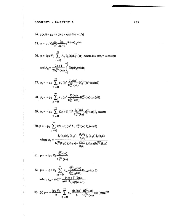
![ANSWERS - CHAPTER 6 704
ipcQo
2ha
oo
H(n2)(kr
) cos(n0)
ei°~t
n--O
~
.nr~ . .mn . -ia z
I~°V° E £ AmnC°Sl"~-x)c°sl"-~ y)e " ei°~t
84. p=
ab
n=0m=0
ab
whereAnm= enem f If(x,y)cos(~x)cos(-’~y)dydx
to 2 n2~ 2 m2~
2
a.d = a"7--
For f(x,y) = 1: Aoo = ab abc m= 0 fo r n, m * 0
andp = p c V
0 exp[- i o~(z - ct)]
2ptoVo
85. p= ~ £ E (Anmsin(n0)+Bnmc°s(n0))Jn(gtnmr)e-ia*~Zek°t
a
n=0m=l
2 a 2r~
r rsin(nO)]
Anm ~n
I-trim f f r f(r,
0) Jn (btnm
--) ~t ~ dO
where = 2 2 2
~ ~ a [cos(n0)J
B~ anm (gnm - n )Jn(~nm) 0
~nm
J~ (~nm) = 0, ~d ~ = ~2](https://image.slidesharecdn.com/advancedmathematicalmethodsinscienceandengineering-hayek-230318001731-2b30ece5/85/advanced-mathematical-methods-in-science-and-engineering-hayek-pdf-707-638.jpg)
![ANSWERS- CHAPTER 7 705
Chapter 7
(a) p/(p2 2)
(c) (p - a) / [(p 2 + b
21
(e) n! / (p +n+l
(b) 2ap/ (p2 + a2)2
(d) 2a2p/ (p4 + 4)
(f) a (p2 _ 2) / (p4 + 4a4)
2. In the followingF(p) = Lf(t):
(a) a F(ap)
(c) p F(p+a) - +)
(e) - dF(p+a)/dp
(g) (-1)n a dnF(ap)/dp
n
(i) -p dF/dp
(k) - (dF/dp)
(b) a F[a (p-b)]
(d) p d2F/dp
2
(f) (p - 1) 2 F(p-1)- (p - 1) f(0+)- f’(0
+)
(h) p (p- a) F(p-a) - p - f’(0+
(j) [F(p-a) - F(p+a)]
(1) F(p)
3. (a) {1 - pT e’PT/[1 - e-PT]}/p2
(c) [tanh(pT/4)] /
(e) {p[1 + e-PT/2]}
-1
(g) [p + ~0 / sinh (p~t/2co)]/(~2+ p2)
a
(b) p2 2 coth(p~z/2a)
(d) [~t p coth (pn/2) - 2]
(f) [2p cosh (pT/4)]
q
(a) at - ebt) / (a- b
(c) at - sin (at)
(e) t sin (at)
(g) sin (at) +at cos
(b) 1 - cos(at)
(d) sin (at) - at cos
(f) sin (at) cosh(at) - cos (at) sinh
(h) sinh (at) - sin
t
(a) y(t)= j’f_(t- x)sin(kx)dx+
Ac
os(k!)+ ~s in(kt)
0
t
(b) y(t)= ~yf(t-x)sinh(kx)dx+Acosh(kt)+--~sinh(kt)
0
(c) y(t) = ~ [cosh(at) - cos (at)] +~ [sinh (at) -
2a" 2a
J
t
(d) y(t)= 2a-@ff(t-x)(sinh(13x)-sin(13x))dx
0
t
(e) y(t)= if -x-2e-2x +e-3X]f(t-x)dx
0
t
(f) y(t)= ~[e-X-e-2X-xe-2X]f(t-x)dx
0
t
(g) y(t) 1 f x3e_xf(t - x)
0](https://image.slidesharecdn.com/advancedmathematicalmethodsinscienceandengineering-hayek-230318001731-2b30ece5/85/advanced-mathematical-methods-in-science-and-engineering-hayek-pdf-708-638.jpg)
![ANSWERS - CHAPTER 7 706
t
(h) y(t) =J -xf(t- x) dx
0
(i) y(t) -2t (1 ÷ 2
t) + Ao (t - t o) e-2(t-t°)H(t - to)
(j) y(t) =t t - e-2t
(k) y(t) =3t- e2t] + A[e3(t-t°) - e2(t-t° ) ] H(
t - 0)
(a) y(t)=
(b) y(t)=
(c) y(t)=
(d) y(t)=
0
(e) y(t)
1
(f) y(t)=
(g) y(t)=
(h) y(t)=
(i) y(t)
(j) y(t)
2 (t-to)/2 +~(t_to)e-2(t-to)_2e-2(t=to)]H(t_to)
-~e 25
A[1 - t2/2]
3 et/2 - e-t / 2
t
f(t - x)h(x)dx whereh(x) -1[p2 + k2_ G(p
)]-l, and G (p) = L g
[1 - at] e
"2at
t
f[4 e-4x - e-x ] f(t- x)
0
A
[2 (a- 1) -2t -(a- 2) -t - a e-at] + B[2 e-2t- e-t ]
(a- i) (a-
t
fcos(x)f(t x)dx
0
t
~e
ax (x) f(t - x)
cos
0
t
f(x-x ~/2)e-x f(t-x)dx
0
(a) x(t) = [-2U+ (U+ V)cosh (at) + (U- V)cos (at)] 2)
y(t) =[-2V+ (U+ V)cosh (at) + (V- U)cos (at)] 2)
(b) x(t) =y(t) -t+ t e-t
(c) x(t) t + tet, y(t)-- 3et +2t et
t
(d) x(t) -~[g(t) - f (t )] + --~-3(t-x)/2 [f(x) +g(x)]
2 4~
0
t
y(t) =½[f(t) - g(t)] +41---3(t-x)/2 [f(x) + g(x)] dx
0](https://image.slidesharecdn.com/advancedmathematicalmethodsinscienceandengineering-hayek-230318001731-2b30ece5/85/advanced-mathematical-methods-in-science-and-engineering-hayek-pdf-709-638.jpg)
![ANSWERS - CHAPTER 7 707
o
10.
11.
12.
t t
(e) x(t)= -~ (sin (x)-sinh(x))g(t-x)dx+-~ ~(sin(x)+ sinh(x))f(t-
0 0
t t
y(t)= ½~(sin(x)-sinh(x))f(t-x)dx+ ½~(sin(x)+ sinh(x))g(t-
0 0
t
(0 x(0 =J [cosh(x) f(t - x)- sinh (x) x)]
0
t
J [cosh(x) g(t - x)- sinh(x) f(t -
y(t)
0
(g) x(t) = ~9[(g- B)+o - Xo)]e2t + ~[A+ B-2(0 +Xo)]e-2t
+[(A+ B)-2(x 0 + yo)]e -t + ~[-(A+2B)+ 4(yo +2Xo)]te
-t
y(t) = ~-~- [(B - A)+ o - yo)]e2t + ~[A
+ B- 2(yo+ Xo)
-2t
+[(A+B)-2(x 0 +yo)]e -t +~[-(B+2A)+4(x 0 +2yo)]te
-t
Ac{_e_bX
sinh (bc(t - to)) H(t- to) + sinh (bc(t - to - x)) H(t
y(x,t) =
c c
1
X+Xo]
y(x,t) = -~Cyo {H[t- o
- +H[t-to + x-x°]
- Hit- to + x - xo ]H[x - xo] + H[t- to - x- xo ]H[x - xo] }
Cx-xo): !_x_+.xo)2.]~H(t_,o)
T= 7-Lr~.t-_ to)" exp[. -]- exp[
4K(t- to) 4K(t- to)
y(x,t) = Yo(x-.~)2 H(t)+ Y0C2t2+ ~-~ {(t-~)H(t-X)_c (t+ X)}c L f (t,x)
where~,x) = f(t + 2L/c, x) is a periodic function, definedoverthe first period
fl(t,×) = (t - _x)H(t - _x)+(t + _x)+(t- 2L - x)H(t-
C C C C ~
+(t 2L+X)H(t 2L+x)+2(t-L-X)H(t-L-x)+2(t-L+X)H(t-L+x)
C C C C C C](https://image.slidesharecdn.com/advancedmathematicalmethodsinscienceandengineering-hayek-230318001731-2b30ece5/85/advanced-mathematical-methods-in-science-and-engineering-hayek-pdf-710-638.jpg)
![ANSWERS - CHAPTER 7 708
13. y(x,t) = 2 o (t-x/c) H(t-x/c) -
14. y(x,t) =Yof(t,x)
where
f(t,x) -- f(t + 2L/c,x) is a periodicfunction,def’med
overthe first period
fl(t,x) = -H(t- L-X)+H(t- L+X)-H(t 2L-Xl+H(t---x)
C C C C
15. y(x,t) = YO
H(t - x) + c Posinh [cb(t- o -x)] H(t - o - x)
c bTo c c
-~T~sinh [cb(t - to)]e-bx H(t - to)
x
2
16. y(x,t) = Toerf( 4~Kt)+ To 4~K~(t~-to)-3/2 exp[-4K(t_to)]H(t-to)
17. T(x,t)-~ eKb2t{ebx
x b.~-]}
= -N erfc [2--~ + b~’l+ e-bx erfc [2---
~-
+ T
OeKb2te-bX
18. y(x,0 = [ee~(t-x/c)- 1] [H(t-x/c)]/~t
19. y(x,t) = - (t-x/c) o + ao(t-x/c)/2] H( t-x/c) +
20. T(x,0 -- TO{erfc( x--~)-et’x+b2V:terfc(_ x,._ + b4-K-’i’)} + QoK H(t-
2 4Kt 2 4Kt
- Q°KH(t- t°) {erfc (2 ~/K(~- )- ebx +b2K(t-to)erfc t ’2~ x
)-b K(~)}
21. T(x,0 = TOerfc(---~x~)+ KQ0(1-e-at) - KQ0erfc(--x~)
24Kt ak ka 2~/Kt
+--~e-at { e-iX4~7-~
erfc (2---~-- i 4"~)+eiX4~7-fferfc(2-~KtK
t + i ~]~’)}
22. y(x,t) = ~ {H[t - to - x -cX°] _ Hit - o +x -cx° ] )H[
x - x o]+ f(t)
where
f(t) = f(t +2L/c)is a periodicfunction, definedoverthe first period
fl(t) = H[t- to +x - xo ]_.H[t - to - x +xo ]
C C
-Hit-to 2L-x-x°]+H[t-to 2L+x-x°’]
C C](https://image.slidesharecdn.com/advancedmathematicalmethodsinscienceandengineering-hayek-230318001731-2b30ece5/85/advanced-mathematical-methods-in-science-and-engineering-hayek-pdf-711-638.jpg)
![ANSWERS - CHAPTER 7 709
23. y(x,t) = ~ {f(t)+ at - sin (at)}
a"AE
f(t) = f(t + 2L/c)is a periodicfunction,
definedover~hefirst period
as:
f~(t) =- [a(t - x) _ sin (a(t - x))] H
+[a(t- L + X)-sin(a(t- L + x))]I-I(t-
C C C
- [a(t - L - x) _ sin (a(t - L - X))l H(t -
C C
+[a(t - 2L--~Z-x)- sin(a(t - 2L- x))lH(t 2L
24. T(x,t)= T°erfc(~~)H(t-a)[4t-a-1]-’~9-terfc(2--’~)a
+ KQ° erf (~)H(t-
k 24~¢(t- to)
~sinh (bc(t- ~))
25. y(x,t) = A[[
bc
where A = Po a c
2
(a2 + b2c2)T0
sin (a(t- x)) . }
~ ]H(t_x)_[.sinh(bct) sin (at)
a c cb a
x
26. T(x,t) = -QKt[l+4erfc(.~-)]+T 0 x(t-to)-3/2 e-x~/[4K(t-to)]H(t
2.~-ff
-to)
27. y(x,t) = Y0cos (b(t - x))H(t - x) + FoC2~
[at -at]
c c AEa"
F°c2 [a t x. -a(t--x)
X)
~ ( --~)-l+e ¢ ]H(t-
t
28. T(x,t) = -~ H(t-to)- F K’~=~-x’/f4Ku] u-l 12 (t- u)e-a(t-u) du
0
29. y(x,t) = AH(t - x/c) - Yocosh (cb(t-x/c)) H(t-x/c) e’bx cosh (cbt)
30. T(x,t) = - KQo
a (1 - cos (at)) - 4Toterfc
t
,4"ffQoax
f[H(t u)
+ 44-~ J
- - cos(a(t- u))] -3/2 e-x2/t4Kul du
0](https://image.slidesharecdn.com/advancedmathematicalmethodsinscienceandengineering-hayek-230318001731-2b30ece5/85/advanced-mathematical-methods-in-science-and-engineering-hayek-pdf-712-638.jpg)
![ANSWERS -- CHAPTER 8 710
Chapter 8
o
g(xl~) = - sin x cos ~ + sin x sin ~ tan 1 + sin (x-~) H(x-~)
y(x) -- x - sin x / cos
g(X 1~)= ~n {[~n- ~-n]xn +[xn~ -n - x-n~n]H(x-~)}
3. g(X I ~) = 2n~{[~n -- ~-n] xn + [xn~-n -- x-n~n] a(x -
sinh (kx) sinh (k(L-
4. g(x I~)= +--’sinh(k(x-~))H(x-~)
k sinh (kL) k
6. g(xI~)=-~(x-~)3H(x-~)-2~L ~x2(L-~)2+6~L x3(L-~)2(L+2~)
7. g(xl~):-~(xl _~>3H(x_~>_~L~X(L-~)(2L-~>+~LX3(L-~>
sin (kx) sin(k(L 1
8. (a) g(xl~)= + "--sin(k(x-~))H(x-~)
ksin(kL) k
n=l
sin (nr~x/ L)sin(nr~ /
(i)
(a)
(b)
g(x I ~) = 2-~[sin (J3(x- ~)) - sinh (~(x- ~))]
~ ~shah(~x) sinh (~(L - sin (l~x) sin (~(L
- ~))
+
2~3 [ sinh (~L)
2 ~ sin (nnx / L) sin (nu~ /
g(x I~) =
~4 _ n4~4 / L
4
n=l](https://image.slidesharecdn.com/advancedmathematicalmethodsinscienceandengineering-hayek-230318001731-2b30ece5/85/advanced-mathematical-methods-in-science-and-engineering-hayek-pdf-713-638.jpg)
![ANSWERS -- CHAPTER 8 711
9
where:
(it)
(a)g(x I ~) =2-~[sin (13(x- ~)) - sinh (]3(x- ~))]
+ ~ {C~[sin (~3x)- sinh (~x)] + C2[cos(~x)- cosh
C
1 =
[sinh(I3(L- ~)) - sin (I3(L- ~))] [sin (I~L)+sinh
[1 - cos (~L)cosh(~L)]
[cosh(~(L- ~)) - cos (~(L- ~))] [cos(~L)-"cosh
[1 - cos(]3L)cosh(]3L)]
C2 =
[sinh (~(L- ~)) - sin (~(L - ~))] [cos (~L)-
[1 - cos (~L)cosh(I3L)]
+ [cosh(~(L- ~))- cos (~(L- ~))] [sin (~iL)- sinh
[1 - cos ~L)cosh (~L)]
(b) Eigenfunctions
{~n(X) are:
cosh(~ n’-’~"~ -- COS(O~n~I?°St
’c-
~7- ~°s" t-c- ~/
where,cos (eln) cosh(~tn) = 1, and with o =
0.Sothat g(xl~) is:
OO
X~,¢.(x)¢.(~)
g(x I~)= ~r~ Nn (l~ 4 -IXn
4/L4)
L
where Nn= J’,n2(x)dx
0
10. (a) g(xl~) = n Jn(kx) [j~(k)yn(k~)_jn(k~)yn(k)
]
2 Jn(k)
-- -~ [Jn (kx)
Yn(k~)
- J n (k~)
Yn(kx)]H(x
- ~)
m~ Jn(knmx) Jn(knm~)
(b) g(xl~) = 2 2 , 2
= 1 - knm)[Jn(knm)]
whereJn(knm)=](https://image.slidesharecdn.com/advancedmathematicalmethodsinscienceandengineering-hayek-230318001731-2b30ece5/85/advanced-mathematical-methods-in-science-and-engineering-hayek-pdf-714-638.jpg)
![ANSWERS .. CHAPTER 8
11. (a) g(x I ~) sin (kx)sin (k(l - ~))
kx~sin (k)
sin (k(x - ~)) H(x
2 sin (nr~x) sin (n~)
n=l
712
12. g(x I~)= ~ {e-rl(x+[) sin [rl(x +~)+ ~/41_ e-~lx-~l sin[rll ~ I+rc/4]}
where
~l= 7 /
13. (a) g(xl ~): ~ -~lx sinh (~) -rIG sinh01x)]H(x- ~)+ sinh (rlx) -~ }
whererl = 4"~ - k2
(b) g(xl~)= ~{[eirlx sin(rl~)-ein~sin(rlx)]H(x_~)+sin(rlx)ei~l~
where rl = ~ - 7
(c) g(xl~) = x - (x-~)
14. g(xl~) = x - (x-~) H(x-~)
X oo
T(x)=I +j’ ~ f(~)cl~ + xff(~)cl~
0 x
15. g(x I~) = 4~[ieiB(x+~)- e-B(x+~
) - ieiBIx-~I + e-BIx-~
I]
16. g(x I~) =~3 [-ieil~(x+[) + e-I~(x+[)- ieil~lx-[I +e-I~lx-[
I]
18.](https://image.slidesharecdn.com/advancedmathematicalmethodsinscienceandengineering-hayek-230318001731-2b30ece5/85/advanced-mathematical-methods-in-science-and-engineering-hayek-pdf-715-638.jpg)
![ANSWERS -- ~CHAPTER 8 713
"
_ 1.~_ ~e_al(x+~)/4~cos (rl(x + ~)
19. (a) g(xl~)= 2~13 , ~/~ ~-)
+ e-rllx-~l/’4~ cos (~ - ~)} 1~ = ()A - 1/4
~) g(x I ~) = ~r-ie i~(x+[) + e-~(x+[) - iei~lx-[I + e-~lx-~l] ~ = (~4 _ ~)l/4
4~3 ~
1 e_rllx_~l
21. (a) g(x I~)
(b) g(xl~) = ~i ei~lx-~l
2rl
(c)g(x
I~)=- ½
~x-
22. g(xl~)=-llx-~l
2
23. g(xl~)-~3 [-te’l]lx ~l+e-I~lx-[I]
24.
1 e_nrx_U/4~ . -
(a) g(x I~) =- ~ sm(~2 ~ I +-~)
(b) g(x I~)- 4--~3 ’ntx ~t +e ntx~]
1
(c)g(x
I ~)=- ~Ix-
25. g(xl~) = - log (rl)
26. g(xl~) = Ko(~[
) / 2r~ r1 =Ix - ~1
27. g(xl~)= i H(ol)(krl) / 4
28. (a) g = ~Ko(rlr
)
29. g(xl~) = r12(1 - log (rl)) rI = Ix- ~l](https://image.slidesharecdn.com/advancedmathematicalmethodsinscienceandengineering-hayek-230318001731-2b30ece5/85/advanced-mathematical-methods-in-science-and-engineering-hayek-pdf-716-638.jpg)
![ANSWERS -- CHAPTER 8
30. g(xl~) = kei(~rl) / r1 = Ix - ~1
714
31.
8~
2 Ko(rlq)]
rl = (k4 ,~4)1/4 rI =Ix - ~1
(a) g = - [iH(o1)(fIr
1) - ~ -
I
(b) g = 2-~kei(rlq) ~ = (~/1_k4)1/4 rI =Ix- ~1
32. Solution in eq. (8.103)
33. Solution in eq. (8.101)
34. Solution in eq. (8.118)
35. Solution in eq. (8.115)
36. g(x,tl~,x) = i~ H(t - x) {(1 - i) erfc [a(l- i)] + (I + i) erfc [a(l
Ix-El
a=~
37. g(x,tl~,x)=
A(r,t)
1 1 ~ sin x dx .H(t- x)
-~÷T-~ -~-
0
~o (-1)"~,t)
- ~ + H(t
8c (2n +1)(2n+
A(r,t)
r?
4x(t-x)
39. G= l+71[x+~-Ix-~l]
40. Usethe coordinate systemin Section 8.26 by deleting the y-coordinate.
1 d
(a) o= ~Iog(~)
(b) G =--~ log(rl2r~)
41. Usethe coordinate systemof Section 8.32 in twodimension,i.e. delete the y-
coordinatesuch that x _>0. Let:
(a) G=-~.~ log(qr2r3r
4)
(c) G= -~ log (~)
g2= -~’~log(r3), = -~
’~ log (r 4)
(b) G=- ~l---log(rlr3
zn r2r
4
(d) G--~-1 log(fir4 )
2n r2r
3](https://image.slidesharecdn.com/advancedmathematicalmethodsinscienceandengineering-hayek-230318001731-2b30ece5/85/advanced-mathematical-methods-in-science-and-engineering-hayek-pdf-717-638.jpg)
![ANSWERS -- CHAPTER 8
42. Usethe coordinate systemof Fig 8.9, section 8.32
1 ±)
Ca)C-- 1<±+1+_+
4n r 1 r
2 r 3 r4
1 (1 1 +1)
r2 r3r4
(c) G= 1__(1+ 1 1
4r~ q r 2 r 3 r
4
1 (1 1 +1_1)
r2r3 r4
i ta(1)rt.. ~ i H(1)rt.. x, ~ _ i H(1)~. ), ~ ~H(01)0cr4),
43. Define g = ~-,,0 ~’~ l J, gl = =
~" 0 ~2J s2-~" o ~"~3 s3
Coordinate system as in Problem41.
(a) G=g + gl + g2 + g3
Co) G=g-gl-g2+g
3
(c) G=g + gl - g2"
(d) G=g-gl +g2-g3
44. Usethe coordinates in Fig 8.9, Section 8.32.
eikrl eikr2 eikr~ eikr~
g = 4~q g~ 4m.
2 g2 4r~r
3
g3 4~.r4
(a) G=g+gl +g2 +g3
(b) G=g-gl-g2+g
3
(c) G=g+gl-g2-g3
(d) donein section 8.32
715
45 Definethe followingradial distances:
rl2 = (x- ~)2 + (y_ 1])2 + (z-
r22= (x- ~)2+(y_ 1.1)2 +(z
r32 = (x- ~)2 +(y + TI)2+ (z-
r42 = (x + ~)2+ (y_ 1~)2+ (z-
r~=(x-~)2+(y+~)2+(z
r6
2=(x+~)2
+(y.TI)2
+(z+~)2
r7
2=(x+ ~)2
+(y+ 1~)2
+(Z-~)2
r8
2=(x+ ~)2+(y+rl)2++ ~)2](https://image.slidesharecdn.com/advancedmathematicalmethodsinscienceandengineering-hayek-230318001731-2b30ece5/85/advanced-mathematical-methods-in-science-and-engineering-hayek-pdf-718-638.jpg)
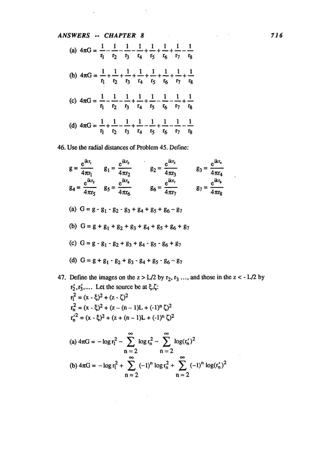
![ANSWERS -- CHAPTER 8 717
48. Define:
r? = (x - ~)2+ (y _ ~)2+(z
rn2 = (x- ~)2 +(y_ 11)2+ (z - (n - 1)L n ~)2
r~2 = (x- ~)2 +(y. ~1):~+ (z + (n - 1)Ln
= ±+ --+
rl = rn =
rl n=2 rn n=2 rn
49. Usesameradial distances as in Problem47
(a) ~iG=H~)(~)+ ~ H~)(~)+
n=2 n=2
~) ~iG=H~)(~)- Z (-1)"H~)(~)- E (-1)"H~)(~)
n=2 n=2
50. Usesameraidal distances as in Problem48
eikrl ~ eikr* ~ e~kr~
(a) 4r~G = ~ ~ + --
q n=2 rn n=2 r~
(b) 4~G= ~- (- 1)neikr* (-1)neikr~
r
1 r
n r~
n=2 n=2
i r"(1)"l~
’ - H(02)(k
]
51. O=~txl 0 t 1~
(a) For interior regionp,r1 < a, ~,r2 > a, ~ = a2/p
(b) For exterior regionp,r1 > a, ~,r2 < a, ~ = a2/p
52. Define:
rl ~ =r2 + p2 - 2rp cos (0- ¢)
r~ -- r2 + p2_ 2rp cos (0 + ~ - 2n/3)
r3~ = r2 + pg__ 2rp cos (0 - ¢- 2~/3)](https://image.slidesharecdn.com/advancedmathematicalmethodsinscienceandengineering-hayek-230318001731-2b30ece5/85/advanced-mathematical-methods-in-science-and-engineering-hayek-pdf-720-638.jpg)
![ANSWERS - CHAPTER 9 719
Chapter 9
(k- 0(k-2)(k3) -I
1. F(k,x)- xk-1 e -x [1+ k- 1 + (k- 1)(2k- 2)
-
~-
L x x ~ "’"
2. same as problem 1.
3. El(Z)- -z ~L,(-1)k k.~-.
I"
zk+l
k=O
o
n(n + I)n(n + 1)(n +
z 2 z
3
(2k)!
5. f(z)- ~(-1)k z2k+
1
k=O
(2k 1)!
6. g(z)- E (-1)k +
z2k+2
k=O
- e 1+ ~ (-1)
m
erfc(z) ~---~ m=l ~z~-) ~ ]
9. same as problem 8.
10.
q = 4v
2
11. sameas problem 10o
12. Kv(z)~ "~-’ze-Z{1+~zl (q- 1)(q- 32
)2! (8z)
2
q = 4V
2
(q - 1)(q - 32)(q- 52) ]
+ 3!(8z)
3 +"’"](https://image.slidesharecdn.com/advancedmathematicalmethodsinscienceandengineering-hayek-230318001731-2b30ece5/85/advanced-mathematical-methods-in-science-and-engineering-hayek-pdf-722-638.jpg)
![ANSWERS - CHAPTER 9
13. sameas problem 12.
14. sameas problem 12.
15. U(n.z) ~ -z’/4 z-n{1
n(n + 1) n(n+ 1)(n+ 2)(n+3)
2z 2 ~
2, (2z2)
2
16. sameas problem 15.
e in/4 1
0o (_i)n+ 1 r(n +
17. F(z) ~ ~÷~ eiZ’
E z~n+
1
n=O
18. O(x) ~ 1-~
e-x" ~ (-1) k r(k + 1/2)
~
z_~ x2k+l
k=0
19. Sameas problem 8
20. Same
as 10 for H(v
I),H(v2)(z)
=H(vl)(z)
21. Sameas 12 for K~(z)
(q - 1)(q
- 3~) (q - 1)(q - 3:~)(q - 5
~)
2!(8z)
2 3!(Sz)
3
720
q = 4V
2
22.
23. Ha)(1)(~)seco0 ~ exp[im) (tano~-ot)-i~/4] (- i)k uk (t’~)
k = 0](https://image.slidesharecdn.com/advancedmathematicalmethodsinscienceandengineering-hayek-230318001731-2b30ece5/85/advanced-mathematical-methods-in-science-and-engineering-hayek-pdf-723-638.jpg)
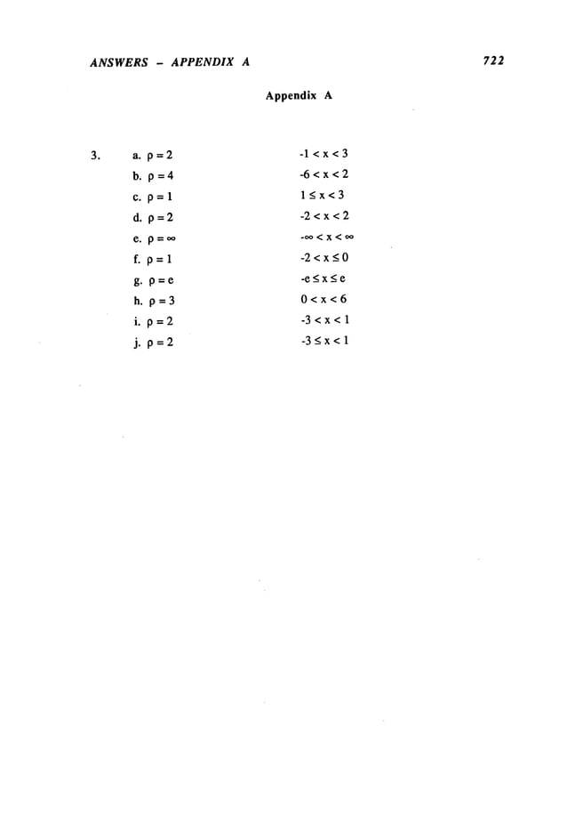


![[W]-REFERENCIA-Paul Waltman (Auth.) - A Second Course in Elementary Different...](https://cdn.slidesharecdn.com/ss_thumbnails/w-referencia-paulwaltmanauth-230516025940-c93e36a9-thumbnail.jpg?width=640&height=640&fit=bounds)


![Polymer [ बहुलक ] Chemistry Notes PDF - Irfanullah Mehar - JJ Sir Chemistry.pdf](https://cdn.slidesharecdn.com/ss_thumbnails/polymerchemistrynotespdf-irfanullahmehar-jjsirchemistry-260210172118-3f9b37f7-thumbnail.jpg?width=640&height=640&fit=bounds)


