This document provides an overview of a book on adaptive approximation based control. The book aims to unify various approaches to controlling nonlinear systems, including neural, fuzzy, and traditional adaptive control methods. It discusses using function approximators like neural networks to model unknown system nonlinearities, and adjusting the approximator parameters online through a stable training algorithm to achieve control objectives like tracking. The book covers approximation theory, common function approximation structures, parameter estimation methods, nonlinear control architectures, and applies these concepts to problems like aircraft control.


![NONLINEAR SYSTEMS 3
to inaccuracies or intentional model simplifications, constitute one of the key motivations
for employing adaptive approximation-basedcontrol, and thus are crucial to the techniques
developed in this book.
In general, the objectives of a control system design are:
1. to stabilize the closed-loop system;
2. to achieve satisfactory reference input tracking in transient and at steady state;
3. to reduce the effect of disturbances;
4. to achieve the above in spite of modeling error;
5. to achieve the above in spite of noise introduced by sensors required to implement
the feedback mechanism.
Introductory textbooks in control systems provide linear-based design and analysis tech-
niques for achieving the above objectives and discuss some basic robustness and imple-
mentation issues [61, 66, 86, 1401. The theoretical foundations of linear systems analysis
and design are presented in more advanced textbooks (see, for example, [lo, 19,39, 130]),
where issues such as controllability, observability, and model reduction are examined.
1.2 NONLINEAR SYSTEMS
Most dynamic systems encountered in practice are inherentlynonlinear. The control system
design process builds on the concept of a model. Linear control design methods can some-
times be applied to nonlinear systems over limited operating regions (i.e., 2)is sufficiently
small), through the process of small-signal linearization. However, the desired level of
performance or tracking problems with a sufficiently large operating region 2)may require
in which the nonlinearities be directly addressed in the control system design. Depending
on the type of nonlinearity and the manner that the nonlinearity affects the system, various
nonlinear control design methods are available [121, 134, 159, 234, 249, 2791. Some of
these methods are reviewed in Chapter 5.
Nonlinearity and model accuracy directly affect the achievable control system perfor-
mance. Nonlinearity canimpose hard constraintson achievable performance. The challenge
of addressing nonlinearities during the control design process is further complicated when
the description of the nonlinearities involves significant uncertainty. When portions of the
plant model are unknown or inaccurately defined, or they change during operation, the con-
trol performance may need to be severely limited to ensure safe operation. Therefore there
is often an interest to improve the model accuracy. Especially in tracking applications this
will typically necessitate the use of nonlinear models. The focus of this text is on adaptively
improving models of nonlinear effects during online operation.
In such applications the level of achievable performance may be enhanced by using
adaptive function approximation techniques to increase the accuracy of the model of the
nonlinearities. Such adaptive approximation-based control methods include the popular
areas of adaptive fuzzy and neural control. This chapter introduces various issues related to
adaptive approximation-based control. This introductory discussion will direct the reader
to the appropriate sections of the text where more detailed discussion of each issue can be
found.](https://image.slidesharecdn.com/adaptive-approximation-based-controlcompress-230219164415-f6eb4a64/85/adaptive-approximation-based-control_compress-pdf-21-320.jpg)
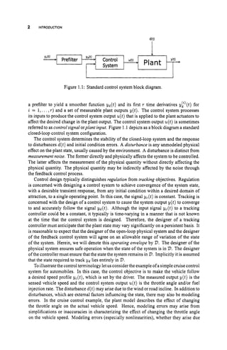
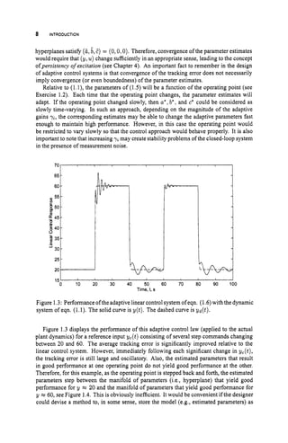
![4 INTRODUCTION
1.3 FEEDBACK CONTROL APPROACHES
To introduce the concept of adaptive approximation-based control, consider the following
example, where the objective is to control the dynamic system
in a manner such that y ( t ) accurately tracks an externally generated reference input signal
yd(t). Therefore, the control objective is achieved if the tracking error Q(t)= y ( t ) - yd(t)
is forced to zero. The performance specification is for the closed-loop system to have a
rate of convergence corresponding to a linear system with a dominant time constant T of
about 5.0 s. With this time constant, tracking errdrs due to disturbances or initial conditions
should decay to zero in approximately 15 s (= 37). The system is expected to normally
operate within y E 120,601, but may safely operate on the region 23 = {y E [0,loo]}. Of
course, all signals in the controller and plant must remain bounded during operation.
However, the plant model is not completely accurate. The best model available to the
control system designer is given by
where f,(y) = -y and go(y) = 1.0+0 . 3 ~ .
The actual system dynamics are not known or
available to the designer. For implementation of the following simulation results, the actual
dynamics will be
f(y) = -1 -0.01y2
Therefore, there exists significant error between the design model and the actual dynamics
over the desired domain of operation.
This section will consider four alternative control system design approaches. The ex-
ample will allow a concrete, comparative discussion, but none of the designs have been
optimized. The objective is to highlight the similarities, distinctions, complexity, and com-
plicating factors of each approach. The details of each design have been removed from this
discussion so as not to distract from the main focus. The details are included in the problem
section of this chapterto allow further exploration. These methodologies and various others
will be analyzed in substantially greater detail throughout the remainder of the book.
1.3.1 Linear Design
Given the design model and performance specification, the objective in this subsection is
to design a linear controller for the system
y(t)= h(y(t),u(t))
= - y ( t ) +(1.0 +O.Sy(t))u(t) (1.3)
so that the linearized closed-loop system is stable (stability concepts are reviewed in Ap-
pendix A) and has the desired tracking error convergence rate. This controller is designed
based on the idea of small-signal linearization and is approximate, evenrelative tothe model.
Section 1.3.3 will consider feedback linearization, which is a nonlinear design approach
that exactly linearizes the model using the feedback control signal.](https://image.slidesharecdn.com/adaptive-approximation-based-controlcompress-230219164415-f6eb4a64/85/adaptive-approximation-based-control_compress-pdf-22-320.jpg)
![12 INTRODUCTION
80
40
4
P
20
i
0 10 20 30 40 50 60 70 80 90 100
Time, t, s
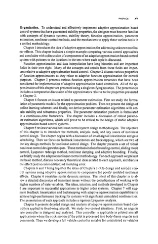
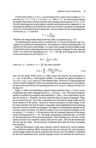
Figure 1.6: Performance of the approximation-based control system of eqn. (1.19)-(1.21)
with the dynamic system of eqn. (1.1).
ci = (i - 1)5, f o r i = 1,. . . ,21.
This simulation uses the actual plant dynamics. Initially, the tracking error is large, but as
the online data is used to estimate the approximator parameters, the tracking performance
improves significantly.
It is important that the designer understands the relationship between the tracking error
and the function approximation error. It is possible for the tracking error to approach zero
without the approximation error approaching zero. To see this, consider (1.22). If the last
three terms sum to zero, then ij will converge to zero. The last three terms sum to zero
across a manifold of parameter values, most of which do not necessarily represent accurate
approximations over the region D. If the designer is only interested in accurate tracking,
then inaccurate function approximation over the entire region 2)may be unimportant. If
the designer is interested in obtaining accurate function approximations, then conditions
for function approximation error convergence must be considered.
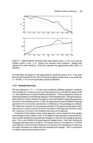
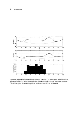
Figure 1.7 displays the approximations at the initiation (dotted) and conclusion (solid)
of the simulation evaluation, along with the actual functions (dashed). The simulation was
concluded after 3000 s of simulated operation. The first 100 s of operation involved the
filtered step commands displayed in Figure 1.6. The last2900 sof operation involved filtered
step commands, each with a 10-sduration, randomly distributed in a uniform manner with
yc E [20,60]. The initial conditions for the function approximation parameter vectors were
defined to closely match the functions j oand go of the design model. The bottom graph
of Figure 1.8 displays the histogram of yd at 0.1-s intervals. The top two graphes show
the approximation error at the initial and final conditions. By 3000 s, both f and B have
converged over the portion of D that contains a large amount of training data. Nothing can](https://image.slidesharecdn.com/adaptive-approximation-based-controlcompress-230219164415-f6eb4a64/85/adaptive-approximation-based-control_compress-pdf-30-320.jpg)
![COMPONENTS OF APPROXIMATION BASED CONTROL 17
approximating function -this isreferred to as training in the neural network literature. The
parameters 6 are referred to in the (neural network) literature as the output layer parameters.
The parameters u are referred to as the input layer parameters. Note that the approximation
of eqn. (1.27) is linear-in-the-parameters with respect to 8. The vector of basis functions
4 will be referred to as the regressor vector. The regressor vector is typically a nonlinear
function of z and the parameter vector a.Specification of the structure of the approximating
function includes selection of the basis elements of the regressor 4, the dimension of 8,and
the dimension of a. The values of 8 and a are determined through parameter estimation
methods based on the online data.
Regardless of the choice of the function approximator and its structure, it will normally
be the case that perfect approximation is not possible. The approximation error is denoted
by e(z; 8,a)where
e(z; 6,U ) = f
(
z
)- f(z;8,a). (1.28)
If 8*and CT* denote parameters that minimize the m-norm of the approximating error over a
compact region V,
then the Minimum Functional Approximation Error (MFAE) is defined
as
e+(z) = e(z; 6', a*)= f(z)
- f
(
z
;
8*,a*).
In practice, the quantities e+,8' and a* are not known, but are useful for the purposes of
analysis. Note, as in eqn. (1.22), that e4(z) acts as a disturbance affecting the tracking error
and therefore the parameter estimates. Therefore, the specification of the adaptive approx-
imator f(z;8,a)has a critical affect on the tracking performance that the approximation-
based control system will be capable of achieving.
The approximator structure defined in eqn. (1.27) is sufficient to describe the various
approximators used in the neural and fuzzy control literature, as well as many other approx-
imators. Issues related to the adaptive approximation problem and approximator selection
will be discussed in Chapter 2. Specific approximators will be discussed in Chapter 3.
1.4.3 Stable Training Algorithm
Given that the control architecture and approximator structure have been selected, the
designer must specify the algorithm for adapting the adjustable parameters 6 and a of
the approximating function based on the online data and control performance.
Parameter estimation can be designed for either a fixed batch of training data or for
data that arrives incrementally at each control system sampling instant. The latter situation
is typical for control applications; however, the batch situation is the focus for much of
the traditional function approximation literature. In addition, much of the literature on
function approximation is devoted to applications where the distribution of the training
data in V can be specified by the designer. Since a control system is completing a task
during the function approximation process, the distribution of training data usually cannot
be specified by the control system designer. The portion of the function approximation
literature concerned with batches of data where the data distribution is defined by the
experiment and not the analyst is referred to as scattered data approximation methods
[84].
Adaptive approximation-based control applications are distinct from traditional batch
scattered data approximation problems in that:
0 the data involved in the parameter estimation will become available incrementally
(ad infinitum) while the approximated function is being used in the feedback loop;](https://image.slidesharecdn.com/adaptive-approximation-based-controlcompress-230219164415-f6eb4a64/85/adaptive-approximation-based-control_compress-pdf-35-320.jpg)
![20 INTRODUCTION
withp = G,
2. Analyze the linear control law of eqn. (1.4) and the linearized dynamics (above)
to see that the nominal control design relies on cancelling the plant dynamics and
replacing them with error dynamics of the desired bandwidth. Analyze the charac-
teristic equation of the second-order, closed-loop linearized dynamics to see what
happens to the closed-loop poles when p is near but not equal to 3.
3. Design a set of linear controllers and a switching mechanism (i.e., a gain scheduled
controller) so that the closed-loop dynamics of the design model achieve the band-
width specification over the region v E [20,60]. Test this in simulation. Analyze the
performance of this gain scheduled controller using the actual dynamics.
Exercise 1.2 This exercise steps through the design details for the linear adaptive controller
of Section 1.3.2.
Derive the error dynamics of eqns. (1.1 1)-( I.14) for the linear adaptive control law.
(Hint: add -tu +EIJ to eqn. (1.5)and substitute eqn. (1.6) for the latter term.)
Show that the correct values for the model of eqn. (1.5) to match eqn. (1.1) to first
order are:
y=y*,u=u*
Implement a simulation of the adaptive control system of Section 1.3.2. First, dupli-
cate the results of the example. Do the estimated parameters converge to the same
values each time TI is commanded to the same operating point?
Using the Lyapunov function
7
1 Yz 7 3
show that the time derivative of V evaluated along the error dynamics of the adaptive
control system is negative semidefinite. Why can we only say that this derivative is
semidefinite? What does this fact imply about each component of (a,5:Ib, Z)?
Exercise 1.3 This exercise steps through the design details of an extension to the feedback
linearizing controller of Section 1.3.3.
Consider the dynamic feedback linearizing controller defined as
where 5 = (y - Yd). This controller includes an appended integrator with the goal of
driving the tracking error to zero.](https://image.slidesharecdn.com/adaptive-approximation-based-controlcompress-230219164415-f6eb4a64/85/adaptive-approximation-based-control_compress-pdf-38-320.jpg)

![24 APPROXIMATIONTHEORY
be discussed through the remainder of this chapter. Section 2.2 discusses the problem
of function interpolation. Section 2.3 discusses the problem of function approximation.
Section 2.4 discusses function approximator properties in the context of online function
approximation.
2.1 MOTIVATING EXAMPLE
Consider the following simple example that illustrates some of the issues that arise in
approximation based control applications.
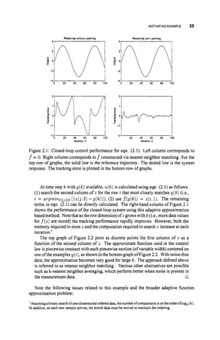
4 EXAMPLE2.1
Consider the control of the discrete-time system
z(k +1) = f(z(k))+u(k)
y(k) = +),
where u(k)is the control variable at discrete-time k, z ( k ) is the state, y(k) is the
measured output, the function f(z)
is not known to the designer, and the control law
is given by
The above control law assumes that the reference trajectory Yd is known one step in
advance. For the purposes of simulation in the example, we will use f(z)
= sin(z).
u(k)= Yd(k +1)-P [ Y d P ) - Y (k)l -f*(Y(k)). (2.1)
If f(y) = sin(y),then the closed-loop tracking error dynamics would be
e(k +1)= Pe(k),
where e(k)= yd(k) - z(k),which is stable for IpI < 1(in the following simulation
example we use p = 0.5). If f(y) # f(z),
then the closed-loop tracking error
dynamics would be
e(k + 1)= Pe(k) - [f(z(k))
- f(Y(W1. (2.2)
Therefore, the tracking performance is directly affected by the accuracy of the design
model f(z). The left hand column of Figure 2.1 shows the performance of this
closed-loop system when yd(k) = nsin(0.lk) and f(y) = 0.
When f(z)
is not known apriori,the designer may attempt to improve the closed-
loop performance by developing an online (i.e., adaptive) approximation to f
(
z
)
.
In
this section a straightforward database function approximation approach is used. At
each time step k, the data
4 k ) = [ M k - I))>Y(k - 1)1
will be stored. Note that the approach ofthis example requires that the function value
f(y(k - 1))must be computable at each step from the measured variables. This
assumed approach is referred to as supervised learning. This is a strict assumption
that is not always applicable. Much more general control approaches that do not
require this assumption are presented in Chapter 6. For this example, at time k, the
information in z(k)can be computed from available data according to
r(k)= [y(k) - u(k - 1). y(k - l)].](https://image.slidesharecdn.com/adaptive-approximation-based-controlcompress-230219164415-f6eb4a64/85/adaptive-approximation-based-control_compress-pdf-42-320.jpg)
![MOTIVATINGEXAMPLE 27
2
1.
L
0
._
P 0,
Y
L
+ -1.
-2
Response without Learning Response with Learning
41 I 21 I
2
$ 1 .
P O
s -1.
k
H
m
I -2
6 0
5
32w
-2
-4 0 50 100 150 200 iiw
-1
-2 0 50 100 150 200
Figure 2.3: Closed-loop control performance for eqn. (2.1)with noisy measurement data.
Left column corresponds to f = 0. Right column corresponds to f constructed via nearest
neighbor matching. In the top row of graphs, the solid line is the reference trajectory and
the dotted line is the system response.
stored in the data vector without noise attenuation. It is important to note that, as
we will see, methods to attenuate noise through averaging lead directly to function
approximation methods.
4.Function approximation problems are not well defined. Consider Figure 2.4, which
corresponds to the the data matrix z stored relative to Figure 2.3. If the domain of
approximation that is of interest is D = [-T, T ] ,
how should the approximation given
the available data be extended to all of D (or should it?). A quick inspection of the
datamightleadtothe conclusion thatthe function islinear. A more careful inspection,
noting the apparent curvature near !
z
; might result in the use of a saturating function.
From our knowledge of f(x)neither of these is of course correct. Extreme care must
be exercised in generalizing from available data in given regions to the form of
the function in other regions. The manner in which data in one region affects the
approximated function in another region is determined primarily by the specification
of the function approximator structure. The assumed form of the approximation
inserts the designer’s bias into the approximation problem. The effect of this bias
should be well understood.
5. From eqn. (2.2)the designer might expect that, as the database accumulates data,
then the (f -f)term and hence e should decrease; however,the control and function
approximation approach of this example did not allow a rigorous stability analysis.
The parametric function approximation methods that follow will enable a rigorous
analysis of the stability properties of the closed-loop system.](https://image.slidesharecdn.com/adaptive-approximation-based-controlcompress-230219164415-f6eb4a64/85/adaptive-approximation-based-control_compress-pdf-45-320.jpg)
![28 APPROXIMATION THEORY
Stored data
Y
Figure 2.4: Data for approximating f^ corresponding to eqn. (2.1) with noisy measurement
data.
Items 2 through 4 above naturally direct the attention of the designer to more general
fimction interpolation and approximation issues. The above nearest neighbors approach
can be represented as
k
j(2 : z(k))= Cz(i.
l)r#)i(Z : z ( k ) ) (2.3)
i=l
where thenotation f^(z
: z ( k ) )means the value off evaluatedat 2 given the data indatabase
matrix z at time Ic, and
where we have assumed that no two entries (i.e., rows) have the same value for z(j,2).
Note that by its definition, this function passes exactly through each piece of measured
data (i.e., f ( z ( i ,2 ) : z ( k ) )= z(i,1)).This is referred to as interpolation. Item 2 above
points out the fact that this approximation structure has k basis elements that are redefined
at each sampling instant. The computational complexity and memory requirements can be
decreased and fixed by instead using a fixed number N of basis elements of the form
where the data matrix z would be used to estimate 0 = [el,...,ON] and u = [ul,...,b ~ ] .
With such a structure, it will eventually happen that there is more data than parameters,
in which case interpolation may no longer be possible. After this instant in time, a well-
designed parameter estimation algorithm will combine new and previous measurements to](https://image.slidesharecdn.com/adaptive-approximation-based-controlcompress-230219164415-f6eb4a64/85/adaptive-approximation-based-control_compress-pdf-46-320.jpg)
![INTERPOLATION 29
attenuate the affects of measurement noise on the approximated function. The choice of
basis functions can affect the noise attenuation properties of the approximator. In addition,
the choice of approximator will affect the accuracy of the approximation, the degree of
approximator continuity and the extent of training generalization, as will be explained in
Section 2.4.7.
2.2 INTERPOLATION
Given a set of input-output data {(zj, yj) 1 j = 1,...,m; xj E R2";yj E R
'
}
, function
interpolation is the problem of defining a function f
(
z
)
: Rn + R1 such that f
(
z
,
)
= yj
for all j = 1,...,m. When f(z)is constrained to be an element of a finite dimensional
linear space, this is called Lagrange interpolation. The interpolating function f(z)can
then be used to estimate the value of f(z)
between the known values of f(zj).
In Lagrange interpolation with the basis functions {$i(z)}El,
N
f(z)= Cei4i(z)
= eT4(.) = 4 ( ~ ) ~ 8 , (2.6)
i=l
where 8 = [el,...16'N]T E RZN
and d(z) = [@1(z),
...,$N(z)IT : R2"+ RN. The
Lagrange interpolation condition can be expressed as the problem of finding 6' such that
Y = QT8.
Note that Q, = [$(.I), ...,4(zm)]
E RNxm.
The matrix QT is referred to as the interpola-
tion or collocation matrix. Much of the function approximation and interpolation literature
focuses on the case where n = 1. When n > 1and the data points are not defined on a
grid, the problem is referred to as scattered data interpolation .
A necessary condition for interpolation to be possible is that N 2 m. In online appli-
cations, where m is unbounded (i.e., zk = z(kT)),
interpolation would eventually lead to
both memory and computational problems.
If N = m and CP is nonsingular, the unique interpolated solution is
8 = (aT)-lY = Q,-TY. (2.9)
Nonsingularity of Q, is equivalent to the column vectors $(xi),i = 1,...,m being linearly
independent. This requires (at least) that the zibe distinct points. Once suitable N, 4(z),
yi, and z
ihave been specified, the interpolation problem has a guaranteed unique solution.
When the basis set {$j},"=, has the property that the matrix Q, is nonsingular for any
distinct {zi}El,the linear space spanned by {q$},"=, is referred to as a Chebyshat space
or a Haar space [79, 155, 2181. The issue of how to select 4 to form a Haar space has
been widely studied. A brief discussion of related issues is presented in Section 2.4.10.
Even if the theoretical conditions required for CP to be invertible are satisfied, if zi is near
z j for i # j, then Q, may be nearly singular. In this case, any measurement error in Y
may be magnified in the determination of 8. In addition, the solution via eqn. (2.9) may](https://image.slidesharecdn.com/adaptive-approximation-based-controlcompress-230219164415-f6eb4a64/85/adaptive-approximation-based-control_compress-pdf-47-320.jpg)
![30 APPROXIMATIONTHEORY
be numerically unstable. Preferred methods of solution are by QR, UD, or singular value
decompositions [991.
For a unique solution to exist, the number of free parameters (Lee,the dimension of 0)
must be exactly equal to the number mof sample points 2%.
Therefore, the dimension of the
approximator parameter vector must increase linearly with the number of training points.
Under these conditions, the number of computations involved in solving eqn. (2.9) is on
the order of m3floating point operations (FLOPS) (see Section 5.5.9 in [99]). In addition
to this large computational burden, the condition number of often becomes small as m
gets large.
As the number of data points m increases, there will eventually be more data (and
for m = N more degrees of freedom in the approximator) than degrees of freedom in
the underlying function. In typical situations, the data yi will not be measured perfectly,
but will include errors from such effects as sensor measurement noise. The described
interpolation solution attempts to fit this noisy dataperfectly, which is not usually desirable.
Approximators with N < m parameters will be over-constrained (i.e., more constraints
than degrees of freedom). In this case, the approximated function can be designed (in an
appropriate sense)to attenuate the effects of noisy measurement data. An additional benefit
of fixing N (independent of m)is that the computational complexity of the approximation
and parameter estimation problems is fixed as a function of N and does not change as more
data is accumulated.
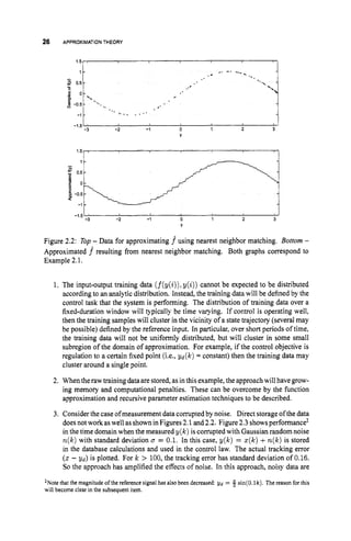
1 EXAMPLE2.2
Consider Figures 2.2 and 2.4. The former figure represents the underlying "true"
function (i.e., noise-free data samples). The latter represents noisy samples of the
underlying function. Interpolation of the data in Figure 2.4 would not generate a
reliable representation of the desired function. In fact, depending on the choice of
basis functions, interpolation of the noisy data may amplify the noise between the
data points. n
2.3 FUNCTION APPROXIMATION
The linear in the parameters3 (LIP) function approximation problem can be stated as: Given
a basis set {$J~(z)
: En --t Efor i = 1... N } and a function f(z): En + E1find a
linear combination of the basis elements f(x) = OT+(z) : En + E
l that is close to f.
Key problems that arise are:
0 How to select the basis set?
0 How to measure closeness?
0 How to determine the optimal parameter vector 0 for the linear combination?
In the function approximation literature there are various broad classes of function ap-
proximation problems. The class of problems that will be of interest herein is the develop-
ment of approximations to functions based on information related to input-output samples
'In general, the function approximation problem is not limited to LIP approaches; however, this introductory
section will focus on LIP approaches to simplify the discussion.](https://image.slidesharecdn.com/adaptive-approximation-based-controlcompress-230219164415-f6eb4a64/85/adaptive-approximation-based-control_compress-pdf-48-320.jpg)
![FUNCTIONAPPROXIMATION 31
of the function. The foundations of the results that follow are linear algebra and matrix
theory [99].
2.3.1 Offline (Batch) FunctionApproximation
Given a set of input-output data {(
z
i
,
yi), i = 1,...,m} function approximation is the
problem of defining a function f(z): ---t ?I?1 to minimize lY - Y/I where Y =
[yl,...,
y
,
I
T andY = [f(q),
...,f*(zm)lT.Thediscussionofthefollowingtwosections
will focus on the over and under constrained cases where 11. I/ denotes thep = 2 (Euclidean)
norm. Solutions for other p norms are discussed, for example, in the references [54,309].
2.3.1.1 Over-constrainedSolution Consider the approximator structure of eqn.
(2.6), which can be represented in matrix form as in eqn. (2.8). When N < m the problem
is over-specified (more constraints than degrees of freedom). In this case, the matrix @
defined relative to eqn. (2.8) is not square and its inverse does not exist. In this case, there
may be no solution to the corresponding interpolation problem. Since with the specified
approximation structure the datacannot be fit perfectly, the designer may instead select the
approximator parameters to minimize some measure of the function approximation error.
If a weighted second-order cost function is specified then
(2.10)
1
J(e)= 5(Y - Y ) ~ w ( Y
-Y )
which corresponds to the norm lYlb= iYTWY where W is symmetric and positive
definite. In this case, the optimal vector 8*can be found by differentiation:
1
2
~ ( 8 )= -(aTe-y)Tw(@Te
-Y ) (2.1I)
(2.12)
e* = (@W@T)-'@WY (2.13)
where it has been assumed that rank(@)= N (Lee,that @ has N linearly independent
rows and columns) so that @W@' is nonsingular. When the rank of @ < N (i.e., the
N rows of @ are not linearly independent), then either additional data are required or the
under-constrained approach defined below must be used. Since the second derivative of
J(8)with respect to 8 evaluated at 0' (i.e., @WQT),
is at least positive semidefinite, the
solution of eqn. (2.13) is a minimum of the cost function.
Eqn. (2.13) is the weighted least squares solution. If W is a scalar multiple of the
identity matrix, then the standard least squares solution results. Note from eqn. (2.12)
that the weighted least squares approximation error (@TO* - Y )has the property that it is
orthogonal to all N columns of the weighted regressor W a T .
Even when the rank(@)is N so that the inverse of (@WQT)
exists, the weighted least
squares solution may still be poorly conditioned. In such a case, direct solution of eqn.
(2.13)may not be the best numeric approach (see Ch. 5 in [99]). The condition number of
the matrix A (i.e., cond(A))provides an estimate of the sensitivity of the solution of the
linear equation Aa: = bto errors in b. If a(A) anda(A)denote the maximum and minimum
singular values ofA,then log,, (B)
provides anestimate inthe numberofdecimal digits
of accuracy that are lost in solving the linear equation. The function C = #isan estimate](https://image.slidesharecdn.com/adaptive-approximation-based-controlcompress-230219164415-f6eb4a64/85/adaptive-approximation-based-control_compress-pdf-49-320.jpg)
![FUNCTIONAPPROXIMATION 33
Since 6' is orthogonal to C,"=;'"
aidi by construction, llwll = ll6'll+ I/C,";" aidill which
is always greater than Il6'il. For additional discussion, see Section 6.7 of [29].
2.3.7.3 Summary This section has discussed the offline problem of fitting a function
to a fixed batch of data. In the process, we have introduced the topic of weighted least
squares parameter estimation which is applicable when the number of data points exceeds
the number of free parameters defined for the approximator. We have also discussed the
under-constrained case when there is not sufficient data available to completely specify the
parameters of the approximator. Normally in online control applications, the number of
data samples rnwill eventually be much larger that the number ofparameters N . Thisis true
since additional training examples are accumulated at each sampling instant. The results
for the under-constrained case are therefore mainly applicable during start-up conditions.
2.3.2 Adaptive Function Approximation
Section 2.3.1.1 derived a formula for the weighted least squares (WLS) parameter estimate.
Given the first k samples, with k 2 N , the WLS estimate can be expressed as
e k = ( @ k w k @ ; ) - ' @ k w k Y k
where @ k = [$(XI), ...,@ ( x k ) ] E R N x k ,
Y k = [ y l ,...,y k I T , and w k is an appropriately
dimensioned positive definite matrix. Solution of this equation requires inversion of an
N x N matrix. When the ( k+1)stsample becomes available, this expression requires the
availability of all previous training samples and again requires inversion of a new N x N
matrix. For a diagonal weighting matrix w k , direct implementation of the WLS algorithm
has storage and computational requirements that increase with k. This is not satisfactory,
since k is increasing without bound.
A main goal of subsection 2.3.2.1 is to derive a recursive implementation of that algo-
rithm. That subsection is technical and may be skipped by readers who are not interested in
the algorithm derivation. Properties of the recursive weighted least squares (RWLS) algo-
rithm will be discussed in subsection 2.3.2.2. Twoproperties that are critically important are
that (given proper initialization) the WLS and RWLSprovide identical parameter estimates
and that the computational requirements of the RWLS solution method are determined by
N instead of k.
2.3.2.7 Recursive WLS:Derivation The WLS parameter estimate can be expressed
as
(2.17)
In the case where w k = 1,p k is the sample regressor autocorre~ation
matrix and R k is
the sample cross-correlation matrix between the regressor and the function output. For
interpretations of these algorithms in a statistical setting, the interested reader should see,
for example, [133, 1641.
From the definitions of @, Y ,and W ,assuming that W is a diagonal matrix, we have
that
1
k k
e k = P L I R k , where P k = ' @ k w k @ L and R k = - @ k W k Y k .
Y k + l = [ yk ] @ k + l = [ @ k #k+l 1, and w k + l = [ L k + l ]. (2.18)
Y k + l
Therefore,](https://image.slidesharecdn.com/adaptive-approximation-based-controlcompress-230219164415-f6eb4a64/85/adaptive-approximation-based-control_compress-pdf-51-320.jpg)
![34 APPROXIMATIONTHEORY
Calculation of the WLS parameter estimate after the (Ic + 1)st sample is available will
require inversion of the @k+lWk+1@&1. The Matrix Inversion Lemma [99] will enable
derivation of the desired recursive algonthm based on eqn. (2.19).
The Matrix Inversion Lemma statesthat if matrices A, C, and ( A+BCD)are invertible
(and of appropriate dimension), then
( A+B C D ) - ~
= A-1 - A - ~ B
( D A - ~ B
+c-l)-lDA-'.
The validity of this expression is demonstrated by multiplying ( A+BCD) by the right-
hand side expression and showing that the result is the identity matrix.
Applying the Matrix Inversion Lemma to the task of inverting @k+lWk+l@L+l, with
Ak = @ k w k @ l , B = f$k+l, c = W k + l , and D = C$:+~,
yields
AL;l = ( @ k w k @ l f 4 k + l W k + l d ) l + 1 ) - 1
Ai;1 = Ail - AL14k+l(&+iAi14k+l +wi:i)-' 4i+;rlAk1. (2.21)
Note that the WLS estimate after samples k and (k+1)can respectively be espressed as
e k = Acl@kwkYkand ek+l = Ai:1@k+lWk+1Yk+l.
The recursive WLS update is derived, using eqns. (2.20) and (2.21), as follows:
ek+l = [A,' - Akl$k+l (&+lAild'k+l f w;;1)-' 4i+1Ak1]
[ @ k w k y k +$ k + l w k + l Y k + l ]
= e k - AL14k+l (&+lAL1d)k+l f wc:l)-' @kjiek
+ A i 1 4 k + l w k + l Y k + l
-Ai14k+l (4L+;1Ak14k+l
+w;:i)- d)k+l
T A-1
k +k+lwk+lYk+l
= e k - Ai14k+l (&+iA;'$k+l f w;:i)-' 4;+1ek
+AL1d%+i
[I- (&+1Ai14k+i +wi;l)-l d):flAi14k+i]
wk+iYk+i
= e k - Ail$k+i (&+1Ai14k+l +WL:l)-l #;+lek
+A,l$k+l (4kj1Ai1d)k+l
f wi:l)-'
[4L+1AL1$k+l +wL;l - 4;+1Ai14k+l]wk+lYk+l
= e k +Ai14k+1(&+lAkl$k+l +WF;1)-' ( Y k f l - 4L+iek) 3
= e k +A,' ( & + l A ~ l $ k + l +wi;i)-' $k+l (Yk+l - 4l+;,ek) 2
ek+l
ek+l (2.22)
where we have used the fact that (4L+;,Ai14k+l
+wii1) is a scalar. Shifting indices in
eqn. (2.21) yields the recursive equation for A i l :
(2.23)
2.3.2.2 Recursive WLS:Properties TheRWLSalgorithm isdefinedby eqns. (2.22)
and (2.23). This algorithm has several features worth noting.
Ail = A-' -A- T -1
k - 1 k l l @ k ( 4 k A k - l @ k f wc1)-l d)LAL:l.](https://image.slidesharecdn.com/adaptive-approximation-based-controlcompress-230219164415-f6eb4a64/85/adaptive-approximation-based-control_compress-pdf-52-320.jpg)
![FUNCTION APPROXIMATION 35
1. Eqn. (2.22) has a standard predictor-corrector format
ek+l= ek+n k $ k + l b k + l - gk+l:k) (2.24)
- 1
where RI, = A i l ($L+lAklI$k+l+wkil) is the estimate
of yk+l based on ek. The majority of computations for the RWLS algorithm are
involved in the propagation of Ail by eqn. (2.23).
2. The RWLS calculation only uses information from the last iteration (i.e., A i l and
8 k ) and the current sample (i.e., Yk+l and &+I). The memory requirements of the
RWLS algorithm are proportional to N , not k. Therefore, the memory requirements
are fixed at the design stage.
and $k+l:k =
3. The WLS calculation of eqn. (2.13) requires inversion of an N x N matrix. The
RWLS algorithm only requires inversion of an n x n matrix where N is the number
of basis functions and n is the output dimension off, which we have assumed to be
one. Therefore, the matrix inversion simplifies to a scalar division. Note that Ak is
never required. Therefore, A i l is propagated, but never inverted.
4. All vectors and matrices in eqns. (2.22) and (2.23) have dimensions related to N ,
not k. Therefore, the computational requirements of the RWLS algorithm are fixed
at the design stage.
5. Since no approximations have been made, the recursive WLS parameter estimate is
the same as the solution of eqn. (2.13),if the matrix A i l isproperly initialized. One
approach is to accumulate enough samples that A k is nonsingular before initializing
the RWLS algorithm. An alternative common approach is to initialize A;' as a large
positive definite matrix. This approximate initialization introduces an error in 81
that is proportional to IIAolI. This error is small and decreases as k increases. For
additional details see Section 2.2 in [154].
6. Due to the equivalence of the WLS and RWLS solutions, the RWLS estimate will
not be the unique solution to the WLS cost function until the matrix @k Wk@lis not
singular. This condition is referred to as @k being su8ciently exciting.
Various alternative parameter estimation algorithms can be derived (see Chapter 4).
These algorithms require substantially less memory and fewer computations since they do
not propagate A i l , the tradeoff is that the alternative algorithms converge asymptotically
instead of yielding the optimal parameter estimate as soon as $k achieves sufficient exci-
tation. In fact, if convergence of the parameter vector is desired for non-WLS algorithms,
then the more stringent condition ofpersistence o
f excitation will be required.
EXAMPLE2.4
Example 2.1 presented a control approach requiring the storage of all past data z(k).
That approach had the drawback of requiring memory and computational resources
that increased with k. The present section has shown that use of a function approxi-
mation structure of the form
and a parameter update law of the formeqn. (2.24) (e.g., the RWLSalgorithm) results
inanadaptive function approximation approach withfixedmemory andcomputational
f^(4
= $(.)Te](https://image.slidesharecdn.com/adaptive-approximation-based-controlcompress-230219164415-f6eb4a64/85/adaptive-approximation-based-control_compress-pdf-53-320.jpg)
![36 APPROXIMATIONTHEORY
0.5
-
g o
-0.5
2
-1.5
-2 0
1.5, I
- 0.5
11 A
g o
I
.:
-0.5
4.
-1 * .
-1.5
-2 0 2
X
0.5
g o
. .
I .
-0.5
4
.
.
-1 .4:
2
-1 5
-2 0
g o
0.5
l.:Jr:i
. .
1 -
-0 5
*.
-1 ..
-1 5
-2 0 2
X
Figure 2.5: Least squarespolynomial approximations to experimental data. Thepolynomial
orders are 1 (topleft),3 (topright), 5 (bottom left),and 7 (bottom right).
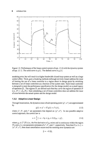
requirements. This example further considers Example 2.1 to motivate additional
issues related to the adaptive function approximation problem.
Let f be a polynomial of order m. Then, one possible choice of a basis for this
approximator is (see Section 3.2) $(z) = [l,
z, ...,PIT.Figure 2.5 displays the
function approximation results foronesetofexperimental data (600samples)and four
different order polynomials. The x-axis of this figure corresponds to D = [-T, T ]
as specified in Example 2.1. Each of the polynomial approximations fits the data in
the weighted least squares sense over the range of the data, which is approximately
B = (-2; 2). Outside of the region B,the behavior of each approximation is distinct.
The disparity of the behavior of the approximators on D - B should motivate
questions related to the idea of generalization relative to the training data. First, we
dichotomize the problem into local and nonlocal generalization. Gocalgeneralization
refers to the ability of the approximator to accurately compute f(x) = f ( z ,+dz)
where z, is the nearest training point and dz is small. Local generalization is a neces-
sary and desirable characteristic of parametric approximators. Local generalization
allows accurate function approximation with finite memory approximators and finite
amounts of training data. The approximation and local generalization characteristics
of an approximator will depend on the type and magnitude of the measurement noise
and disturbances, the continuity characteristics off and f,and the type and number
of elements in the regressor vector 4. NFnlocal generalization refers to the ability of
an approximatorto accuratelycompute f(x)for z E V - B.Nonlocal generalization
is always a somewhat risky proposition.
Although the designer would like to minimize the norm of the function approxima-
tion errors, l/f(z)-f(z)//dz,
this quantity is not able to be evaluated online, since
f ( z )is not known. The norm ofthe sample data fiterror C,"=,
lIyz-f(z,)11can be
evaluated and minimized. Figure 2.6 compares the minimum of these two quantities](https://image.slidesharecdn.com/adaptive-approximation-based-controlcompress-230219164415-f6eb4a64/85/adaptive-approximation-based-control_compress-pdf-54-320.jpg)
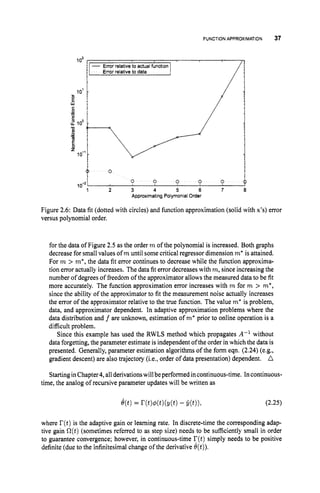
![38 APPROXIMATION THEORY
1 EXAMPLE2.5
The continuous-time least squares problem estimates the vector 0 such that $(t)=
$(t)Te minimizes
J(0)= ( y ( 7 )- G ( T ) ) ~
d7 = ( y ( 7 )- 4(7)T@)2
d7 (2.26)
1' 1'
where y : X+H X
'
,0 E XN,and q5 : X+H XN.Setting the gradient of J(0)with
respect to 0 to zero yields the following
1'4(7)(Y(7)- 4(4'0) d r = 0
I'$(T)Y(T)d.T = Lt@ ( 4 4 ( 4 T d T0
R(t) = P-'(t) 0
e(t) = P(t)R(t) (2.27)
where R(t)=
tions of P and R, that P-' is symmetric and that
@(.r)y(r)dTand P-l(t) =
d
dt
(b(7)4(T)'d.. Note by the defini-
- R t ) l = #(t)y(t)
Since P(t)P-l(t)= I , differentiation and rearrangement shows that in general the
time derivative of a matrix and its inverse must satisfy P = -P$ [P-'(t)]P;
therefore, in least squares estimation
P = -P(t)$(t)q(t)TP(t). (2.28)
Finally, to show that the continuous-time least squares estimate of 0 satisfies eqn.
(2.25) we differentiate both sides of eqn. (2.27):
e(t) = P(t)R(t)
+P(t)&(t)
= -P(t)~(t)@(t)TP(t)R(t)
+P(t)dt)Y(t)
= P(t)4(t)(-4WTW) +!At))
d(t) = W d t ) (Y(4 -B(t)). (2.29)
Implementation of the continuous-time least squares estimation algorithm uses equa-
tions (2.28)-(2.29). Typically,the initial value of the matrix P is selected to be large.
The initial matrix must be nonsingular. Often, it is initialized as P(0)= y I where y
n
is a large positive number. The implementation does not invert any matrix.
Before concluding this section, we consider the problem of approximating a function
over a compact region V.The cost function of interest is
(.m- ~ ( z ) ~ e ) ~
(M - q 5 ~ ~ 0 )
d z .](https://image.slidesharecdn.com/adaptive-approximation-based-controlcompress-230219164415-f6eb4a64/85/adaptive-approximation-based-control_compress-pdf-56-320.jpg)
![APPROXIMATORPROPERTIES 39
Again, we find the gradient of J with respect to 8, set it to zero, and find the resulting
parameter estimate. The final result is that 8must satisfy (see Exercise 2.9)
(2.30)
Computation of 8by eqn. (2.30) requires knowledge of the function f. For the applications
of interest herein, we do not have this luxury. Instead, we will have measurements that
are indirectly related to the unknown function. Nonetheless, eqn. (2.30) shows that the
condition of the matrix s
, 4 ( ~ ) 4 ( z ) ~ d z
is important. When the elements of the 4 are
mutually orthonormal over D,then s
, $ ( ~ ) $ ( z ) ~ d z
is an identity matrix. This is the
optimal situation for solution of eqn. (2.30), but is often not practical in applications.
2.4 APPROXIMATOR PROPERTIES
This section discusses properties that families of function approximators may have. In
each subsection, the technical meaning of each property is presented and the relevance and
tradeoffs of the property in the applications of interest are discussed. Due to the technical
nature of and the broad background that would be required for the proofs, in most cases the
proofs are not presented. Literature sources for the proofs are cited.
2.4.1 Parameter(Non)Linearity
An initial decision that the designer must make is the form of the function approximator. A
large class of function approximators (several arepresented in Chapter 3)canbe represented
as
f^(z: 8,.
) = eT+, g) (2.31)
where z E En,8 E !RN,and the dimension of u depends on the approximator of interest.
The approximator has a linear dependence on 8,but a nonlinear dependence on u.
rn EXAMPLE2.6
The (N-I)-th order polynomial approximation f^(z: 8,N)= CE-' 8,zifor z E $3'
has the form of eqn. (2.31) where $(z,N) = [ l , ~ ,
...,zN-']'. If N is fixed,
then the polynomial approximation is linear in its adjustable parameter vector 8 =
[&,...,ON-']. See Section 3.2 for amoredetailed discussionofpolynomialapprox-
imators. n
rn EXAMPLE2.7
The radial basis function approximator with Gaussian nodes:
with z, ci E !Rn and &, 7, E !R1, has the form of eqn. (2.31) where](https://image.slidesharecdn.com/adaptive-approximation-based-controlcompress-230219164415-f6eb4a64/85/adaptive-approximation-based-control_compress-pdf-57-320.jpg)
![40 APPROXIMATIONTHEORY
and
This radial basis function approximator is only linear in its parameters when all
elements of a are fixed, See Section 3.4for amore detailed discussion of radial basis
function approximators. a
W EXAMPLE23
The sigmoidal neural network approximator
N
f
^
(
.
:8,a))= c8ig(XTZ +bz)
i-I
with nodalprocessingJirnctiong defined by the squashing function g(u) = -has
the form of eqn. (2.31) where
and
f
J= [XI,. .., X N , b l , . .., b N ] .
The sigmoidal neural network approximator is again linear in its parameters if all
elements of the vector u are fixed apriori. Sigmoidal neural networks are discussed
in detail in Section 3.6. n
In most articles and applications, the parameter N which is the dimension of 4 is fixed
prior to online usage of the approximator. When N is fixed prior to online operation,
selection of its value should be carefully considered as N is one of the key parameters that
determines the minimum approximation accuracy that can be achieved. All the uniform
approximation results of Section 2.4.5 will contain a phrase to the effect “for N sufficiently
large.” Self-organizing approximators that adjust N online while ensuring stability of the
closed-loop control system constitute an area of continuing research.
A second key design decision is whether a will be fixed apriori (i.e., a(t)= a(0)and
u = 0)or adapted online (Le., a(t)is a functionoftheonline data and controlperformance).
If0isfixedduring onlineoperation,then the hnction approximator is linear intheremaining
adjustable parameters 8 so that the designer has a linear-in-the-parameter (LIP) adaptive
function approximation problem. Proving theoretical issues, such as closed-loop system
stability, is easier in the LIP case. In the case where the approximating parameters a are
fixed, these parameters will be dropped from the approximation notation, yielding
j(5)= 8T$(z). (2.32)
Fixing u is beneficial in terms of simplifying the analysis and online computations, but may
limit the functions that can be accurately approximated and may require that N = dim($)
be larger than would be required if 0 were estimated online.
Example 2.8 has introduced the term nodalprocessingfinction. This terminology is
used when each node in a network approximator uses the same function, but different](https://image.slidesharecdn.com/adaptive-approximation-based-controlcompress-230219164415-f6eb4a64/85/adaptive-approximation-based-control_compress-pdf-58-320.jpg)
![APPROXIMATORPROPERTIES 41
nonlinear parameters. In Example 2.8, the i-th component of the $ can be written as
$
i
(
z
)= g(z : Xi, bi). Using the idea of a nodal processor, the i-th element of the regressor
vector in Example 2.7 can be written as 4
i
(
z
)= g(z : ci,ri)where for that example the
nodal processor is g(u) = e z p (-u2)).Many ofthe other approximators defined in Chapter
3 can be written using the nodal processor notation.
To obtain a linear in the parameters function approximation problem, the designer must
specify apriori values for (n,
N ,9,u). If these parameters are not specified judiciously,
then an approximator achieving a desired €-accuracy may not be achievable for any value
of 8. After (n,
N ,9,u) are fixed, a family of linear in the parameter approximators results.
Definition 2.4.1 (Linear-in-Parameter Approximators) Thefamily ofn input, N node,
LIP approximatorsassociated with nodalprocessor g(.) is dejned by
(2.33)
}
N
s ~ , N , ~ , ~
= f : R%+ 8' f(z)= C~ i $ i
(z) = eT$(z)
{ I i=l
with
This family of LIP approximators defines a linear subspace of functions from 92%to 9'. A
basis for this linear subspace is {$i ( z ) } ~ = ~ .
The relative drawbacks of approximators that are linear in the adjustable parameters
are discussed, for example, by Barron in [17]. Barron shows that under certain technical
assumptions, approximators that are nonlinear in their parameters have squared approxima-
tion errors of order 0 ($)while approximators that are linear in their parameters cannot
have squared approximation errors smaller than order 0 (h)
(N is the number of nodal
functions, n is the dimension of domain 2)). Therefore, for n > 2 the approximation error
for nonlinear in the parameter families of approximators can be significantly less than that
for LIP approximators. This order of approximation advantage for nonlinear in the parame-
ter approximators requires significant tradeoffs, that will be summarized at the end of this
subsection. Note that this order of approximation advantage is a theoretical result, it does
not provide a means of determining approximator parameters or an approximator structure
that achieves the bound.
A cost function Je(e)is strictly convex in e if for 0 5 (Y 5 1and for all e l ,e2 E El, the
function J, satisfies
E En, and 8 E ENwhere $i (z) = g(z : ui) and ui isfied at the design stage.
N
If a continuous strictly convex function has a minimum e*,then that minimum is a unique
global minimum.
If J, is strictly convex in e and e ( z ) = eT$(z), then for an fixed value z
ithe cost
function J(8) = Je(eT$(zi))
is only convex in 8. This is important since some of the
parameter estimation algorithmsto be presented in Chapter 4 will be extensions of gradient
following methods. For discussion, let e = $(zi)T8 where $(xi) is a constant vector.
Then, there is a linear space of parameter vectors Oi such that e
' = $(zi)T8, V6 E Qi.
The fact that J is strictly convex in e and convex in 8 for LIP approximators ensures that
for any initial value of 8, gradient based parameter estimation will cause the parameter
estimate to converge toward the space Oi (i.e., for LIP approximators, although there is a
linear space of minima, there is a single basin of attraction). Alternatively when J,(e) is
convex but the approximator is not linear in its parameters (i.e., j ( z ,6,a) = BT$(z,a
)
)
,
then the cost function J(8,u ) = J,(eT$(z, u))may not be convex in 6and u. If the cost](https://image.slidesharecdn.com/adaptive-approximation-based-controlcompress-230219164415-f6eb4a64/85/adaptive-approximation-based-control_compress-pdf-59-320.jpg)
![APPROXIMATOR PROPERTIES 43
putation of the approximator is also significantly reduced, see Section 2.4.8.4. Additional
advantages of LIP approximators are simplification of theoretical analysis, the existence of
a global minimizing parameter value, the ability toprove global (in the parameter estimate)
convergence results, and the ability (if desired) to initialize the approximation parameters
based on prior data or model information using the methods of Section 2.3. An additional
motivation for the use of LIP approximators is discussed in Section 2.4.6.
In the batch training of LIP approximators by the least squares methods of Section
2.3.1, unique determination of 0 is possible once @ is nonsingular. In the literature, this
is sometimes referred to as a guaranteed learning algorithm [31]. This is in contrast to
gradient descent learning algorithms (especially in the case of non-LIP approximators) that
(possibly) converge asymptotically to the optimal parameter estimate.
2.4.2 Classical Approximation Results
This section reviews results from the classic theory of function approximation [155, 2181
that will recur in later sections and that have direct relevance to the stated motivations
for using certain classes of function approximators. The notation and technical concepts
required to discuss these results will be introduced in this section and used throughout the
reminder of the text.
2.4.2.I BackgroundandNotation The set of functions3 ( D )definedon a compact
set4 2)is a linear space (i.e., iff, g E F,then cuf +pg E F.).
The m-norm of F(D)is
defined as
llflloc = SUP If(.)l.
X E D
The set C(D)of continuous functions definedon D is also a linear space of functions. Since
D is ~ompact,~
for f E C(D),
Since supzEDIf(z)l satisfies the properties of a norm, both F(D)
and C(D)are normed
linear spaces. Given a norm on F(D),
the distance between f,g E F(D)
can be defined as
d(f,
g) = Ilf -g1/.When f,g are elements of a space S,d(f,g) is a metric for S and the
pair {S,d } is referred to as a metric space. When S(D)is a subset of F(D),the distance
from f E F(D)
to S(D)is defined to be d(f,S) = infaESd(f,a).
A sequence {fi} E X is a Cauchysequence if ilfi -fj 11 + 0as i,j -+ 00. A space X is
complete if every Cauchy sequence in X converges to an element of X (i.e., ilfi - fll ---t 0
as i -+ m for some f E X ) . A Banach space is the name given to a complete normed
linear space. Examples of Banach spaces include the C
, spaces for p 1 1where
or the set C(D)with norm ilfliw.
4Thefollowingpropertiesareequivalentforafinitedimensionalcompactset '
D c X:(1) V isclosedandbounded,
(2) every infinite cover of V has a finite subcover (i.e.,Given any {di}c,
c K such that '
D C Uzld,, then
there exist N such that V C U z N d i ) ,
(3) every infinite sequence in V has a convergentsubsequence.
51ff is a continuous real function defined over a compact region V,then f achieves both a maximum and a
minimum value on V.](https://image.slidesharecdn.com/adaptive-approximation-based-controlcompress-230219164415-f6eb4a64/85/adaptive-approximation-based-control_compress-pdf-61-320.jpg)
![44 APPROXIMATIONTHEORY
EXAMPLE2.9
Let D = [0,1].Is C(D)
with the C2 norm complete?
Consider the sequence of functions { z ~ } ? ? ~
each of which is in C(D).
Basic
calculus and algebra (assuming without loss of generality that m > n)leads to the
bound
Since the right-hand side can be made arbitrarily small by choice on n,{s”}?=~is a
Cauchy sequence of function in C(D)
with norm 11 . 112. The limit of this sequence is
the function
which is not in C(D).
Therefore, by counterexample, C(D)
with the C
z norm is not
complete.
n
Note that this sequence is not Cauchy with the m-norm.
2.4.2.2 WeiersfrassResults Given a Banach space K with elements f,norm ilfii,
and a sequence @N= {@i}zl
C X of basis elements, f is said to be approximable by
linear combinations of @N with respect to the norm 11 . /Iif for each E > 0 there exists N
such that ilf - P~11< E where
N
P N ( z ) = Cei4&), for some ~i E R. (2.34)
i=l
The N-th degree o
f approximation off by @N is
E:(f) = d(f, P N ) = i
!
f 1
I
.
f - p N i / .
Whenthe infimum is attained forsomeP E K ,this Pisreferred to as the linear combination
of best approximation.
Consider the theoretical problem of approximating a given function f E C(D)relative
to the two norm using PN.The solution to eqn. (2.30) is
(2.35)
where the basis elements @i (x)are assumed to be linearly independent so that
is not singular.6 This solution shows that there is a unique set of coefficients for each N
such that the two-norm of the approximation error is minimized by a linear combination of
the basis vectors. This solution does not show that f E C(D)
is “approximable by linear
combinations of @N,” since eqn. (2.35) does not show whether E $ ( f )approaches zero as
N increases.
6Notethe similarity between eqns. (2.13) and (2.35). The properties of the matrix to be inverted in the latter
equation are determined by V and the definitionof the basis elements. The properties of the matrix to be inverted
in the former equation depend on these same factors as will as the distribution of the samples used to define the
matrix.](https://image.slidesharecdn.com/adaptive-approximation-based-controlcompress-230219164415-f6eb4a64/85/adaptive-approximation-based-control_compress-pdf-62-320.jpg)
![APPROXIMATOR PROPERTIES 45
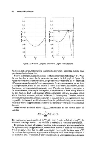
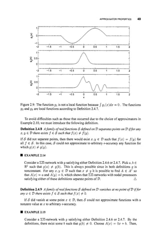
EXAMPLE 2.10
Let x ( x : a:b) be the characteristic function on the interval [u,b]:
1
0 otherwise.
for z E [u,b],
x ( x ,a, b) =
If the designer selects the approximator basis elements to be $i(x) = x ( x : 0,+)
where V = [O, 11,then
This matrix is nonsingular for all N . Therefore, for any continuous function f on V,
there exists a optimal set ofparameters given by eqn. (2.35) such that ELl
&$Ji(x)
achieves E:(f). However, this choice of basis function, even as N increases to
infinity,cannot accurately approximate continuous functions that are nonconstant for
.A
x E [0.5,I](e.g., f(x)= 2).
The previous example shows that for a set of basis elements to be capable of uniform
approximation of continuous functions over a compact region V,
conditions in addition to
linear independence of the basis elements over V must be satisfied. The uniform approxi-
mation property of univariate polynomials
1
N
pN(x)= akXk,x ,arc E 8
'
{k
=
O
is addressed by the Weierstrass theorem.
Theorem 2.4.1 Each realfinctionf that is continuous on D = [u,b] is approximable by
algebraicpolynomials with respect to the co-norm: VE> 0, 3M such that ifN > M there
exists apolynomial p E PN with Ilf(x)-p(x)lloc< Efor all x E D.
A set S being dense on a set 7means that for any E > 0 and T E 7,there exists S E S
such that 1
1
s- TI1 < E. A simple example is the set of rational numbers being dense on
the set of real numbers. The Weierstrass theorem can be summarized by the statement that
the linear space of polynomials is dense on the set of functions continuous on compact D.
It is important to note that the Weierstass theorem shows existence, but is not constructive
in the sense that it does not specify M or the parameters [uo,...,U M ] .
EXAMPLE 2.11
The Weierstrass theorem requires that the domain D be compact. This example
motivates the necessity of this condition.
Let D = (0,1], which is not compact. Let f = i,
which is continuous on D.
Therefore, all preconditions of the Weierstrass theorem are met except for D being
compact. Due to the lack of boundedness off on D and the fact that the value of any](https://image.slidesharecdn.com/adaptive-approximation-based-controlcompress-230219164415-f6eb4a64/85/adaptive-approximation-based-control_compress-pdf-63-320.jpg)
![46 APPROXIMATIONTHEORY
element of PNas x + 0 is a0 < 00, E accuracy over D cannot be achieved no matter
n
how large N is selected.
The remainder of this chapter will introduce the concept of network approximators and
discuss the extension of the above approximation concepts to network approximators.
2.4.3 Network Approximators
Network approximators included some traditional (e.g., spline) and many recently intro-
duced (e.g., wavelets, radial basis functions, sigmoidal neural networks) function approxi-
mation methods. Thebasic idea of anetwork approximator istouse apossibly large number
of simple, identical, interconnected nodal processors. Because of the structure that results,
matrix analysis methods are natural and parallel computation is possible.
Consider the family of affine functions.
Definition 2.4.2 (Affine Functions) For any T E {1,2,3...}, A' : 8
' + 8' denotes the
set of affine functions of theform
A(x) = wTx +b
where w,x E 8
' and b E 8',
Theaffinefunction A(x)definesahyperplane that divides 8
' into two sets {x E 8
' IA(x) 1
0 ) and {x E R'lA(x) < O}. In pattern recognition and classification applications, such
hyperplane divisions can be used to subdivide an input space into classes of inputs [152].
Network approximators are defined by constructing linear combinations of processed
affine functions [259].
Definition 2.4.3 (Single Hidden Layer (C) Networks) Thefamily of r input, N node,
single hidden layer (E) network approximators associated with nodal processor g(.) i
s
defined by
where@=[el;...,ON].
The C designation in the title of this definition indicates that each nodal processor sums
its scalar input variables. The type of nodal processor selected determines the form of the
nodal processor g(.). In network function approximation structures x is the network input,
w are the hidden layer weights, b is a bias, and @ are the output layer weights.
EXAMPLE 2.12
The well-known single-layer perceptron (which will be defined later in Section 3.6)
is a C network there Ai would denote the input layer parameters of the i-th neuron.
n
Extending the C-network definition to allow nodal processors with outputs that are the
product of C-networkhidden layer outputsproduces awider class ofnetworkapproximators.](https://image.slidesharecdn.com/adaptive-approximation-based-controlcompress-230219164415-f6eb4a64/85/adaptive-approximation-based-control_compress-pdf-64-320.jpg)
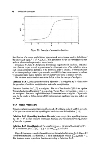
![50 APPROXIMATIONTHEORY
g(A(z))
# 0. Therefore, ZIT-networks with nodal processors satisfying either of
n
these definitions satisfy Definition 2.4.9.
2.4.5 UniversalApproximator
Consider the following theorem.
Theorem 2.4.2 Given f E C2('D)and an approximator of theform eqn. (2.32),for any
N i j (s, @~(z)@L(z)dz)
is nonsingulal; then there exists a unique 0* E !RN such that
f(z)
= (19*)~4(s)
+e'j(z) where
(2.36)
In addition, there are no local minima of the costfunction (other than 0*).
This theorem states the condition necessary that for a given N , there exists a unique para-
meter vector 0* that minimizes the C2 error over 2). In spite of this, for f € &(D), the
error e;(z) may be unbounded pointwise (see Exercise 2.7). Since V is compact, iff and
@N E C(2)),then e;(z) is uniformily bounded on 2
)
,but the theorem does not indicate
how e;(z) changes as N increases. This is in contrast to results like the Weierstass theorem
which showed polynomials could achieve arbitrary €-accuracyapproximation to continuous
functionsuniformly over a compact region, if the order of the polynomial was large enough.
Development of results analogous to the Weierstrass theorem for more general classes of
functions is the goal of this section.
For approximation based control applications, a fundamental question is whether a par-
ticular family of approximators is capable ofprovidinga close approximation to the function
f(x).There are at least three interesting aspects of this question:
1. Is there some subset of a family of approximators that is capable of providing an
e-accurate approximation to f(x)uniformly over D.
2. If there exists some subset of the family of approximators that is capable of providing
an e-accurate approximation, can the designer specify an approximation structure in
this subset apriori?
3. Given that an approximation structure can be specified, can appropriate parameter
vectors 6
'and o be estimated using data obtained during online system operation,
while ensuring stable operation?
The first item is addressed by the universal approximation results of this subsection. The
second item is largely unanswered, but easier for some approximation structures. Item 2 is
discussed in Chapter 3. Item 3 which is a main focus of this text is discussed in Chapters
4-7. The discussion of this section focuses on single hidden layer networks. Similar results
apply to multi-hidden layer networks [88,259].
The N-th degree of approximation off by S r , ~
is](https://image.slidesharecdn.com/adaptive-approximation-based-controlcompress-230219164415-f6eb4a64/85/adaptive-approximation-based-control_compress-pdf-68-320.jpg)
![APPROXIMATOR PROPERTIES 51
Uniform Approximation is concerned with the question ofwhether for aparticular family of
approximators and f having certain properties (e.g., continuity), is it guaranteed to be true
that for any E > 0, E$ (f)< E if N is large enough? Many such universal approximation
results have been published (e.g.,[58, 88, 110, 146, 193,2591). This section will present
and prove one very general result for Ell-networks [1lo], and discuss interpretations and
implications of this (and similar) results. Theorem 2.4.5 summarizes related results for
C-networks.
The proof for XI-networks uses the Stone-Weierstrass Theorem [48] which is stated
below.
Theorem 2.4.3 (Stone-Weierstrass Theorem) Let S be any algebra of real continuous
jimctions on a compact set D. rfS separates points on D and vanishes at nopoint of D,
thenfor any f E C(D)
and E > 0 there exists f E S such that supDif(.) - f(.)l < E.
Theorem 2.4.4 ([l lo]) Let 2)be a compact subset of !Rr and g : !R1 H !R1 be any con-
tinuous, nonconstantfunction. The set S of Ell-networks with nodalprocessors specified
by g has the property thatfor any f E C(D)
and E > 0 there exists f E S such that
SUPD If(.) - m< E.
Extensions of the examples of Section 2.4.4show that for any continuous nonconstant g,
CJI-networks satisfy the conditionsofthe Stone-Weierstrass Theorem. Therefore, the proof
of Theorem 2.4.4follows directly from the Stone-Weierstrass Theorem. An interesting and
powerful feature of his theorem is that g is arbitrary in the set of continuous, nonconstant
functions. The following theorem shows that C-networks with appropriate nodal functions
also have the universal approximation property. The proof is not included due to the scope
of the results that would be required to support it.
Theorem 2.4.5 r f g is either a squashingfunction or a localfunction (according to Deji-
nitions 2.4.6or 2.4.7respectively), f is continuous on the compact set D E !Rr, and S is
thefamily of approximators dejned as C network (according to Dejinition 2.4.3),thenfor
a given E there exist R(E)
such thatfor N > S(E)
there exist f^ E ST,^ such that
for an appropriately defined metric pforfunctions on D.
Approximators that satisfy theorems such as 2.4.4and 2.4.5 are referred to as universal
approximators. Universal Approximation Theorems suchas this statethat under reasonable
assumptionsonthenodalprocessor andthefunction tobe approximated, ifthe(single hidden
layer) network approximator has enough nodes, then an accurate network approximation
can be constructed by selection of 8 and u. Such theorems do not provide constructive
methods for determining appropriate values of N:8, or 0.
Universal approximation results are one of the most typically cited reasons for applying
neural or fuzzytechniques in control applications involvingsignificantunmodeled nonlinear
effects. The reasoning is along the following lines. The dynamics involve a function
f(x)= fo(x)+f*(x)where f*(x)has a significant efect on the system performance
and is known to have properties satisfiing a universal approximation theorem, but f * (x)
cannot be accurately modeled a priori. Based on universal approximation results, the
designer knows that there exists some subset of S that approximates f* (x)to an accuracy
Efor which the control specification can be achieved Therefore,the approximation based](https://image.slidesharecdn.com/adaptive-approximation-based-controlcompress-230219164415-f6eb4a64/85/adaptive-approximation-based-control_compress-pdf-69-320.jpg)
![52 APPROXIMATIONTHEORY
controlproblem reduces tofinding f E S that satisjies the E accuracy spec@ation. Most
articles in the literature address the third question stated at the beginning of this section:
selection of I9 or (0,o)given that the remaining parameters of S have been specified.
However, selection of N for a given choice of g and a (or ( N ,cr) for a specified g) is
the step in the design process that limits the approximation accuracy that can ultimately
be achieved. To cite universal approximation results as a motivation and then select N as
some arbitrary, small number are essentialiy contradictory.
Starting with the motivation stated in the previous paragraph, it is reasonable to derive
stable algorithms for adaptive estimation of I9 (or (8,a
)
) if N is specified large enough
that it can be assumed larger than the unknown 8.Specification of too small of a value
for N defeats the purpose of using a universal approximation based technique. When N is
selected too small but a provably stable parameter estimation algorithm isused, stable (even
satisfactory) control performance is still achievable; however, accurate approximation will
not be achievable. Unfortunately, the parameter m is typically unknown, since f*(x)is
not known. Therefore, the selection of N must be made overly large to ensure accurate
approximation. The tradeoff for over estimating the value of N is the larger memory and
computation time requirements of the implementation. In addition, if N is selected too
large, then the approximator will be capable of fitting the measurement noise as well as the
function. Fourier analysis based methods for selecting N are discussed in [232]. Online
adjustment of N is an interesting area of research which tries to minimize the computational
requirements while minimizing E and ensuring stability [13, 37,49, 72, 89, 1781.
Results such as Theorems 2.4.4and 2.4.5 provide sufficient conditions for the approxi-
mation of continuous functions over compact domains. Other approximation schemes exist
that do not satisfy the conditions of these particular theorems but are capable of achiev-
ing E approximation accuracy. For example, the Stone-Weierstrass Theorem shows this
property for polynomial series. In addition, some classical approximation methods can be
coerced into the form necessary to apply the universal approximation results. Therefore,
there exist numerous approximators capable of achieving E approximation accuracy when
a sufficiently large number of basis elements is used. The decision among them should be
made by considering other approximator properties and carefully weighing their relative
advantages and disadvantages.
2.4.6 Best Approximator Property
Universal approximation theorems of the type discussed in Section 2.4.5 analyze the prob-
lem of whether for a family of function approximators S r , ~ ,
there exists a E ST,^ that
approximates a given function with at most E error over a region D. Universal approxima-
tion results guarantee the existence of a sequence of approximators that achieve EL-accuracy,
where { E ~ }is a sequence that converges to zero. Depending on the properties of the set
S r , ~ ,
the limit point of such a sequence may or may not exist in S r , ~ .
This section considers an interesting related question: Given a convergent sequence of
approximators {ai}, ai E ST,^, is the limit point of the sequence in the set S
,
,
,
? If the
limit point is guaranteed to be in S r , ~ ,
then the family of approximators is said to have
the best approximator property. Therefore, where universal approximation results seek
approximators that satisfy a given accuracy requirement, best approximation results seek
optimal approximation accuracy.
The best approximation problem [97, 1551 can be stated as “Given f E C(D)and
Sr,N C C ( D ) ,find a
’ E ST,^ such that d(f,a*) = d(f.S?,N).’’A set S r , ~
is called an
existenceset if for any f E C(D)there is at least one best approximationto f in ST,,,. A set](https://image.slidesharecdn.com/adaptive-approximation-based-controlcompress-230219164415-f6eb4a64/85/adaptive-approximation-based-control_compress-pdf-70-320.jpg)
![APPROXIMATOR PROPERTIES 53
S,-..~,J is called a uniqueness set if for any f E C(D)there is at most one best approximation
to f in S,-,N.A set S r , ~
is called a Tchebychefset if it is both a uniqueness set and an
existence set. The results and discussion to follow are based on [48, 971.
Theorem 2.4.6 Every existence set is closed
Proof. Assume that existence set S c C(V)is not closed. Then there exists a convergent
sequence {si} c Ssuch that the limit f $Z S. Since f is a limit of {si},d(f,
S)= 0. Since
S is an existence set, there exists g E S such that d(f,g) = 0. This implies that f = g
which is a contradiction. Therefore, Smust be closed.
Theorem 2.4.7 IfA is a compact set in metric space (S,11 ti), then A is an existence set.
Proof. Let p = d(f.A) for f E S. By the definition of d as an infimum there exists
a sequence {a,} c A such that d(f,a,) converges to p as i + m. By the compactness
of A, the sequence {a,} has a limit a* E A. By the triangle inequality, d(f.a*) 5
d(f,a k ) +d(ak,a*).Since the left side is independent of k and the right side converges
to p, d(f.a*) 5 p. By the definition of p as the infimum over all elements of A, it is
necessary that d(f.a*)
2 p. Combining inequalities gives d(f.a*) = p, which shows that
the best approximation is achieved by an element of A.
The above two theorems show that a set being closed is a necessary, but not sufficient
condition for a set to be an existence set. Compactness is a sufficient condition.
Theorem 2.4.8 For g continuous and nonconstant, let Sn,~,g,,,
c C(V)be defined as in
Definition 2.4.1, then Sn,~,g,u
is an existence set.
Proof. Let f be an arbitrary fixed element of C(V).
Choose an arbitrary h E Sn,~.g,o.
The set
is closed and bounded. Therefore, the finite dimensional set 7 - l ~
is compact. Theorem
7 - t ~
= (9 6 Sn.N.g,a 1/19- fll 5 IIh- fll1
2.4.7 implies that 7-t (and therefore Sn,,v,g,a)
is an existence set.
The set 7 - t ~
being closed and bounded relies on the assumption that Sn,~,y,o
C C(V)
is defined by a finite dimensional LIP approximator. When the approximator f^ in not LIP,
the proof will not typically go through, since the set 7-1defined relative to
for x E En,0 E Xm and .Q E SNis not usually closed. In particular, [97] shows that radial
basis functions with adaptive centers and sigmoidal neural networks with an adaptive input
layer (or multiple adaptive layers) do not have the best approximator property.
Although thebest approximation property isamotivationtousing LIP approximators, the
motivation is not strong. If €-accuracy approximation is required for satisfactory control
performance and an approximator structure S,-,N,~
can be defined which is capable of
achieving d-accuracy for some E
' < E, then there exist a subset A of S,-,N,~
that achieves
the desired €-accuracy approximation. However, it may be quite difficult to specify the
required approximation structure and find an element of the subset A.](https://image.slidesharecdn.com/adaptive-approximation-based-controlcompress-230219164415-f6eb4a64/85/adaptive-approximation-based-control_compress-pdf-71-320.jpg)
![APPROXIMATORPROPERTIES 57
The set of global models is a strict subset of the set of local models. This is obvious,
since if there exists a set of parameters 8 satisfying Definition 2.4.11 for a particular
E, then this 0 also satisfies Definition 2.4.10for the same c at each xo E V.
To maintain accuracy over domain V,a local approximation structure can either adjust its
parameter vector, through time, as the operating point zo changes; or store its parameter
vector asa function ofthe operating point. Theformer approach is typical of adaptive control
methodologies while the latter approach is being motivated herein as learning control. The
latter approach can effectively construct a global approximation structure by connecting
several local approximating structures.
A main objective of this subsection is to appropriately piece together a (large) set of
local approximation structures to achieve a global approximation structure. The following
definition of the class of Basis-Influence Functions [16, 76, 85, 122, 1731 presents one
means of achieving this objective.
Definition 2.4.12 (Basis-Influence (BI) Functions) - A function approximator is of the BI
Class ifand only ifit can be written as
(2.40)
i
where each fi(z,6) is a local approximation to f(z)
for all z E B(xi,6), and ri(x)has
local support S
iwhich is a subset of B(xi;6) such that D & uiSi.
Examples ofBasis-Influence approximators include: Boxes [23I], CMAC [2], Radial Basis
Functions [205], splines, and severalversions of fuzzy systems [198,2831. In the traditional
implementation of each of these approximators, the basis functions are constant on the
support of the influence function. If more capable basis functions (e.g., linear functions)
were implemented, then the designer should expect there to be a decrease in the number of
required local approximation structures. An alternative definition of local influence, which
also provides a measure of the degree of localization based on the learning algorithm, is
given in [288].
The partition of unity is defined as follows [253, 2931.
Definition 2.4.13 (Partition of Unity) - Theset ofpositive semidejnite influencefunctions
{ri}forma Partition ofunity on iffor any 5 E V ,
Influence functions that form a partition of unity have a variety of benefits. First, if {ri}
form a Partition of Unity on 'D, then there cannot be any x E V such that xgll?i(x)= 0.
Also, when the approximator is defined by eqn. (2.40) with {Ti} forming a Partition of
Unity, then at any z E 2
7
,f ( x ,6) is a convex combination of fi(z,6).
If a set of positive semidefinite influence functions {ri}do not form a partition of unity,
but have the coverage property (i.e., for any x E V there exists at least one i such that
Fi(x)# 0), then a partition of unity can be formed from {Ti}as
ri(x)= 1.
(2.41)
Thisnormalization operation should howeverbe used cautiously [2211. Suchnormalization
can yield ri(z)that have large flat areas. In addition, even when (x)is unimodal, I'i(z)
may be multimodal. See Exercise 2.10. When the functions T
i
(
.
) are fixedafter the design](https://image.slidesharecdn.com/adaptive-approximation-based-controlcompress-230219164415-f6eb4a64/85/adaptive-approximation-based-control_compress-pdf-75-320.jpg)
![APPROXIMATOR PROPERTIES 59
a EXAMPLE 2.17
A one input approximator that meets all the conditions of Theorem 2.4.9is
(2.44)
where xi = a$
and fi(x,8)can be any function capable of providing a local approximation to f(x)
at xi. n
a EXAMPLE 2.18
Figure 2.10 illustrates basis-influence function approximation. The routine for con-
structing this plot used r as defined in eqn. (2.45) with X = 0.785. In the notation
of Definition 2.4.12,for i = 1,... ,6:
where cz = 0.2(i - 1)and D = [0,1]. For clarity, the influence functions are plotted
at a 10%scale and only a portion of each linear approximation is plotted.
Note that the parameters of the approximator havebeenjointly optimized such that
eqn. (2.44) has minimum least squares approximation error over D.This does not
imply that each fi is least squares optimal over Si. This is clearly evident from the
figure. For example, f5 is not least squares optimal over S5 = [0.6,1.0].
The least
squared error of f5 over 5’5 would be decreased by shifting f5 down. It is possible to
improvethe local accuracy ofeach fi over Si,but this will increase the approximation
error of eqn. (2.44) over D. Often, this increase is small and such receptive field
weighted regression methods have other advantages in terms of computation and ap-
proximator structure adaptation (i.e., approximator self-organization) [13,236,2371.
n
2.4.8.2 Retention of TrainingExperience Based on the discussion of Subsection
2.4.7,the designer should not expect fto accurately extrapolate training data from regions
of D containing significant training data into other (unexplored) regions. In addition, it is
desirable for training data in new regions to not affect the previously achieved approxima-
tion accuracy in distant regions. These two issues are tightly interrelated. The issues of
localization and interference in learning algorithmswere rigorously examined in [288,289].
The online parameter estimation algorithms of Chapters 4, 6, and 7 will adapt the pa-
rameter vector estimate @(t)
based on the current (possibly filtered) tracking error e(t).
The algorithms will have the generic forms of eqns. (2.24) and (2.25).*If the regressor
(i.e., @(z))
has global support, then changing the estimated parameter 0, affects the ap-
proximation accuracy throughout D. Alternatively, if q& has local support, then changing
the estimated parameter Bt affects the approximation accuracy only on Suppm, which by
assumption is a small region of D containing the training point.](https://image.slidesharecdn.com/adaptive-approximation-based-controlcompress-230219164415-f6eb4a64/85/adaptive-approximation-based-control_compress-pdf-77-320.jpg)
![60 APPROXIMATIONTHEORY
-
$ 0 5 -
0 4 -
0 3 -
0 2
0 1
0.6
Figure 2.10: Basis-Influence Function Approximation of Example 2.18. The original func-
tion is shown as a dashed line. The local approximations (basis functions) are shown as
solid lines. The influence functions (drawn at 10% scale) are shown as solid lines at the
bottom of the figure.
EXAMPLE 2
.
1
9
Consider the task of estimating a function f
(
z
)
by an approximator f(z)=
As in a control application, assume that samples are obtained incrementally and the
z k f l is near x k . This example considers how the support characteristics of the basis
elements {r+f~i}& affects the convergence of the function approximation.
For computational purposes, assumethat f
(
z
)
= sin(z)andthe domain ofapprox-
imation D = [-T, 7r]. Also, let x k = -3.6 +0.lk for k = 0, .. .,72. Consider two
possible basis sets. The first set of basis elements is the first eight Legendre polyno-
mials (see Section 3.2) with the input to the polynomial scaled so that 'D H [-1,1].
This basis sets has global support over 'D. The approximator with the first eight
Legendre polynomials as basis elements is capable of approximating the sin func-
tion with a maximum error over '
D of approximately 1.0 x The second set
of basis elements is a set of Gaussian radial basis elements (see Section 3.4) with
centers at ci = -4 +0.52 for i = 0,...,16and spread = 0.5. Although each
Gaussian basis element is nonzero over all of D,each basis element is effectively
locally supported. This 17-element RBF approximator is capable of approximating
the sin function with maximum error over 'D of approximately 0.5 x low3.For both
approximators, initially the parameter estimate is the zero vector.
Figure 2.11 shows the results of gradient descent based (normalized least mean
squares) estimation of the sin function with each of the two approximators. The
Legendre polynomial approximation process is illustrated in the top graph. The RBF
approximation process is illustrated in the bottom graph. Each of the graphs contains
threecurves. The solidlineindicatesthe function f(z)that istobe approximated. The](https://image.slidesharecdn.com/adaptive-approximation-based-controlcompress-230219164415-f6eb4a64/85/adaptive-approximation-based-control_compress-pdf-78-320.jpg)
![APPROXIMATORPROPERTIES 61
A
B
- sin(x)
Trainingover [-3.4,-0 7
1
1H- - Trainingover [-3.4, 2.31 - ----- - - 1
_ _ - - - _
I I
Figure 2.11: Incremental Approximations to a sin function. Top - Approximation by
8-th order Legendre Polynomials. Bottom - Approximation by normalized Radial Basis
Functions. The asterisks indicate the rightmost training point for the two training periods
discussed in the text.
dotted line is the approximation at k = 29. At this time, the approximation process
has only incorporated training examples over the region V29 = [-3.6, -0.71. The
left asterisk on the x-axis indicates the largest value of x in D29. Note that both
approximators have partially converged over V29. The RBF approximation is more
accurate over V2g. Thepolynomial approximation has changed onV-V29. The RBF
approximation islargely unchanged on V-V29. The dashed line isthe approximation
at k = 59. At this time, theapproximation process has incorporated training examples
overtheregionD29 = [-3.6,2.3]. Therightasteriskonthex-axis indicates thelargest
value of x in 2759. Note that while the polynomial approximation is now accurate near
the current training point (z = 2.3), the approximation error has increased, relative
to the dotted curve, on V29. Alternatively,the RBF approximator is not only accurate
in the vicinity of the current training point, but is still accurate on V - V29, even
though no recent training data has been in that set. For both approximators, the norm
of the parameter error is decreasing throughout the training.
This example has used polynomials and Gaussian RBFs for computational pur-
poses, but the main idea can be more broadly stated. When the approximator uses
locally supportedbasis elements, there is a close correspondence between parameters
of the approximation and regions of V.Therefore, the function can be adapted lo-
cally to learn new information, without affecting the function approximation in other
regions of the domain of approximation. This fact facilitates the retention of past
training data. When the basis elements have global support, retention of past training](https://image.slidesharecdn.com/adaptive-approximation-based-controlcompress-230219164415-f6eb4a64/85/adaptive-approximation-based-control_compress-pdf-79-320.jpg)
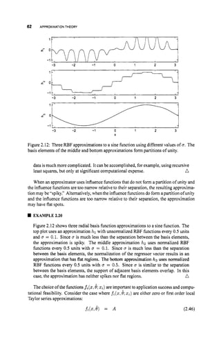
![APPROXIMATORPROPERTIES 63
or fi(z,
8) = A +B(Z- xi). (2.47)
In the first case, the basis functions are constants, as in the case of normalized radial
basis functions. For a given desired approximation accuracy E, many more basis-influence
pairs may be required if constant basis functions are used instead of linear basis functions.
Estimates of the magnitude of higher order derivatives can be used to estimate the number
of Basis Influence (BI) function pairs required in a given application.
The linear basis functions hold two advantages in control applications.
1. Linear approximations are often known a priori (e.g., from previous gain sched-
uled designs or operating point experiments). It is straightforward to use this prior
information to initialize the BI function parameters.
2. Linear approximations are often desired aposteriori either for analysis or design pur-
poses. These linear approximations are easily derived from the BI model parameters.
See the related discussion in Section 2.4.9of network transparency.
2.4.8.3 Curse of Dimensionality A well-known drawback [20]of function approx-
imators with locally supported regressor elements is the “curse of dimensionality,” which
refers to the fact that the number of parameters required for localized approximators grows
exponentially with the number of dimensions V.
EXAMPLE 2.21
Let d = dim(V).If V is partitioned into E divisions per dimension, then there will
n
be N = Edtotal partitions.
This exponential increase in N with d is a problem if either the computation time or
memory requirements of the approximator become too large. The embedding approach
discussed in Section 3.5 is a method of allowing the number of partitions of V to increase
exponentially without a corresponding increase in the number of approximator parameters.
The lattice networks discussed in Section 2.4.8.4illustrate a method by which the com-
putational requirements grow much slower than the exponential growth in the number of
parameters.
2.4.8.4 Lattice-BasedApproximators Specificationoflocally supportedbasis func-
tions requires specification of the type and support of each basis element. Typically, the
support of a basis element is parameterized by the center and width parameters of each $i.
This specification includes the choice as to whether the center and width parameters are
fixed apriori or estimated based on the acquired data.
Adaptive estimation ofthe center andwidth parameters isanonlinear estimationproblem.
Therefore, the resulting approximator would not have the best approximator property, but
would have the beneficial “order of approximation” behavior as discussed in Section 2.4.I.
Prior specification of the centers on a grid of points results in a lattice-based approxi-
mator [32]. Lattice-based approximators result in significant computational simplification
over adaptive center-based approximators for two reasons. First, the center adaptation cal-
culations are not required. Second, the non-zero elements of the vector q5 can be determined
without direct calculation of q5 (see below). If the width parameters are also fixed apriori,
then a linear parameter estimation problem results with the corresponding benefits.](https://image.slidesharecdn.com/adaptive-approximation-based-controlcompress-230219164415-f6eb4a64/85/adaptive-approximation-based-control_compress-pdf-81-320.jpg)
![64 APPROXIMATIONTHEORY
EXAMPLE 2.22
The purpose of this example [75] is to clarify how lattice-based approximators can
reduce the amount of computation required per iteration. For clarity, the example
discusses a two-dimensional region of approximation, as shown in Figure 2.13, but
the discussion directly extends to d > 2 dimensions.
AfunctionfistobeapproximatedovertheregionD= {(z)y) E [0,l]x[O,1
1
)
. If
the approximator takes the form f
(
z
)= OT#(z),where 6 E EN and q5 : R2-+ SRN,
then evaluationoff fora general approximatorrequires calculation ofthe N elements
of #
(
z
)followed by an N-vector multiply (with the associated memory accesses).
Assuming that $(z) ismaintained in memory between the approximator computation
and parameter adaptation, then adaptation of 8requires (at the minimum) a scalar by
N-vector multiply.
Alternatively, let the elements of #(z) be locally supported with fixed centers
defined on a lattice by
cm = C2,J = ((i - 1). dz, ( j - 1).dy)
for i = 1,...,nx
and j = 1,....ny,where N = n,ny, m = i +n, * ( j - l
)
,
dx = &, and dy = 1
n,-l. Also, let #z,3 (x) = g ((z,Y)-c ~ , ~ )
be locally
supported such g ((5,y) - c ~ , ~ )
= 0 if ii(z*y) - ljoo > A. The parameter X
is referred to as the generalization parameter. To allow explicit discussion in the
following, assume that X = 1.5dz. Also, as depicted in Figure 2.13, assume that
nz = ny= 5, so that dx = dy = 0.25. The figure indicates the nodal centers with
z’s and indicates the values of rnonthe lattice diagram. In general, these assumptions
imply that although N may be quite large, at most 9 elements of the vector I
$ will
X X I 8 x
l9 *OI
16 1 7
l3 x
X l 2 x
l4 ‘j:
11
6 7 * a 9 101
,x1
1 2 3 4 5
Figure 2.13: Lattice structure diagram for Example 2.22. The 2’s indicate locations of
nodal centers. The integers near the z’s indicate the nodal addresses m. The * indicates an
evaluation point.](https://image.slidesharecdn.com/adaptive-approximation-based-controlcompress-230219164415-f6eb4a64/85/adaptive-approximation-based-control_compress-pdf-82-320.jpg)
![66 APPROXIMATION THEORY
where fo(x)represents the known portion of the function and f*(x)represents the un-
known portion for which an approximation will be developed online. In this case, the
function approximator would approximate only f*(x).Second, if for some reason, the ap-
proach described in eqn. (2.48)is not satisfactory, then f(x)could be initialized by offline
methods to accurately approximate the known portion of the function (Lee,fo(x)).During
online operation, the parameters of the approximator would be tuned to account also for
the unknown portion of the function so that ultimately f(x)= fo(x)+f*(x).
Any approximator of the basis-influenceclass allows the user to interpret the approxi-
mated function. The influence functions dictate which of the basis functions are applicable
(and the amount of applicability) at any given point.
The fuzzy logic (see Section 3.7) interpretation of approximator transparency is slightly
more that the interpretation of the previous paragraph. In fuzzy logic approaches the
influence variables are often associated with linguistic variables: “small,” “medium,” or
“large.” Sothat the ideas of the previous paragraph together with the linguistic variable can
result in statements like: “If the ... is small, then use the control law ....” Similar ideas
could be extended to any lattice based approximator, but when the number of influence
functions per input dimension becomes large, the linguistic variables become awkward.
2.4.10 Haar Conditions
Section 2.2 introduced the idea of a Haar space: for unique function interpolation to be
possible by a LIP approximator with N basis elements using training data from an arbitrary
set of distinct locations {ai}L1,
the matrix @ = [q!~j(zi)]
must be nonsingular.
An example of a Haar subspace of Cia,b] is the set of N-dimensional polynomials
PN(z)defined on [a,b]. With the natural basis for polynomials, it can be shown that
I 1 1 ... 1 1
which is positive if it is assumed that the z
iare sorted such that 2
1 < xz < ... < ZN+I.
An N-dimensional Haar space (see Appendix A in [218]) can be considered as a gener-
alized polynomial in the sense that the Haar space is a linear space of functions that retains
the ability to interpolate a set of data defined at N arbitrary locations. For a Haar space
A c C[a,b],the following conditions are equivalent:
I. I f f E A and f is not identically zero, then the number of roots of the equation
2. Iff E A and fis not identically zero, if the number of roots of the equation f(z)
= 0
in [a,b] is j,and if k of these roots are interior points of [a,b] at which f does not
change sign, then (j+k) < N .
3. If { $ j , j = 1,...,N } is any basis for A, and if {zz,z= 1,...; N }is aset ofany N
distinct points in [a,b]then the N x N matrix [$J
(xi)]
is nonsingular.
The space PN of N-th order polynomials is an example of a Haar space. It is straightfor-
ward to show that spline functions (see Section 3.3) with fixed knots that are not dependent
on the data (or any approximator such that Supp(q5j)is finite) is not a Haar space. This is
f(z)= 0 in [a,b]is less than N .](https://image.slidesharecdn.com/adaptive-approximation-based-controlcompress-230219164415-f6eb4a64/85/adaptive-approximation-based-control_compress-pdf-84-320.jpg)
![APPROXIMATORPROPERTIES 67
shown using item 1 or item 3 of the Haar conditions as follows.
Item 1: Fix j as an integer in [I,N ] .Assume that Supp($j) c V,
Supp($j) # V ,and
This f^ is not identi-
v c uglSupp($i). Let f(x) = eT$(.) with ek =
cally zero, but has an infinite number of zeros since it is zero for all x E V - Supp($j).
Item 3: If { ~ i } ~ ~
is selected such that xi $2 Supp($j) for any i = 0,...,N , then the
matrix [#j(xi)]will have all zero elements in its j-th column. Therefore, this matrix is
singular.
The fact that approximators using basis elements with finite support do not generate
Haar spaces does not imply that such approximators are unsuitable for interpolation or
adaptive approximation problems. Instead, it implies that the choice of the points {xi}
affects the existence and uniqueness of a solution to the problem of interest. In offline data
interpolation problems, the points {xi} are used to define the center or knot locations of
the 4
j
,in such a way that the matrix [
4
j
(xi)]
is nonsingular.
In adaptive function approximation problems, defining the center or knot locations to
match the first N data locations is typically not suitable, since these data locations will
rarely be representative of all of V.At least three alternative approaches to the definition
of the center (or knot) locations are possible:
{
IC ' j
1 k = j .
1. A set of experimental data representative of all expected system operating conditions
could be accumulated and analyzed offline to determine appropriate center locations.
2. The center (or knot) locations could be altered during online operation as new data
is received.
3. The center (or knot) locations could be defined, possibly on a lattice, such that the
union of the support of the basis elements covers V.
None of these three approaches will ensure that the interpolation problem is solvable after
N samples, but that is not the objective. Instead, if appropriately implemented, these
approacheswill ensurethat accurate approximation ispossible over V.Parameter estimation
by the methods of Chapter 4 will result in convergence of the approximator locally in the
neighborhood of each sample point. Because the sample points cover all of V,global
convergence can be achieved.
Note that the Haar condition ensures that the matrix [&(xi)] is nonsingular for solution
of the interpolation problem. The Haar condition does not ensure that this matrix is well-
conditioned.
2.4.11 Multivariable Approximation by Tensor Products
Fordimensions greaterthan one, onemeansforconstructing basis functions is asthe product
ofbasis functionsdefined separateIyfor each dimension. This can be represented as atensor
product.
Let G = span(g1,. .., g p } (i.e., G = {gjg(x) = C;='=,
aigi(s),ai E @,gi : [a,b] ++
@}). Let H = span(h1 ...,hq}where hi : [c,d] ++ 9'. Then the tensorproduct of the
spaces G and H is](https://image.slidesharecdn.com/adaptive-approximation-based-controlcompress-230219164415-f6eb4a64/85/adaptive-approximation-based-control_compress-pdf-85-320.jpg)
![68 APPROXIMATIONTHEORY
where 4
; = [gl,...,gp],4: = [hl, ...,hp],and A = [aij].The function f canbe written
in standard LIP form with
eT = [all,...1 a1qr.. .,a p 1 , . .’ ,apq1
and
If q%gand O h are partitions of unity, then the q corresponding to their tensor product is
also also a partition of unity since
(2.50)
(2.51)
Assume that G and H vanish nowhere on their respective domains. If G separates
points in [a,b] and H separates points in [c,d], then it is straightforward to show that
4(z,y) separates points in [a,b] x [c,d]. Therefore, it is also straightforward to show
that if G and H each satisfy the preconditions of the Stone-Weierstrass theorem, then
the tensor product of G and H also satisfies the Stone-Weierstrass theorem. Therefore,
G, @ Hp(z:
y) = span{gi(z)hj(y), i = 1,.
..,plj = 1,...,q } is a family of uniform
approximators in C([a;b] x [c,d]).
This product of basis function approach can be directly extended to higher dimensions,
but results in an exponential growth in the number of basis functions with the dimension
of the domain of approximation. This approach is not restricted to locally supported basis
elements. Itcan forexamplebe applied topolynomial basis elementstoproduce multivariate
polynomials.
2.5 SUMMARY
This chapter has introduced various function approximation issues that are important for
adaptive approximation applications. In particular, this chapter has motivated why var-
ious issues should (or should not) be taken into account when selecting an appropriate
approximator for a particular application.
Since the number of training samples will eventually become large, approximation by
recursive parameter update eventually becomes important. All the data cannot be stored
and a basis function cannot be associated with each training point. Due to noise on the
measurements and the ever increasing number of samples, interpolation is neither desired
nor practical.
Severalfactors influencethe specification ofthe function approximator. Sincethe criteria
forafamilyof approximators tobecapableofuniform€-accuracyapproximation are actually
quite loose, the existence of uniform approximation theorems for a particular family of
approximators is not a key factor in the selection process. Important issues include the
memory requirements, the computation required per function evaluation, the computation
required for parameter update, and the numeric properties of the approximation problem.
These issues are affected by whether or not the approximator is LIP, has locally supported
basis elements, and is defined on a lattice. Various tradeoffs are possible.](https://image.slidesharecdn.com/adaptive-approximation-based-controlcompress-230219164415-f6eb4a64/85/adaptive-approximation-based-control_compress-pdf-86-320.jpg)
![EXERCISESAND DESIGNPROBLEMS 69
The concept of a partition of unity has also been introduced. Advantages of approxima-
tors having the partition of unity property are (1) such approximators vanish nowhere and
(2) such approximators are capable of exactly representing constant functions. The basis-
influence function idea has been introduced to group together a set of approaches involving
locally accurate approximations (i.e., basis functions) that are smoothly interpolated by the
influence functions to generate an approximator capableof accurate approximation over the
larger set V.Whenthe influence functions form a partition of unity, then the basis-influence
approximator is formed as the convex combination of the local approximations.
Once a family of approximators has been selected, the designer must still specify the
structure of the approximator, the parameter estimation algorithm, and the control archi-
tecture. Optimal selection of the structure of the approximator is currently an unanswered
research question. The designer must be careful to ensure that the approximation structure
that is specified is not too small or it will overly restrict the class of functions that can
ultimately be represented. The parameter N should also not be too large or the approxi-
mated function may fit the noise on the measured data. Parameter estimation algorithms
are discussed in Chapter 4. Control architectures and stability analysis are discussed in
Chapters 5 - 7.
2.6 EXERCISESAND DESIGN PROBLEMS
Exercise 2.1 Implement a simulation to duplicate the results of Section 2.1.
Exercise 2.2 Show that the parameter vector that jointly minimizes the norm of the para-
meter vector and the approximation error is 8 = ( X I +(PaT)-'(PY. Note that the cost
function for this optimization problem is
Exercise 2.3 Perform the matrix algebraic manipulations to validate the Matrix Inversion
Lemma.
Exercise 2.4 Show that if J ( e )is strictly convex in e and e is a linear function of 8, then
J is convex in 8.
Exercise 2.5 Derive eqn. (2.35).
Exercise 2.6 Following Definition 2.4.5 a series of statements is made about whether or
not given sets of functions are algebras. Prove each of these statements.
Exercise 2.7 Let f(z)= x-'I3 and V = [0,1].
1. Show that f E &(V).
2. Is f E C,(V)?
3. Use eqn. (2.35) to find the Cz optimal constant approximation (i.e., let $(x) = [l])
4. Use eqn. (2.35) to find the Cz optimal linear approximation (i.e., let 4(z) = [l,
zIT)
to f over V.
to f over V.](https://image.slidesharecdn.com/adaptive-approximation-based-controlcompress-230219164415-f6eb4a64/85/adaptive-approximation-based-control_compress-pdf-87-320.jpg)
![70 APPROXIMATIONTHEORY
For each of the constant and linear approximations, is the approximation error in &(D)?
.cm PP
Exercise 2.8 Repeat Example 2.l-using recursive weighted least squares to estimate the
parameters of the approximator f = eT@(z)
where $(z) is the Gaussian radial basis
function described in Example 2.19.
Exercise 2.9 Show that eqn. (2.30) is true.
Exercise 2.10 Thetext following Definition2.4.13discussed normalizationoftheinfluence
functions rito produce influence functions '
i
'
i forming a partition of unity. This problem
hrther considers the cautions expressed in that text. Let D = [0,I].
1. Let TI(z) = exp (- (:)') and l?z(z)= exp . Numerically computed
and plot {Fi(z)}i=1:2
and {ri(~)}i=~:2
over '
D with u = 1. Repeat for B = 0.1 and
u = 0.5. Discuss the tradeoffs involved with choosing u.
2. LetP1(z) = exp andfz(z) = exp (- (w)').
Plotanddiscussrl(z)
and rz(x).](https://image.slidesharecdn.com/adaptive-approximation-based-controlcompress-230219164415-f6eb4a64/85/adaptive-approximation-based-control_compress-pdf-88-320.jpg)

![72 APPROXIMATION STRUCTURES
M
Figure 3.1: Simple pendulum.
3.1 MODEL TYPES
This section discusses three approaches to adaptive approximation. The first subsection
discusses the use of a model structure derived from physical principles. The second subsec-
tion discusses the storage and use of the raw data without the intermediate step of function
approximation. The third section discusses the use of generic function approximators. It is
this third approach that will be the main focus of the majority of this text.
3.1.
I Physically Based Models
In some applications, the physics of the problem will provide a well-defined model struc-
ture where only parameters with well-defined physical interpretations are unknown. In
such cases, the physically defined model may provide a structure appropriate for adaptive
parameter identification.
EXAMPLE3.1
The dynamics of the simple pendulum of Figure 3.1 are
where T is the applied control torque. If the parameters A4 and L were unknown,
they could be estimated based on the model structure
where z = [$, 7
1
' and #(z) = [sin($), T ] ~ ,
while the parameters 8
1 and 82 are
defined as = f and 82 = A. n
When the physics of the problem provides a well-defined model structure, parameter
estimation based on that model is often the most appropriate approach to pursue. However,
even these applications must be designed with care to ensure stable operation and meaningful
parameter estimates.
Alternatively, the physics of an application will often provide a model structure, but
leave certain functions within the structure ill-defined. In these applications, adaptive
approximation based approaches may be of interest.](https://image.slidesharecdn.com/adaptive-approximation-based-controlcompress-230219164415-f6eb4a64/85/adaptive-approximation-based-control_compress-pdf-90-320.jpg)
![MODEL TYPES 73
1 5 -
1 -
0.5
0 -
Actuator Nonlinearity
r
Friction force
2
1
-5 0 5
Velocity, v
0 5
Commanded Force, f
Figure 3.2: Friction and actuator nonlinearities.
H EXAMPLE3.2
The dynamics of a mass-spring-damper system are
1
m
?(t)= - [-h (i-(t))
- k ( z ( t ) )+g ( F ( t ) ) ]
where z(t)is the distance from a reference point, F(t)is the applied force (control
input), h(.) represents friction, k(.)represents the nonlinear spring restoring force,and
g(,)represents the actuator nonlinearity. Example friction and actuator nonlinearities
n
are depicted in Figure 3.2.
3.1.2 Structure (Model) Free Approximation
In applications where adaptive function approximation is of interest, the data necessary to
perform the functions approximation will be supplied by the application itself and could
arrive in a variety of formats. The easiest form of data to work with is samples of the
input and output of the function to be approximated. Although this is often an unrealistic
assumption, for this section we will assume availability of a set of data {zt}pl,
where
each vector z, can be decomposed as z, = [z,, f(z,)]
with z, being the function inputs and
f(z,) being the function outputs. This set of data can be directly stored without further
processing, as in Section 2.1. This is essentially a database approach. If the function value
is required at xJ for some 1 5 j 5 m, then its value can be retrieved from the database.
Note that there is no noise attenuation. However, in control applications, the chance of
getting exactly the same evaluation point in the future as one of the sample points from
the past is very small. Therefore, the exact input matching requirement would render the
database useless.](https://image.slidesharecdn.com/adaptive-approximation-based-controlcompress-230219164415-f6eb4a64/85/adaptive-approximation-based-control_compress-pdf-91-320.jpg)
![76 APPROXIMATION STRUCTURES
which is accurate for znear 20. However, for interpolation or approximation problems,
this basis set is not convenient. The basis elements are not orthogonal. In fact, their shapes
are very similar over the standard interval z E [-1, 11. This choice of basis for PNis well
known to yield matrices with poor numeric properties.
An alternative choice of basis functions for PNis the set of Legendre polynomials of
degree N . The Legendre polynomials are generated by
1 dj
23j!dxj
$
j
(
.
) = -- [(zZ - l
)
j
]
The first six Legendre polynomials are
40(2) = 1 Ol(X) = z
1
2
$ 3 ( 2 ) = -(523 - 32)
1
2
42(z) = - ( 3 2 - 1)
(3.10)
1
&
,
(
z
)= 1(63z5- 70z3+15s)
8
# 4 ( ~ ) = -(35z4 - 30x2 +3)
8
after scaling such that q$(l)= 1. For j > 1,the Legendre polynomials can be generated
using the recurrence relation
This relation can also be used to compute recursively the values of the Legendre polynomials
at a specific value of z.
Over the region 5 E [-1,1], the Legendre polynomials are orthogonal, satisfying
The fact that the Legendre polynomials are orthogonal over [-1,1] is the reason that they
are a preferred basis set for performing function approximation over this interval.
EXAMPLE3.3
If it is desired to find an N-th order polynomial approximation to the known fimction
f : R1-+ R1 over the region D = [0,1],we can select g(z) = c,”=,
v B i + i ( z )
where Bi =< #i, f >= s-, #i(z)f(z)dxand < @ L l f > denotes the inner product
between 4iand f.
Let the error in this polynomial approximation be h(z)= f(x)- g(z). For each
i E [O,. ..,N], < h,q5i >=< f,4i > - < g, 4i >= 0; - Bi = 0. Therefore, the
approximation error h is orthogonal to the space PN.
This shows that g is in fact the
optimal N-th order polynomial approximation to f.
It is due to the orthogonality of the q5i that the coefficient Bi can be computed
independently of B j for i # j . Once the Qi are available, if desired, they could be
used to generate the coefficients for a polynomial as represented in the natural basis.
A
1
If an approximation is needed over 2 E [a,b]with b > a, then define z= -which
maps [a,b]to the interval [-I, 1
1where the standard Legendre polynomials can be used.](https://image.slidesharecdn.com/adaptive-approximation-based-controlcompress-230219164415-f6eb4a64/85/adaptive-approximation-based-control_compress-pdf-94-320.jpg)
![POLYNOMIALS 77
3.2.2 Properties
The space of polynomial approximators have several useful properties [240]:
1. PN is a finite dimensional (i.e., d = N + 1)linear space with several convenient
basis sets.
2. Polynomials are smooth (i.e., infinitely differentiable) functions.
3. Polynomials are easy to store, implement, and evaluate on a computer.
4. The derivative and integral of a polynomial are polynomials whose coefficients can
be found algebraically.
5. Certain matrices involved in solving the interpolation or approximation problems can
be guaranteed to be nonsingular (i.e., PNon 2)is a Haar space).
6. Given any continuous function on an interval [a,
b],there exists a polynomial (for N
sufficiently large) that is uniformly close to it (by the Weierstrass Theorem).
In contrast to these strong positive features, polynomial approximators have a few practical
disadvantages.
Any basis { p j ( ~ ) } ~ = ~
for P
, satisfies a Haar condition on [a,b]. This implies that if
{xi},i = 1,. .. ,N +1is a set of N +1distinct points on [a,
b],then the ( N+1)x (N+1)
collocation matrix with elements & , j = p j ( z i ) is nonsingular. This fact is also true on
any arbitrarily small subinterval of [a,
b]. Therefore, the values of the polynomial at N +1
distinct points on an arbitrarily small subinterval completely determine the polynomial
coefficients; however, the condition number of this matrix can be arbitrarily bad. The fact
that the matrix [q?~i,j]
is nonsingular for N + 1 distinct evaluation points, is beneficial in
the sense that the interpolation problem is guaranteed solvable and that the approximation
problem has a solution once m 2 N + 1 distinct evaluation points (xi,
yi) are available.
The fact that the condition number of this matrix can be arbitrarily bad means that even
small errors in the measurement of yi or numeric errors in the algorithm implementation
can greatly affect the estimated coefficients of the polynomial.
Any approximating polynomial can be manipulated into the form
N
The derivative of the approximation is
Since i is greater than 1, the coefficients of the derivative are largerthan the coefficients ofthe
original polynomial. This fact becomes increasingly important as N increases. Therefore,
higher order polynomials are likely to have steep derivatives. These steep derivatives may
cause the approximating polynomial to exhibit large oscillations between interpolation
points. Since the approximation accuracy of a polynomial is also directly related to N,
polynomials are somewhat inflexible. To approximate the measured data more accurately,
N must be increased; however, this may result in excessive oscillations between the points
involved in the approximation (see Exercises 3.2,3.4,and 3.6). Unfortunately, there are no](https://image.slidesharecdn.com/adaptive-approximation-based-controlcompress-230219164415-f6eb4a64/85/adaptive-approximation-based-control_compress-pdf-95-320.jpg)
![78 APPROXIMATION STRUCTURES
parameters of the approximating structure other than N that can be manipulated to affect
the approximating accuracy.
Finally, the polynomial basis elements are each globally supported over the interval
of approximation I. Therefore, incremental training on a subinterval Ij will affect the
approximation accuracy on all of I . This issue is further explored in Exercises 3.1.
These drawbacks have motivated researchers to develop alternative function approxima-
tors. The above text has discussed univariate polynomial approximation. Similar comments
apply to multivariable polynomial approximation. In addition, the number of basis elements
required to represent multivariable polynomials increases dramatically with the dimension
of the input space n.
3.3 SPLINES
The previous section discussed the benefits and drawbacks of using polynomials as approx-
imators. Although higher order polynomials had difficulties, low order polynomials are
a reasonable approximator choice when the region of approximation is sufficiently small
relative to the rate of change of the function f. This motivates the idea of subdividing
a large region and using a low order approximating polynomial on each of the resulting
subregions.
Numeric splines implement this idea by connecting in a continuous fashion a set of local,
low order, piecewise polynomial functions to fit a function over a region D.For example,
given a set of data {(Q, y
i
)
}
:
;
’ with z
i < q + l , if the data are drawn on a standard z - y
graph and connected with straight lines, this would be a spline of order two interpolation
of the data set. If the data were connected using 2rd order polynomials between the data
points in such a way that the graph had a continuous first derivative at these interconnection
points, this would be a spline of order three. The name “spline” comes from drafting where
flexible strips were used to aid the drafter to interpolate smoothly between points on paper.
Examples of the use of splines in control related applications can be found in [27, 38,
132, 142, 143, 174, 175,294,3051,
3.3.1 Description
Various types of splines now exist in the literature. The types of splines differ in the
properties that they are designed to optimize and in their implementation methods. In the
following, natural splines will be discussed to allow a more complete discussion of the
examples from the introduction to this section and to motivate B-splines. Then B-splines
will be discussed in greater depth.
Natural Splines. In one dimension, a spline is constructed by subdividing the interval of
approximation I = (2,
Z] into K subintervals 13 = (zj,
xj+l]where the xj,referred to as
knots or break points, are assumed’ to be ordered such that a: = 20 < 2
1 < ... < XK = Z.
For a spline of order k, a (k- 1)st order polynomial is defined on each subinterval Ij.
Without additional constraints, each (k- 1)st order polynomial has k free parameters for
a total of Kk free spline parameters. The spline functions are, however, usually defined
so that the approximation is in C(‘“-*) over the interior of I . For example, a 2nd order
spline is composed of first order polynomials (i.e., lines) defined so that the approximation
’More generally, strict inequalities are not required. The entire spline theory goes through for g = 50 5 zl 5
... 5 zi(= Z. We use strict inequalities in our presentation as it simplifies the discussion.](https://image.slidesharecdn.com/adaptive-approximation-based-controlcompress-230219164415-f6eb4a64/85/adaptive-approximation-based-control_compress-pdf-96-320.jpg)
![SPLINES 79
is continuous over I including at the knots. With such continuity constraints, the spline has
Kk - ( k - 1)(K - 1) = K +k - 1free parameters. With the constraint that the spline
be continuous in (k - 2) derivatives, splines have the property of being continuous in as
many derivatives as is possible without the spline degenerating into a single polynomial. In
contrast to polynomial series approximation, the accuracy of a spline approximation can be
improved by increasing either k or K . Therefore, splines approximations are more flexible
than polynomials series approximators.
EXAMPLE3.4
Consider the approximation of a hnction f by a spline of second order with continuity
constraints using K = 4 subintervals defined over [-1,1].First, we define {x,},"=,
such that xo = -1, x4 = 1, and 5, < x,+1 for j = 0,. . .,3. The approximator can
be expressed as
3
g(x)= c[(a, +b, (
. - 2 3 ) ) 4(
.
)
I
,=O
where Z3 is an indicator function defined as
1
0 otherwise.
xj < x 5 xj+1
I j ( X ) =
The eightunknown parameters can be arranged in avector as 0 = [ao,bo, . ..,u3, b3IT
with the basis vector for the approximator defined as
$(x) = [Io(x),
(
. - xo)Io(x),...,13(x),(x- x3)13(x)IT:
so that g(z) = OT$(x). Note that for arbitrary parameters, this approximation does
not enforce the continuity constraint. To satisfy the continuity constraint, we must
have
a0 +bo(21 -zo) = a1
a1 +bl(xz - 2 1 ) = a
2
a2 +b ( x 3 - x2) = a3
which can be written in matrix form as G
O = 0 where
G = [ O 0 1 (x2 - 2 1 )
0 -10 0
0 ::].
1 (21 - 2 0 ) -1
0 0 0 0 1 ( 2 3 -322) -1 0
If, given adataset { ( z i ,f (zi))}El,the objective is to find parameters 0to approx-
imate f using the continuous spline of 2nd order denoted by g, then we have to solve
a constrained optimization problem. If the optimization is being performed online
(i.e., N is increasing), then the constraint must be accounted for each time that the
parameters are adjusted. Due to the constraint, a change in the parameters for one
interval can result in changes to the parameters in the other intervals. Constrained
n
least squares parameter estimation is considered in Exercise 3.8.
Note that in the previous example, the elements of the basis vector $(z) are not them-
selves continuous. Therefore, the continuity of the approximator is enforced by additional](https://image.slidesharecdn.com/adaptive-approximation-based-controlcompress-230219164415-f6eb4a64/85/adaptive-approximation-based-control_compress-pdf-97-320.jpg)
![80 APPROXIMATION STRUCTURES
constraints, resulting in the constrained optimization problem. An alternative approach is
to generate a different set of basis elements for the set of splines of order k such that the
new basis elements are themselves in C(“’). In this case, the adjustment of the coefficients
of the approximator can be performed without “continuity constraint” equations. This ap-
proach results in the definition of B-splines, which are computationally efficient with good
numeric properties [238].
Cardinal B-splines. When the B-splines are defined with the knots at
{. . ., -2, - l , O , 1,2, .. .},
they are called Cardinal B-splines. One of the common forms in which B-splines are used in
adaptive approximation applications isby translation and dilation of the Cardinal B-splines.
Definition 3.3.1 [59/ Thefunctions gk : 9’-+ 8’ defined recursively, for k > 1, by
W
(3.11)
is the Cardinal B-spline of order k for the knot at 0) where
i f O I z < l
gl(z) = { i: otherwise.
The Cardinal B-splines of orders 2 and 3 are, respectively, for the knot at 0 given by
for0 5 3: < 1
for 15z < 2
otherwise,
- z (3.12)
Note that the Cardinal B-spline of order k is a piecewise polynomial of degree k - 1. The
piecewise polynomial is in C(’”-’) with points of discontinuity in the ( k - 1)derivative at
z=O,1,2, ...,k.
The B-spline basis element of order k for the knot at z = j is g k 3 (z) = gk(z - j ) and
has support for z E ( j ,k +j ) . Conversely, for z E [0,1],the functions ,gk(z - j ) are
nonzero for j E [1- k , 0). The B-splines basis elements of order k = 1,2,3, and 4 are
shown in Figure 3.3. This figure shows all the B-splines g k j for j = 1-k, . . . .0 that would
be necessary to form a partition of unity for z E (0.1).
The function sk(z) = x
:
=
:
, .Q3gk(z- j ) is a spline of order k with ( N +k - 1)
knots at z = 1- k , 1,2,.. . ~ N - 1.It is also a piecewise polynomial ofdegree k - 1with
the same continuity properties as gk. The function sk(z) is nonzero on [l- k ,k +N - 11.
For N > k , the set of basis elements {gk(z -j)}y=<ykform a partition ofunity on [O. iv].
If instead, the basis elements are selected as
(3.14)](https://image.slidesharecdn.com/adaptive-approximation-based-controlcompress-230219164415-f6eb4a64/85/adaptive-approximation-based-control_compress-pdf-98-320.jpg)
![SPLINES 81
1.21 I
0 2
uO 1 2 3 4
X
0.81
Figure 3.3: B-splines of order 1 thru 4 that are non-zero on (0,l)
for j = 1 - k , . . . ,N - 1, then this basis set {&}y=7hk,formed by translating and
dilating the k-th Cardinal B-spline, is a partition of unity on [alb]. The span of this set of
basis functions is a piecewise polynomial of degree k - 1 that is in C(k-2). By using an
approximator defined as
N - l
= QT4w
= c Q j $ j ( X ) ,
3 = l - k
with qj(x)
as defined in eqn. (3.14),we are ableto adjustthe parameters ofthe approximator
without the explicit inclusion of continuity constraints in the parameter adjustment process,
such as those that were required for the natural splines. We attain a piecewise polynomial
of degree k - 1 in C(k-2) because the basis elements have been selected to have these
properties.
Nonuniformly spaced knots. Splines with uniformly spaced knots, as in the previous
subsection, form lattice networks and are often used in online applications; however, B-
splines are readily defined and implemented for nonuniformly spaced knots as well. In fact,
the majority of the spline literature does not discriminate against nonuniform knot spacing
or repeated knots.
Let there be M +k +1knots where M > 0. If the interval of approximation is (a,b),
then the knots should be defined to satisfy the following conditions:
1 . z3 < zj+l f o r j E [l- k . M ]
2. 20 5 a < z1
3. z.bf < b 5 Z h l + l .](https://image.slidesharecdn.com/adaptive-approximation-based-controlcompress-230219164415-f6eb4a64/85/adaptive-approximation-based-control_compress-pdf-99-320.jpg)
![82 APPROXIMATION STRUCTURES
When the knots satisfL these conditions, they are ordered as
xi-k < x2-k < ... < 20 5 a < 21 < . .. < X M < b 5 XMi-1.
With these conditions, for x E (a,b), the B-splines of order k will provide an M + k
element basis for the set of splines of order k with knots at { ~ j } ~ ~ ~ .
This basis will be
a partition ofunity on (a,b). Denote the B-spline basis hnctions as { B k , j ( x ) } z k .
Define the interval index function
J ( x ) = i if x E ( x ~ - ~ ,
x,]. (3.15)
Note that J ( x ) : (a,b) H [l,M + 11. This function simply provides the integer index
for the interval containing the evaluation point x. For uniformly spaced knots (i.e., lattice
approximation), J ( x ) can be computed very efficiently. For nonuniformly spaced knots a
search requiring on the order of log,(K) comparisons will be required.
Given J ( x ) ,the vector of first order splines is calculated as
(3.16)
For higher order splines (i.e.,k > 1)it is computationally efficient to calculate the non-zero
basis functions using the recursion relation
for j E [ J ( x ) ,
J ( x )+k - 11. For j outside this range, B k , j ( x )= 0. This requires about
$k2 multiplications. Derivatives and integrals of the spline can be calculated by related
recursions [55,1421.
EXAMPLE3.5
To clarify the above recursion, consider the following example. Let I = (0,2) and
A
4 = 4 with knots at
j = - 2 - 1 0 1 2 3 4 5
~j = -0.75 -0.1 0.00 0.50 0.75 1.00 1.50 2.00.
For x E I and k = 3, B3,j can be nonzero for j E [l,71. Consider the calculation of
the third order spline basis at 3: = 0.45 and at z = 1.95.
Since 0.45 E (0.00,0.50],we have that J(0.45) = 1and
The recursion of eqn. (3.17) defines (row-wise) the following array of values
B1,1 = 1.0000 Bl,2 = 0.0000 B I , ~
= 0.0000
B2,1 = 0.1000 Bz.2 = 0.9000 B2,3 = 0.0000
B3,1 = 0.0083 B3.2 = 0.4517 B3,3 = 0.5400
(3.18)
and B1,j = B2,j = B3,j = 0 forj 2 4.](https://image.slidesharecdn.com/adaptive-approximation-based-controlcompress-230219164415-f6eb4a64/85/adaptive-approximation-based-control_compress-pdf-100-320.jpg)
![SPLINES 83
Since 1.95 E (1.50,2.00],we have that J(1.95) = 5 and
The recursion of eqn. (3.17) defines (row-wise) the following array of values
B1,5 = 1.000 B1,6= 0.000 B1,7 = 0.000
B2,5 = 0.100 Bz,s = 0.900 B2,7 = 0.000
B3,5 = 0.005 B3,6 = 0.320 B3,7 = 0.675
and Bl,j = B2,j = B3,j = 0 f o r j 5 4.
Note that each row sums to one.
(3.19)
a
The order k B-spline approximator is
where q$(z) = Bk,j(z).This approximator is a partition of unity for z E (a,b). Also,
univariate B-splines of order k have support over k knot intervals. Each input z maps to k
non-zero basis elements.
3.3.2 Properties
Splines can be defined as follows.
Definition 3.3.2 The linear space of univariate spline functions of order k with knot se-
quence X = {zj} is
(3.20)
where g k , j are the B-splines of order k corresponding to X.
Similarly, the space of approximations spanned by dilations and translations of the Cardinal
B-splines has the following definition.
Definition 3.3.3 The linear space of univariate splinefunctions with equally space knots
is
where u is the dilation parameter, j counts over translations ofthe Cardinal B-spline, and
p i
s aphase shifr constant
Note that Definition 3.3.3matches eqn. (3.14) if p =
When the region of approximation D is compact and the knots are defined by translation
and dilation of the Cardinal B-splines, the summation will include a finite subset of 2.The
sets Sk,+ and Sk,x are subsets of the C-networks and are linear in the parameter vector 8.
and u = &.](https://image.slidesharecdn.com/adaptive-approximation-based-controlcompress-230219164415-f6eb4a64/85/adaptive-approximation-based-control_compress-pdf-101-320.jpg)
![84 APPROXIMATION
STRUCTURES
Sk,”
is also a lattice network. Splines have the uniform approximation property in the sense
that any continuous function on a compact set can be approximated with arbitrary accuracy
by decreasing the spacing between knots, which increases the number of basis elements.
For nonuniformly spaced knots, if it is desired to add additional knots, there are available
methods that can be found by searching for “knot insertion.”
B-splines are locally supported, positive, normalized (i.e., sog k ( z ) d s = 1where Sic(’)
is the basis spline of order k), and form a partition of unity [59]. Each basis element is
nonzero over the k intervals defined by the knots. Therefore, a change in the parameter
8%only affects the approximation over the k intervals of its support. In addition, at any
evaluation point, at most k of the basis elements are nonzero.
k
3.4 RADIAL BASIS FUNCTIONS
Radial basis functions (RBFs) were originally introduced as a solution method for batch
multivariable scattered data interpolation problems [31, 83, 84, 104, 105,204,2191. Scat-
tered data interpolation problems are the subset of interpolation problems, where the data
samples are dictated not by some optimal criteria, but by the application or experimental
conditions. Online control applications involve (non-batch) scattered data function approx-
imation.
The main references for this section are [31, 79, 83, 841. Examples of the use of RBFs
in various control applications are presented in [43,44,46, 47, 74, 136, 156,232,2721,
3.4.1 Description
A radial basis function approximator is defined as
(3.22)
where z E W, { c i } z l are a set of center locations, j/z - c i / Jis the distance from the
evaluation point to the i-th center, g ( . ) : X+ R1is a radial function, and pi(^)}^=^:. is
a basis for the L dimensional linear space of polynomials of degree k in n variables
The polynomial term in eqn. (3.22) is included so that the RBF approximator will have
polynomial precision’ k. Often in RBF applications, k is specified by the designer to be
-1. In that case, the polynomial term does not appear in the approximator structure and
the RBF does not have a guaranteed polynomial precision.
Some forms of the radial function that appear in the literature are
(3.23)
Multi-quadratic: gn(p) = (p2 +y2)’, p E (0,l) (3.24)
Inverse Mulit-quadratic: g s ( p ) = (p2 + , (Y > 0 (3.25)
Gaussian: g1(p) = esp (-57)
1P2
’An approximatorhaving polynomial precision k means that the approximatoris capable of exactly representing
a polynomial of that order.](https://image.slidesharecdn.com/adaptive-approximation-based-controlcompress-230219164415-f6eb4a64/85/adaptive-approximation-based-control_compress-pdf-102-320.jpg)
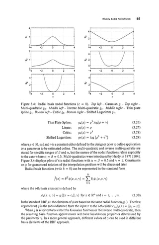
![86 APPROXIMATIONSTRUCTURES
3.4.2 Properties
Given a constant value for 7 ,three procedures are typical for the specification of the centers
Ci.
1. For a fixed batch of sample data {(zj,
Y~)}T=~,
when the objective is interpolation of
the data set, the centers are equated to the locations of the sample data: ci = zi for
i = 1,... N. Data interpolation for j = 1,. ..,N provides a set of N constraints
leaving ,& degrees of freedom. These interpolation constraints can be written as
Y = [@,',PT][ ;]
where @ and Y are defined in eqn. (2.Q P = [I)(z1), ..., p ( s ~ ) ] ,
p(z3) =
. . , p ~ ( z ~ ) ] ~ ,
and b = [bl,...,billT. Sinceg is a radial function, q5,(z3)=
g((1z3
-z,II) = $3 (
z
,
)
;
therefore, the matrix is symmetric. The RBF approximator
of eqn. (3.22) still allows an additional ,& degrees of freedom. The additional con-
straint that x
:
l 0,p3(z,) = 0 for j = 1,. . . ,& is typically imposed. The resulting
linear set of equations that must be solved for 0 and b is
This is a fully determined set of N +k equations with the same number of unknowns.
It can be shown that when g is appropriately selected, this set of equations is well-
posed [79]. The choice of g is further discussed below.
2. The c, are specified on a lattice covering D. Such specification results in a LIP
approximation problem with memory requirements that grow exponentially with the
dimension of s, but very efficient computation (see Section 2.4.8.4).Theorem 2.4.5
shows that this type of RBF is a universal approximator.
3. The c, are estimated online as training data are accumulated. This results in a NLIP
approximation problem. Theorem 2.4.4shows that this type of RBF is a universal
approximator. Theresulting approximator may have fewerparameters than case 2,but
the approach must address the difficulties inherent in nonlinear parameter estimation.
In addition, the computation saving methods of Section 2.4.8.4will not be applicable.
Although our main interest will be in approximation problems, the use of RBFs for data
interpolation has an interesting history. The analysis of the interpolation has implications
for the choice of g in approximation problems.
As described in Section 2.2,the LIP RBF interpolation problem with c, = z, is solvable
if the regressor matrix @ with elements q$3 = g(/Iz, - z311) is nonsingular (assuming that
k = 0). Therefore, conditions on g such that @ is nonsingular are of interest. An obvious
necessary condition is that the points {z2,
i = 1...,N}be distinct. This will be assumed
throughout the following.](https://image.slidesharecdn.com/adaptive-approximation-based-controlcompress-230219164415-f6eb4a64/85/adaptive-approximation-based-control_compress-pdf-104-320.jpg)
![CEREBELLAR MOOELARTICULATION
CONTROLLER 87
EXAMPLE3.6
Let g(r)= rz with r defined as the Euclidean norm, then in two dimensions (n= 2),
$i ( r )= (z- ~ i ) ~
+( y - ~ i ) ~ .
For this nodal function, the approximator EL,
Bi#i (r)
does not define an N dimensional linear space of functions. Instead, it defines a subset
of the linear space of functions spanned by (1,z, y, z2+y2). To see this, consider
that
N N
(3.32)
N
= Cel (z2 - 2z,z +.
p +Y2 - 2Y,Y+Y,z) (3.33)
,=1
= ~ ( 2
+Y2) +B~+cY+
D (3.34)
where the parameters in the bottom equation are defined by A = C,”=,
B,, B =
-2 E,=l
B,z,, C = -2 C,”=,
B,y,, and D = C,=l8%
(za +y,’). For general n,
the interpolation matrix will be singular if N > -1 + $ ( n+1
)
(
n +2
)
. Therefore,
g(r)= r2 with the Euclidean norm is not a suitable choice of radial basis function
when the objective is to interpolate an arbitrary data set using a RBF with centers
n
N N
defined by the data locations [219].
Let A be defined as the matrix with elements given by
A,, = 1
1
z
, - z
,
1
1
2
, z = 1,...,N , j = 1,.. . ,m. (3.35)
Note that A is symmetric with zero diagonal elements and positive off-diagonal elements
that satisfy the triangle inequality (i.e., A,, 5 A,l + Ai,) and = g(A,,). It can be
shown [167, 2191 that if the points ( 2 , ) are distinct in R”,
then the matrix A is positive
definite. Examples of singularity for other norms (e.g., the infinity norm) are presented in
[219].
The results of Micchelli [167] (reviewed in [79, 2191) give sufficient conditions on g ( . )
and k such that the RBF LIP interpolation problem is solvable. In particular, the Gaussian,
multi-quadratic, and inverse multi-quadratic RBF LIP interpolation problems are solvable
independent of n and N . For the linear nodal function the only additional constraint is that
N > 1. For the cubic nodal function, Q, is nonsingular if n = 1, but can be singular if
n > 1.
The relation of RBFs to splines is investigated in [204, 2191.
3.5 CEREBELLAR MODEL ARTICULATION CONTROLLER
The original presentation of the Cerebellar Model Articulation Controller (CMAC) [1, 21
discussed various issues that have been discussed elsewhere in this text. In addition, the
original presentation focused on constant, locally supported basis elements. This resulted
in piecewise constant approximations. A main contribution of the CMAC approach is
the reduction of the amount of memory required to store the coefficient vector denoted
herein by 8. Subsequent articles [4, 142, 1951generalized the CMAC approach to generate
smooth mappings while retaining the reduced address space of the original CMAC. The](https://image.slidesharecdn.com/adaptive-approximation-based-controlcompress-230219164415-f6eb4a64/85/adaptive-approximation-based-control_compress-pdf-105-320.jpg)
![88 APPROXIMATION
STRUCTURES
following presentation of the CMAC ideas is distinct from that of the original articles to
both incorporate the new ideas of the subsequent articles and to conform to the style of this
text. The flow of the analysis and some of the examples still follow the presentation in [2].
Applications involvingthe CMAChave been presented, for example,in [170,171,269,2701.
3.5.1 Description
For linear in the parameter approximators, the approximation can be represented in the form
&,= QT4(.)
where Q E RN and $ : D H RN.When $ is a vector of local basis functions defined on a
lattice, then as shown in Section 2.4.8.4, it is possible to define a function I ( z ): D H 2F
where 2~= { 1,. . , ,N}and 2
; is a set of m elements of 2 ~ .
The set 1(z)are the indices
(or addresses) of the nonzero elements of $
(
z
)
.
Throughout the discussion of the CMAC,
the parameter m is a constant. This implies that at any z E 2,there is the same number
m of nonzero basis elements. The motivation of this assumption will become clear in the
following. Therefore, the approximation off at zcan be calculated exactly and efficiently
f(z)= Q k d k ( z ) . (3.36)
by
k E I ( x )
At this point, an example is usekl to ensure that the notation is clear.
EXAMPLE3.7
Let z E D C Rdwith d = 2. Define 2)= [-1.11 x [-1,1]. Define the lattice so
that there are r = 201 basis elements per input dimension with centers defined by
(z2,y3) = (w,
w)for i , j E [I,2011. Let the basis elements for each input
dimension be defined by
4%(.) = x(a:- 2%) and $3 (Y)= X(Y - Y3)
where
1
0 otherwise.
if - 0.01 5 z < 0.01
The approximator basis functions for the region 2
,are defined as
4rC(Z,Y) = x ( z - d X ( Y - Y3)
where k(i,j ) = i +20l(j - 1).Note that the function k(i,j ) maps each integer pair
(i,j)toauniqueintegerinZ~= [1,40401].Foranypoint (z.y) E [-I, 1)x[--I, I),
the indices of the m = rd = 4 nonzero elements of the vector (
I can be directly
computed by
i(z) = floor(100Lz+ 100) +1
j(y) = fIoor(100y + 100) +1
I(z:y) = { ~ ( i l j ) , k ( z + l l j ) . ~ ( ~ ~ j + l ) , k ( ~ + l , j + l ) } ,
where I(z,y) is a four element subset of 2 ~ . D](https://image.slidesharecdn.com/adaptive-approximation-based-controlcompress-230219164415-f6eb4a64/85/adaptive-approximation-based-control_compress-pdf-106-320.jpg)
![CEREBELLAR MODEL ARTICULATION
CONTROLLER 89
Since the elements of the vector 4(z) with indices not in Z(z) are all zero and the indices
Z(z) are simple to calculate, locally supported lattice approximators allow a significant
reduction in computation per function evaluation. However, implementation of the ap-
proximator still requires memory3 for the N parameters in 0. The objective of the CMAC
approach is to reduce the dimension ofthe parameter vector 0 from N to M where M << N
without losing the ability to accurately approximate continuous functions over D.
H EXAMPLE33
Assume that z E D C 8
‘ and that the lattice specifies T basis functions per input
dimension. In this case, N = T’. The exponential growth implies that computational
and memory reduction techniques become increasing important as the dimension of
the input space increases. n
The CMAC separates the address space of the parameter vector from the indices of the
regressor vector through the introduction of a (deterministic) embedding function E(i) :
ZN H 2~where A4 <
< N. This results in the approximator being calculated as
f ( z )= o E ( k ) $ k ( Z ) . (3.37)
k E I ( x )
Note that the integers E(k)for k E I ( z )are not guaranteed to be unique. The advantage
of this representation is that the required physical memory to store O E ( k ) requires only M
locations. In the discussion that follows E(Z(zi))
will be used to denote the set {E(j)ijE
Z(zi)}
where ziE 8
‘ is the i-th evaluation point.
The embedding function E can be implemented, for example, by a hashing function
[1601. The embedding function is a deterministic function that maps each integer in [l,
N]
onto an integer in [l,MI. Since M < N the mapping E is not one-to-one. In fact, since it
is typical for M <
< N the mapping E is many-to-one. Example embedding functions are
k = mod(j,M )and k = ceil ( M rand (j))
where j E [l,N].In the latter example, “rand”
is a uniform pseudorandom number generator with seed j and with range [0,1] C 8’.
3.5.2 Properties
Let z’ and z2 denote two evaluation points. Using the index sets Z(z’) and Z(z2) it is
straightforward to see that adjustment of the parameters affecting f
(
z
)
jZ1 as calculated by
eqn. (3.37) will also affect (or generalize to) f*(x)I22as calculated by eqn. (3.37) when
I(z’) nI(z2)# 0,where 0 denotes the empty set. When the approximator is computed
by eqn. (3.36) and I(%’)nI ( z 2 )= 0,the lattice structure of the approximator is said to
dichotomize z1 from x2,in the sense that changing the parameters to adjust f(z)l,i does
not affect f ( z ) I z ~ .
When the function to be approximated is assumed to be continuous,
it is desirable to have generalization between nearby points and to dichotomize widely
separated points. The term learning interference is used to define the possibly negative
effects of training at z1that affects the value of f(z)lxz.
Introduction ofthe CMAC embedding function in eqn. (3.37 results in increased learning
interference. Thisistruesinceevenif1(z1)n1(z2) = 0itmay be thecasethat E (Z(z’))n
’Due to the lattice definition, the basis function parameters (z,, yj) need not be explicitly stored. Therefore, the
memory required to store the parameters used to calculate 4 is much less than N . Throughout this discussion the
memory required for the parameters necessary to compute 6 will be neglected.](https://image.slidesharecdn.com/adaptive-approximation-based-controlcompress-230219164415-f6eb4a64/85/adaptive-approximation-based-control_compress-pdf-107-320.jpg)
![CEREBELLAR MODEL ARTICULATION CONTROLLER 91
r M m
100 lO"0 m > d
100 1000 m > 2d
1000 100 m > I d
1000 1000 m > d.
B
All of these lower bounds on m are quite reasonable and easily satisfied. n
EXAMPLE 3.10
The purpose of this example is to illustrate that the choice of the embedding function
can have serious negative consequences for the capabilities of the approximator.
Assume that a function is to be approximated over the domain 23 = [0,1]x [0, 11.
Let (z,y) denote the two independent variables and define a lattice by
da: = 0.01, z
i= (i - 2)da, i = 1,...,103,
dy = 0.01, yj = ( j - 2)dx, j = 1,...,103,
so that N = 1032= 10609. Define the address of each node by
k ( i , j ) = (i- 1)103+j
which given the constraints on i and j has the inverse mapping
j = mod(k- 1,103)+1 (3.39)
k - j
103
a = - - - - $ 1 (3.40)
for k E [l,106091where mod(m,n) : I ++ [O, n - 1
1 is the modulus function that
returns the remainder of m divided by n. Given any ( 2 ,y) E 23,the nodal indices
(i.e., indices for the nearest lattice point) can be directly calculated without search as
i(x) = 2 +round(100x)
j(y) = 2 +round(100y)
(3.41)
(3.42)
which allows calculation of k(i,j ) as a function of position ( 2 ,y). Let the approxi-
mator use the basis functions for the nine nearest cells of 23,then
I(z,y)= { k ( i - 1 , j- l), k(i - 1,j), k(2 - 1 , j+l),
k ( i , j - I), k(i!j)l k ( i , j+I),
k(i +1 , j - l), k(2 +l,j), k(i +1,j+l)},
where i andj are computed from eqns. (3.41H3.42). Define the embedding function
to be
E(k) = mod(k - 1,M ) + 1, where M < N.
Although the conclusions of the example hold for almost any M < N , assume in the
following that M = 1000 so that the discussion can be explicit.
With the above design, (x,
y) E (0, ,005) x (0,.005) corresponding to i = 2,j =
2, k = 105 maps to the nodal and physical addresses
I(z,Y)
= E (I(., Y)) = (1, 2, 3,
104, 105, 106,
207, 208, 209).](https://image.slidesharecdn.com/adaptive-approximation-based-controlcompress-230219164415-f6eb4a64/85/adaptive-approximation-based-control_compress-pdf-109-320.jpg)
![MULTILAYERPERCEPTRON 93
Alternatively, when I ( z l )i
lI(z2)= 0,how can the designer determine the probability
that number of elements in E (I(z'))nE (I(z2))
is a particular value of n? Assuming
the the elements of E (I(zl))are unique and that the mapping E is uniform in the sense of
the previous paragraph, the probability that a single element of E ( I ( z 2 ) )
is in E ( I ( z l ) )
is q = s.The probability that the same single element of E (1(z2))is not in E (I(zl))
is p = 1 - q. The probability that n of the m elements of E ( I ( $ ) ) are in E (I(d))is,
by the binomial distribution,
m!
n!(m
- n)!
qnPm-n (3.43)
The results of evaluating this expression for various values of m, M , and n are displayed
in Table 3.2. The probability decreases rapidly with both n and M . Note that there are
tradeoffs involved in the selection of both m and M . Making m large decreases the average
contribution of each coefficient (data stored at the physical address) and increases the extent
of local generalization, but making m small decreases the amount of computation required
and decreases the probability of collisions between non-overlapping sets of nodal addresses
(i.e., interference). Selecting 111small decreases the physical memory requirements, but
increasing M decreases the probability of collisions between non-overlapping sets of nodal
addresses.
m =
M =
n=O
n=1
n=2
n=3
n=4
-
-
4 9 16 25
2000 2000 2000 2000
9.92e-1 9.60e-1 8.79e-1 7.30e-1
7.95e-3 3.91e-2 1.13e-1 2.31e-1
2.39e-5 7.06e-4 6.87e-3 3.51e-2
3.19e-8 7.45e-6 2.58e-4 3.41e-3
1.60e-11 5.05e-8 6.77e-6 2.37e-4
~
4 9 16 25
4000 4000 4000 4000
9.96e-1 9.80e-1 9.38e-1 8.55e-1
3.99e-3 1.99e-2 6.03e-2 1.34e-1
5.99e-6 1.79e-4 1.82e-3 1.O le-2
3.40e-9 9.44e-7 3.40e-5 4.90e-4
1.00e-12 3.19e-9 4.44e-7 1.69e-5
Table 3.2: Probability of n collisions for an physical memory of size M where each input
point maps to m addresses.
3.6 MULTILAYER PERCEPTRON
Perceptrons [223] and multilayer perceptron networks [226] have a long history and an
extensive literature [170, 2961. Examples of the use of multilayer perceptrons in control
applicationsarecontainedin [36,40,41,42,45,65, 101, 111, 116, 123, 148, 149, 172, 181,
209,211, 224,229, 244,2961.
3.6.1 Description
The left image in Figure 3.5 illustrates a perceptron [223]. The output of the perceptron
denoted by 2ri is
(3.44)](https://image.slidesharecdn.com/adaptive-approximation-based-controlcompress-230219164415-f6eb4a64/85/adaptive-approximation-based-control_compress-pdf-111-320.jpg)
![94 APPROXIMATION STRUCTURES
u,=bi+Ci,,,nxiw,i
.
/
.
p
h
J
Xn
Figure 3.5: Left-Single node perceptron. Right-Single layer perceptron network. The
bold lines in the right figure represents the dot product operation (weighting and summing)
performed by the connection and nodal processor.
Often for convenience of notation, this will be written as
vz = g (Wza)
where W, = [b,,w,lr..
. ,w,,]and z = [11zl,
. ..,a,].
The function g : 8
' H R1 is a
squashing function such as g(z) = atan(z)or g(a) = -. Note that the perceptron
has multiple inputs and a single output. If g(a) is the signum function, then a perceptron
divides its input space into two halves using the hyperplane u, = W,z. If u, < 0, then
vt = -1. If u, > 0, then v, = 1.If u,= 0, then v, = 0. This hyperplane is referred to as a
linear discriminant function.
The image on the right sideof Figure 3.5 shows anetwork that forms a linear combination
of perceptron outputs. The network output is
y = O
V
where VT = [vl, ... , v ~ ]
is the vector of outputs from each perceptron defined in eqn.
(3.44) and 8 E V x N
is a parameter matrix. This approximator is referred to as a single
hidden layer perceptron network. The parameters in W, are the hidden layer parameters.
The parameters in 0 are the output layer parameters. By Theorem 2.4.5, single hidden layer
perceptron networks are universal approximators. In the case that y is a scalar (i.e., q = l),
the function g(y) with g being a signum function defines a general discriminator function
that can be used for classification tasks [1521.
Ifdesired, networks with multiple hidden layers can be constructed. This is accomplished
by defining 8 to be a matrix so that y is a vector. If we define z = hg(y), then the network
has two hidden layers defined by the weights in W and 8.
The perceptron networks defined above arefeedforward networks. This means that the
information flow through the network is unidirectional (from left to right in Figure 3.5).
There is not feedback of information either from internal variables or from the network
output to the network input. In the case where some of the internal network variables or
outputs are fed back to serve as a portion of the input, we would have a recurrent perceptron
network. In this case, the network is a dynamics system with its own state vector. When
such recurrent networks are used, the designer must be concerned with the stability of this
network state.](https://image.slidesharecdn.com/adaptive-approximation-based-controlcompress-230219164415-f6eb4a64/85/adaptive-approximation-based-control_compress-pdf-112-320.jpg)
![MULTILAYER PERCEPTRON 95
Perceptron networks are sometimes referred to as supervised learning or backpropagation
networks, but neither ofthese namesare accurate. Supervised learning refer; to the approach
of training (i.e., adjusting the parameters) a function approximator y = f(z,6, u ) so that
the approximator matches, as closely as possible, a given set of training data described as
{(yi,zi)}El,In this scenario a batch of training samples is available for which the desired
output yi is known for each input 22.Many early applications of perceptron networks were
formulated within the supervised learning approach; however, any function approximator
can be trained using such a supervised learning scenario. Therefore, referring to aperceptron
network as a supervised learning network is not a clear description.
The backpropagation algorithm is described in Section 4.4.2.3.Although the algorithm
referred to as backpropagation was derived for perceptron networks, see e.g. [226], that
algorithm is based on the idea of gradient descent. Gradient descent parameter adaptation
can be derived for any feed forward network that uses a continuous nodal processor, see e.g.
[29I]. Therefore, referring to a perceptron network as a backpropagation network is again
not a clear description of the network. In addition, the fact that a multilayer perceptron
network can be trained using backpropagation is not a motivation for using these networks,
since gradient descent training is a general procedure that can be used for many families of
approximators.
3.6.2 Properties
The literature on neural networks contains several standard phrases that are often used to
motivate the use of perceptron networks. For any particular applications, the applicability
of these standard phrases should be carefully evaluated.
A typically stated motivation is that perceptron networks are universal approximators.
As discussed in Section 2.4.5, numerous families of approximators have this or related
properties. Therefore, the fact that perceptron networks are universal approximators is not,
by itself, a motivation for using them instead of any other approximator with this property.
A perceptron network with adjustable hidden layer parameters is nonlinearly parame-
terized. Therefore, another stated motivation is that perceptron networks have certain
beneficial “order of approximation” properties, as discussed in Section 2.4.1. On the other
hand, perceptron networks are not transparent, see Section 2.4.9. There are no engineer-
ing procedures available for defining a suitable network structure (i.e., number of hidden
layers, number of nodes per layer, etc.) even in situations where the function f to be
approximated is known. Also, since the network is nonlinearly parameterized, the initial
choice of parameters may not be in the basin of attraction of the optimal parameters.
Early in the history of neural networks, it was noticed that perceptron networks “offer
the inherent potential for parallel computation.” However, any approximation structure that
can be written in vector product form is suitable for parallel implementation on suitable
hardware. Interesting questions are whether any particular application is worth special
hardware, or more generally, is any particular approximation structure worth additional
research funding to develop special purpose implementation hardware, when hardware
optimized for performing matrix vector products already exists.
Another frequently stated motivation is the idea that perceptron networks are models
of the nervous systems of biological entities. Since these biological entities can learn to
perform complex control actions (balancing, walking, dancing, etc.), perceptron networks
should be similarly trainable. There are several directions from which such statements
should be considered. First, is a perceptron network a sufficiently accurate model of a
nervous system that such an analogy is justified? Second, is the implemented perceptron](https://image.slidesharecdn.com/adaptive-approximation-based-controlcompress-230219164415-f6eb4a64/85/adaptive-approximation-based-control_compress-pdf-113-320.jpg)
![96 APPROXIMATION
STRUCTURES
network comparable in size to a realistic nervous system? Even if those questions could
be answered affirmatively, do we understand and can we accurately replicate the feedback
and training process that occur in the biological exemplars? Also, the biological nervous
system may be optimized for the biochemical environment in which it operates. The optimal
implementation approach on an electronic processing unit could be significantly different.
Another frequent motivation for perceptron networks is by analogy to biological control
systems. It is stated that biological control systems are semi-fault tolerant because they
rely on large numbers of redundant and highly interconnected nonlinear nodal processors
and communication pathways. This is referred to as distributed information processing. To
motivate perceptron networks, it is argued that highly interconnected perceptron networks
have similar properties to biological control systems, since for perceptron networks the
approximator information is stored across a large number of “connection” parameters.
The idea being that if a few “connections” were damaged, then some information would be
retained via the undamaged parameters and these undamaged parameters could be adapted to
reattain the prior level of performance. However, the perceptron networks that are typically
implemented are much smaller and simpler than such biological systems, resulting in a
weak analogy. In addition, this line of reasoning neglects the fact that perceptron networks
are typically implemented with a standard CPU and RAM, where there is no “distributed
network implementation” since these standard items fail as a unit. Therefore, the CPU and
RAM implementation is not currently analogous to a biochemical network implementation.
3.7 FUZZY APPROXIMATION
This section presents the basic concepts necessary for the reader to be able to construct a
fuzzy logic controller. The presentation is self-contained, yet succinct. Readers interested
in a detailed presentation of the motivation and theory of fuzzy logic should consult, for
example, [21, 303,3041. Detailed discussion of the use of fuzzy logic in fixed and adaptive
controllers is presented, for example, in [15, 32, 63, 65, 67, 125, 131, 150, 151, 182, 184,
189, 198,230,261,266,267, 283,284,286, 3021. The main references for this section are
[67, 284, 3041.
3.7.1 Description
The four basic components of a fuzzy controller are shown in Figure 3.6. In this figure,
over-lined quantities represent fuzzy variables and sets while crisp (real valued) variables
and sets have no over-lining. This notation will be used throughout this section, unless
otherwise specified.
3.7.7.7 Fuzzy Sets and Fuzzy Logic Given a real valued vector variable x =
[zl,. ..,xnITthat is an element of a domain X = XIx X
z x . . I x X,, the region Xi is
referred to as the universe of discourse of xi and X as the universe of discourse of x.The
linguistic variable %i can assume the linguistic values defined by X i = X:,. ..,Xfi.}.
The degree to which the linguistic variable Z
i is described by the linguistic value X! is
defined by a membership function pL8;(z) : Xi H [0,1]. Common membership functions
include triangular and Gaussian functions. The fuzzy set 2;associated with linguistic vari-
able Zi,universe of discourse Xi, linguistic value X!,and membership function px: (z)
{](https://image.slidesharecdn.com/adaptive-approximation-based-controlcompress-230219164415-f6eb4a64/85/adaptive-approximation-based-control_compress-pdf-114-320.jpg)
![FUZZY APPROXIMATION 97
Fuzzification iGx Fuzzy ~ € 0
Inference ---
is
Defuzzification uEu
(3.45)
Note that fuzzy sets have members and degrees of membership. The degree of membership
is the main feature that distinguishes fuzzy logic from Boolean logic. The support of a
fuzzy set P on universe of discourse X is defined as Supp(P3)= {z E X I p p ( z )# 0). If
the Supp(F) is a single point z, and pp(z,) = 1,then z, is called afuzzy singleton.
EXAMPLE 3.11
To illustrate the concepts of the previous paragraph, consider a vehicle cruise control
application. Let the physical variables be z = [we, .IT, where u, = w -v,,w denotes
speed, w, denotes the commanded speed, and a denotes acceleration. The linguistic
variables are defined as 3 = [speederror,accele~ation]~.
The linguistic values for
Rule Base
Y
Figure 3.6: Components of a Fuzzy Logic Controller.
1.51 1
0.5
-15 -10 -5 0 5 10 15
Velocity error, mis
1.5
-2 -1.5 -1 -0.5 0 0.5 1 1.5 2
Acceleration, rnis
Figure 3.7: Membership functions for speed error and acceleration for the cruise control
example.](https://image.slidesharecdn.com/adaptive-approximation-based-controlcompress-230219164415-f6eb4a64/85/adaptive-approximation-based-control_compress-pdf-115-320.jpg)
![98 APPROXIMATION STRUCTURES
OR
maximum
algebraic sum
bounded sum
drastic sum
PAUB(”) = PA(X) CE P d Z ) AND PAnB(z) = PA(z) *PB (z) .
max(pA(z),p g ( z ) ) minimum min(pA(z), p g ( z ) )
PA(”) +p~g(z)
- p~(z)p,g(z) algebraic product p ~ ( z ) p ~ g ( z )
min(1, p ~ ( z )
+p g ( z ) )
‘ PA(.) ifpg(z) = O ’ p ~ ( z ) ifpg(z) = 1
{ p~g(z) if p ~ ( z )
= 0 drastic product < p g ( z ) ifpA(z) = 1
bounded product max(0, ~ A ( z )
+p~g(z)
- 1)
1 otherwise 0 otherwise
Table3.3: Example implementations of fuzzy logic (left) s-norm operations for A uB and
(right) t-norm operations for i?nB.
each linguistic variable could be defined as
X I = {Slow,Correct,~ a s t )
X2 = {Negative, Zero, Positive}
so that N1 = N2 = 3. Then, the space X is defined as
I
SN C N F N
X = X l x 8 2 = SZ C Z F Z
{ S P CP F P
where each linguistic value has been represented by its first letter. If the universe of
discourse is X = [-15,151 x [-2,2], then one possible definition ofthe membership
n
functions for XIand X 2 are shown in Figure 3.7.
In fuzzy logic, the “Aor B” operation is represented as ‘‘AuB.” The membership
function for the fuzzy set Au B is calculate by a s-norm operation [284] denoted by $,
p~,,g(z) = p ~ ( z )
@ pg(z). In fuzzy logic, the “Aand B” operation is represented
as “AnB.” The membership function for the fuzzy set A nB is calculate by a t-norm
operation [284] denoted by *,p ~ , , ~ ( z )
= p ~ ( z )
*p~g(z).
Table 3.3 contains several of
the possible implementations of the * and @ operations. The membership function for the
complement of fuzzy set i? is p ~ ~ ( z )
= 1- p ~ ( z ) .
The fuzzy complement is used to
implement the “not” operation
EXAMPLE 3.12
Figure 3.8 presents examples of the operations discussed in the previous paragraph
for the fuzzy system described in Example 3.11. The algebraic product is used to
implement the * operator. The left mesh plot shows the membership function for
the fuzzy set “velocity error is fast and acceleration is positive” (i.e., p ~ ~ p ( v ,
a) =
pp(v)pp(a)). The center plot shows the membership function for the fuzzy set
“acceleration isnegative and acceleration is zero” (i.e.,p~,,,q
(a,a) = pz (a)pn(a)).
The right plot shows the membership function for the fuzzy set “acceleration is not
n
negative” (i.e., p ~ ~ ( a )
= 1- pN(a)).
Afuzzy relation Q(U,
V) between the the universe of discourses U and V is a fuzzy set
defined on U x V:](https://image.slidesharecdn.com/adaptive-approximation-based-controlcompress-230219164415-f6eb4a64/85/adaptive-approximation-based-control_compress-pdf-116-320.jpg)
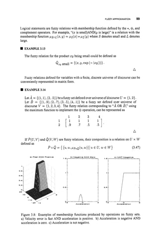
![100 APPROXIMATION STRUCTURES
where
PLp0Q(Ww)= max [t(PLp('LL,v),PQ(? w))] (3.48)
and t represents a t-norm (see Table 3.3). Computation of the membership functions for
compositions of fuzzy relations can be difficult when the universes of discourse involve
continuous variable. When the universes of discourse involve a finite number of discrete
variables, computation can be efficiently organized through algebra similar to matrix mul-
tiplication.
VEV
w EXAMPLE 3.15
Let P(2,y) be the fuzzy relation 2 < y for 2,y E
function
described by the membership
1
PP(Z?Y)= -.
P Q ( Y > Z )= -
.
Let Q(y, z ) be the fuzzy relation y < z for y, t E 8
'described by the membership
function
1
Then the membership function for the composition P oQ,using the algebraic product
for the t-norm, is
r 1
(3.49)
Derivation of eqn. (3.49) is requested in Exercise 3.9. Examples such as this, where
n
~ L ~ , , Q ( x ,
z ) can be explicitly solved, are the exception.
EXAMPLE 3.16
Let the relation R(U,V )be represented by the matrix [304]
[ ::::::
]
[ :::;:;
]
and let the relation g(V,W )be represented by the matrix
If the t-norm is implemented by the min operation, then the composition R o ,
!
? is
represented as
R o
= [ 0.3 0.8 ] [ 0.5 0.9 ]
0.6 0.9 0.4 1.0
1
max(min(0.3,0.5),min(0.8,0.4)) max(min(0.3,0.9),min(0.8,l.O))
max(min(0.6,0.5), min(0.9,0.4)) max(min(0.6,0.9),min(0.9,l.O))](https://image.slidesharecdn.com/adaptive-approximation-based-controlcompress-230219164415-f6eb4a64/85/adaptive-approximation-based-control_compress-pdf-118-320.jpg)
![FUZZY APPROXIMATION 101
n
With these basic tools of fuzzy systems available to us, we are now ready to consider the
components of the fuzzy controller shown in Figure 3.6.
3.7.7.2 Fuzzification The previous subsection has introduce various aspects of fuzzy
logic as operations on fuzzy sets. Since control systems do not directly involve fuzzy sets,
a fuzzification interface is used to convert the crisp plant state or output measurements into
fuzzy sets, so that fuzzy reasoning can be applied.
Given a measurement z* of variable z in universe of discourse X,the corresponding
fuzzy set is X = {(z, p(z : z*)}. A few common choices are singleton, triangular, and
Gaussian fuzzification. For singleton fuzzification,
1 i f z = z *
0 otherwise.
p(x : z*) =
For triangular fuzzification,
p(z : z*) = { 1 - 9 i f l z - z * l < x
0 otherwise.
For Gaussian fuzzification,
In each of the above cases, the parameter X can either be selected by the designer or adapted
online.
Thefuzzijcation process converts each input variable z* into a fuzzy set X.Singleton
fuzzification is often used as it greatly simplifies subsequent computations. Other forms
of fuzzification may be more appropriate for representing uncertainty (or fuzziness) of the
control system inputs due, for example, to measurement noise.
3.7.1.3 Fuzzy implication Thefuzzy rule base will contain a set of rules {R',1 E
[l,...,N ] }ofthefom
R': IF (21 is XI1) and .. . and (2.. is Xk) THEN (iiis @') (3.50)
where li E (1,.. , ,Nil and 8 is the set of linguistic values defined for the fuzzy control
signal a. Each term in parenthesis is an atomicfuzzy proposition. The antecedent is the
compound fuzzy proposition:
z11s X p ) and ... and (
3
.
. is X ? ) .
A' = (- (3.51)
Each antecedent defines a fuzzy set in X = X I x . .. x Xn.The antecedent may con-
tain multiple atomic fuzzy propositions using the same variable and need not include all
fuzzy variables. The membership function for ALis completely specified once the t-norm](https://image.slidesharecdn.com/adaptive-approximation-based-controlcompress-230219164415-f6eb4a64/85/adaptive-approximation-based-control_compress-pdf-119-320.jpg)
![104 APPROXIMATION
STRUCTURES
similar to the idea of coverage discussed in Section 2.4.8.1. Two methods of inferring the
output of a rule base are possible: compositional inference and individual rule inference.
In compositional inference (see Section 7.2.1 in [284]), the relations corresponding to
each rule are combined (through appropriately selected logical operations) into one relation
representing the entire rule base. Then, composition with the input fuzzy sets is used to
define the output fuzzy set. The composition of all the rules into a single relation can
become cumbersome.
In individual rule inference, the output fuzzy set U
i = {(u:
pjp (u))}
corresponding to
each individual rule is determined according to eqn. (3.54). The output of the inference
engine, based on the entire (1 rule) rule base, then has membership function described by
either
(3.55)
(3.56)
Eqn. (3.55) is used when the individual rules are interpreted as independent conditional
statements intended to cover all possible operational situations. Eqn. (3.56) is used when
the rule base is interpreted as a strongly coupled set of conditional statements that all should
apply to the given situation. For example, given Mamdani product implication, eqn. (3.55),
with the “or” operation implemented as max, the output membership function is
P R B ( u ) = max sup ( P x ( z: z*)p.xl(z)PB.(u))].
“ [Z€X
(3.57)
Note that the resulting rule base membership function may be multimodal or have discon-
nected support.
3.7.1.5 Defuzzification The purpose of the defuzzifier is to map a fuzzy set, such as
0= (u,
~ R B
(u))
for u E U, to a crisppoint u*in U.
The point u*should be in some sense
“most representative” of U . Since there are many interpretations of “most representative,”
there are also many means to implement the defuzzification process.
Table 3.5 summarizes three methods for performing defuzzification. The first method
computes an indexed center ofgravity. This method is often computationally difficult since
the rule base membership function is typically not simple to describe. The middle row of
the table describes the center average defuzzification process. The function “center” could,
for example, select the midpoint of the set { u E U l p h (u)
> 0 1. The center average is
computationally easier than the indexed center of gravity approach. The final row of the
table describes the maximum defuzzification process. The set hgtRB(U) contains all values
ofuthat achieve the maximum value OfpRB (u)
over U.The functiong processes hgtRB(U)
to produce a unique value for u*. The function g could for example select the minimum,
center, or maximum of hgt,, (U).
3.7.2 Takagi-Sugeno Fuzzy Systems
This subsection presents the Takagi-Sugeno fuzzy system. The reasons for presenting this
special case are (1) it is commonly used, (2)it is rather straightforward to understand, (3) its
parametric form is amenable to stability analysis, and (4) it highlights the parallels between
fuzzy approximators and the other approximators discussed in this chapter.
The Takagi-Sugeno fuzzy system uses rules of the form
R1:IF (21 is and ... and (5nis Xk) THEN (fi = fi(z)). (3.58)](https://image.slidesharecdn.com/adaptive-approximation-based-controlcompress-230219164415-f6eb4a64/85/adaptive-approximation-based-control_compress-pdf-122-320.jpg)
![FUZZY APPROXIMATION 105
Indexed Center of Gravity
J, I I R B ( U ) U . ~ U
=
u, = {uE ~ I P R B ( U )
2 a )
c, = center ({uE U I p ~ " ( u )
> 0))
Table 3.5: Example methods of defuzzification.
For the fuzzy logic controllers that are of interest in this book, fi(z)is a parameterized
function (e.g., fi (z : e l ) )where the parameters are identified based on experimental data.
Typically,
n
but nonlinear functions in either z or 8 can be used. The membership function for the
antecedent is formed as in eqn. (3.52). The Takagi-Sugeno approach then calculates the
output control action as
Note that this approximator has the form of a basis-influence function with basis set {f,(z:
0,)) and influence functions {
r
,
(
z
)
}
.If the fuzzy rule set is complete and each PA, (z) is
finite, then this set of influence functions {r,(z))
will be finite, vanish nowhere, and form
a partition of unity.
Eqn. (3.59) has a variety of interesting interpretations. The f,(z)
can be previously
existing operating point controllers or local controllers defined by human "experts." Alter-
natively, this expression can be interpreted as a "gain scheduled" controller. In all these
cases, it is of interest to analyze the stability of the nonlinear closed-loop control loop that
results.
3.7.3 Properties
One of the early motivations for fuzzy systems was there transparency, in the sense that
users can (linguistically) read, describe, and understand the rule base. Similarly, a fuzzy
system such as the Takagi-Sugeno type is similar to a smoothly interpolated gain scheduled
controller, where each control law fiis applicable over the support of ri.
Fuzzy systems are capable of universal approximation, see for example Chapter 9 in
[284]. Adaptation of fuzzy systems, as with any approximator, must be approached with
caution. If for example the antecedents of the rule base are adapted, this is a nonlinear
estimation process. Adaptation of the antecedents could lead to loss of completeness of the
fuzzy rule base.](https://image.slidesharecdn.com/adaptive-approximation-based-controlcompress-230219164415-f6eb4a64/85/adaptive-approximation-based-control_compress-pdf-123-320.jpg)
![106 APPROXIMATION
STRUCTURES
3.8 WAVELETS
Efficient allocation of approximator resources motivates the tuning of approximator basis
functions to the local curvature properties of the function. Similar motivations arise in
various application fields. For example, in signal (and image) processing it has proven
useful to decompose signals (and images) using a space of basis functions that have local
support both in the time and frequency domains. Such motivations across various fields
has lead to the development of wavelets, which means small waves. The main references
for this section are [51,60, 260, 262, 3061. A very understandable review of wavelets
is maintained on the website of R. Polikar [206]. Example articles discussing the use of
wavelets in control applications include [22, 37, 217, 2621.
Wavelet algorithms are defined to process data at different scales of resolution in both the
time and frequency domains. For our function approximation purposes, we are dealing with
a variable zinstead of time. Therefore, we will refer to the space and spatialfrequency
domains. For a function f(z) in the spatial domain, we will use the notation Ff([)
to
denote the Fourier transform o f f where E is the spatial frequency variable. The spatial
wavelength is D = 1,
t
The continuous wavelet transform is defined as
(3.60)
where 1c, is a real valued mother wavelet, 'T is the translation parameter, and D is the scale
parameter. Eqn. (3.60) is an inner product between the function f and the scaled and
translated mother wavelet. For fixed values of 'T and u, the wavelet transform Q?('T,a)
quantifies the similarity between f and the wavelet at that scale and translation. The
variable 'T shifts the mother wavelet along the x-axis. The mother wavelet $
J is selected
to have localized support which allows characteristics off to be accurately resolved along
the x-axis when a is small. The variable a allows analysis o f f at different scales. As 0
is increased, the inner product considers a wider range of 3: which includes lower spatial
frequencies. Similarly, as D is decreased the inner product considers a narrower range of z
and higher spatial frequencies.
The continuous wavelet transform is invertible by
if the admissibility constant cQ satisfies
(3.61)
where 4 = F$ is the Fourier transform of $(z). For the condition of eqn. (3.61) to be
true, it is necessary that d(0)= 0 which is equivalent to
]f(z)dz= 0. (3.62)
Examples of two real-valued wavelets are the Mexican hat (or Maar function) described
as
w,h(z) = A (1- z
'
) e-*"*,](https://image.slidesharecdn.com/adaptive-approximation-based-controlcompress-230219164415-f6eb4a64/85/adaptive-approximation-based-control_compress-pdf-124-320.jpg)
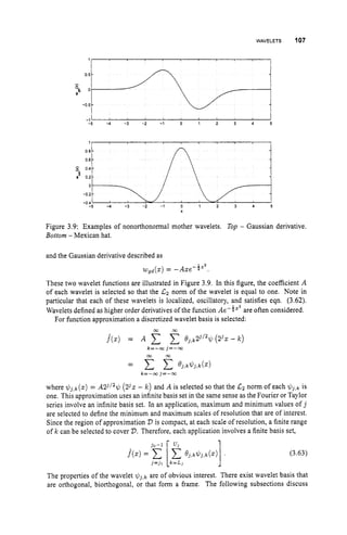
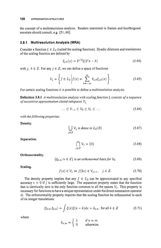
![WAVELETS 109
When this orthonormality condition is satisfied, then for a function g E Lz if we wish to
minimize Ilf - 9
1
1 for f E V,, the optimal value for the parameter 03,k in eqn. (3.65) is
defined uniquely by the Fourier coefficient:
O,,k = / g ( z ) t ~ , k ( z ) d z .
The main advantage of orthonormality is that the computation of the k-th coefficient of the
expansion of a function 9 in V, is independent of the the i-th coefficient or basis function
of that space. This greatly simplifies computations.
EXAMPLE 3.19
The simplest scaling function to satisfy these conditions is the characteristic function
on the unit interval
With this scaling function, Vo is the set of functions that are piecewise constant
between integers. The space V j is the set of functions that are piecewise constant
on each interval [$,5).
Since the functions that are piecewise constant on the
half integer intervals includes the set of functions that are piecewise constant on the
integer intervals, it is clear that VOC V1. Repetition of this reasoning can verify the
nesting condition of eqn. (3.66). Direct integration of
- W -c€
t H ( z ) c H ( z -j) = 1,X [ O . l ) ( ~ ) X [ O , l ) ( ~
- j) = X [ o , l ) ( ~ ) X [ j , J + l ) ( ” )
= 0
1,
shows that the orthonormality condition is satisfied. n
The MRA definition shows that { & , n } n E ~
is an orthonormal basis for Vj. The fact that
the Vj are dense in Lz means that {[j,n}j,ncz
is a basis for L2; however, the elements of
{ t j , n } n E ~
are not necessarily orthonormal to the elements of { [ k , n } n E Z for k # j . There-
fore, the dilations and translations of the scaling function do not provide an orthonormal
basis for Lz.
If we define W, to be the orthogonal complement of V, in Vj+l,then
Vj+l = vj a
3 Wj. (3.72)
In particular, we will call the function $J the wavelet generated by the scaling function [,
if its translates are mutually orthonormal (i.e., s$(z - k)$(z - m)dz = bk,m for all
k ,m E Z),are orthogonal to (i.e., s$
(
z - k)<(z - n)dz = 0 for all k ,TI E Z),and
form basis for WO.
The wavelets of resolution j are then defined as
$ j , k ( W ) = 2 i / 2 $ J ( 2 i ~
- k ) , j,k E z. (3.73)
The set { $ , , k } k E Z is an orthonormal basis for W j .Fortunately, whenever a M U exists,
there exist a wavelet that can be constructed from the scaling function. This construction
process is not straightforward. For details on the construction of the wavelets, the reader is
referred to [60].](https://image.slidesharecdn.com/adaptive-approximation-based-controlcompress-230219164415-f6eb4a64/85/adaptive-approximation-based-control_compress-pdf-127-320.jpg)
![WAVELETS 111
rectangular box of a given width, and the coefficients of the expansion are the averages
the function taken over the support of the boxes. In the wavelet approach, the scaling
function and its translates will be used in conjunction with the wavelets that it gen-
erates. The scaling function for the Haar basis captures the average (low frequency)
behavior, while the wavelets capture the variation (higher frequency) behavior of the
function. An advantage of the wavelet approach is that due to the orthogonality and
local support ofthe basis functions, new basis elements can be added locally as needed
n
without affecting the values of the preexisting basis functions.
The Haar basis wavelet function isused throughout this section as it is straightforward to
understand and is useful for illustration of wavelet concepts. Applications where there are
constraints, such as smoothness of the approximation, motivate the use of other orthogonal
wavelets with compact support. Alternative wavelets have been formulated in literature.
For example, a class of orthogonal wavelets called Daubechies wavelets also are compactly
supported. Further, there are classes of orthogonal wavelets such as Meyer wavelets, and
Battle-Lemarie wavelets that vanish rapidly outside a compact support. For a detailed study
of orthogonal wavelets, the reader is referred to [60].
Let us consider the problem off approximating the function f over the compact set V.
Let 11,be a compactly supported orthogonal wavelet and E, the associated scaling function
as defined in Section 3.8.1. Let Vj be an MRA and Wj be as defined in eqn. (3.72). If
((w)
is the scaling function that generates the space V,with &,k(w)
defined as in (3.64),
then from properties (3.66) and (3.67) of the MRA, we get that given any c > 0, there exist
an integer j o , and a function f(w; p) given by
W
k = - w
such that
with pT = (.. ,p-1, PO,p l , ' .). Since V is a compact set, if the scaling function has a
compact support, we can write
llf(w) - h P ) I l < E
for some L, U E 2.
From (3.66)-(3.69) and (3.72) we have
Hence we can write the approximation for f uniquely as
The summation inside the square brackets is carried out over orthogonal wavelet translates
of a particular resolution. The left summation is carried out over resolutions higher than j1.](https://image.slidesharecdn.com/adaptive-approximation-based-controlcompress-230219164415-f6eb4a64/85/adaptive-approximation-based-control_compress-pdf-129-320.jpg)
![112 APPROXIMATION STRUCTURES
The summation involving E j , ,k is carried over orthogonal translates of the scaling function,
at the lower resolution level, j,. Thus (3.78) can be seen as reflecting the fact that any
function in L2 can be decomposed into a scaling function of resolution j, and wavelets
of higher resolution, with the highest resolution depending upon the desired accuracy of
approximation. The analysis leading to (3.78) can be carried out for any wavelet with com-
pact support, with the unique decomposition being a direct sum rather than an orthogonal
sum. However, an explicit use of orthogonality is needed for the next step.
The accuracy of approximation can be improved by increasing j o . Due to the orthog-
onality of the scaling and wavelet functions, the new approximation is obtained from the
existing approximation, simply by adding more basis functions, and evaluating the coef-
ficients corresponding to the new basis elements. The coefficients of the existing basis
hnctions remain the same. New basis elements need to be added only where the function
varies rapidly. Care must also be taken, since, as the resolution increases it may be difficult
to obtain enough samples to accurately estimate the parameters corresponding to the high
resolution wavelets.
3.9 FURTHER READING
This chapter has briefly introduced various approximation structures. Several of these
structures have entire books or journals devoted to their study. Therefore, we have only
touched the surface in this chapter. Sample references, in addition to those included directly
in the text, to publications providing additional information about specific approximator
structures are: polynomials and splines [52, 53, 55, 56, 57, 59, 62, 71, 238, 2401, CMAC
[l, 2,4, 125, 142, 170, 187, 1951,fuzzylogic [15,21, 63,67, 131, 150, 182, 184, 198,201,
285, 283, 284, 302, 303, 3041, radial basis functions [30, 31, 35, 79, 193, 204, 205, 219,
232,2901, neural networks [88, 108, 109, 110, 117, 152, 172, 186, 188, 190,203,211,223,
226,280,287,2981, and wavelets [22, 37, 51,60,260, 281, 3061.
3.10 EXERCISES AND DESIGN PROBLEMS
Exercise 3.1 The purpose of this exercise is to exhibit the effect that spatially localized
training samples can have on an approximator composed of basis elements with global
support.
Consider the approximation of the function f(z)= sin(7rz) over the interval V =
[-l: 1
1by a third order polynomial. The approximator is f(z)= x:=o
0,4t(z) where the
basis functions are the first four Legendre polynomials defined in eqn. (3.10). Theparameter
vector 8
,= [Qo,. . .,031 = [O.OOOO; 0.9549,0.0000,-1.15821 is the least squares optimal
set of parameters over V after truncation to four decimal places. This parameter vector
results in the Lz approximation error
-1
[/:
- ( j ( z )- f ( ~ ) ) ~ d z ]
= 0.0937.
The L, approximation error over 7
7 is about 0.2.
1. NumericallycomputedtheCz approximationerror over [-1.0,1.0] andover [0.5,1.0].
2. In control applications, the system may operate in the vicinity of any given operating
point for an extended period of time. This results in training samples arriving from a](https://image.slidesharecdn.com/adaptive-approximation-based-controlcompress-230219164415-f6eb4a64/85/adaptive-approximation-based-control_compress-pdf-130-320.jpg)
![EXERCISESAND DESIGN PROBLEMS 113
small subset of the domain Dfor that period oftime. In this exercise, we will simulate
this by selecting training samples only from the region D1 = [0.5,1.0). Randomly
generate 1000 training points z
iin D1.At each xi,compute the (noise free) value
of f(zi)= sin(.irzi). Update the approximation parameter vector using recursive
least squares as defined by eqns. (2.23) and (2.24). Initialize the parameter vector
as O0 and f‘k = A;’ = I . Use uniform weights Wk = 1. Save the sequence 6’i for
i = 100,200,... ,1000.
3. Using 8, for i = 100,200,.. . ,1000, compute the L2 approximation error over
[-1.O,l.O] and over [0.5,1.0].Plot these values versus the training iteration i.
You should see the Cz error over [-1.0,1.0] increasing (not monotonically) and the Lz
error over [0.5,1.0]decreasing. Why? How would an approximator with locally supported
basis elements perform differently?
Exercise 3.2 Select a low order polynomial function such as f(z)= 1 + z. Although
this is a polynomial function, assume that its functional form is not known and that this
unknown function is to be approximated based on noise corrupted measured data. Let m
be an integer value varying from the order of f(z)
to approximately 10. For each value of
m:
for i = 0, .. .,m by
evaluating f(zi)
and adding a small amount of random noise (e.g., Gaussian random
noise with standard deviation o = 0.1). Denote the vector of these measurements by
2. Fit an m-th order polynomial to the measured data {
(
q
,
$i)}zo.
Note that this is
an interpolation problem. Use the natural polynomial basis &
(
z
) = [l,
z,
. ..,P].
Let Om denote the resulting set of parameters such that Gi= Cp,(zi)O,.
3. Generateanew setofevaluationpoints(e.g., z= [0,0.01,.. . ,0.99! 11. Evaluateboth
the original polynomial f(z)= 1+zand the approximated polynomial p m ( z ) =
q
5
,
(
z
)
O
, at each of these evaluation points. Plot zversus both f and p,. What
happens as the order of the interpolating polynomial m increases?
Exercise 3.3 Repeat Exercise 3.2, but use alternative choices of basis functions. Include
at least one choice of basis functions that are defined to form a partition of unity.
Exercise 3.4 Select a low order polynomial function such as f(z)= 1 +z.For each
n = 11,.. .,100:
1. Generate m +1noise corrupted “measurements” at z, = i *
5.
1. Generate a set of evaluation points defined as zi= i *
2. Generate a set of noise corrupted “measurement” data jji = f(q)
+v, where v, is
3. Find Olo(n)to result in a least squares fit of a tenth order polynomial p l o ( z ) =
@lo(z2)6’lo(n)
to the measurement data {(xi,
&)}:=,, where &o(z) is a basis for the
space of 10-th order polynomials defined on [0,1].Note that this is an approximation,
not an interpolation, problem.
for i = 0,.. . ,n.
Gaussian random noise with standard deviation B = 0.1.
4. Evaluate the approximation accuracy defined by the Lz norm of the approximation
error
(f(z)- $l0(z~)Q10(n))~dz.](https://image.slidesharecdn.com/adaptive-approximation-based-controlcompress-230219164415-f6eb4a64/85/adaptive-approximation-based-control_compress-pdf-131-320.jpg)
![114 APPROXIMATION
STRUCTURES
5. Evaluate the sample variance of the approximation error
as a function of n.
Plot e(n) and v(n)versus n.
Exercise 3.5 Repeat Exercise 3.4, but use alternative choices of basis functions. Use at
least one choice of basis functions that are defined to form a partition of unity. Keep the
dimension of the basis vector fixed at 11.
Exercise 3.6 Write a program to interpolate the function
at the points z
i = -5+ 10 (A)for i = 0, ...,m, using an m-th order polynomial. For each
value of m, denote the interpolating polynomial by p,(z). Use odd values of m E [3;211.
For each value of m and for z E [-5,5]: (1) plot f and pm(z)versus z; and, (2) plot the
error E ( z )= f(z)-pm(z)versus z. Be certain that each plot includes several evaluation
points between each pair of interpolation points. Numerically compute
r5
Plot e(m) versus m. (See Section 3.6 in [240] for a discussion of issues related to this
exercise.)
Exercise 3.7 Repeat Exercise 3.6, but use an alternative choice of basis functions (e.g.,
splines or radial basis functions) that are defined to form a partition of unity.
Exercise 3.8 Consider the problem of estimating the vector 0 to minimize the two-norm
of the error between Y and aT0subject to the constraint that GB = 6, where Y E RM is
known, E R N x Mis known, B E gNis unknown, G E R J x is known, and 6 E RJ is
known. This is the restricted least squares problem [82, 1641. Use the method of Lagrange
multipliers to show that the the optimal constrained parameter estimate is
Exercise 3.9 In Example 3.15 ,confirm eqn. (3.49).](https://image.slidesharecdn.com/adaptive-approximation-based-controlcompress-230219164415-f6eb4a64/85/adaptive-approximation-based-control_compress-pdf-132-320.jpg)
![FORMULATION FOR ADAPTIVE APPROXIMATION 119
EXAMPLE4.1
Consider the linear model
y = ay +bu
where u(t)is the input, y(t) is the output and a, b are unknown parameters to be
estimated online. In the parameter estimation and adaptive control literature there
are various parametric models that have been proposed. We consider the following
parametric model and online learning scheme:
1
S + X
1
S + X
y = - [ ( a + X ) y + b ~ ]
y = -[(u+X)y+bu],
where X > 0 is a design constant. In the above formulation, we use the notation
y = H(s)(z],
where y ( t ) is the output of a linear system represented by the transfer
function H ( s )with z(t)as input (see Figure 4.3). Although this notation mixes the
time signals z(t),y ( t ) with the Laplace based transfer function H ( s ) ,it turns out to
be quite convenient in describing filtering schemes and therefore is used extensively
in the adaptive control literature of continuous-time systems [I 19, 179, 2351 and in
the remainder of this book. If the initial conditions of the filter are non-zero then
there will be an additional term for the initial conditions, however, for simplicity here
we assume that the initial conditions are set to zero.
Figure 4.3: Block diagram ofthe notation y = H(s)[z].
Let e = y - y be the output estimation error. The update laws for u,b are
generated as follows, based on the so-called Lyapunov synthesis method, which will
be described later in the chapter:
& = -71 ey
b = -72eu
where 71, 7 2 are positive design constants representing the adaptive gain for the
update algorithm of &(t)
and b(t)
A simulation example usingthe above identification schemeis shown in Figure 4.4.
We consider two input scenarios. In the first case, u(t)= sin(2xt)and in the second
case u(t)= 3 exp(-t/100). For simulation purposes, the unknown parameters are
assumed to be a = -1, b = 1, while the design constants are set to: X = 2,
y1 = 7 2 = 10. The top two plots of Figure 4.4 show the results for u(t)= sin(2rt),
while the bottom two are for the second case of u(t)= 3 exp(-t/100). As seen from
the plots, in both cases the output estimation error converges to zero. In fact, in the
second case the output estimation error converges to zero faster, as compared to the
first case. However, the parameter estimates converge to their true values (-1 and
1,respectively), only in the first case, where u(t)= sin(2n-t). This is related to the](https://image.slidesharecdn.com/adaptive-approximation-based-controlcompress-230219164415-f6eb4a64/85/adaptive-approximation-based-control_compress-pdf-137-320.jpg)
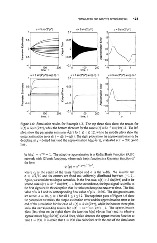
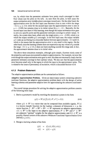
![DERIVATIONOF PARAMETRIC MODELS 129
4.2.2 FilteringTechniques
Frequently in applications only IC is available for measurement. The use of differentiation to
obtain x is not desirable. Therefore, the assumption of k being available should be avoided.
One way to avoid the use of differentiators is to use filtering techniques. By filtering each
side of (4.8) with a stable first-order filter A,where X > 0, we obtain
(4.11)
where z(t) = (z(t),u(t))
is the input vector to the adaptive approximator f,~ ( t )
is a
measurable variable computed as
(4.12)
AS x
X(t)= s+x["(t)l - s+x[fo(4t),'1L(t))l
and 6(t)is the filtered MFAE:
(4.13)
It is noted that in deriving (4.12) we use the fact that k(t)= s[z(t)].
form (4.4) described in Section 4.1.3, where the filter W(s)is given by
The reader is reminded that the parametric model described by (4.11) is of the general
and Inxnis the n x n identity matrix. Therefore, in this case, the matrix transfer function
consists of n identical first-order filters. The parameter X > 0 is a design parameter that
could influence the convergence rate of the adaptive scheme.
A reader may ask: what's the use of rewriting (4.5) as (4.1I), since the functional
uncertainty in f* is still present in the form of 6? The answer to this question is that
the magnitude of the uncertainty f
' can be significantly larger than the magnitude of the
filtered MFAE 6. Moreover, the magnitude of 6 can be further reduced, if desired, by
increasing the dimension ofthe basis vector $(z)in the adaptive approximator. In the limit,
as this dimension increases toward infinity,the MFAE ef converges to zero (over a compact
domain), as shown by universal approximation results. Since 6 is small, it can be more
easily accommodated in the nonlinear identification and control design. The "price" paid
for reducing the uncertainty from f*to 6is the presence of unknown parameters .Q* and c*,
which need to be estimated online. This cost becomes a design tradeoff, in the sense that
the smaller the dimension of @(z)(or the number of adjustable parameters) that are used
the smaller the difference between f
' and 6.
EXAMPLE4.4
Consider the second-order system
x1 = 2 2 -91(22)
x, = 2
1 +9
2
(
2
1t 22) +2u
where g1 and g2 are the unknown functions. In this example, fo and f* are given by](https://image.slidesharecdn.com/adaptive-approximation-based-controlcompress-230219164415-f6eb4a64/85/adaptive-approximation-based-control_compress-pdf-147-320.jpg)
![DERIVATIONOF PARAMETRICMODELS 131
4.2.3 SPR Filtering
Instead of the simple filter A,the designer can select to use a more complicated filter
W(s).In this case, by filtering each side of(4.8)with an appropriate stable filter W(s),
we
obtain
X ( t ) = W ( s )[f^(z(t);@*,u*)]
+W), (4.14)
where b(t)and X ( t ) are given by
6(t) = W S ) [ef(4t)l4t))l (4.15)
X ( 4 = sW(s)[Wl- W S ) [fo(m
4t))l' (4.16)
For reasons that will become apparent in the subsequent analysis of the adaptive approx-
imation scheme using the general filter W(s),
we assume that W(s)is a strictly positive
real (SPR) filter. A detailed presentation of SPR function and their properties is beyond the
scope of this book. A thorough treatment of the SPR condition and it's use in parameter
estimation problems is given for example in [119,2351. Some of the key features of SPR
functions that will be used subsequently are summarized in Section A.2.3of Appendix A.
4.2.4 Linearly ParameterizedApproximators
The nonlinear system (
4
.
5
)
-
(
4
.
6
)can be rewritten as a parametric model of the form (
4
.
11)
whether the adaptive approximator used is linearly or nonlinearly parameterized. However,
in the special case of a linearly parameterized approximator, a different type of parametric
model can be derived.
It is recalled that for linearly parameterized approximators, u is selected a priori, and
therefore the approximation function f can be written as f(z;O*, a*)= @*T4(z).There-
fore, the parametric model (4.11) becomes
(4.17)
Since 0' is a constant vector, it can be pulled in front of the linear filter, resulting in
X ( t ) = e*Tc(t)+b(t): (4.18)
where ( ( t )is a vector offiltered basis functions; i.e.,
Of course, the extension also works when (4.14)
is used with the more general filter W(s).
It is interesting to note that the parametric model (4.18)
is an algebraic equation with
the unknown coefficient vector 8' appearing linearly. As we will see in the next two sec-
tions, this type of parametric model allows the application of powefil and well-understood
optimization algorithms, such as the gradient algorithm and the recursive least squares
algorithm.
IncorporatingPartialA Priori Knowledge. From amathematical perspective, any nonlin-
ear function f in (4.5)
can be broken in up in two components fo and f*,as in (4.7),
where
f
' contains all the uncertain and unknown terms, and fo contains the remaining (known)](https://image.slidesharecdn.com/adaptive-approximation-based-controlcompress-230219164415-f6eb4a64/85/adaptive-approximation-based-control_compress-pdf-149-320.jpg)
![134 PARAMETERESTIMATIONMETHODS
Therefore, X ( t ) is generated in state-space form as follows:
i(t) = -Wt) -W t )- fo(z(t),
4 t ) ) (4.23)
X ( t ) = W t )+W t ) (4.24)
where
x 1
S + X S f X
t = ----[z(t)l - -[fo(z(t),u(t))l
is an intermediate state-variable. It is important to note that the state-space representation
(4.23)-(4.24) is not unique. Using a change of variables, it is possible to use a different
state-space form to represent the input-output system characterized by (4.12).
In the case oflinearly parameterized approximators,the parametric model canbe written
in the form of (4.18),where Cand 6 are generated as follows:
((t) = - W t ) +k w t ) ,4 t ) )
8(t) = - ~ ( t )
+Aej(z(t),u(t)).
4.2.6 Parametric Models of Discrete-Time Systems
In the case of discrete-time systems with full state measurement, the equations correspond-
ing to (4.5) and (4.6) are given by
(4.25)
(4.26)
where u(k)E !JF is the control input vector at sampled time t = kT, (Tsis the sampling
time), z(k)E Rnis the state variable vector, y(k) is the measured output and f : SR" x
EmH Rn is a vector field representing the dynamics of the discrete-time system. Again,
it is assumed that f can be broken up into two components, fo and f*,where fo represents
the known part and f*represents the unknown part, which is to be approximated online.
Similarto the formulation developed in Section 4.2.1,the state difference equation (4.25)
can be rewritten as
z(k) = fo(z(l~
- I),u(k - 1))+f^(z(k- I),u(k- 1
)
; o*, a*)
+e j ( z ( k- 1).u(k- I
)
)
,
(4.27)
where f^ is an approximating function and ef is the minimum functional approximation
error (MFAE):
e f ( z ( k ) . u ( k ) )
= f * ( z ( k ) , u ( k ) )
- f*(z(/~).u(k);e*,a*).
Therefore, the discrete-time parametric model is of the form
x ( k ) = j ( z ( k- 1))
u(k - 1);e*.a*)
+6(k) (4.28)
where the discrete-time measurement model is x ( k )= z ( k )-fo(z(k- l),u(k- 1))with
the filtered error 6(k)= e j ( z ( k- l),u(k - I
)
)
.
In comparing the continuous-time parametric model (4.11)and discrete-time parametric
model (4.28)we notice that the two models are almost identical. with the filter -&being
replace by the delay function z-', where z is defined based on the z-transform variable. In
a more general setting, the discrete-time parametric model can be described by
~ ( k )
= wz)[f^(z(k), e*.a*)]
+6(k) (4.29)](https://image.slidesharecdn.com/adaptive-approximation-based-controlcompress-230219164415-f6eb4a64/85/adaptive-approximation-based-control_compress-pdf-152-320.jpg)
![DERIVATIONOFPARAMETRICMODELS 135
where the discrete-time measurement is
X(k) = .W(z)[4k)I - W(z)[fo(Z(k)?
4k))I
6(k) = W(Z)[ef(a(k)?
4k))l
with the filtered model error
The matrix W ( z )is a stable discrete-time filter, whose denominator degree is at least one
higher than the degree ofthe numerator (in order for zW ( z )tobe aproper transfer function).
In many applications, the discrete-time system is represented in terms of tapped delays
of the inpuuoutput instead of the full-state model described by (4.25) and 4.26). This is
sometimes referred to as a nonlinear auto-regressive moving average (NARMA) model
[153]. In this case, the output y(k) is described by
y(k) = f(Y(k-1),Y(lc-2),...,y(k-~y)ru(k--1),u(k--2),...,~IL(k--72,)),(4.30)
where ny and nu are the maximum delays in the output and input variables respectively
that influence the current output. By letting
z(k)= [y(k), y(k - 1)1 ... ,y(k +1- ny), u(k),u(k- l), ., , ,u(k+1- -,IT:
and rewriting the difference equation, we obtain a similar discrete-time parametric model
as in (4.28); i.e.,
x ( k )= .f(z(k - 1);e*,6 " )+6(k), (4.31)
where x ( k )= y(k) and 6 ( k )= f ( z ( k - 1))- .f(z(k- 1);8*, u*).
In summary, we see that a class of nonlinear discrete-time systems can be represented by
a parametric model of the general form (4.29), which is quite similar to the corresponding
continuous-time formulation. As with*continuous-time systems, in the special case of
linearly parameterized approximators, f can be written as f(z;8*,o*)= e*T@(z),
and
therefore the discrete-time parametric model (4.31)can be written as
x ( k ) = e*TC(k- 1)+6 ( q , (4.32)
where [ ( k ) = $(z(k)).
EXAMPLE4.7
Let us now consider the following discrete-time time nonlinear system
y(k) = ;y(k - 1)- i y ( k - 2)2 +f(y(k - l),y(k - 2))
+g(u@ - l),u(k- 2)); (4.33)
where f and g are unknown nonlinear functions. It is assumed that the above general
structure of the dynamic system is known by the designer, including the fact that f
andgarefunctionsofy(k- l
)
, y(k-2) andu(k- l),u(k-2) respectively; however,
the functions f and g are not known.
The systems described by (4.33) can be rewritten as
1 2
2
y(k) - -y(k - 1)+,y(k - 212 = .f(y(k- I),~ ( k
- 2 ) ; e ; ~ j )
+ i ( u ( ~ c -
i ) , u ( t - q;e;,~;)
+W)l (4.34)](https://image.slidesharecdn.com/adaptive-approximation-based-controlcompress-230219164415-f6eb4a64/85/adaptive-approximation-based-control_compress-pdf-153-320.jpg)
![DERIVATION OF PARAMETRIC MODELS 137
This can be written (similar to the general parametric form (4.11)) as
where X ( t ) and b(t)are defined as
which is of the same parametric modeling structure as that derived for the full-state
measurement. n
It is clear from this simple examplethat for the procedure to work out it is crucial that the
unknown nonlinearity f be a function of the measurable variable y (and not 6
)
.Otherwise,
it would have been necessary for 6to be an input to the adaptive approximator.
The above procedure for deriving a parametric model for input-output systems can be
extended to a more general class of systems described by
y(") +an-1y(n-1) +' . .+.2ij +a16 +croy +go(u) +f*(y,u)= 0, (4.35)
where the coefficients (010, 011, ... 01"-1} and the function go are known, while f *is an
unknown nonlinear function which is to be approximated online.
Let the n-th order filter W ( s )
be of the form
A"
W(s)= -
(s +A)"'
Then by filtering both sides of (4.35) we obtain
X ( t ) = W(s)lf(Y(t);4t);
@*,a
'
)
] +h(t),
A" (s" +cr,-lS(n-l) +'. .+Q2S2 +01s +Q O )
where ~ ( t )
and b(t)are defined as follows:
X ( t ) = (s+A)" [Y(t)l
Therefore, again we obtain a similar parametric modeling structure](https://image.slidesharecdn.com/adaptive-approximation-based-controlcompress-230219164415-f6eb4a64/85/adaptive-approximation-based-control_compress-pdf-155-320.jpg)
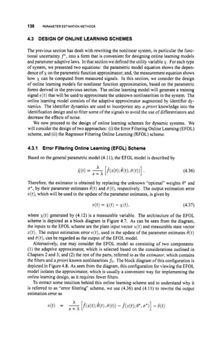
![146 PARAMETER ESTIMATIONMETHODS
and the EFOL scheme is described by
k(t) =
The same procedure followed earlier
(4.56)
X
S + X
for the case of a scalar parameter, can be applied
again here.. The main difference is that, since 8(t)is now a vecior, the Lyapunov function
candidate is
v(e,
8)= &e2 +eTr-le (4.57)
where r is a positive definite matrix that will ultimately appear in the adaptive law for
updating e(t)as the learning rate or adaptive gain. Using the same procedure as for the
scalar case we obtain the following parameter adaptive law:
e(t)= -r$(z)e. (4.58)
The details are left for the reader, as Exercise 4.7. In general, the adaptive gain r is a
positive-definite (symmetric) matri?. In many applications, it is simplified to r = 71,
which implies that each element e,(t) of the parameter estimate vector uses the same
adaptive gain. Another useful special case is that of a diagonal adaptive gain
In this case, each element &(t)of the parameter estimate vector has its own adaptive gain
yi,but there is no coupling between them.
Next, let us consider the case of a general filter W s instead of the first-order fil-
ter A*.From the parametric model ~ ( t )
= W(s)[O*$
(
.
)
I and it's estimate k(t) =
W(s)[BT$(t)],
we obtain that for S = 0 the output error e(t)= k(t)- X ( t ) satisfies
e(t) = ~ ( s ) [ B ~ $ ( z ) l .
We assume that the filter W ( s )= C(s1- A)-lB is SPR where (A, B, C) is a minimal
state-space realization of W(s).
The state-space model is
$ )
(4.59)
where eo is the state variable of the realization. Note that (4.59) is a theoretical tool that
supports the following analysis. The error e is still computed using (4.41).
To apply the Lyapunov synthesis method we select the Lyapunov function
where P > 0 is a positive definite matrix. The time derivative of V along the solutions of
(4.59) satisfies
V = E e i (ATP+PA) eo +,uP$(z)BTPeo+8Tr-G.
2](https://image.slidesharecdn.com/adaptive-approximation-based-controlcompress-230219164415-f6eb4a64/85/adaptive-approximation-based-control_compress-pdf-164-320.jpg)
![CONTINUOUS-TIME
PARAMETER ESTIMATION 147
Now, using the Kalman-Yakubovich-Popov Lemma (see page 392), since W ( s )is SPR
there exist positive definite matrices P, Q such that ATP +P A = -Q and B T P = C.
Therefore
V = -EeT Qeo +,dT$(z)Ceo +eTr-'e
2
2
-
- -Ee:Qeo +BTr-l
(4 +pr$(z)e) ,
which leads to the parameter adaptive law
8 = -pr+(z)e.
The reader will notice that this adaptive law is exactly of the same form as (4.58), even
though the filter W(s)is different.
4.4.1.3 LyapunovSynthesis Method forNonlinearly Parameterized Systems.
Now, we consider the case of nonlinearly parameterized approximators. The parametric
model (4.11) is given by
(4.60)
x
X(t)= s+x [m
e', .*)I I
and the EFOL scheme is described by
(4.61)
We attempt to follow a similar procedure as for the case of linearly parameterized approx-
imators. In this case, the output estimation error e(t) = g(t)- X(t)satisfies
x
S + X
e(t) = -"f*(z(t); 8,a)- f^(z(t);
o*,a*)],
which can also be written in state-space form as follows:
i. = -xe +x (j(z(t);
6,6)
- j ( z ( t ) ;
.o*,u*)).
Following the formulation of Chapter 2, f is assumed to be of the form
j ( ~ ;
e,.
) = $(z,~ ) ~ e .
Using the Taylor series expansion
where 8 = 6 - 8*, 5 = 6- u* are the parameter estimation errors and 3is a term that
contains the higher-order components of the Taylor series expansion. If these higher-order
terms are ignored for the purpose of deriving adaptive laws for e(t)and &(t),
we obtain](https://image.slidesharecdn.com/adaptive-approximation-based-controlcompress-230219164415-f6eb4a64/85/adaptive-approximation-based-control_compress-pdf-165-320.jpg)
![150 PARAMETER ESTIMATIONMETHODS
issue of persistency of excitation (see Section 4.5.4), which requires the regressor to
change sufficiently over any time interval in order for the parameter estimate vector
O(t) to converge to its true vector value 8'.
The third term, e(t),is the measurable output estimation error. This can be viewed
as the feedback information for the learning scheme. If the error e(t)is non-zero, it
provides two key pieces of information to the learning system: (i) the sign of e(t)
indicates to the learning scheme the direction in which the parameter estimate vector
should be changed to enhance learning; (ii) the magnitude of e(t) indicates to the
learning scheme by how much to update: large errors require larger modifications,
while small errors require only smallmodifications intheweights oftheapproximator.
If for some period of time t E [to, tl]the error e(t) x 0, where (tl - to) > X
this implies that the learning system already knows (or has already learned) this
information (contained in the parameter subspace spanned by the regressor ((t)for
t E [to, tl])and therefore there is no need to make any modifications to the value
of its parameter estimate vector during this time period. If we use the analogy of
classroom teaching, if the professor lectures on material that the students are already
familiar with, there is no learning taking place (surprise, surprise!).
The adaptive law described by (4.65) can be generalized to the case where the scalar
adaptive gain y is replaced by a positive definite matrix r of dimension qe-by-qe, where qe
is the dimension of 6'(t).This is achieved by re-scaling the optimization problem [157]. In
this case, the adaptive law becomes
The normalized gradient algorithm is a variation of the gradient algorithm, which is
sometimes used to improve the stability and convergence properties of the algorithm. The
normalized gradient algorithm is described by
(4.67)
where /3 2 0 is a design constant. If /3 is set to zero, the we obtain the standard (non-
normalized) gradient adaptive law.
The stability properties of the gradient algorithm are discussed in Section 4.5.2, while
the non-ideal case of b(t)# 0 and the derivation of robust learning algorithms are examined
in more detail in Section 4.6.
In this section we focused on an instantaneous cost function of a simple quadratic form.
The parameter estimation literature also contains some more advanced gradient algorithms
which are based on more complex cost functions. One such cost function that has attracted
some attention is the integral cost function of the form
The application of the gradient method to this cost function yields a new adaptive law whose
stability properties have been investigated in [119, 1381.
4.4.2.2 Least Squares Algorithms. Least squares methods havebeen widely used
in parameter estimation both in batch (nonrecursive) and in recursive form [I1, 1191. The](https://image.slidesharecdn.com/adaptive-approximation-based-controlcompress-230219164415-f6eb4a64/85/adaptive-approximation-based-control_compress-pdf-168-320.jpg)
![CONTINUOUS-TIME PARAMETER ESTIMATION 151
basic idea behind the least squares method is to fit a mathematical model to a sequence
of observed data by minimizing the sum of the squares of the difference between the
observed and computed data. To illustrate the least squares method, consider the problem
of computing the parameter vector 6’ at time t that minimizes the cost function
(4.68)
where ~ ( r )
is the measured data at time T , and ((7) is the filtered regressor vector at time
7 . The above cost function penalizes all the past errors C ( ~ ) ~ e ( t )
-~ ( r )
for 7 E [O,t].By
setting the gradient (with respect to 8)of the cost hnction to zero (VJ(8)= 0), we obtain
the least squares estimate for 8(t):
(4.69)
provided that the inverseexists. Thevalidity of this assumption is determined by the level of
regressor excitation. In the above formulation, we have considered the general case where
~ ( t )
is a vector (say of dimension m),which implies that O(t)is a matrix of dimension
qe-by-m.
The least squares estimate given by (4.69) is derived for batch processing; in other
words, all the data in the time interval [0, t]is gathered before it is processed. In adaptive
approximation, the estimated parameter vector 8(t)needs to be computed in real-time, as
new dara becomes available. The recursive version of the least squares algorithm for the
vector 6’ is given by
where P(t)is a square matrix of the same dimension as the parameter estimate @t).The
initial condition POof the P matrix is chosen to be positive-definite. In applications where
the measurements are corrupted by noise, the least squares algorithm can be derived within
a stochastic framework. In such a derivation, the matrix P represents the covariance of the
parameter estimation error. In deterministic analysis, even though this interpretation is not
applicable, P is often referred to as the covariancematrix.
It is interesting to note that the update law for 19,described by (4.70), is similar to the
gradient learning algorithm (4.66), with P(t)representing a time-varying learning rate. In
practice, recursive least squares can converge considerably faster than the gradient algo-
rithm at the expense of the increased computation required to compute P. However, in its
“pure” form the recursive least squares may result in the covariance matrix P(t)becoming
arbitrarily small. This problem, which is referred to as the covariance wind-up problem,
can slow down adaptation in some directions and, as a result, critically dampen the ability
of the algorithm to track time-varying parameters.
Several modifications to the ”pure” least squares algorithm have been considered. One
such modification is covariance resetting according to which the covariance matrix is reset
to P(tr)= POat time t, if the minimum eigenvalue of P(t,) is less then a predefined
small positive constant. This modification helps in preventing the covariance matrix from
becoming too small, but may result in large estimation transients immediately following
t = t,. A second commonly used modification to the least squares algorithm leads to the](https://image.slidesharecdn.com/adaptive-approximation-based-controlcompress-230219164415-f6eb4a64/85/adaptive-approximation-based-control_compress-pdf-169-320.jpg)
![152 PARAMETER ESTIMATION METHODS
least squares withforgettingfactor, which is given by
where p > 0 is typically a small positive constant, referred to as the forgetting factor. The
extra term pP(t)in (4.73) prevents the covariance matrix from becoming too small, but it
may, on the other hand, cause it to become too large. To avoid this complication, P(t)is
either reset to POor adaptation is disabled (i.e., P(t)= 0) in the case that P(t)becomes
too large. The literature on parameter estimation and adaptive control has several rules of
thumb on how to choose the design variables that appear in the least squares algorithm and
its various modified versions [119]. The stability and convergence properties of the least
squares algorithm are presented in Section 4.5.3.
4.4.2.3 Error Backpropagation Algorithm The error backpropagation algorithm
(orsimply backpropagation algorithm)isalearningmethod that hasbeen studiedandapplied
extensively in the neural networks literature. It appears that the term backpropagationwas
first used around 1985 [227]and became popular with the publication ofthe seminal edited
book by Rumelhart and McClelland [226]. However, the backpropagation algorithm was
discovered independently by two other researchers at about the same time [145,1941.After
the error backpropagation algorithm became popular, it was found out that the algorithm
had also been described earlier by Werbos in his doctoral thesis in 1974 [291]. Moreover,
the basic idea behind the backpropagation algorithm can be traced even further back to the
control theory literature, and specifically the book by Bryson and Ho [33].
In hindsight, it is not surprising that the error backpropagation algorithm was indepen-
dently discovered by somany researchers overthe years, since it is based on the well-known
steepest descent method, as it applies to the multi-layer perceptron. In this subsection, we
will describe briefly the error backpropagation algorithm for the training of multi-layer
perceptrons and we will relate it to the other learning algorithms that we developed in this
chapter.
The error backpropagation algorithm is derived by using the steepest descent optimiza-
tion method on the multi-layer perceptron. It provides a computationally efficient method
for training multi-layer perceptrons dueto the fact that it can be implemented in a distributed
manner. Moreover, the derivation of the local gradient for each network weight (parame-
ter) can be computed by propagating the error through the network in reverse; i.e., in the
opposite direction of processing the input signal. This is the reason for being called error
backpropagation algorithm. In contrast to the other learning algorithms developed in this
chapter for adaptive approximation of dynamic systems, the backpropagation development
herein is based on supervised learning for static systems.
The multi-layer perceptron was described in Section 3.6. The input-output ( z H y)
relationship of a multi-layer perceptron with n inputs, a single output, and one hidden layer
with qe nodes is given by](https://image.slidesharecdn.com/adaptive-approximation-based-controlcompress-230219164415-f6eb4a64/85/adaptive-approximation-based-control_compress-pdf-170-320.jpg)
![154 PARAMETER ESTIMATION METHODS
can be used indirectly, as a component of the adaptive law, in the computation of the partial
derivative if the multi-layer perceptron is used as the adaptive approximator.
Furthermore, it is worth noting that the concept of the error backpropagation algorithm
has also been extended to dynamical systems using learning algorithms such as dynamic
backpropagation [1811 and backpropagation through time [292], although the stability
properties of these algorithms are not established. One of the difficulties associated with
dynamic backpropagation type of algorithms is the fact it yields adaptive laws that typically
require the sensitivity of the output with respect to variations in the unknown parameters Q*.
Since these sensitivity functions are not available, implementation of such adaptive laws
is not possible and instead the designer needs to use an approximation of the sensitivity
functions instead of the actual ones. Onetype of approximation used in dynamic backprop-
agation is to replace the gradient with respect to the unknown parameters by the gradient
with respect to the estimated parameters. Such adaptive laws were used extensively in the
early neural control literature, and simulations indicated that they performed well under
certain conditions. Unfortunately, with approximate sensitivity functions, it is not possible,
in general, to prove stability and convergence. It is interesting to note that approximate
sensitivity function approaches also appeared in the early days of adaptive linear control,
in the form of the so-called MIT rule [1241.
4.4.3 Summary
In the previous sections we have developed a number of learning schemes. At this time, the
reader maybe overwhelmed by the differentpossible combinations. For example, one could
employ the error filtering scheme or the regressor filtering scheme; in the derivation of the
update law, there is the option of using a the Lyapunov synthesis method or optimization
approaches such as the gradient and the recursive least squares. Moreover, there are options
in selectingthe filter: aswe discussed, one could proceed with a first-order filter ofthe form
&or a more complicated filter W(s).There is also the selection of the approximator,
which can be linearly or nonlinearly parameterized. Lastly, within each selection there
are a number of design constants that need to be selected. In this subsection, we attempt
to put some order in the design of learning schemes by tabulating some of the different
schemes. The reader can obtain a better understanding of the issues by simulating the
learning schemes and varying some of the design variables.
Table4.1 summarizes the design options for the Error Filtering Online Learning (EFOL)
scheme. The stability properties of this approach are summarized in Theorem 4.5.1.
Table 4.2 summarizes the design options for the Regressor Filtering Online Learning
(RFOL) scheme, which is only applicable for LIP approximators. The stability properties
of this approach are summarized in Theorems 4.5.2 and 4.5.3.
4.5 ONLINE LEARNING:ANALYSIS
The previous three sections have introduced the idea of designing parametric models, learn-
ing schemes, and parameter estimation algorithms; the overall adaptive approximation
scheme was presented with a minimum of formal analysis. In this section, we examine
the stability and convergence properties of the developed learning schemes. In addition to
obtaining guarantees about the performance of the learning scheme, this stability analysis
provides valuable intuition about the underlying properties of the online learning methods
and in the selection of the design variables. The formal analysis of this section only consid-](https://image.slidesharecdn.com/adaptive-approximation-based-controlcompress-230219164415-f6eb4a64/85/adaptive-approximation-based-control_compress-pdf-172-320.jpg)
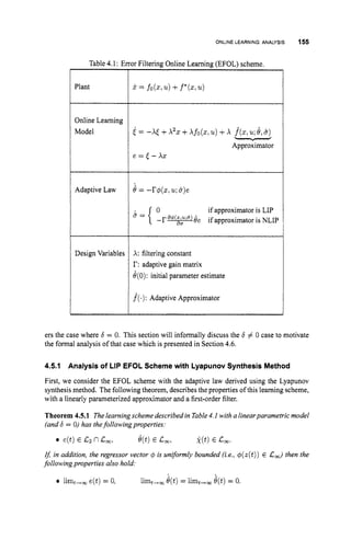
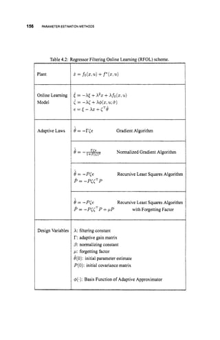
![ONLINE LEARNING: ANALYSIS 157
Proof: Based on (4.55) and (4.56), the output estimation error e(t) = k(t)-X ( t ) satisfies
the differential equation
~ ( t )
= -xe(t) +xeT(t)+(z(t)). (4.74)
Consider the Lyapunov function candidate
(4.75)
I p 2 p-T -1-
V(e,e) = -e +-0 r 0
2x 2
where p is a positive constant. By taking the time derivative of V along the differential
equations (4.74) and (4.58), and using the fact that 8' is constant we obtain
(4.76)
We are now in a position to utilize Lemma A.3.1 to show that e(t) E Cz,limt,, e(t) = 0,
e(t) E C
, and e(t)E C,. Moreover, since 0' is a finite constant, d(t)= &t)+0* is
also uniformly bounded (i.e., e(t)E C
,
)
. Finally, since @t)= r@e,with 6 E C
, and
Ifthe first-order filter &is replaced by a general filter W(s),
which is Strictly Positive
Real (SPR), then it is possible to obtain similar results. The details of the proof for an SPR
filter is left as an exercise (see Exercise 4.7).
e(t) -+ 0, it can be readily seen that limt+, 0(t)= limt+, e(t)= 0.
Effect of model error. In the case where 6 # 0, the error dynamics of eqn. (4.74) become
i(t)= -Xe(t) +xeT(t)+(z(t) - Xef, (4.77)
where the relation between 6and ef is given by
Therefore, the derivative of the same Lyapunov function becomes
V = -Fez -pefe (4.78)
which is not negative definite. Note that
v 5 -pleI (lel - kfl)' (4.79)
Therefore, V is only guaranteed to be negative semidefinite when /el 2 /efl. When
/el < /ef/,the Lyapunov function may increase. In fact, there is no bound on lleli while
lei < lef1. Let (tl,t2) denote a time period for which ]el < jef/. In this time period, it is
possible for llellto grow large, while maintaining 6(t)Tq5(z(t))=0. Ifat t = t2, the vector
+(z(t))
changes significantly dueto changes in z(t),then e(t,)Tq5(z(t,)) can become large
which causes lei to become large. Therefore, even if it is known that lef(t)l 5 5 for all
t > 0, where 5 is a small positive constant, it is not valid to state that ie(t)l is ultimately
bounded by /FI.
Therefore, in the presence of noise, disturbances, or modeling errors that can be rep-
resented by ef, there are no guaranteed stability or performance properties. Appropriate
robust methods to recover these properties will be discussed in Section 4.6.](https://image.slidesharecdn.com/adaptive-approximation-based-controlcompress-230219164415-f6eb4a64/85/adaptive-approximation-based-control_compress-pdf-175-320.jpg)
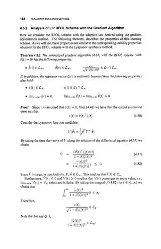
![ONLINE LEARNING:ANALYSIS 159
therefore, since 8 E C
, we obtain
This implies
Moreover,
Therefore, we obtain that 8 E C,.
e(t)TC(t)E C
, and e(t)E C2 nC
,
. Next, consider the error derivative
Now, if we assume that ((t)is uniformly bounded, we can easily obtain that a(t)=
C ( t ) = B(t)TC(t)+6(t)T((t)
Using the normalized adaptive law for e(t)and the fact that e(t),[(t)E C
,
, we obtain
8 E 1
3
,
. Moreover, since C(t)= W(s)[$(t(t))]
is the output of a stable SPR filter W(s).
with a bounded input $, we obtain that 5 E C,. Therefore, C E C
,
. Since e E C2 nC
,
and d E Co3,using Barbilat's Lemma we conclude that limt,, e(t) = 0. Moreover, it
W
It is important to note that even in the restrictive case of no approximation errors and a
linearlyhparameterized approximator, it cannot be established that the parameter estimate
vector O(t)will converge to the optimal vector O*. To guarantee that O(t) will converge to
O', the regressor vector C(t)needs to satisfy a so-calledpersistency o
f excitation condition.
Intuitively,this impliesthat there should be sufficientvariation in [(t)
to allowthe parameter
estimates to converge to their optimal values. The concept of persistency of excitation is
discussed in Section 4.5.4.
can be readily seen that limt,, O(t)= limt,, O(t)= 0.
Effect of model error. In the presence of approximation errors (i.e., b(t) # 0), the eqn.
(4.80)
becomes
e(t)= @ t ) T ~ ( t )
- 6(t).
Therefore, the derivative of the Lyapunov hnction becomes
(4.83)
This is only negative semidefinite if e(t)2> -b(t)e(t) for all t. Even if b(t)is known to be
upper bounded, this condition cannot be guaranteed for small e(t).Therefore, the stability
of the gradient algorithm (4.66)
cannot be guaranteed. In fact, it is known from adaptive
parameter estimation of linear systems that even if b(t)is a small signal it can be sufficient
to make the adaptive system unstable. The instability is typically caused by drift of the
adaptive parameter estimates. To address this problem, the standard update law described
by (4.66)
needs to be modified. Several modifications exist in the literature for enhancing
the robustness of adaptive schemes. These modifications are discussed in Section 4.6.](https://image.slidesharecdn.com/adaptive-approximation-based-controlcompress-230219164415-f6eb4a64/85/adaptive-approximation-based-control_compress-pdf-177-320.jpg)
![ONLINE LEARNING: ANALYSIS 161
= -e2+;0l - T CCT -
O
This implies V E C
, and e E L2. If ((t)is uniformly bounded then e E C,. Using a
similar procedure as in the stability proof of the gradient algorithm, we obtain that e E C,.
In comparing the stability properties of the gradient and least squares algorithms we no-
tice that in addition to the other boundedness and convergence properties, the recursive least
squares also guarantees that the parameter estimate 6(t)converges to a constant vector e.
If the regressor vector Csatisfies the persistency of excitation condition then 6(t)converges
to the optimal parameter vector 8'.
Despite its fast convergenceproperties, the recursive least squaresalgorithm has not been
widely used in problems involving large function approximation structures, mainly due to
itsheavy computational demands. Specifically,ifthe number of adjustable parameters is N ,
then updating of the covariance matrix P(t)requires adaptation of N 2 parameters. Issues
related to least-squares-based learning and its computational requirements are discussed
in some detail in Exercise 4.4. An alternative locally weighted learning approach that
can have considerably smaller computational requirements, referred to as receptive jeld
weightedregression [13,236,237], is discussed in Exercise 4.5.
Effect of model error. When 6(t) # 0, then e(t) = t?(t)T<(t)
- 6(t). Therefore, the
derivative of the Lyapunov function becomes
Therefore, using Barbillat's Lemma we conclude that lirnt+= e(t)= 0.
= -(e +6)e +s ( e
1 +6)2
Therefore, V is negative semidefinite only if le(t)l > I6(t)l for all t. Once le(t)l becomes
smaller than lb(t)1 then the derivative becomes positive.
4.5.4 Persistencyof Excitationand ParameterConvergence
In Section4.5itwas established that under certain conditions theparameter estimatesremain
bounded and the output estimation error convergesto zero asymptotically. We also saw that
the various adaptive approximation schemes presented in this section could not establish
that the parameter estimation vector e(t)will converge to the optimal parameter vector O',
even in the special case of linearly parameterized approximators with no approximation
error (6(t)= 0).
The observation that it is pos!ible for the output error e = y - 9 to be zero while the
parameter estimation error 6 = 8 - O* is non-zero was also made in Example 4.1for the](https://image.slidesharecdn.com/adaptive-approximation-based-controlcompress-230219164415-f6eb4a64/85/adaptive-approximation-based-control_compress-pdf-179-320.jpg)
![162 PARAMETERESTIMATION METHODS
linear case and in Example 4.2 for the nonlinear case, where forAcertaininputs the output
estimation error e(t)+ 0, while the parameter estimate 6(t)+ 6, # 6’.
In this subsection, we consider the issue of parameter-convergence, and present condi-
tions under which the parameter estimation error 6(t)= 0 -0”converges to zero. Conver-
gence conditions are related to the issue of persistency of excitation, which is an important
topic when the objective is to achieve parameter convergence. In adaptive approximation
based control the objective typically is to track a desired signal, not to achieve convergence
of the parameter estimation error.
To extract some intuition behind persistency of excitation and parameter convergence,
let us consider the gradient algorithm within the RFOL scheme. In this case, the parameter
update law and output estimation error e(t)satisfy
. .
8 = 8 = -r((t)e(t):and
e(t) = ~ ( t ) ~ 8 .
From (4.85H4.86)we obtain
8= -r((t)C(t)T8.
(4.85)
(4.86)
(4.87)
As longasthe adaptive gainmatrix r is positive definite, itdoesnot play arole in whether the
parameter estimation error converges to zero or not, but it does influence (significantly) the
rate of convergence. Therefore, we note that the convergence of the parameter estimation
error 8(t)depends on the matrix C(t)C(t)T.
In general, for parameter convergence it is desired that ((t)C(t)Tstays away from zero
in some sense -this is exactly the concept that the persistency of excitation condition
formalizes.
Definition 4.5.1 A bounded vector signal 5 E Peis persistently exciting (PE) i
f there
exists o > 0 and 6 > 0 such that
for all t 2 0.
We note that at any time instance t the qe x qe matrix C(t)C(t)Thas rank 1. Therefore, the
PE condition is not expected to hold instantaneously, but the idea is that over every time
period [t, t +61 the integral of ((t)C(t)T
retains a rank equal to 40.
It canbe shown [138,2351that if( ( t )isPE andpiecewise continuousthen the equilibrium
8= 0 of the differential equation (4.87) is globally exponentially stable.
It is recalled that the filtered regressor vector ( ( t )is obtained by filtering the regressor
4; that is,
Therefore, the condition of PE on C is influenced, in general, by the signals u(t),s(t),
and also possibly by the filter W(s).Since z(t)is the output of the system with u(t)as
input, we see that the unknown system also influences the PE condition on ((t).For the
special case of a linear system, with the unknown parameters 6* being the coefficients of
the numerator and denominator polynomial of the transfer function, it can be shown that
the persistency of excitation condition on ( ( t )can be converted to a “richness” condition
[119] on the input u(t).Specifically, under such conditions, ((t)is PE if u(t)has at least
290 frequencies [235]. In this case, u(t)is said to be suficiently rich.
The above results show the relationship between the PE condition and parameter conver-
gence. Although the above formulation has considered the RFOL scheme with the gradient
C(t)= W S ) 1
4( 4 t h 4t))l ’](https://image.slidesharecdn.com/adaptive-approximation-based-controlcompress-230219164415-f6eb4a64/85/adaptive-approximation-based-control_compress-pdf-180-320.jpg)
![ROBUSTLEARNINGALGORITHMS 163
algorithm, similar results can be obtained for the RLSalgorithm aswell as the error filtering
scheme. For a detailed treatment of parameter convergence in various linear identification
schemes, the interested reader is referred to [119, 179,2351.
Subsequent chapters will focus on the problem of designing approximation based track-
ing controllers for nonlinear systems. In such tracking control applications, a goal is to force
the system state vector z(t)to converge to a desired state vector xc(t).The control input
u(t)is determined by the history of x(t),zc(t),and the error between them. Assuming
that the controller is able to achieve its goal of forcing E = z - x, toward zero, then the
reference trajectory xc plays a very significant role in determining whether q5 and hence (
satisfy the persistence of excitation condition.
For local basis elements, especially radial basis functions, various authors have consid-
ered the issue of persistence of excitation in adaptive approximation types of applications,
e.g., [74,75, 100, 141,2331. The problem is particularly interesting with locally supported
basis elements. For example, the results in [loo, 1411 demonstrate that persistence of ex-
citation of the vector @ is achieved if for a specified E > 0 there exists T > ,
u > 0 such that
in every time interval of length T the state x spends at least p seconds within an E neighbor-
hood of each radial basis function center. Note that since the centers are distributed across
the operating region 'D, this type of condition would require the state (and the commanded
trajectory 5,) to fully explore the operating region in each time interval of length T . This
is impractical in many control applications, but is required if the objective is to achieve
convergence of the parameters over the entire region D.
If SI, denotes the support of the k-th element of 4 and each SI, is small relative to 'D
(e.g., splines that become zero instead of Gaussian RBFs that approach zero asymptoti-
cally), then the results in [74,75] present local persistence of excitation results that ensure
convergence of the approximator parameters associated with @I, while x E SI,. These local
persistence of excitation results are very reasonable to achieve in applications, but approx-
imator convergence is only obtained in those regions SI, that lie along the state trajectory
corresponding to x,.
4.6 ROBUST LEARNINGALGORITHMS
The learning algorithms designed by the procedure described in Sections 4 2 4 4 . 4 , and
analyzed in Section 4.5 are based on the assumption that b = 0. In other words, it was
assumed that the only uncertainty in the dynamical system is due to the unknown f *(x,
u),
which can be represented exactly by an adaptive approximation function f(z,
u;
B*, a*)
for some unknown parameter vectors B* and CT*. In practice, the adaptive approximation
functionf(x: u;
B*, u * )maynotbeabletomatchexactlythemodelinguncertaintyf*(x,u),
even if it was possible to select the parameter vectors 8 and b optimally. This discrepancy
is what we defined as "minimum functional approximation error" (MFAE) in Section 3.1.3
and Section 4.2.
In addition to the MFAE, there are other types of modeling errors that may occur:
Unmodeled dynamics. The dimension of the state space model described by (4.5)
may be less than the dimension of the real system. It is quite typical in practice
to utilize reduced order models. This may be done either purposefully, in order to
reduce the complexity of the model, or due to unknown dynamics of the full-order
model. Indeed, in some applications (such as in flexible structures) the full-order
model may be of infinite dimension.](https://image.slidesharecdn.com/adaptive-approximation-based-controlcompress-230219164415-f6eb4a64/85/adaptive-approximation-based-control_compress-pdf-181-320.jpg)
![ROBUST LEARNING ALGORITHMS 165
4.6.1 ProjectionModification
One of the most straightforward and effective ways to prevent parameter drift is to restrain
the parameter estimateswithin apredefinedbounded andconvex region S,which isdesigned
to ensure that 8
' E S.In addition, the initial conditions 8(0)are chosen such that e(0)E 5.
The projection modification implements this idea as follows: ifthe parameter estimate 8(t)
is inside the desired region S,or is on the boundary (denoted by bS)with its direction of
change toward the insidethe region S,then the standard adaptive law (4.88) is implemented.
In the case that 8(t)is on the boundary 6
sand its derivative is directed outside the region,
then the derivativeis projected ontothe hyperplane tangent to 6
s
.
Therefore, the projection
modification keeps the parameter estimation vector within the desired convex region S for
all time.
Next, we make the projection modification more precise. Let the desirable region S be
a closed convex set with a smooth boundary defined by
s = (
8E 1 K ( e ) 5 0
)
where K : P o H $2 is a smooth function. According to the projection algorithm, the
standard adaptive law (4.88) is modified as follows:
if8 E SOor if
8 E bS and VnTr(E 2 0 (4.89)
i-I?& +r:;F:KI-'<& otherwise
e(t)= p[-rtE]
=
where Sois the interior of S,6
sis the boundary of S,and VK= f .
To illustrate the use of the projection algorithm, we now consider some examples.
EXAMPLE4.9
Consider a desirable region S defined by all the values of 8 E !
I
F that satisfy eT8 5
M 2where M isapositive constant. Inthis case, theparameter estimates areprevented
from becoming too large by restricting them within the region 0'8 5 M2. By
defining ~ ( 8 )
= eT8 - M2,we obtain the column vector VK= 28. Therefore, the
projection algorithm (4.89) becomes
ifil81iz< M
or if l18ii2= M and eTI'<& _> 0 (4.90)
-r@+I'&r@ otherwise.
8Tri
A
The above modification guarantees that l18(t)1l2 5 M for all t 2 0 as long as
ll~(o)llz5 M .
EXAMPLE 4.10
Now consider a two-dimensional parameter estimate8 = (81 &IT, where it is known
that el 5 8, 5 elande25 82 5 3 2 . The lower and upper limits e,,~
9
, and8 1 , 8 2 are
assumed to be known. Therefore, in this case the desirable region Sis a rectangle. For
simplicity,let us choose the learning rate matrix tobe diagonal; i.e., I' = diag(y1,y~).](https://image.slidesharecdn.com/adaptive-approximation-based-controlcompress-230219164415-f6eb4a64/85/adaptive-approximation-based-control_compress-pdf-183-320.jpg)
![ROBUST LEARNING ALGORITHMS 167
only make the Lyapunov function derivative more negative, the stability properties derived
rn
Remark: In the above proof, we use the following standard result from vector calculus:
for two vectors a,b E %Iz", if aTb > 0 then the angle between the two vectors is less than
90". If aTb = 0 then the two vectors are orthonormal, and the angle between them is 90".
for the standard algorithm still hold.
Effect of Model Error. Note that the projection operator has no effect on the parameter
estimation as long as 0 E S.Therefore, in the case where 6 # 0, the projec:ion method
does not prevent an increase in the Lyapunov function (i.e., an increase in Ilellr) when e
is small relative to 6. The projection operator only prevents 6 from leaving S. Therefore,
use of the projection method does not guarantee a small ultimate bound on e(t)in the case
where 6 # 0. Consider the following example which extends the EOFL analysis that is on
page 144.
EXAMPLE 4.11
In this example, we will let 6(t)= [E] where ~ ( t )
is the combined modeling errors
due to disturbances, MFAE, etc. that add into the j
.equation. The EOFL learning
system variables are defined as
x = [(s*)T4 +6, 2 = S+X [ e ~ ] e(t)= P [ - ~ E E ]
e = k - x , e=e-e*.
- A
Therefore,
d = -xe +xeT$- AE.
Consider the Lyapunov function V of eqn. (4.75). The time derivative of V using
the projection form of parameter adaptation is
= -pe2 - pee +peTrW1Q
where Q is defined in (4.93). On the interior of S,Q = 0; therefore,
2
V = -pe -pee.
Even if E is bounded as Ie/ < 5, the term ee is sign indefinite. Using the upper bound,
v < -Pbl (lel - 5)
we can show that that V will decrease for /el > 5; however, when /el < 5 it is
possible that V will increase until 0 E 6
s
.
Figure 4.11 shows the type of trajectory
that could occur. In this figure, the parameter error and e decrease until lei < 5. Once
that inequality is satisfied, the parameter error diverges until 0 E 6
s
.Eventually
e increases. Once /el > 5, the Lyapunov function again decreases. Note that such
behavior could occur repetitively. n](https://image.slidesharecdn.com/adaptive-approximation-based-controlcompress-230219164415-f6eb4a64/85/adaptive-approximation-based-control_compress-pdf-185-320.jpg)
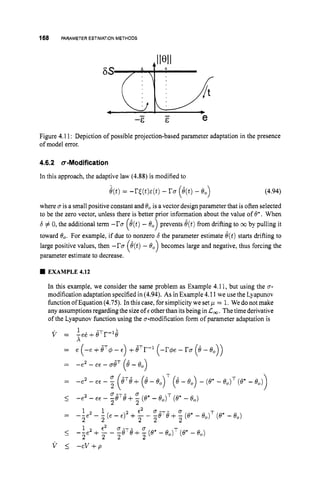
![170 PARAMETERESTIMATIONMETHODS
v 5 - c v + p
where
Therefore, we obtain similar results as with the u-modification.
4.6.4 Dead-ZoneModification
When 6 = &[E] # 0 (e.g., in the presence of approximation errors), the adaptive law
(4.88) tries to drive the estimation error E to zero, sometimes at the expense of increasing
the magnitude of the parameter estimates. The idea behind the dead-zone modification
is to enhance robustness by turning off adaptation when the estimation error becomes
relatively small compared to E. Note, for example, that in eqn. (4.79)the time derivative
of the Lyapunov function is negative semidefinite for
the Lyapunov function is decreasing. When I E ~ < /el, then the parameter estimates may
diverge and the Lyapunov function may increase. The apparently simple solution is to stop
parameter estimation when I E ~ < lei.
> /EI. Therefore, for I E ~ >
The dead-zone modification is given by
(4.96)
where €0 is a positive design constant intended to be an upper bound on E ( t ) . One of the
drawbacks of the dead-zone modification is that the designer needs an upper bound on the
model error, which is usually not available. Therefore, €0 must be selected conservatively
to ensurethat it overbounds E(t). A second drawback of the dead-zone approach is that even
in the case where E ( t ) = 0, asymptotic stability of the origin cannot be proved; instead,
uniform ultimate boundedness of the origin is attained with the size ofthebound determined
by €0 and the control parameters.
If ~ ( t )
> €0 for any interval of time for which l ~ l
< E, then the Lyapunov function may
increase. Note that the dead-zone approach can be combined with the other approaches
(e.g., projection). Such combined approaches are considered further in the example at the
end of this section.
EXAMPLE 4.13
In this example, we consider the same problem as Example 4.11, but using the dead-
zone adaptation specified in eqn. (4.96). As in Example 4.1 1, we use the Lyapunov
function of eqn. (4.75)(with ,
u = 1)andwe assume that E < 5. The time derivative of
the Lyapunov function using the dead-zone form of parameter adaptation for /el > e0
is](https://image.slidesharecdn.com/adaptive-approximation-based-controlcompress-230219164415-f6eb4a64/85/adaptive-approximation-based-control_compress-pdf-188-320.jpg)
![ROBUST LEARNINGALGORITHMS 171
Figure 4.12: Depiction of possible dead-zone based parameter adaptation in the presence
of model error.
= e (-e +eT4-t) - BTr-l(r4e)
< -le/ (lei - 5)
= -e2 - ee
There are now two cases to consider €0 > 5 and €0 < 5. The designer of course will
try to select €0 > S, but since 5 may not be know it is important to understand the
consequences of haying €0 < 5.
If €0 > S
,then V < 0 whenever parameter adaptation is active (i.e., /el 2 €0).
When /el < €0, parameter adaptation stops. Note that if the trajectory enters the
dead-zone at time tl and leaves the dead-zone at time tz,then /e(tl)l = le(tz)/ = €0
and &t,) = e ( t 2 ) ; therefore, V(e(tl),e(t1)) = V(e(t2),e ( t 2 ) ) . If odd subscripted
times (i.e., t2%+1 for i = 1,2,...) denote times at which the trajectory leaves the
dead-zone and even subscripted times (i.e,, t2, for i = 1,2, ...) denote times at
which the trajectory enters the dead-zone, the? extension of the abov? argument
V(e(tz,),e ( t 2 , ) ) . In fact, ifwe denote a = €0 - S > 0 then outside the dead-zone
shows that V(e(t2%-1),
e(t2,-1)) = V(e(tz,),O(t2,)) and V(e(tn,+l),O(tz%+l))I
v < -€oa<O;
therefore, V(e(tzz+l),B(t2,+1)) 5 V(e(tz,), e ( t 2 , ) ) -~0a(t2,+1
-t2,). This shows
that the total time outside the dead-zone must satisfy the following inequality
where q may be finite or infinite, but the cumulative time outside the dead-zone is
finite [87]. Therefore, in this example, le(t)l is ultimately bounded by €0. Such a
possible trajectory is depicted in the left image of Figure 4.12.
If €0 < 5, then, even though parameter adaptation will stop for /el < €0, the
Lyapunov function and in particular the parameter estimation error may increase for
5 > (el > €0. Two possible trajectories are depicted in the image in the right half
of Figure 4.12. Note that while 5 > /el > €0 the Lyapunov function can increase
without bound. n](https://image.slidesharecdn.com/adaptive-approximation-based-controlcompress-230219164415-f6eb4a64/85/adaptive-approximation-based-control_compress-pdf-189-320.jpg)
![172 PARAMETERESTIMATION METHODS
4.6.5 Discussionand Comparison
In the presence ofmodel errors (i.e., b # 0),the aboverobust adaptive laws guarantee, under
certain conditions, that the parameter estimates O(t) and the estimation error ~ ( t )
remain
bounded. We haveincluded severalexamplesintheprevious subsectionstoclarify and allow
comparison between the bounds available from the alternative approaches. To be useful
as design tools, the designer should be able to clearly understand how to make the bound
smaller as a function of the approximation structure or the control and estimation design
parameters. Although, in the presence of approximation error, it cannot be established
that E ( t ) will converge to zero, it can be shown that the estimation error is small-in-the-
mean-squared sense [119], in the sense that integral square error over a finite interval is
proportional to the integral square approximation error (see Section A.2.2.4).
In the introduction to this section, we stated that there were two categories of approaches
for increasing the robustness of parameter adaptation methods to model error. As the
discussion ofthis sectionhas pointed out, the first category of methods (is., cr-modification,
€-modification, and projection) do not require any assumptions about upper bounds on the
model error and do prevent the parameter estimates from diverging to infinity, but also are
not guaranteed to maintain the accuracy of theparameter estimateswhen the training error is
small relative to the model error. The second category of methods (i.e., dead-zones) require
an assumption of a known bound on the model error. If this assumption is valid, then the
dead-zonemaintains the accuracy of the parameter estimate when the training error is small
relative to the modeling error. If the assumed size of the bound is invalid, then there are
no guarantees. Note that the best of both approaches is easily achievable by implementing
one of the approaches from each category.
EXAMPLE 4.14
In this example, we consider the same problem as Example 4.11, but using the pro-
jection and dead-zone adaptation:
(4.97)
where the projection operator is defined in eqn. (4.89) and the dead-zone is imple-
mented as
if E 2 €0
d ( E ) = { otherwise.
The analysis for this approach must consider a few cases. If the assumption that
5 < e0 is valid, then projection maintains t
9 E S while the dead-zone maintains the
accuracy oftheparameter estimate whenthe training erroris small; thus preventing the
possible divergence of the parameter estimate depicted in Figure 4.11. Alternatively,
if the assumption that 5 < €0 is not valid then projection would prevent divergence
to infinity as depicted in the right image of Figure 4.12 when 5 > lel > €0. In
both of these cases, performance of parameter estimation using both projection and
n
a dead-zone is better than using either approach alone.
Implementation of the dead-zone or projection methods as written would involved dis-
continuous differential equations. Therefore, implementations usually involve smoothing
of the discontinuities.](https://image.slidesharecdn.com/adaptive-approximation-based-controlcompress-230219164415-f6eb4a64/85/adaptive-approximation-based-control_compress-pdf-190-320.jpg)
![174 PARAMETER ESTIMATION METHODS
where f(z)
= OT4(x)+ep(x) with lef(z)l < E on V.Define
i = f*(z)+L(y-Y)
y = ?
where f(z) = 6'TI$(z).
Also, define e = z - 2 and 8 = 6' - 8. The above defines a
parametric model and learning scheme with training signal e that can be computed from
available signals.
1. Find the differential equation for e.
2. Use the Lyapunov candidate function V =
3. For the case that E = 0, prove the properties of e and 6.
4. For the case that E # 0, but an upper bound is known, what is the appropriate dead-
zone size to ensure uniform boundedness of the solution. What is the uniform bound
on je(t)l?
e2+8Tr-18 to derive a stable
( -)
parameter update law for the case that E = 0. What constraint is required for L?
Exercise 4.4 In this exercise, we consider the second order case where the system model
is
(4.98)
Y = 21 (4.99)
where y and u are available signals. In particular, the derivative of the output z2is not
directly measured. The functions f and g are not known and will be approximated. An
important aspect of this problem is that unknown nonlinearities f and g depend only on the
directly measurable signal y. If this approach is understood, then generalization to the n-th
order case is straightfonvard.
1. Assuming that f(y) = e;I$f(y) andg(y) = OJ&(y), show that the state differential
equation can be written as
2 2
[ s:] = [ OT@(y,u)]
where OT = [OT, 8:] E XZNand @(V>u) = @;I.
2. Add and subtract a121 T a221 to both sides of the equation
$1 = f b )+4 Y ) U
to show that
where
9 = QT@F +YFl $
. YF2
(4.100)](https://image.slidesharecdn.com/adaptive-approximation-based-controlcompress-230219164415-f6eb4a64/85/adaptive-approximation-based-control_compress-pdf-192-320.jpg)
![EXERCISESAND DESIGN PROBLEMS 175
Note that (s2+als +u2) = 0 must be a Hurwitz polynomial.
3. Let
Q = GT@F+yFl +yF*
and e = Q - y. Show that e = OT@p
where 6 = 6- 0.
4. Relative to the cost function
the adaptation algorithm for least squares with forgetting is:
P = - P @ F @ ~ P
+pP with P(0)positive definite
0 = -P@Fe.
(a) Show that the time derivative of the Lyapunov function V = 6TP-'6 is
V = - ( p V +e'). Show that V E Cm, V E Cz,and e E CZ.
(b) Show that implementation of the this least squares approach requires imple-
mentation of 2N +2 second-orderfilters plus solution of (4N2+2N) ordinary
differential equations.
5. Implement a simulation using f = 0, g = 2 +sin(y2), and
1
u = 1( - ~ 1 (y - 2 sin(rt))- ~2 -yFl - 2r cos(rt) +2 2 sin(rt)
2 (:: 1
The choice ofparameters K1 = 1,K2 = 1
,a1 = 3.5, a2 = 49, and p = 0.01works
reasonably well. Let f = 0 and g = O:$g(y) where #g is composed of Gaussian
radial basis functions defined by eqn. (3.23) with centers separated by y = 0.3and
uniformly covering y E 2
) = [-6,6]. Let the simulation run for at least 100 s.
(a) Since g is available in simulation, you can compute 09.Use this known vector
to plot the norm of the approximator parameter error as a function of time.
Discuss.
(b) Use the known value of 8, to plot the plot the value of the Lyapunov function
versus time. Discuss.
(c) Plot g and g (at least) at the beginning and end of the simulation. Discuss why
it is more accurate in some regions of '
D than others.
(d) Repeat the above simulation using alternative definitions of the approximator.
Be certain to try some approximator with globally supported basis functions.
Compare such items as the number of filters needed to compute @F and the
approximation accuracy.
6. In the above controller, fypl is used as an estimate for the unmeasured quantity
y = x2. Use Laplace anaiysis to show that this approximation is reasonable at low
frequencies (i.e., s near zero).
Note that in this approach P has row and column dimensions equal to q = dzm(O)= N
which canbe quite large, especially when the dimension of D is larger than one. A similarly](https://image.slidesharecdn.com/adaptive-approximation-based-controlcompress-230219164415-f6eb4a64/85/adaptive-approximation-based-control_compress-pdf-193-320.jpg)
![176 PARAMETERESTIMATIONMETHODS
large number offilters is required to compute @F. The computations required for this least
squares implementation can become impractical in some applications. For comparison, see
the approach of Exercise 4.5.
Exercise 4.5 This exercise considers an alternative estimation approach that is referred to
inthe literature asreceptive fieldweighted regression (RFWR) [236,237]. For convenience,
we will consider the sameapplication as Exercise 4.4,only the approximator andestimation
algorithms will change.
1. Assume that
The following items clarify the constraints assumed in this decomposition.
(a) { ~ k ( x ) } E ~
defines a set of continuous, positive, locally supported weighting
functions.
(b) = {z E I w k ( x ) # 0 ) denotes the support of w k ( x ) . The weighting
functions W k are defined so that each set s k is convex and connected and l
J =
u,"=,s k . An example of a weighting function satisfying the above conditions
is the biquadratic kernel defined as
where c k isthe center location ofthe k-th weighting function and pk isa constant
which represents the radius of the region of support.
(c) To simplify expressions used later, define
The set of non-negative functions {&(x)}tLl forms apartition o
f unity on V:
W k ( S ) = 1, for all x E v.
Note that the support OfLdk(z) is exactly the
same as the support of 3
1
,(x).
(d) On each region s k ,
f k ( x > e f k ) = 'd'A(x)ofk and g k ( x j B g k ) = ' d ' L k ( x ) e g k
are local estimates to f and g . Since each region s k is small, the local ap-
proximations can be quite simple. For example, an affine approximation such
as .fk(z, efk)= B +ofk.(x - C k ) would yield @fk = [I,(x- C k ) l T and
-P
* f k = P f k , , e f k , l .](https://image.slidesharecdn.com/adaptive-approximation-based-controlcompress-230219164415-f6eb4a64/85/adaptive-approximation-based-control_compress-pdf-194-320.jpg)
![EXERCISESAND DESIGN PROBLEMS 177
Under the assumption that, for y E s k it is true that f(y) = f k (y) and g(y) = gk(y),
show that the state differential equation of (4.98) can be written as
(4.105)
2. Add and subtract alj.1 +a251 to both sides of the equation
and y ~ ~ ,
y ~ ~ ,
and (s2 +als +a2) are as defined in Exercise 4.4.
3. Let
^ T
$k = @ k QFk +yF1 +!/Fz
and ek = yk - y. Show that ek = 6;*pk where 6, = 6, - 01;.
4. In contrast tothe least squarescost function of eqn. (4.1Ol), which allows cooperation
between all the elements of 0 in fitting the data over D,RFWR uses the locally
weighted error criterion:
t 2
J k ( @ k ) = 1e-'("-"~k(Y(.)) (Y(') - yk ( e k ( ~ ) . Q F ~ ( ' ) , y ~ l ( ' ) . Y F z ( ' ) ) )
dT
(4.106)
where all arguments indicated by (.) are (r)'sAthatwere eliminated to make the
equation fit on the line. In this approach, each @k is optimized independently over
Sk. The RFWR adaptation algorithm is:
& = - 3 k P k Q F Q : P k +a k / b p k with P k ( 0 ) positive definite
6 k = - 0 k P k Q F e k .
Note that both differential equations automatically turn off when y $ s k . Note also
that both forgetting and learning are localized to the regions s k corresponding to
active weighting functions.
(a) Show that the time derivative of the Lyapunov function v = EElv k with
v k = 6 l P L 1 6 k is
.I;I
v=-C[-
d k ( p v k +e i ) ]
k=l
where the term in square brackets is the vk. Showthat v,v k E c,, v k . v.e E](https://image.slidesharecdn.com/adaptive-approximation-based-controlcompress-230219164415-f6eb4a64/85/adaptive-approximation-based-control_compress-pdf-195-320.jpg)
![180 NONLINEARCONTROLARCHITECTURES
handle all nonlinearities within the assumed bound. As a result, they may result inhigh-gain
control algorithms. As we will see, one of the key motivations of adaptive approximation is
to reduce the need for such conservative control design. Finally, Section 5.5briefly presents
the adaptive nonlinear control methodology, which is based on the estimation of unknown
parameters in nonlinear systems.
Naturally, it is impossible to cover in a single chapter all nonlinear control design and
analysis methods. By necessity, many of the technical details have been omitted. An
excellent treatment of nonlinear systems and control methods is given in [134]. The intent
of the present chapter is to introduce selected nonlinear control methods, highlight some
methods that are robust to nonlinear model errors, and to motivate the use of adaptive
approximation in certain situations. Throughout this chapter, the main focus is on tracking
control problems, even though where convenient we also consider the regulation problem.
Also, the presentation focuses on systemswhere the full state is measured; output feedback
methods are not discussed.
5.1 SMALL-SIGNAL LINEARIZATION
Consider the nonlinear system
x = j(x,u)
where f(z,
u)is continuously differentiable in a domain Dz x D, C !Rn x W. First, we
consider the linearization around an equilibrium point x,,which for notational simplicity
is assumed to be the origin; i.e.,x = 0, u = 0. Then we consider the linearization around
a nominal trajectory x*(t).Finally, we describe the concept of gain scheduling, which is a
feedback control technique based on linearization around multiple operating points.
The main idea behind linearization is to approximate the nonlinear system in (5.1) by a
linear model of the form
x = A x +Bu
where A, B are matrices of dimension n x n and n x m,respectively. Typically, the linear
model is an accurate approximation to the nonlinear system only in a neighborhood of the
point around which the linearization took place. This is illustrated in Figure 5.1, which
depicts linearization around x = 0. As shown in the diagram, the linearized model Az
is a good approximation of f(z)
for z close to zero; however, if x(t)moves significantly
away from the equilibrium point z = 0, then the linear approximation is inaccurate. As a
consequence, a linear control law that was designed based on the linear approximation may
very well be unsuitable once the trajectory moves away from the equilibrium, possibly due
to modeling errors or disturbances.
The term small-signallinearization is used to characterize the fact that the linear model
is close to the real nonlinear system if the system trajectory x(t) remains close to the
equilibrium point x, or to the nominal trajectory x*(t). Therefore, for sufficiently small
signals z(t) - x,, the linearized system is an accurate approximation of the nonlinear
system. The term “small-signal” linearization also distinguishes this type of linearization
fromfeedback linearization, which will be studied in the next section.
In general, feedback control techniques based on the linear model work well when
applied to the nonlinear system if the uncertainty of the system is small, thus allowing the
feedback controller to keep the trajectory closeto the equilibriumpoint 5 , . Obviously, linear
controllers derived based on small-signal linearization have good closed-loop performance
in cases where the system nonlinearities are not dominant or they donot have a destabilizing](https://image.slidesharecdn.com/adaptive-approximation-based-controlcompress-230219164415-f6eb4a64/85/adaptive-approximation-based-control_compress-pdf-198-320.jpg)
![SMALL-SIGNAL LINEARIZATION 181
Figure 5.1: Diagram to illustrate small-signal linearization around x = 0.
effect. For example, stabilization of the origin, the nonlinearity of the scalar system
x = x - x3 + u
has a stabilizing effect, thus if the control law u = -22 isused then for the resulting closed-
loop system i = -z - x3 the origin is asymptotically stable even though the nonlinear
term -x3 has not been removed by the control law.
5.1.1 Linearizing Around an Equilibrium Point
If the nonlinear system of (5.1) is linearized around (2, u)= (0, 0) then the linear model
is described by
x = AX+Bu
where the matrices A E !Px"
and B E E
n
'
" are given by
(5.2)
(5.3)
If we assume that the pair (A, B ) is stabilizable [10, 19, 391, then there exists a matrix
K E !R" x n such that the eigenvalues of A +B K are located strictly in the left-half complex
plane. Therefore, if the control law u= Kx is selected then the closed-loop linear model
is given by
x = ( A+BK)x.
Since all the eigenvalues of A +BK are in the left-half complex plane, x(t)will converge
to zero asymptotically (exponentially fast).
Now, if the control law u = Kx is applied to the nonlinear system (5.1) then the closed-
loop dynamics are
Linearization of (5.4)
around z = 0 yields
x = f(x, Kx). (5.4)
x = [af(xlKz)+x(z,u)K]
af z
d X s=o, u=o
= (A+BK)x.
Therefore, the linear control law u = Kx not only makes the linear model asymptotically
stable but also makes the equilibrium point x = 0 of the nonlinear system asymptotically](https://image.slidesharecdn.com/adaptive-approximation-based-controlcompress-230219164415-f6eb4a64/85/adaptive-approximation-based-control_compress-pdf-199-320.jpg)
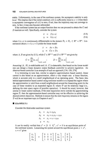
![SMALL-SIGNAL LINEARIZATION 183
Suppose the control objective is to achieve regulation of y with the closed-loop poles
located at s = -1ij and s = -2. Hence the desired characteristic equation is
s3+4s' +6s +4 = 0.
This can be achieved by selecting the control law as
U = -521 - 6 x 2 - 4x3
If the same linear control law is applied to the nonlinear system then we obtain the
following closed-loop nonlinear dynamics:
k 1 = ~ 2 + ~ 2 2 3 (5.7)
x 2 = 2 3 +2 1 2 3 +5 2 1 2 2 +62; +4 2 2 2 3 (5.8)
X3 = - 4 2 1 - 6 x 2 - 4 2 3 - 5 2 1 2 3 - 6 2 2 x 3 - 42;. (5.9)
Linearization of the above closed-loop system (5.7)-(5.9) yields
0 1
X = A + B K = [ 0 0 y ] .
-4 -6 -4
As expected, the eigenvalues of are = -1 ij and X3 = -2. n
5.1.2 Linearizing Around a Trajectory
Consider the nonlinear system system (5.1), where in this case the control objective is to
design a control law such that the state a(t)tracks a desired vector signal zd(t). Let the
tracking error be denoted by e ( t ) = z(t)-ad(t).If a tracking controller is designed based
on a linearization valid at some operating point 2 , E P,
then as ~ ( t )
moves away fromthe
equilibrium point, the state z(t)will try to follow it. However, as the distance between s(t)
and 2, increases, the linear approximation may become increasingly inaccurate. As the
accuracy of the linear approximation decreases, the designed linear controller may become
unsuitable, thus possibly forcing z(t)even further away from the equilibrium 2,.
The tracking objective is in general more suitably addressed by a control law that is
designed based on linearization about the desired trajectory ad(t).Obviously, linearization
around xd(t)assumes that this signal is available apriori. If xd(t)is not available but needs
to be generated online possibly by an outer-loop controller, then small-signal linearization
can be performed around a nominal trajectory z*(t),
which is available apriori. Associated
with a nominal trajectory z*(t) is a nominal control signal u*(t)and initial conditions
z
'
(
0
) = x
: such that z*(t)
satisfies
k*(t)= f(z*(t),u*(t)), 2*(0)= 2;.
Let Z ( t ) = ~ ( t )
- z*(t)and G ( t ) = u(t)- u*(t).
Then
P = f(2,u)- f ( Z * , U * )
= f(5+2*,iL +u*)- f(z*,u*). (5.10)](https://image.slidesharecdn.com/adaptive-approximation-based-controlcompress-230219164415-f6eb4a64/85/adaptive-approximation-based-control_compress-pdf-201-320.jpg)
![184 NONLINEARCONTROLARCHITECTURES
Using the Taylor series expansion off(? + G +u*)around (x*,
v*)we obtain
f ( Z + X * , ii+u*)= f ( X * , U ' ) + .i(z*,u*)j.+ -((2",u*)G+F(t,?,ii)
8.f
dX dU
where F represents the higher-order terms of the Taylor series expansion. Since F contains
the higher-order terms, it satisfies
In other words, as 2 and G become small, 3 goes to zero faster than I/(2,G)11. Using the
Taylor series expansion, (5.10) can be rewritten
In a linear approximation the higher-order terms are ignored. Hence, the small-signal
linearization of (5.1) around the nominal trajectory z*
(t)is given by
i = A(t)z+B(t)G1
where z is the state of the linear model and the matrices A(t) : [0, 03) c) En'" and
B(t): [0, 03) ++PX"
are given by
(5.1 1)
. (5.12)
& Z * , U * ) . . ' &c*,u*)
% ( Z * , U * ) ". g$(z*,u*)
% ( Z * , U * ) ". - q X * , U * )
8%
% ( Z * , U * ) ' ' . &(z*,u*)
x = x * , u=u-
x = x * , u=u-
Now, suppose we select the control law as U. = K(t)z(t).The closed-loop dynamics
for the linear system system are given by
i = [A@)
+B(t)K(t)]
z(t). (5.13)
If the pair (A(t),B(t))is uniformly completely controllable, then there exists K(t)such
that the closed-loop system (5.13) is asymptotically stable; therefore, z(t) -+ 0, which
implies that z(t)+ x*(t).Ifthe nominal trajectory z*(t)
coincides with the desired vector
signal z d ( t ) , then we achieve asymptotic convergence of the tracking error to zero.
Clearly, the above stability arguments were based on the linear model. Applying the
same control law to the nonlinear system we have
4 t ) = K ( t )( 4 t )- Z d ( t ) ) +U * ( t ) ,
which implies
Again, linearizing the closed-loop system around z = X* = z d , u = U* yields
i(t) = f ( X ( t ) , K(t)(x(t)
- X d ( t ) ) +u*(t)).
6(t)= (A(t)+B(t)K(t))
e(t).](https://image.slidesharecdn.com/adaptive-approximation-based-controlcompress-230219164415-f6eb4a64/85/adaptive-approximation-based-control_compress-pdf-202-320.jpg)
![SMALL-SIGNAL LINEARIZATION 185
Therefore, applying the linear control law to the nonlinear system yields a locally asymp-
totically stable closed-loop system. In this case, locality is defined relative to the nominal
trajectory (i.e., /Iz(t)
- x*(t)l/sufficiently small for all t > 0).
If the nonlinear system has an output function then, again, we can proceed to obtain
the C(t)and D(t) matrices. Linearization of the nonlinear system (5.5)-(5.6) around a
nominal trajectory x*(t)produces a linear model of the form
i = A(t)z+B(t)C
= C(t)Z+D(t)C;
where A@),
B(t)are given by (5.11)-(5.12), while C(t)E Wxnand D(t) E W x m
are
given by
x=s.(t), u = u * ( t ) '
Therefore, we see that linearizing around a trajectory yields similar results as linearizing
around an equilibrium point, with the key difference that in the former case the linear model
is time-varying.
Next we present an example of linearizing around a nominal trajectory to illustrate the
concepts introduced in this subsection.
EXAMPLE5.2
A simple model of a satellite of unit mass moving in a plane can be described by the
following equations of motion in polar coordinates [225]:
F(t) = r(t)P(t)- -
P +U
l
(
t
)
r2(t)
where, as shown in Figure 5.2, r(t)is the radius from the origin to the mass, B(t)
is the angle from a reference axis, ul(t) is the thrust force applied in the radial
direction, u2(t)isthe thrust force applied inthe tangential direction, and P is a constant
parameter. With zero thrust forces (i.e., ul(t)= 0 and ug(t) = 0), the resulting
solution can take various forms (ellipses, parabolas, or hyperbolas) depending on
the initial conditions. In this example, we consider a simple circular trajectory with
constant angular velocity (i,e.,r(t)and B ( t ) are both constant). It is easy to verify that
with zero thrusts forces and the initial conditions r(0) = TO, +(O) = 0, O(0) = 00,
b(0) = wo := the resulting nominal trajectory is r*(t)= v0 and B*(t) =
wot +Qo. The objective is to linearize the model around this nominal trajectory.
To construct the state,equation representation, let x
l
(
t
) = r(t),x2(t) = +(t),
x3(t)= B(t),x4(t) = B(t). The equations of motion in the state coordinates are
given by](https://image.slidesharecdn.com/adaptive-approximation-based-controlcompress-230219164415-f6eb4a64/85/adaptive-approximation-based-control_compress-pdf-203-320.jpg)
![SMALL-SIGNAL LINEARIZATION 187
Figure 5.3: Diagram to illustrate the gain scheduling approach, which is based on the
linearization aroundmultiple operating points ( 2 1 , 2 2 , ... 29). The multiple linear models
constitute an example of approximating a nonlinear system.
Consider again the nonlinear system (5.1), where in this case we linearize the system
into N linear models
i = AEz+B,u, i = l , 2, . . . N
where z = z - 2, for each i. Each linear model parameterized by (A,, BE)
is valid
around an operating point point z,. This is illustrated in Figure 5.3, where the nonlinear
function f(z)is linearized around nine operating points {qlzz, .. . zg}. For each linear
model we design a control law based on the control objective associated with a particular
operating point. Suppose that the control law u = K,z corresponds to the linear model
i = A,z +B,u.
A key element of the gain scheduling approach is the design of a scheduler
for switching between the various control lawsparameterized by (K1,
Kz,
.. . K N } .Typ-
ically, transitions between different operating points are handled by interpolation methods.
The gain scheduler can be viewed as a look-uptable with the appropriate logic for selecting
a suitable controller gain K, based on identifying the corresponding operating point 2 , .
Intuitively, we note that if the region of attraction associated with each linearization is
larger than the scheduled operating region corresponding to each operating point, then the
resulting gain scheduling control scheme will be stable. However, special care needs to be
taken since the resulting controller is time-varying, hence the stability analysis needs to be
treated as a time-varying system. A formal stability analysis for gain scheduling is beyond
the scope of this text (see the work of Shamma and Athans [242,243]).
Despite the derivation o f some stability results under certain conditions, gain scheduling
is still considered to some degree an ad hoc control method. However, it has been used in
several application examples, especially in flight control [118, 161, 183, 256, 257, 2581.
The gain scheduling approach has also been utilized in other applications such as in process
control and automotive applications [11, 113, 1261.
One of the key limitations of gain scheduling is that the controller parameters are pre-
computed offline for each operating condition. Hence, during operation the controller is
fixed, even though the linear control gains are changing as the operating conditions change.
In the presence of modeling errors or changes in the system dynamics, the gain schedul-
ing controller may result in deterioration of the performance since the method does not
provide any learning capability to correct-during operation-any inaccurate schedules.
Another possible drawback of the gain scheduling approach is that it requires considerable
offline effort to derive a reliable gain schedule for each possible situation that the plant will
encounter.](https://image.slidesharecdn.com/adaptive-approximation-based-controlcompress-230219164415-f6eb4a64/85/adaptive-approximation-based-control_compress-pdf-205-320.jpg)
![190 NONLINEAR CONTROL ARCHITECTURES
The linearization achieved by the feedback operator (5.15) requires exact knowledge
These comments also apply to feedback linearization when it is applied to higher order
systems.
off and g.The effect of model errors requires further analysis.
Appended Integrators. One role of integrators in control laws is to force the tracking
error to zero in the presence of model error, disturbances, and input type. The required
number of integrators as a function of the type of the input to be tracked is discussed in
most text books on control system design, e.g., [66, 86, 1401. Integrators can have similar
utility in nonlinear control applications. Integrators can be included in the control law and
control design analysis by various approaches such as that discussed in Exercise 1.3 and
the following.
In addition to the tracking error e(t)= y(t) - yd(t) define
(5.17)
where c > 0. It is noted that e F ( t ) is a linear combination of the tracking error and the
integral ofthe tracking error that can be thought of as providing a PI controller (proportional-
integral control). For implementationand analysis, the system state spacemodel will include
one appended controller state to compute the integral of the tracking error. From (5.17),
we obtain e~ = 6 +ce; hence, to force e F ( t ) to zero, the control law (5.15) is modified to
(5.18)
(see also (6.35)). This control law results in 6~ = -ameF. It is easy to see that if e F ( t )
converges to zero then so does e(t) (notice that e = -&
[ e ~ ] ) .
5.2.2 Higher-Order Input-State Linearization
Similar ideas can be developed for n-th order systems in the so called companion form:
> (5.19)
The nonlinearities can be cancelled by using a feedback linearizing control law of the form
1
u = -[-f(x)+v]
g(x)
This results in a simple linear relation (n integrators in series) between v and x,given by
x, = V .](https://image.slidesharecdn.com/adaptive-approximation-based-controlcompress-230219164415-f6eb4a64/85/adaptive-approximation-based-control_compress-pdf-208-320.jpg)
![FEEDBACK LINEARIZATION 191
Therefore, we can choose u as
where e(t) = zl(t)- yd(t) is the tracking error. In this case, the characteristic equation
for the tracking error dynamics of the closed-loop system is
Choosing the design coefficients {Ao, XI, . . . A,-,} so that this characteristic equation
is a Hunvitz polynomial (i.e., the roots of the polynomial are all in the left-half complex
plane) implies that the closed-loop system is exponentially stable and e(t)converges to zero
exponentially fast, with a rate that depends on the choice of the design coefficients.
A important question is: Can all functions in nonlinear systems be cancelled by such
feedback methods?
Clearly, the extent of the designer's ability to cancel nonlinearities depends on the struc-
tural and physical limitations that are applicable. For example, if control actuators could
be placed to allow control of every state independently (an unrealistic assumption in almost
all practical applications), then under some conditions on the invertibility of the actuator
gain g(x),we would be able to use each control signal to cancel the nonlinearities of the
corresponding state. In general, however, it is not possible to cancel all nonlinearities by
feedback linearization methods. To achieve such nonlinearity cancellation, certain struc-
tural properties in the nonlinear system must be satisfied.
A first cut at the class of feedback linearizable systems is nonlinear systems described
by
X = AX +BP-'(z) [U - a(.)], (5.20)
where u is a m-dimensional control input, x is an n-dimensional state vector, A is an n x n
matrix, B is an n x m matrix, and the pair (A,B ) is controllable. The nonlinearities are
contained in the functions cr : 22, H Rm and p : 8, H gZmxm, which are defined on an
appropriate domain of interest, with the matrix p(x) assumed to be nonsingular for every z
in the domain of interest and the symbol P-l denotes an inverse matrix. Systems described
by (5.20) can be linearized by using a state feedback of the form
u = a(.) +P(.).,
which results in
x = Ax +BW
For stabilization, a state feedback w = K z can be designed such that the closed-loop system
x = ( A+ B K ) z is asymptotically stable. This is achieved by selecting K such that all
the eigenvalues of A +BK are in the left-half complex plane. A similar design procedure,
based on linear control designed methods, can be used to select w for tracking problems.
The reader will undoubtedly notice that the class of systems described by (5.20) is
significantly more general than the class of nonlinear systems in companion form (5.19).
The class of feedback linearizable systems is actually even larger than the systems described
by (5.20) since it includes nonlinear systems that can be transformed to (5.20) by a coordinate
transformation. This topic is discussed in detail in the next subsection.
If a nonlinear system is not feedback linearizable, it does not imply that it cannot be
controlled. Thereareseveral classes ofnonlinear systems that cannotbe put into the standard
form for feedback linearizable systems, but they can be controlled by other methods.](https://image.slidesharecdn.com/adaptive-approximation-based-controlcompress-230219164415-f6eb4a64/85/adaptive-approximation-based-control_compress-pdf-209-320.jpg)
![194 NONLINEAR CONTROLARCHITECTURES
Once a diffeomorphism T ( z )is defined then it is possible to follow a similar procedure
as for linear systems to derive the model appropriate relative to the new set of coordinates
z = T(z).Consider the following affine nonlinear dynamical system:
(5.23)
where j z : R, H En,G
, : R, H PX"
and h, : R, H R P are smooth functions in a
region R, c P.The above system can be transformed to a new state coordinate system
z = T ( z ) ,
where T is a diffeomorphism. In the new z-coordinate, the system is described
bv
(5.24)
where
It is important to note that, while in linear change of coordinates the transformation is
always global (i.e., T it is a global diffeomorphism), for nonlinear change of coordinates it
is often the case that the transformation is local.
Following the development of the concept of a diffeomorphism, we can now define the
class of feedback linearizable systems. A nonlinear system
j
.= f(s)
+G(s)u (5.25)
is said to be input-statefeedback linearizable if there exists a diffeomorphism z = T(z),
with T(0)= 0, such that
i = AZ+B ~ - ' ( z )
[U - ~ ( z ) ] , (5.26)
where (A, B ) is a controllable pair and p(z) is an invertible matrix for all z in a domain
of interest D, c P.
Therefore, we see that the class of feedback linearizable systems includes not only
systems described by (5.20), but also systems that can be transformed into that form by
a nonlinear state transformation. Determining if a given nonlinear system is feedback
linearizable and what is an appropriate diffeomorphism are not obvious issues, and in
fact they can be extremely difficult since in general they involve solving a set of partial
differential equations.
Given a nonlinear system (5.25), consider a diffeomorphism z = T(s). In the z-
coordinates we have
dT dT
d X dX
i. = -
f
(
.
) +-G(z)u.
For feedback linearizable systems, (5.27) needs to be of the form
i = Az +BP-'(z) [u
- a(.)]
= AT(x)- BP-'(T(Z))Q(T(Z))
+BP-l(T(z))u.
(5.27)](https://image.slidesharecdn.com/adaptive-approximation-based-controlcompress-230219164415-f6eb4a64/85/adaptive-approximation-based-control_compress-pdf-212-320.jpg)
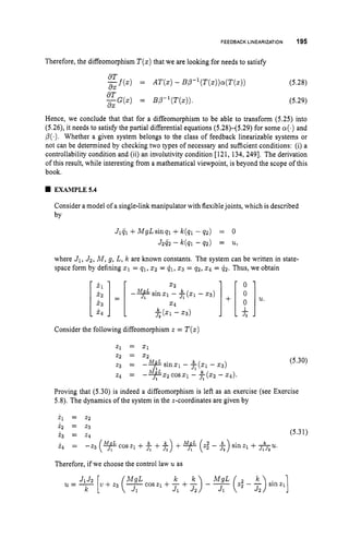
![FEEDBACK LINEARIZATION 199
and the r-th derivative of y ( t ) satisfies
y(') = CA'x +CAT-' Bu.
Moreover, the dynamics of the linear system can be broken up into two components as
follows:
4 = Pv+QC (5.41)
( = AoC +Bo [C(" +C,Tq +ku] (5.42)
Y = c
o
c (5.43)
where q E IfZ"-', c E %', the triple (Ao, Bo, CO)is a canonical form representation of r
integrators, as described by (5.39), P and Q are matrices of appropriate dimension, C
c is
a vector of dimension r, and C, is a vector of dimension (n- r).
The reader will note that (5.41)-(5.43) is a linear special case of the normal form de-
scribed by (5.36H5.38). The zero dynamics of the linear system, as defined earlier for the
general normal form of nonlinear systems, are obtained by setting C = 0 in (5.41). This
yields
7j = Pq. (5.44)
The stability of the zero dynamics are determined by the eigenvalues of P. The model is
said to be minimum phase if all the eigenvalues are in the left open-half complex plane. It
is important to note that the eigenvalues of P turn out to be the same as the roots of the
numerator of the transfer hnction H(s). This justifies the use of the term zero dynamics
for nonlinear systems.
One question that may be raised in obtaining the normal form for nonlinear systems is
whether any system can be put into the canonical normal form. In general, the answer is
negative since for some systems the relative degree is undefined. This may happen, for
example, if L,Lqh(z) = /coal, where ko is a scalar constant. This implies that L,L$h(z)
is zero for z1= 0 but it is nonzero in any neighborhood of z1 = 0.
Next, we consider the tracking control design for input-output feedback linearizable
systems. We assume that the control objective is for y ( t ) to track a desired signal yd(t).
Let e(t) = y(t) -yd(t)be the tracking error. Starting from the normal form (5.36)-(5.38)
we design the feedback control law
u = 0 0 ( ? 7 , e ) +Po(77, O V
where v is selected as follows:
(5.45)
(5.46)](https://image.slidesharecdn.com/adaptive-approximation-based-controlcompress-230219164415-f6eb4a64/85/adaptive-approximation-based-control_compress-pdf-217-320.jpg)
![200 NONLINEAR CONTROLARCHITECTURES
Therefore, by appropriately selecting the coefficients {ko, k1, ... k,-2, kT-l} the roots
of the characteristic equation
sr +k,-lST-l +k r - 2 S T 4 + .’ . +k1s +ko = 0
can be arbitrarily assigned. This implies that the tracking error can be made to converge to
zero asymptotically (exponentially fast).
From the normal form (5.36)-(5.38), we note that the above control design has taken care
only of the ( variables. The designer also needs to be assured that the internal dynamics,
+ = $(7,(), remain bounded when the control law is designed for the (-dynamics. This
issue is addressed next.
Let
T
g d ( t ) = [l/d(t) Y d ( t ) l/r’(t) ’ ‘ ’ Y!-”(t)]
As shown by Isidori [1211,ifwe assume that g d ( t ) is bounded for all t 2 0 and the solution
of
is well defined, bounded, and uniformly asymptotically stable, then using the control law
(5.45)-(5.46) guarantees that the whole state remains bounded and the tracking error e(t)
converges to zero exponentially fast.
In the special case of regulation to the origin; i.e., yd(t) = 0 for all t 2 0, then it is
required that the zero dynamics
are asymptotically stable in order to ensure that the overall system states remain bounded
and the tracking error converges to zero.
In summary, we note that for input-output linearizable systems there are two components
to be taken care of:
the (-dynamics, which can be linearized by the control variable u,
and
the 7-dynamics, referred to as internal dynamics, which are rendered unobservable
by the u defined in (5.33, but which need to have some stability properties (minimum
phase) in order to allow stable control of the overall system.
$ = d’(7,g d ( t ) ) , 7(0)= 0
4 = d47,O)
EXAMPLE~S
Consider the flexible manipulator model of Example 5.4,
whose state representation
is given by
First consider the case where the output y = 2 1 . In this case the diffeomorphism
2 = T ( s )given by (5.30) transforms the system into the normal form since
(5.47)](https://image.slidesharecdn.com/adaptive-approximation-based-controlcompress-230219164415-f6eb4a64/85/adaptive-approximation-based-control_compress-pdf-218-320.jpg)
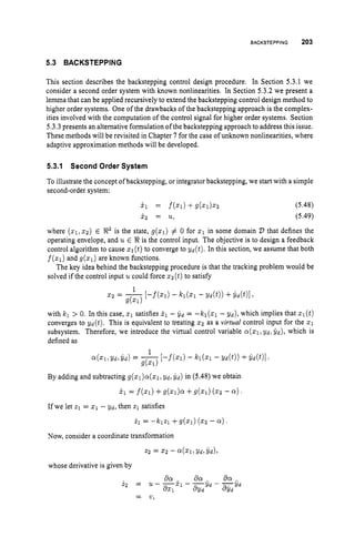
![BACKSTEPPING 205
A key assumption in the above backstepping procedure is that both f(q)
and g(z1)
are known exactly. In the case where they are partially or completely unknown then
it may be appropriate that these functions be estimated online, which is the topic of
discussion in the next two chapters.
5.3.2 Higher Order Systems
Consider the system model
j.1 = fl(Z1) +91(21)22 (5.55)
j.2 = f2(z)+gz(z)U. (5.56)
where z = [z: ~ $ 1 ’ E Snand x2 E S1.Define %1 = z1 - Y d where Yd(t) is the
signal vector to be tracked. For this system, we assume that we know scalar virtual control
functions a ( z 1 , Ydr&) and positive definite V1(zl) such that
av1
a21
(5.57)
-[fl+g l a - Gd] 5 -Wl(zl)
where Wl(zl) is a positive definite function. Our objective is to define u such that the
system of equations (5.55)-(5.56) will have 2
1 tracking Y d (ix., 21 convergent to zero).
We define 22 = 2 2 - a.Then the ( ~ 1 ~ 2 2 )
dynamics are described by
21 = fl(z1) +gl(z1)a +91(21)%2- G d (5.58)
i 2 = f2(z)+g2(z)u -ix (5.59)
where
Consider V(zl,t2) = VI(z1) + $ 2 ; . The time derivative of V along the solutions of
(5.58)-(5.59) is given by
av1
3%
1
I -
W
1
(
Z
1
)
+ -g1(z1)22 +22 (fd. ) +92(z 1
. -
Therefore, if g2(z) # 0 and the control signal 2~ is selected as
(5.60)
with IC2 > 0 being a design parameter, then we have
v 5 -W1(21) - IC2.t;
which is negative definite.
Therefore, we have proven Lemma 5.3.1.Note that this lemma can be applied recursively
to achieve tracking control for higher order systems.
Lemma 5.3.1 Givenasystem intheform oS(5.55)-(5.56)andknown functionsal(z1, yd, yd)
andpositive dejnite Vl(zl) satisfying (5.57), thenfor u specijied according to (5.60), the
tracking error dynamics of (5.58)-(5.59) are asymptotically stable. IfV
1 is radially un-
bounded and all assumptions hold globally, then the tracking error dynamics are globally
asymptotically stable.](https://image.slidesharecdn.com/adaptive-approximation-based-controlcompress-230219164415-f6eb4a64/85/adaptive-approximation-based-control_compress-pdf-223-320.jpg)
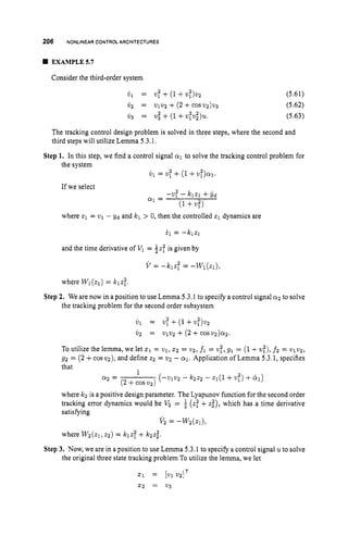
![BACKSTEPPING 207
0
g1 = [ 2+c0sv2 ]
f 2 = v3”
gz = (l+V:v,”)
and define z3 = v3 - 0 2 . Application of Lemma 5.3.1, specifies that
(-Vi -
1
21=
(1+v;v,’,
where k3 is a positive design parameter. As a result of the lemma, the control law
given by (5.64) results in globally exponentially stable tracking error dynamics.
Implementation ofthiscontroller requires analytic computation ofal, C
Y
l
, 012, CYz, and
finally u.These computations will involve Y d , Gd, and i d . In general, the computation
of the quantities CY, can be algebraically tedious, especially for systems of order larger
than two or three. a
5.3.3 Command Filtering Formulation
Much of the complexity that arises in the backstepping control laws that result from recursive
application of Lemma 5.3.1 is due to the computation of the time derivative of the virtual
control variables ai(xlr...,xi,Y d , ...,yy)). The computation of these time derivatives
becomes even more complex in applications where the functions f and g are approximated
online. This section presents an alternative formulation of the backstepping approach that
decreases the algebraic complexity ofthe backstepping control law from that ofeqn. (5.54).
Consider the second-order system
(5.65)
(5.66)
where z = [z1x2IT E Rzis the state, 5 2 E !R1, and u is the scalar control signal. A
region D is the specified operation region of the system. The functions fi, gi for i = 1 , 2
are known locally Lipschitz functions. The functions gi are assumed to be nonzero for all
z E D.There is a desired trajectory zlc(t),with derivative &(t), both of which lie in a
region D fort 2 0 and both signals are assumed known. Define the tracking errors
51 = 2 1 - X I c
52 = 2 2 - X z c
where xzc will be defined by the backstepping controller. Let
(5.67)
al(z1,51,
X l C ) = - [-fl - k151 +kl,] with kl > 0
be a smooth feedback control and define the smooth positive definite function Vl(5.1) =
?z x such that
1
91
1 - T -
~av1 [fl+QlQl- &I = -W@d (5.68)
851](https://image.slidesharecdn.com/adaptive-approximation-based-controlcompress-230219164415-f6eb4a64/85/adaptive-approximation-based-control_compress-pdf-225-320.jpg)
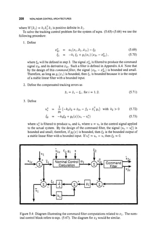
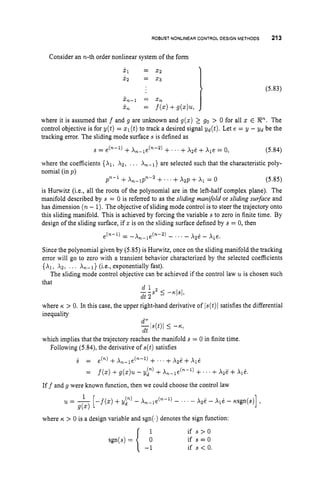
![216 NONLINEARCONTROL ARCHITECTURES
Moreover, we assume that the uncertainty satisfies a so-called matching condition:
(5.90)
(5.91)
The matching condition implies that the uncertainty terms appear in the same equations as
the control inputs u,
and as a result they can be handled by the controller.
By substituting (5.88)-(5.89) and (5.90)-(5.91) in (5.87) we obtain
= fo(z)+G
o
(
.
) (u+d z ,u)),
where 17 comprises all the uncertainty terms, and is given by
~ ( z ,
u)= A; +A&u.
(5.92)
The Lyapunov redesign method addresses the following problem: suppose that the equi-
librium of the nominal model x = fo(z)+Go(z)ucan be made uniformly asymptotically
stable by using a feedback control law u = PO(%). The objective is to design a corrective
control function p*(z)such that the augmented control law u = po(z)+p*(z)is able to
stabilize the system (5.92) subject to the uncertainty ~ ( z !
u)being bounded by a known
function.
Next, we consider the details of the Lyapunov redesign method, which is thoroughly
presented for a more general case in [134]. We assume that there exists a control law
u = po(z) such that z = 0 is a uniformly asymptotically stable equilibrium point of the
closed-loop nominal system
We also assume that we know a Lyapunov function Vo(z)that satisfies
(5.94)
where 01, 0 2 , 0 3 : %+ +-+ 92’ are strictly increasing functions that satisfy ~ ~ ( 0 )
= 0 and
a i ( ~ )
-+ 03 as r -+ m. These type of functions are sometimes called class Ic, functions
[134].
The uncertainty term is assumed to satisfy the bound
tlv(z1u)llm I
ij(t>.) (5.95)
where the bounding function ij isassumed to be known apriori or available formeasurement.
Now, we will proceed to the design of the “corrective control” component pi (z) such that
u = po +p‘ stabilizes the class of systems described by (5.92) and satisfying (5.95). The
corrective control term is designed based on a technique following the nominal Lyapunov
function VO,
which justifies the name Lyapunov redesign method.
Consider the same Lyapunov function VO
that guarantees the asymptotic stability of the
nominal closed-loop system, but now consider the time derivative of V
o along the solutions
of the full system (5.92). We have](https://image.slidesharecdn.com/adaptive-approximation-based-controlcompress-230219164415-f6eb4a64/85/adaptive-approximation-based-control_compress-pdf-234-320.jpg)
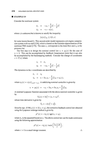
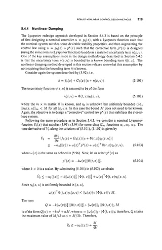
![220 NONLINEARCONTROLARCHITECTURES
Since ~ ~ ( 1 1 ~ 1 1 )
is strictly increasing and approaches 03 as (/z11+ co,there exists a ball
B, of radius p such that VOI 0 for z outside 0,.Therefore, the closed-loop system is
uniformly bounded and the trajectory z(t)converges to the invariant set
where p can be made smaller by increasing the feedback gain k or by decreasing the infinity
norm of the model error.
EXAMPLE 5.10
Consider the nonlinear model of Example 5.9. In this case, instead of assuming that
l/qz(z)//
I
:fje(z)where fjz(z)is known, we assume that qz(z)= @(z)qo(z) where
0 is known, while qo is unknown but uniformly bounded.
The corrective control term obtained using the nonlinear damping method is given
by
P " ( S ) = - 2 k h +dll@(kz)ll;.
redesign method. n
It is noted that this control law is not switching as it was in the case of the Lyapunov
5.4.5 Adaptive Bounding Control
Of the four techniques presented in this section, namely bounding control, sliding mode
control, Lyapunov redesign, and nonlinear damping, the first three are based on the key
assumption of a known bound on the uncertainty. The nonlinear damping technique does
not make this bounding assumption; however, the resulting stability property does not
guarantee the convergence of the tracking error to zero, but to an invariant set whose radius
is proportional to the m-norm of the uncertainty. Even though the residual error in the
nonlinear damping design can be reduced by increasing the feedback gain parameter k ,
this is not without drawbacks, since increasing the feedback gain may result in high-gain
feedback ,with all the undesirable consequences.
In this subsection, we introduce another technique which also relaxes the assumption of
a known bound. Specifically, it is assumed that q(z.u ) is bounded by
where 0 is an unknown parameter vector of dimension q and p is a known vector function.
Since B T p represents a bound on the uncertainty, each element of 8 and p is assumed to
be non-negative. Typically, the dimension q is simply equal to one. However, the general
case where both 8 and p are vectors, allows the control designer to take advantage of any
knowledge where the bound changes for different regions of the state-space z. If a known
function p(z) is not available, it can be simply assumed that /lv(zr
Z L ) / ~ ~
5 8, where 8 is a
scalar unknown bounding constant. The adaptive bounding control method was introduced
in [215] and was later used in neural control [209].
It is worth noting that the bounding assumption ofthe adaptive bounding control method
is significantly less restrictive than that of the Lyapunov redesign method where the bound
is assumed to be known. Even though one may consider simply increasing the bound of the
Lyapunov redesign method until the assumed bound holds, this is not always possible, and](https://image.slidesharecdn.com/adaptive-approximation-based-controlcompress-230219164415-f6eb4a64/85/adaptive-approximation-based-control_compress-pdf-238-320.jpg)
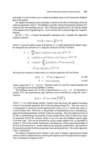
![222 NONLINEAR CONTROL ARCHITECTURES
5.5 ADAPTIVE NONLINEARCONTROL
Adaptive control deals with systems where some of the parameters are unknown or slowly
time-varying. The basic idea behind adaptive control is to estimatethe unknown parameters
online using parameter estimation methods (such as those presented in Chapter4), and then
to use the estimated parameters, in place of the unknown ones, in the feedback control law.
Most of the research in adaptive control has been developed for linear models, even though
in the last decade or so there has been a lot of activity on adaptive nonlinear control as well.
Even in the case of adaptive control applied to linear systems, the resulting control law is
nonlinear. This is due to the parameter update laws, which render the feedback controller
nonlinear.
There are two strategies for combining the control law and the parameter estimation
algorithm. In the first strategy, referred to as indirect adaptive control, the parameter
estimation algorithm is used to estimate the unknown parameters of the plant. Based on
these parameter estimates, the control law is computed by treating the estimates as if they
were the true parameters, based on the certainty equivalence principle [111. In the second
strategy, referred to as direct adaptive control, the parameter estimator is used to estimate
directly the unknown controller parameters.
It is interesting to note the similarities and difference between so called robust control
laws and adaptive control laws. Therobust approaches, which were discussedin Section5.4,
treat the uncertainty as an unknown box where the only information available are some
bounds. The robust control law is obtained based on these bounds, and in fact is designed
to stabilizes the system for any uncertainty within the assumed bounds. As a result, the
robust control law tends to be conservative and it may lead to large control input signals
or control saturation. On the other hand, adaptive control assumes a special structure for
the uncertainty where the nonlinearities are known but the parameters are unknown. In
contrast to robust control, in adaptive control the objective is to try to estimate the uncertain
(or time-varying) parameters to reduce the level of uncertainty.
In the next chapter, we will start investigating the adaptive approximation control ap-
proach where the uncertainty also includes nonlinearities that are estimated online. Hence,
adaptive approximation based control can be viewed as an expansion of the adaptive con-
trol methodology where instead of having simply unknown parameters we have unknown
nonlinearities.
Adaptive control is a well-established methodology in the design of feedback control
systems. The first practical attempts to design adaptive feedback control systems go back
as far as the 1950s, in connection with the design of autopilots [295]. Stability analysis
of adaptive control for linear systems started in the mid-1960s [196] and culminated in
1980with the complete stability proof for linear systems [69, 177, 1801. The first stability
results assumed that the only uncertainty in the system was due to unknown parameters;
i.e., no disturbances, measurement noise, nor any other form of uncertainty. In the 1980s,
adaptive control research focused on robust adaptive control for linear systems, which dealt
with modifications to the adaptive algorithms and the control law in order to address some
types of uncertainties [1191. In the 1990s, most of the effort in adaptive control focused on
adaptive control of nonlinear systems with some elegant results [1391.
To illustrate the use of the adaptivecontrol methodology we consider below twoexamples
of adaptive nonlinear control.](https://image.slidesharecdn.com/adaptive-approximation-based-controlcompress-230219164415-f6eb4a64/85/adaptive-approximation-based-control_compress-pdf-240-320.jpg)
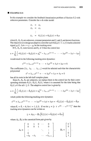
![EXERCISES AND DESIGNPROBLEMS 227
5. Design a feedback controller u = klzl +lc2z2 such that the poles of the closed-loop
system for the linear model are located at s = -1 fj .
Exercise 5.3 Use a simulation study to investigate the performance of the linear feedback
control law
developed in Exercise 5.2 when applied to the original nonlinear system. Consider several
initial conditions close to the equilibrium point 5 = z* to get a rough idea of how large is
the region of attraction around the equilibrium point.
Exercise 5.4 Use a simulation study for the satellite example of Example 5.2. Assume
that: p = 10; q ( 0 ) = TO = 10; z2(0) = +(O) = 0;q ( O ) = 80 = 0. Consider the
following cases:
(a) ~ ( 0 )
= 0.1, ul(t) = 0, u2(t)= 0;
u = ICl(51 - 1)+kz(52 - 1)
(b) 54(0) = 0.095, ul(t) = 0, u2(t)= 0;
(c) 5 4 ( 0 ) = 0.105, ul(t) = 0, uz(t)= 0;
(d) 54(0) = 0.1, ul(t)= 0.02, u2(t)= 0;
(e) z4(0)= 0.1, ul(t) = 0.1sin(t), uz(t)= 0.1cos(t);
(f) x4(0) = 0.09, W(t) = 0, uz(t)= O.lcos(t).
Simulate the differential equation for about 100 s. Provide plots of the satellite motion
in Cartesian coordinates instead of polar coordinates. Interpret your results. Compare the
solution of the nonlinear differential equation with that of the linearized model (assume
that TO = 10; 80 = 0; w = 0.1). Discuss the accuracy of the linearized model as an
approximation of the nonlinear system. Plot the trajectories of the satellite motion of both
the linear and nonlinear model on the same diagram for comparison purposes.
Exercise 5.5 Consider the nonlinear state equation
u(t)
51(t)u(t)
- 5 3 ( 9
5 2 (t)- 253 (t)
Y(t) = z 2 ( t ) - 2%3(t)
[z] = [
with the nominal initial state zI(0) = 0, xZ(0) = -3, z
: (0) = -2, and the nominal input
u*(t)= 1. Show that the nominal output is y*(t) = 1. Linearize the state equation about
the nominal solution.
Exercise 5.6 Consider the following second-order model which represents a field con-
trolled DC motor [2481
i 1 = -50x1 - 0 . 4 5 2 U +40
X 2 = -5X2 + ~ O O O O X ~ U
y = 5 2
where 51 is the armature current, 5 2 is the speed, and uis the field current. It is required to
design a speed control system so that y(t) asymptotically tracks a constant reference speed](https://image.slidesharecdn.com/adaptive-approximation-based-controlcompress-230219164415-f6eb4a64/85/adaptive-approximation-based-control_compress-pdf-245-320.jpg)


![PERSPECTIVEFOR AOAPTIVEAPPROXIMATION
BASED CONTROL 235
If the derived nominal control law
u = ko(z)+B,(z)K,T(z)
is applied to the full model of eqn. (6.l), then the closed-loop dynamics will be
different. Specifically, ifwe let f*(z)
= f(z)
- fo(z)
and G*(z) = G(z) - G,(z)
then we obtain
j. = fo(z)+G,(x)ko(z)+Go(s)B,(~)KzT(z)
+A*(x)
where
In the z-domain, the closed-loop system is given by
A*(z) = f * ( ~ )
t G*(z)ko(z)
+G*(Z)B,(Z)K,T(~)
The motivation for using adaptive approximation can be viewed as. a way to esti-
mate during operation the unknown functions f*(z) and G*(z)by f(z;
Of.8f)
and
G(z;&. 8 ~ ) ,
respectively,and use theseapproximations to improvetheperformance
of the controlled system. If the initial weights ofthe adaptive approximators are cho-
sen such that f(z;
ef(O), ef(0))= 0 and G(s;e G ( o ) , ~ . G ( O ) )= 0 for all z, then at
t = 0the control law is the same as the nominal tontrol law u
,
.During operation, the
objective is for the adaptive approximators f(z;
ef(t),
B f ( t ) )and G(z;e.G(t),8 . ~ ( t ) )
to learn the unknown functions such that they can be used in the feedback control
law. The sought enhancement in performance can be in the form of a larger region
of attraction (Le., loosely speaking, a larger region of attraction implies that initial
conditions further away from the equilibrium still convergeto the equilibrium), faster
convergence, or more robustness in the presence of modeling errors and disturbances.
a
To illustrate some key concepts in adaptive approximation based control, it is useful to
consider the stability properties of the equilibrium of the closed-loop system in terms of the
size of the region of attraction. Let us define the following type of stability results [1341.
For better understanding, the definitions are provided for a scalar system with a single state
y ( t ) . We let the initial condition y(0) be denoted by yo.
0 Local Stability. The results hold only for some initial conditions yo E [-a, b],where
a, b are positive constants, whose magnitude may be arbitrarily small. In addition,
the values of a and b are determined by f’ which is unknown; hence a and b are
unknown.
0 Regional Stability. The results hold only for some initial conditions that belong to a
known and predetermined range yo E [-a, b]. Typically, the magnitude of a and b
is not “too small.”
0 Semi-global Stability. In this case, the stability results are valid for any initial con-
ditions yo E [-a: a],where a is a finite constant that can be arbitrarily large. The
value of a is determined by the designer.
0 Global Stability. The stability results hold for any initial condition yo E 8.](https://image.slidesharecdn.com/adaptive-approximation-based-controlcompress-230219164415-f6eb4a64/85/adaptive-approximation-based-control_compress-pdf-253-320.jpg)
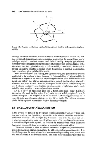
![STABILIZATIONOF A SCALAR SYSTEM 237
section will be expanded to the tracking problem in Section 6.3 and then extended to more
realistic higher order systems in Chapter 7.
Consider the scalar system described by
Y = f b )+% d o ) = Yo (6.4)
where u E R1is the controlled input, y E 8’is the measured output, and f(y) is an
unknown nonlinearity. Without loss of generality we assume that f(0) = 0. To allow the
possibility of incorporating any available information into the control design, we assume
that f is made of two components:
where f,(y) is a known function representing the nominal dynamics of the system, and
f’(y) is an unknown function representing the nonlinear uncertainty. The control objective
is to design a control law (possibly dynamic) such that u(t)and y(t) remain bounded and
y(t) converges to zero (or to a small neighborhood of zero) as t + 00.
The following subsections will lead the reader through a series of different assump-
tions and design techniques that will yield different stability results and will provide some
intuition about the achievable levels of performance and the trade-offs between different
techniques.
6.2.1 Feedback Linearization
First consider the casewhere the nonlinear function f is known (i.e., assume that f *(y) = 0
for all y E 8).In this simple case, we saw in Chapter 5 that the control law
u = -a,y -f(y) = -a,y - f,(y) with a, > 0 (6.5)
achieves the desired control objective since the closed-loop dynamics y = -a,y make the
equilibrium pointy = 0 asymptotically stable. In fact, y(t) converges to zero exponentially
fast.
Obviously, if the function f(y) is known exactly for all y E R1,
the stability results are
global. On the other hand, if f(y) is known only for y E [-a, b]then the stability results
are regional, assuming that we use the same control law as in eqn. (6.5). Specifically, if the
initial condition yo belongs in the range [-a, b],then y(t) converges to zero exponentially
fast; otherwise it may not converge.
The reader will recall from Chapter 5 that this control strategy is known as feedback
linearization. It is based on the simple idea that if all the nonlinearities of the system are
known and of a certain structure suchthat they can be “cancelled” by the controlled variable
u, then the feedback control law is used to make the closed-loop dynamics linear. Once
this is achieved, then standard linear control techniques can be used to achieve the desired
transient and steady-state objectives.
As discussed in Chapter 5, the practical use of feedback linearization techniques faces
some difficulties. First, not all nonlinear systems are feedback linearizable. Second, in
many practical nonlinear systems some of the nonlinearities are “useful” (in the sense
that they have a stabilizing effect) and therefore it is not advisable to employ significant
control effort for cancelling stabilizing components of the system. Thirdly, and perhaps
most importantly, in most practical systems the nonlinearities are not known exactly, or
they may change unpredictably during operation. Therefore, in general, it is not possible to](https://image.slidesharecdn.com/adaptive-approximation-based-controlcompress-230219164415-f6eb4a64/85/adaptive-approximation-based-control_compress-pdf-255-320.jpg)
![238 ADAPTIVE APPROXIMATION:MOTIVATION
AND ISSUES
achieve perfect cancellation of the nonlinearities, which motivates the use of more advanced
control approaches to handle uncertainty. The effect on the closed-loop performance of
inaccurate cancellation of the nonlinearities was illustrated in the simple example discussed
in Chapter I.
6.2.2 Small-SignalLinearization
Next, suppose that we linearize the nonlinear system around the equilibrium point y = 0,
and then employ a linear control law. In this case, the linearized system is given
Therefore, the linear control law u = -(a* +a,)y results in the closed-loop dynamics
Consider the Lyapunov function V = iy2
eqn. (6.6) is
dV 2
-= -
a
,
y +
dt
Thus, the region of convergence is
The time derivative of V along the solutions of
Therefore, the linear control law, applied to the nonlinear system, results in local stability
results. Specifically, ifthe initial condition yo is in A,then we have asymptotic convergence
to zero. According to the fundamental theorem of stability (see Chapter 5), the size of
the region A can be arbitrarily small, depending on the nature of f ( y ) relative to that
of its linearization. In this case, we cannot quantify a specific range [-a, b] without
additional assumptions about the nature o f f . The designer can increase the size of the
set A by increasing a, (i.e., high-gain control); however, this is an undesirable approach
to increasing the domain of attraction, as the parameter a, determines the bandwidth of
the control system. Increasing a, to enlarge the theoretical domain of attraction would
necessitate faster (more expensive actuators) and might result in excitation of previously
unmodeled higher frequency dynamics. The use of high-gain feedback is particularly
problematic in the presence of measurement noise. For special classes ofnonlinear systems,
it may also result in large transient errors, which is known as the peaking phenomenon
[134,263].
EXAMPLE6.2
Consider the scalar example
The linearized system is given by 61 = u, which can be easily controlled by a linear
control law of the form u = -a,yl, a, > 0. If we apply the same linear control
law to the original (nonlinear) system, the resulting closed-loop system is given by
y = -
a
,
y +Icy
jl = Icy2 +u
2](https://image.slidesharecdn.com/adaptive-approximation-based-controlcompress-230219164415-f6eb4a64/85/adaptive-approximation-based-control_compress-pdf-256-320.jpg)
![240 ADAPTIVE APPROXIMATION MOTIVATIONAND ISSUES
I
Figure 6.3: Plot illustrating the smooth approximation of v(y). The upper bound fu(y)
is plotted above the y-axis, while the lower bound f~(y) is plotted below the y-axis. The
function v(y)of eqn. (6.9) is plotted as the bold portion of f~ and fualong with the bold
dashed line for y E [-E; E ] .
satisfies
Therefore, using Lemma A.3.2,given any ,
L
L > 2 there exists a time Tpsuch that for all
t 2 Tpwe have V ( t )5 p. This implies that asymptotically (as t + m),the output y(t)
satisfies Iy(t)i 5 d x .
Therefore, by combining the stability analysis for both regions A
1 and A:!we obtain
that asymptotically the output y ( t ) goes within a bound which is the minimum of E and
d G . We notice that as E becomes smaller, the residual regulation error y ( t ) also
becomes smaller; however, the control switching frequency increases. In the limit, as E
approaches zero, the control law becomes discontinuous and the output y ( t ) converges to
zero asymptotically.
The feedback control law used in this subsection employs the known bounding functions
f~(y), fu(y) toguarantee that the feedback system is ableto handle the worst-case scenario
of the unknown nonlinearity. However, this may result in unnecessarily large control efforts
(high-gain feedback), and also possibly degraded transient behavior. Although the closed-
loop stability, as we saw earlier, can be guaranteed, from a practical perspective there are
some other issues that the designer needs to be aware of:
0 Large control efforts may be undesirable due to the additional cost.
In practice, the control input generated by the controller can be implemented only if it
is within a certain range. High-gain feedback may cause saturation of the controller,
which can degrade the performance or even cause instability.
0 In the presence of noise or disturbances, high-gain feedback may perform poorly
and can result in instability. The robustness issue is quite critical in practice because
measurement noise is inherently present in most feedback systems. Intuitively, we](https://image.slidesharecdn.com/adaptive-approximation-based-controlcompress-230219164415-f6eb4a64/85/adaptive-approximation-based-control_compress-pdf-258-320.jpg)
![STABILIZATIONOFA SCALAR SYSTEM 241
can see that measurement noise will appear to the controller as small tracking errors,
which with a high-gain control scheme can cause large actuation signals that may
result in significant tracking errors.
Typically,the mathematical model on which the control design is based is the result
of a reduced-order simplification of the actual plant. For example, the real plant may
be of order 20,while the model used for control design may be 3rd order. Such model
reduction is achieved by ignoring the so-called fast dynamics. Unfortunately, high-
gain feedback may excite these fast dynamics, possibly degrading the performance
of the closed-loop system.
The extend to which these are critical problems depends on the specific application
and the amount of uncertainty. In some applications the plant is quite susceptible to the
problems of high-gain feedback and switching, while in others there is significant margin
of tolerance. The magnitude of uncertainty also plays a key role. The level of uncertainty
is represented by the difference between f ~ ( y )
and fcr(y). If the difference is ‘‘large’’then
that is an indication that the range in which the uncertainty f* may vary is large, and thus
the control design team would need to be conservative, which results in larger control effort
than necessary. Onthe other hand, ifthebounding functions selected donot hold in practice,
then stability of the closed-loop system cannot be guaranteed. Twomethods to decrease the
conservatism are to approximatethe nonlinearity f’ and to estimate the bounding functions
f ~ ( y )
and fu(y). These methods are considered in the sequel.
6.2.4 Adaptive BoundingMethods
One approach to try to reduce the amount of uncertainty, and thus have a less conservative
control algorithm, is to use adaptive bounding methods [215]. According to this approach,
the unknown function f* is assumed to belong to apartidly known range as follows:
W f i ( Y ) I f*(Y) I Qufu(Y)
where fi and fu are known positive lower and upper bounding functions, respectively,
while a
1 and a, are unknown constant parameters multiplying the bounding functions.
The unknown parameters al, a, can be positive or negative depending on the nature of
the bounding functions fi(y) and f,(y). The procedure that we will follow is based on
estimating online the unknown parameters ai, a, and using the estimated parameters in
the feedback control law. It is noted that the above condition is similar to the sector
nonlinearity condition which has been considered in terms of absolute stability of nonlinear
systems [134].
The advantage of this formulation over a fixed bounding method is that it allows the
design of control algorithms for the case where the bounds are not known. The function
fi (y) (correspondingly fU (y)) represents the general structure of the uncertainty, however
the level of uncertainty is characterized by the unknown parameter a
1 (correspondingly
a,). In the absence of any information about the uncertainty, the bounding functions can
both be taken to be fl(y) = f,(y) = 1.
Now, the control law is given by
(6.10)
(6.11)](https://image.slidesharecdn.com/adaptive-approximation-based-controlcompress-230219164415-f6eb4a64/85/adaptive-approximation-based-control_compress-pdf-259-320.jpg)
![244 ADAPTIVE APPROXIMATION: MOTIVATIONAND ISSUES
By this time the reader can recognize this as a rather standard adaptive scheme with the
time derivative of V satisfying
T
v = -amY2 +y ~ f ( y )
+ (B- e*) r-1 (e - rd(y)y). (6.16)
Therefore, if we select the adaptive update algorithm for e(t)as
e = rd(Y)Y, (6.17)
then the Lyapunov function derivative satisfies
v = -amy2 +yPf(y). (6.18)
Let us try to understand better the effect of Ef(y) on stability. First, assume that the
MFAE satisfies Ef (y) = 0 for all y E V = {/y/ 5 a}. In this case, V = -amy2 for y
in the region lyI 5 a. If ly(t)l > a for some t > 0, then nothing can be said about the
stability of the present feedback system, as the present controller does not address Pf(y)
outside of V.If the initial condition y(0) = yo satisfies (yo15 a there is no guarantee
that ly(t)l 5 a for all t 2 0, since the Lyapunov function V depends on both y and 8.
Whether or not y(t) remains within [-a, a]depends on the initial parameter estimation
error e(0)- 6*, in addition to the initial condition yo. Moreover, the closed-loop stability
properties depend critically on design variables such as the learning rate matrix r and the
selected feedback pole location a
,
.
Thistype ofsituation iscommonlyfound inthe use ofapproximators infeedback systems.
In general, adaptive approximation methods provide reasonably accurate approximation of
the uncertainty over a certain region of the state space denoted by V,
while not providing
accurate approximation in the rest of the state space (outside the approximation region).
Therefore, it is worthwhile taking a closer look at the parameters that influence stability
and performance. We start with a simple example of a scalar parameter estimate and then
extend the results to vector parameter estimates.
EXAMPLE6.3
Consider a simple scalar example where the modeling uncertainty is approximated by
a single basis function ~ ( y ) .
In this case, the dynamics of the closed-loop feedback
system are described by the second-order system
y = -a,y- (8--8*)$(y) Y(0) = Yo (6.19)
= Yd(Y)Y O
(
0
) = eo. (6.20)
We are looking for conditions on the initial parameters yo, 80and design parameters
7, a
,
, under which y ( t ) remains within the region [-a, a]for all t 2 0, where a is
some prespecified bound within which the approximation of the uncertainty is valid.
Using standard stability methods it can be readily shown that if y(t) remains within
the region [-a, a]then it will converge to zero asymptotically.
By using the Lyapunov function V = by2 + $-(d - 0.)’ we see that in order to
guarantee that iy(t)i 1
.a we need the initial conditions yo and 80 such that
1
1 2 1
5Yo + -(&
27 - 6 * ) 2 5 -2.
2 (6.21)](https://image.slidesharecdn.com/adaptive-approximation-based-controlcompress-230219164415-f6eb4a64/85/adaptive-approximation-based-control_compress-pdf-262-320.jpg)
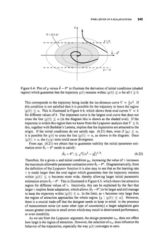
![246 ADAPTIVEAPPROXIMATION:
MOTIVATION
AND ISSUES
------ -- -
0*
I y=-a
Figure 6.5: Plot of y versus 8 - O* to illustrate the effect of the adaptation rate parameter
y on the set of initial conditions which guarantee that the trajectory y ( t ) remain within
ly(t)i 5 a for all t 2 0.
Finally, it should be noted that the above arguments are based on deriving su$-
cient conditions under which it is guaranteed that the trajectory does not leave the
approximation region {y I Iy(t)l 5 a}. However, the derived conditions are by
no means necessary conditions. Indeed, it can be readily verified that it is possible
for the unknown nonlinearity (modeling uncertainty) to steer the system towards the
n
stability region even if the inequality (6.22) is not satisfied.
The conditionsderived above forthe case ofa scalarparametric approximator can readily
be extended to the more realistic case of a vector parametric estimate, which yields the
following inequality for the initial conditions
(6.23)
1 1 . 1 2
-9;
2 + Z(eo -e*)Tr-l(io
- e*) 5 -a
2 .
Using the inequality [99]
we obtain that the initial parameter estimation error needs to satisfy the following inequality
to guarantee that iy(t)i 5 a for all t 2 0 :
(6.24)
Similarconclusions apply to the learning rate matrix r as applied to the scalar parameter y.
Trajectories Outside the Approximation Region. So far we have considered what hap-
penswhentheplantoutput y(t) remainswithin the approximationregionV = {y 1 lyl <a }
and under what conditionsit isguaranteed that y(t) E V.Next, we investigate what happens
if y ( t ) leaves the region V.
From eqn. (6.18) it is easy to see that if the MFAE, denoted by Ef(y), outside the
approximation region V grows faster than a certain rate then the trajectory may become
unbounded. For example, if Bf(y) = key outside of V,
where k, > a,, then the derivative
V of the Lyapunov fimction becomes positive. This implies that at least one (and possibly
both)ofthetwovariables iy(t)i2and lQ(t)l2= le(t)-e*12growswithtime. Itisimportant](https://image.slidesharecdn.com/adaptive-approximation-based-controlcompress-230219164415-f6eb4a64/85/adaptive-approximation-based-control_compress-pdf-264-320.jpg)
![STABILIZATIONOF A SCALAR SYSTEM 247
to note that if y ( t ) moves further away from the approximation region, naturally the ap-
proximation capability of the network may become even worse, possibly leading to further
instability problems. The reader may recall that in the case of localized basis function (see
Chapter 2) the approximation holds only within a certain region, and beyond this region the
approximator gives a zero, or some other constant, value.
To derive some intuition, let us consider the case where lGj(y)l 5 k, for lyI > 01 and,
as before, it assumed that lGj(y)i = 0 for Iy1 Ia. Therefore, when /yI > Q, V satisfies
V I-urny2 +keIvI,
which implies that for Q < /y/2 ke/urn(for the time being we assume that cy < &/urn),
the Lyapunov derivative satisfies V 5 0, while for 1y/ < ke/um,the Lyapunov derivative
is indefinite (can be positive or negative). This observation, combined wjth the assumption
that for IyI I a, the approximation error (MFAE) is zero and thus V 5 0, yields the
following general description for the behavior of the Lyapunov function derivative:
Another key observation regarding the stability properties is that during time periods
when V is indefinite there is nothing to prevent the parameter estimation error 6(t)from
growing indefinitely. Specifically, if lyi 5 k,/urn and 8(t)does not satisfy the inequality
(6.24) then it is possible for 181 -+ 03. This type of scenario was encountered earlier
in Chapter 4, where it was referred to as parameter drift. As discussed in that chapter,
parameter drift can be prevented by using so-called robust adaptive laws as described in
Section 4.6. If we use the projection modification in this case, we can guarantee that
ie(t)l 5 ern,where 8, is the maximum allowed magnitude for the parameter estimate.
As we saw earlier in Chapter 4,with the projection modification the closed-loop stability
properties are retained if 8, is large enough such that 16'1 5 Om.
The stability properties are illustrated in Figure 6.6 for the case where both y and 8
are scalar. The dark shaded region R1corresponds to the asymptotic stability region
that guarantees that y ( t ) + 0. In other words, if the initial condition (yo,&) E R
1
(or if at some time t = t', we have (y(t*),e(t*))E R1, then it is guaranteed that the
trajectorywillremaininR1 andlimt,, y(t) = 0. Thepropertythat (yo, $0) E R
1implies
( y ( t ) ,e(t))E 72.1 for all t 2 0 makes R
1apositively invariant set [134]. If (yo, 40) E R
2
or (yo,6,) E 72.3 (medium shaded region), then the Lyapunov function derivative V is still
negative semidefinite; however, in this case the trajectory may go into R
q (lightly shaded
region), where V is indefinite (can be either positive or negative). For example, a trajectory
that starts in Rzmay go to R1,or it may go to 724. From 72.4 (indefinite region) it may go
to R3,it may go back to Rz,
or it may even go to 721. In summary, a trajectory in R
1will
remain there and cause y(t) to converge to zero, while a trajectory in R
zuR
3 uR
q will
remain bounded but it may not go to the convergent set R1.
From the diagram, assuming that Iy(0)l < Q and 8 < em,we see that the maximum
value that y ( t ) can take (let us refer to it as gm; i.e., Iy(t)i I ym for all t 2 0), can be
obtained by looking at the Lyapunov curve passing through the point (y,6) = (ke/urn*
e),
where eis given by
e= ma~{8,,,- e*, -em - e*).](https://image.slidesharecdn.com/adaptive-approximation-based-controlcompress-230219164415-f6eb4a64/85/adaptive-approximation-based-control_compress-pdf-265-320.jpg)
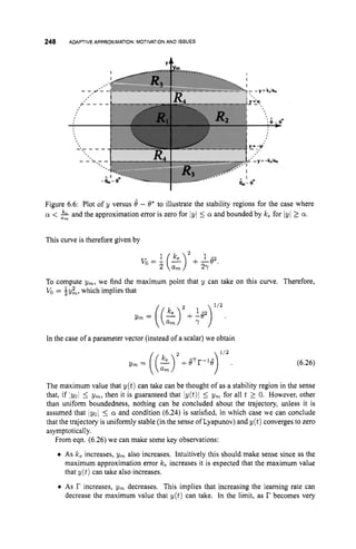
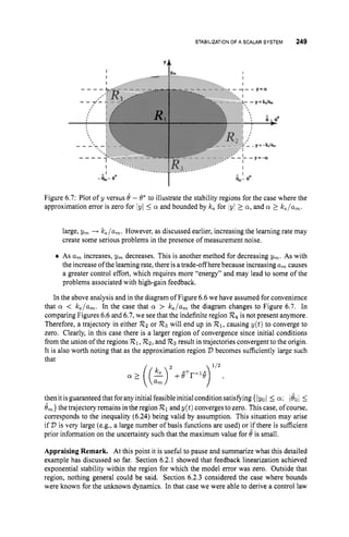
![ADAPTIVE APPROXIMATIONBASED TRACKING 257
which implies that V 5 u,e2 = 2a,V. Therefore, the tracking error e(t)= y(t) - yd(t)
converges to zero exponentially fast. If the assumed bounds on the uncertainty are global,
then the stability results will also be global.
The algebraic singularity introduced by the definition of vg(y, e,u ) can be eliminated as
follows. The control law of eqn. (6.41)can be rewritten as
u,
u =
go(Y) +v g (Y.e, u a ) '
where the intermediate control variable u, is given by
'% = - h e +$d - fo(y) - v
U
f (3'. e ) ,
Since go(y) +vg is assumed to be positive for all y (for stabilizability purposes), the sign
of u is the same as the sign of u,. Therefore the definition of wg(y,e. u) can be modified
as follows without losing any of the stability properties, and at the same time eliminating
the algebraic singularity:
(6.45)
The above feedback control law is, in general, discontinuous at e = 0 and at u, = 0. This
may cause chattering at the switching surfaces. As discussed earlier, this problem can be
remedied by using a smooth approximation of the form described by eqn. (6.9),as shown
diagrammatically in Figure 6.3. As before, the main idea is to create a smooth transition of
vf and wg at the switching surfaces e = 0 and u, = 0. In this case, the design and stability
derivation is a bit more tricky because the bounds f ~ ,
fu,
gL, and gu are functions of y
while the switching is a function of the tracking error e(t)and the signal u,.
EXAMPLE6.5
Consider the scalar system model
c = f*(Y) + (90+g*(y))u
where the only available apriori information is go = 2 and
-Y2 5 f*(y) 5 Y2
for all y E 9
'
.
The feedback control specification is to track reference inputs yc(t)
with bandwidth up to 2 and reject initial condition errors with a time constant of
approximately 0.1 s.
For the tracking control design process we require a reference trajectory yd(t) and
its derivativeIjd (t).If the derivativeof ycis not available, then as discussed in Section
A.4, we can design a prefilter with yc(t) as its input and [ y d ( t ) %
y d ( t ) ] as outputs. To
ensure that the error between yd(t) and yc(t) is small, the prefilter should be stable,
with unity gain at low frequencies, and with bandwidth of at least 2 y.
Such a
prefilter, as discussed in Example A.9 of Section A.4, is given by
[ ::] = [-I: -2.:] [::I+[ :Iyc (6.46)
(6.47)
[;:I = [t :I[::]](https://image.slidesharecdn.com/adaptive-approximation-based-controlcompress-230219164415-f6eb4a64/85/adaptive-approximation-based-control_compress-pdf-275-320.jpg)
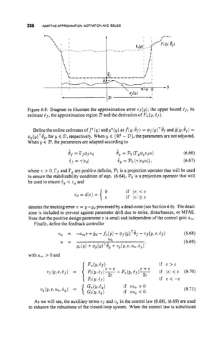
![ADAPTIVEAPPROXIMATION
BASED TRACKING 273
2. -5
l
:
0 2 4 6 8 10 12 14 16 18 20
-10
0 2 4 6 8 10 12 14 16 16 20
4 1 I
I I
0 2 4 6 6 10 12 14 16 18 20
-4 1
time, t s
Figure 6.9: Simulation performance of the bounding controller described in Example 6.5.
The output is y. The tracking error is e = y - Y d . The control signal is u.
of the controller with a sampling time T, and zero-order-hold control signalsbetween
the sampling instants showed very large magnitude switching in the control signal
for T, > 0.005 s.
Variables indicating the performance of the approximation based controller of
Example 6.7 are show in Figyes 6.10-6.13. For implementation of this controller,
the approximation fknctions f and g are each implemented using normalized radial
basis functions using
with centers located at c, = -10.0 +z for z = 0. .. . .20. Initially, Of = Og = 0.0.
For function approximation by eqn. (6.66) the learning rates were I
?
, = rg= 1001.
For bound estimation by eqn. (6.74), = 1.0 and of = og = 1.0. Figure 6.10
shows the output y(t), tracking error e(t),and control signal u(t)for the first 20 s
of the simulation. This figure is included to show that the initial tracking error and
control signal transients are reasonable. Note that the tracking error significantly
exceeds the dead-zone (E = 0.05).Therefore, function approximation is occumng.
Figure 6.11 shows the output y(t), tracking error e(t),and control signal u(t)for
t E [80.100].
This figure show that as learning progresses. the increased function
approximation accuracy results in improved control performance as exhibited be the
decreased tracking error. Note that for the majority of the time shown in Figure
6.11,the tracking error is within the dead-zone lyl < c^ = 0.05 for which parameter
adaptation no longer occurs. Only for short time intervals at specific ranges of y does
the tracking error leave the dead-zone. Therefore, function approximation only is still
occurring at those specific ranges of y. If the simulation were continued for a longer
duration the tracking error would ultimately enter and remain in the dead-zone. The](https://image.slidesharecdn.com/adaptive-approximation-based-controlcompress-230219164415-f6eb4a64/85/adaptive-approximation-based-control_compress-pdf-291-320.jpg)
![274 ADAPTIVEAPPROXIMATION:
MOTIVATION
AND ISSUES
approximated functions are plotted at 10-sintervals in Figure 6.12. In this figure, the
actual functions f *and g" are shown with dotted lines. The function approximation
errors are shown in Figure 6.13. Several features of these figures are worth noting.
1. The initial f(y) = 0. The subsequent sequence of approximated functions is ordered
from top to bottom at y = -9.
2. The initial g(y) = 0. The subsequent sequence of approximated functions is ordered
from bottom to top at y = -6.
3. Astimeprogresses andtraining samplesare accumulated, the approximated functions
appeartoconvergetoward f
' and9'. However, this shouldbeinterpreted with caution
since the analysis guaranteed boundedness, but not convergence of the approximator
parameters. Note for example that for the t = 10plot of the functions that while the
approximation error for 4 has decreased at jyl = 2 it has increased at y = 0.
4. As time increase, the approximation error for lyI E [9,10]is increasing. This is
due to the fact that very few training samples are available in that range. However,
these parameters are not diverging. Instead, the parameters are beingjointly adjusted
to approximate the functions using the available training samples. Throughout the
process, the Lyapunov function is decreasing.
These Simulink results were achieved using a maximum step size of 0.005 s and
the default relative tolerance of le-3. A discrete-time implementation using a zero-
order-hold control signal between control samples computed 1OOHz yield essentially
n
identical performance to that shown in Figures 6.10-6.13.
Bounding Function Development. So far, we have estimated parameters E f and Eg that
bound the function approximation error over the entire region 2
7
.In some applications,
it is of interest to estimate functions that bound lef(y)I and leg(y)l over the entire region
V.When this is the case, we define df(y) = q!~;@(y) and Zg(y) = $T@(y) where each
element of each vector $ f and Gg is positive. Define @
; and $I,* as the vectors with the
smallestelementssuchthat ief(y)i 5 ($I;)T~(y) and leg(y)l 5 ($:)TC$(y) foranyy E 2
)
.
Then, we can change eqn. (6.74) to
for y E V and i = 1... . ,N . With these changes, both the Lyapunov function and its
derivative analysis will change, but the underlying ideas are the same.
Consider the Lyapunov function
The time derivative is](https://image.slidesharecdn.com/adaptive-approximation-based-controlcompress-230219164415-f6eb4a64/85/adaptive-approximation-based-control_compress-pdf-292-320.jpg)
![ADAPTIVEAPPROXIMATIONBASED TRACKING 275
0 0
-0 2
-0 4
0 2 4 6 8 10 12 14 16 18 20
-4 1 J
0 2 4 6 8 10 12 14 16 18 20
time. 1, sec
Figure 6.10: Initial simulation performance of the approximation based controller described
in Example 6.7. The output is y. The tracking error is e = y -yd. The control signal is u.
-0.2 1 I
80 82 E4 86 88 90 92 94 96 98 100
-4 ' I
80 82 84 86 88 90 92 94 96 98 100
time, 1. sec
Figure 6.11: Simulation performance of the approximation based controller described in
Example 6.7 for t E [80,100]. The output is y. The tracking error is e = y - yd. The
control signal is u.](https://image.slidesharecdn.com/adaptive-approximation-based-controlcompress-230219164415-f6eb4a64/85/adaptive-approximation-based-control_compress-pdf-293-320.jpg)
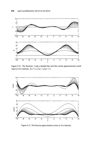
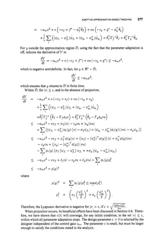
![278 ADAPTIVE APPROXIMATION:MOTIVATION AND i s s m
6.4 NONLINEAR PARAMETERIZEDADAPTIVE APPROXIMATION
The differences and trade-offs between linearly and nonlinearly parameterized approxima-
tors were discussed in Chapter 2. In the case of linearly Parameterized approximators, the
parameters o are kept fixed, therefore f^(y;0,o) = @(y;u)TOcan be conveniently written
as
where the dependence of q5 on the fixed o vector can be dropped altogether. The synthesis
and analysis of adaptive approximation based control systems developed so far in this
chapter, were based on linearly parameterized approximators. In this section, we consider
the case of nonlinearly parameterized approximation models and derive adaptive laws for
updating not only the 0 parameters of the adaptive approximators but also the u parameters.
Let us consider the adaptive approximation of the unknown function f*(y) by a non-
linearly parameterized approximator. For notational convenience, define w := [BT oTlT.
We have
f^b;
030) = OT@(Y) = 4(y)TQ
f*(Y) = f^(y;w*)+Zf(Y)
= f ( y ;w)+ [h
w*)
- f ( y ;w
)
]+Ef(Y) (6.76)
where ef(y) is the MFAE and w*is the optimal weight vector that minimizes the MFAE
within a compact set V,
which typically represents the approximation region (see Section
3.1.3).
If we assume that f(y; w)is a smooth function with respect to w then using the Taylor
series expansion f(y; w")
can be written as
f^(y;w*) = f^(y;w-G)
(6.77)
where .W := w - 20* is the parameter estimation error and F ( y ; w)represents the higher-
order terms off with respect to w.
Before proceeding with the analysis using eqn. (6.77), let us examine the properties of
the higher-order term F.Using the Mean Value Theorem [64], it can be shown that
a?
f(y: w)- -(y; w)G -F(y;w).
aw
=
I n Y ; Ul)l IPb;w)llGll
where
and [w,
w*]
is a line segment connecting w and w*;
i.e.,
[w,
w*]
:={x 1 x = xw +(1 - X)w*; 05 x 5 l}.
It is noted that based on the definition ofp(y;w), the following property holds:
lim p(y:w) = 0 Vy E V.
W
'
W
'
Therefore,](https://image.slidesharecdn.com/adaptive-approximation-based-controlcompress-230219164415-f6eb4a64/85/adaptive-approximation-based-control_compress-pdf-296-320.jpg)

![286 ADAPTIVEAPPROXIMATION
BASED CONTROL:GENERAL THEORY
systems,we firstconsider the ideal case where the uncertainties can be approximatedexactly
by the selected approximation model within a certain operating region of interest (i-e.,the
Minimum Function Approximation Error (MFAE) is zero within a certain domain D),and
then we consider the case that includes the presence of residual approximation errors and
disturbances. The latter case is referred to as robust adaptive approximationbased control.
As we will see, to achieve robustness, we utilize a modification in the adaptive laws for
updating the weights of the adaptive approximation. This modification in the adaptive
laws is based on a combination of projection and dead-zone- techniques that have been
introduced in Chapter 4, and also used in Chapter 6.
It is important to note that this chapter follows a structure parallel to that of Chap-
ter 5, where we introduced various design and analysis tools for nonlinear systems under
the assumption that the nonlinearities were known. In this chapter, we revisit these tech-
niques (e.g., feedback linearization, backstepping), with adaptive approximation models
representing the unknown nonlinearities.
7.1 PROBLEM FORMULATION
This section presents some issues in the problem formulation for adaptive approximation
based control. As we will see, certain notation, assumptions, and control law terms will be
used repeatedly throughout this chapter. To decrease redundancy throughout the following
sections, these items and their related discussion are collected here.
7.1.1 TrajectoryTracking
Throughout this chapter, the objective is to design tracking controllers such that the system
output y(t) converges to Y d ( t ) as t -+ o.
The controller may use the derivatives y i )(t)for
i = 1,....n. As discussed in Appendix A.4, these signals are continuous, bounded, and
available without the need for explicit differentiation of the tracking signal.
Associated with the tracking signal gd(t), there is a desired state z d ( t ) of the system,
which is assumed to belong to a certain known compact set V for all t > 0. In feedback
linearization control methods it will typically be the case that the i-th component of the
desired state satisfies: xd, (t)= y
:
-
l
) (t).where gf'(t) = &(t).In backstepping control
approaches, the desired state is defined by certain intermediate control variables, denoted by
a,.The tracking error between zd, (t)and z, (t)will be denoted by 5,
(t)= z, (t)-xd, (t).
The vector of tracking errors is denoted as Z = [&. ... 2n]T.
7.1.2 System
Throughout this chapter, the dynamics of each state variable may contain unknown func-
tions. For example, the dynamics of the i-th state variable may be represented as
where z, can be the control variable u or the next state z,+1. The functions fo, (z) and
go,(z)are the known components of the dynamics and f,"(x)and g: (z)are the unknown
parts of the dynamics. Both the known portion of the dynamics, fo, (z)and go,(z),and the
unknown functions f: (z)and g: (z)are assumed to be locally Lipschitz continuous in z.
The unknown portions of the model will be approximated over the compact region V.
This region is sometimes referred to as the safe operating envelope. For any system, the](https://image.slidesharecdn.com/adaptive-approximation-based-controlcompress-230219164415-f6eb4a64/85/adaptive-approximation-based-control_compress-pdf-304-320.jpg)
![APPROXIMATION
BASED FEEDBACK LINEARIZATION 289
scalar system, which is a first step in the design of feedback linearization. Specifically, in
Section 6.3.5 we considered the tracking problem for a scalar system and investigated the
key issues encountered in the use of adaptive approximation based control.
In this section we consider the feedback linearization problem with unknown nonlin-
earities, which are approximated online. We start in Section 7.2.1 with a scalar system
(similar to Chapter 6) in order to examine carefully the ideal case, the need for projection
and dead-zone techniques, and the robustness issues that are involved. In Section 7.2.2 we
consider adaptive approximation based controlof input-state feedback linearizable systems,
and in Section 7.2.3 we consider input-output feedback linearizable systems.
7.2.1 Scalar System
The simple scalar system
x = (fo(x) +f*(z))
+ (go(.) +g*(z))u. (7.5)
y = x (7.6)
has already been extensively discussed in Chapter 6. To achieve tracking of yd by y, the
approximation based feedback linearizing control law is summarized as
(7.9)
(7.10)
where 2 = x -yd is the tracking error, a, > 0 is a positive design constant, rfand r, are
positive definite matrices, and Ps is the projection operator that will be used to ensure the
stabilizability condition on 8,. The auxiliary terms vf and v, are included to ensure that
the state remains within a certain approximation region 'D, see Section 7.2.4.
Theorem 7.2.1 summarizes the stability properties for the adaptive approximation based
controller in the ideal case where the MFAE is zero and there are no disturbance terms.
Theorem 7.2.1 [Ideal Case] Let T J ~
and ug be zerofor IC E V and assume that df, @
, are
bounded. In the ideal case where the MFAE and disturbances are zero, the closed-loop
system composed o
f the system model (7.5) with the control law (7.7)-(7.10) satisfies the
following properties:
0 2, x,ef,e, E c,
0 i E C 2
0 5(t)--+ 0 as t --$ 02.
Proof: Outside the region 'D, we assume that the terms u f and vy have been defined to
ensure that the state will convergeto and remain in 'D(i.e., the set 2)is positively invariant).
Therefore, the proof is only concerned with x E 2).
For 5 E '
D with the stated control law, after some algebraic manipulation, the dynamics
of the tracking error 5= y - yd reduce to](https://image.slidesharecdn.com/adaptive-approximation-based-controlcompress-230219164415-f6eb4a64/85/adaptive-approximation-based-control_compress-pdf-307-320.jpg)
![290 ADAPTIVEAPPROXIMATIONBASEDCONTROL: GENERAL THEORY
The derivative of the Lyapunov function
v = 1(52 +ejr;lef +
2
satisfies
(7.11)
Therefore, with the adaptive laws (7.9),(7.10), the time derivative ofthe Lyapunov function
V becomes
v = -a,?'
when the projection operator is not enforcing the stabilizability condition. Note that as long
as $f, 4, are bounded, Lemma A.3.1 completes the proof. When the projection operator is
active, as discussed in Theorem 4.6.1, the stability properties of the control algorithm are
preserved. rn
The previous theorem considered the ideal case. The following theorems analyze two
possible approaches applicable to more realistic situations, where we consider the presence
of disturbance terms and MFAE.
Consider again the system described by (7.5) with the addition of another term d(t),
which may represent disturbances:
j . =
=
fo(x) +f
*
(
.
) +(
g
o
(
.
) +g*(.))u +d
fo(.) +$;8; +(go(.) +$,T&)u +6f +6 , ~
+d
= f
o
(
.
) +4;e; +(
g
o
(
.
) +O,T8;;)u
+6
where 6 is given by
6(x,u,t )= 6f(")+b,(z)u +d.
(7.12)
As discussed earlier, the first two terms of 6 represent the MFAE, which arise due to the
fact that the corresponding adaptive approximator is not able to match exactly the unknown
functions f* and g
' within the region D.
Theorem 7.2.2 [Projection] Let ufandv, be zerofor 2 E 2
3 andassume that $f, 4
, are
bounded. Let theparameter estimates be adjusted according to
e j = ~ B ( r j $ f ~ ) ,
for x E D (7.13)
4, = PSB (rg$,zu): for x E D (7.14)
where P, is a projection operator designed to keep 9 j in the convex and compact set Sf
and P ~ B
is a projection operator designed to keep 6, in the convex and compact set S,,
which is designed to ensure the stabilizability condition, the condition that 0: E S
,
,and
the boundedness of 8,.
1. In the case where b = 0,
5,2, e,, e, E c,
5 E C z](https://image.slidesharecdn.com/adaptive-approximation-based-controlcompress-230219164415-f6eb4a64/85/adaptive-approximation-based-control_compress-pdf-308-320.jpg)
![APPROXIMATIONBASEDFEEDBACKLINEARIZATION 291
0 5(t)---t 0 us t + m.
2. In the case where 6# 0,but 1
6
15 60 where 60i
s an unknownpositive constant, then
2,5,8f,g,, 8f,8, E C
,
.
Proof:
Theorems 4.6.1 and 7.2.1,and therefore it is not included here.
5 = y - Yd reduce to
The time derivative of the Lyapunov function of eqn. (7.11)becomes
The proof of the case where 6 = 0 is straightforward based on the proofs of
For 6 # 0, for 2 E D,with the stated control law, the dynamics of the tracking error
.
5= -arn$ - eT
-f @f -@J,U +6.
Using (7.13)and (7.14) the time derivative of the Lyapunov function becomes
V = -am?’ +56,
if the projection modification is not in effect. In the case that the projection is active,
then, as shown in Theorem 4.6.1,the stability properties are retained (in the sense that the
additional terms in the derivative of the Ly!pu?ov function are negative) and in addition it
is guaranteed that the parameter estimates Of,8, remain within the desired regions S f and
S,, respectively. Therefore, with the projection modification, we have
V 5 -a,z2 +5
.
6
.
We note that as 1
5
1 increases, at some point the term -a,Z’ +5
6 becomes negative.
Therefore, 5 E C
,
. When a
,
?
? < 65,
the time de_rivative_ofthe Lyapunov function may
become positive. In this case, the parameter errors 8fand 8, may increase (this is referred
tp as parameter drift); however, the projection on the parameter es,tim,ates_will maintain
Of E S f and 8, E S,. By the compactness ofSf and S,, we attain Of,Qg, Of,8, E C,.
So far we have established that 5,
6f gg are bounded; however, it is not yet clear what
is an upper bound or the limit for 5,which is a key performance issue. Consider the TWO
cases:
1. If a,Z2 < 65,
then 8fand Jg may increase with either 8f + aSf or 8, + as,,
where 85, and as, denote the bounding surfaces forSf and S,, respectively. While
this case remains valid, we have a
,
& < 1
6
1 < 60;
however, a change in @f or #g
may cause the state to switch to Case 2 at any time.
2. With a
,
5
’ 2 65,the time derivativeofthe Lyapunov function is decreasing. Let the
condition a
,
*
’ L 65be satisfied fort E [ts,,tf,]
with 1
5(t6%)/
= 1
5(tf,)l = &.
Fort in this interval,
(7.15)](https://image.slidesharecdn.com/adaptive-approximation-based-controlcompress-230219164415-f6eb4a64/85/adaptive-approximation-based-control_compress-pdf-309-320.jpg)
![292 ADAPTIVEAPPROXIMATIONBASEDCONTROL GENERALTHEORY
Since S is bounded and Xd is bounded, then x is also bounded.
Note that there is no limit to the number of times that the system can switch between cases
1 and 2. The fact that S(t)becomes small for an extended period of time (i.e., Case 1)
does not guarantee that it will stay small. Parameter drift or changes in the reference input
may cause the system to switch from Case 1 to Case 2. The bound B applicable in Case 2
may be quite large as it is determined by the maximum value achieved over the allowable
parameter sets. The term “bursting” has been used in the literature [5, 114, 119, 1581 to
describe the phenomenon where the tracking error d is small in Case 1, and while it appears
to have reached a steady state behavior, there occurs a switch to Case 2, which results in S
increasing dramatically. In summary, the best guaranteed bound for this approach is given
rn
The previous result and the proof highlights the fact that merely proving boundedness is
not necessarily useful in practice. From a designer’s viewpoint, it is important to be able
to manipulate the design variables in a way that improves the level of performance. The
bound provided by (7.15) is not useful from a designer’s point of view since it cannot be
made sufficiently small by an appropriate selection of certain design variables.
In the next design approach, we introduce a dead-zone on the error variable and investi-
gate the closed-loop stability properties of this new scheme.
Theorem 7.2.3 [Projectionwith Dead-Zone] Letvf andv, bezeroforx E V andassume
that 4J , 4, are bounded. Let theparameter estimates be adjusted according to
by eqn. (7.15) and this bound is not small.
er = pB (rf4fd(z,E)), for z E v (7.16)
4, = PSB (rg4,d (5,E ) u ) for z E v (7.17)
where
and
60
E = - + p
am
for some p > 0. PBisaprojection operatordesigned tokeep 6, in the convexand compact
set S f and Ps, is aprojection operator designed to keep 6, in the convex and compact set
S,, which is designed to ensure the stabilizability condition, the condition that $9’ E S,,
and the boundedness of 6,. In the case where 1
6
1 < 60,
1. 3, 5,e,, e, E L
,
;
2. S is small-in-the-mean-square sense, satisfying
3. d(t) is unyormly ultimately bounded by E; i.e., the total time such that lS(t)1 > E is
jnite.
Proof: Let the condition Id(t)i > E be satisfied for t E (ts,,t ~ % ) ,
i = 1,2,3,..., where
t y , < tf. 5 t,%+,,
/S(t)l 5 E for t E (t~,,t~,+~),
t,, is assumed to be zero without](https://image.slidesharecdn.com/adaptive-approximation-based-controlcompress-230219164415-f6eb4a64/85/adaptive-approximation-based-control_compress-pdf-310-320.jpg)
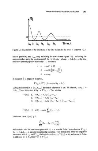
![294 ADAPTIVEAPPROXIMATIONBASED CONTROL:GENERALTHEORY
Using the inequality
1
XY I a2x2+g 2 , va # 0,
we have that
where a2 = am/2. Therefore, we obtain
v 5 - a m 5 2 + -
6
,
.
1 2 (7.18)
2 2am
Integrating both sides of (7.18) over the time interval [t,t +T ]yields
Hence
t+T
which completes the proof.
In this case, where I6(t)I 5 60for all t > 0, then the ultimate bound for the tracking error
is Z(t)l 5 E. In practice, it is usually not desirable to decrease the bound by increasing
am, since this parameter is directly related to the magnitude of the control signal (see eqn.
(7.7)) and the rate of decay of transient errors. Instead, the designer can consider whether it
is possible to decrease 60.If60 was determined by disturbances, then not much can be done
-unless the general structure of the disturbance is already known. If 60was determined by
unmodeled nonlinear effects, then the designer can enhance the structure of the adaptive
approximator.
One of the possible disadvantages of the dead-zone is the need to know an upper bound
60on the uncertainty. However, if the designer utilizes a smaller than necessary 60 which
results in the inequality I6(t)1 5 60not being valid for some t > 0, then the stability result
is essentially the same as for Theorem 7.2.2. This is left as an exercise (see Problem 7.1).
7.2.2 input-State
To illustrate some of the key concepts andto obtain some intuitionregarding the control and
robustness design, in Section 7.2.1, we considered the scalar case. In this subsection we
consider the n-th order input-state feedback linearization case. In Section 7.2.2.1, we first
consider the ideal case where the MFAE and disturbances are all zero. In Section 7.2.2.2,
we consider an approach to achieve robustness with respect to these same issues.](https://image.slidesharecdn.com/adaptive-approximation-based-controlcompress-230219164415-f6eb4a64/85/adaptive-approximation-based-control_compress-pdf-312-320.jpg)
![296 ADAPTIVE APPROXIMATION BASED CONTROL:GENERALTHEORY
In the ideal case where we assume that the MFAE is zero (i.e., there exists 0; such that
f*(z)
= @f(z)T8;for all z E V,
and correspondingly for 8;), then the control law defined
in (7.23) and (7.24) results in the following closed-loop tracking error dynamics
i = ( A- BKT)E - B@f(;Z)T8f
- B @ , ( Z ) ~ ~ , U . (7.27)
Since the feedback gain vector K is selected such that A - BKT is Hunvitz, for any
positive definiteQ there exists a positive definite matrix P satisfyingthe Lyapunov equation
P ( A- BKT) +(A - BKT)TP= -Q. (7.28)
In the following, without any loss of generality we will select Q = I. Finally, based on the
solution ofthe Lyapunov equation, we define the scalar training error e(t)as follows:
e = BTP?.
The stability properties of this control law are summarized in Theorem 7.2.4.
Theorem 7.2.4 [Ideal Case] Let vf and vy be zerofor z E V and assume that Q f , 4
,
are bounded. In the ideal case where the MFAE and disturbances arezero, the closed-loop
system (7.19)-(7.21) with the control law (7.23)-(7.26)satisfies thefollowingproperties:
- A
b 2, 5, Of, 8, E c
,
? € I 2 2
E ( t ) -+ 0 as t -+ 00.
Proof: Outside the region V, we assume that the terms wf and ug have been defined
to ensure that the state will converge to and remain in V.Therefore, the proof is only
concerned with z E 2
)
.
For z E V,
the time derivative of the Lyapunov function
v = Z ~ P E
+e,Tr;lGf +e,Tri18, (7.29)
satisfies
for Q = I . Therefore, with the adaptive laws (7.25)-(7.26), the Lyapunov time derivative
V becomes
i/ = -ET&
which is negative semidefinite. In the case that the projection operator Psbecomes active
in order to ensure the stabilizability condition, as discussed earlier, the stability properties
are preserved. Therefore, V satisfies V 5 -dT5 for all z E V.Hence the application of
The above design and analysis of approximation based input-state feedback linearization
was developed for nonlinear systems of the companion form (7.19H7.21). This can be
extended to a more general class of feedback linearizable systems of the form
Lemma A.3.1 completes the proof.
X = AX+BP-'(z) [U - ~ ( z ) ] , (7.30)](https://image.slidesharecdn.com/adaptive-approximation-based-controlcompress-230219164415-f6eb4a64/85/adaptive-approximation-based-control_compress-pdf-314-320.jpg)
![APPROXIMATIONBASED FEEDBACK LINEARIZATION 297
where uis a scalar control input, z is an n-dimensional state vector, A is an n x R matrix,
B is an n x 1matrix, and the pair (A,B )is controllable. The unknown nonlinearities are
contained in the continuous functions LY : Xn H !
J
?
l and /
3 : XnH X1, which are defined
on an appropriate domain of interest V,
with the function p(z)assumed to be nonzero for
everyx E V.It is noted that the caseofsystems ofthe form (7.30)withknownnonlinearities
was studied in Section 5.2. The tracking control objective is for z(t)to track the desired
state zd(t),where X d ( t ) is generated by the reference model
X d = AXd +Br, (7.31)
and r(t)denotes a certain command tracking signal (see Appendix Section A.4). Using the
definition 1= z - Q, the tracking error dynamics are described by
k = A? +B [p-'(x) (u - a
(
.
)
) - r].
These tracking error dynamics can be written in the form (similar to (7.22)):
k = A5 +B ((fo(z)
+f*(x))+ (
g
o
(
.
) +g*(z))u- d t ) ) (7.32)
where
fo(z)
is the known component of -p-'(z)cy(z);
f*(z)is the unknown component of -P-l(x)a(x);
g
o
(
.
) is the known component of p-'(x);
0 g*(x)is the unknown component of P-l(z).
Note that the command signal r(t)corresponds to the signal yy'(t) that was used for the
nonlinear system in companion form.
Once the tracking error dynamics are formulated as in eqn. (7.32), the approximation
based feedback controller (7.23)-(7.26), with yP)(t) being replaced by r(t),can be used
to achieve the tracking results described by Theorem 7.2.4.
In the next subsection, we consider the case where the adaptive approximators cannot
match exactly the unknown nonlinearities within the domain of interest V (i.e., the MFAE
is nonzero), and there may be disturbance terms.
7.2.2.2 Robustness Considerations. In arealistic situation, therewill bemodeling
errors. If the modeling error, represented by 6,satisfies a matching condition. then the
tracking error dynamics satisfy
= AE +B (fo(z)
+f*(x)+(
g
o
(
.
) +g*(x))u - yp)(t)) +B6.
As previously, the term 6(t)may contain disturbance terms, as well as residual approxima-
tion errors due to the MFAE, which was discussed earlier. The following theorem presents
a projection and dead-zone modification in the adaptive laws of the parameter estimates
that ensures some key robustness properties.
Theorem 7.2.5 [Projectionwith Dead-Zone] Letvf andv, bezeroforx E V andassume
that of,
Q
, are bounded. Let theparameter estimates be adjusted according to
Jf = Ps(rfOfd(e.z,E)). for X E V (7.33)
6, = PsS (r,qgd(e.E,E)u), for 3: E V (7.34)](https://image.slidesharecdn.com/adaptive-approximation-based-controlcompress-230219164415-f6eb4a64/85/adaptive-approximation-based-control_compress-pdf-315-320.jpg)
![298 ADAPTIVE APPROXIMATIONBASEO CONTROL: GENERAL THEORY
wherefor P satisfying eqn. (7.28)
(7.35)
E = 2IIPq260 + P (7.36)
where p > 0 is a positive constant, and X p and are the maximum and minimum
eigenvalues of P respectively. PB is a projection operator designed to keep 8, in the
convex and compact set Sf and PSBis a projection operator designed to keep 8, in the
convex and compact set S,, which i
s designed to ensure the stabilizability condition, the
condition that 0; E S,, and the boundedness of 8,. In the case where 1
6
1 < SO,
1. e, x,Of, 8, E c
,
;
2. 2 is small-in-the-mean-square sense, satisfiing
3. !2(t)112 is uniformly ultimately bounded by E; i.e., the total time such that 5TP2>
Proof: Outside the region D,we assume that the terms vf and v9 have been defined
to ensure that the state will return to and remain in D.Therefore, the proof will only be
concerned with x E D.
In the region D,
with P selectedto solve the Lyapunov eqn. (7.28) with Q = I , the time
derivative of the Lyapunov function (7.29) is
Xpa2 isjnite.
Supposethatthetime intervals (t,,,tft) aredefinedasdiscussed relativeto Figure 7.1, sothat
the condition 2(t)TP2(t) > Xpe2is satisfied only fort E (ts,,
tfL),z = 1,2,3,..., where
t,, < t f , I t,,,,. Since 2(tft)TP2(tfz)
= 5(tsz+,)TP2(t,z+,)
= Xpc2 and parameter
estimation is off fort E [tf%,
ts,+,],
we have that V(t,) = V(thL+,).When t E (t5",
t f z )
foranyi thefactthat2'PZ > XP (2/IPB1/2S0
+ P ) ~
ensuresthat 112112 > 21/PBl/2So+p;
therefore, when projection is not in effect,
V = -2T2+22TPB6
I -
1
1
2
1
1
; +211~ll2llPBIl21~1
I -ll2ll2 ( I I ~ I I Z- 211PBIl2~0)
I -&P.
Therefore, by integrating both sides over (ty,,
th),
V(tf%) 5 V(ts,) -&P (tf%
-t 5 % )
I
I
V(tf%_,)
-E P (tf. -t 3 , )
V(t,-*)- EP ((tf%
- L)
+ (tA-1 - t S J )](https://image.slidesharecdn.com/adaptive-approximation-based-controlcompress-230219164415-f6eb4a64/85/adaptive-approximation-based-control_compress-pdf-316-320.jpg)
![APPROXIMATIONBASEDFEEDBACKLINEARIZATION 299
Hence, since V(tf%)
2 0,
which shows that the total time spent with I T P I >
1,2,3,.. .isapositivedecreasingsequence, eitherthisisafinitesequenceorlimi,, V(tfL)=
V
, exists and is finite. In addition, ift > t f h ,
then V ( t )< V(tf*).
is finite. In addition, V(t,) i =
Within the dead-zone, it is obvious that XpliZiil 5 fTP55 X ~ E ~
implies
Outside the dead-zone, using the inequality,
1
xy 5 p2x2+- V’P#O,
4 P Y ’
we have that
for p2 = 0.5. Integrating both sides of the last equation over the time interval [t,t +T ]
we obtain
Therefore,
X P 2
XP
t f T
4 115(r)Il;d r 5 2V(t) +c2T 5 2V(t) + -E T,
which completes the proof. W
The mean-square and the ultimate bound E are increasing functions of the bound 60 on
the model error. When the model error is determined predominantly by the MFAE, the
performance can be improved, independent of the control parameters K ,by increasing the
capabilities of the adaptive approximator, which decreases 60.](https://image.slidesharecdn.com/adaptive-approximation-based-controlcompress-230219164415-f6eb4a64/85/adaptive-approximation-based-control_compress-pdf-317-320.jpg)
![300 ADAPTIVEAPPROXIMATIONBASED CONTROL:GENERALTHEORY
Figure 7.2: Block diagram implementation of the trajectory generation prefilter described
in Section 7.2.2.3.
7.2.2.3 Detailed Example This subsection presents a simulation implementation of
the control approach of Section 7.2.2applied to the system
j
.
, = x 2
x.2 = x 3
x3 = f ( X 1 , az) +g(z1,22).
which is of the form of eqns. (7.19)-(7.21). The only knowledge o f f and g assumed at
the design stage is that both are continuous with -1 5 f 5 1 and 0.05 5 g. Therefore,
fo = go = 0. We also assume that the system is designed to safely operate over the region
The user of the system specifies a desired output r ( t ) that will be used to generate a
desired trajectory q ( t )= [ x d l (t)x d 2 (t)X d 3 (t)lTand x d 3 (t)such that x d is continuous;
t > 0. The trajectory generation system is defined by
(xi,~ 2 )
E 2,= [-1.3, 1.31 x [-1.3,1.3].
X d and i d 3 ( t ) are bounded; ?dl = X d 2 and X & = X d 3 ; and, ( a d 1 (t),
X d 2 ( t ) ) E D for all
x d l = X d 2
x d 2 = XdS
x d s = a1 (a2 [ a ( a 3 ( T s - - d l ) ) -x&] - x d 3 )
where r, = ~ ( r )
and u(.)
is that saturation function
1.3 if a > 1.3
x if 1
x
1 5 1.3
i-1.3 if x < -1.3.
u ( x )=
Figure 7.2 shows this trajectory generation prefilter in block diagram form. The signal
T, (t)is a magnitude limited version of ~ ( t )
that is treated as the commanded value of X d l .
The signal v(t)= a3(rs(t)
-%dl (t))
has the correct sign to drive z d l toward r,. The signal
z
1
, has the same sign as v,but its magnitude is constrained to [-1.3,1.3], so that it can be
interpreted as a desired value for x d z . By the design of the filter, (r,(t),
us(t))E D for
all t 1 0 and the filter is designed so that ( Z d l , x d z ) track (r6,
us). However, due to the
dynamics of the filter, tracking may not be perfect. If it is essential that the commanded
trajectory always remain in D, then the magnitude limits in the function a
(
.
)should be
decreased from iz1.3. We select the parameter vector [ a l ,a2,a31 = 19,3,1]. Within the
linear range of the trajectory generator, this choice yields the transfer functions
3 - 27
-
r s3 +9s2 +27s +27](https://image.slidesharecdn.com/adaptive-approximation-based-controlcompress-230219164415-f6eb4a64/85/adaptive-approximation-based-control_compress-pdf-318-320.jpg)
![APPROXIMATIONBASED FEEDBACKLINEARIZATION 301
3 - 27s
-
r s3 +9s2+27s +27
x d 27s2
3 =
r s3 +9s2+27s +27
which have three poles at s = -3. As long as r is bounded, the signal xy)will be bounded,
but it isnot necessarily continuous. Issues related tothe design of such trajectory generation
prefilters are discussed in Appendix Section A.4.
For 2 E 23, the adaptive approximation based controller is designed to satisfy the re-
quirements of Theorem 7.2.5. The control gain is selected as K = [l,3,3]which gives
A - B K = [ 0 1
0 0 y ]
1
-1 -3 -3
with A and B defined as in eqn. (7.22). The matrix A - BK is Hurwitz with all three
eigenvalues equal to -1. The matrix solving Lyapunov eqn. (7.28) with Q = I is
2.3125 1.9375 0.5000
P = 1.9375 3.2500 0.8125
10.5000 0.8125 0.4375
which has eigenvalues 0.2192,0.8079, and 4.9728. The vector L = BTP takes the value
L = [0.5000,0.8125,0.4375].Note that this choice of L ensures that the transfer function
L (sl- ( A- BK))-l B is strictly positive real, according to the Kalman-Yakubovich
Lemma (see page 392). Satisfaction of the SPR condition is critical to the design of a stable
adaptive system.
Forthe approximators, a lattice network was designedwith centerslocated onthe grid de-
finedby bxbwithb = [-1.300, -0.975, -0.650, -0.325,0.000,0.325,0.650,0.975,1.300]
to yield a set of 81 centers:
C =
(-1.300, -1.300)
(-1.300, -0.975)
( 1.300, 0.975)
( 1.300, 1.300)
We define the i-thregressor element by the biquadratic function
where v = (XI 2 2 ) . The value of p was selected to be 0.66. The approximators are
f = e T $ j and g = el&. The parameter vectors are estimated according to eqns. (7.33-
7.34). The deadzone in the adaptation lawwas designed so that parameter estimation would
occur for x E D and 5TP5> 0.002:
{ if ZTp? 5 0.002,
if Z ~ P Z
> 0.002.
d(e,Z) = (7.37)](https://image.slidesharecdn.com/adaptive-approximation-based-controlcompress-230219164415-f6eb4a64/85/adaptive-approximation-based-control_compress-pdf-319-320.jpg)
![302 ADAPTIVEAPPROXIMATION
BASED CONTROL GENERAL THEORY
'h
1.5-
1 -
0.5.
2 0.
-0.5
-1.
-1.5.
-
I
1.5-
1 .
0.5-
1 2 1
-1 0 1 -1 0 1
X I X I
-0.5
-1.
-1.5-
Figure 7.3: Phase plane plot of 21 versus 2 2 for t E [0,100].
The left plot shows the
performance without adaptive approximation. The right plot shows the performance with
adaptive approximation. In each plot, the dotted line is the desired trajectory fort E [O:100)
s. The thin solid line represents the actual trajectory. The domain of approximation V =
[-1.3,1.3] x [-1.3,1.3] is also shown.
The learning rate matrices were diagonal with all diagonal elements equal to &. A
projection operator is included in the adaptation law for 8, to ensure that each element
of the vector 8, remains larger than 0.05. All elements of 8 f are initialized to zero. All
elements of Og are initialized to 0.5.
This paragraph focuses on the design of the control signal to ensure that states outside of
V are returned to '
D
. Since 2
3is defined only by the variables ( 2 1 ,2 2 ) , the design focuses on
forcing 5 3 to take a value 2 3 , that is designed to cause (
5
1
,2 2 ) to return to V.For z $ 'D,
we define 5 3 , = - 5 1 - h(z2)where h(.)can be selected from the class of functions such
that yh(y) > 0 for all y # 0. Let z = [XI,
2 2 ; ( 2 3 - Q,)]. If 2 3 > 0 we select
0 if 222 +fu +& 2 3 5 o
u={ -i(222 +fu + ~ 2 3 ) if 2 2 2 +fu + 2 x 3 > 0.
If z3 < 0 we select
0 if 2x2 +fi +2 2 3 2 o
.={ ; / 2 ~ 2 + f i + 2 ~ 3 / if 2zz+fi+&z3<0.
We select h(z2)= ~ i g n u m ( z 2 )
for which we define $
& = 0 even for 5 2 = 0. Ifwe select
the Lyapunov function V = 4 . ~ ~ 2 ,
then it is straightforward (see Problem 7.7)to show that
this choice of uyields V 5 -zzh(zz). The function V is decreasing outside of V except
when z2 = 0. Since z2 = 0 is not a stationary point of the system, invariance theory shows
that trajectories outside D will be forced into D; however, because the boundary of 2)is
not a portion ofa level curve of V ,we cannot show that V is a a positively invariant set.
The simulation results are shown in Figures 7.3-7.7. For implementation of the plant in
the simulation, f = cos (ARg) and g = ( 2 1 +~ 2 ) ~
+2e-R2 where R2 = z
: +zz.](https://image.slidesharecdn.com/adaptive-approximation-based-controlcompress-230219164415-f6eb4a64/85/adaptive-approximation-based-control_compress-pdf-320-320.jpg)
![APPROXIMATIONBASED FEEDBACKLINEARIZATION 303
6
Time, t, s
Figure 7.4: Training error e = L2 after processing through the deadzone operator d(e,2)
fort E [5,15]s (dashed), t E [15,25]s (dash-dot), t E [25,35]s (dotted), and t E [35,45]
s (thin solid). The wide solid line shows a portion of the error e for the simulation without
adaptive approximation. The time axis of each plot has been shifted by a multiple of
T = 10 s to increase the resolution of the time axis and to facilitate direct comparison
across repetitions of the trajectory.
Both graphs in Figure 7.3displays the desired trajectory as a dotted line. Fort E [0,100],
the input r(t)is a unit amplitude square wave with period T = 10 s. The state of the
trajectory generation system starts at the origin. Therefore, for t E [0,5)the effects of
the initial condition of the state of Xd are dominant. For t E [5,100]s,the desired state
has essentially converged to a repetitive trajectory pattern with period T. To analyze the
performance improvement overtherepetitiveportion ofthe desiredtrajectory, the discussion
of the next three paragrapheswill focusont E [5,1OO]s.Both graphs also display the square
operating region 'D.
The narrow solid curve of the left graph of Figure 7.3 is the plot of 2 1 (t)versus 5 2 (t)
when the simulation is run with learning turned off. Note that the actual trajectory does
leave 2)twice for every repetition of the desired trajectory, but is returned to '
D by the
control law. Also, without learning, the tracking performance does not improve from one
repetition of the pattern to the next.
The narrow solid curve of the right graph of Figure 7.3 is the plot of q ( t )versus zz(t)
when the simulation is run with learning turned on. As the system operates, the tracking
performance improves. This is shown more clearly in Figure 7.4, which displays the
training error for the first four repetitions of the trajectory pattern. For graphical purposes
the tracking error for each 10 s interval is shifted in time by a multiple of T = 10 s.
This shifting enhances the resolution of the time axis and facilitates the comparison of the
training errors at corresponding points in the repeating pattern.
Fort E [5,15]s the training error e = L5 is plotted as a dashed line. Fort E [15,25]s
the training error is plotted as a dash-dot line. Fort E (25,351s the training error is plotted](https://image.slidesharecdn.com/adaptive-approximation-based-controlcompress-230219164415-f6eb4a64/85/adaptive-approximation-based-control_compress-pdf-321-320.jpg)
![304 ADAPTIVEAPPROXIMATION
BASED CONTROL:GENERAL THEORY
1.51
I
I!
0.5I
x" oi
i
-0.51
-I
1
-1.5t
I I 1
-1 0 1 -1 0 1
X I
Figure 7.5: Phase plane plot of 2 1 versus 2 2 for t E [loo,
ZOO]. The left plot shows the
performance without online approximation. The right plot shows the performance with on-
line approximation. In each plot, the dotted line is the desired trajectory for t E [loo,
2001
s. The thin solid line represents the actual trajectory. The domain of approximation V =
[-1.3. 1.31x [-1.3.1.31 is also shown.
as a dotted line. Fort E 135.451 s the training error is plotted as the thin solid line. Figure
7.4 plots d(e,i),
not e. The effect of the deadzone is particularly evident in the plot for
t E [35.45]s. Note that with online approximation, the training error tends to decrease
with each repetition of the trajectory. The wide solid line shows a clipped portion of the
error e for the simulation with learning turned off. For the simulation without learning, the
range of the training error was (-13.5.14).
At t = 100 s, the signal r(t)is changed to a sawtooth wave with amplitude 2.0 and
period T = 10.0.
The first two components of the resulting desired trajectory xd are again
shown as the dotted line in both graphs of Figure 7.5. Note that for z2 > 0 the trajectory
lies in similar regions of D as did the previous trajectory. However, when 2 2 < 0 the
two trajectories pass through different portions of the operating envelope 2
)
. Note that
the system with learning maintains accurate tracking for 2 2 > 0 where the functions had
previously converged, but requires several repetitions before achieving accurate tracking
on the new regions of V.This demonstrates that learning is achieved as a function of
the operating point, not as a function of a specific trajectory. The training errors for the
sawtooth generated trajectory are displayed in Figure 7.6. Again the time axis is shifted to
that corresponding portions of the repeating pattern line up vertically. The improvement
in performance as the number of repetitions increases is easily observed. Again, the graph
of the training error when learning is turned off (wide solid) is clipped from its maximum
value of 15.5to enhance the vertical resolution of the plot.
Define an indicator signal
1 i f i T P i > 0.002
0 otherwise.](https://image.slidesharecdn.com/adaptive-approximation-based-controlcompress-230219164415-f6eb4a64/85/adaptive-approximation-based-control_compress-pdf-322-320.jpg)
![APPROXIMATIONBASEDFEEDBACK LINEARIZATION 305
/”
.5,125]
Time, t, s
Figure 7.6:Training error e = LZ after processing through the deadzone operator d(e,5)
for t E [105,115]s (dashed), t E [115,125]s (dash-dot), t E [125,135]s (dotted), and
t E [135,145]s (thin solid). The wide dotted line shows a portion of the error e for the
simulation without online approximation. The time axis of each plot has been shifted by
a multiple of T = 10-s to increase the resolution of the time axis and to facilitate direct
comparison across repetitions of the trajectory.](https://image.slidesharecdn.com/adaptive-approximation-based-controlcompress-230219164415-f6eb4a64/85/adaptive-approximation-based-control_compress-pdf-323-320.jpg)
![312 ADAPTIVEAPPROXIMATIONBASEDCONTROL: GENERAL THEORY
Moreover, it is assumed that the state remains in the approximation region D via the use of
some robustifying terms ufl, ugl, uf2,
and ug2,whose design will be discussed later in this
subsection.
The derivativeof V along solutions of the closed-loop system when the projection is not
active reduces to
V = -rClZy - k25;, (7.64)
which provides the required closed-loop stability result, summarized in Theorem 7.3.1, in
the ideal case of no approximation error and no disturbances.
Theorem 7.3.1 [ideal Case] For the closed-loop system composed of the system model
describedby eqns. (7.53)-(7.54)and thefeedback controller defined by eqns. (7.59)-(7.63),
satisfies thefollowing properties
2 = 1, 2;
1. 2,, x,,eft,8,, E c,
2. 5 E c2;
3. q ( t )-+gd(t) andzz(t) -
+ a 1 as t -
+ co.
Proof: The proof follows trivially based on the design of the feedback control law (see
Problem 7.3). As discussed earlier, in the case where the projection operator is active, the
The controller specified in this section was successfully defined by deferring the choice
of the parameter update laws until the second step of the backstepping recursion. As we will
see, this approach to defining the approximation based backstepping controller becomes
increasing complicated for higher order systems. Section 7.3.3 presents an alternative
approach.
7.3.7.2 RobustnessConsiderations. In this subsection,we considerthe casewhere
there are residual modeling errors for 2 E 2
)
. We consider the following, more general
class of second order systems:
f l = f o l ( ~ l ) + f ; ( x l ) +( ~ 0 , ( ~ 1 ) + g ; ( ~ l ) ~ ~ Z + ~ 1 ( ~ ) (7.65)
stability properties of the algorithm are preserved.
5 2 = f o , ( x 1 . 2 ~ ) + f ; r ( 2 1 , 5 ~ ) +
(go,(x1.22)+g~(slr22))u+62(x).
(7.66)
where 6
1 and 62 may contain disturbance terms as well as residual approximation errors,
referred to as MFAE. Let 6 = [
6
1 &IT. As previously, the main idea is to modify the
adaptive laws(7.60>(7.63), using the dead-zone and projection modifications, suchthat the
tracking error of the closed-loop system is small-in-the-mean-square sense and is uniformly
ultimately bounded by a certain constant E that depends on the size of the modeling error,
denoted by 60.We assume that the modeling error term satisfies lIbjl2 5 6"for all z E V.
In the presence of the modeling error terms 61, 62, the tracking error dynamics (7.55),
(7.56), now become
- h 5 1 +(go, +91) 52 - e,T,4,, -eT
g1q9122 +61,
(fo, +f 2 ) +(go, +42) u- e,Tz@,,- egT,0g2u-61+62.
51 =
5 2 =
(7.67)
(7.68)
In this case, 61 has an additional term which cannot be obtained analytically. Therefore,
we have
(7.69)](https://image.slidesharecdn.com/adaptive-approximation-based-controlcompress-230219164415-f6eb4a64/85/adaptive-approximation-based-control_compress-pdf-330-320.jpg)
![APPROXIMATIONBASEDBACKSTEPPING 313
For notational convenience, let el, e2 be defined as
(7.70)
(7.71)
Computing the time derivative of the Lyapunov function (7.58)yields the following expres-
sion, which is the same as for the ideal case, except for some additional terms due to the
presence of the modeling errors 61, 62:
We are now ready to present the robustness theorem with the projection and dead-zone
modification in the adaptive laws.
Theorem 7.3.2 [Projectionwith Dead-Zone] Suppose therearesome terms wf,, v,,, vfz,
vgzwhich are zerofor x E V and are designed to ensure that the state will return to and
remain in V.
Assume that $f,,#
,
,
, $f2, $g2 are bounded and let theparameter estimates
be adjusted according to
where
E = Ce6O + p
(7.76)
(7.77)
where > 0 is a positive constant, and 5. > 0 will be dejned in the proof PBis a
projection operator designed to keep Of,,Bf, in some convex and compact sets Sf,,Sf,
respectively, and PSBi
s a projection operator designed to keep B,,, €Jg2 in the convex
and compact sets S,,, S,,, which are designed to ensure the stabilizability condition, the
condition that e;, E S
,
,
,
and the boundedness of 8,,. In the case where /16/12< 60,
* *
1. zt,x,, 8fz,8,, E C
, for i = 1, 2;
2. 5 is small-in-the-mean-square sense, satisfiing](https://image.slidesharecdn.com/adaptive-approximation-based-controlcompress-230219164415-f6eb4a64/85/adaptive-approximation-based-control_compress-pdf-331-320.jpg)
![314 ADAPTIVEAPPROXIMATIONBASED CONTROL: GENERAL THEORY
3. Ilz(t)Ilzis uniformly ultimately boundedby E.
Proof: Let e = [el e2IT. Based on the definition of el, e2, given by (7.70),(7.71), there
exists a finite constant c > 0 such that /(e(/p
5 cjl2./12,
where c is defined over all x E 2
)
.
The time derivative of the Lyapunov function (7.58) for x E D satisfies
V 5 -kl121ii+eT6
+6 ~ ~ 7 :
(bfl - r f l ~ f 1 e i )
+6ir;: (igl- rgl~glx2e1)
-T -1
+"rr,' (ifz
-rfzwz)
+~gzrsz
('gz - rg2Qgzezu)
I
where k = min(k1, kz} is a positive constant. Suppose that the time intervals (ts,,
tf.)
are definedas discussed relative to Figure 7.I, sothat the condition liE(t)1
1
2 > E is satisfied
only for t E (tst,tft),
i = 1,2,3,..., where t,, < tft I t,,+,. Since lIS(tfZ)112 =
~ ~ ~ ( t a ~ + l ) ~ ~ ~
= E and parameter estimation is off fort E [tf,,t,,,,], we have that V(tf,)
=
V(ts,+l).
When t E (ts,,
t n )for any i and projection is not in effect, then
(7.78)
where ce = c/k. Therefore, by integrating both sides over (ts,,
t f % ) ,
Hence, since V(tf,)2 0,
which shows that the total time spent with llS(t)llz > E is finite. In addition, V(tf,)
i =
1,2,3.. ..isapositive decreasing sequence,eitherthis isafinite sequenceorlim+m V(tfL)=
V, exists and is finite. In addition, if t > tf.,then V(t)< V ( t , ) .
Within the dead-zone, it is obvious that llS(t)112 IE implies
t+T
4 l l S ( m h I E2T.
Outside the dead-zone, using the inequality,
1
xy I
p Z x Z C ~ y 2 ;
4P](https://image.slidesharecdn.com/adaptive-approximation-based-controlcompress-230219164415-f6eb4a64/85/adaptive-approximation-based-control_compress-pdf-332-320.jpg)
![APPROXIMATIONBASED BACKSTEPPING 315
with ,02= 2 it can be readily shown from eqn. (7.78) that
Integrating both sides of this inequality over the time interval [t,t +T]yields
which completes the proof.
So far, we have considered the ideal case where all the uncertainties can be represented
exactly in the region V by the adaptive approximators, and the robust case, where we allow
the presence of residual approximation errors, as well as disturbance terms. In the robust
case, the adaptive laws are modified accordingly. In the next subsection, we consider the
design of the control for z outside the approximation region V.
7
.
3
.
7
.
3 Control Outside the Region 72. In the previous design and analysis, it was
assumed that if z(t)starts outside the region V,
then the auxiliary control terms ufl, wgl,
w ~ f , ,
ugz,are able to bring the trajectory within V.In this subsection,we showhow to ensure
that the design of the auxiliary terms ufl, ugl, vf,, vg2achieves the desired objective.
Again, we consider the second-order system
As discussed previously, for z E D,
the regressor vectors pfl, +gl, +f2, $92 are all zero
(i.e., no basis functions are placed in D)and the adaptation of the parameter estimates is
stopped. The feedback control for z E 5is derived as follows.
Let the virtual control variable a1 be defined as
After some algebraic manipulation, the 21 tracking error dynamics become
$1 = -h21 + (90, +u g l ) 5 z +(f;- ufl) +(9; - ugl) 2 2 (7.81)
where 52 = 5 2 - cq. The error dynamics for 2 2 are described by
532 = (fo, +fi*) + (go, +9;) u- bl
(7.82)](https://image.slidesharecdn.com/adaptive-approximation-based-controlcompress-230219164415-f6eb4a64/85/adaptive-approximation-based-control_compress-pdf-333-320.jpg)
![APPROXIMATIONBASED BACKSTEPPING 317
described by
i n = fn(x1,...r z n ) +gn(z1,. ..,z,)u.+ d,(t),
where di(t) denote unknown disturbance terms. If we define Z
i = [xl 2 2 ... xi]T,then
the above system can be written in compact form as
xi = fi(Ei)+gi(Zi)xi+l +di(t) for i = 1, 2 ... n - 1 (7.87)
x, = fn(3.n) +gn(Zn)u +dn(t). (7.88)
Each function fi(Zi)and gi(Zi) is assumed to consist of two parts: (i) the known part,
or nominal model, which is denoted by fo, (zi);
and (ii) the unknown part, or the model
uncertainty, which is denoted by f;(&) (correspondingly for gi(3i)). Each unknown
nonlinearity f: (Ei) will be represented by a linearly parameterized approximator of the
form ejtT#,, where 0;, is an unknown vector of network weights, referred to as the
optimal weights of the approximator. As previously, the residual approximation error
6
, = f,'(Si) - BjiT#f, (
Z
i
)
is referred to as the MFAE.
Therefore, (7.87), (7.88) can be rewritten as
pi = M Z ~ ) +e;,T4f, (zi)
+ (go,(zi)
+e;tT+g, ( ~ ~ 1 )
xi+l +di
i n = fo,(Z,) +ejnT4f,(Zn) + +O;nT#gn(Zn)) 21 +6
,
:
where i = 1: 2 ... n - 1and 6
,is defined as
6f,(Zi)+b,, (zi)xifl +di
bf,(Zi)
+bgs( 3 i ) U +di
if i = l , 2 ... n - 1
if i = n.
In the subsequent analysis, we will assume that a known bound is available for bi. We
denote the bound by &; i.e.,
Idi(x)I I Ji, vx E D.
If such a bound is not available, then the adaptive bounding methodology (see Chapter 5)
can be employed.
It is assumed that each gi(Zi) > 0 for all z E 2
7
,which allows controllability through
the backstepping procedure. The control objective is for y ( t ) = x1(t)to track some desired
reference signal y d ( t ) . It is assumed that yd, &, ...y p )are known and uniformly bounded.
l s i s n , (7.89)
where a
i are virtual control inputs or intermediate control variables. For notational conve-
nience we let a0 = yd. The design of the adaptive controller is recursive in the sense that
computation of cyi relies on first computing ai-,.
The overall design procedure yields a
Let
z
i= x,- a*-,](https://image.slidesharecdn.com/adaptive-approximation-based-controlcompress-230219164415-f6eb4a64/85/adaptive-approximation-based-control_compress-pdf-335-320.jpg)
![322 ADAPTIVEAPPROXIMATION
BASED CONTROL:GENERALTHEORY
For notational convenience, we define
(7.121)
(7.122)
Therefore the update laws (7.119H7.122)can be rewritten in compact form as
g f k = r f k 4 f k e k r k = 1 , ... n (7.123)
O g k = ps ( r g k $ g k x k + l e k ) , k = 1 , ... n - 1 (7.124)
Og, = PSU'gn#gnuen) 1 (7.125)
where the projector operator Pshas been added to ensure the stabilizability property.
By substituting (7.118H7.122)in (7.117) we obtain
n
V = - c k j 3 i + A n (7.126)
where
n
= C e d k
k=l
= eTb
where e = [el ... enIT and 6 = [61 .. &IT.
An = 0; therefore
First we consider the ideal case where each di = 0, for i = 1, 2 ... n. In this case,
n
V = -Ckjj.3. (7.127)
j=1
The following closed-loop stability result follows directly from the backstepping design
procedure.
Theorem 7.3.3 [IdealCase] Theclosed-loop composedof the system described by (7.87),
(7.88) with the approximation-based backstepping controller defined by (7.I 18)-(7.122),
guarantees thefollowing properties:](https://image.slidesharecdn.com/adaptive-approximation-based-controlcompress-230219164415-f6eb4a64/85/adaptive-approximation-based-control_compress-pdf-340-320.jpg)
![APPROXIMATIONBASEDBACKSTEPPING 327
signal. In addition to achieving the desired goal, the above command filtering approach
allows parameter estimation to continue in the presence of-and can be used to enforce on
the virtual control variables -any magnitude, rate, and bandwidth limitations of the actual
physical system. This is achieved by the design of the command filters; however, when a
physical limitation is imposed on the i-th state, then tracking of the filtered commands will
not be achieved by states xj for j = 1,...,i. Once the physical constraint is no longer in
effect, 5
i + I i for all i. The following example is designed to clarify this issue.
EXAMPLE7.1
The main issue of this example is the accommodation of constraints on the state
variables in the backstepping control approach. In fact, we take this one step further,
by also accommodating such constraints in the parameter adaptation process. To
clearly present the issues, we focus in this example on a very simple system that
contains a single unknown parameter.
Consider the system
k1 = - 2 ; l 2 2 j + b 5 2
x 2 = 11
where the parameter b is not known, 21, is in [-1,1], and 2 2 is constrained to be
within [-2, 21. In the notation of this section, fl, = -2?Is21, f; = 91, = fz, =
f; = g3 = 0,
g2, = 1,and g; = b. Note that this system is not triangular; therefore,
the standard backstepping approach does not apply.
, :2c
I 1 I
Magnitude Limiter
I
Figure 7.9: Command filter for state 2 2 of Example 7.1.
The controller is defined by
a1 = j (2:lZzl - kl21 +?Ic) u = 0 2 = ( 4 2 5 2 +kzc -2 1 g 1 )
b = Z 1 ~ 2
xp, = a1 - E2
2, = 2 2 - 2 2 ,
2 2 = 2 2
i l = - h E 1 +il (2zc - .a,)
E2 = 0
2
1 = x1 -21,
21 = 5
1 - (1
(7.146)
where kl = 1, and k 2 = 2. The signals 2 2 , and X z c are outputs of the command
filter shown in Figure 7.9 with magnitude limits of +2,*u,= 100and ( 2 0.8. For
simulation purposes, b = 3.0. The estimated value of b is initialized as b(0) = 1.0
and projection is used to ensure that &(t)
> 0.5 for all t.
Simulation results are shown in Figures 7.10,7.11 and 7.12. The spcplot of Figure
7.10 shows that early in the simulation, the value of xpCexceeds the +2 magnitude](https://image.slidesharecdn.com/adaptive-approximation-based-controlcompress-230219164415-f6eb4a64/85/adaptive-approximation-based-control_compress-pdf-345-320.jpg)
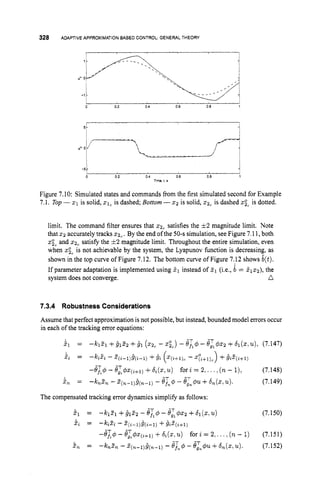
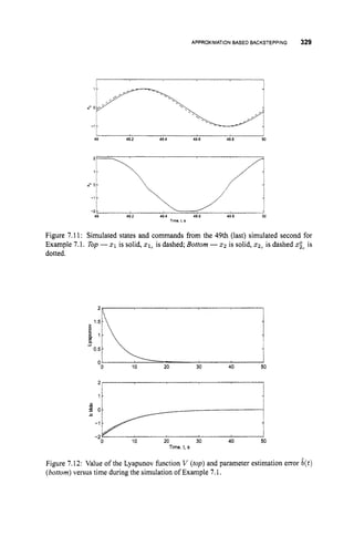
![330 ADAPTIVE APPROXIMATIONBASED CONTROL: GENERAL THEORY
When the projection operators are not in effect, the derivative of the Lyapunov function
reduces to
n
(7.153)
which is negative for CC,kzZT 2 El”=,
2,6,. Therefore, we can prove the following
theorem.
Theorem 7
.
3
.
5 Consider the closed-loop system composed of theplant described in eqns.
(7.13447.132) with the controller of eqns. (7.133)-(7.136) with parameter adaptation
defined by
eft = PB, (rf.#d,(z,6
0
)
) for z = 1,....n (7.154)
g
,
, (7.155)
e,, = psB, (rg,4dn(z,
6 0 ) ~ ) (7.1 56)
= PSB, (rg,&&(a,
60)q2+1)) for = 1,. ..,n - 1
where
where E = $CYZl
6
;
o +,
ufor some ,u > 0 and tc = mini(ki). Assuming that 6i 5 6io
where 60 = [61,, ... ,S,,], this system solves the tracking problem with the following
properties:
1. Zi,2,ef,eg,ef,8, E cm,
2. Ei is small-in-the-mean-square sense, satisfying
3. as t + m, %i i
s ultimately bounded by 5 E.
The proof follows the same lines as those of Theorems 7.2.3and 7.2.5. Therefore, it is left
as an exercise. For hints, see Problem 7.6
7.4 CONCLUDING SUMMARY
This chapter ha5 presented a general theoretical framework for adaptive approximation
based control. The main emphasis has been the derivation of provably stable feedback
algorithms for some general classes of nonlinear systems, where the unknown nonlineari-
ties are represented by adaptive approximation models. Two general classes of nonlinear
systems have been considered: (i) feedback linearizable systems with unknown nonlinear-
ities; (ii) triangular nonlinear systems that allow the use of the backstepping control design
procedure.
Overall, this chapter has followed a similar development as Chapter 5, with the unknown
nonlinearities being replaced by adaptive approximators. In some cases the mathematics
get rather involved, especially when using the backstepping procedure. In this chapter,](https://image.slidesharecdn.com/adaptive-approximation-based-controlcompress-230219164415-f6eb4a64/85/adaptive-approximation-based-control_compress-pdf-348-320.jpg)
![EXERCISES AND DESIGN PROBLEMS 331
as well as in Chapter 6, there was a focus on understanding some of the key underlying
concepts of adaptive approximation.
The development of a general theory for designing and analyzing adaptive approxima-
tion based control systems started in the early 1990s [40, 181,208,211,212,229,232,2731.
In the beginning, most of the techniques dealt with the use of neural networks as approx-
imators of unknown nonlinearities and they considered, in general, the ideal case of no
approximation error. These works generated significant interest in the use of adaptive ap-
proximation methods for feedback control. One direction of research dealt with the design
and analysis of robust adaptive approximation based control schemes [111, 191, 192,209,
2241. There is also considerable research work focused on nonlinearly parameterized ap-
proximators [149, 2161 and output-based adaptive approximation based control schemes
[3,90,112,144]. In addition to the continuous-time framework, several researchers have in-
vestigated the issue of designing and analyzing discrete-time adaptive approximation based
control systems [41, 93, 95, 123, 2101, as well as the multivariable case [94, 1621. Sev-
eral researchers have investigated adaptive fuzzy control schemes and adaptive neuro-fuzzy
control schemes [255,282], as well as wavelet approximation models [25,37, 199,3061. A
significantamount ofresearchwork has focused on adaptive approximation based control of
specific applications, such as robotic systems [92,241,278,275,277]and aircraft systems
[36,77,78]. In addition to feedback control, there has also been a lot of interest in the appli-
cation of adaptive approximation methods to fault diagnosis [50,207,271,276,307,308].
system identification [24, 44, 214, 137, 2281, and adaptive critics [220, 2471. Finally,
it is noted that several books have also appeared in the topics related to this chapter
[15,23,32,63,87,91,101,115,129, 147,148,151,168,189, 197,198,254,264,283,2961.
7.5 EXERCISES AND DESIGN PROBLEMS
Exercise 7.1 Theorem 7.2.3 stability results for a scalar approximation based feedback
linearization approach using a dead-zone. Discuss why violation of the inequality Id1 < 6
,
causes the proof of that theorem to break down. Show that even with the dead-zone, if the
inequality Id1 < b, does not always hold, then the method yields performance similar to
that stated in Theorem 7.2.2.
Exercise 7.2 Complete the stability analysis for the closed-loop systems described in Sec-
tion 7.2.3.
Exercise 7.3 Starting from eqn. (7.64) prove the properties of Theorem 7.3.1.
Exercise 7.4 Complete the stability analysis for the closed-loop systems described in Sec-
tion 7.3.2 with b # 0 (discussed after Theorem 7.3.3).
Exercise 7.5 For the approach derived in Section 7.3.3:
1. derive the dynamic equations for the tracking errors 5, and &;
2. derive eqns. (7.138) and (7.139).
Hint: Use Young’s inequality in the form Z,b, < $Z.f +k6:. Show that
Exercise 7.6 Complete the proof of Theorem 7.3.5.](https://image.slidesharecdn.com/adaptive-approximation-based-controlcompress-230219164415-f6eb4a64/85/adaptive-approximation-based-control_compress-pdf-349-320.jpg)
![332 ADAPTIVEAPPROXIMATIONBASED CONTROL: GENERALTHEORY
Use this expression to show that the time outside the dead-zone is finite. Integrate both
sides of the inequality to derive the mean-squared error bound.
Exercise 7.7 This problem considers the design of u for 2 4 D, for the example of Section
1.2.2.3.
1. For the definition of z on page 302, find the equations for i .
2. Evaluate V for V = i z T z .
3. Show that V 5 -zzh(z2) for the specified u.
4. Discusshowthis factjustifiestheclaimthat initial conditionsoutsideD = [-1.3,1.3]
x
[-1.3,1.3] ultimately converge to V,
but D is not positively invariant. Consider the
initial condition 5 = [1.3,1.3,0].
5. If V were redefined to be V = { ( q r x 2 ) /1 1 ( 2 1 , 5 2 ) / 1 ~
5 1.3}, can you show that
Exercise 7.8 For the detailedexample ofSection 7.2.2.3,design andsimulateda controller
using the backstepping approach discussed in Section 7.3.2.
Exercise 1.9 For the detailed example of Section 7.2.2.3,design andsimulateda controller
using the commandjltered backstepping approach discussed in Section 7.3.3.
the new V is positively invariant.](https://image.slidesharecdn.com/adaptive-approximation-based-controlcompress-230219164415-f6eb4a64/85/adaptive-approximation-based-control_compress-pdf-350-320.jpg)
![CHAPTER 8
ADAPTIVE APPROXIMATION BASED
CONTROL FOR FIXED-WINGAIRCRAFT
Various authors have investigated the applicability of nonlinear control methodologies to
advanced flight vehicles. These methodsoffer both increases in aircraft performance aswell
as reduction of development times by dealing with the complete dynamics of the vehicle
rather than local operating point designs (see Section 5.1.3). Feedback linearization, in its
various forms, is perhaps the most commonly employed nonlinear control method in flight
control [14, 34, 143, 165, 166, 2501. Backstepping-based approaches are discussed for
example in [77,98, 106, 107,2451. Reference [135] presents a nonlinear model predictive
control approach that relies on a Taylor series approximation to the system’s differential
equations. Optimal control techniques are applied to control load-factor in [96]. Prelin-
earization theory and singular perturbation theory are applied for the derivation of inner
and outer loop controllers in [1651. The main drawback to the nonlinear control approaches
mentioned above is that, as model-based control methods, they require accurate knowledge
ofthe plant dynamics. This isof significance in flight control since aerodynamicparameters
always contain some degree of uncertainty. Although, some of these approaches are robust
to small modeling errors, they are not intended to accommodate significant unanticipated
errors that can occur, for example, in the event of failure or battle damage. In such an
event, the aerodynamics can change rapidly and deviate significantly from the model used
for control design. Uninhabited Air Vehicles (UAVs) are particularly susceptible to such
events since there is no pilot onboard. For high performance aircraft and UAVs, improved
control may be achievable if the unknown nonlinearities are approximated adaptively.
Adaptive Approximation Based Control:UnifiingNeural, Fuzzy and TraditionalAdaptive 333
ApproximationApproaches.By Jay A. Farrell and Manos M. Polycarpou
Copyright @ 2006 John Wiley & Sons, Inc.](https://image.slidesharecdn.com/adaptive-approximation-based-controlcompress-230219164415-f6eb4a64/85/adaptive-approximation-based-control_compress-pdf-351-320.jpg)
![334 ADAPTIVE APPROXIMATION BASED CONTROL FOR FIXED-WINGAIRCRAFT
This chapter presents detailed design and analysis of adaptive approximation based
controllers applied to fixed-wing aircraft.' Therefore, we begin the chapter in Section
8.1 with a brief introduction to aircraft dynamics and the industry standard method for
representing the aerodynamic forces and moments that act on the vehicle. The dynamic
model for an aircraft is presented in Subsection 8.1.1. Subsection 8.1.2 introduces the
nondimensional coefficient representation for the aerodynamic forces and moments in the
dynamic model. For ease of reference, tables summarizing aircraft notation are included at
the end of the chapter in Section 8.4.
Two control situations are considered. In Section 8.2, an angular rate controller is de-
signed and analyzed. That controller is applicable in piloted aircraft applicationswhere the
stick motion of the pilot is processed into body-frame angular rate commands. That section
will also discuss issues such as the effect of actuator distribution. In Section 8.3,we develop
a full vehicle controller suitable for UAVs. The controller inputs are commands for climb
rate y, ground track 2, and airspeed V . An adaptive approximation based backstepping
approach is used.
8.1 AIRCRAFT MODEL INTRODUCTION
Since entire books are written on aircraft dynamics and control, this section cannot com-
pletelycoverthetopic. Thegoalofthis section istobrieflyprovide enoughofan introduction
so that readers unfamiliar with aircraft dynamics and control can understand the derivations
that follow.
8.1.1 Aircraft Dynamics
Aircraft dynamics are derived and discussed in e.g. [7, 2581. Various choices are possible
for the definition of the state variables. We will define the state vector using the standard
choice IC = [x,
y,V,p, Q, p;P,Q;R].The subvector [P,
Q:R]is the body-frame angular
rate vector. The components are the roll, pitch, and yaw rates, respectively. The subvector
[p,cy,,3]will be referred to as the wind-axes angle vector. The bank angle of the vehicle is
denoted by p. The angle-of-attack Q and sideslip p define the rotation between the body
and wind frames-of-reference. The variables x and y are the ground-track angle and the
climb angle. Finally, V is the airspeed. For convenience of the reader, the dynamics of this
state vector are summarized here:
1
x = - [Dsinp cosp +Y cosp cos p +L sinp
mV cosy
+T (sincy sinp - cos cy sinp cosp)]
1
i. = -[-Dsinpsinp-Ycos10sinp+Lcosy
mV
+T (sincy cosp +coscy sin @sinp ) ] - -cosy
9
V
1
V = - (Tcoscucosp - Dcosp +Y sin/?) - gsiny
m
= [Dsinptany cosp +Y cosptany cosp +L (tan p +tany sinp) +
mV
'This research was performed in collaborationwith by Barron Associates Inc. and builds on the ideas published
in [77, 781 and the citations therein. The authors gratefully acknowledge the contributions of Manu Sharma and
Nathan Richards to the theoretical developmentand for the implementationof the control algorithm software.](https://image.slidesharecdn.com/adaptive-approximation-based-controlcompress-230219164415-f6eb4a64/85/adaptive-approximation-based-control_compress-pdf-352-320.jpg)
![AIRCRAFT MODEL INTRODUCTION
+T (sina tan y sinp +sina tan p - cos a sin p tan y cos p)]
gtan ,G’cosy cos p
V cos p
-1 g cosy cosp
P,
- +-
& = - [L+Tsina] + +Q-P,tanP
m V c o s p vcos p
1 g cosy sinp
- Rs
V
p = -[Dsinp+Ycosp-Tcosasinp]+
mV
P = ( c ~ R + c ~ P ) Q + c B E + c ~ R
Q = CSPR- c6 (P2- R2)+C,&?
R = (CSP
- c ~ R )
Q +c ~ L
+c ~ N .
In these equations, m is the mass, g denotes gravity, and the ci coefficients for i = 1,...,9
are definedon page 80 in [258]. The variables P, and R, are the stability axes roll and yaw
rates:
cosa sina
[:I=[ -sina c o s a ] [ i]’ (8.10)
The symbols [D,Y,L]denote the drag, side, and lift aerodynamicforces and the symbols
[E,a,I
?
] denote the aerodynamic moments about the body-frame z,g, and z axes, respec-
tively. The aerodynamic forces and moments are functions of the aircraft state and of the
control variables. The control variables are the engine thrust T and the angular deflection
of each of the control surfaces denoted by the vector 6 = [Sl,...,
6
,
]
. The control signal
6does not appear explicitly in the above equations, but may affect the magnitude and sign
of the aerodynamic forces and moments. See Section 8.1.2 for further discussion.
Tables 8.2, 8.3, and 8.4 at the end of this chapter define the constants, variable, and
functions used in the above equations. For the discussion to follow, we will assume the
(nominal) aircraft is tailless and configured with p = 6 control surfaces.
8.1.2 NondimensionalCoefficients
In the aircraft literature, these aerodynamic force and moments functions are represented
by nondimensional coefficient functions. In this approach, the basic structure of the model
and the major effects of speed, air density, etc. are accounted for explicitly for a general
class of air vehicles. Nondimensional coefficient functions relate the general model to a
specific vehicle in the class.
For example, the aerodynamic forces might be represented as
m
(8.1 1)
/ m
(8.13)
where Q = is the aerodynamic pressure, S is the wing reference area, b is the reference
wing span, and p is the air density. The subscripted ‘C’ symbols are the nondimensional](https://image.slidesharecdn.com/adaptive-approximation-based-controlcompress-230219164415-f6eb4a64/85/adaptive-approximation-based-control_compress-pdf-353-320.jpg)
![ANGULAR RATECONTROL FOR PILOTED VEHICLES 337
1 0
[z]= [ 0 I ] [ : : ]
The transfer function from P,P to P, is given by
(8.14)
which has unity gain at low frequencies, damping specified by C,and undamped natural
frequency equal to w,. As long as wnis selected to be large relative to the bandwidth of
P,"(t),the error P,"(t)- Pc(t)will be small. Also, by the design of the filter, the output
Pc(t)is the integral of the output P,(t).In the analysis of the control law,we will prove that
P(t)converges to and tracks Pc(t).Therefore, the response of P(t)to the pilot command
P," (t)is determined by this prefilter; therefore, the prefilter determines the aircraft handling
qualities. Similar prefilters are designed for Q
Z and R,".
8.2.1 Model Representation
The angular rate dynamics of eqns. (8.7H8.9)
can be written as
i = A(fo +f*)+F ( x )+B(Go+G*)6 (8.15)
where z = [P,Q,RIT and A = B = are known matrices. The inertial
terms represented by
1
(ciR+c2P)Q
c ~ P R
- (P2- R2)
(c6p- CZR)
Q
are assumed to be known. The aerodynamic moments are represented as
L'
(fo +f*)= [:
: ] and (Go+G*) =
In this representation, fo and G
o represent the baseline or design model, while f' and G*
represent model error. The model error may represent error between the actual dynamics
and the baseline model or model error due to in-flight events.
The control signal will be implemented through the surface deflection vector 6 =
[&....,&IT. The objective of the control design is to select 6 to force [P(t),
Q(t),
R(t)]
to track [P,(t),
Qc(t),
R,(t)]in the presence of the nonlinear model errors f *and G*.
8.2.2 Baseline Controller
This subsection considers the design of an angular rate controller based on the design model
without function approximation. The objective is to analyze the affect of model error and
to illustrate that the approximation based controller can be considered as a straightforward
addition to the baseline controller that enhances stability and performance in the presence
of errors between the baseline model and the actual aircraft dynamics.](https://image.slidesharecdn.com/adaptive-approximation-based-controlcompress-230219164415-f6eb4a64/85/adaptive-approximation-based-control_compress-pdf-355-320.jpg)
![338 ADAPTIVEAPPROXIMATION
BASED CONTROLFOR FIXED-WING
AIRCRAFT
Since the functions f *and G" are unknown, the baseline controller design is developed
using the following design model.
i = Afo +F ( z )+BGo6.
Therefore, we select a continuous signal 6 such that
BGo6 = -Afo - F - KE +ic; (8.16)
where K isapositivedefinitematrix, E = z-z,, zc = [Pc,
Qc, &ITandi, = [pc,
Qc,&,IT.
Since the aircraft is over-actuated (i.e., Go E T-?3x6), the matrix BGo will have more
columns than rows and will have full row rank. Therefore, many solutions to eqn. (8.16)
exist. Some form of actuator distribution [26,68,701 is required to select a specific 6. For
example, the surface deflections could be defined according to
6= d +W-lG;BT [BGoW-'G:BT]-' (u,- BGo d ) , (8.17)
where W is a positive definite matrix, d E !R6is a possibly time-varying vector, and uc =
-Afo -F -KE +iC.
This actuator distribution approach minimizes (6 - d)T W (6 - d)
subject to the constraint that uc = BGo6. It is straightforward to simply let d be the zero
vector; however, it is also possible to define d to decrease the magnitude and rate of change
of 6.
Whena surface deflection vector 6 satisfyingeqn. (8.16) is appliedto the actual dynamics
of eqn. (8.15), the resulting closed-loop tracking error dynamics reduce as follows:
i =
=
Afo +F ( z )+BGo6 +Af* +BG'6
-KE +i,+Af* +BG*6
5 = -KE+Af* +BG*6. (8.18)
If the design model were perfect (i.e., f* = 0 and G* = 0), then we would analyze the
Lyapunov function V = $ZT.Z. The time derivative of V along solutions of eqn. (8.18)
with f* = 0 and G* = 0 is V = -ETKE which is negative definite. Therefore, relative
to the design model, the closed-loop system is exponentially stable (by item 5 of Theorem
A.2.1).
Relative to the actual aircraft dynamics, the derivative of the Lyapunov function is V =
-ETKE +5T (Af' t BG'6). Nothing can be said about the definiteness properties of
this time derivative without further assumptions about the modeling errors f* and G*. If
f *and G*satisfycertain growth conditions (e.g., see the topic of "vanishing perturbations"
in [134]), then the system is still locally exponentially stable. Note that such vanishing
perturbation conditions are difficult to apply in tracking applications. As the modeling
errors f* and G' increase, the closed-loop system may have bounded tracking errors or be
unstable. However, nothing specific can be said without more explicit knowledge of the
model error.
8.2.3 Approximation Based Controller
The approximation based controller will select a continuous signal 6 such that
B ( G ~
+G) 6= - A ( j o+f) - F - K Z+i,, (8.19)](https://image.slidesharecdn.com/adaptive-approximation-based-controlcompress-230219164415-f6eb4a64/85/adaptive-approximation-based-control_compress-pdf-356-320.jpg)
![340 ADAPTIVE APPROXIMATION BASED CONTROL FOR FIXED-WING AIRCRAFT
The functions f* and G* are defined similarly as
b
P
b O O (CEO + C E P Z +CLOP)
4)
O O b ( c N o + c N p 2 V + C N , ~ + C -
bP
(CM, +CM, $8)
(8.22)
(8.23)
The unknown portion of each nondimensional coefficient function will be approximated
during aircraft operation. The coefficient c~ will be approximated as EL" (alM ) =
e & # ~ , ( a ~
M ) where 4 ~ ~ ( a ~ M )
: !R2 c-t !Rfiis a regressor vector that is selected by
the designer. The coefficient csP will be approximated as EN^ (a.M ) = O ~ . p # ~ p
(a.M ) .
The approximations to the other 28 coefficient functions are defined similarly. While it
is reasonable to use different regressor vectors such as # f i p (a,Ad) for each coefficient
functions, in this case study we uses a single regressor vector for all the approximated co-
efficient functions for notational simplicity: #(a.M ) = $ L ~
= $ f l P = .... The regressor
vector d(a,M ) will be defined sothat it is a partition of unity for every (a,M ) E V where
D = DoXVM
iscompactwithD, = [-7,151 degreesandDM = [0.2,1.0]. Thevariables
a and M are outside the control loop, but are affected by the angular rates. It is assumed
that the pilot issues commands (P,"l
QZ.I?:) and controls the engine thrust to ensure that
(a,M ) remains in 2
)
.
An alternative way of stating the ideas at the end of the previous paragraph is that the
aircraft designers specify an operating envelope V = Va x VM.The control designers
develop a controller with guaranteed performance over V.The pilot must ensure that the
angular rate and thrust commands maintain (a(t).
M(t))E D for all t.
The functions fand G can be reconstructed from the approximated coefficient functions
(8.25)
where the arguments to the functions have been dropped to simplify the notation. For
the analysis that follows, it is useful to note that f can be manipulated into the standard
Linear-In-the-Parameter (LIP) form f = @:Of where
1
and
EL6, EL,, ... EL,,
EM,, EGa2 , . . EM,- ,
en,, EN6, ... ENarn
@ T - T
- [eE0,
... OX,]E %IoN](https://image.slidesharecdn.com/adaptive-approximation-based-controlcompress-230219164415-f6eb4a64/85/adaptive-approximation-based-control_compress-pdf-358-320.jpg)
![ANGULAR RATE CONTROL FOR PILOTED VEHICLES 341
and @f E !R10Nx3. This representation is not computationally efficient, since @pf is sparse,
but simplifies the qotation of the analysis. Similarly, the j-th column of the matrix G can
be represented as G, = @
;
, QG, where
@, = ] E ! R ~ ~ ~ ~
and @G, E !R3Nx3 forj = 1.... ,6.
3.1.3, we know that there exists optimal 0; and @&, such that
Finally, over a compact region V,
which represents the operating envelope, from Section
j * = @T@;+ef (8.26)
Gj = @ & 3 0 & 3 + e G 3 f o r j = l , ...,m (8.27)
where ef and eG, are bounded with the bound determined by V and the choice of 4. The
approximation parameter errors are defined as
Of = of-@; (8.28)
6 G 3 = oG, - for 3 = 1,.
..,m. (8.29)
With the approximator defined as in this subsection, the tracking error dynamics of eqn.
(8.20) reduce to
8.2.3.2 ParameterAdaptation. We select the parameter adaptation laws as
Gf =bf z Pf (rf@fATZ) (8.31)
6 G l = b G , = PG, (rG,@G,BTZ6j) , (8.32)
where rf and r G , are positive definite matrices. The signal
2 ifX&l)z > &
f = { 0 otherwise
where XK is the minimum eigenvalue of K. This adaptation law includes dead-zone and
projection operators. The projection operator Pf ensures that each element of 0, remains
within known upper and lower bounds: eft5 Ofb5 Qf,. Therefore, the Pf projection
operator acts componentwise according to
7%
0 otherwise
where 7 = rf@fATZ. The projection operators PG, for j = 1,...,m must maintain
boundedness of the elements of OC, and full row rank of the matrix G. The row rank of G
is determined by the row rank of the matrix
ifOf, I Of,
IQfz
Pf,(TZ) = {
c;*,
+ELS, L*2 +E& ... Ct,, +EL.*,
C&&,
+E$f&l co-
M82 +EM&, ... C
&
, +E$I.,,
Cg6,+E.V&, c*;*,
+ENs2 ... C5&, +E.v&m](https://image.slidesharecdn.com/adaptive-approximation-based-controlcompress-230219164415-f6eb4a64/85/adaptive-approximation-based-control_compress-pdf-359-320.jpg)
![ANGULAR RATE CONTROL FOR PILOTED VEHICLES 345
the parameters that result in a locally accurate fit to the functions f* and G*. This would
be an example of the approach adapting the parameters to the local situation when it is
not capable of learning the parameters that would be globally satisfactory over V.A very
simple example illustrating this issue is described in Exercise 8.1.
8.2.4 SimulationResults
Thissection presents simulation results fromthecontrol algorithms developed inthis section
when applied to the Baron Associates Nonlinear Tailless Aircraft Model (BANTAM),
which is a nonlinear 6-DOF model of a flying-wing aircraft. BANTAM was developed
primarily using the technical memorandum [80], which contains aerodynamic data from
wind-tunnel testing of several flying-wing planforms, but also using analytical estimates
of dynamic stability derivatives from DATCOM and HASC-95. The flying wing airframe
is particularly challenging to control as it is statically unstable at low angles-of-attack
and possesses a restricted set of control effectors that provide less yaw authority than the
traditional set used on tailed aircraft. The control surfaces consist of two pairs of body
flaps mounted on the trailing edge of the wing. Additionally, a pair of spoilers are mounted
upstream of the flaps. This configuration generally relies upon the flaps for pitch and roll
authority and the spoilers for yaw and drag. The simulation model also contains realistic
actuator models for the control effectors with second order dynamics and both position and
rate limits. The body flap actuators have 40 radsec bandwidth with 3=30deg position limits
and 590 deghec rate limits. The spoiler actuators are identical except that they can only
be deflected upwards and their motion is limited to 60 deg.
Simulation results are shown in Figures 8.1-8.3. The simulation time is 100 s, with a
simulated pilot generating the signals (P,".
Q:, Rz). Each (Pi:Q:, R:)-command filter
is of the form of eqn. (8.14). Each uses a damping factor of 1.O and undamped natural
frequencies of 20,20, and 10 *,respectively.
At t = 0, the known portion of the model described in (8.21H8.22) is defined using
constant values for each of the nondimensional coefficient functions C,O. The constant
values were selected so that the coefficient functions were approximately accurate near
a = 0" and M = 0.46. The approximated functions f and G were initialized to be zero by
defining each approximated coefficient function 2, in (8.24)<8.25) to be zero. The control
law is specified by (8.19). The control gain matrix is K = diag(20.20,lO).Parameter
adaptation is specified by (8.31H8.32) with the dead-zone defined by E = 1,which implies
that parameter adaptation will stop if 112112 < f = 0.19.
As the simulation progresses,
the tracking of the (filtered) pilot specified command trajectory should improve as the
functions f^and G are increasingly well-approximated.
During the first 5 s of the simulation, the P,"
and R: signals are zero. The pilot adjusts
the Q: signal to attain stable flight near the initial flight condition with an airspeed of
500 fps, altitude of 4940 ft, and angle-of-attack of 3.6'. For t 6 [5,50]s,the pilot issues
(P,".Q:, R:) to perform aircraft maneuvering along a nominal trajectory. At t = 50s, the
right midflap fails to the zero position. Throughout the simulation, the approximated model
must be adjusted to maintain stability of the closed-loop and to attain the desired level of
tracking performance.
The simulation was ran twice, once with learning off and once with learning on. The
learning off simulation corresponds to the baseline controller. Other than turning learning
on or off, all parameters were identical for the two simulations. The results in the left
column of each figure correspond to the simulation with learning off. The results in the
right column of each figure correspond to the simulation with learning off.
-K](https://image.slidesharecdn.com/adaptive-approximation-based-controlcompress-230219164415-f6eb4a64/85/adaptive-approximation-based-control_compress-pdf-363-320.jpg)
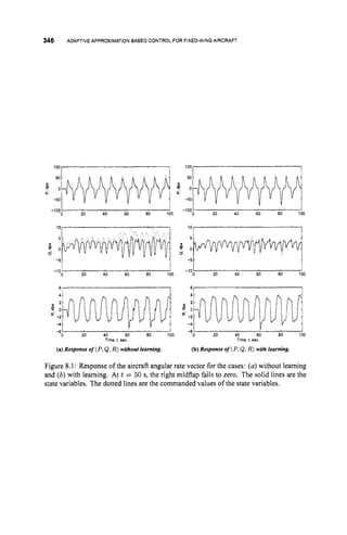
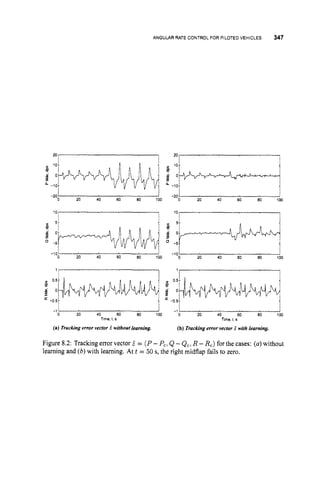
![348 ADAPTIVE APPROXIMATIONBASEDCONTROL FOR FIXED-WING AIRCRAFT
Figure 8.1 plots the variables (P,Q.R)as a solid line and (P,, Q,, R,) as dashed lines.
The units are degrees per second. Note that the pilot serves as an outer loop controller who
adjusts the commands to maintain the nominal vehicle trajectory based on the response of
the aircraft. Therefore, the nominal commands (P,",QZ,
RZ)with and without learning are
slightly different. Without the feedback action of the pilot, the trajectory tracking errors
would accumulate resulting in the aircraft in the two simulations ultimately following very
distinct trajectories. With the pilot feedback the operating point maintains M E [0.44,
.47]
throughout both simulations; and maintains cy E [1.8,5.1]
deg. throughout the simulation
with learning and cy E [0.6,5.1]deg. throughout the simulation without learning.
Due to the scale of Figure 8.1, the differences in tracking error between the two simula-
tions are not easily observed; therefore, Figure 8.2 directly plots the tracking error vector
2 = ( P - P,, Q - Q,, R - R,). The P and Q variables show clear improvements as a
result of the adaptive function approximation. Note that, in the case that learning is used, as
experience is accumulated, first fort E [0,50]s
and then fort E [50,100],
the tracking error
decreases toward the point where it will be within the adaptation dead-zone. The change
in performance in the R variable is minor for a few reasons. First, the control authority for
the R state is limited. Second, the rate of learning is related to the size of the tracking error.
Since the magnitude of the R tracking errors are initially small, so are the changes to the
functions affecting R.
-5 -5
-10 -10
30 40 50 60 70 30 40 50 60 70
10, , 101 1
I
50 60 70
40
-15'
30
4
-right
p 3 left
(a) Commanded surface deflections without learning.
-10 right
-1530 40 50 60 70
-
left
1 -
30 40 60 70
50
0
(b) Commanded surface deflections with learning.
Figure 8.3: Commanded surfacedeflections fort E [30,70]
s. At t = 50 s,the right midflap
fails to zero instead of tracking the command shown in this figure.
Figure 8.3 displays a portion of the time series of the surface position commands. Only
a portion of the time series is shown sothat the time axis can be expanded to a degree which
allows the reader to clearly observe the signals. The selected time period includes 20 s](https://image.slidesharecdn.com/adaptive-approximation-based-controlcompress-230219164415-f6eb4a64/85/adaptive-approximation-based-control_compress-pdf-366-320.jpg)
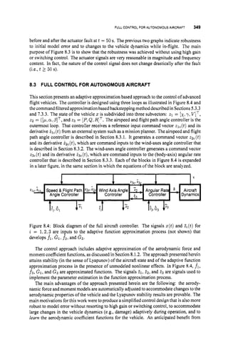
![350 ADAPTIVE APPROXIMATION BASEDCONTROLFOR FIXED-WING AIRCRAFT
these properties is that the controller could be applied to an aircraft for which it was not
explicitly designed, e.g., an aircraft of the same family but different configuration. Addi-
tionally, the controller could be developed using a lower fidelity model than required by
current methods, thereby offering a cost savings. Thiscontrolmethod is expected to provide
significant reduction in design time since the control system design does not depend on a
conglomeration of point designs.
The functions that are approximated adaptively will use a basis set defined as a function
of angle-of-attack a and Mach M . Successful implementation of the approach assumes
that we can define a set V, = [a-.6
1 with < 0 < d and L(Q- E,) < 0 < L(6 +E,)
where L(x)denotes the lift force evaluated at 5 , and E, > 0 is a designer-specified small
constant. The approximated functions will be designed assuming that A4 E [0.2.1.0]and
a E V$ = [a-- E,. 6 +E,]. We assume that the region V$has been defined so that stall
will not occur for a E Vo,'.
Finally, we assume that a(0)E Vo,'
and that crc(t)E V,for all
t 1 0, where a, is an angle-of-attack command defined following eqn. (8.41)in Section
8.3.1.
Most of the assumptions stated in the previous paragraph are, in fact, operating en-
velope design constraints that the planner can enforce by monitoring and altering the
z
l
, = [xl,,yl,. VlClTcommands that it issues. For example, as the control signal ac(t)
approaches d from below, the planner can decrease ylc, decrease the magnitude of xl,,
or increase VlC. Determining the combination of these options most appropriate for the
current circumstance of the aircraft is straightforward within a planning framework. Given
the above conditions, analysis showing that a(t)E '
D
:
, Vt > 0 is presented in Subsection
8.3.2.3.
Each of the next three subsections derives and analyzes the control law for one of the
three control loops depicted in Figure 8.4. Since that presentation approach leaves the
control algorithm interspersed with the analysis equations, the control law and its stability
properties are summarized in Section 8.3.4.The structure of the adaptive approximators
are defined in Section 8.3.5.Section 8.3.6contains a simulation example and discussion of
the controller properties.
8.3.1 Airspeed and Flight Path Angle Control
Let the state vector 21 be defined by z1 = [x,
y, VIT. To initiate the command-filtered
backstepping process, we need a control law that stabilizes the 21 dynamics in the presence
ofnonlinear model error. We assume that the command signal vector 21, = (xc,
"ic,V,) and
its derivative 21, is available, bounded, and continuous. The airspeed V will be controlled
via thrust T. The flight path angles (x,
y) will be controlled through the wind-axes angles
( p ,a);therefore, p l = [p,a,TITis the control signal for zl.
The block diagram of the
controller derived in this subsection is shown in Figure 8.5.
The airspeed and flight path angle dynamics of eqns. (8.1)-(8.3) can be represented as
.ii =Aifi +Fi +Gi(Pirx)
cosp cos p/ cosy
cosp sin p
sin p cosp/ cosy
- sin/?sin p
-
- v c o s p V sin/?
with Al =
(Tcoscusinpsinp - mgcosy)
-T cos a sin p cos p h
F I = [-g siny
,p1 =
1
(8.35)](https://image.slidesharecdn.com/adaptive-approximation-based-controlcompress-230219164415-f6eb4a64/85/adaptive-approximation-based-control_compress-pdf-368-320.jpg)
![FULL CONTROL FOR AUTONOMOUS AIRCRAFT 351
. A A
Zlc Command
Calculation Filter
7
l
h
l z2c
Figure 8.5: Block diagram of the airspeed and flight path angle controller described in
Section8.3.1. Thesignal zl(t)isasubvectorofz(t).The functions f1 anddl areoutputsof
the adaptive function approximation process (not shown). The nominal control calculation
refers to the solution of eqn. (8.39). The signals z1, and il, are inputs from the mission
planner. The signals t2, and i2,are outputs to the wind-axes angle controller described
in Section 8.3.2. The signal Z1 is a training signal output to the function approximation
process.
and
:
:]=
uv
3 (8.36)
where
PI^,z) = (J%L~~.
x)+TsinPlz1 (8.37)
UP12 1 .
) = Lo(z)+LY(X)Plz. (8.38)
The drag, lift, and side force functions that are used in the definitions of f1, L,(z), and
L,(x) are unknown. The function Fl is known.
We select the control signal PI,with K1positive definite, so that the following equation
is satisfied
Gl(p1?X) = -K1il +i?iC
- Al.fi - F
1 (8.39)
where f1 = [b(z),
Y ( x ) .
-k(z)lTand
L m
(8.40)](https://image.slidesharecdn.com/adaptive-approximation-based-controlcompress-230219164415-f6eb4a64/85/adaptive-approximation-based-control_compress-pdf-369-320.jpg)
![352 ADAPTIVEAPPROXIMATION
BASED CONTROLFOR FIXED-WING
AIRCRAFT
withg(pI2,z)= & ~ l ~ , z ) + T s i n p 1 , .The functions [B(z),
Y ( z ) ,
i(z)]areapproxima-
tions to [D(z),
Y ( z ) ,
L(z)].
The effect of the error between these functions is considered
in the analysis of Section 8.3.2.1. The solution of eqn. (8.39) for 1-11 is discussed in Section
8.3.1.1.
Assuming that the solution p1 to (8.39) has been found, let z;, = [p:.a,",
&'IT. To
produce the signals z2, and &, which are the command inputs to the wind-axes angle
controller, we pass zi, through a command filter. The error between t
i
,and 22, will be
explicitly accounted for in the subsequent stability analysis. Define 21 = 21 - [I where
the variable (1 is the output of the filter
61 = -Kit1 + (GI(,,, z) - G ~ ( Z ; ~ ,
z)) . (8.41)
The purpose of the command filter is to compute the command signal 22, and its deriva-
tive i2,, This is accomplished without differentiation. The purpose of the &-filter is to
compensate the tracking error 21 for the effect of any differences between 22 and .ti,.In
the analysis to follow, we will prove that dl is a bounded function. By the design of the
command filter, the difference between z2, and z;c will be small. Finally, in the following
subsections, we will design tracking controllers to ensure that the difference between 22
and z2, is small. Therefore, (1 will be bounded, because it is the output of a stable linear
filter with a bounded input.
8.3.1.1 Selection of a and p Commands. The value of the vector pl in the left-
hand side of eqn. (8.39) must be derived, as it determines the command input to the
wind-axes angle loop. Because all quantities in the right-hand side of eqn. (8.39) are
known, the desired value of GI(p1,z) can be computed at any time instant. The purpose
of this subsection is to discuss the solution of eqn. (8.40) for 1-11. Note that = 1-1:
and p l z = a,"are the roll-angle and angle-of-attack commands. Also, to decrease the
complexity of the notation, we will use the notation g(a,")
instead ofg(,u12,
z). Finally, for
complete specification of the desired wind-axes state, we will always specify p," as zero.
Defining (X,Y )such that the first two rows of eqn. (8.40) can be written as
we can interpret (X,Y )= (cos(y)mVC,. mVB,) as the known rectangular coordinates
for a point with (signed) radius fj(a:)and angle p: relative to the positive Y axis. Since the
force g(@) may be either positive or negative, there are always two possible solutions, as
depicted in Figures 8.6a and 8.6b. Switching between the two possible solutions requires
p: to change by 180 degrees as g(a,")
reverses its sign. When g(@) reverses its sign, the
point (X,Y )passes through the origin. If g(az)is selected to be positive for a sufficiently
aggressive diving turn (i.e., xc and $c both large), then the maneuver would be performed
with the aircraft inverted (i.e., roll greater than 90 deg). When choosing (&, a:) to satisfy
eqn. (8.40), the designer should only allow i(a:)to reverse its sign when ti, is near zero.
If the sign of g ( a ) reversed while ti, was non-zero, then 1-1: would also need to change so
that (sin(&?),cos(p,"))would have the correct signs to attain the desired control signals.
This change is a 180' roll reversal.
Once p: and a: have been specified, the third equation of eqn. (8.40) can be directly
solved for T.](https://image.slidesharecdn.com/adaptive-approximation-based-controlcompress-230219164415-f6eb4a64/85/adaptive-approximation-based-control_compress-pdf-370-320.jpg)
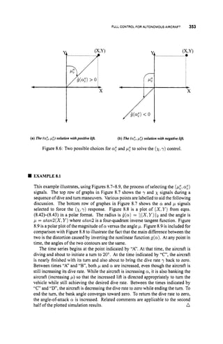
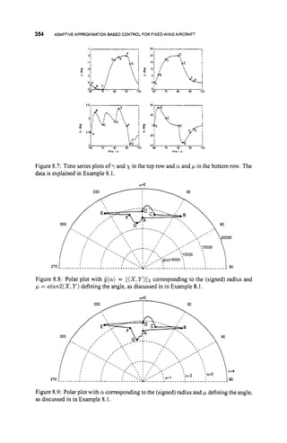
![FULLCONTROL FOR AUTONOMOUS AIRCRAFT 355
Figure 8.10: Block diagram of the wind-axes controller described in Section 8.3.2. The
signal zz(t) is a subvector of z(t).The function f l is an output of the adaptive function
approximation process (not shown). The nominal control calculation refers to the solution
of eqn. (8.44). The signals 2 2 , and i2, are inputs from the flight path angle controller of
Section 8.3.1. The signals 23, and 23, are outputs to the angular rate controller described
in Section 8.3.3. The signal <3 is an input from the angular rate controller. The signal 22 is
a training signal output to the function approximation process.
8.3.2 Wind-Axes Angle Control
Let 21 be as defined in Section 8.3.1. Define 22 = [p,a;PIT. Then, the combined ( z 1 ~
2 2 )
dynamics are
& = Ai(z)fi +Fi(2)+Gi(22,x:T)
i 2 = Az(2)fi +Fz(z)+B2pz
O % l
COS 0
where Bz = [ - c o Z a n p 1 -sinatan0
1 sin0 o -cosa J
1
sin /3 cosp tan y cosp cosp tan y
sin D cos p 0
(tan p +tan y sin p )
A2 = - 0 -1/cosp
mV
mV
l [
1
(sina:tan y sin p +sin a:tan - coy a:tan y cospsinp) T - mgcosycosp tanp
[-T sin (Y +mg cosy cosfi] 5
-7 sin p cos a + mg cosy sin p
l [ O
Fz = -
are known functions and p2 = [P,QIRIT. Note that the ( q ,
22) dynamics are not trian-
gular, since Al, f1, F1 all depend on z2. Nevertheless, the command filtered backstepping
approach is applicable. The block diagram of the controller derived in this subsection is
shown in Figure 8.10.
Select pzc such that
B2pgc = -K252 +22c - Azfi - F2 +qa (8.44)](https://image.slidesharecdn.com/adaptive-approximation-based-controlcompress-230219164415-f6eb4a64/85/adaptive-approximation-based-control_compress-pdf-373-320.jpg)
![356 ADAPTIVE
APPROXIMATION
BASED CONTROLFOR FIXED-WING
AIRCRAFT
with K 2 positive definite and diagonal. The function qa will be defined in Subsection
8.3.2.3 to ensure that cy remains in 2
7
:
. When cy E VQ,
qQwill be zero. Eqn. (8.44) is
always solvable for pzc since B 2 is well defined and nonsingular (for p # +goo).
To specify the angular rate control command signal tg,, we define
& = Pic - t3. (8.45)
where [
3 will be defined in Section 8.3.3. The signal 230, is input to a command filter with
outputs 23, and is,. The variable & is the output of the filter
(2 = - K 2 t 2 +B 2 (23, - 230,) (8.46)
and the compensated tracking error is defined as 22 = 52 - (2. The command filter is
designed to ensurethat 1B22 ( ~ 3 ~
- 230,) I 5 +cQ where K 2 2 denotes the second diagonal
element of K 2 and B 2 2 is the second row of B 2 . This is always possible, since the matrix
B 2 is bounded (since ,
!
?is near zero). Therefore,
(8.47)
E a
2
It221 I -
where (22 is the second element of (2. This bound is used later in the analysis.
8.3.2.1
vious section, for cy E 272,the dynamics of the z1 and 22 tracking errors can be derived:
Tracking Error Dynamics for Q E 232. Given the definitions of the pre-
i, = Alfl +Fl +Gl(Plrz) - 2lc
+( G ~ ( ~ Z ~ Z )
- G : 1 ( . ~ 2 , 2 ) )
+( G i ( ~ 2 , z )
- Gi(p1.z))
= -Ki% - Aifi + (Gi(z21.) - G i ( 2 2 , z ) ) +( G i ( 2 2 . 5 ) - G i ( ~ i , z ) )
= -KiEi - Aifi +( G i ( z 2 . 5 ) - G i ( p 1 , ~ ) ) . (8.48)
fl(z)- fl(z)and algebraic manipulations result in Alfl = A1f1 -
A1 = - [ ---SyWl cospsinp cosp ]. (8.49)
where fl(z)
( G l ( z 2 . z ) - G 1 ( ~ 2 , z ) ) with
sin @cosp/ cosy cosP cos pl cosy
V sin(@) 0
mV
Similarly, the tracking error dynamics for z2 are
42 =
=
A2f1 +F2(2)+B2~30,-i 2 , +B 2 (z3 - 23,) +B 2 (2& - 230,)
A 2 f i +F2(.) +B 2 & -B 2 6 3 - i2, +B 2 (23 - ~ 3 , )
+5’2 (23, - 230,)
-K252 +B223 - A2f1 +B 2 (QC - z&) +qQ.
= -K2& +B 2 f 3 - B2(3 - A2f1 +B 2 (23, - ~ 3 0 ~ )
+TQ
= (8.50)
Combining eqns. (8.41) and (8.46), respectively, with eqns. (8.48) and (8.50), the
dynamics of the compensated tracking errors are
-z’1 = (-K151 - A l f l +( G l ( 2 2 , Z ) - G,(p1,5,,)
- (-K1&+ ( G l ( Z 2 , Z ) - Gl(z;~.z)))
= -K12l -Alf, (8.51)
i 2 = (-K252 +&% - A 2 j 1 +B2 (2gC - z.&) +lla>- (-K2& +B 2 (z3, - 230,))
= - K 2 & - A2f1 +B 2 2 3 +77,. (8.52)](https://image.slidesharecdn.com/adaptive-approximation-based-controlcompress-230219164415-f6eb4a64/85/adaptive-approximation-based-control_compress-pdf-374-320.jpg)
![358 ADAPTIVE APPROXIMATIONBASED CONTROL FOR FIXED-WING AIRCRAFT
The portion of the control law denoted by qa is responsible for ensuring that a remains
in the region of approximation Vifor all t 2 0. We choose q,(a) = [0, -s,(a), 0lT
where
r,(a- (cy- 3))i f a 5 cy- %
s,(a)= w ( a - ( d + % ) ) i f a > f i + %
{: 0 otherwise
as illustrated in Figure 8.11, The magnitude constraint on M > 0 is discussed below in
(8.58). With this definition of ?,(a) and (8.50) the a dynamics are
where K22 denotes the second diagonal element of K2 and B22 is the second row of B2.
Also, note that a&> 0 for a E V
: -Va.
Consider the time derivative of the function V, = $a2:
On the set a E 2
3
: - V,,the term -aK226 5 0 which yields
We will select M to satisfy
The last three terms in this constraint can be directly computed. The first term -
must be upper bounded.
Note that the definition of s
, ensures that the quantity --(Ls(Q) is negative for a E
(d +9,d +E,] and a E [cy-~ ~ , c y
- 3).
Constraint (8.58) ensures that
for a E (6+ SE,, d + and a E [a- E,,Q - SE,). Note that a exiting V
: would
require V, to be positive for either a E (6+ d +E,] or a E [g
-E,, a- ice). Since
we havejust shown V, to be negative on each of these regions, a cannot exit V
: (i.e., 2
3
:
is positively invariant).
Finally, as discussed following (8.57), ifwe can show that the quantity Zzq, = -(a -
&)s, (a)is always non-positive, then itcanbe dropped in the subsequent analysis of(8.57).
We need to consider three cases:
Fora E [cy--~,.g-?f],thefactors,(o) 5 Owhile(ti-E,) 5 Obecauseti 5 -%
For a E [cy- y .d +41,the term Z ~ Q ,= 0.
while ltal5 3;
therefore, Zlv, 5 0.](https://image.slidesharecdn.com/adaptive-approximation-based-controlcompress-230219164415-f6eb4a64/85/adaptive-approximation-based-control_compress-pdf-376-320.jpg)
![FULL CONTROL FOR AUTONOMOUS AIRCRAFT 359
Figure 8.11: Nonlinearity used in the computation of vaas described in Subsection 8.3.2.3.
Note that this figure greatly exaggerates the size of
For a E [G +5f ~ d +4,the factor sa(a)1 0while (6-&) 2 0because d 2 4
The inequalities on d are derived using the assumed range of a and the fact that a,(t) E Da
for all t 2 0. The inequality on is given by (8.47).
while ita[
5 %;therefore, ,i?zqa5 0.
8.3.3 Body Axis Angular Rate Control
Given the results of the previous sections, the objective of this subsection is to design a
tracking controller to force 23 to track 23, while ensuring the stability of the overall system.
This controller and its derivation are very similar to that of Section 8.2. A block diagram
representation of the controller derived in this section is shown in Figure 8.12.
The aircraft dynamics of eqns. (8.1)--(8.9) can be written as
i i = Ai(z)fi + F i ( z ) + G i ( z z , z , T )
i 2 = Az(z)fi+Fz(z)+B 2 ( 2 ) ~ 3
4 = A3f3 +F3(5)+B3G36
where 6 = [dl, .. ..&ITis the control signal, B3 = A3 = [
matrices, F3 =
i]are known
1
[
[;
; . . ' E 6 6 ]
(ciR+czp)Q
c5PR - Cg (P'- R2)
(CsP-czR)Q
is aknown function, and f 3 = [z',
A
?
. n']
... R&
and G3 = A?,jl . a A?&6 are unknown functions. The notation for the moment
functions was defined in Section 8.1.2.
Select continuous 6,"
such that
B3G3b,O= -A3f3 - F3 - K3i3 +23, - B,TZ2, (8.59)
with K3 positive definite. When the aircraft is over-actuated, the matrix B3G.3 will have
more columns than rows and will have full row rank. Therefore, many solutions to eqn.
(8.59) exist and some form of actuator distribution [26,68,70] is required to select 6,"
(see
Section 8.2.2).](https://image.slidesharecdn.com/adaptive-approximation-based-controlcompress-230219164415-f6eb4a64/85/adaptive-approximation-based-control_compress-pdf-377-320.jpg)
![360 ADAPTIVEAPPROXIMATION
BASED CONTROLFOR FIXED-WING
AIRCRAFT
Figure 8.12: Block diagram of the angular rate controller described in Section 8.3.3. The
signal z3(t) is a subvector of z(t).The functions f3 and G 3 are outputs of the adaptive
function approximation process (not shown). The nominal control calculation refers to
the solution of eqn. (8.59). The signals 23, and .i3, are inputs from the wind-axes angle
controller of Section 8.3.2. The signal (3 is an output to the wind-axes angle controller.
The signals 6,is the surface deflection command. The signal 23 is an output training signal
to be used by the adaptive function approximation process.
We pass 6
; through a filter, to produce 6 which is within the bandwidth limitations of
the actuation system.2 The signal (3 is the output of the filter
63 = -K3(3 +B3G3 (
6- 6,") (8.60)
and the compensated tracing error is defined by 23 = 23 - (3.
Finally, select the moment function parameter adaptation laws as
(8.61)
with E = [&I,E Z . &3lT being a vector of designer-specified constants, d3 is the j-th element
of 6, rf3and rG3] being positive definite matrices of appropriate dimensions, and the
function 'T defined in (8.66). The parameterization of .f3 = @T3@f3and G 3 ] = @&,, @ G ~ ~
is derived in Section 8.3.5.
8.3.3.I TrackingError Dynamics and Stability Analysis The tracking error and
compensated tracking error dynamics for z1 are given by eqns. (8.48) and (8.53). The
ZAlternatively,if the surface deflection is measured, then the signal 6
; could be used as the commanded surface
positionsand the measured surface deflectionvector 6can be used directly to calculate E3. No change is required
in the notation of eqn. (8.60).](https://image.slidesharecdn.com/adaptive-approximation-based-controlcompress-230219164415-f6eb4a64/85/adaptive-approximation-based-control_compress-pdf-378-320.jpg)
![FULL CONTROL FOR AUTONOMOUS AIRCWIFT 361
tracking error and compensated tracking error dynamics for z2 are given by eqns. (8.50)
and (8.54).
The tracking error dynamics for t3are
b3 = A3f 3 +F3(2)+B3G36," - 23, +B3G3 (6 - 6,")
+B3 (G3 - G 3 ) 6
= -K3& - A 3 f 3 +B3G36 +B3G3 (6 - 6,")- B,T&
= -K3& - A36r3@f3
+B3G36 +B3G3 (6 - 6,")
- B;E2 +A3ef3.
- . .
where f 3 = f 3 - f 3 = 6i@f,
- ef3and
G36 = ( G 3 - G3) 6=
m
(6z3,
@ G ~ ,- eG3,) 6
,
.
,=1
The compensated tracking error dynamics for z3 are
T l
E3 = -K3E3 - A36,T,@f3
- B3 C6&J,@~j,63
- B:Z2 +p3
j = 1
where p3 = A3efJ +B3 C,"=,
eG3,6].
Define the Lyapunov function
(8.63)
(8.64)
The term Bz22 in eqn. (8.59) results in the cancellation of one of the sign indefinite terms
of eqn. (8.57). Also, the discussion of p. 359 shows that E:qa is negative, hence this
term is dropped in the subsequent discussion. Eqn. (8.64) will be used in Section 8.3.4 to
prove the stability properties of the UAV adaptive approximation based controller. Further
manipulation of (8.64) is needed to determine the appropriate structure for the parameter
estimation dead-zones. To continue the analysis, we express (8.64) in matrix form:
V 5 - Z T K E + E T p
where K = diag(K1.K2. K3) is block diagonal, E = [?I. 22, E3IT and p = [ P I .p2. p3IT
with p1 = Alef,, p2 = A2efl,andp 3 = A3ef3+ B3 cy=l
eG3,d3. Each of the p2](https://image.slidesharecdn.com/adaptive-approximation-based-controlcompress-230219164415-f6eb4a64/85/adaptive-approximation-based-control_compress-pdf-379-320.jpg)
![FULL CONTROLFOR AUTONOMOUSAIRCRAFT 363
where 23 = 23 - 23,. Ifp > 3, then the system is over-actuated and some form of
actuator distribution process will be implemented. This actuator distribution can be
used to limit the extent and rate of the commanded actuator deflections.
4. Implement the following bank of filters to compute for i = 1;2;3:
i l = -K1t1 + ( C l ( 2 2 , Z ) - G 1 ( & Z ) ) I (8.70)
62 = -K2& +B
2 (ac
- zi,) and (8.71)
i 3 = -K3<3 +B 3 G 3 (6 - 6,"). (8.72)
Thecontrollerincludesadaptive approximation of theunknown force andmoment functions
using the following parameter estimation equations:
6fl = P (rfl@fl
(
.
$
A
1 +zz'A2)) (8.73)
Of$ = P (rf3Qf3
( 2 : ~ ~ ) ) (8.74)
6 ~ ~ )
= P (rG3]@G3]
(2:3Tb3B3)) , fOrj = 1 . ..,m (8.75)
when ~ ( 2 ,
E ) > 0. Otherwise the derivatives of the approximator parameters are zero.
Such adaptive approximators are especially useful on UAVs, where the aerodynamics
may change duringflight, for example, dueto battle damage. For the controller summarized
above, the following three theorems summarize the stability properties under different
application conditions. Theorem 8.3.1 is concerned with the most ideal case.
Theorem 8.3.1 Assuming that the functions @ f l , Qf3, and @ G ~ ~
are bounded and that
perfect approximation can be achieved (i.e., E = p = 0), the adaptive approximation based
controllersummarized in eqns. (8.67)-(8.75) has thefollowing properties:
I. The estimatedparameters Of,, Of,, &$I andparameter errors Qf,, Of,. OG,]
- -
are bounded.
2. The compensated tracking errors 21, 22, and 23 are bounded
3. liz,(t)li + O u s t + m f o r i = 1.2,3.
4. z,(t) E C 2 for z = 1,2.3.
Proof: Boundedness of the parameter error vector is due to the fact that V of eqn. (8.63) is
positive definite in the parameter error vectors and $
!
f ofeqn. (8.64) is negative semidefinite
when E = p = 0. Therefore, V ( t )5 V(0)for t > 0. This implies that for any t > 0,
This completes the proof of item 1. The boundedness of the compensated tracking errors is
shown similarly, to complete the proof of item 2. Since the parameter errors are bounded
and the optimal parameters are bounded, we also know that the estimated parameters are
bounded (i.e., Of,. Of3, OG$,E Cm). By the definition of the approximators, this also
implies that f1, f3. and G3) are bounded functions, as are fitf3, and G3]on 23.](https://image.slidesharecdn.com/adaptive-approximation-based-controlcompress-230219164415-f6eb4a64/85/adaptive-approximation-based-control_compress-pdf-381-320.jpg)
![366 ADAPTIVEAPPROXIMATION
BASED CONTROLFOR FIXED-WING
AIRCRAFT
Each of the coefficient functions C,is an unknown function that is implemented as
C,(a,M) = ez4(a,M)(e.g.,CD,(a,M) = O&#(a,M)),where4(cr:M)isaregressor
vector that is selected by the designer and 8, is estimated online. Note that different
regressors can be used for the different functions. This section uses a single regressor
vector $(a,M ) for all the approximations for notational simplicity.
The drag forceapproximatoruses the coefficientfunctions CD,and C D ~ ,
,.. .,C D ~ ~ .
By
defining the matrix 0 0 = [OD,, OD,?, ..., 8 ~ , ~ ]
E !RRNx7,which contains in each column
the parameter vector used to approximate one of the coefficient functions, we have that
1& , , ( ~ J f )
1
The drag force of (8.11) is then represented as
D = Q’n0;qJ
where Q D = qS[1:61,
... 6
,
]
. Similarly, for the other forces and moments:
(8.79)
(8.80)
Each of OD, 6y, Q L , BE, OM, and
parameters; therefore, each approximator can be rewritten into the standard vector form
is a matrix of unknown parameters.
Each of the equations (8.79)-(8.80) is linear with respect to the matrix of unknown
For example,](https://image.slidesharecdn.com/adaptive-approximation-based-controlcompress-230219164415-f6eb4a64/85/adaptive-approximation-based-control_compress-pdf-384-320.jpg)
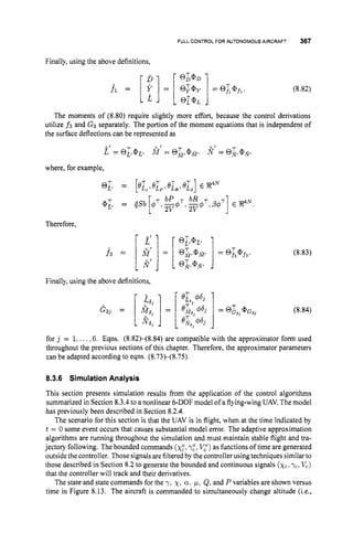
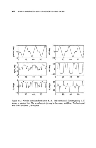
![FULL CONTROLFOR AUTONOMOUS AIRCRAFT 369
nonzero y) and turn (i.e., time-varying x)while holding airspeed constant and regulating
sideslip to zero, i.e., coordinated turns. This type of command is relatively challenging for
the autopilot because it induces significant amounts of coupling between all three channels
and requires flight at high roll angles. In Figure 8.13, the commanded state is plotted as a
dotted curve while the actual state is plotted as a solid curve. The tracking error is clearly
evident near t = 0 for the variables y,a,and Q.
0 20 40 60
L
0 20 40 60
L I
0 20 40 60
“I I
I I
0 20 40 60
r n
20
-5‘ 1
0 20 40 60
-20L 1
0 20 40 60
Figure 8.14: Aircraft compensated tracking error E for Section 8.3.6. The horizontal axis
shows the time, t,in seconds.
Figure 8.14 plots the compensated tracking error for the y: x,a: p, Q, and P
variables. Within about 10 s, the controller has learned the lift and Q-moment functions
sufficiently well sothat it can command the correct cv and achieve that cv via Q so that the y
command istracked accurately. The p and Ptracking errors are initially large,but decreased
dramatically over the first 75 s of the simulation. For this time period, ~ ( t )
E [2.0,5.0]
degrees and hl E [0.445,0.4651. Therefore, learning has only occurred over a small part
of the operating envelope defined by V.
Figure 8.15 shows the surface positions measured in degrees. The main purpose of these
graphs is to illustrate the reasonableness in terms of magnitude andbandwidth of the control
signals. Accurate tracking has been achieved, in spite of large modeling error, via adaptive
approximation methods without resorting to high-gain or switching control methods.
The control gains were K1 = diag(0.3,0.3,0.2), K2 = diag(2:2,2),and K3 =
diag(l0,30:10). Therefore, X K = 0.2. In the parameter adaptation dead-zone, j ( ~ l ( 2
=
0.02; therefore, parameter adaptation stops- when (l.i1/2 < 0.1. Projection was used to
enforce sign constraints on the elements of G, but not upper bound constraints. The region
V, = [-6,141 deg, E , = 1.0”,and V
: = [-7,151 deg. The quantity = 0 . 2 y .](https://image.slidesharecdn.com/adaptive-approximation-based-controlcompress-230219164415-f6eb4a64/85/adaptive-approximation-based-control_compress-pdf-387-320.jpg)
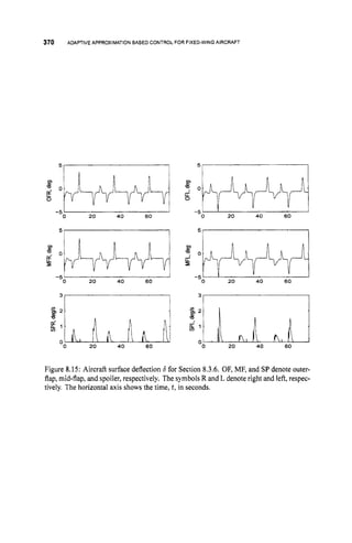
![AIRCRAFT NOTATION 371
Commandvariable
Filter bandwidth, w,
x y V p cr 0 P Q R
1.3 1.3 0.2 6 6 6 100 100 100
The purpose of the command filters for this simulation is only to compute a command
and its derivative; however, the bandwidth of the command filter will influence the state
trajectory. If, for example, 7,"were a step command, then as the bandwidth of the y-
command filter is increased, the magnitude of +c will increase. This will result in larger
changes in Q
, and hence Qc and 6. Similar comments apply to x:, p,, P, and R. The
command filter parameters used for the simulation in this section are given in Table 8.1.
The damping factor in each filter was 1.O.
8.3.7 Conclusions
This section has been concerned with the problem of designing an aircraft control system
capable of tracking ground track, climb rate, and speed commands from a mission planner
while being robust to initial model error as well as changes to the nonlinear model that
might occur during flight due to failures and battle damage. This section derives the aircraft
controller using the command filtered backstepping approach with adaptive approximation
to achieve robustness to unmodeled nonlinear effects, even if those effects change during
flight. The stability properties are proved using Lyapunov methods. The control law and
its stability properties are summarized in Section 8.3.4.
8.4 AIRCRAFT NOTATION
This section is provided as a resource to the reader. Table 8.2 defines the meaning of
the constants that appear in the dynamic equations of the aircraft. Table 8.3 defines the
interpretation of the symbols used to represent the state and control variables. Table 8.4
definesthe unknown and approximate force and moment functions that appear in the model
and control equations.
Figures 8.16 and 8.17 illustrate the definitions of the state related variables.
Symbol Meaning
Mass
Vertical gravity component
Rotational inertia parameters defined on p. 80 in [258]
Reference wing span
Mean geometric chord
Wing reference area
Table 8.2: Definitions of Constants](https://image.slidesharecdn.com/adaptive-approximation-based-controlcompress-230219164415-f6eb4a64/85/adaptive-approximation-based-control_compress-pdf-389-320.jpg)

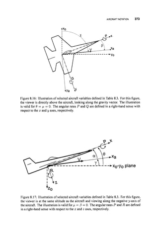
![374 ADAPTIVE APPROXIMATION BASED CONTROL FOR FIXED-WING AIRCRAFT
Problems
Exercise 8.1 Consider the very simple system 5 = f* +u with z E 'D = [-2,2] C R1
and f* = 1
x
1-1being unknown at the design stage. Even though it is obviously not a good
choice, assume that the designer has selected the approximator be f^ = 80 +012 = eT4(z)
where $(z) = [l,zIT.
1. Use (2.35) to show that the least squares optimal parameter estimate over 'D is
O* = [0,0IT. The C
, optimal estimate over 2)is also 8* = [0,0IT. Therefore,
rnaxzED (ief(z)i) = 1.0 = df where ef(z)= f*(z)- f(z).
2. Show that for any operating point z+ E '
D such that z+ > 0, there is a closed
neighborhood of z+ on which f * is perfectly approximated with 6; = -1:I].
Similarly, for z- E 'D such that z- < 0, there is a closed neighborhood of z-
on which f" is perfectly approximated with 0: = [-1,-11. For later use, define
0+=8-8;andO- =8-8?.
update equations as
3. Following the basic procedure of Section 8.2.3,define the control law and parameter
3 = { " ifK/i?/> E
0 otherwise
where z
, and i,are the commanded state trajectory and its time derivative.
(a) Show that the tracking error dynamics are
2 = -ijT$- KZ+ef(z)+VD.
(b) Show that, for K/Zl > E and z E 'D, the time derivative of the Lyapunov
function v = i? +BTr-16) satisfies
(
v I
-13 (KFl- lerl).
Therefore, when E < Kl3/ < / e f /it is possible for the positive function V to
increase.
4. SimulatethesysternandgenerateplotsofV(t),V+(t)= $ (2 +6lI?-'8+),V-(t)=
(2 +6?I'-'6-), and (K12.j- lefl). Use the control gain K = 4, adaptationrate
I' = 51, dead-zone radius E = 0.01, and command filter parameters wn = 15,
( = 1.0 (see eqn. (8.14)). Let zz = 0.8sin(t)+T ( t ) where r(t)is a square wave
switching between *l.O with a period of 50 s.
From these plots, you should notice the following: (a) V ( t )is decreasing when
(K/Z- lefl) is positive and increasing otherwise; (b) V+(t)
is decreasing when z
is positive and V- (t)is decreasing when z is negative.
The main conclusion of this exercise is that when the approximation structure is not
sufficient to guarantee learning (Lea,Ef > E ) then the approximator parameters will](https://image.slidesharecdn.com/adaptive-approximation-based-controlcompress-230219164415-f6eb4a64/85/adaptive-approximation-based-control_compress-pdf-392-320.jpg)

![APPENDIX A
SYSTEMS AND STABILITY CONCEPTS
This appendix presents certain necessary concepts that are used in the main body of the
book. This material is presented in the form of an appendix, as it may be familiar to many
readers and will therefore not interrupt the main flow of the text. Proofs are not included.
Proofs canbe found in [119,134,169,249], which are the main references for this appendix.
A.l SYSTEMS CONCEPTS
Many dynamic systems (all those of interest herein) can be conveniently represented by a
finite number of coupled first-order ordinary differential equations:
w h e r e x ~ S F Z n , u ~ S F Z m ~ , y ~ S F Z ~ , f o : ~ n x S F Z m x ~ 1 ~ ~ n , a n d h o : ~ n x ~ m x ~
++SFZP.
The parameter n is referred to as the system order. The vector z is referred to as the system
state. The vector space SFZn over which the state vector is defined is the state space.
In the special case where u(t)is a constant and fo is not an explicit fimction oft, then
eqn. (A.1)simplifies to
This equation, which is independent of time, is said to be autonomous,
Adaptive Approximation Based Control:Uni5ing Neural,Fuzqv and TraditionalAdaptive 377
Approximation Approaches.By Jay A. Farrell and Marios M. Polycarpou
Copyright @ 2006 John Wiley & Sons,Inc.](https://image.slidesharecdn.com/adaptive-approximation-based-controlcompress-230219164415-f6eb4a64/85/adaptive-approximation-based-control_compress-pdf-395-320.jpg)
![378 SYSTEMSAND STABILITYCONCEPTS
Solutions. The analyst is often interested in qualitative properties of the solutions of the
system ofequations defined by eqn. (A.1). For a given signal u(t),a solution to eqn. (A.1)
over an interval t E [to,tl]is a continuous function x(t) : [to,tl] Rn such that x(t)is
defined and j ( t )= f,(z(t),u(t),t )for all t E [to,t l ] .The solution x(t) traces a curve in
Rn as t varies from toto tl. This curve is the state trajectory.
Existence and Uniqueness of Solutions. The two questions of whether a differential
equation has a solution and, if so, whether it is unique are fundamental to the study of
differential equations. Discussion of the uniqueness of a solution requires introduction of
the concept of the Lipschitz condition.
Definition A.l.l Afunction f satisfies a Lipschitz condition on V with Lipschitz constant
llf(tlx)- f(tl Y)li 5 YIIX - YII
rif
for allpoints (t,z) and (tly) in V.
Lipschitz continuity is a stronger condition that continuity. For example, f(z) =
xPl for 0 < p < 1, is a continuous function on V = [O,m],but it is not Lipschitz
continuous on V since its slope approaches infinity as z approaches zero.
The following theorem summarizes the conditions required for local existence and
uniqueness of solutions.
Theorem A.1.1 [134] rf f(t,x) ispiecewise continuous in t and satisfies a Lipschitz con-
dition on a compact set containing x(t0).then there exists some S > 0 such that the initial
valueproblem
x = f(t,z), with z(t,-,)= zo
has a unique solution on [to,to +61.
Consider, as an example, the initial value problem
x = zp, with z(0) = 0 and 0 <p < 1.
The previous discussion has already shown that f(z)= xp is not Lipschitz. Therefore, the
previous theorem does not guarantee uniqueness of the solution to the initial value problem.
In fact,
z ( t ) = O a n d x ( t ) = ( ( l - p ) t ) h
are both valid solutions to the initial value problem.
Throughout themain body ofthis text, it will often be the casethat solutions ofthe system
equations can be shown to lie entirely in a compact set V.In such cases, the following
theorem is applicable.
Theorem A.1.2 [134] Let f (t,x)be piecewise continuous in t and locally Lipschitz in x
for all t > toand all 2 E A c Rn,where A is a domain containing the compact set V.I
f
for x, E V it is known that every solution of
i = f(t,x), with z(t0)= $0
lies entirely within V,
then there is a unique solution definedfor all t 2 to.
EquilibriumPoint. Letu(t) = Oforallt E ?
I
?
+
.
Anypointz, E Wsuchthatf(z,,O,t) =
0 for all t 6 R+ is an equilibrium point of eqn. (A.1). Conceptually, an equilibrium point](https://image.slidesharecdn.com/adaptive-approximation-based-controlcompress-230219164415-f6eb4a64/85/adaptive-approximation-based-control_compress-pdf-396-320.jpg)
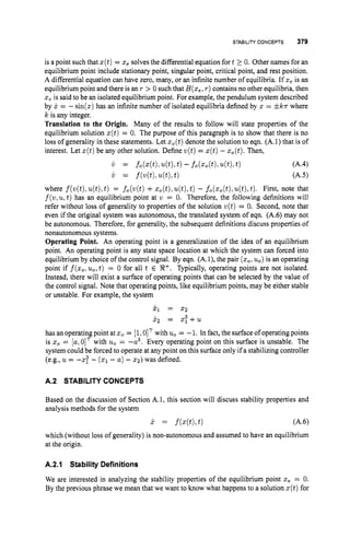
![382 SYSTEMSAND STABILITYCONCEPTS
graphical analysis of trajectories is not possible. Lyapunov's direct method provides these
tools, without the need to explicitly solve for the solution of the differential equation.
The key idea of Lyapunov's direct approach is that the analyst define closed contours
in R" that correspond to the level curves of a sign definite function. The analysis then
focuses on the behavior of the system trajectories relative to these contours. The ideas
of Lyapunov's direct method are rigorously summarized by the Theorem A.2.1. Before
presenting that theorem, we introduce a few essential concepts. In the following definition,
B(T)
denotes an open set containing the origin.
Definition A.2.3
1. A continuousfunction V ( x )ispositive definite on B(r)if
(a) V(0)= 0, and
(b) V ( z )> 0, Vx E B(T)
such that z# 0.
2. A continuousfunction V ( x )ispositive semidefinite on B(r) if
(a) V(0)= 0, and
(b) V ( z )2 0, Vx E B(T)
such that x # 0.
3. A continuousfunction V ( x )i
s negative (semi-)definite on B(r)if-V(x) ispositive
(semi-)definite.
4. A continuousfunction V ( x )i
s radially unbounded i
f
(a) V ( 0 )= 0,
(c) V ( x )+ mas 1
]
5
1
1+ m.
(b) V > 0 on Rn - {0},and
5. A continuousfunction V(t,x)ispositive definite onRx B(r)ifthere exists apositive
definitefunction w( x )on B(T ) such that
(a) V(t,0) = 0,V t 2 0, and
(b) V ( t , x )2 ~ ( x ) ,
V t 2 OandVx E B(T).
6. A continuous function V ( t ,x ) is radially unbounded if there exists a radially un-
boundedfunction w(z)
(a) V(t,O)= 0,Vt 2 0, and
(b) V ( t , z )2 w(x):V t 2 0 andVz E R".
7. A continuousfunction V(t,
x) i
s decrescent on R x B(r)i
f there exists a positive
definitefunction ~ ( x )
on B(T)
such that
V ( t , x )5 ~ ( z ) ,
Vt 2 0 andVx E B(r).
The concept of positive definiteness is important since positive definite functions char-
acterize closed contours around the origin in R". If the time derivative of a positive definite
function V along the system's trajectories can be shown to always be negative, then the
trajectories are only crossing contours in the direction towards the origin. This fact can](https://image.slidesharecdn.com/adaptive-approximation-based-controlcompress-230219164415-f6eb4a64/85/adaptive-approximation-based-control_compress-pdf-400-320.jpg)
![384 SYSTEMS AND STABILITY
CONCEPTS
Let V ( x )= xTP x, where P is a symmetric and positive definite matrix.' Then,
e
l = x ~ ~ ~ ~ x + x ~ ~ ~ x
dt (A.9)
= xT ( A ~ P + P A ) X
-
- -xTQx
where
Q = - ( A ~ P + P A ) (A.10)
is a symmetric matrix. If Q is positive definite, then the linear system is globally2
exponentially stable.
If Q is not positive definite, then nothing can be said about the stability properties
of the system. The fact that Q is not positive definite may be the result of a poor
choice of P for the problem of interest. Therefore, the method of selecting P and
calculating Q = - (ATP +P A) is not the preferred approach.
The equation Q = - (ATP+P A) is referred to as the continuous-timeLya-
punov equation. Note that if Q is specified and A is known, then the Lyapunov
equation is linear in P. Therefore the preferred approach is (1) to specify a positive
definite Q,and (2) to solve the Lyapunov equation for P. If the resulting P is posi-
tive definite, then the linear system is exponentially stable. Ifthe resulting P has any
n
negative eigenvalue, then the linear system is unstable.
EXAMPLEA.2
Consider the example of the pendulum described by
x, = 2 2
x2 = -sin(x1)- xz.
The total energy for this system is
1
2
E(x1,x2) = lzl
sin(v)dv +-x;.
For solutions of the eqn. (A.1I),
dE
-
dt = (VE)T.[ ]
(A.11)
(A.12)
(A.13)
= -x; 5 0, VXl,2 2 . (A.14)
Therefore, the function E is positive definite for x1 E (-n,n),Vx2 E R
'
, with a
negative semidefinite derivative. The conclusion by Theorem A.2.1 is that the system
is uniformly stable.
' A symmetric matrix has all real eigenvalues. If all these eigenvalues are positive, then the matrix is positive
definite.
'The region B(r)in Theorem A.2.1 has T = oc.](https://image.slidesharecdn.com/adaptive-approximation-based-controlcompress-230219164415-f6eb4a64/85/adaptive-approximation-based-control_compress-pdf-402-320.jpg)
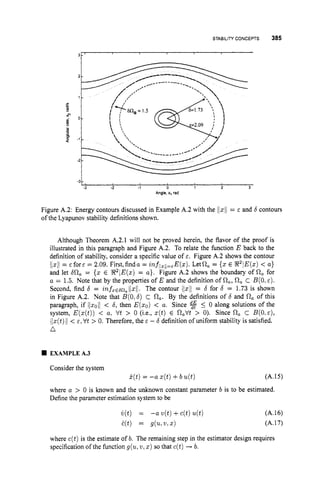

![STABILITY CONCEPTS 391
The time derivative of V along solutions of the above system while lej > 2 is
v = -ke2 +eE.
To show MSS, we choose y E (0,
k ) and complete the square on the right hand side:
5 -(k -y)e2 +-
€2
47
€ 2
47
(k-y)e2 5 -v+ -
where we have assumed that le(0)l > 5 (without loss of generality). From this we can
conclude thate E S
A.2.3 Strictly PositiveReal Transfer Functions
The concepts of Positive Real (PR) and Strictly Positive Real (SPR) ,which are useful in
some forms of stability analysis, are derived from network theory, where a rational transfer
function is the driving point impedance of a network that does not generate energy if and
only if it is PR. A network that does not generate energy is known as a passive or dissipative
network, and it consists mainly of resistors, inductors and capacitors.
Specifically,a rational transfer function W (s)of the complex variable s = u+j w is PR
if W(s)is real for real s, and Re[W(s)] 2 0 for all Re[s] 2 0. A transfer function W ( s )
is SPR if for some E > 0, W ( s- E ) is PR.
The following result of Ioannou and Tao [1201provide frequency domain conditions for
SPR transfer functions.
Lemma A.2.7 A strictlyproper transferfunction W(s)i
s SPR ifand only if
1. W( s )i
s stable;
2. Re[W(jw)]
> 0,for all w E (-m, m); and
3. lim~u~+m
w2Re[W(jw)]
> 0.
It is clear that the class of SPR transfer functions is a special class of stable transfer
functions, which also satisfy a minimum phase condition. The following exampleillustrates
the class of SPR transfer functions for a second order system.
EXAMPLEA.8
Consider the transfer function](https://image.slidesharecdn.com/adaptive-approximation-based-controlcompress-230219164415-f6eb4a64/85/adaptive-approximation-based-control_compress-pdf-409-320.jpg)
![TRAJECTORY GENERATIONFILTERS 395
+ 2 L
Yc +
-
0,...,r is continuous and bounded as it is a state of a stable linear filter with a bounded
input. Note that yd(t) and its first r derivatives are produced without differentiation3.
The transfer function from yc to Yd is
a0
- -
yd(s) - H(s)=
Sn +an-lsn--l + ...+a1s +a0
which has unity gain at low frequencies. Therefore, the error Iyd(t) - yc(t)l is small if the
bandwidth of Yc(s)
is less than the bandwidth of H(s).If the bandwidth of yc is specified
and the only goal of the filter is to generate Y d and its necessary derivatives with jyd - ycl
small, then the designer simply chooses the H ( s )as a stable filter with sufficiently high
bandwidth. However, there are typically additional constraints.
2cw*
EXAMPLEA.9
derivative generation and Iyd - ycl small when the maximum bandwidth of Yc(s)is
specified to be 5 H z ,then any positive value of C and wn > 30% should suffice. A
For many advanced control methods the objective is to design the feedback control law
so that the plant state z(t)E RTwill track the reference trajectory zr(t)= [yd(t), ... ,yr’]
perfectly. Perfect tracking has two conditions. First, if z(0) = zr(0),then z(t)= zT(t)
for any t 2 0. Second, if z(0) # zT(0),then e(t) = z(t)- zr(t)should converge to
zero exponentially (see p. 217 in [249]). If 5 tracks z, perfectly, then the transfer function
H ( s )of the prefilter defined in eqn. (A.26) largely determines the bandwidth required for
the plant actuators and does determine the transient response to changes in yc. In some
applications, this transient response is critically important. For example, in aircraft control
it is referred to as handling qualities and has its own literature. Therefore the choice of
the parameters [ao,al,a2, ...,a,-l], and the pole locations of H ( s )that they determine,
should be carefully considered.
3Notethat the approach described herein is essentially the same as that described in eqns. (7.31) and (7.42). For
example, in eqn. (7.31):
with A and B is definedon page 295. If T is selected as
X d = A X d +BT,
n
T = we- Ca,-,x,t
1=1
then both approaches yield identical results.](https://image.slidesharecdn.com/adaptive-approximation-based-controlcompress-230219164415-f6eb4a64/85/adaptive-approximation-based-control_compress-pdf-413-320.jpg)
![396 SYSTEMS AND STABILITY CONCEPTS
EXAMPLE A.IO
In the case that n = 2 and T = 1that was considered in Example A.9, if the control
specification is for yc defined as a step function to be tracked with less than 5%
overshoot with rise time T,. E [O.l, 0.21 s and settling time to within 1%of its final
value in T, < 0.5 s, then appropriate pole locations are p = -10 fj5, which are
achieved for a. = 125 and al = 20. The selection of pole locations to achieve time
domain specifications is discussed in for example Section 3.4 in 1861.
The trajectory output by the prefilter will achieve the time domain tracking spec-
ification. The prefilter is outside of the feedback control loop. If the feedback
controller achieves perfect tracking, then the state of the plant will also achieve the
tracking specification. n
Finally, in adaptive approximation based control, the desired trajectory is assumed to
remain in the operating region denoted by V.This assumption can also be enforced by a
suitable trajectory prefilter design, as shown in the following example.
EXAMPLE A.ll
In the case that n = 2 and T = 1 that was considered in Example A.9, assume
that V = [y,B] x [gl
?i] and an additional constraint on the prefilter is to ensure that
(yd(t)r y d ( z ) ) E v trt 2 0,assuming that (&(0)lyd(0)) E V.A filter designed to
help enforce this constraint is
where
Ye,@) = 9 (YC(tL&B).
The saturation function indicated by g is defined as
z i f s z z
i-
x ifxs:.
g(z,:,Z) = 2 i f g 2 2 Iz
This filter is depicted as a block diagram format in Figure AS.
The signal yel(t)is a magnitude limited version of yc(t).Thisensures that the user
does not inadvertently command Yd to leave [g,
- g].The signal ycl is interpreted as the
commanded value for z1 = yd. The error (yo - &) is multiplied by the gain 2and
limited to the range [g?
a]to produce the signal v,~that is treated as the commanded
value for z2 = yd.
Note that even such a filter does not guarantee that (Yd(t)l y d ( t ) ) E V V t 2 0,
because z2 will lag we,. Therefore, the region enforced by the command filter should
n
be selected as a proper subset of the physical operating envelope.](https://image.slidesharecdn.com/adaptive-approximation-based-controlcompress-230219164415-f6eb4a64/85/adaptive-approximation-based-control_compress-pdf-414-320.jpg)
![A USEFUL INEQUALITY 397
Figure AS: Trajectory generation prefilter for Example A.11 that ensures ~ d ( t )
E [y!
- jj]
and yd(t) E [g!
7
4
.
A.5 A USEFUL INEQUALITY
Most of the bounding techniques that are developed and used throughout the book require
the use of a switching, or signum function sgn(E), which is discontinuous at < = 0. In
order to avoid hard switching in the control or adaptive laws, it is desirable to use a smooth
approximation of the signum function. The following result presents a useful inequality for
using the function tanh(c/a) as a smooth approximation to sgn(6).
Lemma A.5.1 Thefollowing inequalityholdsfor any E > 0 andfor any ,
$ E R'
(A.28)
where K i
s a constant that satisfies K = e-("+l); j.e., IC = 0.2785,
Proof: By dividing throughout by E, proving (A.28) is in fact equivalent to
0 5 111 - ztanh(z) 5 IC! 2 E 3' (A.29)
where z = < / E . Let
M ( z )= /zI - z tanh(z).
Since M(-z) = M ( z )(i.e., M is an even function), we only need to consider the case of
z 2.0. Moreover, we note that M(0)= 0, so for z = 0 (A.29) holds trivially. Hence, it is
left to show that for positive z we have 0 5 M ( z )5 K. For z > 0,
M ( z )= z(1 - tanh(z)),
and therefore M ( z ) 2 0. To prove that M ( z )5 IC we note that M ( z )has a well-defined
maximum (see Figure A.6). To determine the maximum, we take the derivative and set it
to zero, which yields
dM e z -e-2
-
dz = dz
L{+-)}ez +cZ
(I-2z +e-") = 0.
Hence, the value z = z* that achieves the maximum satisfies
2
(ez +e-z)2
-
-
e-2'' = 22" - 1.](https://image.slidesharecdn.com/adaptive-approximation-based-controlcompress-230219164415-f6eb4a64/85/adaptive-approximation-based-control_compress-pdf-415-320.jpg)
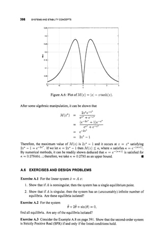


![Ph robust-and-optimal-control-kemin-zhou-john-c-doyle-keith-glover-603s[1]](https://cdn.slidesharecdn.com/ss_thumbnails/ph-robust-and-optimal-control-kemin-zhou-john-c-doyle-keith-glover-603s1-150521042530-lva1-app6891-thumbnail.jpg?width=640&height=640&fit=bounds)