3. TG-43 were as large as 17% for some sources. These
changes have been exhaustively reviewed by the physics
community and are generally accepted. Most treatment plan-
ning software vendors have implemented the TG-43 formal-
ism and the recommended dosimetry parameters in their sys-
tems. LiF TLD dose measurements and Monte Carlo dose
calculations have largely replaced the semi-empirical dose-
calculation models of the past.
Since publication of the TG-43 protocol over nine years
ago, significant advances have taken place in the field of
permanent source implantation and brachytherapy dosimetry.
To accommodate these advances, the AAPM deemed it nec-
essary to update this protocol for the following reasons:
͑a͒ To eliminate minor inconsistencies and omissions in
the original TG-43 formalism and its
implementation.4–6
͑b͒ To incorporate subsequent AAPM recommendations,
addressing requirements for acquisition of dosimetry
data as well as clinical implementation.7
These recom-
mendations, e.g., elimination of Aapp ͑see Appendix E͒
and description of minimum standards for dosimetric
characterization of low-energy photon-emitting brachy-
therapy sources,8,9
needed to be consolidated in one
convenient document.
͑c͒ To critically reassess published brachytherapy dosime-
try data for the 125
I and 103
Pd source models introduced
both prior and subsequent to publication of the TG-43
protocol in 1995, and to recommend consensus datasets
where appropriate.
͑d͒ To develop guidelines for the determination of
reference-quality dose distributions by both experimen-
tal and Monte Carlo methods, and to promote consis-
tency in derivation of parameters used in TG-43 for-
malism.
Updated tables of TG-43 parameters are necessary and
timely to accommodate the ϳ20 new low-energy interstitial
brachytherapy source models that have been introduced to
the market since publication of TG-43 in 1995. These com-
mercial developments are due mostly to the rapid increase in
utilization of permanent prostate brachytherapy. Some of
these new brachytherapy sources were introduced into clini-
cal practice without thorough scientific evaluation of the nec-
essary dosimetric parameters. The AAPM addressed this is-
sue in 1998, recommending that at least one experimental
and one Monte Carlo determination of the TG-43 dosimetry
parameters be published in the peer-reviewed literature be-
fore using new low-energy photon-emitting sources ͑those
with average photon energies less than 50 keV͒ in routine
clinical practice.9
Thus, many source models are supported
by multiple dosimetry datasets based upon a variety of basic
dosimetry techniques. This confronts the clinical physicist
with the problem of critically evaluating and selecting an
appropriate dataset for clinical use. To address this problem,
this protocol presents a critical review of dosimetry data for
eight 125
I and 103
Pd source models which satisfied the afore-
mentioned criteria as of July 15, 2001, including the three
low-energy source models included in the original TG-43
protocol. The present protocol ͑TG-43U1͒ recommends a
single, consensus dataset for each source model from which
the 1D and 2D dose-rate distribution can be reconstructed.
͓This protocol was prepared by the AAPM Low-energy In-
terstitial Brachytherapy Dosimetry subcommittee, now the
Photon-Emitting Brachytherapy Dosimetry subcommittee
͑Chair, Jeffrey F. Williamson͒ of the AAPM Radiation
Therapy Committee. This protocol has been reviewed and
approved by the AAPM Radiation Therapy Committee and
AAPM Science Council, and represents the current recom-
mendations of the AAPM on this subject.͔ Finally, method-
ological guidelines are presented for physicist-investigators
aiming to obtain dosimetry parameters for brachytherapy
sources using calculative methods or experimental tech-
niques.
Although many of the principles and the changes in meth-
odology might apply, beta- or neutron-emitting sources such
as 90
Sr, 32
P or 252
Cf are not considered in this protocol. A
further update of this protocol is anticipated to provide con-
sensus, single source dose distributions and dosimetry pa-
rameters for high-energy photon-emitting ͑e.g. 192
Ir and
137
Cs) sources, and to generate consensus data for new low-
energy photon sources that are not included in this report, yet
meet the AAPM prerequisites and are posted on the AAPM/
RPC Seed Registry website10
as of December 1, 2003:
͑1͒ Amersham Health, OncoSeed model 6733 125
I,
͑2͒ Best Medical model 2335 103
Pd,
͑3͒ Draximage Inc., BrachySeed model LS-1 125
I,
͑4͒ IBt, Intersource-125 model 1251L 125
I,
͑5͒ IBt, Intersource-103 model 1031L 103
Pd,
͑6͒ Implant Sciences Corp. I-Plant model 3500 125
I,
͑7͒ IsoAid, Advantage model 1A1-125A 125
I,
͑8͒ Mills Biopharmaceuticals Inc., ProstaSeed model SL/
SH-125 125
I,
͑9͒ Nucletron Corp., selectSeed model 130.002 125
I, and
͑10͒ SourceTech Medical, 125
Implant model STM1251 125
I.
As indicated in the Table of Contents, this protocol is
divided into various sections. Clinical medical physicists
should pay special attention to Secs. III–VI due to dosimetry
formalism and clinical implementation recommendations
presented herein. Section II updates the clinical rationale for
accurate dosimetry. The origin of consensus datasets for
eight seed models is presented in Appendix A. Dosimetry
investigators will find useful the detailed recommendations
presented in Secs. IV and V. The description of the NIST
calibration scheme is presented in Appendix B. Manufactur-
ers of brachytherapy treatment planning software will find
new recommendations in Secs. II, IV, VI, and Appendixes
C–E.
II. CLINICAL RATIONALE FOR ACCURATE
DOSIMETRY
While low-energy, photon-emitting brachytherapy sources
have been used to treat cancers involving a variety of ana-
tomical sites, including eye plaque therapy for choroidal
635 Rivard et al.: AAPM TG-43 update 635
Medical Physics, Vol. 31, No. 3, March 2004
4. melanoma and permanent lung implants,11,12
their most fre-
quent indication today is for the treatment of prostate
cancer.13
Prostate cancer is the most frequent type of cancer
in men in the United States with approximately 180 000 new
cases incident per year and an annual death rate of about
37 000.14
While approximately 60% of new cases are con-
fined to the organ at time of diagnosis, only about 2.2% of
these new cases were treated with brachytherapy in 1995.
Since that time, the percentage has increased to about 30% of
all eligible patients receiving implants in current practice.
This increase was largely due to improvements in diagnosis
and case selection facilitated by introduction of the prostate
specific antigen ͑PSA͒ screening test, and to improved
ultrasound-guided delivery techniques. In the United States,
the pioneering work was performed by a group of investiga-
tors based in Seattle.15
The most widely used technique uti-
lizes transrectal ultrasound ͑TRUS͒ guided implantation of
either 125
I or 103
Pd brachytherapy sources using a template-
guided needle delivery system to avoid open surgery re-
quired by the retropubic approach.16,17
Several studies have shown that clinical outcomes in pros-
tate brachytherapy, both for the retropubic approach and the
TRUS-guided technique, correlate with dose coverage pa-
rameters. The extensive clinical experience of Memorial
Sloan Kettering Institute ͑1078 patients with retropubic ap-
proach surgery͒ from 1970–1987 was reviewed by Zelefsky
and Whitmore.18
Multivariate-analysis revealed a D90 im-
plant dose of 140 Gy to be an independent predictor of
recurrence-free local control at 5, 10, and 15 years (p
ϭ0.001). D90 is defined as the dose delivered to 90% of the
prostate volume as outlined using post-implant CT images.
Similarly, a review of 110 implants at Yale University using
the retropubic implant approach from 1976 to 1986 reported
a correlation (pϭ0.02) of recurrence-free local control after
10 years with V100 ; V100 is defined as the percentage of
target volume receiving the prescribed dose of 160 Gy.19
Two recent retrospective studies of the TRUS technique
demonstrate that the clinical outcome depends on dose deliv-
ered and prostate volume coverage. Stock et al. reported on
an experience of 134 prostate cancer patients implanted with
125
I and not treated with teletherapy or hormonal therapy.20
They assessed rates of freedom from biochemical failure as a
function of the D90 dose. A significant increase in freedom
from biochemical failure ͑92% vs 68% after 4 years͒ was
observed (pϭ0.02) for patients (nϭ69) where D90
у140 Gy. Potters et al. recently reviewed the impact of vari-
ous dosimetry parameters on biochemical control for their
experience of 719 patients treated with permanent prostate
brachytherapy.21
Many of these patients also received tele-
therapy ͑28%͒ or hormone therapy ͑35%͒. Furthermore, 84%
of the implants used 103
Pd with the remainder using 125
I.
Their results indicated that patient age, radionuclide selec-
tion, and use of teletherapy did not significantly affect bio-
chemical relapse-free survival ͑PSA–RFS͒. The only dose-
specification index that was predictive of PSA–RFS was
D90 .
Like the other two studies, studies by Stock et al. and
Potters et al. were based on pre-TG-43 prescription doses of
160 Gy, and both indicated a steep dependence of clinical
outcome with dose in the range of 100 to 160 Gy. For ex-
ample, Stock reported freedom from biochemical failure
rates of 53%, 82%, 80%, 95%, and 89% for patients receiv-
ing D90Ͻ100 Gy, 100рD90Ͻ120 Gy, 120рD90Ͻ140 Gy,
140рD90Ͻ160 Gy and D90у160 Gy, respectively. The close
correlation between D90 and PSA–RFS, and a dose response
in the clinical dose range of 100 to 160 Gy are strong justi-
fications for improved accuracy in the dosimetry for intersti-
tial brachytherapy, which is the focus of this work. The up-
dated dosimetry formalism and changes in calibration
standards recommended herein will result in changes to the
clinical practice of brachytherapy. The clinical medical
physicist is advised that guidance on prescribed-to-
administered dose ratios for 125
I and 103
Pd will be forthcom-
ing in a subsequent report.
III. TASK GROUP # 43 DOSIMETRY FORMALISM
As in the original TG-43 protocol, both 2D ͑cylindrically
symmetric line source͒ and 1D ͑point source͒ dose-
calculation formalisms are given. To correct small errors and
to better address implementation details neglected in the
original protocol, all quantities are defined. Throughout this
protocol, the following definitions are used:
͑1͒ A source is defined as any encapsulated radioactive ma-
terial that may be used for brachytherapy. There are no
restrictions on the size or on its symmetry.
͑2͒ A point source is a dosimetric approximation whereby
radioactivity is assumed to subtend a dimensionless
point with a dose distribution assumed to be spherically
symmetric at a given radial distance r. The influence of
inverse square law, for the purpose of interpolating be-
tween tabulated transverse-plane dose-rate values, can be
calculated using 1/r2
.
͑3͒ The transverse-plane of a cylindrically symmetric source
is that plane which is perpendicular to the longitudinal
axis of the source and bisects the radioactivity distribu-
tion.
͑4͒ A line source is a dosimetric approximation whereby ra-
dioactivity is assumed to be uniformly distributed along
a 1D line-segment with active length L. While not accu-
rately characterizing the radioactivity distribution within
an actual source, this approximation is useful in charac-
terizing the influence of inverse square law on a source’s
dose distribution for the purposes of interpolating be-
tween or extrapolating beyond tabulated TG-43 param-
eter values within clinical brachytherapy treatment plan-
ning systems.
͑5͒ A seed is defined as a cylindrical brachytherapy source
with active length, L, or effective length, Leff ͑described
later in greater detail͒ less than or equal to 0.5 cm.
These parameters are utilized by the TG-43U1 formalism
in the following sections.
636 Rivard et al.: AAPM TG-43 update 636
Medical Physics, Vol. 31, No. 3, March 2004
5. A. General 2D formalism
The general, two-dimensional ͑2D͒ dose-rate equation
from the 1995 TG-43 protocol is retained,
D˙ ͑r,͒ϭSK•⌳•
GL͑r,͒
GL͑r0 ,0͒
•gL͑r͒•F͑r,͒, ͑1͒
where r denotes the distance ͑in centimeters͒ from the center
of the active source to the point of interest, r0 denotes the
reference distance which is specified to be 1 cm in this pro-
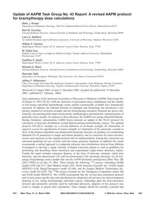
tocol, and denotes the polar angle specifying the point-of-
interest, P(r,), relative to the source longitudinal axis. The
reference angle, 0 , defines the source transverse plane, and
is specified to be 90° or /2 radians ͑Fig. 1͒.
In clinical practice, source position and orientation are
identified by means of radio-opaque markers. Generally,
these markers are positioned symmetrically within the source
capsule such that the marker, the radioactivity distribution,
and the capsule have the same geometric center on the sym-
metry axis of the source. Thus, determination of the location
of the radioisotope distribution is based upon identification
of the radio-opaque markers. All sources discussed in this
document can be accurately represented by a capsule and
radio-opaque markers that are symmetric with respect to the
transverse plane, which by definition bisects the active
source and specifies the origin of the dose-calculation for-
malism. However, Eq. ͑1͒ can accommodate sources that are
asymmetric with respect to the transverse plane. For sources
that exhibit all of the following characteristics: ͑i͒ the radio-
activity distribution is clearly asymmetric with respect to the
planes bisecting the capsule or marker; ͑ii͒ the extent of
asymmetry is known a priori or can be measured via imag-
ing; and ͑iii͒ the source orientation can be determined under
clinical implant circumstances ͑e.g., via CT or radiography͒,
then the source coordinate system origin should be posi-
tioned at the geometric center of the radionuclide distribution
͑as determined using positioning information obtained from
the markers͒, not the geometric center of the exterior surface
of the capsule or marker. If radio-opaque markers do not
facilitate identification of source orientation and the asym-
metrical distribution under clinical circumstances, then the
geometric center of the source must be presumed to reside at
the radio-opaque marker centroid as is conventionally per-
formed.
The quantities used in Eq. ͑1͒ are defined and discussed
later. This formalism applies to sources with cylindrically
symmetric dose distributions with respect to the source lon-
gitudinal axis. In addition, the consensus datasets presented
in Sec. IV B assume that dose distributions are symmetric
with respect to the transverse plane, i.e., that radioactivity
distributions to either side of the transverse plane are mirror
images of one another. However, this formalism is readily
generalized to accommodate sources that are not symmetric
with respect to the transverse plane.
Equation ͑1͒ includes additional notation compared with
the corresponding equation in the original TG-43 formalism,
namely the subscript ‘‘L’’ has been added to denote the line
source approximation used for the geometry function ͑Sec.
III A 3͒. For evaluation of dose rates at small and large dis-
tances, the reader is referred to Appendix C.
1. Air-kerma strength
This protocol proposes minor revisions to the definition of
air-kerma strength, SK , which was first introduced by the
AAPM TG-32 report in 1987.22
Air-kerma strength has units
of Gy m2
h-1
and is numerically identical to the quantity
Reference Air Kerma Rate recommended by ICRU 38 and
ICRU 60.23,24
For convenience, these unit combinations
are denoted by the symbol U where 1 Uϭ1 Gy m2
hϪ1
ϭ1 cGy cm2
hϪ1
.
Air-kerma strength, SK , is the air-kerma rate, K˙
␦(d), in
vacuo and due to photons of energy greater than ␦, at dis-
tance d, multiplied by the square of this distance, d2
,
SKϭK˙
␦͑d͒d2
. ͑2͒
The quantity d is the distance from the source center to the
point of K˙
␦(d) specification ͑usually but not necessarily as-
sociated with the point of measurement͒ which should be
located on the transverse plane of the source. The distance d
can be any distance that is large relative to the maximum
linear dimension of the radioactivity distribution so that SK is
independent of d. K˙
␦(d) is usually inferred from transverse-
plane air-kerma rate measurements performed in a free-air
geometry at distances large in relation to the maximum linear
dimensions of the detector and source, typically of the order
of 1 meter. The qualification ‘‘in vacuo’’ means that the mea-
surements should be corrected for photon attenuation and
scattering in air and any other medium interposed between
the source and detector, as well as photon scattering from
any nearby objects including walls, floors, and ceilings. Of
course, air-kerma rate may also be calculated to subvert
some of the limitations imposed on practical
measurements.25
The energy cutoff, ␦, is intended to exclude
low-energy or contaminant photons ͑e.g., characteristic
x-rays originating in the outer layers of steel or titanium
source cladding͒ that increase K˙
␦(d) without contributing
significantly to dose at distances greater than 0.1 cm in tis-
sue. The value of ␦ is typically 5 keV for low-energy photon-
emitting brachytherapy sources, and is dependent on the ap-
plication.
FIG. 1. Coordinate system used for brachytherapy dosimetry calculations.
637 Rivard et al.: AAPM TG-43 update 637
Medical Physics, Vol. 31, No. 3, March 2004
6. In summary, the present definition of SK differs in two
important ways from the original 1987 AAPM definition.
First, the original AAPM definition of SK did not allow for a
low-energy cutoff. Subsequent experience using free-air
chambers as primary SK standards clearly indicates that fail-
ure to exclude nonpenetrating radiations greatly increases
measurement uncertainty and invalidates theoretical dosime-
try models. Second, the conditions that should prevail in an
experimental determination of SK are now explicitly stated.
2. Dose-rate constant
The definition of the dose-rate constant in water, ⌳, is
unchanged from the original TG-43 protocol: it is the ratio of
dose rate at the reference position, P(r0 ,0), and SK . ⌳ has
units of cGy hϪ1
UϪ1
which reduces to cmϪ2
,
⌳ϭ
D˙ ͑r0 ,0͒
SK
. ͑3͒
The dose-rate constant depends on both the radionuclide and
source model, and is influenced by both the source internal
design and the experimental methodology used by the pri-
mary standard to realize SK .
In 1999, a notation was introduced, ⌳nnD,PqqS , to identify
both the dose-rate measurements or calculations used to de-
termine D˙ (r0 ,0) and the calibration standard to which this
dose rate was normalized. The subscript ‘‘D’’ denotes refer-
ence dose rate, ‘‘nn’’ denotes the year in which this refer-
ence dose rate was published ͑either measurement or calcu-
lation͒, ‘‘P’’ denotes the provider or origin of the source
strength standard ͑e.g., Pϭ‘‘N’’ for NIST, or Pϭ‘‘T ’’ for the
in-house calibration-standard of Theragenics Corporation͒,
‘‘qq’’ denotes the year in which this source strength standard
was implemented, and the ‘‘S’’ subscript denotes the word
standard.7
For example, ⌳97D,N99S indicates a dose-rate con-
stant determined from dosimetry measurements published in
1997 and normalized to an SK traceable to the 1999 NIST
standard. Additional notation may also be utilized such as
TLD
6702
⌳97D,N85S for the dose-rate constant for the model 6702
source published in 1997 using TLDs and the 1985 NIST
standard. These notations are useful for comparing results
from multiple investigators, and readily highlight features
such as utilization of the calibration procedure and whether
or not influence of titanium K-shell x rays is included.
3. Geometry function
Within the context of clinical brachytherapy dose calcula-
tions, the purpose of the geometry function is to improve the
accuracy with which dose rates can be estimated by interpo-
lation from data tabulated at discrete points. Physically, the
geometry function neglects scattering and attenuation, and
provides an effective inverse square-law correction based
upon an approximate model of the spatial distribution of ra-
dioactivity within the source. Because the geometry function
is used only to interpolate between tabulated dose-rate values
at defined points, highly simplistic approximations yield suf-
ficient accuracy for treatment planning. This protocol recom-
mends use of point- and line-source models giving rise to the
following geometry functions:
GP͑r,͒ϭrϪ2
point-source approximation,
͑4͒
GL͑r,͒ϭͭ 
Lr sin
if 0°
͑r2
ϪL2
/4͒Ϫ1
if ϭ0°
line-source approximation,
where  is the angle, in radians, subtended by the tips of the
hypothetical line source with respect to the calculation point,
P(r,).
In principle, either the point-source or line-source models
may be consistently implemented in both the 1D and 2D
versions of the TG-43 formalism. In this case, the word
‘‘consistently’’ means that the geometry function used for
derivation of dose rates from TG-43 parameters should be
identical to that used to prepare the radial dose function and
2D anisotropy function data, including use of the same active
length, L, used in G(r,). Under these conditions, TG-43
dose calculations will reproduce exactly the measured or
Monte Carlo-derived dose rates from which g(r) and F(r,)
tables were derived. This protocol recommends consistent
use of the line-source geometry function for evaluation of 2D
dose distributions, and use of either point- or line-source
geometry functions for evaluations of 1D dose distributions.
Use of such simple functions is warranted since their purpose
is to facilitate interpolation between tabulated data entries for
duplication of the original dosimetry results.
In the case where the radioactivity is distributed over a
right-cylindrical volume or annulus, this protocol recom-
mends taking active length to be the length of this cylinder.
For brachytherapy sources containing uniformly spaced mul-
tiple radioactive components, L should be taken as the effec-
tive length, Leff , given by
Leffϭ⌬SϫN, ͑5͒
where N represents the number of discrete pellets contained
in the source with a nominal pellet center-to-center spacing
⌬S. If Leff is greater than the physical length of the source
capsule ͑usually ϳ4.5 mm), the maximum separation ͑dis-
tance between proximal and distal aspects of the activity dis-
tribution͒ should be used as the active length, L. This tech-
638 Rivard et al.: AAPM TG-43 update 638
Medical Physics, Vol. 31, No. 3, March 2004
7. nique avoids singularities in evaluating G(r,) for points of
interest in tissue which are located on the hypothetical line
source just beyond the tip and end of the physical source.
More complex forms of the geometry function have a role
in accurately estimating dose at small distances outside the
tabulated data range, i.e., extrapolating g(r) and F(r,) to
small distances.26,27
Use of such expressions is permitted.
However, most commercial brachytherapy treatment plan-
ning systems support only point- or line-source geometry
functions. Therefore, it is the responsibility of the physicist
to transform the tabulated TG-43 parameters given in this
protocol, which are based upon point- and line-source ap-
proximations, to a format consistent with more complex ge-
ometry functions that may be available on their treatment
planning systems.28–30
4. Radial dose function
The radial dose function, gX(r), accounts for dose fall-off
on the transverse-plane due to photon scattering and attenu-
ation, i.e., excluding fall-off included by the geometry func-
tion. gX(r) is defined by Eq. ͑6͒, and is equal to unity at r0
ϭ1 cm.
gX͑r͒ϭ
D˙ ͑r,0͒
D˙ ͑r0 ,0͒
GX͑r00͒
GX͑r,0͒
. ͑6͒
The revised dose-calculation formalism has added the sub-
script ‘‘X’’ to the radial dose function and geometry function
to indicate whether a point-source, ‘‘P,’’ or line-source,
‘‘L,’’ geometry function was used in transforming the data.
Consequently, this protocol presents tables of both gP(r) and
gL(r) values.
Equation ͑7͒ corrects a typographical error in the original
TG-43 protocol.31
While table lookup via linear interpolation
or any appropriate mathematical model fit to the data may be
used to evaluate gX(r), some commercial treatment planning
systems currently accommodate a fifth-order polynomial fit
to the tabulated g(r) data. Since this type of polynomial fit
may produce erroneous results with large errors outside the
radial range used to determine the fit, alternate fitting equa-
tions have been proposed which are less susceptible to this
effect,32
gX͑r͒ϭa0ϩa1rϩa2r2
ϩa3r3
ϩa4r4
ϩa5r5
. ͑7͒
Parameters a0 through a5 should be determined so that they
fit the data within Ϯ2%. Also, the radial range over which
the fit meets this specification should be clearly specified.
5. 2D anisotropy function
The 2D anisotropy function, F(r,), is defined as
F͑r,͒ϭ
D˙ ͑r,͒
D˙ ͑r,0͒
GL͑r,0͒
GL͑r,͒
. ͑8͒
Other than inclusion of the subscript L, this definition is
identical to the original TG-43 definition.1
The 2D anisot-
ropy function describes the variation in dose as a function of
polar angle relative to the transverse plane. While F(r,) on
the transverse plane is defined as unity, the value of F(r,)
off the transverse plane typically decreases as ͑i͒ r decreases,
͑ii͒ as approaches 0° or 180°, ͑iii͒ as encapsulation thick-
ness increases, and ͑iv͒ as photon energy decreases. How-
ever, F(r,) may exceed unity at ͉Ϫ90°͉ϾϮarcsin(L/2r)
for right-cylinder sources coated with low-energy photon
emitters due to screening of photons by the active element at
angles towards the transverse plane.
As stated earlier, the active length, L, used to evaluate
GL(r,) in Eq. ͑4͒ shall be the same L used to extract gL(r)
and F(r,) from dose distributions via Eqs. ͑6͒ and ͑8͒,
respectively. Otherwise, significant errors in dosimetry re-
sults at small distances may arise. For example, at r
ϭ0.5 cm, a change in L from 3 to 5 mm results in a 5%
change in GL(r,0).
B. General 1D formalism
While a 1D isotropic point-source approximation ͓Eq. ͑9͔͒
only approximates the true complex 2D dose distribution, it
simplifies source localization procedures by eliminating the
need to determine the orientation of the source longitudinal
axis from imaging studies.
D˙ ͑r͒ϭSK•⌳•
GX͑r,0͒
GX͑r0 ,0͒
•gX͑r͒•an͑r͒. ͑9͒
Users should adopt one of the following implementations of
Eq. ͑9͒:
D˙ ͑r͒ϭSK•⌳•ͩr0
r ͪ2
•gP͑r͒•an͑r͒, ͑10͒
or
D˙ ͑r͒ϭSK•⌳•
GL͑r,0͒
GL͑r0 ,0͒
•gL͑r͒•an͑r͒. ͑11͒
While most treatment planning systems use the implementa-
tions in Eq. ͑10͒, we recommend use of Eq. ͑11͒ due to
improved accuracy at small distances, e.g., rϽ1 cm. Linear
interpolation may be used to match the grid spacing of gX(r)
with the grid spacing of an(r).
These revised formulations require consistency between
the geometry function used for dose calculation and the ge-
ometry function used for extracting gX(r) from the
transverse-plane dose distribution. Furthermore, these re-
vised formulations correct an inconsistency in Eq. ͑11͒ of the
original TG-43 protocol that indirectly recommended the fol-
lowing incorrect equation:
D˙ ͑r͒ϭSK⌳•
GP͑r,0͒
GP͑r0 ,0͒
•gL͑r͒•an͑r͒
͑not recommended͒. ͑12͒
While use of the wrong gX(r) datasets will typically give
errors in the calculated dose rate of less than 2% at distances
beyond 1 cm, average errors of 3%, 15%, and 74% arise at
distances of 0.5, 0.25, and 0.1 cm, respectively. Clinical uti-
639 Rivard et al.: AAPM TG-43 update 639
Medical Physics, Vol. 31, No. 3, March 2004
8. lization of the 1D dosimetry formalism presented in Eq. ͑12͒,
or other formalisms that inconsistently apply the geometry
function, are not recommended.
1. 1D anisotropy function
The 1D anisotropy function, an(r), is identical to the
anisotropy factor defined by the original TG-43 protocol. At
a given radial distance, an(r) is the ratio of the solid angle-
weighted dose rate, averaged over the entire 4 steradian
space, to the dose rate at the same distance r on the trans-
verse plane, see Eq. ͑13͒,
an͑r͒ϭ
͐0
D˙ ͑r,͒sin͑͒d
2D˙ ͑r,0͒
. ͑13͒
Note that one should integrate dose rate, not the values of the
2D anisotropy function to arrive at an(r).
With consistent use of the geometry function, both Eqs.
͑10͒ and ͑11͒ will exactly reproduce the solid-angle weighted
dose rate at a given r. Of the two, Eq. ͑11͒ is recommended
because the line-source geometry function will provide more
accurate interpolation and extrapolation at small distances.
The accuracy achievable using the 1D formalism for prostate
implants was reported by Lindsay et al.,33
and Corbett
et al.34
For brachytherapy treatment planning systems that do not
permit entry of an(r), Eqs. ͑10͒ or ͑11͒ can still be imple-
mented by carefully modifying gX(r) to include an(r) as
shown in Eq. ͑14͒. These modified dosimetry parameters,
gЈ(r) and ¯ anЈ , are defined as
gЈ͑r͒ϭgX͑r͒•an͑r͒,
¯ anЈ ϭ1. ͑14͒
While TG-43 introduced the anisotropy constant, ¯ an ,
LIBD no longer recommends its use. This is discussed in
greater detail in Appendix D.
IV. CONSENSUS DATASETS FOR CLINICAL
IMPLEMENTATION
The 125
I and 103
Pd source models reviewed in this proto-
col ͑Fig. 2͒ satisfied the AAPM recommendations that com-
prehensive ͑2D͒ reference-quality dose-rate distribution data
be accepted for publication by a peer-reviewed scientific
journal on or before July 15, 2001. Appropriate publications
can report either Monte Carlo, or experimentally derived
TG-43 dosimetry parameters. As many as 12 sets of indepen-
dently published data per source model were evaluated dur-
ing preparation for this report. For each source model, a
single consensus dataset was derived from multiple pub-
lished datasets according to the following methodology.35
If
items essential to critical evaluation were omitted, the au-
thors were contacted for information or clarification.
͑a͒ The peer-reviewed literature was examined to identify
candidate dose distributions for each source model de-
rived either from experimental measurements or Monte
Carlo simulations. Experimentally determined values
for the dose-rate constant (EXP⌳) were averaged. Sepa-
rately, ⌳ values obtained using Monte Carlo techniques
(MC⌳) were averaged. The consensus value recom-
mended in this protocol (CON⌳) is the equally
weighted average of the separately averaged experi-
mental and Monte Carlo ⌳ values. In cases where there
is only one experimental result and one Monte Carlo
result: CON⌳ϭ͓EXP⌳ϩMC⌳͔/2.
͑b͒ Each candidate dataset was examined separately and
eliminated from consideration if it was determined to
have a problem, e.g., data inconsistency. Corrections
for use of a nonliquid water measurement phantom
were applied if not included in the original investiga-
tors’ analysis.
͑c͒ For the 2D anisotropy function, F(r,), and the radial
dose function, g(r), all candidate datasets for a given
source model were transformed using identical line-
source geometry functions to permit fair comparison.
The radial dose function was corrected for nonliquid
water measurement medium if necessary. Assuming
that the different datasets agreed within experimental
uncertainties, the consensus data were defined as the
ideal candidate dataset having the highest resolution,
covering the largest distance range, and having the
highest degree of smoothness. For most source models
examined in this protocol, the consensus F(r,) and
g(r) data, CONF(r,) and CONg(r), were taken from
the transformed Monte Carlo dataset.
͑d͒ A few entries in the tabulated consensus datasets were
taken from the nonideal candidate dataset͑s͒ to cover a
larger range of distances and angles. These data were
italicized to indicate that they were not directly con-
firmed by other measurements or calculations.
͑e͒ The 1D anisotropy function, an(r), was derived using
numerical integration of the dose rate, as calculated
from CONF(r,) dataset, with respect to solid angle.
Use of the anisotropy constant, ¯ an , is discouraged as
discussed in Appendix D.
͑f͒ When scientifically justified for a given source model,
exceptions or modifications to these rules were made,
and are described later. For example, if the datasets
were too noisy, they were rejected.
͑g͒ Following tabulation of g(r) and F(r,) for all eight
source models, overly dense datasets were down-
sampled to permit reasonable comparisons. Removal of
a dataset point was deemed reasonable if linear inter-
polation using adjacent points resulted in a difference
no larger than Ϯ2% of the dataset point in question.
Similarly, because the various authors used different
table grids, it was necessary to interpolate some of the
data into the common mesh selected for presenting all
eight datasets. Linear–linear interpolation was used for
F(r,) datasets, and log-linear interpolation was used
for g(r) datasets. Interpolated data are indicated by
boldface.
640 Rivard et al.: AAPM TG-43 update 640
Medical Physics, Vol. 31, No. 3, March 2004
9. The details used to evaluate dosimetry parameters for
each source were the following:
͑1͒ internal source geometry and a description of the source,
͑2͒ review of the pertinent literature for the source,
͑3͒ correction coefficients for 1999 anomaly in NIST air-
kerma strength measurements ͑if applicable͒,
͑4͒ solid water-to-liquid water corrections,
͑5͒ experimental method used, TLD or diode,
͑6͒ active length assumed for the geometry function line-
source approximation,
͑7͒ name and version of the Monte Carlo transport code,
͑8͒ cross-section library used by Monte Carlo simulation,
͑9͒ Monte Carlo estimator used to score kerma or dose, and
͑10͒ agreement between Monte Carlo calculations and ex-
perimental measurement.
A. Source geometry variations
Source geometry and internal construction are highly
manufacturer specific. Source models vary from one another
with regard to weld thickness and type, radioactivity carrier
construction, presence of radio-opaque material with sharp
or rounded edges, the presence of silver ͑which produces
characteristic x rays that modify the photon spectrum͒, and
capsule wall thickness. All of these properties can affect the
dosimetric characteristics of the source. Radioactive carriers
may consist of a radio-transparent matrix, a radio-opaque
object coated with radioactivity, or a radio-transparent matrix
with highly attenuating radioactive coating. For example, the
Amersham model 6702 and NASI model 3631-A/M sources
utilize spherical resin carriers coated or impregnated with
radioactivity. The number of spheres varies from 3 or more
FIG. 2. Brachytherapy seeds examined in this report: ͑a͒ Amersham model 6702 source, ͑b͒ Amersham model 6711 source, ͑c͒ Best model 2301 source, ͑d͒
NASI model MED3631-A/M or MED3633 source, ͑e͒ Bebig/Theragenics Corp. model I25.S06 source, ͑f͒ Imagyn model IS-12501 source, and ͑g͒ Ther-
agenics Corp. model 200 source. The titanium capsule is 0.06 mm thick for the Amersham and Theragenics seeds, while each capsule of the Best seed is 0.04
mm thick. The capsule thickness of the remaining seeds is 0.05 mm.
641 Rivard et al.: AAPM TG-43 update 641
Medical Physics, Vol. 31, No. 3, March 2004
10. per source. Other sources, such as the Amersham model
6711, utilize a silver rod carrier. The amount of silver, or the
length of silver rod, varies by the source model. Graphite
pellets are also used. For example, in the Theragenics Cor-
poration model 200 103
Pd source, the pellets are coated with
a mixture of radioactive and nonradioactive palladium.
All 125
I and 103
Pd source models, except for the now-
obsolete model 6702 source, contain some type of radio-
opaque marker to facilitate radiographic localization. For ex-
ample, the graphite pellets of the Theragenics Corporation
source are separated by a cylindrical lead marker. Beside the
obvious dependence of photon spectrum on the radioisotope
used, the backing material ͑e.g., the radio-opaque marker͒
may further perturb the spectrum. For the sources containing
125
I deposited on silver, the resultant silver x rays signifi-
cantly modify the effective photon spectrum. These source
construction features influence the resultant dose rate distri-
bution and the TG-43 dosimetry parameters to varying de-
grees. Accurate knowledge of internal source geometry and
construction details is especially important for Monte Carlo
modeling. Individual sources are briefly described later. Ref-
erences describing each source and the TG-43 parameters are
given in each section. While Sec. III presented the dosimetry
formalism, its applicability to the derivation of consensus
datasets is given later. A detailed description for seed models
is provided in Appendix A.
B. General discussion of TG-43 dosimetry parameters
1. Air-kerma strength standards
The NIST Wide-Angle Free-Air Chamber or WAFAC-
based primary standard became available in 1998, and was
used to standardize the 125
I sources then available ͑models
6702, 6711, and MED3631-A/M͒. For a more detailed dis-
cussion of the NIST air-kerma strength standards, including
those based on the Ritz free-air chamber ͑1985͒ and WAFAC
͑1999͒, see Appendix B. The WAFAC standard shifted for
unknown reasons in 1999, and was corrected in the first half
of 2000. For those sources available in 1998, the 1998 and
2000 WAFAC measurements agreed within estimated mea-
surement uncertainty. Following restoration of the WAFAC
to its 1998 sensitivity in 2000, all sources initially standard-
ized against WAFAC measurements performed in 1999, and
the model 3631-A/M source, which had renormalized its
stated strength against the WAFAC in 1999, had to be stan-
dardized against the corrected WAFAC measurements. To
implement these corrections, five sources of each type were
calibrated using the NIST WAFAC and then sent to both the
accredited dosimetry calibration laboratories ͑ADCLs͒ and
the manufacturer for intercomparisons with their transfer
standards. The AAPM Calibration Laboratory Accreditation
subcommittee, in conjunction with NIST, selected the NIST
WAFAC calibration date as the reference date for each
source model, converting stated source strengths to the NIST
WAFAC 1999 standard as corrected in 2000. This date, as
described on ADCL calibration reports as the vendor trace-
ability date, gives the date of the WAFAC calibration mea-
surements to which the certified calibration is traceable. All
vendors discussed in this protocol have agreed to accept
these same WAFAC measurements as the basis for their
stated source strengths. Subsequent periodic intercompari-
sons between NIST, ADCL, and vendor calibrations will be
compared to this original reference calibration, but will not
be modified unless large deviations are noted. Table I gives
the NIST standard calibration date that is presently used by
the ADCLs, NIST and the manufacturer for each source
model along with the corresponding correction applied to
CON⌳ values to account for the 1999 WAFAC anomaly. The
⌳ values of Table I have been corrected to the air-kerma
standard specified by the WAFAC measurement performed
on the listed date specified in the table. Generally, intercom-
parisons have agreed within Ϯ2% of the source strengths
derived from the WAFAC measurements listed in Table I.
These standardization dates are subject to revision should
changes in manufacturing procedures, source geometry, or
the WAFAC standard itself occur that affect the accuracy of
vendor or ADCL secondary standards. Future source model-
specific revisions to the calibration standard could require
corresponding corrections to the recommended dose-rate
constant. For this reason, regular calibration comparisons
among NIST, ADCL, and vendors are required.9
In summary, there were two possible situations regarding
the calibration of seeds at NIST using the WAFAC-based
air-kerma strength standard. First, seed calibrations per-
formed at NIST during the 1999 calendar year need correc-
tion due to a measurement anomaly present in 1999 only.
This correction was determined by another WAFAC mea-
surement for each seed model made at a designated date in
2000 or later. Second, WAFAC measurements made prior to
1999 and after January 1, 2000 needed no correction. Since
the notation SK,N99 represents the NIST WAFAC-based air-
kerma strength standard as officially introduced on January
1, 1999, this notation is used for all WAFAC measurements,
regardless of the date of calibration. Thus, all measured
dose-rate constant data given in this protocol have been nor-
malized to the SK,N99 standard. Any measured dose-rate con-
stants normalized to NIST calibrations performed in 1999
have been appropriately corrected for WAFAC measurement
anomalies.
2. Dose-rate constant
Specifying the dose-rate constant as accurately as possible
is essential, as it is used to transform the relative TG-43 dose
distribution into absolute dose rates given the air-kerma
strength of the sources deployed in the patient. As discussed
in more detail in Sec. V E, Monte Carlo simulations have a
freedom from detector positioning and response artifacts,
smaller estimated uncertainty, and can yield artifact-free
dose-rate estimates at distances shorter or longer than those
accessible by TLD measurement techniques. However, the
accuracy of Monte Carlo is inherently limited by the inves-
tigators’ ability to accurately delineate the source internal
geometry. Few Monte Carlo studies have systematically
evaluated the effects of geometric uncertainty, internal com-
ponent mobility, tolerances in the fabrication of sources, and
642 Rivard et al.: AAPM TG-43 update 642
Medical Physics, Vol. 31, No. 3, March 2004
11. small manufacturing changes on the uncertainty of calculated
dose-rate distributions. Therefore, the use of Monte Carlo
values without confirmation by experimental studies is
highly undesirable. Drawbacks of TLD dosimetry include ͑a͒
limited precision of repeated readings and spatial resolution;
͑b͒ a large and somewhat uncertain relative energy response
correction; ͑c͒ failure of most investigators to monitor or
control the composition of the measurement medium. For
these reasons, the LIBD recommends using an equally
weighted average of the average measured ͑e.g., using
TLDs͒ and average calculated ͑e.g., Monte Carlo derived͒
values ͑see Table I for each source͒ since the two recom-
mended dosimetry characterization techniques have comple-
mentary strengths and limitations.
The values in Table I are the average of experimental and
Monte Carlo results, e.g., CON⌳, for each source model. Ex-
perimental results normalized to the 1985 Loftus NIST stan-
dard have been corrected to agree with the NIST WAFAC
1999 standard as corrected in 2000.158
In those cases where
the authors did not correct for differences between Solid Wa-
ter™ and liquid water, corrections were applied based on
Williamson’s Monte Carlo calculations.37
Also, a number of
the cited experimental dosimetry papers published dose-rate
constants are normalized to WAFAC measurements per-
formed in 1999. In these cases, appropriate corrections were
made to the published dose-rate constant values.
3. Radial dose function
For each source, Monte Carlo values of g(r) were graphi-
cally compared with experimental values. A comparison of
the Monte Carlo and experimental g(r) results were ex-
pected to show an average agreement of Ϯ10%. While the
observed differences were typically Ͻ5% for rр5 cm, sys-
tematic differences as large as 10% were observed due to use
of outdated Monte Carlo cross-section libraries. Experimen-
tal values are difficult to measure at rϽ1 cm, but Monte
Carlo calculation of dose rate values are often available at
smaller distances. In each case, the most complete dataset
͑typically Monte Carlo values͒ was used since values were
more readily available over a larger range of distances ͑es-
pecially at clinically significant distances closer than 1 cm͒
than provided by experimental measurements. The CONg(r)
data for all 125
I and 103
Pd sources and for line- and point-
source geometry functions are presented in Tables II and III,
respectively. Details used in the determination of g(r) for
each source model are provided in Appendix A.
4. 2D anisotropy function
Because Monte Carlo based datasets generally have supe-
rior smoothness, spatial and angular resolution, and distance
range, all anisotropy functions recommended in this protocol
are derived from Monte Carlo results which have been vali-
dated by comparison to less complete experimental datasets.
A graphical comparison of datasets was performed, and the
agreement between the Monte Carlo datasets and the experi-
mental datasets was again expected to be Ϯ10%. For
Ͼ30°, observed differences between the datasets were typi-
cally Ͻ5% with a maximum of about 9%. For р30°, dif-
ferences were larger ͑typically ϳ10% with maximum
ϳ17%), and are attributed to volume averaging and the
high-dose-rate gradient near the source longitudinal-axis as
well as uncertainties in the source geometry assumed by
Monte Carlo simulations. Tables IV–XI present the F(r,)
and an(r) data for the sources examined herein.
C. Uncertainty analysis
Most of the experimental and computational investiga-
tions, especially those published prior to 1999, failed to in-
clude a rigorous uncertainty analysis. Thus, the AAPM rec-
ommends that the generic uncertainty analysis described by
Table XII, based on the best estimate of uncertainty of the
measured dose rate constants used to compute the CON⌳ val-
ues recommended by this report, should be included hence-
forth. In the future, the AAPM recommends that dosimetry
investigators include rigorous uncertainty analyses, specific
to their methodology employed, in their published articles.
Table XII, based on the works of Gearheart et al.38
and Nath
and Yue,39
assigns a total 1 uncertainty of 8%–9% to TLD
measurements of dose-rate constant and an uncertainty of
5%–7% to measurements of relative quantities.
Based on results of Monroe and Williamson,37,40
purely
Monte Carlo estimates of the transverse-axis dose-rate per
unit air-kerma strength typically have uncertainties of
2%–3% at 1 cm and 3%–5% at 5 cm, depending on the type
and magnitude of internal seed geometric uncertainties.
Since relatively little has been published on estimation of
TABLE I. NIST standard WAFAC calibration dates for air kerma strength for each manufacturer, and dose rate constant values. Note that for a given source
type, the % change in ⌳ from the 1999 value is not necessarily equal to the average % change in air-kerma strength due the 1999 NIST WAFAC anomaly
because some of the ⌳ values were calculated based on air-kerma strength measurements of a single seed.
Manufacturer and source type
NIST date used by ADCL
and NIST as standard
CON⌳
͓cGy•hϪ1
•UϪ1
͔
% difference in ⌳
from 1999 value
Amersham 6702 125
I April 15, 1998 1.036 N/A
Amersham 6711 125
I April 15, 1998 0.965 N/A
Best Industries 2301 125
I August 18, 2000 1.018 ϩ3.3%
NASI MED3631-A/M 125
I June 30, 2001 1.036 ϩ1.0%
Bebig/Theragenics I25.S06 125
I January 27, 2001 1.012 ϩ2.2%
Imagyn IS-12501 125
I October 21, 2000 0.940 ϩ3.5%
Theragenics 200 103
Pd July 8, 2000 0.686 ϩ4.0%
NASI MED3633 103
Pd April 23, 2001 0.688 ϩ4.3%
643 Rivard et al.: AAPM TG-43 update 643
Medical Physics, Vol. 31, No. 3, March 2004
12. systematic ͑type B͒ uncertainties of Monte Carlo-based dose
estimation, the following sections apply the principles of un-
certainty analysis, as outlined in NIST Technical Note
1297,41
to estimation of total uncertainty of Monte Carlo
dose-rate constants, MC⌳, Monte Carlo radial dose functions
MCg(r), consensus dose-rate constants, CON⌳, and absolute
transverse-axis dose as evaluated by the dosimetric param-
eters recommended by this report.
NIST Report 1297 recommends using the Law of Propa-
gation of Uncertainty ͑LPU͒ to estimate the uncertainty of a
quantity y, that has a functional dependence on measured or
estimated quantities x1 ,...,xN , as follows:
yϭf͑x1 ,...,xN͒,
͑15͒
y
2
ϭ͚iϭ1
N
ͩץf
ץxi
ͪ2
xi
2
ϩ2 ͚iϭ1
NϪ1
͚jϭiϩ1
N
ץf
ץxi
ץf
ץxj
xi ,xj
,
where xi ,xj
͑assumed zero here͒ represents the covariance
of the two variables. For each dosimetric quantity,
Y(⌳,g(r), etc.͒, the total percent uncertainty, %Y , is con-
sidered to be composed of three sources: type B uncertainty
due to uncertainty of the underlying cross sections, %Y͉ ;
type B uncertainties arising from uncertainty of the seed geo-
TABLE II. Consensus g(r) values for six 125
I sources. Interpolated data are boldface, and italicized data are nonconsensus data obtained from candidate
datasets.
r ͓cm͔
Line source approximation Point source approximation
Amersham
6702
Lϭ3.0 mm
Amersham
6711
Lϭ3.0 mm
Best
2301
Lϭ4.0 mm
NASI
MED3631-A/M
Lϭ4.2 mm
Bebig
I25.S06
Lϭ3.5 mm
Imagyn
IS12501
Lϭ3.4 mm
Amersham
6702
Amersham
6711
Best
2301
NASI
MED3631-A/M
Bebig
I25.S06
Imagyn
IS12501
0.10 1.020 1.055 1.033 1.010 1.022 0.673 0.696 0.579 0.613 0.631
0.15 1.022 1.078 1.029 1.018 1.058 0.809 0.853 0.725 0.760 0.799
0.25 1.024 1.082 1.027 0.998 1.030 1.093 0.929 0.982 0.878 0.842 0.908 0.969
0.50 1.030 1.071 1.028 1.025 1.030 1.080 1.008 1.048 0.991 0.985 1.001 1.051
0.75 1.020 1.042 1.030 1.019 1.020 1.048 1.014 1.036 1.020 1.008 1.012 1.040
1.00 1.000 1.000 1.000 1.000 1.000 1.000 1.000 1.000 1.000 1.000 1.000 1.000
1.50 0.935 0.908 0.938 0.954 0.937 0.907 0.939 0.912 0.945 0.962 0.942 0.912
2.00 0.861 0.814 0.866 0.836 0.857 0.808 0.866 0.819 0.875 0.845 0.863 0.814
3.00 0.697 0.632 0.707 0.676 0.689 0.618 0.702 0.636 0.715 0.685 0.695 0.623
4.00 0.553 0.496 0.555 0.523 0.538 0.463 0.557 0.499 0.562 0.530 0.543 0.467
5.00 0.425 0.364 0.427 0.395 0.409 0.348 0.428 0.367 0.432 0.401 0.413 0.351
6.00 0.322 0.270 0.320 0.293 0.313 0.253 0.324 0.272 0.324 0.297 0.316 0.255
7.00 0.241 0.199 0.248 0.211 0.232 0.193 0.243 0.200 0.251 0.214 0.234 0.195
8.00 0.179 0.148 0.187 0.176 0.149 0.180 0.149 0.189 0.178 0.150
9.00 0.134 0.109 0.142 0.134 0.100 0.135 0.110 0.144 0.135 0.101
10.00 0.0979 0.0803 0.103 0.0957 0.075 0.0986 0.0809 0.104 0.0967 0.076
TABLE III. Consensus g(r) values for two 103
Pd sources. Interpolated data are boldface, and italicized data are
nonconsensus data obtained from candidate datasets.
r ͓cm͔
Line source approximation Point source approximation
Theragenics 200
Lϭ4.23 mm
NASI MED3633
Lϭ4.2 mm Theragenics 200 NASI MED3633
0.10 0.911 0.494
0.15 1.21 0.831
0.25 1.37 1.331 1.154 1.123
0.30 1.38 1.322 1.220 1.170
0.40 1.36 1.286 1.269 1.201
0.50 1.30 1.243 1.248 1.194
0.75 1.15 1.125 1.137 1.113
1.00 1.000 1.000 1.000 1.000
1.50 0.749 0.770 0.755 0.776
2.00 0.555 0.583 0.561 0.589
2.50 0.410 0.438 0.415 0.443
3.00 0.302 0.325 0.306 0.329
3.50 0.223 0.241 0.226 0.244
4.00 0.163 0.177 0.165 0.179
5.00 0.0887 0.098 0.0900 0.099
6.00 0.0482 0.053 0.0489 0.054
7.00 0.0262 0.028 0.0266 0.028
10.00 0.00615 0.00624
644 Rivard et al.: AAPM TG-43 update 644
Medical Physics, Vol. 31, No. 3, March 2004
15. metric model, %Y͉geo ; and the type A statistical uncertainty,
%Y͉s inherent to the Monte Carlo technique. Applying Eq.
͑15͒, one obtains
%Yϭͱ%Y͉
2
ϩ%Y͉geo
2
ϩ%Y͉s
2
ϭͱͩ%
ץY
ץͪ2
%
2
ϩͩ%
ץY
ץgeoͪ2
%Y͉geo
2
ϩ%Y͉s
2
,
͑16͒
where the relative uncertainty propagation factor is defined
as
%
ץY
ץx
ϵ
x
Y
ץY
ץx
. ͑17͒
The variable x denotes either the cross-section value, , or
geometric dimension, geo, of interest. The uncertainties esti-
mated here are standard uncertainties, having a coverage fac-
tor of unity, approximating a 68% level of confidence.
1. ⌳ uncertainty
The influence of cross-section uncertainty was derived
from the Monte Carlo data published by Hedtjarn et al.42
This paper gives Monte Carlo estimates of ⌳ and g(r) cal-
culated for two different cross-section libraries, DLC-99
͑circa 1983͒ and DLC-146 ͑1995͒. The photoelectric cross
sections of the two libraries differ by about 2% between
1–40 keV, corresponding to a 1.1% change in for the mean
photon energy emitted by 125
I. Using these data to numeri-
cally estimate the derivative in Eq. ͑17͒, one obtains
%ץ⌳/ץϭ0.68. Assuming that %ϭ2%,43
then uncer-
tainty in ⌳ due only to cross-section uncertainty, %⌳͉ , is
1.4%.
TABLE X. F(r,) for Theragenics Corp. model 200. Italicized data are nonconsensus data obtained from candidate datasets.
Polar angle
͑degrees͒
r ͑cm͒
0.25 0.5 0.75 1 2 3 4 5 7.5
0 0.619 0.694 0.601 0.541 0.526 0.504 0.497 0.513 0.547
1 0.617 0.689 0.597 0.549 0.492 0.505 0.513 0.533 0.580
2 0.618 0.674 0.574 0.534 0.514 0.517 0.524 0.538 0.568
3 0.620 0.642 0.577 0.538 0.506 0.509 0.519 0.532 0.570
5 0.617 0.600 0.540 0.510 0.499 0.508 0.514 0.531 0.571
7 0.579 0.553 0.519 0.498 0.498 0.509 0.521 0.532 0.568
10 0.284 0.496 0.495 0.487 0.504 0.519 0.530 0.544 0.590
12 0.191 0.466 0.486 0.487 0.512 0.529 0.544 0.555 0.614
15 0.289 0.446 0.482 0.490 0.523 0.540 0.556 0.567 0.614
20 0.496 0.442 0.486 0.501 0.547 0.568 0.585 0.605 0.642
25 0.655 0.497 0.524 0.537 0.582 0.603 0.621 0.640 0.684
30 0.775 0.586 0.585 0.593 0.633 0.654 0.667 0.683 0.719
40 0.917 0.734 0.726 0.727 0.750 0.766 0.778 0.784 0.820
50 0.945 0.837 0.831 0.834 0.853 0.869 0.881 0.886 0.912
60 0.976 0.906 0.907 0.912 0.931 0.942 0.960 0.964 0.974
70 0.981 0.929 0.954 0.964 0.989 1.001 1.008 1.004 1.011
75 0.947 0.938 0.961 0.978 1.006 1.021 1.029 1.024 1.033
80 0.992 0.955 0.959 0.972 1.017 1.035 1.046 1.037 1.043
85 1.007 0.973 0.960 0.982 0.998 1.030 1.041 1.036 1.043
an(r) 1.130 0.880 0.859 0.855 0.870 0.884 0.895 0.897 0.918
TABLE XI. F(r,) for NASI model MED3633.
Polar angle
͑degrees͒
r ͓cm͔
0.25 0.5 1 2 5 10
0 1.024 0.667 0.566 0.589 0.609 0.733
10 0.888 0.581 0.536 0.536 0.569 0.641
20 0.850 0.627 0.603 0.614 0.652 0.716
30 0.892 0.748 0.729 0.734 0.756 0.786
40 0.931 0.838 0.821 0.824 0.837 0.853
50 0.952 0.897 0.890 0.891 0.901 0.905
60 0.971 0.942 0.942 0.940 0.948 0.939
70 0.995 0.976 0.974 0.973 0.980 0.974
80 1.003 0.994 0.997 0.994 1.000 0.986
an(r) 1.257 0.962 0.903 0.895 0.898 0.917
647 Rivard et al.: AAPM TG-43 update 647
Medical Physics, Vol. 31, No. 3, March 2004
16. Estimation of geometric uncertainty, %⌳͉G , is a com-
plex and poorly understood undertaking. Each source design
is characterized by numerous and unique geometric param-
eters, most of which have unknown and potentially corre-
lated probability distributions. However, a few papers in the
literature report parametric studies, in which the sensitivity
of dosimetric parameters to specified sources of geometric
variability is documented. For example, Williamson has
shown that the distance between the two radioactive spheri-
cal pellets of the DraxImage 125
I source varies from 3.50 to
3.77 mm.44
This leads to a source-orientation dependent
variation of approximately 5% in calculated dose-rate con-
stant. Rivard published a similar finding for the NASI model
MED3631-A/M 125
I source.45
If this phenomenon is modeled
by a Type B rectangular distribution bounded by the mini-
mum and maximum ⌳ values, the standard uncertainty is
given by
%⌳͉geoϭ100
͉⌳maxϪ⌳min͉
2⌳¯ )
. ͑18͒
For the DraxImage source, Eq. ͑18͒ yields a %⌳͉geo
ϭ1.4%. For the Theragenics Corporation Model 200 seed,
Williamson has shown that ⌳ is relatively insensitive to Pd
metal layer thickness or end weld configuration.46
Thus 2%
seems to be a reasonable and conservative estimate of
%⌳͉geo .
The reported statistical precision of Monte Carlo ⌳ esti-
mates ranges from 0.5% for Williamson’s recent studies to
3% for Rivard’s MED3631-A/M study.44,45
Thus for a typical
Williamson study, one obtains a %⌳ of 2.5%. Using the
%⌳͉s reported by each investigator along with the standard
%⌳͉geo and %⌳͉ values, discussed above, %⌳ varies
from 2.5% to 3.7% for the eight seeds described in this re-
port. Thus, assuming a standard or generic %⌳ of 3% for
all Monte Carlo studies seems reasonable.
2. CON⌳ uncertainty
This report defines the consensus dose-rate constant as
CON⌳ϭ␣•EXP⌳ϩ͑1Ϫ␣͒•MC⌳,
where ␣ϭ0.5. Applying the LPU law from Eq. ͑15͒, obtains
%CON⌳
2
ϭ␣2
ͩEXP⌳
CON⌳ͪ2
%EXP⌳
2
ϩ͑1Ϫ␣͒2
ͩMC⌳
CON⌳ͪ2
%MC⌳
2
ϩ͑%B͒2
. ͑19͒
%B is an additional component of uncertainty in CON⌳ due
to the possible bias in the average of the results of experi-
mental and Monte Carlo methods, and is modeled by a Type
B rectangular distribution, bounded by EXP⌳ and MC⌳.47
The
bias B is assumed to be equal to zero, with standard uncer-
tainty given by %Bϭ100͉EXP⌳ϪMC⌳͉/(2)CON⌳). For
the various seed models presented in this protocol, %B var-
ies from 0.4% to 1.5%, depending on the magnitude of the
discrepancy between Monte Carlo and TLD results. Assum-
ing %EXP⌳ϭ8.7% along with model-specific %MC⌳ and
%B values, %CON⌳ varies from 4.6% to 5.0%. Thus for
the purposes of practical uncertainty assessment, a model
independent %CON⌳ value of 4.8% is recommended.
TABLE XII. Generic uncertainty assessment for experimental measurements using TLDs, and Monte Carlo
methods for radiation transport calculations. Type A and B uncertainties correspond to statistical and systematic
uncertainties, respectively. All values provided are for 1 .
TLD uncertainties
Component Type A Type B
Repetitive measurements 4.5%
TLD dose calibration ͑including linac calibration͒ 2.0%
LiF energy correction 5.0%
Measurement medium correction factor 3.0%
Seed/TLD positioning 4.0%
Quadrature sum 4.5% 7.3%
Total uncertainty 8.6%
ADCL SK uncertainty 1.5%
Total combined uncertainty in ⌳ 8.7%
Monte Carlo uncertainties
Component rϭ1 cm rϭ5 cm
Statistics 0.3% 1.0%
Photoionizationa
Cross-sections ͑2.3%͒
1.5% 4.5%
Seed geometry 2.0% 2.0%
Source energy spectruma
0.1% 0.3%
Quadrature sum 2.5% 5.0%
a
On the transverse plane.
648 Rivard et al.: AAPM TG-43 update 648
Medical Physics, Vol. 31, No. 3, March 2004
17. As common in the field of metrology, future changes and
improvements to the NIST WAFAC air-kerma strength mea-
surement system and other calibration standards are ex-
pected, and may somewhat impact dose rate constant values.
For example, the international metrology system has recently
revised the 60
Co air-kerma standard for teletherapy beams.
Consequently, NIST has revised its 60
Co air-kerma standard
effective July 1, 2003 by about 1% due to new, Monte Carlo
based wall corrections (kwall) for graphite-wall ionization
chambers. Changes in the NIST 60
Co air-kerma strength
standard, which is the basis for AAPM TG-51 teletherapy
beam calibrations, will only affect ͑i͒ detectors calibrated
using either 60
Co beams directly, or ͑ii͒ detectors calibrated
using high-energy photon beams ͑e.g., 6 MV͒ calibrated with
ionization chambers which were themselves calibrated using
the 60
Co standard. As long as these changes are small in
comparison to the aforementioned value of 8.7%, the clinical
medical physicist need not be immediately concerned.
3. g„r… uncertainty
For the sources considered in this report, except for the
NASI model MED3631-A/M 125
I source, the Monte Carlo-
derived values, MCg(r), were adopted as the consensus
dataset for radial dose function, CONg(r). For this one seed,
the CONg(r) values were based on diode measurements by Li
et al.48
Therefore, an uncertainty analysis of both MCg(r)
and EXPg(r) are presented separately.
Since MCg(r) is a relative quantity that is not combined
with experimental results which are used only for validation,
it is therefore assumed that experimental data do not contrib-
ute to the uncertainty of CONg(r). Again, three sources of
uncertainty are considered: statistical variations, cross-
section uncertainty, and geometric uncertainties. Using the
methods from the preceding section, %g(r)͉ is 1.8%, 0.8%,
and 0% at 0.1, 0.5, and 1.0 cm, respectively. As distance
increases from 2 to 5 cm, %g(r)͉ progressively increases
from 0.2% to 4.6%, respectively. %g(r)͉geo is again esti-
mated from Williamson’s DraxImage and Rivard’s
MED3631-A/M data assuming a rectangular distribution
bounded by the extreme values. For the geometric variations
described above, these data show a relative g(r) range of
about 8% for rϽ0.25 cm, and 2% at 0.5 cm, corresponding
to a %g(r)͉geo of 2.3% and 0.6% for rϽ0.25 and 0.5 cm,
respectively. Conservatively rounding these values to 3% and
1%, respectively, %g(r) varies from 3.5% at 0.1 cm, 0% at
1 cm, and 4.6% at 5 cm.
In this analysis, the uncertainty is zero at r0 , and follows
from the definition of g(r) which specifies that g(1) is the
ratio of the same two identical numbers. In the general un-
certainty propagation formula, this is equivalent to assuming
the correlation coefficient is equal to Ϫ1 when rϭ1 cm. The
correlation coefficient is the covariance divided by the prod-
uct of the standard deviations, so if one sets the correlation
coefficient equal to Ϫ1, then Cov(x,y)ϭϪxy . Letting
yϭx, analogous to our case of D˙ (r)ϭD˙ (1), Cov(x,x)ϭ
Ϫx
2
. Substitution in the propagation of uncertainties for-
mula yields D˙ (r),D˙ (1)ϭ0 when r 1 cm. This appears to be
a conservative assumption since correlation of statistical
variance between two Monte Carlo-derived variables gener-
ally reduces the total variance of any algebraic combination
of such variables.
Determination of EXPg(r) values using a diode is afflicted
by measurement uncertainties similar to those in TLD mea-
surement of EXP⌳. In measurements by Li et al.,48
diode
readings were corrected for energy response variations
through the range of measurement distances ͑0.5 cm to 7 cm͒
as well as volume averaging of diode active detector
element.49
Measurement uncertainties included ͑i͒ a diode
detector positioning uncertainty of 0.1 mm, ͑ii͒ electrometer
leakage current correction uncertainty, and ͑iii͒ measurement
reproducibility. Inspection of these uncertainties indicates
that at short distances (rϽ1 cm), positioning uncertainties
contributed the most to the overall uncertainties; whereas at
large distances the electrometer leakage current dominated.
The overall measurement uncertainties were calculated by
combining all three standard uncertainty components in
quadrature, and normalizing to 1 cm as discussed above. In
summary, the combined standard uncertainty of EXPg(r) was
5.5% at rϭ0.5 cm, approximately 3% over the distance
range of 1.5 to 4 cm, and gradually rose to 15% at r
ϭ7 cm.
4. Anisotropy function uncertainty
Currently, sufficient data are not available in the literature
to provide a similarly comprehensive uncertainty analysis for
Monte Carlo-derived 1D and 2D anisotropy functions. More
research is needed, particularly in the area of identifying geo-
metric parameters to which F(r,) is sensitive, such as end
weld configuration and thickness, capsule wall thickness, in-
ternal component alignment uncertainties, and deviation of
internal structures with sharp edges from their idealized ge-
ometries.
5. Total uncertainty of transverse-plane dose-rate
calculations
As Eqs. ͑10͒ and ͑11͒ demonstrate, absolute dose rate is
proportional to air-kerma strength, consensus dose-rate con-
stant, consensus anisotropy function, and consensus radial
dose function. Thus, ignoring uncertainties in anisotropy
function,
%D˙ (r)ϭͱ%SK
2
ϩ%CON⌳
2
ϩ%CONg(r)
2
. ͑20͒
Assuming that the unexpanded uncertainty, %SK
, of
vendor-supplied calibrations is probably no better than 3%,
Eq. ͑20͒ leads to the conclusion that the total dose-
calculation uncertainties are 6.7%, 5.7%, and 7.3% at 0.1, 1,
and 5 cm, respectively. As the combined uncertainties asso-
ciated with the consensus dosimetric parameters probably
exceed 5%, clinical physicists should meticulously verify
and assign the air-kerma strength values associated with
clinical seeds to ensure that %SK
does not dominate the
total uncertainty of the dose calculation. Note that this as-
sessment does not account for uncertainties in evaluating the
649 Rivard et al.: AAPM TG-43 update 649
Medical Physics, Vol. 31, No. 3, March 2004
18. effects of anisotropy; the analysis presented herein is neither
complete nor rigorous: the AAPM supports further research
in the area of brachytherapy dose-calculation uncertainties.
V. RECOMMENDED METHODOLOGY TO OBTAIN
BRACHYTHERAPY DOSIMETRY PARAMETERS
In this section, the AAPM recommends a list of method-
ological details that should be described in brachytherapy
dosimetry publications based upon either experimental or
theoretical methods, along with more prescriptive guidelines
on performing such studies. The list of key details docu-
mented in this report for each study is reviewed later. To
better appreciate results from a particular dosimetric mea-
surement and its uncertainties, the reader is referred to a
listing of parameters needed to assess data for TLD
measurements.50
Unfortunately, this level of description was
not realized in many of the papers cited. When key data or
methodological details were missing from a published paper,
the author was contacted and asked to provide the missing
information.
A. General recommendations
Since publication of TG-43,1
the LIBD has published
guidelines on dosimetric prerequisites for low-energy
photon-emitting interstitial brachytherapy sources.9
The aim
of those recommendations was to assure that multiple dosim-
etry studies, each subjected to the rigors of the peer-review
process, were available for each source model. However, that
publication gave few technical guidelines to investigators
publishing reference-quality dose-rate distributions derived
from measurements or radiation transport calculations. Based
on the LIBD experience of analyzing dosimetry datasets,35
more detailed recommendations on dosimetry methodology
and data analysis are presented in this section. These recom-
mendations are intended to define minimum requirements for
future source dosimetry studies so that the accuracy and con-
sistency of the consensus datasets may be improved.
B. Preparation of dosimetry parameters
Dosimetric parameters should be tabulated for both 1D
and 2D dose-calculation models. This will require the inves-
tigator to calculate the geometry function and the radial dose
function using both point-source ͑1D͒ and line-source ͑2D͒
geometry functions ͑see Sec. III A 3͒. Consequently, the in-
vestigator should always specify the active length used for
the 2D line-source geometry function. As previously stated
in Sec. III B, Eq. ͑11͒ is the recommended formalism for the
1D approximation.
Specification of dosimetry parameters at a few distances
or angles will not allow a sufficiently complete or accurate
dose reconstruction of the 2D dose distribution adequate for
clinical implementation. In many instances, the underlying
dose distribution will have high gradients. Inadequate spatial
resolution may result in inaccurate interpolation by brachy-
therapy treatment planning systems, unnecessarily giving
rise to dose-delivery errors. Therefore, it is necessary to rec-
ommend minimum spatial resolutions and ranges for which
these parameters should be specified.
1. Air-kerma strength
For experimental measurement of absolute dose rates to
water, at least one source should have direct traceability of
SK to the 1999 NIST WAFAC calibration standard. Other
sources used in the experiment should have a precisely trans-
ferred air-kerma strength using high-precision transfer de-
vices such as well-characterized well-ionization chambers
and secondary standards maintained by the investigator as
well as the manufacturer’s laboratories. The investigator us-
ing experimental techniques should state the NIST SK cali-
bration uncertainty in the evaluation of ⌳. Use of another
source, even the same model, to cross-calibrate dosimeters
for the determination of ⌳ is highly discouraged since un-
certainties propagate and hidden errors may exist.
2. Dose-rate constant
The experimental investigator should rigorously control
and try to minimize all detector response artifacts such as
dose-rate dependence, dose response nonlinearity, energy de-
pendence, volumetric averaging, temporal stability of read-
ings and calibration coefficients, and accuracy of detector
positioning both in the source measurement setup and the
detector calibration setup. These issues should be discussed
in the measurement methodology section of the published
paper, and a rigorous uncertainty analysis should also be pro-
vided.
Experimentally, ⌳ is evaluated by taking the ratio of the
absolute dose rate, D˙ (r0 ,0) ͑the only absolute dose rate
required to define TG-43 dosimetry parameters͒ and the mea-
sured air-kerma strength of the source, decayed to the time of
dose-rate measurement. Typically 8–10 sources are used,
with at least one source having direct traceability to a NIST
calibration. At least 15 measurements of D˙ (r0 ,0) are gen-
erally performed. For example, multiple measurements of
D˙ (r0 ,0) around a single NIST WAFAC-calibrated source
could be made by placing multiple TLDs in different quad-
rants of the transverse-plane.
Monte Carlo radiation transport codes commonly provide
direct estimates of absorbed dose or collision kerma per
number of histories simulated ͑or some other internal nor-
malization quantity, e.g., number of disintegrations, propor-
tional to the number of primary photons simulated͒. Two
simulations are necessary: one with the source model embed-
ded in a phantom, yielding estimates of dose at specified
points, and a second simulation with the source model posi-
tioned within a vacuum or a large air sphere. The dose-rate
constant can then be estimated using the following ratio ͓Eq.
͑21͔͒ since the numerator and denominator are similarly nor-
malized, and the normalization constant used by the Monte
Carlo code is irrelevant,51
⌳ϭ
d˙ ͑r0 ,0͒
sK
. ͑21͒
650 Rivard et al.: AAPM TG-43 update 650
Medical Physics, Vol. 31, No. 3, March 2004
19. The parameter d˙ (r0 ,0) is the dose rate per history esti-
mated using Monte Carlo methods at the reference position,
and sK is the air-kerma strength per history estimated using
Monte Carlo methods. Note the lower-case notation used to
differentiate the normalized parameter, e.g., dose rate per his-
tory (cGy hϪ1
historyϪ1
) as compared to absolute dose rate
(cGy hϪ1
). Although Monte Carlo studies are potentially
free from experimental artifacts such as positioning uncer-
tainties, energy response corrections, and signal-to-noise ra-
tio limitations, such simulations require an accurate and
complete geometric model of the source, selection of an ap-
propriate cross-section library, and careful selection of dose
tallying ͑estimation͒ and variance-reduction strategies. As
with experimental studies, Monte Carlo-based dosimetry
studies should include a complete uncertainty analysis such
as that provided in Sec. IV C.
3. Radial dose function
The minimum distance range over which transverse-plane
dose-rate data shall be measured or calculated should be
from 0.5 to 7 cm for 125
I and from 0.5 to 5 cm for 103
Pd.
Special attention to accuracy and completeness should be
given to the 0.5 cm to 1.5 cm distance range, which is the
most critical for accurately calculating dose for typical pros-
tate and other volume implants and for accurately relating
absolute dose rates ͑via the dose-rate constant͒ to the relative
dose distribution. However, accurate dose characterization at
shorter distances is critical for some procedures ͑e.g., epis-
cleral eye plaque therapy͒ and for estimating hotspots in all
implants. Accurate dose distributions at larger distances also
contribute to overall dose-calculation accuracy and are im-
portant for assessing dose to organs at risk. Thus dose rates
should be estimated down to the smallest distance supported
by the methodology used. Some investigators have reported
g(r) data down to 1 mm or less. Monte Carlo simulation can
easily estimate dose at submillimeter distances as well as
distances of 10 to 15 cm. In addition, some investigators
have reported TLD or diode measurements at distances less
than 1 mm.
Since a fifth-order polynomial is frequently used for
smoothing transverse-plane data, one should present a mini-
mum of six data points to fully constrain the fit. Because
these fits tend to perform poorly at small distances where the
dose rate is highest, care should be taken to assure the fit is in
good agreement at these positions. Acceptable levels of
agreement are outlined in the following section ͑Sec. V͒.
4. 2D anisotropy function
When reporting 2D anisotropy function data, at a mini-
mum, F(r,) should be tabulated at radial distances,
rϭ͕0.5, 1, 2, 3, 5, and 7 cm͖ for 125
I and ͕0.5, 1, 2, 3, and 5
cm͖ for 103
Pd, and from ϭ͕0° to 90° with 10° increments͖
for all sources that are symmetric about the transverse plane.
To minimize extrapolation errors ͑see Appendix C͒, data
should be determined over as wide a radial distance range as
reasonably possible given the experimental method or calcu-
lation technique. To minimize interpolation errors, data
should also be obtained such that bilinear interpolation be-
tween various F(r,) data points produce errors less than
2%. When measuring 2D anisotropy function data with
sources that are cylindrically symmetric and symmetric
about the transverse plane ͑four identical quadrants͒, it is
recommended that investigators determine relative dose rates
a minimum of three times at each position analyzed. For
source designs that are asymmetric about the transverse
plane or exhibit internal component shifts that may result in
asymmetric dose distributions, F(r,) should be similarly
tabulated, except with ϭ͕0° to 180° with 10° increments͖.
Because of the increased sampling capabilities using Monte
Carlo methods in comparison to experimental methods, in-
vestigators using Monte Carlo methods should consider cal-
culating dose rates using much finer grids in high-gradient
regions such as near the source ends ͑e.g., near 0° or
180°). Angular resolution of a few degrees near the ends
may be needed, with 10° resolution elsewhere. For those
source designs with anisotropic photon-fluence distributions
near the transverse plane, measurements and calculations
having higher angular resolution are required to ensure that
experimentally determined anisotropy functions are accu-
rately normalized and that air-kerma strength per simulated
history for Monte Carlo simulations is accurately calculated.
TABLE XIII. Recommended nuclear data for 125
I and 103
Pd for brachytherapy dosimetry.
125
I (half-lifeϭ59.40Ϯ0.01 days) 103
Pd (half-lifeϭ16.991Ϯ0.019 days)
Photon energy ͑keV͒ Photons per disintegration Photon energy ͑keV͒ Photons per disintegration
27.202 0.406 20.074 0.224
27.472 0.757 20.216 0.423
30.98 0.202 22.72 0.104
31.71 0.0439 23.18 0.0194
35.492 0.0668 39.75 0.00068
294.98 0.00003
357.5 0.00022
497.1 0.00004
Weighted mean energyϭ28.37 keV Totalϭ1.476 Weighted mean energyϭ20.74 keV Totalϭ0.7714
125
I ⌫5 keVϭ0.0355 Gy•m2
•hϪ1
•BqϪ1 103
Pd ⌫5 keVϭ0.0361 Gy•m2
•hϪ1
•BqϪ1
651 Rivard et al.: AAPM TG-43 update 651
Medical Physics, Vol. 31, No. 3, March 2004
20. 5. 1D anisotropy function
To derive 1D anisotropy function data, a solid-angle
weighted-average of the relative dose rates, uncorrected by
the geometry function, should be performed over all angles.
When examining small radii where ϭ0° or 180° would
place the calculation point within the source, the weighting
should exclude the capsule/source volume and include only
the volume outside the encapsulation. This is easily calcu-
lated for radii, r, less than half the capsule length where
r sin Ͼrcap , where rcap is the outer radius of the capsule.
C. Reference data and conditions for brachytherapy
dosimetry
1. Radionuclide data
Since publication of the 1995 TG-43 protocol, the half-
lives, abundances and energies of photons emitted by unfil-
tered 125
I and 103
Pd sources have been re-evaluated by
NIST.52–55
The currently recommended values are presented
in Table XIII. These values should be used to interpret future
experimental measurements and as source spectra in Monte
Carlo calculations. The recommended 125
I half-life is un-
changed from the original TG-43 protocol. Differences be-
tween the recommended 103
Pd half-life and that reported in
TG-43 yield differences in the decay corrections exceeding
1% only for decay times Ͼ200 days. Of note is that the 125
I
spectrum should now be described in terms of five different
photon energies ͑previously three͒ with a 5% increase in the
number of photons per decay ͑previously 1.40͒. The 103
Pd
emission spectrum should now be described in terms of eight
discrete photon emissions ͑previously two͒ with a 4% de-
crease in the number of photons per decay ͑previously 0.8͒.
Although the relative number of high-energy photons emit-
ted by 103
Pd is low, their contribution to dose at distances
beyond 10 cm can be clinically relevant and should also be
considered for shielding calculations and exposure-control
procedures.56
2. Reference media
Water continues to be the recommended medium for ref-
erence dosimetry of interstitial brachytherapy sources. For
dosimetry calculations and measurements, it may be neces-
sary to know the composition of various forms of water and
air. Pure, degassed water is composed of two parts hydrogen
atoms and one part oxygen atoms, with a mass density of
0.998 g cmϪ3
at 22 °C. Reference conditions for dry air are
taken as 22 °C and 101.325 kPa ͑760 mm Hg͒ with a mass
density of 0.001 196 g cmϪ3
. Since the composition of air
may change as a function of relative humidity, Table XIV is
provided to account for this effect.57,58
The proportion by
weight of water in air of 100% relative humidity varies only
between 1% and 2%, for temperatures between 16 °C and
26 °C and pressures between 735 mm Hg and 780 mm Hg.
The change in mass density of saturated air is no more than
a 1% reduction with respect to that for dry air, over this
range of temperatures and pressures. Thus, the mass density
will be set at 0.001 20 g cmϪ3
for both dry and moist air. For
Monte Carlo calculations, the recommended relative humid-
ity is 40%, which corresponds to the relative humidity in an
air-conditioned environment where measurements should be
carried out.
D. Methodological recommendations for experimental
dosimetry
Compared to Monte Carlo theorists who may idealize re-
ality by a theoretic construct, the experimental investigator
should address the variability that represents the clinical en-
vironment. The experimental study should investigate a rea-
sonably large sample of sources received from multiple ship-
ments at different stages of the production stream from the
manufacturer.
1. Detector choice
LiF TLD remains the method of choice for the experimen-
tal determination of TG-43 dosimetry parameters for low-
energy photon-emitting brachytherapy sources.59–63
While a
variety of other experimental dosimeters such as diodes, dia-
mond detectors, miniature ionization chambers, plastic scin-
tillators, liquid ionization chambers, polymer gels, radio-
graphic and radiochromic film, and chemical dosimeters
have been used for brachytherapy dosimetry,48,49,64–80
their
validity for obtaining brachytherapy dosimetry parameters
has not yet been convincingly demonstrated for absolute
dose-rate measurements near low-energy photon-emitting
brachytherapy sources. For dosimetry parameters based on
relative measurements, some of these other dosimeters have
been successfully used. Diode detectors, in particular, are
well established for relative measurements.65,68,70
For 125
I, Li
et al. has shown that the relative energy-response correction,
although large, is independent of the point of measurement.49
However, validity of the results of absolute and relative do-
simetry parameters using these experimental dosimeters
͑other than LiF TLDs and diodes͒ remains to be demon-
strated through comparison of results with established Monte
TABLE XIV. Composition ͑percent mass͒ of air as a function of relative humidity at a pressure of 101.325 kPa.
Relative humidity
͑%͒ Hydrogen Carbon Nitrogen Oxygen Argon
0 0.0000 0.0124 75.5268 23.1781 1.2827
10 0.0181 0.0124 75.4048 23.2841 1.2806
40 0.0732 0.0123 75.0325 23.6077 1.2743
60 0.1101 0.0123 74.7837 23.8238 1.2701
100 0.1842 0.0122 74.2835 24.2585 1.2616
652 Rivard et al.: AAPM TG-43 update 652
Medical Physics, Vol. 31, No. 3, March 2004