The document outlines the first edition of 'A Tour of Data Science' by Nailong Zhang, focusing on parallel learning of R and Python programming languages in the context of data science. It provides an overview of the book's structure, covering topics such as basic programming, data manipulation, statistical methods, optimization, and a gentle introduction to machine learning, while emphasizing practical coding examples. The book aims to give readers a broad understanding of data science without deep mathematical theories and is designed for both beginners and those with some prior knowledge.


![2 • A Tour of Data Science: Learn R and Python in Parallel
12 Natural language support but running in an English locale
13
14 R is a collaborative project with many contributors.
15 Type ’contributors()’ for more information and
16 ’citation()’ on how to cite R or R packages in publications.
17
18 Type ’demo()’ for some demos, ’help()’ for on−line help, or
19 ’help.start()’ for an HTML browser interface to help.
20 Type ’q()’ to quit R.
21
22 >
Python
1 ~ $python3.7
2 Python 3.7.1 (default , Nov 6 2018, 18:45:35)
3 [Clang 10.0.0 (clang −1000.11.45.5)] on darwin
4 Type "help", "copyright", "credits" or "license" for more
information.
5 >>>
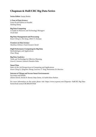
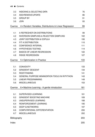
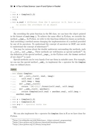
The messages displayed by invoking the interactive mode depend on both the
version of R/Python installed and the machine. Thus, you may see different messages
on your local machine. As the messages said, to quit R we can type q(). There are 3
options prompted by asking the user if the workspace should be saved or not. Since
we just want to use R as a basic calculator, we quit without saving workspace.
To quit Python, we can simply type exit().
R
1 > q()
2 Save workspace image? [y/n/c]: n
3 ~ $
Once we are inside the interactive mode, we can use R/Python as a calculator.
R
1 > 1+1
2 [1] 2
3 > 2∗3+5
4 [1] 11
5 > log(2)](https://image.slidesharecdn.com/a-tour-of-data-science-learn-r-and-python-in-parallel-1st-edition-241027161058-87cda925/85/a-tour-of-data-science-learn-r-and-python-in-parallel-1st-edition-pdf-13-320.jpg)
![Introduction to R/Python Programming • 3
6 [1] 0.6931472
7 > exp(0)
8 [1] 1
Python
1 >>> 1+1
2 2
3 >>> 2∗3+5
4 11
5 >>> log(2)
6 Traceback (most recent call last):
7 File "<stdin>", line 1, in <module >
8 NameError: name ’log’ is not defined
9 >>> exp(0)
10 Traceback (most recent call last):
11 File "<stdin>", line 1, in <module >
12 NameError: name ’exp’ is not defined
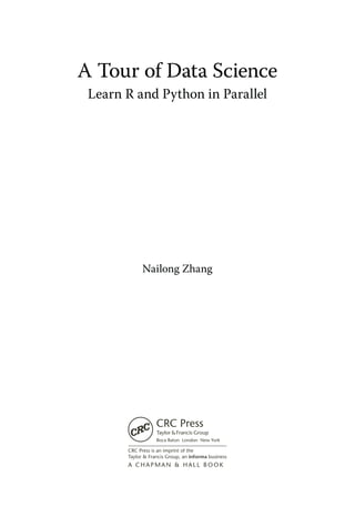
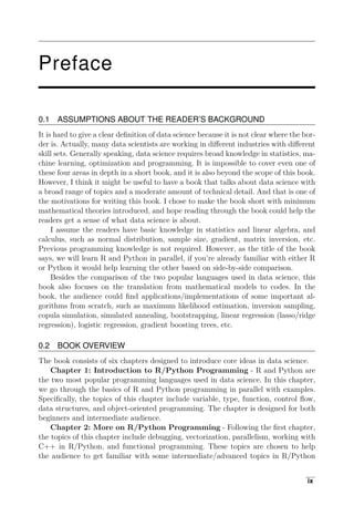
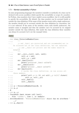
From the code snippet above, R is working as a calculator perfectly. However,
errors are raised when we call log(2) and exp(2) in Python. The error messages are
self-explanatory - log function and exp function don’t exist in the current Python
environment. In fact, log function and exp function are defined in the math module in
Python. A module3
is a file consisting of Python code. When we invoke the interactive
mode of Python, a few built-in modules are loaded into the current environment by
default. But the math module is not included in these built-in modules. That explains
why we got the NameError when we try to use the functions defined in the math
module. To resolve the issue, we should first load the functions to use by using the
import statement as follows.
Python
1 >>> from math import log, exp
2 >>> log(2)
3 0.6931471805599453
4 >>> exp(0)
5 1.0
1.2 VARIABLE AND TYPE
In the previous section we have seen how to use R/Python as calculators. Now, let’s
see how to write real programs. First, let’s define some variables.
3
https://docs.python.org/3/tutorial/modules.html](https://image.slidesharecdn.com/a-tour-of-data-science-learn-r-and-python-in-parallel-1st-edition-241027161058-87cda925/85/a-tour-of-data-science-learn-r-and-python-in-parallel-1st-edition-pdf-14-320.jpg)
![4 • A Tour of Data Science: Learn R and Python in Parallel
R Python
1 > a=2 1 >>> a=2
2 > b=5.0 2 >>> b=5.0
3 > x=’hello world’ 3 >>> x=’hello world’
4 > a 4 >>> a
5 [1] 2 5 2
6 > b 6 >>> b
7 [1] 5 7 5.0
8 > x 8 >>> x
9 [1] "hello world" 9 ’hello world’
10 > e=a∗2+b 10 >>> e=a∗2+b
11 > e 11 >>> e
12 [1] 9 12 9.0
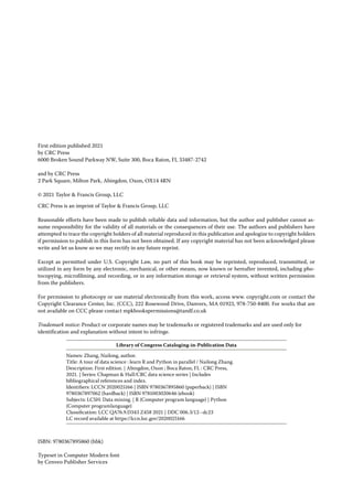
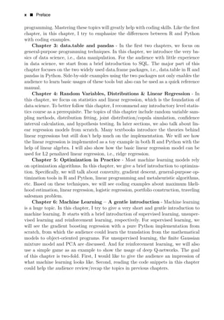
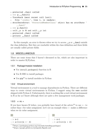
Here, we defined 4 different variables a, b, x, e. To get the type of each variable,
we can utilize the function typeof() in R and type() in Python, respectively.
R Python
1 > typeof(x) 1 >>> type(x)
2 [1] "character" 2 <class ’str’>
3 > typeof(e) 3 >>> type(e)
4 [1] "double" 4 <class ’float’>
The type of x in R is called character, and in Python is called str.
1.3 FUNCTIONS
We have seen two functions log and exp when we use R/Python as calculators.
A function is a block of code which performs a specific task. A major purpose of
wrapping a block of code into a function is to reuse the code.
It is simple to define functions in R/Python.
R Python
1 > fun1=function(x){return(x 1 >>> def fun1(x):
∗x)} 2 ... return x ote
2
∗x # n the
> fun1 indentation
3 function(x){return(x∗x)} 3 ...
4 > fun1(2) 4 >>> fun1(2)
5 [1] 4 5 4
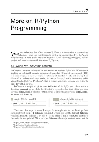
Here, we defined a function fun1 in R/Python. This function takes x as input and
returns the square of x. When we call a function, we simply type the function name](https://image.slidesharecdn.com/a-tour-of-data-science-learn-r-and-python-in-parallel-1st-edition-241027161058-87cda925/85/a-tour-of-data-science-learn-r-and-python-in-parallel-1st-edition-pdf-15-320.jpg)
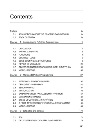
![Introduction to R/Python Programming • 5
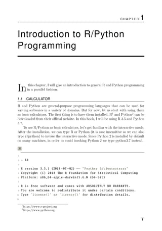
followed by the input argument inside a pair of parentheses. It is worth noting that
input or output are not required to define a function. For example, we can define a
function fun2 to print Hello World! without input and output.
One major difference between R and Python codes is that Python codes are
structured with indentation. Each logical line of R/Python code belongs to a certain
group. In R, we use {} to determine the grouping of statements. However, in Python
we use leading whitespace (spaces and tabs) at the beginning of a logical line to
compute the indentation level of the line, which is used to determine the statements’
grouping. Let’s see what happens if we remove the leading whitespace in the Python
function above.
Python
1 >>> def fun1(x):
2 ... return x∗x # note the indentation
3 File "<stdin>", line 2
4 return x∗x # note the indentation
5 ^
6 IndentationError: expected an indented block
We got an IndentationError because of missing indentation.
R Python
1 > fun2=function(){print(’ 1 >>> def fun2(): print(’Hello
Hello World!’)} World!’)
2 > fun2() 2 ...
3 [1] "Hello World!" 3 >>> fun2()
4 Hello World!
Let’s go back to fun1 and have a closer look at the return. In Python, if we
want to return something we have to use the keyword return explicitly. return in
R is a function but it is not a function in Python and that is why no parenthesis
follows return in Python. In R, return is not required even though we need to return
something from the function. Instead, we can just put the variables to return in the
last line of the function defined in R. That being said, we can define fun1 as follows.
R
1 > fun1=function(x){x∗x}
Sometimes we want to give a default value to an argument for a function, and
both R and Python allow functions to have default values.
R Python](https://image.slidesharecdn.com/a-tour-of-data-science-learn-r-and-python-in-parallel-1st-edition-241027161058-87cda925/85/a-tour-of-data-science-learn-r-and-python-in-parallel-1st-edition-pdf-16-320.jpg)
![6 • A Tour of Data Science: Learn R and Python in Parallel
1 > log_fun = 1 >>> def log_fun(x, base=2):
function(x, base=2){ 2 ...
2 + return(log(x, base)) return math.log(x, base)
3 + } 3 ...
4 > log_fun(5, base=2) 4 >>> log_fun(5,2)
5 [1] 2.321928 5 2.321928094887362
6 > log_fun(5, 2) 6 >>> log_fun(5, base=2)
7 [1] 2.321928 7 2.321928094887362
8 > log_fun(base=2, 5) 8 >>> log_fun(base=2, 5)
9 [1] 2.321928 9 File "<stdin>", line 1
10 > 10 SyntaxError: positional
argument follows keyword
argument
In Python we have to put the arguments with default values at the end, which
is not required in R. However, from a readability perspective, it is always better to
put them at the end. You may have noticed the error message above about positional
argument. In Python there are two types of arguments, i.e., positional arguments
and keyword arguments. Simply speaking, a keyword argument must be preceded
by an identifier, e.g., base in the example above. And positional arguments refer to
non-keyword arguments.
1.4 CONTROL FLOWS
To implement a complex logic in R/Python, we may need control flows.
1.4.1 If/else
Let’s define a function to return the absolute value of input.
R Python
1 > fun3=function(x){ 1 >>> def fun3(x):
2 + if (x>=0){ 2 ... if x>=0:
3 + return(x)} 3 ... return x
4 + else{ 4 ... else:
5 + return( x)}
6
− 5 ... return x
+ } 6
−
...
7 > fun3(2.5) 7 >>> fun3(2.5)
8 [1] 2.5 8 2.5
9 > fun3(−2.5) 9 >>> fun3(
10
−2.5)
[1] 2.5 10 2.5
The code snippet above shows how to use if/else in R/Python. The subtle](https://image.slidesharecdn.com/a-tour-of-data-science-learn-r-and-python-in-parallel-1st-edition-241027161058-87cda925/85/a-tour-of-data-science-learn-r-and-python-in-parallel-1st-edition-pdf-17-320.jpg)
![Introduction to R/Python Programming • 7
difference between R and Python is that the condition after if must be embraced by
parenthesis in R but it is optional in Python.
We can also put if after else. But in Python, we use elif as a shortcut.
R Python
1 > fun4=function(x){ 1 >>> def fun4(x):
2 + if (x==0){ 2 ... if x==0:
3 + print(’zero’)} 3 ... print(’zero’)
4 + else if (x>0){ 4 ... elif x>0:
5 + print(’positive’)} 5 ... print(’positive’)
6 + else{ 6 ... else:
7 + print(’negative’)} 7 ... print(’negative’)
8 + } 8 ...
9 > fun4(0) 9 >>> fun4(0)
10 [1] "zero" 10 zero
11 > fun4(1) 11 >>> fun4(1)
12 [1] "positive" 12 positive
13 > fun4(−1) 13 >>> fun4(
14
−1)
[1] "negative" 14 negative
1.4.2 For loop
Similar to the usage of if in R, we also have to use parenthesis after the keyword for
in R. But in Python there should be no parenthesis after for.
R Python
1 > for (i in 1:3){print(i)} 1 >>> for i in
range(1,4):print(i)
2 [1] 1
2
3 [1] 2
...
3 1
4 [1] 3
4 2
5 3
There is something more interesting than the for loop itself in the snippets above.
In the R code, the expression 1:3 creates a vector with elements 1, 2 and 3. In the
Python code, we use the range() function for the first time. Let’s have a look at
them.
R Python
1 > typeof(1:3) 1 >>> type(range(1,4))
2 [1] "integer" 2 <class ’range’>
range() function returns a range type object, which represents an immutable](https://image.slidesharecdn.com/a-tour-of-data-science-learn-r-and-python-in-parallel-1st-edition-241027161058-87cda925/85/a-tour-of-data-science-learn-r-and-python-in-parallel-1st-edition-pdf-18-320.jpg)
![8 • A Tour of Data Science: Learn R and Python in Parallel
sequence of numbers. range() function can take three arguments, i.e., range(start,
stop, step). However, start and step are both optional. It’s critical to keep in mind
that the stop argument that defines the upper limit of the sequence is exclusive. And
that is why in order to loop through 1 to 3 we have to pass 4 as the stop argument
to range() function. The step argument specifies how much to increase from one
number to the next. The default values of start and step are 0 and 1, respectively.
1.4.3 While loop
R Python
1 > i=1 1 >>> i=1
2 > while (i<=3){ 2 >>> while i<=3:
3 + print(i) 3 ... print(i)
4 + i=i+1 4 ... i+=1
5 + } 5 ...
6 [1] 1 6 1
7 [1] 2 7 2
8 [1] 3 8 3
You may have noticed that in Python we can do i+=1 to add 1 to i, which is not
feasible in R by default. Both for loop and while loop can be nested.
1.4.4 Break/continue
Break/continue helps if we want to break the for/while loop earlier, or to skip a
specific iteration. In R, the keyword for continue is called next, in contrast to continue
in Python. The difference between break and continue is that calling break would
exit the innermost loop (when there are nested loops, only the innermost loop is
affected); while calling continue would just skip the current iteration and continue
the loop if not finished.
R Python
1 > for (i in 1:3){ 1 >>> for i in range(1,4):
2 + print(i) 2 ... print(i)
3 + if (i==1) break 3 ... if i==1: break
4 + } 4 ...
5 [1] 1 5 1
6 > for (i in 1:3){ 6 >>> for i in range(1,4):
7 + if (i==2){next} 7 ... if i==2: continue
8 + print(i) 8 ... print(i)
9 + } 9 ...
10 [1] 1 10 1
11 [1] 3 11 3](https://image.slidesharecdn.com/a-tour-of-data-science-learn-r-and-python-in-parallel-1st-edition-241027161058-87cda925/85/a-tour-of-data-science-learn-r-and-python-in-parallel-1st-edition-pdf-19-320.jpg)
![Introduction to R/Python Programming • 9
1.5 SOME BUILT-IN DATA STRUCTURES
In the previous sections, we haven’t seen much difference between R and Python.
However, regarding the built-in data structures, there are some significant differences
we will see in this section.
1.5.1 Vector in R and list in Python
In R, we can use function c() to create a vector; A vector is a sequence of elements
with the same type. In Python, we can use [] to create a list, which is also a sequence
of elements. But the elements in a list don’t need to have the same type. To get the
number of elements in a vector in R, we use the function length(); and to get the
number of elements in a list in Python, we use the function len().
R Python
1 > x=c(1,2,5,6) 1 >>> x=[1,2,5,6]
2 > y=c(’hello’,’world’,’!’) 2 >>> y=[’hello’,’world’,’!’]
3 > x 3 >>> x
4 [1] 1 2 5 6 4 [1, 2, 5, 6]
5 > y 5 >>> y
6 [1] "hello" "world" "!" 6 [’hello’, ’world’, ’!’]
7 > length(x) 7 >>> len(x)
8 [1] 4 8 4
9 > z=c(1,’hello’) 9 >>> z=[1,’hello’]
10 > z 10 >>> z
11 [1] "1" "hello" 11 [1, ’hello’]
In the code snippet above, the first element in the variable z in R is coerced from
1 (numeric) to "1" (character) since the elements must have the same type.
To access a specific element from a vector or list, we could use []. In R, sequence
types are indexed beginning with the one subscript. In contrast, sequence types in
Python are indexed beginning with the zero subscript.
R Python
1 > x=c(1,2,5,6) 1 >>> x=[1,2,5,6]
2 > x[1] 2 >>> x[1]
3 [1] 1 3 2
4 >>> x[0]
5 1
What if the index to access is out of boundary?](https://image.slidesharecdn.com/a-tour-of-data-science-learn-r-and-python-in-parallel-1st-edition-241027161058-87cda925/85/a-tour-of-data-science-learn-r-and-python-in-parallel-1st-edition-pdf-20-320.jpg)
![10 • A Tour of Data Science: Learn R and Python in Parallel
R Python
1 > x=c(1,2,5,6) 1 >>> x=[1,2,5,6]
2 > x[−1] 2 >>> x[−1]
3 [1] 2 5 6 3 6
4 > x[0] 4 >>> x[len(x)+1]
5 numeric(0) 5 Traceback (most recent call
6 > x[length(x)+1] last):
7 [1] NA 6 File "<stdin>", line 1,
in <module >
8 > length(numeric(0))
7 IndexError:
9 [1] 0 list index out of range
10 > length(NA)
11 [1] 1
In Python, negative index number means indexing from the end of the list. Thus,
x[−1] points to the last element and x[−2] points to the second-last element of
the list. But R doesn’t support indexing with negative numbers in the same way as
Python. Specifically, in R x[−index] returns a new vector with x[index] excluded.
When we try to access with an index out of boundary, Python would throw an
IndexError. The behavior of R when indexing out of boundary is more interesting.
First, when we try to access x[0] in R we get a numeric(0) whose length is also
0. Since its length is 0, numeric(0) can be interpreted as an empty numeric vector.
When we try to access x[length(x)+1] we get an NA. In R, there are also NaN and
NULL.
NaN means "Not A Number" and it can be verified by checking its type - "double".
0/0 would result in an NaN in R. NA in R generally represents missing values. And
NULL represents a NULL (empty) object. To check if a value is NA, NaN or NULL, we
can use is.na(), is.nan() or is.null, respectively.
R Python
1 > typeof(NA) 1 >>> type(None)
2 [1] "logical" 2 <class ’NoneType’>
3 > typeof(NaN) 3 >>> None is None
4 [1] "double" 4 True
5 > typeof(NULL) 5 >>> 1 == None
6 [1] "NULL" 6 False
7 > is.na(NA)
8 [1] TRUE
9 > is.null(NULL)
10 [1] TRUE
11 > is.nan(NaN)
In Python, there is no built-in NA or NaN. The counterpart of NULL in Python is](https://image.slidesharecdn.com/a-tour-of-data-science-learn-r-and-python-in-parallel-1st-edition-241027161058-87cda925/85/a-tour-of-data-science-learn-r-and-python-in-parallel-1st-edition-pdf-21-320.jpg)
![Introduction to R/Python Programming • 11
None. In Python, we can use the is keyword or == to check if a value is equal to
None.
From the code snippet above, we also notice that in R the boolean type value
is written as "TRUE/FALSE", compared with "True/False" in Python. Although in
R "TRUE/FALSE" can also be abbreviated as "T/F", I don’t recommend using the
abbreviation.
There is one interesting fact that we can’t add a NULL to a vector in R, but it is
feasible to add a None to a list in Python.
R Python
1 > x=c(1,NA,NaN,NULL) 1 >>> x=[1,None]
2 > x 2 >>> x
3 [1] 1 NA NaN 3 [1, None]
4 > length(x) 4 >>> len(x)
5 [1] 3 5 2
Sometimes we want to create a vector/list with replicated elements, for example,
a vector/list with all elements equal to 0.
R Python
1 > x=rep(0, 10) 1 >>> x=[0]
2
∗10
> x 2 >>> x
3 [1] 0 0 0 0 0 0 0 0 0 0 3 [0, 0, 0, 0, 0, 0, 0, 0, 0,
4 > y=rep(c(0,1), 5) 0]
5 > y 4 >>> y=[0, 1]∗5
6 [1] 0 1 0 1 0 1 0 1 0 1 5 >>> y
6 [0, 1, 0, 1, 0, 1, 0, 1, 0,
1]
When we use the ∗ operator to make replicates of a list, there is one caveat - if
the element inside the list is mutable then the replicated elements point to the same
memory address. As a consequence, if one element is mutated other elements are also
affected.
Python
1 >>> x=[0] # x is a list which is mutable
2 >>> y=[x]∗5 # each element in y points to x
3 >>> y
4 [[0], [0], [0], [0], [0]]
5 >>> y[2]=2 # we point y[2] to 2 but x is not mutated
6 >>> y
7 [[0], [0], 2, [0], [0]]
8 >>> y[1][0]=−1 # we mutate x by changing y[1][0] from 0 to −1](https://image.slidesharecdn.com/a-tour-of-data-science-learn-r-and-python-in-parallel-1st-edition-241027161058-87cda925/85/a-tour-of-data-science-learn-r-and-python-in-parallel-1st-edition-pdf-22-320.jpg)
![12 • A Tour of Data Science: Learn R and Python in Parallel
9 >>> y
10 [[−1], [−1], 2, [−1], [−1]]
11 >>> x
12 [−1]
How to get a list with replicated elements but pointing to different memory ad
dresses?
Python
1 >>> x=[0]
2 >>> y=[x[:] for _ in range(5)] # [:] makes a copy of the list x;
another solution is [list(x) for _ in range(5)]
3 >>> y
4 [[0], [0], [0], [0], [0]]
5 >>> y[0][0]=2
6 >>> y
7 [[2], [0], [0], [0], [0]]
Besides accessing a specific element from a vector/list, we may also need to do
slicing, i.e., to select a subset of the vector/list. There are two basic approaches of
slicing:
• Integer-based
R
1 > x=c(1,2,3,4,5,6)
2 > x[2:4]
3 [1] 2 3 4
4 > x[c(1,2,5)] # a vector of indices
5 [1] 1 2 5
6 > x[seq(1,5,2)] # seq creates a vector to be used as
indices
7 [1] 1 3 5
Python
1 >>> x=[1,2,3,4,5,6]
2 >>> x[1:4] # x[start:end] start is inclusive but end is
exclusive
3 [2, 3, 4]
4 >>> x[0:5:2] # x[start:end:step]
5 [1, 3, 5]](https://image.slidesharecdn.com/a-tour-of-data-science-learn-r-and-python-in-parallel-1st-edition-241027161058-87cda925/85/a-tour-of-data-science-learn-r-and-python-in-parallel-1st-edition-pdf-23-320.jpg)
![Introduction to R/Python Programming • 13
The code snippet above uses hash character # for comments in both R and
Python. Everything after # on the same line would be treated as comment (not
executable). In the R code, we also used the function seq() to create a vector.
When I see a function that I haven’t seen before, I might either google it or
use the built-in helper mechanism. Specifically, in R use ? and in Python use
help().
R Python
1 > ?seq 1 >>> help(print)
• Condition-based
Condition-based slicing means to select a subset of the elements which satisfy
certain conditions. In R, it is quite straightforward by using a boolean vector
whose length is the same as the vector to be sliced.
R
1 > x=c(1,2,5,5,6,6)
2 > x[x %% 2==1] # %% is the modulo operator in R; we select
the odd elements
3 [1] 1 5 5
4 > x %% 2==1 # results in a boolean vector with the same
length as x
5 [1] TRUE FALSE TRUE TRUE FALSE FALSE
The condition-based slicing in Python is quite different from that in R. The
prerequisite is list comprehension which provides a concise way to create new
lists in Python. For example, let’s create a list of squares of another list.
Python
1 >>> x=[1,2,5,5,6,6]
2 >>> [e∗∗2 for e in x] # ∗∗ is the exponent operator , i.e.,
x∗∗y means x to the power of y
3 [1, 4, 25, 25, 36, 36]
We can also use if statement with list comprehension to filter a list to achieve
list slicing.
Python](https://image.slidesharecdn.com/a-tour-of-data-science-learn-r-and-python-in-parallel-1st-edition-241027161058-87cda925/85/a-tour-of-data-science-learn-r-and-python-in-parallel-1st-edition-pdf-24-320.jpg)
![14 • A Tour of Data Science: Learn R and Python in Parallel
1 >>> x=[1,2,5,5,6,6]
2 >>> [e for e in x if e%2==1] # % is the modulo operator in
Python
3 [1, 5, 5]
It is also common to use if/else with list comprehension to achieve more
complex operations. For example, given a list x, let’s create a new list y so
that the non-negative elements in x are squared and the negative elements are
replaced by 0s.
Python
1 >>> x=[1,−1,0,2,5,−3]
2 >>> [e∗∗2 if e>=0 else 0 for e in x]
3 [1, 0, 0, 4, 25, 0]
The example above shows the power of list comprehension. To use if with list
comprehension, the if statement should be placed in the end after the for loop
statement; but to use if/else with list comprehension, the if/else statement
should be placed before the for loop statement.
We can also modify the value of an element in a vector/list variable.
R Python
1 > x=c(1,2,3) 1 >>> x=[1,2,3]
2 > x[1]= 1 2 >>> x[0]= 1
3
− −
> x 3 >>> x
4 [1] −1 2 3 4 [−1, 2, 3]
Two or multiple vectors/lists can be concatenated easily.
R Python
1 > x=c(1,2) 1 >>> x=[1,2]
2 > y=c(3,4) 2 >>> y=[3,4]
3 > z=c(5,6,7,8) 3 >>> z=[5,6,7,8]
4 > c(x,y,z) 4 >>> x+y+z
5 [1] 1 2 3 4 5 6 7 8 5 [1, 2, 3, 4, 5, 6, 7, 8]
As the list structure in Python is mutable, there are many things we can do with
list.](https://image.slidesharecdn.com/a-tour-of-data-science-learn-r-and-python-in-parallel-1st-edition-241027161058-87cda925/85/a-tour-of-data-science-learn-r-and-python-in-parallel-1st-edition-pdf-25-320.jpg)
![Introduction to R/Python Programming • 15
Python
1 >>> x=[1,2,3]
2 >>> x.append(4) # append a single value to the list x
3 >>> x
4 [1, 2, 3, 4]
5 >>> y=[5,6]
6 >>> x.extend(y) # extend list y to x
7 >>> x
8 [1, 2, 3, 4, 5, 6]
9 >>> last=x.pop() # pop the last element from x
10 >>> last
11 6
12 >>> x
13 [1, 2, 3, 4, 5]
I like the list structure in Python much more than the vector structure in R. list
in Python has a lot more useful features which can be found from the python official
documentation4
.
1.5.2 Array
Array is one of the most important data structures in scientific programming. In R,
there is also an object type "matrix", but according to my own experience, we can
almost ignore its existence and use array instead. We can definitely use list as array
in Python, but lots of linear algebra operations are not supported for the list type.
Fortunately, there is a Python package numpy off the shelf.
R
1 > x=1:12
2 > array1=array(x, c(4,3)) # convert vector x to a 4 rows ∗ 3
cols array
3 > array1
4 [,1] [,2] [,3]
5 [1,] 1 5 9
6 [2,] 2 6 10
7 [3,] 3 7 11
8 [4,] 4 8 12
9 > y=1:6
10 > array2=array(y, c(3,2)) # convert vector y to a 3 rows ∗ 2
cols array
11 > array2
12 [,1] [,2]
4
https://docs.python.org/3/tutorial/datastructures.html](https://image.slidesharecdn.com/a-tour-of-data-science-learn-r-and-python-in-parallel-1st-edition-241027161058-87cda925/85/a-tour-of-data-science-learn-r-and-python-in-parallel-1st-edition-pdf-26-320.jpg)
![16 • A Tour of Data Science: Learn R and Python in Parallel
13 [1,] 1 4
14 [2,] 2 5
15 [3,] 3 6
16 > array3 = array1 %∗% array2 # %∗% is the matrix multiplication
operator
17 > array3
18 [,1] [,2]
19 [1,] 38 83
20 [2,] 44 98
21 [3,] 50 113
22 [4,] 56 128
23 > dim(array3) # get the dimension of array3
24 [1] 4 2
Python
1 >>> import numpy as np # we import the numpy module and alias it
as np
2 >>> array1=np.reshape(list(range(1,13)),(4,3)) # convert a list
to a 2d np.array
3 >>> array1
4 array([[ 1, 2, 3],
5 [ 4, 5, 6],
6 [ 7, 8, 9],
7 [10, 11, 12]])
8 >>> type(array1)
9 <class ’numpy.ndarray’>
10 >>> array2=np.reshape(list(range(1,7)),(3,2))
11 >>> array2
12 array([[1, 2],
13 [3, 4],
14 [5, 6]])
15 >>> array3=np.dot(array1, array2) # matrix multiplication using
np.dot()
16 >>> array3
17 array([[ 22, 28],
18 [ 49, 64],
19 [ 76, 100],
20 [103, 136]])
21 >>> array3.shape # get the shape(dimension) of array3
22 (4, 2)
You may have noticed that the results of the R code snippet and Python code
snippet are different. The reason is that in R the conversion from a vector to an array](https://image.slidesharecdn.com/a-tour-of-data-science-learn-r-and-python-in-parallel-1st-edition-241027161058-87cda925/85/a-tour-of-data-science-learn-r-and-python-in-parallel-1st-edition-pdf-27-320.jpg)
![Introduction to R/Python Programming • 17
is by-column; but in numpy the reshape from a list to a 2D numpy.array is by-row.
There are two ways to reshape a list to a 2D numpy.array by column.
Python
1 >>> array1=np.reshape(list(range(1,13)),(4,3),order=’F’) # use
order=’F’
2 >>> array1
3 array([[ 1, 5, 9],
4 [ 2, 6, 10],
5 [ 3, 7, 11],
6 [ 4, 8, 12]])
7 >>> array2=np.reshape(list(range(1,7)),(2,3)).T # use .T to
transpose an array
8 >>> array2
9 array([[1, 4],
10 [2, 5],
11 [3, 6]])
12 >>> np.dot(array1 , array2) # now we get the same result as using
R
13 array([[ 38, 83],
14 [ 44, 98],
15 [ 50, 113],
16 [ 56, 128]])
To learn more about numpy, the official website5
has great documentation/tutori
als.
The term broadcasting describes how arrays with different shapes are handled
during arithmetic operations. A simple example of broadcasting is given below.
R Python
1 > x = c(1, 2, 3) 1 >>> import numpy as np
2 > x+1 2 >>> x = np.array([1, 2, 3])
3 [1] 2 3 4 3 >>> x + 1
4 array([2, 3, 4])
However, the broadcasting rules in R and Python are not exactly the same.
R Python
1 > x = array(c(1:6), c(3,2)) 1 >>> import numpy as np
2 > y = c(1, 2, 3) 2 >>> x = np.array([[1, 2],
3 > z = c(1, 2) [3, 4], [5, 6]])
5
http://www.numpy.org](https://image.slidesharecdn.com/a-tour-of-data-science-learn-r-and-python-in-parallel-1st-edition-241027161058-87cda925/85/a-tour-of-data-science-learn-r-and-python-in-parallel-1st-edition-pdf-28-320.jpg)
![18 • A Tour of Data Science: Learn R and Python in Parallel
4 # point−wise multiplication 3 >>> y = np.array([1, 2, 3])
5 > x ∗ y 4 >>> z = np.array([1, 2])
6 [,1] [,2] 5 >>> # point−wise
multiplication
7 [1,] 1 4
6 >>> x y
8 [2,] 4 10
7
∗
Traceback (most recent call
9 [3,] 9 18
last):
10 > x∗z
8 File "<stdin>", line 1,
11 [,1] [,2] in <module >
12 [1,] 1 8 9 ValueError: operands could
13 not
[2,] 4 5 be broadcast together
with shapes (3,2) (3,)
14 [3,] 3 12
10 >>> x ∗ z
11 array([[ 1, 4],
12 [ 3, 8],
13 [ 5, 12]])
From the R code, we see the broadcasting in R is like recycling along with the
column. In Python, when the two arrays have different dimensions, the one with fewer
dimensions is padded with ones on its leading side. According to this rule, when we
do x ∗ y, the dimension of x is (3, 2) but the dimension of y is 3. Thus, the dimension
of y is padded to (1, 3), which explains what happens when x ∗ y.
1.5.3 List in R and dictionary in Python
Yes, in R there is also an object type called list. The major difference between a
vector and a list in R is that a list could contain different types of elements. list in R
supports integer-based accessing using [[]] (compared to [] for vector).
R
1 > x=list(1,’hello world!’)
2 > x
3 [[1]]
4 [1] 1
5
6 [[2]]
7 [1] "hello world!"
8
9 > x[[1]]
10 [1] 1
11 > x[[2]]
12 [1] "hello world!"
13 > length(x)
14 [1] 2](https://image.slidesharecdn.com/a-tour-of-data-science-learn-r-and-python-in-parallel-1st-edition-241027161058-87cda925/85/a-tour-of-data-science-learn-r-and-python-in-parallel-1st-edition-pdf-29-320.jpg)
![Introduction to R/Python Programming • 19
list in R could be named and support accessing by name via either [[]] or $
operator. But vector in R can also be named and support accessing by name.
R
1 > x=c(’a’=1,’b’=2)
2 > names(x)
3 [1] "a" "b"
4 > x[’b’]
5 b
6 2
7 > l=list(’a’=1,’b’=2)
8 > l[[’b’]]
9 [1] 2
10 > l$b
11 [1] 2
12 > names(l)
13 [1] "a" "b"
However, elements in list in Python can’t be named as R. If we need the feature
of accessing by name in Python, we can use the dictionary structure. If you used
Java before, you may consider dictionary in Python as the counterpart of HashMap
in Java. Essentially, a dictionary in Python is a collection of key:value pairs.
Python
1 >>> x={’a’:1,’b’:2} # {key:value} pairs
2 >>> x
3 {’a’: 1, ’b’: 2}
4 >>> x[’a’]
5 1
6 >>> x[’b’]
7 2
8 >>> len(x) # number of key:value pairs
9 2
10 >>> x.pop(’a’) # remove the key ’a’ and we get its value 1
11 1
12 >>> x
13 {’b’: 2}
Unlike dictionary in Python, list in R doesn’t support the pop() operation. Thus,
in order to modify a list in R, a new one must be created explicitly or implicitly.](https://image.slidesharecdn.com/a-tour-of-data-science-learn-r-and-python-in-parallel-1st-edition-241027161058-87cda925/85/a-tour-of-data-science-learn-r-and-python-in-parallel-1st-edition-pdf-30-320.jpg)
![20 • A Tour of Data Science: Learn R and Python in Parallel
1.5.4 data.frame, data.table and pandas
data.frame is a built-in type in R for data manipulation. In Python, there is no
such built-in data structure since Python is a more general-purpose programming
language. The solution for data.frame in Python is the pandas6
module.
Before we dive into data.frame, you may be curious as to why we need it. In other
words, why can’t we just use vector, list, array/matrix and dictionary for all data
manipulation tasks? I would say yes - data.frame is not a must-have feature for most
of ETL (extraction, transformation and Load) operations. But data.frame provides a
very intuitive way for us to understand the structured dataset. A data.frame is usually
flat with 2 dimensions, i.e., row and column. The row dimension is across multiple
observations and the column dimension is across multiple attributes/features. If you
are familiar with relational database, a data.frame can be viewed as a table.
Let’s see an example of using data.frame to represent employees’ information in
a company.
R
1 > employee_df = data.
frame(name=c("A", "B", "C
"),department=c("
Engineering","Operations
","Sales"))
2 > employee_df
3 name department
4 1 A Engineering
5 2 B Operations
6 3 C Sales
Python
1 >>> import pandas as pd
2 >>> employee_df=pd.DataFrame
({’name’:[’A’,’B’,’C’],’
department’:["Engineering
","Operations","Sales"]})
3 >>> employee_df
4 name department
5 0 A Engineering
6 1 B Operations
7 2 C Sales
There are quite a few ways to create data.frame. The most commonly used one
is to create data.frame object from array/matrix. We may also need to convert a
numeric data.frame to an array/matrix.
R
1 > x=array(rnorm(12), c(3,4))
2 > x
3 [,1] [,2] [,3] [,4]
4 [1,] −0.8101246 −0.8594136 −2.260810 0.5727590
5 [2,] −0.9175476 0.1345982 1.067628 −0.7643533
6 [3,] 0.7865971 −1.9046711 −0.154928 −0.6807527
7 > random_df=as.data.frame(x)
8 > random_df
9 V1 V2 V3 V4
10 1 −0.8101246 −0.8594136 −2.260810 0.5727590
6
https://pandas.pydata.org/](https://image.slidesharecdn.com/a-tour-of-data-science-learn-r-and-python-in-parallel-1st-edition-241027161058-87cda925/85/a-tour-of-data-science-learn-r-and-python-in-parallel-1st-edition-pdf-31-320.jpg)
![Introduction to R/Python Programming • 21
11 2 −0.9175476 0.1345982 1.067628 −0.7643533
12 3 0.7865971 −1.9046711 −0.154928 −0.6807527
13 > data.matrix(random_df)
14 V1 V2 V3 V4
15 [1,] −0.8101246 −0.8594136 −2.260810 0.5727590
16 [2,] −0.9175476 0.1345982 1.067628 −0.7643533
17 [3,] 0.7865971 −1.9046711 −0.154928 −0.6807527
Python
1 >>> import numpy as np
2 >>> import pandas as pd
3 >>> x=np.random.normal(size=(3,4))
4 >>> x
5 array([[−0.54164878, −0.14285267, −0.39835535, −0.81522719],
6 [ 0.01540508, 0.63556266, 0.16800583, 0.17594448],
7 [−1.21598262, 0.52860817, −0.61757696, 0.18445057]])
8 >>> random_df = pd.DataFrame(x)
9 >>> random_df
10 0 1 2 3
11 0 −0.541649 −0.142853 −0.398355 −0.815227
12 1 0.015405 0.635563 0.168006 0.175944
13 2 −1.215983 0.528608 −0.617577 0.184451
14 >>> np.asarray(random_df)
15 array([[−0.54164878, −0.14285267, −0.39835535, −0.81522719],
16 [ 0.01540508, 0.63556266, 0.16800583, 0.17594448],
17 [−1.21598262, 0.52860817, −0.61757696, 0.18445057]])
In general, operations on an array/matrix are much faster than those on a data
frame. In R, we may use the built-in function data.matrix to convert a data.frame
to an array/matrix. In Python, we could use the function asarray in numpy module.
Although data.frame is a built-in type, it is not quite efficient for many operations.
I would suggest using data.table7
whenever possible. 8
dplyr is also a very popular
package in R for data manipulation. Many good resources are available online to
learn data.table and pandas.
1.6 REVISIT OF VARIABLES
We have talked about variables and functions so far. When a function has a name,
its name is also a valid variable. After all, what is a variable?
In mathematics, a variable is a symbol that represents an element, and we do
7
https://cran.r-project.org/web/packages/data.table/index.html
8
https://dplyr.tidyverse.org/](https://image.slidesharecdn.com/a-tour-of-data-science-learn-r-and-python-in-parallel-1st-edition-241027161058-87cda925/85/a-tour-of-data-science-learn-r-and-python-in-parallel-1st-edition-pdf-32-320.jpg)
![22 • A Tour of Data Science: Learn R and Python in Parallel
not care whether we conceptualize a variable in our mind, or write it down on paper.
However, in programming a variable is not only a symbol. We have to understand
that a variable is a name given to a memory location in computer systems. When we
run x = 2 in R or Python, somewhere in memory has the value 2, and the variable
(name) points to this memory address. If we further run y = x, the variable y points
to the same memory location pointed to by (x). What if we run x=3? It doesn’t
modify the memory which stores the value 2. Instead, somewhere in the memory now
has the value 3 and this memory location has a name x. And the variable y is not
affected at all, as well as the memory location it points to.
1.6.1 Mutability
Almost everything in R or Python is an object, including these data structures we
introduced in previous sections. Mutability is a property of objects, not variables,
because a variable is just a name.
A list in Python is mutable, meaning that we could change the elements stored in
the list object without copying the list object from one memory location to another.
We can use the id function in Python to check the memory location for a variable.
In the code below, we modified the first element of the list object with name x. And
since Python list is mutable, the memory address of the list doesn’t change.
Python
1 >>> x=list(range(1,1001)) # list() convert a range object to a
list
2 >>> hex(id(x)) # print the memory address of x
3 ’0x10592d908’
4 >>> x[0]=1.0 # from integer to float
5 >>> hex(id(x))
6 ’0x10592d908’
Is there any immutable data structure in Python? Yes, for example tuple is im
mutable, which contains a sequence of elements. The element accessing and subset
slicing of tuple follows the same rules as list in Python.
Python
1 >>> x=(1,2,3,) # use () to create a tuple in Python, it is
better to always put a comma in the end
2 >>> type(x)
3 <class ’tuple’>
4 >>> len(x)
5 3
6 >>> x[0]
7 1
8 >>> x[0]=−1](https://image.slidesharecdn.com/a-tour-of-data-science-learn-r-and-python-in-parallel-1st-edition-241027161058-87cda925/85/a-tour-of-data-science-learn-r-and-python-in-parallel-1st-edition-pdf-33-320.jpg)
![Introduction to R/Python Programming • 23
9 Traceback (most recent call last):
10 File "<stdin>", line 1, in <module >
11 TypeError: ’tuple’ object does not support item assignment
If we have two Python variables pointed to the same memory, when we modify
the memory via one variable the other is also affected as we expect (see the example
below).
Python
1 >>> x=[1,2,3]
2 >>> id(x)
3 4535423616
4 >>> x[0]=0
5 >>> x=[1,2,3]
6 >>> y=x
7 >>> id(x)
8 4535459104
9 >>> id(y)
10 4535459104
11 >>> x[0]=0
12 >>> id(x)
13 4535459104
14 >>> id(y)
15 4535459104
16 >>> x
17 [0, 2, 3]
18 >>> y
19 [0, 2, 3]
In contrast, the mutability of vector in R is more complex and sometimes con
fusing. First, let’s see the behavior when there is a single name given to the vector
object stored in memory.
R
1 > a=c(1,2,3)
2 > .Internal(inspect(a))
3 @7fe94408f3c8 14 REALSXP g0c3 [NAM(1)] (len=3, tl=0) 1,2,3
4 > a[1]=0
5 > .Internal(inspect(a))
6 @7fe94408f3c8 14 REALSXP g0c3 [NAM(1)] (len=3, tl=0) 0,2,3
It is clear in this case the vector object is mutable since the memory address](https://image.slidesharecdn.com/a-tour-of-data-science-learn-r-and-python-in-parallel-1st-edition-241027161058-87cda925/85/a-tour-of-data-science-learn-r-and-python-in-parallel-1st-edition-pdf-34-320.jpg)
![24 • A Tour of Data Science: Learn R and Python in Parallel
doesn’t change after the modification. What if there is an additional name given to
the memory?
R
1 > a=c(1,2,3)
2 > b=a
3 > .Internal(inspect(a))
4 @7fe94408f238 14 REALSXP g0c3 [NAM(2)] (len=3, tl=0) 1,2,3
5 > .Internal(inspect(b))
6 @7fe94408f238 14 REALSXP g0c3 [NAM(2)] (len=3, tl=0) 1,2,3
7 > a[1]=0
8 > .Internal(inspect(a))
9 @7fe94408f0a8 14 REALSXP g0c3 [NAM(1)] (len=3, tl=0) 0,2,3
10 > .Internal(inspect(b))
11 @7fe94408f238 14 REALSXP g0c3 [NAM(2)] (len=3, tl=0) 1,2,3
12 > a
13 [1] 0 2 3
14 > b
15 [1] 1 2 3
Before the modification, both variable a and b point to the same vector object in
the memory. But surprisingly, after the modification the memory address of variable
a also changed, which is called "copy on modify" in R. And because of this unique
behavior, the modification of a doesn’t affect the object stored in the old memory
and thus the vector object is immutable in this case. The mutability of R list is
similar to that of R vector.
1.6.2 Variable as function argument
Most functions/methods in R and Python take some variables as argument. What
happens when we pass the variables into a function?
In Python, the variable, i.e., the name of the object, is passed into a function. If
the variable points to an immutable object, any modification to the variable, i.e., the
name, doesn’t persist. However, when the variable points to a mutable object, the
modification of the object stored in memory persists. Let’s see the examples below.
Python Python
1 >>> def g(x): 1 >>> def f(x):
2 ... print(id(x)) 2 ... id(x)
3 ... x−=1 3 ... x[0] =1
−
4 ... print(id(x)) 4 ... id(x)
5 ... print(x) 5 >>> a=[1,2,3]
6 >>> a=1 6 >>> id(a)
7 >>> id(a) 7 4535423616](https://image.slidesharecdn.com/a-tour-of-data-science-learn-r-and-python-in-parallel-1st-edition-241027161058-87cda925/85/a-tour-of-data-science-learn-r-and-python-in-parallel-1st-edition-pdf-35-320.jpg)
![Introduction to R/Python Programming • 25
8 4531658512 8 >>> f(a)
9 >>> g(a) 9 4535423616
10 4531658512 10 4535423616
11 4531658480 11 >>> a
12 0 12 [0, 2, 3]
13 >>> a
14 1
We see that the object is passed into function by its name. If the object is im
mutable, a new copy is created in memory when any modification is made to the
original object. When the object is immutable, no new copy is made and thus the
change persists out of the function.
In R, the passed object is always copied on a modification inside the function,
and thus no modification can be made to the original object in memory.
R
1 > f=function(x){
2 + print(.Internal(inspect(x)))
3 + x[1]=x[1] 1
4
−
+ print(.Internal(inspect(x)))
5 + print(x)
6 + }
7 >
8 > a=c(1,2,3)
9 > .Internal(inspect(a))
10 @7fe945538688 14 REALSXP g0c3 [NAM(1)] (len=3, tl=0) 1,2,3
11 > f(a)
12 @7fe945538688 14 REALSXP g0c3 [NAM(3)] (len=3, tl=0) 1,2,3
13 [1] 1 2 3
14 @7fe945538598 14 REALSXP g0c3 [NAM(1)] (len=3, tl=0) 0,2,3
15 [1] 0 2 3
16 [1] 0 2 3
17 > a
18 [1] 1 2 3
People may argue that R functions are not as flexible as Python functions. How
ever, it makes more sense to do functional programming in R since we usually can’t
modify objects passed into a function.
1.6.3 Scope of variables
What is the scope of a variable and why does it matter? Let’s first have a look at the
code snippets below.](https://image.slidesharecdn.com/a-tour-of-data-science-learn-r-and-python-in-parallel-1st-edition-241027161058-87cda925/85/a-tour-of-data-science-learn-r-and-python-in-parallel-1st-edition-pdf-36-320.jpg)
![26 • A Tour of Data Science: Learn R and Python in Parallel
R Python
1 > x=1 1 >>> x=1
2 > var_func_1 = 2 >>>
function(){print(x)} def var_func_1():print(x)
3 > var_func_1() 3 >>> var_func_1()
4 [1] 1 4 1
5 > var_func_2 = function(){x= 5 >>> def var_func_2():x+=1
x+1; print(x)} 6 ...
6 > var_func_2() 7 >>> var_func_2()
7 [1] 2 8 Traceback (most recent call
8 > x last):
9 [1] 1 9 File "<stdin>", line 1,
in <module >
10 File "<stdin>", line 1,
in var_func_2
11 UnboundLocalError: local
variable ’x
’ referenced before
assignment
The results of the code above seem strange before knowing the concept of variable
scope. Inside a function, a variable may refer to a function argument/parameter or
it could be formally declared inside the function which is called a local variable. But
in the code above, x is neither a function argument nor a local variable. How does
the print() function know what the identifier x points to?
The scope of a variable determines where the variable is available/accessible (can
be referenced). Both R and Python apply lexical/static scoping for variables, which
set the scope of a variable based on the structure of the program. In static scoping,
when an ’unknown’ variable is referenced, the function will try to find it from the
most closely enclosing block. That explains how the print() function could find the
variable x.
In the R code above, x=x+1 the first x is a local variable created by the = operator;
the second x is referenced inside the function so the static scoping rule applies. As
a result, a local variable x which is equal to 2 is created, which is independent with
the x outside of the function var_func_2(). However, in Python when a variable is
assigned a value in a statement, the variable would be treated as a local variable and
that explains the UnboundLocalError.
Is it possible to change a variable inside a function which is declared outside the
function without passing it as an argument? Based on the static scoping rule only,
it’s impossible. But there are workarounds in both R/Python. In R, we need the help
of environment; and in Python we can use the keyword global.
So what is an environment in R? An environment is a place where objects are
stored. When we invoke the interactive R session, an environment named .GlobalEnv
is created automatically. We can also use the function environment() to get the](https://image.slidesharecdn.com/a-tour-of-data-science-learn-r-and-python-in-parallel-1st-edition-241027161058-87cda925/85/a-tour-of-data-science-learn-r-and-python-in-parallel-1st-edition-pdf-37-320.jpg)
![Introduction to R/Python Programming • 27
present environment. The ls() function can take an environment as the argument to
list all objects inside the environment.
R
1 $r
2 > typeof(.GlobalEnv)
3 [1] "environment"
4 > environment()
5 <environment: R_GlobalEnv >
6 > x=1
7 > ls(environment())
8 [1] "x"
9 > env_func_1=function(x){
10 + y=x+1
11 + print(environment())
12 + ls(environment())
13 + }
14 > env_func_1(2)
15 <environment: 0x7fc59d165a20 >
16 [1] "x" "y"
17 > env_func_2=function(){print(environment())}
18 > env_func_2()
19 <environment: 0x7fc59d16f520 >
The above code shows that each function has its own environment containing
all function arguments and local variables declared inside the function. In order to
change a variable declared outside of a function, we need the access of the environment
enclosing the variable to change. There is a function parent_env(e) that returns the
parent environment of the given environment e in R. Using this function, we are
able to change the value of x declared in .GlobalEnv inside a function which is also
declared in .GlobalEnv. The global keyword in Python works in a totally different
way, which is simple but less flexible.
R Python
1 > x=1 1 >>> def env_func_3():
2 > env_func_3=function(){ 2 ... global x
3 + cur_env=environment() 3 ... x = 2
4 + par_env= 4 ...
parent.env(cur_env) 5 >>> x=1
5 + par_env$x=2
6 >>> env_func_3()
6 + }
7 >>> x
7 > env_func_3()
8 2
8 > x
9 [1] 2](https://image.slidesharecdn.com/a-tour-of-data-science-learn-r-and-python-in-parallel-1st-edition-241027161058-87cda925/85/a-tour-of-data-science-learn-r-and-python-in-parallel-1st-edition-pdf-38-320.jpg)
![28 • A Tour of Data Science: Learn R and Python in Parallel
I seldom use the global keyword in Python, if ever. But the environment in R
could be very handy on some occasions. In R, environment could be used as a purely
mutable version of the list data structure. Let’s use the R function tracemem to trace
the copy of an object. It is worth nothing that tracemem can’t trace R functions.
R R
1 # list is not purely mutable 1 # environment is purely
2 > x=list(1) mutable
2 > x=new.env()
3 > tracemem(x)
3 > x
4 [1] "<0x7f829183f6f8 >"
4 <environment: 0x7f8290aee7e8
5 > x$a=2
>
6 > tracemem(x)
5 > x$a=2
7 [1] "<0x7f828f4d05c8 >"
6 > x
7 <environment: 0x7f8290aee7e8
>
Actually, the object of an R6 class type is also an environment.
R
1 > # load the Complex class that we defined in chapter 1
2 > x = Complex$new(1,2)
3 > typeof(x)
4 [1] "environment"
In Python, we can assign values to multiple variables in one line.
Python Python
1 >>> x,y = 1,2 1 >>> x,y=(1,2)
2 >>> x 2 >>> print(x,y)
3 1 3 1 2
4 >>> y 4 >>> (x,y)=(1,2)
5 2 5 >>> print(x,y)
6 1 2
7 >>> [x,y]=(1,2)
8 >>> print(x,y)
9 1 2
Even though in the left snippet above there aren’t parentheses embracing 1, 2
after the = operator, a tuple is created first and then the tuple is unpacked and
assigned to x, y. Such a mechanism doesn’t exist in R, but we can define our own
multiple assignment operator with the help of environment.](https://image.slidesharecdn.com/a-tour-of-data-science-learn-r-and-python-in-parallel-1st-edition-241027161058-87cda925/85/a-tour-of-data-science-learn-r-and-python-in-parallel-1st-edition-pdf-39-320.jpg)
![Introduction to R/Python Programming • 29
R chapter1/multi_assignment.R
1 ‘%=%‘ = function(left, right) {
2 # we require the RHS to be a list strictly
3 stopifnot(is.list(right))
4 # dest_env is the desitination environment enclosing the
variables on LHS
5 dest_env = parent.env(environment())
6 left = substitute(left)
7
8 recursive_assign = function(left, right, dest_env) {
9 if (length(left) == 1) {
10 assign(x = deparse(left),
11 value = right,
12 envir = dest_env)
13 return()
14 }
15 if (length(left) != length(right) + 1) {
16 stop("LHS and RHS must have the same shapes")
17 }
18
19 for (i in 2:length(left)) {
20 recursive_assign(left[[i]], right[[i − 1]], dest_env)
21 }
22 }
23
24 recursive_assign(left, right, dest_env)
25 }
Before going more deeply into the script, first let’s see the usage of the multiple
assignment operator we defined.
R
1 > source(’multi_assignment.R’)
2 > c(x,y,z) %=% list(1,"Hello World!",c(2,3))
3 > x
4 [1] 1
5 > y
6 [1] "Hello World!"
7 > z
8 [1] 2 3
9 > list(a,b) %=% list(1,as.Date(’2019−01−01’))
10 > a
11 [1] 1
12 > b](https://image.slidesharecdn.com/a-tour-of-data-science-learn-r-and-python-in-parallel-1st-edition-241027161058-87cda925/85/a-tour-of-data-science-learn-r-and-python-in-parallel-1st-edition-pdf-40-320.jpg)
![30 • A Tour of Data Science: Learn R and Python in Parallel
13 [1] "2019−01−01"
In the %=% operator defined above, we used two functions substitute, deparse
which are very powerful but less known by R novices. To better understand these
functions as well as some other less known R functions, the Rchaeology9
tutorial is
worth reading.
It is also interesting to see that we defined the function recursive_assign inside
the %=% function. Both R and Python support the concept of first class functions.
More specifically, a function in R/Python is an object, which can be
1. stored as a variable;
2. passed as a function argument;
3. returned from a function.
The essential idea behind the recursive_assign function is a depth-first search
(DFS), which is a fundamental graph traversing algorithm10
. In the context of the
recursive_assign function, we use DFS to traverse the parse tree of the left argu
ment created by calling substitute(left).
1.7 OBJECT-ORIENTED PROGRAMMING (OOP) IN R/PYTHON
All the codes we wrote above follow the procedural programming paradigm11
. We
can also do functional programming (FP) and OOP in R/Python. In this section,
let’s focus on OOP in R/Python.
Class is the key concept in OOP. In R there are two commonly used built-in
systems to define classes, i.e., S3 and S4. In addition, there is an external package
R612
which defines R6 classes. S3 is a light-weight system but its style is quite different
from OOP in many other programming languages. S4 system follows the principles
of modern object-oriented programming much better than S3. However, the usage of
S4 classes is quite tedious. I would ignore S3/S4 and introduce R6, which is closer to
the class in Python.
Let’s build a class in R/Python to represent complex numbers.
R
1 > library(R6) # load the R6 package
2 >
3 > Complex = R6Class("Complex",
4 + public = list( # only elements declared in this list are
accessible by the object of this class
9
https://cran.r-project.org/web/packages/rockchalk/vignettes/Rchaeology.pdf
10
https://en.wikipedia.org/wiki/Depth-first_search
11
https://en.wikipedia.org/wiki/Comparison_of_programming_paradigms
12
https://cran.r-project.org/web/packages/R6/index.html](https://image.slidesharecdn.com/a-tour-of-data-science-learn-r-and-python-in-parallel-1st-edition-241027161058-87cda925/85/a-tour-of-data-science-learn-r-and-python-in-parallel-1st-edition-pdf-41-320.jpg)
![Introduction to R/Python Programming • 31
5 + real = NULL,
6 + imag = NULL,
7 + # the initialize function would be called automatically when
we create an object of the class
8 + initialize = function(real, imag){
9 + # call functions to change real and imag values
10 + self$set_real(real)
11 + self$set_imag(imag)
12 + },
13 + # define a function to change the real value
14 + set_real = function(real){
15 + self$real=real
16 + },
17 + # define a function to change the imag value
18 + set_imag = function(imag){
19 + self$imag = imag
20 + },
21 + # override print function
22 + print = function(){
23 + cat(paste0(as.character(self$real),’+’,as.character(self$
imag),’j’),’n’)
24 + }
25 + )
26 + )
27 > # let’s create a complex number object based on the Complex
class we defined above using the new function
28 > x = Complex$new(1,2)
29 > x
30 1+2j
31 > x$real # the public attributes of x could be accessed by $
operator
32 [1] 1
Python
1 >>> class Complex:
2 ... # the __init__ function would be called automatically when
we create an object of the class
3 ... def __init__(self, real, imag):
4 ... self.real = real
5 ... self.imag = imag
6
7 ... def __repr__(self):
8 ... return "{0}+{1}j".format(self.real, self.imag)](https://image.slidesharecdn.com/a-tour-of-data-science-learn-r-and-python-in-parallel-1st-edition-241027161058-87cda925/85/a-tour-of-data-science-learn-r-and-python-in-parallel-1st-edition-pdf-42-320.jpg)
![Introduction to R/Python Programming • 33
R
1 > ‘+.Complex ‘ = function(x, y){
2 + Complex$new(x$real+y$real, x$imag+y$imag)
3 + }
4 > x=Complex$new(1,2)
5 > y=Complex$new(2,4)
6 > x+y
7 3+6j
The most interesting part of the code above is ‘+.Complex‘. First, why do we use
‘‘ to quote the function name? Before getting into this question, let’s have a look at
the Python 3’s variable naming rules16
.
1 Within the ASCII range (U+0001..U+007F), the valid characters
for identifiers (also referred to as names) are the same as
in Python 2.x: the uppercase and lowercase letters A through
Z, the underscore _ and, except for the first character ,
the digits 0 through 9.
According to the rule, we can’t declare a variable with name 2x. Compared
with Python, in R we can also use . in the variable names17
. However, there is a
workaround to use invalid variable names in R with the help of ‘‘.
R
1 > 2x = 5
2 Error: unexpected symbol in
"2x"
3 > .x = 3
4 > .x
5 [1] 3
6 > ‘+2x%‘ = 0
7 > ‘+2x%‘
8 [1] 0
Python
1 >>> 2x = 5
2 File "<stdin>", line 1
3 2x = 5
4 ^
5 SyntaxError: invalid syntax
6 >>> .x = 3
7 File "<stdin>", line 1
8 .x = 3
9 ^
10 SyntaxError: invalid syntax
Now it is clear the usage of ‘‘ in ‘+.Complex‘ is to define a function with invalid
name. Placing .Complex after + is related to S3 method dispatching, which will not
be discussed here.
16
https://docs.python.org/3.3/reference/lexical_analysis.html
17
https://cran.r-project.org/doc/manuals/r-release/R-lang.html#Identifiers](https://image.slidesharecdn.com/a-tour-of-data-science-learn-r-and-python-in-parallel-1st-edition-241027161058-87cda925/85/a-tour-of-data-science-learn-r-and-python-in-parallel-1st-edition-pdf-44-320.jpg)
![36 • A Tour of Data Science: Learn R and Python in Parallel
3 > a 3 > a
4 [[1]] 4 $x
5 [1] 2 5 [1] 2
6 6
7 > x 7 > x
8 [1] 2 8 [1] 1](https://image.slidesharecdn.com/a-tour-of-data-science-learn-r-and-python-in-parallel-1st-edition-241027161058-87cda925/85/a-tour-of-data-science-learn-r-and-python-in-parallel-1st-edition-pdf-47-320.jpg)
![38 • A Tour of Data Science: Learn R and Python in Parallel
printed. Also, we can open the R interactive session and use the source() function.
As for the Python script, we can run it from the console.
R Python
1 chapter2 $ls 1 chapter2 $ls
2 hello_world.R hello_world.py 2 hello_world.R hello_world.py
3 chapter2 $r −f hello_world.R 3
4 > print("Hello World!") 4 chapter2 $python3.7
5 [1] "Hello World!" hello_world.py
6 5 Hello World!
7 chapter2 $r
8 > source(’hello_world.R’)
9 [1] "Hello World!"
Below is another example of scripts, in which we first create a function to print a
triangle and then call the function for printing.
R chapter2/print_triangle.R Python chapter2/print_triangle.py
1 # define a function to print 1 # define a function to print
triangle triangle
2 print_triangle = 2 def print_triangle(n):
function(n){ 3 for i in range(n+1):
3 for (i in 1:n){
4 print(" " i)
4 print(strrep("∗",i))
∗ ∗
5 # now we call the function
5 }
6 print_triangle(5)
6 }
7 # call the function for
printing
8 print_triangle(5)
Let’s run these two scripts to see the results.
R Python
1 chapter2 1 chapter2 $python
$Rscript print_triangle.R print_triangle.py
2 [1] "∗"
2
3 [1] "∗∗"
3
4 [1] "∗∗∗"
∗
4
5 [1] "∗∗∗∗"
∗∗
5
6 [1] "∗∗∗∗∗"
∗∗∗
6 ∗∗∗∗
7 ∗∗∗∗∗
The major reason for using scripts is that we don’t want to limit ourselves by using](https://image.slidesharecdn.com/a-tour-of-data-science-learn-r-and-python-in-parallel-1st-edition-241027161058-87cda925/85/a-tour-of-data-science-learn-r-and-python-in-parallel-1st-edition-pdf-49-320.jpg)
![In R, there is a function browser() which interrupts the execution and allows the
inspection of the current environment. Similarly, there is a module pdb in Python that
provides more debugging features. We will only focus on the basic usages of browser
() and the set_trace() function in pdb module. The essential difference between
debugging using print() and browser() and set_trace() is that the latter function
allows us to debug in an interactive mode.
Let’s write a function which takes a sorted vector/list v and a target value x as
input and returns the leftmost index pos of the sorted vector/list so that v[pos]>=x.
Since v is already sorted, we may simply loop through it from left to right to find
pos.
R chapter2/find_pos.R Python chapter2/find_pos.py
1 find_pos=function(v,x){ 1 def find_pos(v,x):
2 for (i in 1:length(v)){ 2 for i in range(len(v)):
3 if (v[i]>=x){ 3 if v[i]>=x:
4 return(i) 4 return i
5 } 5
6 } 6 v=[1,2,5,10]
7 } 7 print(find_pos(v,
8
−1))
8 print(find_pos(v,4))
9 v=c(1,2,5,10) 9 print(find_pos(v,11))
10 print(find_pos(v,−1))
11 print(find_pos(v,4))
12 print(find_pos(v,11))
5
https://docs.python.org/3/library/logging.html
40 • A Tour of Data Science: Learn R and Python in Parallel
2.2 DEBUGGING IN R/PYTHON
Debugging is one of the most important aspects of programming. What is debugging
in programming? The programs we write might include errors/bugs and debugging is
a step-by-step process to find and remove the errors/bugs in order to get the desired
results.
If you are smart enough or the bugs are evident enough then you can debug the
program on your mind without using a computer at all. But in general we need some
tools/techniques to help us with debugging.
2.2.1 Print
Most programming languages provide the functionality of printing, which is a natural
way of debugging. By trying to place print statements at different positions we may
finally catch the bugs. When I use print to debug, it’s feeling like playing the game
of Minesweeper. In Python, there is a module called logging5
which could be used
for debugging like the print function, but in a more elegant fashion.
2.2.2 Browser in R and pdb in Python](https://image.slidesharecdn.com/a-tour-of-data-science-learn-r-and-python-in-parallel-1st-edition-241027161058-87cda925/85/a-tour-of-data-science-learn-r-and-python-in-parallel-1st-edition-pdf-51-320.jpg)
![More on R/Python Programming • 41
Now let’s run these two scripts.
R Python
1 chapter2 $r 1 chapter2 $python3.7 find_pos
2 > source(’find_pos.R’) .py
3 [1] 1 2 0
4 [1] 3 3 2
5 NULL 4 None
When x=11, the function returns NULL in R and None in Python because there is no
such element in v larger than x. The implementation above is trivial, but not efficient.
If you have some background in data structures and algorithms, you probably know
this question can be solved by binary search. The essential idea of binary search
comes from the concept of divide-and-conquer6
. Since v is already sorted, we may
divide it into two partitions by cutting it from the middle, and then we get the left
partition and the right partition. v is sorted implying that both the left partition and
the right partition are also sorted. If the target value x is larger than the rightmost
element in the left partition, we can just discard the left partition and search x within
the right partition. Otherwise, we can discard the right partition and search x within
the left partition. Once we have determined which partition to search, we may apply
the idea recursively so that in each step we reduce the size of v by half. If the length
of v is denoted as n, in terms of big 7
O notation , the run time complexity of binary
search is O(log n), compared with O(n) of the for-loop implementation.
The code below implements the binary search solution to our question. (It is more
intuitive to do it with recursion but here I write it with iteration since tail recursion
optimization8
in R/Python is not supported.)
R chapter2/find_binary_search_buggy.R
1 binary_search_buggy=function(v, x){
2 start = 1
3 end = length(v)
4 while (start<end){
5 mid = (start+end) %/% 2 # %/% is the floor division operator
6 if (v[mid]>=x){
7 end = mid
8 }else{
9 start = mid+1
10 }
11 }
6
https://en.wikipedia.org/wiki/Divide-and-conquer_algorithm
7
https://en.wikipedia.org/wiki/Big_O_notation
8
https://en.wikipedia.org/wiki/Tail_call](https://image.slidesharecdn.com/a-tour-of-data-science-learn-r-and-python-in-parallel-1st-edition-241027161058-87cda925/85/a-tour-of-data-science-learn-r-and-python-in-parallel-1st-edition-pdf-52-320.jpg)
![42 • A Tour of Data Science: Learn R and Python in Parallel
12 return(start)
13 }
14 v=c(1,2,5,10)
15 print(binary_search_buggy(v,−1))
16 print(binary_search_buggy(v,5))
17 print(binary_search_buggy(v,11))
Python chapter2/find_binary_search_buggy.py
1 def binary_search_buggy(v, x):
2 start, end = 0, len(v)−1
3 while start<end:
4 mid = (start+end)//2 # // is the floor division operator
5 if v[mid]>=x:
6 end = mid
7 else:
8 start = mid+1
9 return start
10
11 v=[1,2,5,10]
12 print(binary_search_buggy(v,−1))
13 print(binary_search_buggy(v,5))
14 print(binary_search_buggy(v,11))
Now let’s run these two binary_search scripts.
R Python
1 chapter2 $r 1 chapter2 $python3.7
2 > source(’ binary_search_buggy.py
binary_search_buggy.R’) 2 0
3 [1] 1
3 2
4 [1] 3
4 3
5 [1] 4
The binary search solutions don’t work as expected when x=11. We write two new
scripts.
R chapter2/find_binary_search_buggy_debug.R
1 binary_search_buggy=function(v, x){
2 browser()
3 start = 1
4 end = length(v)
5 while (start<end){](https://image.slidesharecdn.com/a-tour-of-data-science-learn-r-and-python-in-parallel-1st-edition-241027161058-87cda925/85/a-tour-of-data-science-learn-r-and-python-in-parallel-1st-edition-pdf-53-320.jpg)
![More on R/Python Programming • 43
6 mid = (start+end)
7 if (v[mid]>=x){
8 end = mid
9 }else{
10 start = mid+1
11 }
12 }
13 return(start)
14 }
15 v=c(1,2,5,10)
16 print(binary_search_buggy(v, 11))
Python chapter2/find_binary_search_buggy_debug.py
1 from pdb import set_trace
2 def binary_search_buggy(v, x):
3 set_trace()
4 start, end = 0, len(v)−1
5 while start<end:
6 mid = (start+end)//2
7 if v[mid]>=x:
8 end = mid
9 else:
10 start = mid+1
11 return start
12
13 v=[1,2,5,10]
14 print(binary_search_buggy(v,11))
Let’s try to debug the programs with the help of browser() and set_trace().
R
1 > source(’binary_search_buggy_debug.R’)
2 Called from: binary_search_buggy(v, 11)
3 Browse[1]> ls()
4 [1] "v" "x"
5 Browse[1]> n
6 debug at binary_search_buggy_debug.R#3: start = 1
7 Browse[2]> n
8 debug at binary_search_buggy_debug.R#4: end = length(v)
9 Browse[2]> n
10 debug at binary_search_buggy_debug.R#5: while (start < end) {
11 mid = (start + end)%/%2](https://image.slidesharecdn.com/a-tour-of-data-science-learn-r-and-python-in-parallel-1st-edition-241027161058-87cda925/85/a-tour-of-data-science-learn-r-and-python-in-parallel-1st-edition-pdf-54-320.jpg)
![44 • A Tour of Data Science: Learn R and Python in Parallel
12 if (v[mid] >= x) {
13 end = mid
14 }
15 else {
16 start = mid + 1
17 }
18 }
19 Browse[2]> n
20 debug at binary_search_buggy_debug.R#6: mid = (start + end)%/%2
21 Browse[2]> n
22 debug at binary_search_buggy_debug.R#7: if (v[mid] >= x) {
23 end = mid
24 } else {
25 start = mid + 1
26 }
27 Browse[2]> n
28 debug at binary_search_buggy_debug.R#10: start = mid + 1
29 Browse[2]> n
30 debug at binary_search_buggy_debug.R#5: (while) start < end
31 Browse[2]> n
32 debug at binary_search_buggy_debug.R#6: mid = (start + end)%/%2
33 Browse[2]> n
34 debug at binary_search_buggy_debug.R#7: if (v[mid] >= x) {
35 end = mid
36 } else {
37 start = mid + 1
38 }
39 Browse[2]> n
40 debug at binary_search_buggy_debug.R#10: start = mid + 1
41 Browse[2]> n
42 debug at binary_search_buggy_debug.R#5: (while) start < end
43 Browse[2]> start
44 [1] 4
45 Browse[2]> n
46 debug at binary_search_buggy_debug.R#13: return(start)
47 Browse[2]> n
48 [1] 4
In the R code snippet above, we placed the browser() function on the top of
the function binary_search_buggy. Then when we call the function we enter into the
debugging environment. By calling ls() we see all variables in the current debugging
scope, i.e., v, x. Typing n will evaluate the next statement. After typing n a few
times, we finally exit from the while loop because start = 4 such that start < end](https://image.slidesharecdn.com/a-tour-of-data-science-learn-r-and-python-in-parallel-1st-edition-241027161058-87cda925/85/a-tour-of-data-science-learn-r-and-python-in-parallel-1st-edition-pdf-55-320.jpg)
![More on R/Python Programming • 45
is FALSE. As a result, the function just returns the value of start, i.e., 4. To exit from
the debugging environment, we can type Q; to continue the execution we can type c.
The root cause is that we didn’t deal with the corner case when the target value
x is larger than the last/largest element in v correctly.
Let’s debug the Python function using pdb module.
Python
1 chapter2 $python3.7 binary_search_buggy_debug.py
2 > chapter2/binary_search_buggy_debug.py(4)binary_search_buggy()
3 −> start,end = 0,len(v)−1
4 (Pdb) n
5 > chapter2/binary_search_buggy_debug.py(5)binary_search_buggy()
6 −> while start<end:
7 (Pdb) l
8 1 from pdb import set_trace
9 2 def binary_search_buggy(v,x):
10 3 set_trace()
11 4 start,end = 0,len(v)−1
12 5 −> while start<end:
13 6 mid = (start+end)//2
14 7 if v[mid]>=x:
15 8 end = mid
16 9 else:
17 10 start = mid+1
18 11 return start
19 (Pdb) b 7
20 Breakpoint 1 at chapter2/binary_search_buggy_debug.py:7
21 (Pdb) c
22 > chapter2/binary_search_buggy_debug.py(7)binary_search_buggy()
23 −> if v[mid]>=x:
24 (Pdb) c
25 > chapter2/binary_search_buggy_debug.py(7)binary_search_buggy()
26 −> if v[mid]>=x:
27 (Pdb) mid
28 2
29 (Pdb) n
30 > chapter2/binary_search_buggy_debug.py(10)binary_search_buggy()
31 −> start = mid+1
32 (Pdb) n
33 > chapter2/binary_search_buggy_debug.py(5)binary_search_buggy()
34 −> while start<end:
35 (Pdb) start
36 3
37 (Pdb) n](https://image.slidesharecdn.com/a-tour-of-data-science-learn-r-and-python-in-parallel-1st-edition-241027161058-87cda925/85/a-tour-of-data-science-learn-r-and-python-in-parallel-1st-edition-pdf-56-320.jpg)
![46 • A Tour of Data Science: Learn R and Python in Parallel
38 > chapter2/binary_search_buggy_debug.py(11)binary_search_buggy()
39 −> return start
Similar to R, command n would evaluate the next statement in pdb. Typing com
mand l would show the current line of current execution. Command b line_number
would set the corresponding line as a break point; and c would continue the execution
until the next breakpoint (if it exists).
In R, besides the browser() function there are a pair of functions debug()and
undebug() which are also very handy when we try to debug a function; especially
when the function is wrapped in a package. More specifically, the debug function will
invoke the debugging environment whenever we call the function to debug. See the
example below which explains how we invoke the debugging environment for the sd
function (standard deviation calculation).
R
1 > x=c(1,1,2)
2 > debug(sd)
3 > sd(x)
4 debugging in: sd(x)
5 debug: sqrt(var(if (is.vector(x) || is.factor(x)) x else as.
double(x),
6 na.rm = na.rm))
7 Browse[2]> ls()
8 [1] "na.rm" "x"
9 Browse[2]> Q
10 > undebug(sd)
11 > sd(x)
12 [1] 0.5773503
The binary_search solutions are fixed below.
R chapter2/find_binary_search.R
1 binary_search=function(v,x){
2 if (x>v[length(v)]){return(NULL)}
3 start = 1
4 end = length(v)
5 while (start<end){
6 mid = (start+end)
7 if (v[mid]>=x){
8 end = mid
9 }else{
10 start = mid+1
11 }](https://image.slidesharecdn.com/a-tour-of-data-science-learn-r-and-python-in-parallel-1st-edition-241027161058-87cda925/85/a-tour-of-data-science-learn-r-and-python-in-parallel-1st-edition-pdf-57-320.jpg)
![More on R/Python Programming • 47
12 }
13 return(start)
14 }
Python chapter2/find_binary_search.py
1 def binary_search(v, x):
2 if x>v[−1]: return
3 start, end = 0, len(v)−1
4 while start<end:
5 mid = (start+end)//2
6 if v[mid]>=x:
7 end = mid
8 else:
9 start = mid+1
10 return start
2.3 BENCHMARKING
By benchmarking, I mean measuring the entire operation time of a piece of program.
There is another term called profiling which is related to benchmarking. But profiling
is more complex since it commonly aims at understanding the behavior of the program
and optimizing the program in terms of time elapsed during the operation.
In R, I like using the microbenchmark package. And in Python, timeit module is
a good tool to use when we want to benchmark small bits of Python code.
As mentioned before, the run time complexity of binary search is better than that
of a for-loop search. We can do benchmarking to compare the two algorithms.
R chapter2/benchmark.R
1 library(microbenchmark)
2 source(’binary_search.R’)
3 source(’find_pos.R’)
4
5 v=1:10000
6
7 # call each function 1000 times;
8 # each time we randomly select an integer as the target value
9
10 # for−loop solution
11 set.seed(2019)
12 print(microbenchmark(find_pos(v, sample(10000,1)),times=1000))
13 # binary−search solution](https://image.slidesharecdn.com/a-tour-of-data-science-learn-r-and-python-in-parallel-1st-edition-241027161058-87cda925/85/a-tour-of-data-science-learn-r-and-python-in-parallel-1st-edition-pdf-58-320.jpg)
![48 • A Tour of Data Science: Learn R and Python in Parallel
14 set.seed(2019)
15 print(microbenchmark(binary_search(v, sample(10000,1)),times
=1000))
In the R code above, times=1000 means we want to call the function 1000 times
in the benchmarking process. The sample() function is used to draw samples from
a set of elements. Specifically, we pass the argument 1 to sample() to draw a single
element. It’s the first time we use set.seed() function in this book. In R/Python,
we draw random numbers based on the pseudorandom number generator (PRNG)
algorithm9
. The sequence of numbers generated by PRNG is completed determined
by an initial value, i.e., the seed. Whenever a program involves the usage of PRNG,
it is better to set the seed in order to get replicable results (see the example below).
R R
1 > set.seed(2019) 1
2 > rnorm(1) 2 > set.seed(2019)
3 [1] 0.7385227 3 > rnorm(1)
4 > set.seed(2019) 4 [1] 0.7385227
5 > rnorm(1) 5 > rnorm(1)
6 [1] 0.7385227 6 [1] −0.5147605
Now let’s run the R script to see the benchmarking result.
R
1 > source(’benchmark.R’)
2 Unit: microseconds
3 expr min lq mean median
uq max
4 find_pos(v, sample(10000, 1)) 3.96 109.5385 207.6627 207.5565
307.8875 536.171
5 neval
6 1000
7 Unit: microseconds
8 expr min lq mean median
uq max
9 binary_search(v, sample(10000, 1)) 5.898 6.3325 14.2159 6.6115
7.3635 6435.57
10 neval
11 1000
9
https://en.wikipedia.org/wiki/Pseudorandom_number_generator](https://image.slidesharecdn.com/a-tour-of-data-science-learn-r-and-python-in-parallel-1st-edition-241027161058-87cda925/85/a-tour-of-data-science-learn-r-and-python-in-parallel-1st-edition-pdf-59-320.jpg)
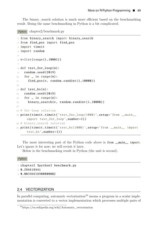
![50 • A Tour of Data Science: Learn R and Python in Parallel
operands simultaneously by compilers that feature auto-vectorization. For example,
let’s calculate the element-wise sum of two arrays x and y of the same length in C
programming language.
1 int x[4] = {1,2,3,4};
2 int y[4] = {0,1,2,3};
3 int z[4];
4 for (int i=0;i<4;i++){
5 z[i]=x[i]+y[i];
6 }
The C code above might be vectorized by the compiler so that the actual number
of iterations performed could be less than 4. If 4 pairs of operands are processed
at once, there would be only 1 iteration. Automatic vectorization may make the
program run much faster in some languages like C. However, when we talk about
vectorization in R/Python, it is different from automatic vectorization. Vectorization
in R/Python usually refers to the human effort paid to avoid for-loops. First, let’s
see some examples of how for-loops may slow your programs in R/Python.
R
chapter2/vectorization_1.R
1 library(microbenchmark)
2
3 # generate n standard normal r.v
4 rnorm_loop = function(n){
5 x=rep(0,n)
6 for (i in 1:n) {x[i]=rnorm(1)}
7 }
8
9 rnorm_vec = function(n){
10 x=rnorm(n)
11 }
12
13 n=100
14 # for loop
15 print(microbenchmark(rnorm_loop(n),times=1000))
16 # vectorize
17 print(microbenchmark(rnorm_vec(n),times=1000))
Running the R code produces the following result on my local machine.
R
1 > source(’vectorization_1.R’)](https://image.slidesharecdn.com/a-tour-of-data-science-learn-r-and-python-in-parallel-1st-edition-241027161058-87cda925/85/a-tour-of-data-science-learn-r-and-python-in-parallel-1st-edition-pdf-61-320.jpg)
![More on R/Python Programming • 51
2 Unit: microseconds
3 expr min lq mean median uq max
neval
4 rnorm_loop(n) 131.622 142.699 248.7603 145.3995 270.212 16355.6
1000
5 Unit: microseconds
6 expr min lq mean median uq max neval
7 rnorm_vec(n) 6.696 7.128 10.87463 7.515 8.291 2422.338 1000
Python
1 import timeit
2 import numpy as np
3
4 def rnorm_for_loop(n):
5 x=[0]∗n # create a list with n 0s
6 np.random.seed(2019)
7 for _ in range(n):
8 np.random.normal(0,1,1)
9
10 def rnorm_vec(n):
11 np.random.seed(2019)
12 x = np.random.normal(0,1,n)
13
14 print("for loop")
15 print(f’{timeit.timeit("rnorm_for_loop(100)",setup="from
__main__ import rnorm_for_loop",number=1000):.6f} seconds’)
16 print("vectorized")
17 print(f’{timeit.timeit("rnorm_vec(100)",setup="from __main__
import rnorm_vec",number=1000):.6f} seconds’)
Please note that in this Python example we are using the random submodule of
numpy module instead of the built-in random module since random module doesn’t
provide the vectorized version of random number generation function. Running the
Python code results in the following on my local machine.
Python
1 chapter2 $python3.7 vectorization_1.py
2 for loop
3 0.258466 seconds
4 vectorized
5 0.008213 seconds](https://image.slidesharecdn.com/a-tour-of-data-science-learn-r-and-python-in-parallel-1st-edition-241027161058-87cda925/85/a-tour-of-data-science-learn-r-and-python-in-parallel-1st-edition-pdf-62-320.jpg)
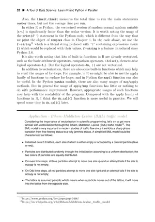
![More on R/Python Programming • 53
The BML model specified above is implemented in both R/Python as follows to
illustrate the usage of vectorization.
R chapter2/BML.R
1 library(R6)
2 BML = R6Class(
3 "BML",
4 public = list(
5 # alpha is the parameter of the uniform distribution to
control particle distribution ’s density
6 # m∗n is the dimension of the lattice
7 alpha = NULL,
8 m = NULL,
9 n = NULL,
10 lattice = NULL,
11 initialize = function(alpha, m, n) {
12 self$alpha = alpha
13 self$m = m
14 self$n = n
15 self$initialize_lattice()
16 },
17 initialize_lattice = function() {
18 # 0 −> empty site
19 # 1 −> blue particle
20 # 2 −> red particle
21 u = runif(self$m ∗ self$n)
22 # the usage of L is to make sure the elements in particles
are of type integer;
23 # otherwise they would be created as double
24 particles = rep(0L, self$m ∗ self$n)
25 # doing inverse transform sampling
26 particles[(u > self$alpha) &
27 (u <= (self$alpha + 1.0) / 2)] = 1L
28 particles[u > (self$alpha + 1.0) / 2] = 2L
29 self$lattice = array(particles , c(self$m, self$n))
30 },
31 odd_step = function() {
32 blue.index = which(self$lattice == 1L, arr.ind = TRUE)
33 # make a copy of the index
34 blue.up.index = blue.index
35 # blue particles move 1 site up
36 blue.up.index[, 1] = blue.index[, 1] − 1L
37 # periodic boundary condition
38 blue.up.index[blue.up.index[, 1] == 0L, 1] = self$m](https://image.slidesharecdn.com/a-tour-of-data-science-learn-r-and-python-in-parallel-1st-edition-241027161058-87cda925/85/a-tour-of-data-science-learn-r-and-python-in-parallel-1st-edition-pdf-64-320.jpg)
![54 • A Tour of Data Science: Learn R and Python in Parallel
39 # find which moves are feasible
40 blue.movable = self$lattice[blue.up.index] == 0L
41 # move blue particles one site up
42 # drop=FALSE prevents the 2D array degenerates to 1D array
43 self$lattice[blue.up.index[blue.movable , , drop = FALSE]]
= 1L
44 self$lattice[blue.index[blue.movable , , drop = FALSE]] = 0
L
45 },
46 even_step = function() {
47 red.index = which(self$lattice == 2L, arr.ind = TRUE)
48 # make a copy of the index
49 red.right.index = red.index
50 # red particles move 1 site right
51 red.right.index[, 2] = red.index[, 2] + 1L
52 # periodic boundary condition
53 red.right.index[red.right.index[, 2] == (self$n + 1L), 2]
= 1
54 # find which moves are feasible
55 red.movable = self$lattice[red.right.index] == 0L
56 # move red particles one site right
57 self$lattice[red.right.index[red.movable , , drop = FALSE]]
= 2L
58 self$lattice[red.index[red.movable , , drop = FALSE]] = 0L
59 }
60 )
61 )
Now we can create a simple BML system on a 5 × 5 lattice using the R code
above.
R
1 > source(’BML.R’)
2 > set.seed(2019)
3 > bml=BML$new(0.4,5,5)
4 > bml$lattice
5 [,1] [,2] [,3] [,4] [,5]
6 [1,] 2 0 2 1 1
7 [2,] 2 2 1 0 1
8 [3,] 0 0 0 2 2
9 [4,] 1 0 0 0 0
10 [5,] 0 1 1 1 0
11 > bml$odd_step()
12 > bml$lattice](https://image.slidesharecdn.com/a-tour-of-data-science-learn-r-and-python-in-parallel-1st-edition-241027161058-87cda925/85/a-tour-of-data-science-learn-r-and-python-in-parallel-1st-edition-pdf-65-320.jpg)
![More on R/Python Programming • 55
13 [,1] [,2] [,3] [,4] [,5]
14 [1,] 2 0 2 1 0
15 [2,] 2 2 1 0 1
16 [3,] 1 0 0 2 2
17 [4,] 0 1 1 1 0
18 [5,] 0 0 0 0 1
19 > bml$even_step()
20 > bml$lattice
21 [,1] [,2] [,3] [,4] [,5]
22 [1,] 0 2 2 1 0
23 [2,] 2 2 1 0 1
24 [3,] 1 0 0 2 2
25 [4,] 0 1 1 1 0
26 [5,] 0 0 0 0 1
In the initialization step, we used the inversion sampling approach13
to generate
the status of each site. Inversion sampling method is a basic but powerful approach
to generate r.v. from any probability distribution given its cumulative distribution
function (CDF). We will talk more about sampling technique in Chapter 4.
Python
1 import numpy as np
2
3 class BML:
4 def __init__(self, alpha, m, n):
5 self.alpha = alpha
6 self.shape = (m, n)
7 self.initialize_lattice()
8
9 def initialize_lattice(self):
10 u = np.random.uniform(0.0, 1.0, self.shape)
11 # instead of using default list, we use np.array to
create the lattice
12 self.lattice = np.zeros_like(u, dtype=int)
13 # the parentheses below can’t be ignored
14 self.lattice[(u > self.alpha) & (u <= (1.0+self.alpha)
/2.0)] = 1
15 self.lattice[u > (self.alpha+1.0)/2.0] = 2
16
17 def odd_step(self):
18 # please note that np.where returns a tuple which is
immutable
13
https://en.wikipedia.org/wiki/Inverse_transform_sampling](https://image.slidesharecdn.com/a-tour-of-data-science-learn-r-and-python-in-parallel-1st-edition-241027161058-87cda925/85/a-tour-of-data-science-learn-r-and-python-in-parallel-1st-edition-pdf-66-320.jpg)
![56 • A Tour of Data Science: Learn R and Python in Parallel
19 blue_index = np.where(self.lattice == 1)
20 blue_index_i = blue_index[0] − 1
21 blue_index_i[blue_index_i < 0] = self.shape[0]−1
22 blue_movable = self.lattice[(blue_index_i , blue_index
[1])] == 0
23 self.lattice[(blue_index_i[blue_movable],
24 blue_index[1][blue_movable])] = 1
25 self.lattice[(blue_index[0][blue_movable],
26 blue_index[1][blue_movable])] = 0
27
28 def even_step(self):
29 red_index = np.where(self.lattice == 2)
30 red_index_j = red_index[1] + 1
31 red_index_j[red_index_j == self.shape[1]] = 0
32 red_movable = self.lattice[(red_index[0], red_index_j)]
== 0
33 self.lattice[(red_index[0][red_movable],
34 red_index_j[red_movable])] = 2
35 self.lattice[(red_index[0][red_movable],
36 red_index[1][red_movable])] = 0
The Python implementation is also given.
R
1 >>> import numpy as np
2 >>> np.random.seed(2019)
3 >>> from BML import BML
4 >>> bml=BML(0.4,5,5)
5 >>> bml.lattice
6 array([[2, 0, 1, 1, 2],
7 [0, 2, 2, 2, 1],
8 [1, 0, 0, 2, 0],
9 [2, 0, 1, 0, 2],
10 [1, 1, 0, 2, 1]])
11 >>> bml.odd_step()
12 >>> bml.lattice
13 array([[2, 0, 0, 1, 2],
14 [1, 2, 2, 2, 1],
15 [0, 0, 1, 2, 0],
16 [2, 1, 0, 0, 2],
17 [1, 0, 1, 2, 1]])
18 >>> bml.even_step()
19 >>> bml.lattice
20 array([[0, 2, 0, 1, 2],](https://image.slidesharecdn.com/a-tour-of-data-science-learn-r-and-python-in-parallel-1st-edition-241027161058-87cda925/85/a-tour-of-data-science-learn-r-and-python-in-parallel-1st-edition-pdf-67-320.jpg)
![More on R/Python Programming • 57
21 [1, 2, 2, 2, 1],
22 [0, 0, 1, 0, 2],
23 [2, 1, 0, 0, 2],
24 [1, 0, 1, 2, 1]])
Please note that although we have imported numpy in BML.py, we import it again
in the code above in order to set the random seed. If we change the line to from
BML import ∗, we don’t need to import numpy again. But it is not recommended to
import ∗ from a module.
2.5 EMBARRASSINGLY PARALLELISM IN R/PYTHON
According to the explanation in wikipedia14
, single-threading is the processing of one
command at a time, and its opposite is multithreading. A process is the instance of a
computer program executed by one or many threads15
. Multithreading is not the same
as parallelism. In a single processor environment, the processor can switch execution
between threads, which results in concurrent execution. However, it is possible a
process with multithreads runs on a multiprocessor environment and each of the
threads on a separate processor, which results in parallel execution.
Both R and Python are single-threaded. In Python, there is a threading pack
age16
, which supports multithreading on a single core. It may suit some specific tasks.
For example, in web scraping multithreading on a single core may be able to speed
up the program if the download time is in excess of the CPU processing time.
Now let’s talk about embarrassingly parallelism by multiprocessing. An embar
rassingly parallel problem is one where little or no effort is needed to separate the
problem into a number of parallel tasks17
. In R there are various packages sup
porting multiprocessing on multiple CPU cores, for example, the parallel package,
which is my favorite one. In Python, there are also some available modules, such as
multiprocessing, joblib and concurrent.futures.
Let’s see an application of embarrassingly parallelism to calculate π using Monte
Carlo simulation18
.
Application - Monte Carlo simulation to estimate π via parallelization
Monte Carlo simulation provides a simple and straightforward way to estimate π. We know
the area of a circle with radius 1 is just π. Thus, we can convert the original problem of π
calculation to a new problem, i.e., how to calculate the area of a circle with radius 1. We
also know the area of a square with side length 2 is equal to 4. Thus, π can be calculated
as 4rc/s where rc/s denotes the ratio of areas of a circle with radius 1 and a square with
side length 2. Now the problem is how to calculate the ratio rc/s? When we randomly throw
14
https://en.wikipedia.org/wiki/Thread_(computing)
15
https://en.wikipedia.org/wiki/Process_(computing)
16
https://docs.python.org/3.7/library/threading.html
17
https://en.wikipedia.org/wiki/Embarrassingly_parallel
18
https://en.wikipedia.org/wiki/Monte_Carlo_method](https://image.slidesharecdn.com/a-tour-of-data-science-learn-r-and-python-in-parallel-1st-edition-241027161058-87cda925/85/a-tour-of-data-science-learn-r-and-python-in-parallel-1st-edition-pdf-68-320.jpg)
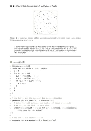
![More on R/Python Programming • 59
23 p = array(runif(n∗2,−1,1), c(n,2))
24 sum((p[,1]^2+p[,2]^2) <=1)
25 }
26
27 pi_naive = function(n) cat(’naive: pi −’, 4∗count_inside_point(n
)/n, ’n’)
28
29 pi_parallel = function(n) cat(’parallel: pi −’, 4∗sum(
generate_points_parallel(n))/n, ’n’)
30
31 pi_vectorized = function(n) cat(’vectorized: pi −’, 4∗sum(
generate_points_vectorized(n))/n, ’n’)
In the above R code snippet, we use the function mclapply which is not currently
available on some operation systems19
. When it is not available, we may consider
using parLapply instead.
Python chapter2/pi.py
1 # now let’s try the parallel approach
2 # each process uses the same seed, which is not desired
3 def generate_points_parallel(n):
4 pool = mp.Pool()
5 # we ask each process to generate n//mp.cpu_count() points
6 return pool.map(count_inside_point , [n//mp.cpu_count()]∗mp.
cpu_count())
7
8 # set seed for each process
9 # first, let’s define a helper function
10 def helper(args):
11 n, s = args
12 seed(s)
13 return count_inside_point(n)
14
15 def generate_points_parallel_set_seed(n):
16 pool = mp.Pool() # we can also specify the number of
processes by Pool(number)
17 # we ask each process to generate n//mp.cpu_count() points
18 return pool.map(helper , list(zip([n//mp.cpu_count()]∗mp.
cpu_count(),range(mp.cpu_count()))))
19
20 # another optimization via vectorization
21 def generate_points_vectorized(n):
19
https://stat.ethz.ch/R-manual/R-devel/library/parallel/doc/parallel.pdf](https://image.slidesharecdn.com/a-tour-of-data-science-learn-r-and-python-in-parallel-1st-edition-241027161058-87cda925/85/a-tour-of-data-science-learn-r-and-python-in-parallel-1st-edition-pdf-70-320.jpg)
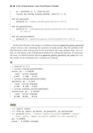
![More on R/Python Programming • 61
6 >>> print(f’parallel − {timeit.timeit("pi_parallel(1000000)",
setup="from __main__ import pi_parallel",number=1):.6f}
seconds’)
7 pi: 3.141032
8 parallel − 2.204697 seconds
9 >>> print(f’vectorized − {timeit.timeit("pi_vectorized(1000000)
",setup="from __main__ import pi_vectorized",number=1):.6f}
seconds’)
10 pi: 3.139936
11 vectorized − 0.148950 seconds
We see the winner in this example is vectorization, and the parallel solution is
better than the naive solution. However, when the problem cannot be vectorized we
may use parallelization to achieve better performance.
2.6 EVALUATION STRATEGY
R is a lazy programming language since it uses lazy evaluation by default [13]. Lazy
evaluation strategy delays the evaluation of an expression until its value is needed.
When an expression in R is evaluated, it follows an outermost reduction order in gen
eral. But Python is not a lazy programming language and the expression in Python
follows an innermost reduction order. The code snippets below illustrate the inner
most reduction vs. outermost reduction.
R Python
1 > divide = function(x, y){ 1 >>> def divide(x, y):
stopifnot(y!=0);return(x return x/y
/y)} 2 >>> def power(x, p):
1
2 > power = return if p==0
function(x, p){ else x p
if (p==0) 1 else x^p}
3 >>> power(
∗∗
divide(1,0),0)
3 > power(divide(1,0),2)
4 Traceback (most recent call
4 Error in divide(1, 0) : y !
= 0 last):
is not TRUE
5 > power(divide(1,0),0) 5 File "<stdin>", line 1,
6 [1] 1 in <module >
6 File "<stdin>", line 1,
in divide
7 ZeroDivisionError: division
by zero
Because of the outermost reduction order, the R code snippet evaluates the func
tion power first and since if the second argument is 0 the first argument is not required
to evaluate. Thus, the function call returns 1. But the Python code snippet first eval
uates the function call of divide and an exception is raised because of division by
zero.
Although Python is an eager language, it is possible to simulate the lazy eval](https://image.slidesharecdn.com/a-tour-of-data-science-learn-r-and-python-in-parallel-1st-edition-241027161058-87cda925/85/a-tour-of-data-science-learn-r-and-python-in-parallel-1st-edition-pdf-72-320.jpg)
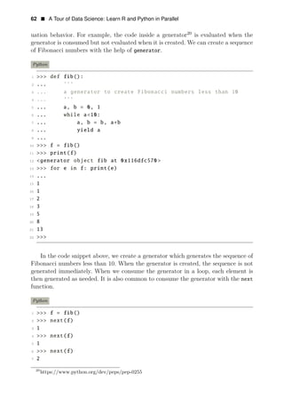
![The purpose of this section is not to teach C/C++. If you know how to write C/C++
then it may help to improve the performance of R/Python program.
It is recommended to use vectorization technique to speed up your program when
ever possible. But what if it’s infeasible to vectorize the algorithm? One potential
option is to use C/C++ in the R/Python code. According to my limited experience,
it is much easier to use C/C++ in R with the help of Rcpp package than in Python.
In Python, more options are available but not as straightforward as the solution of
Rcpp. In this section, let’s use 21
Cython .
Actually, Cython itself is a programming language written in Python and C. In
Rcpp we can write C++ code directly and use it in native R code. With the help of
Cython, we can write python-like code which is able to be compiled to C or C++
and automatically wrapped into python-importable modules. Cython could also wrap
independent C or C++ code into python-importable modules.
Let’s see how to calculate Fibonacci numbers with these tools. The first step is
to install Rcpp package in R and the Cython module (use pip) in Python. Once they
are installed, we can write the code in C++ directly for R. As for Cython, we write
the python-like code which will be compiled to C/C++ later.
R chapter2/Fibonacci.cpp Python chapter2/Fibonacci.pyx
1 #include <Rcpp.h> 1 #!python
2 using namespace Rcpp; 2 #cython: language_level=3
3 3
4 // [[Rcpp::export]] 4 cdef int Fibonacci_c(int n):
5 int Fibonacci(int n) { 5 if n==1 or n==2:
6 if (n==1 or n==2){ 6 return 1
7 return 1; 7 return Fibonacci_c(n−1)
8 } + Fibonacci_c(n
9
−2)
return Fibonacci(n−1)+ 8
Fibonacci(n−2); 9 def Fibonacci_static(n):
10 } 10 return Fibonacci_c(n)
11
12 def Fibonacci(n):
13 if n==1 or n==2:
14 return 1
21
https://en.wikipedia.org/wiki/Cython
More on R/Python Programming • 63
8 >>> next(f)
9 3
10 >>> next(f)
11 5
2.7 SPEED UP WITH C/C++ IN R/PYTHON](https://image.slidesharecdn.com/a-tour-of-data-science-learn-r-and-python-in-parallel-1st-edition-241027161058-87cda925/85/a-tour-of-data-science-learn-r-and-python-in-parallel-1st-edition-pdf-74-320.jpg)
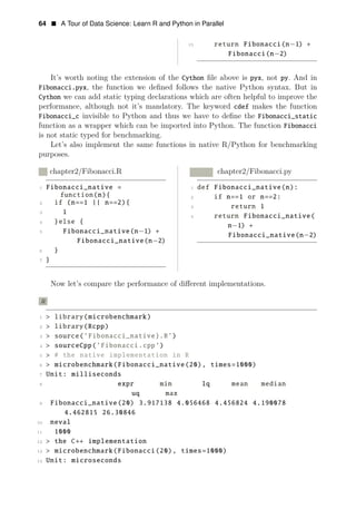
![More on R/Python Programming • 65
15 expr min lq mean median uq max
neval
16 Fibonacci(20) 14.251 14.482 15.81708 14.582 14.731 775.095
1000
The native implementation in R is much slower than the C++ implementation
(see the difference of units).
Python
1 >>> import pyximport
2 >>> pyximport.install()
3 (None, <pyximport.pyximport.PyxImporter object at 0x1056f9f98 >)
4 >>> from Fibonacci import Fibonacci_static , Fibonacci
5 >>> from Fibonacci_native import Fibonacci_native
6 >>> import timeit
7 >>> print(f’{timeit.timeit("Fibonacci_native(20)",setup="from
__main__ import Fibonacci_native",number=1000):.6f} seconds’
)
8 1.927359 seconds
9 >>> print(f’{timeit.timeit("Fibonacci(20)",setup="from __main__
import Fibonacci",number=1000):.6f} seconds’)
10 0.316726 seconds
11 >>> print(f’{timeit.timeit("Fibonacci_static(20)",setup="from
__main__ import Fibonacci_static",number=1000):.6f} seconds’
)
12 0.012741 seconds
The results show the static typed implementation is the fastest, and the native
implementation in pure Python is the slowest. Again the time measured by timeit.
timeit is the total time to run the main statement 1000 times. The average time per
run of Fibonacci_static function is close to the average time per run of Fibonacci
in R.
2.8 A FIRST IMPRESSION OF FUNCTIONAL PROGRAMMING
Functional (programming) languages define programs as mathematical functions and
treat them as first-class22
. In pure functional programming, a function takes input and
returns output without making any side effect. A side effect means a state variable
outside the function is modified. For example, printing the value of a variable inside
a function is a side effect.
Both R and Python are not purely functional languages per se, although R be
haves more functionally than Python [5]. If you wonder why the return function
22
https://en.wikipedia.org/wiki/List_of_programming_languages_by_type#Functional_languages](https://image.slidesharecdn.com/a-tour-of-data-science-learn-r-and-python-in-parallel-1st-edition-241027161058-87cda925/85/a-tour-of-data-science-learn-r-and-python-in-parallel-1st-edition-pdf-76-320.jpg)
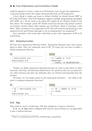
![More on R/Python Programming • 67
R Python
1 > Map(function(x) x x, 1 >>> map(
c(1:3))
∗
lambda e: e∗∗2, [1,2,3])
2 [[1]] 2 <map object at 0x1033e3160 >
3 [1] 1 3 >>> list(map(
2
4 lambda x: x , [1,2,3]))
4 [1, 4, 9]
∗∗
5 [[2]]
5 >>> list(map(lambda x, y: x
6 [1] 4
∗
y, [1,2,3], [4,5,6]))
7
6 [4, 10, 18]
8 [[3]]
9 [1] 9
10 > Map(function(x, y) x y,
c(1:3), c(4:6))
∗
11 [[1]]
12 [1] 4
13
14 [[2]]
15 [1] 10
16
17 [[3]]
18 [1] 18
There are a few things to note from the code snippets above. First, the returned
value from Map in R is a list rather than a vector. That is because Map is just a wrapper
of mapply function in R, and the SIMPLIFY argument is set to FALSE. If we want to
get a vector value returned, just use mapply instead.
R
1 > mapply(function(x, y) x∗y, c(1:3), c(4:6), SIMPLIFY=TRUE)
2 [1] 4 10 18
The returned value from map in Python is a map object which is an iterator. The
generator function we have seen before is also an iterator. To use an iterator, we
could convert it to a list, or get the next value using the next function, or just use a
for loop.
Python
1 >>> # use next on an iterator
2 >>> o=map(lambda x, y: x∗y, [1,2,3], [4,5,6])
3 >>> next(o)
4 4
5 >>> next(o)
6 10](https://image.slidesharecdn.com/a-tour-of-data-science-learn-r-and-python-in-parallel-1st-edition-241027161058-87cda925/85/a-tour-of-data-science-learn-r-and-python-in-parallel-1st-edition-pdf-78-320.jpg)
![68 • A Tour of Data Science: Learn R and Python in Parallel
7 >>> o=map(lambda x, y: x∗y, [1,2,3], [4,5,6])
8 >>> # use for loop on an iterator
9 >>> for e in o:print(e)
10 ...
11 4
12 10
13 18
14 >>> # convert an iterator to a list
15 >>> o=map(lambda x, y: x∗y, [1,2,3], [4,5,6])
16 >>> list(o)
17 [4, 10, 18]
2.8.3 Filter
Similar to map, the first argument to Filter in R and filter in Python is also a
function. This function is used to get the elements which satisfy a certain condition
specified in the first argument. For example, we can use it to get the even numbers.
R Python
1 > Filter(function(x) x 1 >>> list(filter(
%%2==0, c(0:10)) lambda e: e%2==0,
range(11)))
2 [1] 0 2 4 6 8 10
2 [0, 2, 4, 6, 8, 10]
2.8.4 Reduce
Reduce behaves a bit differently from Map and Filter. The first argument is a function
with exactly two arguments. The second argument is a sequence, on each element of
which the first function argument will be applied from left to right. And there is one
optional argument called initializer. When the initializer is provided, it will be used
as the first argument of the function argument of Reduce. The examples below depict
how it works.
R
1 > Reduce(function(x, y) x+2
∗y, c(1,2,3))
2 [1] 11
3 > Reduce(function(x, y) x+2
∗y, c(1,2,3), 1)
4 [1] 13
Python
1 >>> from functools import
reduce
2 >>> reduce(lambda x, y:x+2∗y
, [1,2,3])
3 11
4 >>> reduce(
lambda x, y:x+2∗y,
range(1,4), 1)
5 13
Please note that in order to use reduce in Python, we have to import it from the
functools module.](https://image.slidesharecdn.com/a-tour-of-data-science-learn-r-and-python-in-parallel-1st-edition-241027161058-87cda925/85/a-tour-of-data-science-learn-r-and-python-in-parallel-1st-edition-pdf-79-320.jpg)
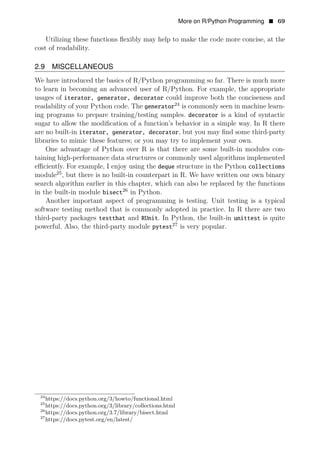

![Upon receiving feedback and requests from readers on the first few chap
ters, I decided to devote a whole chapter to the introduction of data
.table and pandas. Of course, there are many other great data analysis tools in both
R and Python. For example, many R users like using dplyr to build up data analysis
pipelines. The performance of data.table is superior and that is the main reason I
feel there is no need to use other tools for the same tasks in R. But if you are a big fan
of the pipe operator %>% you may use data.table and dplyr together. Regarding the
big data ecosystem, Apache Spark has API in both R and Python. Recently, there
are also some emerging projects aiming at better usability and performance, such as
1
Apache Arrow , 2
Modin .
3.1 SQL
Similar to the previous chapters, I will introduce the tools side by side. However,
I feel before diving into the world of data.table and pandas, it is better to talk a
little bit about 3
SQL . SQL is a Query language designed for managing data in relational
database management system (RDBMS). Some of the most popular RDBMSs include
MS SQL Server, MySQL, PostgreSQL, etc. Different RDBMSs may use SQL languages
with major or subtle differences.
If you have never used RDBMS you may wonder why we need it.
• first, we need a system to store the data;
• second, we also need a system that allows us to easily access, manage and
update the data.
In this chapter, we will use the public mtcars dataset as an example. This dataset
was available in R4
and originally it was reported in [11].
Let’s assume there is a table mtcars in a database (I’m using sqlite3 in this book)
and see some simple tasks we can do with SQL queries.
1
https://arrow.apache.org
2
https://github.com/modin-project/modin
3
https://en.wikipedia.org/wiki/SQL
4
https://stat.ethz.ch/R-manual/R-devel/library/datasets/html/mtcars.html
C H A P T E R 3
data.table and pandas
71](https://image.slidesharecdn.com/a-tour-of-data-science-learn-r-and-python-in-parallel-1st-edition-241027161058-87cda925/85/a-tour-of-data-science-learn-r-and-python-in-parallel-1st-edition-pdf-82-320.jpg)
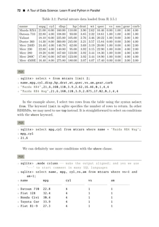
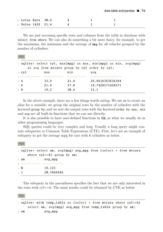
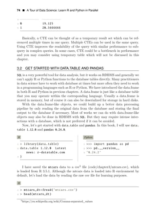
![data.table and pandas • 75
3 name mpg cyl disp hp drat wt qsec vs am
gear carb
4 1: Mazda RX4 21.0 6 160 110 3.90 2.620 16.46 0 1
4 4
5 2: Mazda RX4 Wag 21.0 6 160 110 3.90 2.875 17.02 0 1
4 4
6 3: Datsun 710 22.8 4 108 93 3.85 2.320 18.61 1 1
4 1
7 4: Hornet 4 Drive 21.4 6 258 110 3.08 3.215 19.44 1 0
3 1
8 5: Hornet Sportabout 18.7 8 360 175 3.15 3.440 17.02 0 0
3 2
9 6: Valiant 18.1 6 225 105 2.76 3.460 20.22 1 0
3 1
Python
1 >>> import pandas as pd
2 >>> mtcars_df=pd.read_csv(’mtcars.csv’)
3 >>> mtcars_df.head(5)
4 name mpg cyl disp hp ... qsec vs am
gear carb
5 0 Mazda RX4 21.0 6 160.0 110 ... 16.46 0 1
4 4
6 1 Mazda RX4 Wag 21.0 6 160.0 110 ... 17.02 0 1
4 4
7 2 Datsun 710 22.8 4 108.0 93 ... 18.61 1 1
4 1
8 3 Hornet 4 Drive 21.4 6 258.0 110 ... 19.44 1 0
3 1
9 4 Hornet Sportabout 18.7 8 360.0 175 ... 17.02 0 0
3 2
10
11 [5 rows x 12 columns]
The type of mtcars_dt is data.table, not data.frame. Here we use the fread
function from data.table to read a file and the output type is a data.table directly.
Regarding reading csv in R, a very good package is readr for very large files, but the
output has a data.frame type. In practice, it is very common to convert a data.frame
to data.table with the function as.data.table.](https://image.slidesharecdn.com/a-tour-of-data-science-learn-r-and-python-in-parallel-1st-edition-241027161058-87cda925/85/a-tour-of-data-science-learn-r-and-python-in-parallel-1st-edition-pdf-86-320.jpg)
![76 • A Tour of Data Science: Learn R and Python in Parallel
3.3 INDEXING & SELECTING DATA
Before introducing the indexing rules in data.table and pandas, it’s better to under
stand the key in data.table and the index in pandas.
What is the key in a data.table? We have talked about RDBMS and SQL in the
previous section. With select from where we can easily access specific rows satisfying
certain conditions. When the database table is too large, a database index is used to
improve the performance of data retrieval operations. Essentially, a database index
is a data structure, and to maintain the data structure, additional cost (for example,
space) may be required. The reason to use key in data.table and index in pandas is
very similar. Now let’s see how to set key and index.
R
1 > setkey(mtcars_dt ,name)
2 > key(mtcars_dt)
3 [1] "name"
4 > head(mtcars_dt ,5)
5 name mpg cyl disp hp drat wt qsec vs am
gear carb
6 1: AMC Javelin 15.2 8 304 150 3.15 3.435 17.30 0 0
3 2
7 2: Cadillac Fleetwood 10.4 8 472 205 2.93 5.250 17.98 0 0
3 4
8 3: Camaro Z28 13.3 8 350 245 3.73 3.840 15.41 0 0
3 4
9 4: Chrysler Imperial 14.7 8 440 230 3.23 5.345 17.42 0 0
3 4
10 5: Datsun 710 22.8 4 108 93 3.85 2.320 18.61 1 1
4 1
Python
1 >>> mtcars_df.set_index(’name’,inplace=True)
2 >>> mtcars_df.index.name
3 ’name’
4 >>> mtcars_df.head(5)
5 mpg cyl disp hp drat ... qsec vs
am gear carb
6 name ...
7 Mazda RX4 21.0 6 160.0 110 3.90 ... 16.46 0
1 4 4
8 Mazda RX4 Wag 21.0 6 160.0 110 3.90 ... 17.02 0
1 4 4
9 Datsun 710 22.8 4 108.0 93 3.85 ... 18.61 1
1 4 1](https://image.slidesharecdn.com/a-tour-of-data-science-learn-r-and-python-in-parallel-1st-edition-241027161058-87cda925/85/a-tour-of-data-science-learn-r-and-python-in-parallel-1st-edition-pdf-87-320.jpg)
![data.table and pandas • 77
10 Hornet 4 Drive 21.4 6 258.0 110 3.08 ... 19.44 1
0 3 1
11 Hornet Sportabout 18.7 8 360.0 175 3.15 ... 17.02 0
0 3 2
There are quite a few things worth noting from the above code snippets. When
we use the setkey function the quotes for the column name is optional. So setkey(
mtcars_dt, name) is equivalent to setkey(mtcars_dt, ’name’). But in pandas, quotes
are required. The effect of setkey is in place, which means no copies of the data are
made at all. But in pandas, by default set_index set the index on a copy of the data
and the modified copy is returned. Thus, in order to make the effect in place, we have
set the argument inplace=True explicitly. Another difference is that setkey would
sort the original data in place automatically but set_index does not. It’s also worth
noting every pandas data.frame has an index; and by default it is numpy.arange(n)
where n is the number of rows. But there is no default key in a data.table.
In the above example, we only use a single column as the key/index. It is possible
to use multiple columns as well.
R Python
1 > setkeyv(mtcars_dt ,c(’cyl’, 1 >>> mtcars_df.set_index([’
’gear’)) cyl’,’gear’],inplace=
True)
2 > key(mtcars_dt)
2
3 [1]
>>> mtcars_df.index.names
"cyl" "gear"
3 FrozenList([’cyl’, ’gear’])
To use multiple columns as the key in data.table, we use the function setkeyv. It
is also interesting that we have to use index.names rather than index.name to get the
multiple column names of the index (which is called MultiIndex) in pandas. There
are duplicated combinations of (cyl, gear) in the data, which implies key or index
could be duplicated.
Once the key/index set, we can access rows with given indices fast.
R
1 > mtcars_dt[’Merc 230’]
2 name mpg cyl disp hp drat wt qsec vs am gear carb
3 1: Merc 230 22.8 4 140.8 95 3.92 3.15 22.9 1 0 4 2
4 > mtcars_dt[c(’Merc 230’,’Camaro Z28’)] # multiple values of a
single index
5 name mpg cyl disp hp drat wt qsec vs am gear carb
6 1: Merc 230 22.8 4 140.8 95 3.92 3.15 22.90 1 0 4 2
7 2: Camaro Z28 13.3 8 350.0 245 3.73 3.84 15.41 0 0 3 4
8 > setkeyv(mtcars_dt ,c(’cyl’,’gear’))
9 > mtcars_dt[.(6,4)] # work with key vector using .()](https://image.slidesharecdn.com/a-tour-of-data-science-learn-r-and-python-in-parallel-1st-edition-241027161058-87cda925/85/a-tour-of-data-science-learn-r-and-python-in-parallel-1st-edition-pdf-88-320.jpg)
![78 • A Tour of Data Science: Learn R and Python in Parallel
10 name mpg cyl disp hp drat wt qsec vs am gear
carb
11 1: Mazda RX4 21.0 6 160.0 110 3.90 2.620 16.46 0 1 4
4
12 2: Mazda RX4 Wag 21.0 6 160.0 110 3.90 2.875 17.02 0 1 4
4
13 3: Merc 280 19.2 6 167.6 123 3.92 3.440 18.30 1 0 4
4
14 4: Merc 280C 17.8 6 167.6 123 3.92 3.440 18.90 1 0 4
4
15 > mtcars_dt[.(c(6,8),c(4,3))] # key vector with multiple values
16 name mpg cyl disp hp drat wt qsec vs
am gear carb
17 1: Mazda RX4 21.0 6 160.0 110 3.90 2.620 16.46 0
1 4 4
18 2: Mazda RX4 Wag 21.0 6 160.0 110 3.90 2.875 17.02 0
1 4 4
19 3: Merc 280 19.2 6 167.6 123 3.92 3.440 18.30 1
0 4 4
20 4: Merc 280C 17.8 6 167.6 123 3.92 3.440 18.90 1
0 4 4
21 5: AMC Javelin 15.2 8 304.0 150 3.15 3.435 17.30 0
0 3 2
22 6: Cadillac Fleetwood 10.4 8 472.0 205 2.93 5.250 17.98 0
0 3 4
23 7: Camaro Z28 13.3 8 350.0 245 3.73 3.840 15.41 0
0 3 4
24 8: Chrysler Imperial 14.7 8 440.0 230 3.23 5.345 17.42 0
0 3 4
25 9: Dodge Challenger 15.5 8 318.0 150 2.76 3.520 16.87 0
0 3 2
26 10: Duster 360 14.3 8 360.0 245 3.21 3.570 15.84 0
0 3 4
27 11: Hornet Sportabout 18.7 8 360.0 175 3.15 3.440 17.02 0
0 3 2
28 12: Lincoln Continental 10.4 8 460.0 215 3.00 5.424 17.82 0
0 3 4
29 13: Merc 450SE 16.4 8 275.8 180 3.07 4.070 17.40 0
0 3 3
30 14: Merc 450SL 17.3 8 275.8 180 3.07 3.730 17.60 0
0 3 3
31 15: Merc 450SLC 15.2 8 275.8 180 3.07 3.780 18.00 0
0 3 3
32 16: Pontiac Firebird 19.2 8 400.0 175 3.08 3.845 17.05 0
0 3 2](https://image.slidesharecdn.com/a-tour-of-data-science-learn-r-and-python-in-parallel-1st-edition-241027161058-87cda925/85/a-tour-of-data-science-learn-r-and-python-in-parallel-1st-edition-pdf-89-320.jpg)
![data.table and pandas • 79
Here is a bit of explanation for the code above. We can simply use [] to access the
rows with the specified key values if the key has a character type. But if the key has a
numeric type, list() is required to enclose the key values. In data.table, .() is just
an alias of list(), which means we would get the same results with mtcars_dt[list
(6,4)]. Of course, we can use also do mtcars_dt[.(’Merc 230’)] which is equivalent
to mtcars_dt[.(’Merc 230’)].
Python
1 >>> mtcars_df.loc[’Merc 230’]
2 mpg 22.80
3 cyl 4.00
4 disp 140.80
5 hp 95.00
6 drat 3.92
7 wt 3.15
8 qsec 22.90
9 vs 1.00
10 am 0.00
11 gear 4.00
12 carb 2.00
13 Name: Merc 230, dtype: float64
14 >>> mtcars_df.loc[[’Merc 230’,’Camaro Z28’]] # multiple values
of a single index
15 mpg cyl disp hp drat wt qsec vs am
gear carb
16 name
17 Merc 230 22.8 4 140.8 95 3.92 3.15 22.90 1 0
4 2
18 Camaro Z28 13.3 8 350.0 245 3.73 3.84 15.41 0 0
3 4
19
20 mtcars_df.set_index([’cyl’,’gear’],inplace=True)
21 >>> mtcars_df.loc[(6,4)] # work with MultiIndex using ()
22 mpg disp hp drat wt qsec vs am carb
23 cyl gear
24 6 4 21.0 160.0 110 3.90 2.620 16.46 0 1 4
25 4 21.0 160.0 110 3.90 2.875 17.02 0 1 4
26 4 19.2 167.6 123 3.92 3.440 18.30 1 0 4
27 4 17.8 167.6 123 3.92 3.440 18.90 1 0 4
28 >>> # you may notice that the name column disappeared; that
would be explained later](https://image.slidesharecdn.com/a-tour-of-data-science-learn-r-and-python-in-parallel-1st-edition-241027161058-87cda925/85/a-tour-of-data-science-learn-r-and-python-in-parallel-1st-edition-pdf-90-320.jpg)
![80 • A Tour of Data Science: Learn R and Python in Parallel
29 >>> mtcars_df.loc[[(6,4) ,(8,3)]] # MultiIndex with multiple
values
30 mpg disp hp drat wt qsec vs am carb
31 cyl gear
32 6 4 21.0 160.0 110 3.90 2.620 16.46 0 1 4
33 4 21.0 160.0 110 3.90 2.875 17.02 0 1 4
34 4 19.2 167.6 123 3.92 3.440 18.30 1 0 4
35 4 17.8 167.6 123 3.92 3.440 18.90 1 0 4
36 8 3 18.7 360.0 175 3.15 3.440 17.02 0 0 2
37 3 14.3 360.0 245 3.21 3.570 15.84 0 0 4
38 3 16.4 275.8 180 3.07 4.070 17.40 0 0 3
39 3 17.3 275.8 180 3.07 3.730 17.60 0 0 3
40 3 15.2 275.8 180 3.07 3.780 18.00 0 0 3
41 3 10.4 472.0 205 2.93 5.250 17.98 0 0 4
42 3 10.4 460.0 215 3.00 5.424 17.82 0 0 4
43 3 14.7 440.0 230 3.23 5.345 17.42 0 0 4
44 3 15.5 318.0 150 2.76 3.520 16.87 0 0 2
45 3 15.2 304.0 150 3.15 3.435 17.30 0 0 2
46 3 13.3 350.0 245 3.73 3.840 15.41 0 0 4
47 3 19.2 400.0 175 3.08 3.845 17.05 0 0 2
Compared to data.table, we need to use the loc method when accessing rows
based on index. The loc method also takes boolean conditions.
Python
1 >>> mtcars_df.loc[mtcars_df.mpg >30] # select the vehicles with
mpg>30
2 mpg disp hp drat wt qsec vs am carb
3 cyl gear
4 4 4 32.4 78.7 66 4.08 2.200 19.47 1 1 1
5 4 30.4 75.7 52 4.93 1.615 18.52 1 1 2
6 4 33.9 71.1 65 4.22 1.835 19.90 1 1 1
7 5 30.4 95.1 113 3.77 1.513 16.90 1 1 2
When using boolean conditions, loc could be ignored for convenience.
Python
1 >>> mtcars_df[mtcars_df.mpg>30] # ignore loc with boolean
conditions
2 mpg disp hp drat wt qsec vs am carb
3 cyl gear
4 4 4 32.4 78.7 66 4.08 2.200 19.47 1 1 1
5 4 30.4 75.7 52 4.93 1.615 18.52 1 1 2](https://image.slidesharecdn.com/a-tour-of-data-science-learn-r-and-python-in-parallel-1st-edition-241027161058-87cda925/85/a-tour-of-data-science-learn-r-and-python-in-parallel-1st-edition-pdf-91-320.jpg)
![data.table and pandas • 81
6 4 33.9 71.1 65 4.22 1.835 19.90 1 1 1
7 5 30.4 95.1 113 3.77 1.513 16.90 1 1 2
If the key/index is not needed, we can remove the key or reset the index. For
data.table we can set a new key to override the existing one which then becomes
a column. But in pandas, set_index method removes the existing index which also
disappears from the data.frame.
R
1 > key(mtcars_dt)
2 [1] "cyl" "gear"
3 > setkey(mtcars_dt , NULL) # remove the existing key
4 > key(mtcars_dt)
5 NULL
6 > setkey(mtcars_dt , ’gear’)
7 > key(mtcars_dt)
8 [1] "gear"
9 > setkey(mtcars_dt , ’name’) # override the existing key
10 > key(mtcars_dt)
11 [1] "name"
Python
1 >>> mtcars_df.index.names
2 FrozenList([’cyl’, ’gear’])
3 >>> mtcars_df.reset_index(inplace=True) # remove the existing
index
4 >>> mtcars_df.index.names
5 FrozenList([None])
6 >>> mtcars_df.set_index([’gear’], inplace=True)
7 >>> mtcars_df.index.name
8 ’gear’
9 >>> mtcars_df.columns # list all columns
10 Index([’cyl’, ’name’, ’mpg’, ’disp’, ’hp’, ’drat’, ’wt’, ’qsec’,
’vs’, ’am’,
11 ’carb’],
12 dtype=’object’)
13 >>> mtcars_df.set_index(’name’, inplace=True)
14 >>> mtcars_df.columns # the name column disappears
15 Index([’cyl’, ’mpg’, ’disp’, ’hp’, ’drat’, ’wt’, ’qsec’, ’vs’, ’
am’, ’carb’], dtype=’object’)
16 >>>](https://image.slidesharecdn.com/a-tour-of-data-science-learn-r-and-python-in-parallel-1st-edition-241027161058-87cda925/85/a-tour-of-data-science-learn-r-and-python-in-parallel-1st-edition-pdf-92-320.jpg)
![82 • A Tour of Data Science: Learn R and Python in Parallel
In Chapter 1, we introduced integer-based indexing for list/vector. It is also ap
plicable to data frame and data.table.
R
1 > mtcars_dt=fread(’mtcars.csv’)
2 > mtcars_dt[c(1,2,6),]
3 name mpg cyl disp hp drat wt qsec vs am gear
carb
4 1: Mazda RX4 21.0 6 160 110 3.90 2.620 16.46 0 1 4
4
5 2: Mazda RX4 Wag 21.0 6 160 110 3.90 2.875 17.02 0 1 4
4
6 3: Valiant 18.1 6 225 105 2.76 3.460 20.22 1 0 3
1
Python
1 >>> mtcars_df=pd.read_csv(’mtcars.csv’)
2 >>> mtcars_df.iloc[[0,1,5]] # again, indices in python are zero−
based.
3 name mpg cyl disp hp ... qsec vs am
gear carb
4 0 Mazda RX4 21.0 6 160.0 110 ... 16.46 0 1
4 4
5 1 Mazda RX4 Wag 21.0 6 160.0 110 ... 17.02 0 1
4 4
6 5 Valiant 18.1 6 225.0 105 ... 20.22 1 0
3 1
So far we have seen how to access specific rows. What about columns? Accessing
columns in data.table and pandas is quite straightforward. For data.table, we can
use $ sign to access a single column or a vector to specify multiple columns inside [].
For data.frame in pandas, we can use . to access a single column or a list to specify
multiple columns inside [].
R Python
1 > head(mtcars_dt$mpg,5) # 1 >>> mtcars_df.iloc[0:5].mpg.
access a single column values
2 [1] 21.0 21.0 22.8 21.4
2 array([21. , 21. , 22.8,
18.7}
21.4, 18.7])
3 > mtcars_dt[1:5,c(’mpg’,’
3 Name: mpg, dtype: float64
gear’)]
4 mpg gear 4 >>> mtcars_df[[’mpg’,’gear
’]].head(5)](https://image.slidesharecdn.com/a-tour-of-data-science-learn-r-and-python-in-parallel-1st-edition-241027161058-87cda925/85/a-tour-of-data-science-learn-r-and-python-in-parallel-1st-edition-pdf-93-320.jpg)
![data.table and pandas • 83
5 1: 21.0 4 5 mpg gear
6 2: 21.0 4 6 0 21.0 4
7 3: 22.8 4 7 1 21.0 4
8 4: 21.4 3 8 2 22.8 4
9 5: 18.7 3 9 3 21.4 3
10 4 18.7 3
In addition to passing a vector to access multiple columns in data.table, we can
also use the .(variable_1,variable_2,...).
R
1 > mtcars_dt[1:5,.(mpg,cyl,hp)] # without quotes for variables
2 mpg cyl hp
3 1: 21.5 4 97
4 2: 22.8 4 93
5 3: 24.4 4 62
6 4: 22.8 4 95
7 5: 32.4 4 66
It is also possible to do integer-based columns slicing.
R Python
1 > mtcars_dt[1:5,c(2,5,6)] # 1 >>> mtcars_df.iloc
the 2nd, the 5th and the [0:5,[1,4,5]] # the 2nd,
6th column
the 5th and the 6th
2 mpg hp drat column
3 1: 21.0 110 3.90 2 mpg hp drat
4 21.0 110 3.90 3
2: 0 21.0 110 3.90
5 3: 22.8 93 3.85 4 1 21.0 110 3.90
6 4: 21.4 110 3.08 5 2 22.8 93 3.85
7 5: 18.7 175 3.15 6 3 21.4 110 3.08
7 4 18.7 175 3.15
To access specific rows and specific columns, there are two strategies:
1. select rows and then select columns in a chain;
2. select rows and columns simultaneously.
Let’s see some examples.
R
1 > mtcars_dt=fread(’mtcars.csv’)
2 > setkey(mtcars_dt ,’gear’)](https://image.slidesharecdn.com/a-tour-of-data-science-learn-r-and-python-in-parallel-1st-edition-241027161058-87cda925/85/a-tour-of-data-science-learn-r-and-python-in-parallel-1st-edition-pdf-94-320.jpg)
![84 • A Tour of Data Science: Learn R and Python in Parallel
3 > mtcars_dt[.(6),c(’mpg’,’cyl’,’hp’)] # use strategy 2;
4 mpg cyl hp
5 1: 21.4 6 110
6 2: 18.1 6 105
7 3: 21.0 6 110
8 4: 21.0 6 110
9 5: 19.2 6 123
10 6: 17.8 6 123
11 7: 19.7 6 175
12 > mtcars_dt[.(6)][,c(’mpg’,’cyl’,’hp’)] # use strategy 1;
13 mpg cyl hp
14 1: 21.4 6 110
15 2: 18.1 6 105
16 3: 21.0 6 110
17 4: 21.0 6 110
18 5: 19.2 6 123
19 6: 17.8 6 123
20 7: 19.7 6 175
Python
1 >>> mtcars_df=pd.read_csv(’mtcars.csv’)
2 >>> mtcars_df.set_index(’cyl’, inplace=True)
3 >>> mtcars_df.loc[6,[’mpg’,’hp’]] # use strategy 2; we can’t
list the index as a normal column; while a key in data.table
is still a normal column
4 mpg hp
5 cyl
6 6 21.0 110
7 6 21.0 110
8 6 21.4 110
9 6 18.1 105
10 6 19.2 123
11 6 17.8 123
12 6 19.7 175
13 >>> mtcars_df.loc[6][[’mpg’,’hp’]] # us strategy 1
14 mpg hp
15 cyl
16 6 21.0 110
17 6 21.0 110
18 6 21.4 110
19 6 18.1 105
20 6 19.2 123
21 6 17.8 123](https://image.slidesharecdn.com/a-tour-of-data-science-learn-r-and-python-in-parallel-1st-edition-241027161058-87cda925/85/a-tour-of-data-science-learn-r-and-python-in-parallel-1st-edition-pdf-95-320.jpg)
![data.table and pandas • 85
22 6 19.7 175
As we have seen, using the setkey function for data.table sorts the data.table
automatically. However, sorting is not always desired. In data.table, there is another
function setindex/setindexv which has similar effects to setkey/setkeyv but doesn’t
sort the data.table. In addition, one data.table could have multiple indices, but it
cannot have multiple keys.
R
1 > setindex(mtcars_dt ,’cyl’)
2 > head(mtcars_dt ,5) # not sorted by the index
3 name mpg cyl disp hp drat wt qsec vs am
gear carb
4 1: Mazda RX4 21.0 6 160 110 3.90 2.620 16.46 0 1
4 4
5 2: Mazda RX4 Wag 21.0 6 160 110 3.90 2.875 17.02 0 1
4 4
6 3: Datsun 710 22.8 4 108 93 3.85 2.320 18.61 1 1
4 1
7 4: Hornet 4 Drive 21.4 6 258 110 3.08 3.215 19.44 1 0
3 1
8 5: Hornet Sportabout 18.7 8 360 175 3.15 3.440 17.02 0 0
3 2
9 > mtcars_dt[.(6), on=’cyl’] # we use on to specify the index
10 name mpg cyl disp hp drat wt qsec vs am gear
carb
11 1: Mazda RX4 21.0 6 160.0 110 3.90 2.620 16.46 0 1 4
4
12 2: Mazda RX4 Wag 21.0 6 160.0 110 3.90 2.875 17.02 0 1 4
4
13 3: Hornet 4 Drive 21.4 6 258.0 110 3.08 3.215 19.44 1 0 3
1
14 4: Valiant 18.1 6 225.0 105 2.76 3.460 20.22 1 0 3
1
15 5: Merc 280 19.2 6 167.6 123 3.92 3.440 18.30 1 0 4
4
16 6: Merc 280C 17.8 6 167.6 123 3.92 3.440 18.90 1 0 4
4
17 7: Ferrari Dino 19.7 6 145.0 175 3.62 2.770 15.50 0 1 5
6
18 > setindexv(mtcars_dt ,c(’cyl’,’gear’))
19 > mtcars_dt[.(6,3),on=c(’cyl’,’gear’)]
20 name mpg cyl disp hp drat wt qsec vs am gear
carb](https://image.slidesharecdn.com/a-tour-of-data-science-learn-r-and-python-in-parallel-1st-edition-241027161058-87cda925/85/a-tour-of-data-science-learn-r-and-python-in-parallel-1st-edition-pdf-96-320.jpg)
![86 • A Tour of Data Science: Learn R and Python in Parallel
21 1: Hornet 4 Drive 21.4 6 258 110 3.08 3.215 19.44 1 0 3
1
22 2: Valiant 18.1 6 225 105 2.76 3.460 20.22 1 0 3
1
23
24 > mtcars_dt[.(4),on=’cyl’] # the index ’cyl’ still works after
set c(’cyl’,’gear’) as indexv
25 name mpg cyl disp hp drat wt qsec vs am
gear carb
26 1: Datsun 710 22.8 4 108.0 93 3.85 2.320 18.61 1 1
4 1
27 2: Merc 240D 24.4 4 146.7 62 3.69 3.190 20.00 1 0
4 2
28 3: Merc 230 22.8 4 140.8 95 3.92 3.150 22.90 1 0
4 2
29 4: Fiat 128 32.4 4 78.7 66 4.08 2.200 19.47 1 1
4 1
30 5: Honda Civic 30.4 4 75.7 52 4.93 1.615 18.52 1 1
4 2
31 6: Toyota Corolla 33.9 4 71.1 65 4.22 1.835 19.90 1 1
4 1
32 7: Toyota Corona 21.5 4 120.1 97 3.70 2.465 20.01 1 0
3 1
33 8: Fiat X1−9 27.3 4 79.0 66 4.08 1.935 18.90 1 1
4 1
34 9: Porsche 914−2 26.0 4 120.3 91 4.43 2.140 16.70 0 1
5 2
35 10: Lotus Europa 30.4 4 95.1 113 3.77 1.513 16.90 1 1
5 2
36 11: Volvo 142E 21.4 4 121.0 109 4.11 2.780 18.60 1 1
4 2
3.4 ADD/REMOVE/UPDATE
First, let’s see how to delete a single column.
R Python
1 > mtcars_dt=fread(’mtcars. 1 >>> mtcars_df=pd.read_csv(’
csv’) mtcars.csv’)
2 > ’cyl’ %in% 2 >>> ’cyl’
colnames(mtcars_dt) in mtcars_df.columns
3 [1] TRUE 3 True
4 > mtcars_dt$cyl=NULL # 4 >>> mtcars_df.drop(columns=[
method 1 ’cyl’],inplace=True)](https://image.slidesharecdn.com/a-tour-of-data-science-learn-r-and-python-in-parallel-1st-edition-241027161058-87cda925/85/a-tour-of-data-science-learn-r-and-python-in-parallel-1st-edition-pdf-97-320.jpg)
![data.table and pandas • 87
5 > ’cyl’ %in% 5 >>> ’cyl’
colnames(mtcars_dt) in mtcars_df.columns
6 [1] FALSE 6 False
7 > mtcars_dt=fread(’mtcars.
csv’)
8 > mtcars_dt[,cyl:=NULL] #
method 2
9 > ’cyl’ %in%
colnames(mtcars_dt)
10 [1] FALSE
The := operator in data.table can be used to add/remove/update columns, by
reference. Thus, when we use := no copies of the data are created. Getting familiar
with this operator is critical to mastering data.table. Next, let’s see how to delete
multiple columns at the same time.
R Python
1 > mtcars_dt=fread(’mtcars. 1 >>> mtcars_df=pd.read_csv(’
csv’) mtcars.csv’)
2 > mtcars_dt[,c(’cyl’,’hp’):= 2 >>> mtcars_df.drop(columns=[
NULL] ’cyl’,’hp’],inplace=True)
3 > c(’cyl’,’hp’) %in% 3 >>> [e in mtcars_df.columns
colnames(mtcars_dt) for e in [’cyl’,’hp’]]
4 [1] FALSE FALSE 4 [False, False]
The interesting fact of the code above is that in R the %in% function is vectorized,
but the in function in Python is not.
Adding a single column to an existing data.table or DataFrame is as straightfor
ward as removing.
R
1 > mtcars_dt$new_col=1 # method 1
2 > head(mtcars_dt , 2)
3 name mpg disp drat wt qsec vs am gear carb
new_col
4 1: Mazda RX4 21.0 160 3.90 2.620 16.46 0 1 4 4
1
5 2: Mazda RX4 Wag 21.0 160 3.90 2.875 17.02 0 1 4 4
1
6 > mtcars_dt$new_col=NULL
7 > mtcars_dt[, new_col:=1] # method 2
8 > head(mtcars_dt , 2)
9 name mpg disp drat wt qsec vs am gear carb
new_col
10 1: Mazda RX4 21 160 3.9 2.620 16.46 0 1 4 4
1](https://image.slidesharecdn.com/a-tour-of-data-science-learn-r-and-python-in-parallel-1st-edition-241027161058-87cda925/85/a-tour-of-data-science-learn-r-and-python-in-parallel-1st-edition-pdf-98-320.jpg)
![88 • A Tour of Data Science: Learn R and Python in Parallel
11 2: Mazda RX4 Wag 21 160 3.9 2.875 17.02 0 1 4 4
1
Python
1 >>> mtcars_df[’new_col’]=1
2 >>> mtcars_df.head(2)
3 name mpg disp drat wt qsec vs am gear
carb new_col
4 0 Mazda RX4 21.0 160.0 3.9 2.620 16.46 0 1 4
4 1
5 1 Mazda RX4 Wag 21.0 160.0 3.9 2.875 17.02 0 1 4
4 1
Adding multiple columns is a bit tricky compared with adding a single column.
R
1 > mtcars_dt=fread(’mtcars.csv’)
2 > mtcars_dt[, ‘:=‘(nc1=1,nc2=2)]
3 > head(mtcars_dt , 2)
4 name mpg cyl disp hp drat wt qsec vs am gear
carb nc1 nc2
5 1: Mazda RX4 21 6 160 110 3.9 2.620 16.46 0 1 4
4 1 2
6 2: Mazda RX4 Wag 21 6 160 110 3.9 2.875 17.02 0 1 4
4 1 2
Python
1 >>> mtcars_df=mtcars_df.assign(∗∗{’nc1’:1, ’nc2’:2})
2 >>> mtcars_df.head(2)
3 name mpg cyl disp hp ... am gear carb
nc1 nc2
4 0 Mazda RX4 21.0 6 160.0 110 ... 1 4 4
1 2
5 1 Mazda RX4 Wag 21.0 6 160.0 110 ... 1 4 4
1 2
6
7 [2 rows x 14 columns]
In the R code, we use ‘:=‘ to create multiple columns. In the Python code, we
put the new columns into a dictionary and use the assign function with the dictionary](https://image.slidesharecdn.com/a-tour-of-data-science-learn-r-and-python-in-parallel-1st-edition-241027161058-87cda925/85/a-tour-of-data-science-learn-r-and-python-in-parallel-1st-edition-pdf-99-320.jpg)
![data.table and pandas • 89
unpacking operator ∗∗. To learn the dictionary unpacking operator, please refer to
official document6
. The assign method of a DataFrame doesn’t have inplace argument
so we need to assign the modified DataFrame to the original one explicitly.
Now let’s see how to update values. We can update the entire column or just the
column on specific rows.
R
1 > mtcars_dt=fread(’mtcars.csv’)
2 > mtcars_dt[, ‘:=‘(nc1=1, nc2=2)]
3 > mtcars_dt[, nc1:=10] # update the entire column c1
4 > head(mtcars_dt ,2)
5 name mpg cyl disp hp drat wt qsec vs am gear
carb nc1 nc2
6 1: Mazda RX4 21 6 160 110 3.9 2.620 16.46 0 1 4
4 10 2
7 2: Mazda RX4 Wag 21 6 160 110 3.9 2.875 17.02 0 1 4
4 10 2
8 > mtcars_dt[cyl==6, nc1:=3] # update the nc1 for rows with cyl=6
9 > head(mtcars_dt ,2)
10 name mpg cyl disp hp drat wt qsec vs am gear
carb nc1 nc2
11 1: Mazda RX4 21 6 160 110 3.9 2.620 16.46 0 1 4
4 3 2
12 2: Mazda RX4 Wag 21 6 160 110 3.9 2.875 17.02 0 1 4
4 3 2
Python
1 >>> mtcars_df=pd.read_csv(’mtcars.csv’)
2 >>> mtcars_df=mtcars_df.assign(∗∗{’nc1’:1,’nc2’:2})
3 >>> mtcars_df[’nc1’]=10
4 >>> mtcars_df.head(2)
5 name mpg cyl disp hp ... am gear carb
nc1 nc2
6 0 Mazda RX4 21.0 6 160.0 110 ... 1 4 4
10 2
7 1 Mazda RX4 Wag 21.0 6 160.0 110 ... 1 4 4
10 2
8
9 [2 rows x 14 columns]
10 >>> mtcars_df.loc[mtcars_df.cyl==6,’nc1’]=3
11 >>> mtcars_df.head(2)
6
https://www.python.org/dev/peps/pep-0448](https://image.slidesharecdn.com/a-tour-of-data-science-learn-r-and-python-in-parallel-1st-edition-241027161058-87cda925/85/a-tour-of-data-science-learn-r-and-python-in-parallel-1st-edition-pdf-100-320.jpg)
![90 • A Tour of Data Science: Learn R and Python in Parallel
12 name mpg cyl disp hp ... am gear carb
nc1 nc2
13 0 Mazda RX4 21.0 6 160.0 110 ... 1 4 4
3 2
14 1 Mazda RX4 Wag 21.0 6 160.0 110 ... 1 4 4
3 2
15
16 [2 rows x 14 columns]
We can also combine the technique of rows indexing with column update.
R
1 > mtcars_dt=fread(’mtcars.csv’)
2 > setkey(mtcars_dt ,’cyl’)
3 > mtcars_dt[,‘:=‘(nc1=1,nc2=2)]
4 > mtcars_dt[.(4),nc2:=4] # change nc2 for rows with cyl=4
5 > head(mtcars_dt ,2)
6 name mpg cyl disp hp drat wt qsec vs am gear carb
nc1 nc2
7 1: Datsun 710 22.8 4 108.0 93 3.85 2.32 18.61 1 1 4 1
1 4
8 2: Merc 240D 24.4 4 146.7 62 3.69 3.19 20.00 1 0 4 2
1 4
Python
1 >>> mtcars_df=pd.read_csv(’mtcars.csv’)
2 >>> mtcars_df.set_index(’cyl’, inplace=True)
3 >>> mtcars_df=mtcars_df.assign(∗∗{’nc1’:1,’nc2’:2})
4 >>> mtcars_df.loc[4, ’nc2’]=4 # change nc2 for rows with cyl=4
5 >>> mtcars_df.loc[4].head(2)
6 name mpg disp hp drat ... am gear carb nc1
nc2
7 cyl ...
8 4 Datsun 710 22.8 108.0 93 3.85 ... 1 4 1 1
4
9 4 Merc 240D 24.4 146.7 62 3.69 ... 0 4 2 1
4
In addition to :=, we can also use set function to modify values in a data.table.
When used properly, the performance gain could be significant. Let’s use a fictional
case.](https://image.slidesharecdn.com/a-tour-of-data-science-learn-r-and-python-in-parallel-1st-edition-241027161058-87cda925/85/a-tour-of-data-science-learn-r-and-python-in-parallel-1st-edition-pdf-101-320.jpg)
![data.table and pandas • 91
R
1 > arr=array(0, c(1000,1000)) # create a big array
2 > dt=data.table(arr) # create a data.table based on the array
3 > system.time(for (i in 1:nrow(arr)) arr[i,1L] = i) # modify the
array
4 user system elapsed
5 0.003 0.000 0.003
6 > system.time(for (i in 1:nrow(arr)) dt[i,V1:=i]) # use := for
data.table
7 user system elapsed
8 1.499 0.017 0.383
9 > system.time(for (i in 1:nrow(arr)) set(dt,i,2L,i)) # use set
for data.table
10 user system elapsed
11 0.003 0.000 0.003
We see that updating the values with the set function in this example is as fast
as updating the values in an array.
3.5 GROUP BY
At the beginning of this chapter, we saw an example with group by in SQL query.
group by is a very powerful operation, and it is also available in data.table and
pandas. Let’s try to get the average mpg grouped by cyl.
R Python
1 > mtcars_dt[, mean(mpg), 1 >>> mtcars_df.groupby(’cyl
by=cyl] ’).mpg.mean()
2 cyl V1 2 cyl
3 1: 6 19.74286 3 4 26.663636
4 2: 4 26.66364 4 6 19.742857
5 3: 8 15.10000 5 8 15.100000
6 > # it works well but it’s 6 Name: mpg, dtype: float64
better to give it a name 7 >>> mtcars_df.groupby(’cyl
7 > mtcars_dt[, .(mean_mpg= ’).mpg.mean().reset_index
mean(mpg)), by=cyl] # ().rename(columns={’mpg’:
with the .() or list()
’mean_mpg’})
8 cyl mean_mpg
8 cyl mean_mpg
9 1: 6 19.74286
9 0 4 26.663636
10 2: 4 26.66364
10 1 6 19.742857
11 3: 8 15.10000
11 2 8 15.100000
Group by also works on multiple columns.](https://image.slidesharecdn.com/a-tour-of-data-science-learn-r-and-python-in-parallel-1st-edition-241027161058-87cda925/85/a-tour-of-data-science-learn-r-and-python-in-parallel-1st-edition-pdf-102-320.jpg)
![92 • A Tour of Data Science: Learn R and Python in Parallel
R Python
1 > mtcars_dt[,.(mean_mpg= 1 >>> mtcars_df.groupby([’cyl
mean(mpg)), ’, ’gear’]).mpg.mean().
by=.(cyl, gear)] # by=c(’ reset_index().rename(
cyl’, ’gear’) also works
columns={’mpg’:’mean_mpg
2 cyl gear mean_mpg
’})
3 1: 6 4 19.750 2 cyl gear mean_mpg
4 2: 4 4 26.925 3 0 4 3 21.500
5 3: 6 3 19.750 4 1 4 4 26.925
6 4: 8 3 15.050 5 2 4 5 28.200
7 5: 4 3 21.500 6 3 6 3 19.750
8 6: 4 5 28.200 7 4 6 4 19.750
9 7: 8 5 15.400 8 5 6 5 19.700
10 8: 6 5 19.700 9 6 8 3 15.050
10 7 8 5 15.400
We can also create multiple columns with group by. My feeling is data.table is
more expressive.
R
1 > mtcars_dt[,.(mean_mpg=mean(mpg), max_hp=max(hp)), by=.(cyl,
gear)]
2 cyl gear mean_mpg max_hp
3 1: 6 4 19.750 123
4 2: 4 4 26.925 109
5 3: 6 3 19.750 110
6 4: 8 3 15.050 245
7 5: 4 3 21.500 97
8 6: 4 5 28.200 113
9 7: 8 5 15.400 335
10 8: 6 5 19.700 175
Python
1 >>> mtcars_df.groupby([’cyl’,’gear’]).apply(lambda e:pd.Series({
’mean_mpg’:e.mpg.mean(), ’max_hp’:e.hp.max()}))
2 mean_mpg max_hp
3 cyl gear
4 4 3 21.500 97.0
5 4 26.925 109.0
6 5 28.200 113.0
7 6 3 19.750 110.0
8 4 19.750 123.0](https://image.slidesharecdn.com/a-tour-of-data-science-learn-r-and-python-in-parallel-1st-edition-241027161058-87cda925/85/a-tour-of-data-science-learn-r-and-python-in-parallel-1st-edition-pdf-103-320.jpg)
![data.table and pandas • 93
9 5 19.700 175.0
10 8 3 15.050 245.0
11 5 15.400 335.0
In data.table, there is also a keyword called keyby which enables group by and
sort operations together.
R
1 > mtcars_dt[,.(mean_mpg=mean(mpg),max_hp=max(hp)), keyby=.(cyl,
gear)]
2 cyl gear mean_mpg max_hp
3 1: 4 3 21.500 97
4 2: 4 4 26.925 109
5 3: 4 5 28.200 113
6 4: 6 3 19.750 110
7 5: 6 4 19.750 123
8 6: 6 5 19.700 175
9 7: 8 3 15.050 245
10 8: 8 5 15.400 335
It is even possible to add expressions after the by keyword.
R
1 > mtcars_dt[,.(mean_mpg=mean(mpg),max_hp=max(hp)), by=.(cyl==8,
gear==4)]
2 cyl gear mean_mpg max_hp
3 1: FALSE TRUE 24.53333 123
4 2: FALSE FALSE 22.85000 175
5 3: TRUE FALSE 15.10000 335
3.6 JOIN
7
Join combines columns from one or more tables for RDBMSs. We also have the Join
operation available in data.table and pandas. We only talk about three different types
of joins here, i.e., inner join, left join, and right join. Left join and right join are also
referred to as outer join.
Let’s make two tables to join.
R
7
https://en.wikipedia.org/wiki/Join_(SQL)](https://image.slidesharecdn.com/a-tour-of-data-science-learn-r-and-python-in-parallel-1st-edition-241027161058-87cda925/85/a-tour-of-data-science-learn-r-and-python-in-parallel-1st-edition-pdf-104-320.jpg)
![94 • A Tour of Data Science: Learn R and Python in Parallel
Figure 3.1: Inner join, left (outer) join and right (outer) join
1 > department_dt=data.table(department_id=c(1, 2, 3),
department_name=c("Engineering","Operations","Sales"))
2 > department_dt
3 department_id department_name
4 1: 1 Engineering
5 2: 2 Operations
6 3: 3 Sales
7 > employee_dt=data.table(employee_id=c(1,2,3,4,5,6),
department_id=c(1,2,2,3,1,4))
8 > employee_dt
9 employee_id department_id
10 1: 1 1
11 2: 2 2
12 3: 3 2
13 4: 4 3
14 5: 5 1
15 6: 6 4
Python
1 >>> department_df=pd.DataFrame({’department_id’:[1,2,3],’
department_name’:["Engineering","Operations","Sales"]})
2 >>> department_df
3 department_id department_name
4 0 1 Engineering
5 1 2 Operations
6 2 3 Sales
7 >>> employee_df=pd.DataFrame({’employee_id’:[1,2,3,4,5,6],’
department_id’:[1,2,2,3,1,4]})
8 >>> employee_df
9 employee_id department_id
10 0 1 1
11 1 2 2
12 2 3 2](https://image.slidesharecdn.com/a-tour-of-data-science-learn-r-and-python-in-parallel-1st-edition-241027161058-87cda925/85/a-tour-of-data-science-learn-r-and-python-in-parallel-1st-edition-pdf-105-320.jpg)
![data.table and pandas • 95
13 3 4 3
14 4 5 1
15 5 6 4
We can join tables with or without the help of index/key. In general, joining on
index/key is more fast. Thus, I recommend always to set key/index for join operations.
R
1 > setkey(employee_dt , ’department_id’)
2 > setkey(department_dt , ’department_id’)
3 > department_dt[employee_dt] # employee_dt left join
department_dt
4 department_id department_name employee_id
5 1: 1 Engineering 1
6 2: 1 Engineering 5
7 3: 2 Operations 2
8 4: 2 Operations 3
9 5: 3 Sales 4
10 6: 4 <NA> 6
11 > department_dt[employee_dt , nomatch=0] # employee_dt left join
department_dt
12 department_id department_name employee_id
13 1: 1 Engineering 1
14 2: 1 Engineering 5
15 3: 2 Operations 2
16 4: 2 Operations 3
17 5: 3 Sales 4
18 > employee_dt[department_dt] # employee_dt right join
department_dt
19 employee_id department_id department_name
20 1: 1 1 Engineering
21 2: 5 1 Engineering
22 3: 2 2 Operations
23 4: 3 2 Operations
24 5: 4 3 Sales
To join data.table A and B, the syntax A[B] and B[A] only work when the keys of
A and B are set. The function merge from data.table package works with or without
key.
R
1 > # merge function works with keys](https://image.slidesharecdn.com/a-tour-of-data-science-learn-r-and-python-in-parallel-1st-edition-241027161058-87cda925/85/a-tour-of-data-science-learn-r-and-python-in-parallel-1st-edition-pdf-106-320.jpg)
![96 • A Tour of Data Science: Learn R and Python in Parallel
2 > merge(employee_dt ,department_dt , all.x=FALSE, all.y=FALSE) #
inner join
3 department_id employee_id department_name
4 1: 1 1 Engineering
5 2: 1 5 Engineering
6 3: 2 2 Operations
7 4: 2 3 Operations
8 5: 3 4 Sales
9 > merge(employee_dt , department_dt , all.x=TRUE, all.y=FALSE) #
employee_dt left join department_dt
10 department_id employee_id department_name
11 1: 1 1 Engineering
12 2: 1 5 Engineering
13 3: 2 2 Operations
14 4: 2 3 Operations
15 5: 3 4 Sales
16 6: 4 6 <NA>
17 > merge(employee_dt , department_dt , all.x=FALSE, all.y=TRUE) #
employee_dt right join department_dt
18 department_id employee_id department_name
19 1: 1 1 Engineering
20 2: 1 5 Engineering
21 3: 2 2 Operations
22 4: 2 3 Operations
23 5: 3 4 Sales
24 > # merge function works without keys
25 > setkey(employee_dt , NULL)
26 > setkey(department_dt , NULL)
27 > department_dt[employee_dt]
28 Error in ‘[.data.table ‘(department_dt , employee_dt) :
29 When i is a data.table (or character vector), the columns to
join by must be specified either using ’on=’ argument (see
?data.table) or by keying x (i.e. sorted, and, marked as
sorted, see ?setkey). Keyed joins might have further speed
benefits on very large data due to x being sorted in RAM.
30
31 > merge(employee_dt , department_dt , all.x=FALSE, all.y=FALSE, by
.x=’department_id’, by.y=’department_id’)
32 department_id employee_id department_name
33 1: 1 1 Engineering
34 2: 1 5 Engineering
35 3: 2 2 Operations
36 4: 2 3 Operations
37 5: 3 4 Sales
38 >](https://image.slidesharecdn.com/a-tour-of-data-science-learn-r-and-python-in-parallel-1st-edition-241027161058-87cda925/85/a-tour-of-data-science-learn-r-and-python-in-parallel-1st-edition-pdf-107-320.jpg)
![data.table and pandas • 97
Table 3.2: Syntax of join in data.table
type syntax 1 syntax 2
A inner join B A[B, nomatch=0] or
B[A, nomatch=0]
merge(A, B, all.x=FALSE, all.y=FALSE)
A left join B B[A] merge(A, B, all.x=TRUE, all.y=FALSE)
B right join A A[B] merge(A, B, all.x=FALSE, all.y=TRUE)
The join operations for data.table are summarized in Table 3.2.
In pandas, there are also different ways to join DataFrame. Let’s just focus on
the basic method with the merge function (other methods may also be based on this
function).
Python
1 >>> department_df.set_index(’department_id’, inplace=True)
2 >>> employee_df.set_index(’department_id’, inplace=True)
3 >>> pd.merge(employee_df , department_df , how=’inner’, left_index
=True, right_index=True) # inner join on index
4 employee_id department_name
5 department_id
6 1 1 Engineering
7 1 5 Engineering
8 2 2 Operations
9 2 3 Operations
10 3 4 Sales
11 >>> pd.merge(employee_df , department_df , how=’left’, left_index=
True, right_index=True) # left join on index
12 employee_id department_name
13 department_id
14 1 1 Engineering
15 1 5 Engineering
16 2 2 Operations
17 2 3 Operations
18 3 4 Sales
19 4 6 NaN
20 >>> pd.merge(employee_df , department_df , how=’right’, left_index
=True, right_index=True) # right join on index
21 employee_id department_name
22 department_id
23 1 1 Engineering
24 1 5 Engineering
25 2 2 Operations](https://image.slidesharecdn.com/a-tour-of-data-science-learn-r-and-python-in-parallel-1st-edition-241027161058-87cda925/85/a-tour-of-data-science-learn-r-and-python-in-parallel-1st-edition-pdf-108-320.jpg)
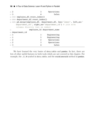
![100 • A Tour of Data Science: Learn R and Python in Parallel
random variable is equal to some value, but PDF does not represent probabilities
directly.
The quantile function is the inverse of CDF, i.e.,
QX(p) = inf{x ∈ R : p ≤ FX(x)}. (4.2)
PDF, CDF and quantile functions are all heavily used in quantitative analysis.
In R and Python, we can find a number of functions to evaluate these functions. The
best known distribution should be univariate normal/Gaussian distribution. Let’s use
Gaussian random variables for illustration.
R
1 > # for reproducibility
2 > set.seed(42)
3 > # draw samples
4 > x = rnorm(10, mean=0, sd=2)
5 > print(x)
6 [1] 2.7419169 −1.1293963 0.7262568 1.2657252 0.8085366
7 [6] −0.2122490 3.0230440 −0.1893181 4.0368474 −0.1254282
8 > print(mean(x))
9 [1] 1.094594
10 > print(sd(x))
11 [1] 1.670898
12 > # evaluate PDF
13 > d = dnorm(x, mean=0, sd=2)
14 > print(d)
15 [1] 0.07793741 0.17007297 0.18674395 0.16327110 0.18381928
16 [6] 0.19835103 0.06364496 0.19857948 0.02601446 0.19907926
17 > # evalute CDF
18 > p = pnorm(x, mean=0, sd=2)
19 > print(p)
20 [1] 0.9148060 0.2861395 0.6417455 0.7365883 0.6569923 0.4577418
21 [7] 0.9346722 0.4622928 0.9782264 0.4749971
22 > # evaluate quantile
23 > q = qnorm(p, mean=0, sd=2)
24 > print(q)
25 [1] 2.7419169 −1.1293963 0.7262568 1.2657252 0.8085366
26 [6] −0.2122490 3.0230440 −0.1893181 4.0368474 −0.1254282
We see that qnorm(pnorm(x)) = x. In Python, we use the functions in numpy and
scipy.stats for the same purpose.
Python](https://image.slidesharecdn.com/a-tour-of-data-science-learn-r-and-python-in-parallel-1st-edition-241027161058-87cda925/85/a-tour-of-data-science-learn-r-and-python-in-parallel-1st-edition-pdf-111-320.jpg)
![Random Variables, Distributions & Linear Regression • 101
1 >>> import scipy.stats
2 >>> import numpy as np
3 >>> import scipy.stats
4 >>> np.random.seed(42)
5 >>> x = np.random.normal(loc=0.0, scale=2.0, size=10)
6 >>> print(x)
7 [ 0.99342831 −0.2765286 1.29537708 3.04605971 −0.46830675
−0.46827391
8 3.15842563 1.53486946 −0.93894877 1.08512009]
9 >>> norm = scipy.stats.norm(loc=0.0, scale=2.0)
10 >>> d = norm.pdf(x)
11 >>> print(d)
12 [0.17632116 0.19757358 0.16172856 0.06254333 0.19407713
0.19407788
13 0.05732363 0.1485901 0.17865677 0.17217026]
14 >>> p = norm.cdf(x)
15 >>> print(p)
16 [0.69030468 0.44501577 0.74140679 0.93612438 0.40743296
0.40743933
17 0.94285637 0.77858846 0.31936529 0.70628362]
18 >>> q = norm.ppf(p) # ppf is the quantile function
19 >>> print(q)
20 [ 0.99342831 −0.2765286 1.29537708 3.04605971 −0.46830675
−0.46827391
21 3.15842563 1.53486946 −0.93894877 1.08512009]
A random variable could also be multivariate. In fact, the univariate normal
distribution is a special case of multivariate normal distribution whose PDF is given
in
1 1
p(x; μ, Σ) = exp(− ( 1
x − μ)T
Σ−
(x − μ
(2 ) 2 Σ 1/2
))
π m/ 2
, (4.3)
| |
where μ is the mean and Σ is the covariance matrix of the random variable x.
Sampling from distributions are involved in many algorithms, such as Monte
Carlo simulation. First, let’s see a simple example in which we draw samples from a
3-dimensional normal distribution.
R Python
1 > library(mvtnorm) 1 >>> from scipy.stats import
2 > mu = c(1, 2) multivariate_normal
array mvn
= ( as
3 > cov
2 >>> mu = np.array([1,2])
c(1.0, 0.5, 0.5, 2.0),
c(2, 2))](https://image.slidesharecdn.com/a-tour-of-data-science-learn-r-and-python-in-parallel-1st-edition-241027161058-87cda925/85/a-tour-of-data-science-learn-r-and-python-in-parallel-1st-edition-pdf-112-320.jpg)
![102 • A Tour of Data Science: Learn R and Python in Parallel
4 > set.seed(42) 3 >>> cov = np.array([[1,
5 > x = rmvnorm(n = 1, 0.5],[0.5, 2]])
mean = mu, sigma = cov) 4 >>> mvn.random_state.seed
6 > print(x)
(42)
7 [,1] [,2]
5 >>> dist = mvn(mean = mu,
8 [1,] 2.221431 1.498778
cov = cov)
9 > d = dmvnorm(x,
6 >>> x = dist.rvs(size=1)
mean = mu, sigma = cov)
7 >>> print(x)
10 > print(d)
[1.16865045 2.72887797]
11 [1] 0.04007949 8
9 >>>
− d = dist.pdf(x)
12 > p = pmvnorm(lower= Inf,
upper = x[1,], 10 >>> print(d)
mean = mu, sigma = cov) 11 0.10533537790438291
13 > print(p)
12 >>> p = dist.cdf(x)
14 [1] 0.344201
13 >>> print(p)
15 attr(,"error")
14 0.44523665187828293
16 [1] 1e 15
17
−
attr(,"msg")
18 [1] "Normal Completion"
Please note in the example above, we do not calculate the quantiles. For multi-
variable distributions, the quantiles are not necessarily fixed points.
4.2 INVERSION SAMPLING & REJECTION SAMPLING
4.2.1 Inversion sampling
Sampling from the Gaussian or other famous distributions could be as simple as just
calling a function. What if we want to draw samples from any distribution with its
CDF? Inversion sampling is a generic solution. The key idea of inversion sampling
is that FX(x) always follows a uniform distribution between 0 and 1. There are two
steps in drawing a sample with the inversion sampling approach.
1. draw independent and identical (i.i.d.) distribution random variables u1, ..., un
which are uniformly distributed from 0 to 1;
2. calculate the quantiles q1, ..., qn for u1, ..., un based on the CDF, and return
q1, ..., qn as the desired samples to draw.
Let’s see how to use the inversion sampling technique to sample from exponential
distribution with CDF f −λx
X(x; λ) = 1 − e .
R Python
1 > n=1000 1 >>> import numpy as np
2 > set.seed(42) 2 >>> np.random.seed(42)
3 > # step 1, draw from 3 >>> n=1000
uniform dist](https://image.slidesharecdn.com/a-tour-of-data-science-learn-r-and-python-in-parallel-1st-edition-241027161058-87cda925/85/a-tour-of-data-science-learn-r-and-python-in-parallel-1st-edition-pdf-113-320.jpg)
![Random Variables, Distributions & Linear Regression • 103
4 > u = runif(n=n, min=0, 4 >>> # step 1, generate from
max=1) uniform(0,1)
5 > # step 2, calculate the 5 ... u = np.random.uniform(
quantiles low=0, high=1, size=n)
6 > lambda = 2.0
6 >>> # step 2, calculate the
7 > x = qexp(u, rate = lambda) quantile
8 > # the mean is close to 1/ 7 ... lamb = 2.0
lambda 8 >>> q = u)/lamb
9 > mean(x)
9
−np.log(1−
>>> np.mean(q)
10 [1] 0.4818323
10 0.4862529739826122
In the above R implementation, we used the built-in quantile function in step
2; however, for many distributions there are no built-in quantile functions available
and thus we need to specify the quantile function ourselves (illustrated in the Python
implementation).
4.2.2 Rejection sampling
Rejection sampling is also a basic algorithm to draw samples for a random variable X
given its PDF fX. The basic idea of rejection sampling is to draw samples for a random
variable Y with PDF fY and accept the samples with probability fX(x)/(MfY (x)).
M is selected such that fX(x)/(MfY (x)) ≤ 1. If the sample generated is rejected,
the sampling procedure is repeated until an acceptance. More theoretical details
of rejection sampling can be found from wikipedia2
. The distribution fY is called
proposal distribution.
Let’s try to draw samples from an exponential distribution truncated between 0
and b. The PDF of this random variable is specified by fX(x; λ, b) = λe−λx
/(1−e−λb
).
A naive approach is to sample from the untruncated exponential distribution and
only accept samples smaller than b, which is implemented as follows.
R Python
1 n=1000 1 import numpy as np
2 set.seed(42) 2 np.random.seed(42)
3 lambda = 1.0 3 lamb, b = 1.0, 2.0
4 b = 2.0 4 n=1000
5 x = rep(0, n) 5 x = []
6 i = 0 6 i = 0
7 while (i<n){ 7 while i<n:
8 y = rexp(n = 1, rate = 8 y = np.random.exponential(
lambda) scale = lamb, size = 1)
9 if (y<=b) { 9 if y<=b:
10 i=i+1 10 x.append(y[0])
11 x[i] = y 11 i+=1
12 }
2
https://en.wikipedia.org/wiki/Rejection_sampling](https://image.slidesharecdn.com/a-tour-of-data-science-learn-r-and-python-in-parallel-1st-edition-241027161058-87cda925/85/a-tour-of-data-science-learn-r-and-python-in-parallel-1st-edition-pdf-114-320.jpg)
![104 • A Tour of Data Science: Learn R and Python in Parallel
13 }
After running the code snippets above, we have the samples stored in x from the
truncated exponential distribution.
Now let’s use the rejection sampling technique for this task. Since we want to
sample the random variable between 0 and b, one natural choice of the proposal
distribution fY is a uniform distribution between 0 and b and we choose M = bλ/(1−
−λx
e−λb
). As a result, the acceptance probability fX(x)/(MfY (x)) becomes e .
R
1 n=1000
2 set.seed(42)
3 lambda = 1.0
4 b = 2.0
5 x = rep(0, n)
6 i = 0
7 while (i<n){
8 # sample from the proposal
distribution
9 y = runif(1, min = 0,
max = b)
10 # calculate the acceptance
probability
11 p = exp(−lambda∗y)
12 if (runif(1)<=p) {
13 i=i+1
14 x[i] = y
15 }
16 }
Python
1 import numpy as np
2 np.random.seed(42)
3 lamb, b = 1.0, 2.0
4 n = 1000
5 x = []
6 i = 0
7 while i < n:
8 # sample from the
proposal distribution
9 y = np.random.uniform(
low=0, high=b)
10 # calculate the
acceptance
probability
11 p = np.exp(−lamb∗y)
12 if p >= np.random.
uniform():
13 x.append(y)
14 i += 1
We have seen the basic examples on how to draw samples with inversion samples
and truncated samples. Now let’s work on a more challenging problem.
Application - Draw samples from a sphere
Without loss of generality, let’s consider a unit sphere, i.e., the radius r = 1. We want to
draw i.i.d. points from a unit sphere.](https://image.slidesharecdn.com/a-tour-of-data-science-learn-r-and-python-in-parallel-1st-edition-241027161058-87cda925/85/a-tour-of-data-science-learn-r-and-python-in-parallel-1st-edition-pdf-115-320.jpg)
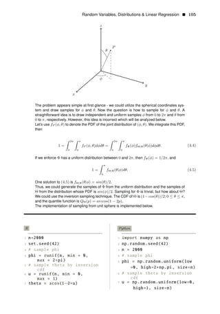

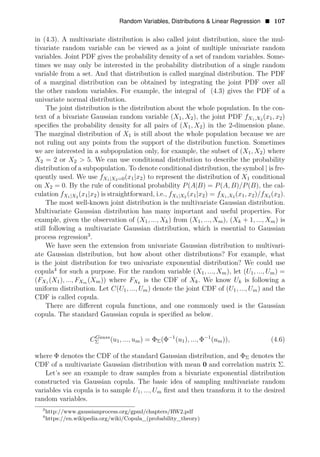
![108 • A Tour of Data Science: Learn R and Python in Parallel
R
1 > library(mvtnorm)
2 > n = 10000
3 > set.seed(42)
4 > rates = c(1.0, 2.0)
5 > mu = c(0, 0)
6 > rho = 0.6
7 > correlation = array(c(1, rho, rho, 1), c(2, 2))
8 > # sample R from multivariate Gaussian
9 > r = rmvnorm(n = n, mean = mu, sigma = correlation)
10 > # generate U
11 > u = pnorm(r)
12 > # calculate the quantile for X
13 > x1 = qexp(u[, 1], rate = rates[1])
14 > x2 = qexp(u[, 2], rate = rates[2])
15 > x = cbind(x1, x2)
16 > cor(x)
17 x1 x2
18 x1 1.0000000 0.5476137
19 x2 0.5476137 1.0000000
20 > apply(x, mean, MARGIN = 2)
21 x1 x2
22 0.9934398 0.4990758
Python
1 >>> import numpy as np
2 >>> from scipy.stats import multivariate_normal as mvn
3 >>> from scipy.stats import norm
4 >>> mu = np.array([0, 0])
5 >>> rho = 0.6
6 >>> cov = np.array([[1, rho],[rho, 1]])
7 >>> mvn.random_state.seed(42)
8 >>> n = 10000
9 >>> uvn = norm(loc=0.0, scale=1.0)
10 >>> dist = mvn(mean = mu, cov = cov)
11 >>> rates = [1.0, 2.0]
12 >>> # sample R from multivariate Gaussian
13 ... r = dist.rvs(size=n)
14 >>> # generate U
15 ... u = uvn.cdf(r)
16 >>> # calculate the quantile for X
17 ... def qexp(u, rate): return −np.log(1−u)/rate
18 ...](https://image.slidesharecdn.com/a-tour-of-data-science-learn-r-and-python-in-parallel-1st-edition-241027161058-87cda925/85/a-tour-of-data-science-learn-r-and-python-in-parallel-1st-edition-pdf-119-320.jpg)
![Random Variables, Distributions & Linear Regression • 109
Figure 4.2: Samples from a bivariate exponential distribution constructed via Gaus
sian copula
19 >>> x1 = qexp(u[:, 0], rate = rates[0])
20 >>> x2 = qexp(u[:, 1], rate = rates[1])
21 >>> x = np.column_stack((x1, x2))
22 >>> np.corrcoef(x.T)
23 array([[1. , 0.57359023],
24 [0.57359023, 1. ]])
25 >>> np.mean(x, axis=0)
26 array([0.99768825, 0.50319692])
We plot 2000 samples generated from the bivariate exponential distribution con
structed via copula in Figure 4.2.
With the help of copula, we can even construct joint distribution with marginals
from different distributions. For example, let’s make a joint distribution of a uniform
distributed random variable and an exponential distributed random variable.
R
1 > library(mvtnorm)
2 > n = 10000
3 > set.seed(42)
4 > mu = c(0, 0)
5 > rho = 0.6
6 > correlation = array(c(1, rho, rho, 1), c(2, 2))
7 > # sample R from multivariate Gaussian
8 > r = rmvnorm(n = n, mean = mu, sigma = correlation)
9 > # generate U
10 > u = pnorm(r)](https://image.slidesharecdn.com/a-tour-of-data-science-learn-r-and-python-in-parallel-1st-edition-241027161058-87cda925/85/a-tour-of-data-science-learn-r-and-python-in-parallel-1st-edition-pdf-120-320.jpg)
![110 • A Tour of Data Science: Learn R and Python in Parallel
Figure 4.3: Samples from a joint distribution of a uniform marginal and an exponential
marginal
11 > # calculate the quantile for X
12 > # X1 ~ exp(1.0); X2 ~ unif(0, 2)
13 > x1 = qexp(u[, 1], rate = 1.0)
14 > x2 = qunif(u[, 2], min = 0, max = 2)
15 > cor(x1, x2)
16 [1] 0.5220363
4.4 FIT A DISTRIBUTION
Statistics is used to solved real-world problems with data. In many cases we may have
a collection of observations for a random variable and want to know the distribution
which the observations follow. In fact, there are two questions involved in the process
of fitting a distribution. First, which distribution to fit? And second, given the distri
bution, how to estimate the parameters. These two questions are essentially the same
questions that we have to answer in supervised learning. In supervised learning, we
need to choose a model and estimate the parameters (if the model has parameters).
We can also refer to these two questions as model selection and model fitting. Usually,
model selection is done based on the model fitting.
Two widely-used methods in distribution fitting are method of moments and the
maximum likelihood method. In this section we will see the method of moments. The
maximum likelihood method will be introduced in Chapter 6. The kth
moment of
a random variable is defined as μk = E(xk
). If there are m parameters, usually we
derive the first m theoretical moments in terms of the parameters, and by equating
n k
these theoretical moments to the sample moments μ̂k = 1/n 1 xi we will get the
estimate.
Let’s take the univariate Gaussian distribution as an example. We want to esti](https://image.slidesharecdn.com/a-tour-of-data-science-learn-r-and-python-in-parallel-1st-edition-241027161058-87cda925/85/a-tour-of-data-science-learn-r-and-python-in-parallel-1st-edition-pdf-121-320.jpg)
![Random Variables, Distributions & Linear Regression • 111
mate the mean μ and variance 2
σ . The first and second theoretical moments are μ and
2 2
μ + σ . Thus, the estimate and 2
μ̂ 2 2
σ̂ are 1/n n n n
1 xi and 1/n 1 xi − (1/n 1 xi) =
1/n n
1 (xi − μ̂)2
. The code snippets below show the implementation.
R Python
1 > set.seed(42) 1 >>> import numpy as np
2 > n = 1000 2 >>> np.random.seed(42)
3 > mu = 2.5 3 >>> n = 1000
4 > var = 1.6 4 >>> mu, var = 2.5, 1.6
5 > x = rnorm(n, mu, 5 >>> x = np.random.normal
sqrt(var)) (2.5, 1.6 0.5, size=n)
6 > mu_est = mean(x)
∗∗
6 >>> mu_est = np.mean(x)
7 > var_est =
7 >>> var_est = np.mean((x
mean((x mu_est)^2)
−
8 > mu_est) 2)
print(mu_est
−
) ∗∗
9 >>> print(mu_est)
[1] 2.467334 8
10 > print(var_est) 9 2.524453331300827
10 >>> print(var_est)
11 [1] 1.60647
11 1.5326479835704276
We could also fit another distribution to the data generated from a normal distri
bution. But which one is better? One answer is to compare the likelihood functions
evaluated at the fitted parameters and choose the one that gives the larger likelihood
value.
Please note that different methods to fit a distribution may lead to different
parameter estimates. For example, the estimate of population variance using the
maximum likelihood method is different from that using the moments method. Ac
tually, the estimator for population mean is biased using the methods method but
the estimator using the maximum likelihood method is unbiased.
4.5 CONFIDENCE INTERVAL
In the previous section we have seen the parameter estimation of a distribution. How
ever, the parameter estimates from either the method of moments or the maximum
likelihood estimation are not the exact values of the unknown parameters. There are
uncertainties associated with distribution fitting because the data to which the dis
tribution is fit usually is just a random sample rather than a population. Suppose
we could repeat the distribution fitting process m times and each time we collect
a random sample of size n (i.e., a collection of n observations for the random vari
able of interest), then we will get n estimates of the distribution parameters. Which
estimate is the best to use? In fact, all these n estimates are observations of the esti
mator random variable. Estimator is a function of the random sample, and itself is a
random variable. For example, eq1 is an estimator for the μ parameter in a Gaussian
distribution.](https://image.slidesharecdn.com/a-tour-of-data-science-learn-r-and-python-in-parallel-1st-edition-241027161058-87cda925/85/a-tour-of-data-science-learn-r-and-python-in-parallel-1st-edition-pdf-122-320.jpg)
![112 • A Tour of Data Science: Learn R and Python in Parallel
4.5.1 Central limit theorem
Now we know when we fit a distribution, the parameter estimates are not the exact
values of the unknown parameters. The question is how to quantify the uncertainties?
To answer this question, we better know the distribution of the estimator. In the
example of the Gaussian distribution, what distribution does the estimator μ̂ follow?
It is straightforward to see that the estimator is still following a Gaussian distribution
since each Xi is following a Gaussian distribution (sum of independent Gaussian
random variables still follows a Gaussian distribution). But what if Xi is from an
arbitrary distribution? We may still derive an exact distribution of the sample mean μ̂
for an arbitrary distribution, but sometimes the derivation may not be easy. A simple
idea is to use the central limit theorem (CLT), which states that the distribution of
the mean of a random sample from a population with finite variance is approximately
√
normally distributed when the sample size is large enough. More specifically, n(X
¯ −
d
μ)/σ −
→ N(0, 1) where μ and σ are the population mean and standard deviation,
respectively. Sometimes we do not have the actual value of the population standard
√
deviation and the sample standard deviation S can be used instead and thus n(X
¯ −
d
μ)/S −
→ N(0, 1).
We know if Z is a Gaussian random variable, P(−Z(1+α)/2 < Z ≤ Z(1+α)/2) = α
√
where Zu denotes the quantile of u. By CLT, P(−Z(1+α)/2 ≤ n(X
¯ − μ)/S ≤
√
Z(1+α)/2) = α, which further leads to P(X
¯ − Z(1+α)/2S/ n ≤ μ ≤ X
¯ +
√ √
¯
Z(1+α)/2S/ n) = α. The interval X ± Z(1+α)/2S/ n is called an α confidence in
terval (CI) for the population mean μ. For example, since Z(1+0.95)/2 = 1.96 the 95%
√
¯
CI is constructed as X
√
± 1.96S/ n. Of course, if we know the exact value of σ, we
could use X
¯ ± 1.96σ/ n instead.
We show an example for the confidence interval calculation of population mean
in normal distribution.
R
1 > set.seed(42)
2 > n = 1000
3 > mu = 2.5
4 > var = 1.6
5 > x = rnorm(n, mu, sqrt(var))
6 > mu_est = mean(x)
7 > # we can also calculate S with sd(x) in R
8 > S = sqrt(sum((x − mu_est) ^ 2) / (n − 1))
9 > alpha = 0.95
10 > Z_alpha = qnorm((1 + alpha) / 2)
11 > CI = c(mu_est − Z_alpha ∗ S / sqrt(n), mu_est + Z_alpha ∗ S /
sqrt(n))
12 > print(CI)
13 [1] 2.388738 2.545931](https://image.slidesharecdn.com/a-tour-of-data-science-learn-r-and-python-in-parallel-1st-edition-241027161058-87cda925/85/a-tour-of-data-science-learn-r-and-python-in-parallel-1st-edition-pdf-123-320.jpg)
![Random Variables, Distributions & Linear Regression • 113
Python
1 >>> import numpy as np
2 >>> import scipy
3 >>> np.random.seed(42)
4 >>> n = 1000
5 >>> mu, var = 2.5, 1.6
6 >>> norm = scipy.stats.norm(loc=0, scale=1)
7 >>> x = np.random.normal(mu, var∗∗0.5, size=n)
8 >>> mu_est = np.mean(x)
9 >>> S = np.sqrt(np.sum((x mu_est) 2)/(n 1))
10
− ∗∗ −
>>> alpha = 0.95
11 >>> Z_alpha = norm.ppf((1+alpha)/2)
12 >>> CI = [mu_est − Z_alpha∗S/np.sqrt(n), mu_est + Z_alpha∗S/np.
sqrt(n)]
13 >>> print(CI)
14 [2.4476842124240363, 2.6012224501776178]
The interpretation of CI is tricky. A 95% CI does not mean the probability that
the constructed CI contains the true population mean is 0.95. Actually, a constructed
CI again is a random variable because the CI is created based on each random
sample collected. Following the classic explanation from textbooks, when we repeat
the procedures to create CI multiple times, the probability that the true parameter
falls into the CI is equal to α. Let’s do an example to see that point.
R
1 > set.seed(42)
2 > B = 1000
3 > n = 1000
4 > mu = 2.5
5 > var = 1.6
6 > alpha = 0.95
7 > Z_alpha = qnorm((1 + alpha) / 2)
8 > coverage = rep(0, B)
9 > for (i in 1:B) {
10 + x = rnorm(n, mu, sqrt(var))
11 + mu_est = mean(x)
12 + S = sqrt(sum((x − mu_est) ^ 2) / (n − 1))
13 + CI = c(mu_est − Z_alpha ∗ S / sqrt(n), mu_est + Z_alpha ∗ S
/ sqrt(n))
14 + coverage[i] = (mu >= CI[1]) && (mu <= CI[2])
15 + }
16 > # the coverage probability should be close to alpha
17 > print(mean(coverage))
18 [1] 0.941](https://image.slidesharecdn.com/a-tour-of-data-science-learn-r-and-python-in-parallel-1st-edition-241027161058-87cda925/85/a-tour-of-data-science-learn-r-and-python-in-parallel-1st-edition-pdf-124-320.jpg)
![114 • A Tour of Data Science: Learn R and Python in Parallel
4.5.2 Bootstrap
So far we have seen how to create the CI for sample mean. What if we are inter
ested in quantifying the uncertainty of other parameters, for example, the variance
of a random variable? If we estimate these parameters with the maximum likelihood
method, we can still construct the CI in a similar approach with the large sample
theory. However, we will not discuss it in this book. Alternatively, we could use the
bootstrap technique.
Bootstrap is simple yet powerful. It is a simulation-based technique. If we want
to estimate a quantity θ, first we write the estimator for θ as a function of a random
sample i.e., θ̂ = g(X1, ..., Xn). Next, we just draw a random sample and calculate
ˆ θ(1)
θ̂(B)
θ and repeat this process B times to get a collection of θ̂ denoted as ˆ , ..., .
From these simulated θ̂, we could simply use the percentile θ̂(1−α)/2 and θ̂(1+α)/2 to
construct the α CI. There are also other variants of the bootstrapping method with
similar ideas.
Let’s try to use bootstrap to construct a 95% CI for the population variance of a
Gaussian distributed random variable.
R
1 > set.seed(42)
2 > B = 1000
3 > n = 1000
4 > mu = 2.5
5 > var = 1.6
6 > alpha = 0.95
7 > Z_alpha = qnorm((1 + alpha) / 2)
8 > var_sample = rep(0, B)
9 > for (i in 1:B) {
10 + x = rnorm(n, mu, sqrt(var))
11 + var_sample[i] = sum((x−mean(x))^2)/(n−1)
12 + }
13 > quantile(var_sample , c((1−alpha)/2, (1+alpha)/2))
14 2.5% 97.5%
15 1.466778 1.738675
4.6 HYPOTHESIS TESTING
We have talked about confidence interval, which is used to quantify the uncertainty
in parameter estimation. The root cause of uncertainty in parameter estimation is
that we do the inference based on random samples. Hypothesis testing is another
technique related to confidence interval calculation.](https://image.slidesharecdn.com/a-tour-of-data-science-learn-r-and-python-in-parallel-1st-edition-241027161058-87cda925/85/a-tour-of-data-science-learn-r-and-python-in-parallel-1st-edition-pdf-125-320.jpg)
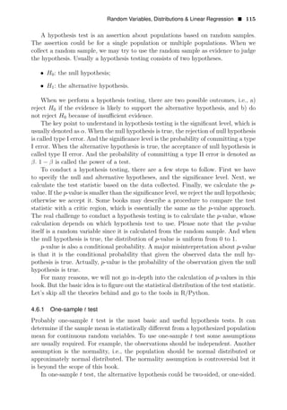
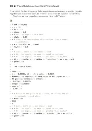
![Random Variables, Distributions & Linear Regression • 117
38 One Sample t−test
39
40 data: x
41 t = −0.21906, df = 49, p−value = 0.5862
42 alternative hypothesis: true mean is greater than 2.5
43 95 percent confidence interval:
44 2.191313 Inf
45 sample estimates:
46 mean of x
47 2.464328
48
49 > # based on the p−value (> alpha), we accept the null
hypothesis stated above
50 > t2$p.value
51 [1] 0.5862418
52 >
53 > # let’s change mu_test and perform a one−sided test again
54 > mu_tes_new = 2.0
55 > t3 = t.test(x, alternative = "greater", mu = mu_tes_new)
56 > print(t3)
57
58 One Sample t−test
59
60 data: x
61 t = 2.8514, df = 49, p−value = 0.003177
62 alternative hypothesis: true mean is greater than 2
63 95 percent confidence interval:
64 2.191313 Inf
65 sample estimates:
66 mean of x
67 2.464328
68
69 > # based on the p−value (< alpha), we reject the null
hypothesis stated above, i.e., we conclude the population
mean is greater than 2.
70 > t3$p.value
71 [1] 0.003177329
Python
1 >>> import numpy as np
2 >>> from scipy.stats import ttest_1samp
3 >>> np.random.seed(42)
4 >>> n = 50](https://image.slidesharecdn.com/a-tour-of-data-science-learn-r-and-python-in-parallel-1st-edition-241027161058-87cda925/85/a-tour-of-data-science-learn-r-and-python-in-parallel-1st-edition-pdf-128-320.jpg)
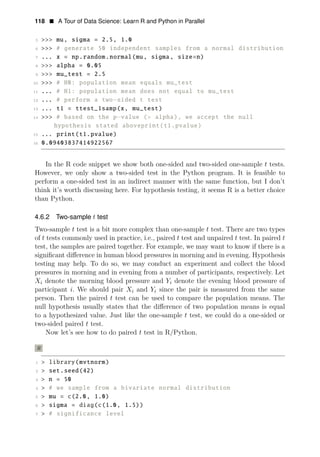
![Random Variables, Distributions & Linear Regression • 119
8 > alpha = 0.95
9 > # sample 50 independent observations from the normal
distribution
10 > mu_diff = 1.2
11 > x = rmvnorm(n, mu, sigma)
12 >
13 > # first, let’s do a two−sided t test
14 > # H0: the population means’ difference is equal to mu_diff
15 > # H1: the population means’ difference is not equal to mu_diff
16 > t.test(x=x[,1], y=x[,2], mu=mu_diff , paired = TRUE,
alternative = "two.sided")
17
18 Paired t−test
19
20 data: x[, 1] and x[, 2]
21 t = −0.86424, df = 49, p−value = 0.3917
22 alternative hypothesis: true difference in means is not equal to
1.2
23 95 percent confidence interval:
24 0.5417625 1.4623353
25 sample estimates:
26 mean of the differences
27 1.002049
28
29 > # we can’t reject H0 based on the fact p value>alpha
30
−
>
31 > # next, let’s do an one−sided t test
32 > # H0: the population means’ difference is equal to mu_diff
33 > # H1: the population means’ difference is less than mu_diff
34 > t.test(x=x[,1], y=x[,2], mu=mu_diff , paired = TRUE,
alternative = "less")
35
36 Paired t−test
37
38 data: x[, 1] and x[, 2]
39 t = −0.86424, df = 49, p−value = 0.1958
40 alternative hypothesis: true difference in means is less than
1.2
41 95 percent confidence interval:
42 −Inf 1.386057
43 sample estimates:
44 mean of the differences
45 1.002049
46
47 > # we can’t reject H0 based on the fact p−value>alpha](https://image.slidesharecdn.com/a-tour-of-data-science-learn-r-and-python-in-parallel-1st-edition-241027161058-87cda925/85/a-tour-of-data-science-learn-r-and-python-in-parallel-1st-edition-pdf-130-320.jpg)
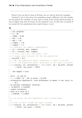
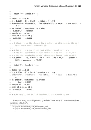
![122 • A Tour of Data Science: Learn R and Python in Parallel
4.7 BASICS OF LINEAR REGRESSION
There are numerous books available on the theory of linear regression, for example,
[9] and [10]. So what is the purpose in writing a few sections about these models
in another book on data science? Many audiences would be interested in how to
implement their own regression models rather than using the off-the-shelf software
packages. By the end of this chapter, we will build up our own linear regression models
in R/Python. We will also see how to reuse some functions in different regressions,
such as linear regression, and those regressions with L2 penalties.
We start from the matrix form of linear regression.
y = Xβ + E, (4.7)
where the column vector y contains n observations on the dependent variable, X is a
n×(p+1) matrix (n > p) of independent variables with constant vector 1 in the first
column, β is a column vector of unknown population parameters to estimate based
on the data, and E is the error term (or noise). For the sake of illustration, (4.7) can
be extended as in
⎡
y1
⎤
1 X11 X21 Xp1 β0 E1
· · ·
⎢
⎢y2
⎥
1 X X X
⎥ 12 22 2 β1 E2
. =
⎡
⎢
⎢
· · ·
.
p
⎤ ⎡ ⎤ ⎡
. . . . +
⎤
⎢
.
⎥ ⎢ . . (4.8)
. . . . .
⎢
.
⎥ ⎢
. . . . .
yn 1 X1n X2n Xpn
⎥
⎥
⎥
⎢
⎢
⎥ ⎢
⎢
.
.
⎥
⎥ ⎢
.
.
⎥
· · · βp
⎥ ⎢
⎢
⎥
⎥
⎥ ⎢
En
⎥
⎣ ⎦ ⎣ ⎦ ⎣ ⎦ ⎣ ⎦
We apply the ordinary least squares (OLS)7
approach to estimate the model pa
rameter β since it requires fewer assumptions than other estimation methods such as
maximum likelihood estimation8
. Suppose the estimated model parameter is denoted
as β̂; we define the residual vector of the system as e = y ˆ
ˆ
− Xβ. The idea of OLS is
to find β which can minimize the sum of squared residuals (SSR), i.e.,
min e1
e (4.9)
β̂
Now the question is how to solve the optimization problem (4.8). First, let’s
expand the SSR.
e1
e = (y − Xβ̂)1
(y ˆ
− Xβ)
(4.10)
= y1
y − 2β̂1
X1
y + β̂1
X1
Xβ̂
The first- and second-order derivatives are calculated as follows
⎧
∂e e
ˆ =
⎨ ˆ
−2X1
y + 2X1
Xβ
∂β
2
∂ e e
(4.11)
= 2X
ˆ
1
X.
∂β∂β̂
⎩
7
https://en.wikipedia.org/wiki/Ordinary_least_squares
8
https://en.wikipedia.org/wiki/Maximum_likelihood_estimation](https://image.slidesharecdn.com/a-tour-of-data-science-learn-r-and-python-in-parallel-1st-edition-241027161058-87cda925/85/a-tour-of-data-science-learn-r-and-python-in-parallel-1st-edition-pdf-133-320.jpg)
![Random Variables, Distributions & Linear Regression • 123
We see that the second-order derivative is positive semidefinite which implies the
SSR in OLS is a convex function (see Section 3.1.4 in [3]) and for an unconstrained
convex optimization problem, the necessary as well as sufficient condition for optimal
ity is that the first-order derivative equals 0 (see Section 4.2.3 in [3]). Optimization
of convex function is very important in machine learning. Actually, the parameter
estimations of many machine learning models are convex optimization problems.
Based on the analysis above, the solution of (4.9) is given in (4.12).
1
β̂ = (X1
X)−
X1
y (4.12)
Now it seems we are ready to write our own linear regression model in R/Python.
The solution in (4.12) involves matrix transportation, multiplication and inversion,
all of which are supported in both R and Python. In Python, we can use the numpy
module for the matrix operations.
However, in practice we don’t solve linear regression with (4.12) directly. Why?
Let’s see an example with
1e + 6 −1
x = .
−1 1e − 6
R
1 > x=array(
c(10^6,−1,−1,10^−6),
c(2,2))
2 > # solve() would return the
inverse matrix
3 > solve(t(x) %∗% x)
4 Error in solve.default(
t(x) %∗% x) :
5 system is computationally
singular: reciprocal
condition number =
2.22044e−28
Python
1 >>> import numpy as np
2 >>> x=np.array([[1e6
,−1],[−1,1e−6]])
3 >>> np.linalg.inv(np.dot(x.
transpose(),x))
4 array([[4.50359963e+03,
4.50359963e+09],
5 [4.50359963e+09,
4.50359963e+15]])
The R code above throws an error because of the singularity of X1
X. It’s in
teresting that the corresponding Python code doesn’t behave in the same way as R,
which has been reported as an issue on github9
.
When the matrix X1
X is singular, how to solve the OLS problem? In this book,
we will focus on the QR decomposition based solution. Singular value decomposition
(SVD) can also be used to solve OLS, which will not be covered in this book.
In linear algebra, a QR decomposition10
of matrix X would factorize X into a
product, i.e., X = QR where Q are orthogonal matrices and R is an upper triangular
matrix. Since the matrix Q is orthogonal (Q1
= Q−1
), we have
9
https://github.com/numpy/numpy/issues/10471
10
https://en.wikipedia.org/wiki/QR_decomposition](https://image.slidesharecdn.com/a-tour-of-data-science-learn-r-and-python-in-parallel-1st-edition-241027161058-87cda925/85/a-tour-of-data-science-learn-r-and-python-in-parallel-1st-edition-pdf-134-320.jpg)
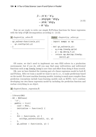
![Random Variables, Distributions & Linear Regression • 125
14 self$coef = qr.coef(qr(x), y)
15 },
16 predict = function(new_x) {
17 cbind(1, new_x) %∗% self$coef
18 }
19 )
20 )
Python chapter4/linear_regression.py
1 import numpy as np
2
3 class LR:
4 def __init__(self):
5 self.coef = None
6
7 def qr_solver(self, x, y):
8 q, r = np.linalg.qr(x)
9 p = np.dot(q.T, y)
10 return np.dot(np.linalg.inv(r), p)
11
12 def fit(self, x, y):
13 self.coef = self.qr_solver(np.hstack((np.ones((x.shape
[0], 1)), x)), y)
14
15 def predict(self, x):
16 return np.dot(np.hstack((np.ones((x.shape[0], 1)), x)),
self.coef)
Now let’s try to use our linear regression model to solve a real regression problem
with the Boston dataset11
, and check the results.
R
1 > source(’linear_regression.R’)
2 >
3 > library(MASS) # load Boston data from this package
4 >
5 > lr = LR$new()
6 > # −i means excluding the ith column from the data.frame
7 > lr$fit(data.matrix(Boston[,−ncol(Boston)]),Boston$medv)
8 > print(lr$coef)
11
https://www.cs.toronto.edu/ delve/data/boston/bostonDetail.html](https://image.slidesharecdn.com/a-tour-of-data-science-learn-r-and-python-in-parallel-1st-edition-241027161058-87cda925/85/a-tour-of-data-science-learn-r-and-python-in-parallel-1st-edition-pdf-136-320.jpg)
![126 • A Tour of Data Science: Learn R and Python in Parallel
9 crim zn indus
chas
10 3.645949e+01 −1.080114e−01 4.642046e−02 2.055863e−02
2.686734e+00
11 nox rm age dis
rad
12 −1.776661e+01 3.809865e+00 6.922246e−04 −1.475567e+00
3.060495e−01
13 tax ptratio black lstat
14 −1.233459e−02 −9.527472e−01 9.311683e−03 −5.247584e−01
15 > # let’s make prediction on the same data
16 > pred=lr$predict(data.matrix(Boston[,−ncol(Boston)]))
17 > print(pred[1:5])
18 [1] 30.00384 25.02556 30.56760 28.60704 27.94352
19 >
20 > # compare it with the R built−in linear regression model
21 > rlm = lm(medv ~ ., data=Boston)
22 > print(rlm$coef)
23 (Intercept) crim zn indus
chas
24 3.645949e+01 −1.080114e−01 4.642046e−02 2.055863e−02
2.686734e+00
25 nox rm age dis
rad
26 −1.776661e+01 3.809865e+00 6.922246e−04 −1.475567e+00
3.060495e 01
27
−
tax ptratio black lstat
28 −1.233459e−02 −9.527472e−01 9.311683e−03 −5.247584e−01
29 > print(rlm$fitted[1:5])
30 1 2 3 4 5
31 30.00384 25.02556 30.56760 28.60704 27.94352
Python
1 >>> from sklearn.datasets import load_boston
2 >>> from linear_regression import LR
3 >>> boston = load_boston()
4 >>> X, y = boston.data, boston.target
5 >>> # first, let’s run our own linear regression
6 ... lr = LR()
7 >>> lr.fit(X, y)
8 >>> print(lr.coef)
9 [ 3.64594884e+01
10
−1.08011358e−01 4.64204584e−02 2.05586264e−02
2.68673382e+00 −1.77666112e+01 3.80986521e+00 6.92224640e−04](https://image.slidesharecdn.com/a-tour-of-data-science-learn-r-and-python-in-parallel-1st-edition-241027161058-87cda925/85/a-tour-of-data-science-learn-r-and-python-in-parallel-1st-edition-pdf-137-320.jpg)
![Random Variables, Distributions & Linear Regression • 127
11 −1.47556685e+00 3.06049479e−01 −1.23345939e−02 −9.52747232e−01
12 9.31168327e−03 −5.24758378e−01]
13 >>> print(lr.predict(X)[:5])
14 [30.00384338 25.02556238 30.56759672 28.60703649 27.94352423]
15 >>>
16 >>> # now, use sklearn’s linear regression model
17 ... from sklearn.linear_model import LinearRegression
18 >>> reg = LinearRegression().fit(X, y)
19 >>> print(reg.coef_)
20 [−1.08011358e−01 4.64204584e−02 2.05586264e−02 2.68673382e+00
21 −1.77666112e+01 3.80986521e+00 6.92224640e−04 −1.47556685e+00
22 3.06049479e−01 −1.23345939e−02 −9.52747232e−01 9.31168327e−03
23 −5.24758378e−01]
24 >>> print(reg.predict(X)[:5])
25 [30.00384338 25.02556238 30.56759672 28.60703649 27.94352423]
The results from our own linear regression models are almost identical to the
results from lm() function or the sklearn.linear_model module, which means we
have done a great job so far.
4.8 RIDGE REGRESSION
What is the problem of solving linear regression model specified by (4.9)? There is
nothing wrong at all with that approach. But I would like to cite my favorite quote —
"Essentially, all models are wrong, but some are useful"12
. (4.9) provides one solution
to model (4.7). There are some alternative solutions, such as lasso regression and
ridge regression. In this section, let’s focus on ridge regression.
What is ridge regression? Ridge regression doesn’t change the model itself. In
stead, it changes the way to estimate model parameters. By naive OLS, we minimize
the SSR directly. In ridge regression, we change the objective function (which is
commonly called loss function in machine learning models) by adding an additional
penalty
1
min e e + λβ1
β. (4.14)
β̂
The optimization problem (4.14) is still an unconstrained optimization problem
and it is convex. It can also be formulated as a constrained convex optimization
problem as
min e1
e
β̂ (4.15)
subject to β1
β ≤ t.
12
https://en.wikipedia.org/wiki/All_models_are_wrong](https://image.slidesharecdn.com/a-tour-of-data-science-learn-r-and-python-in-parallel-1st-edition-241027161058-87cda925/85/a-tour-of-data-science-learn-r-and-python-in-parallel-1st-edition-pdf-138-320.jpg)
![128 • A Tour of Data Science: Learn R and Python in Parallel
The theory behind ridge regression can be found from The Elements of Statistical
Learning [9]. Let’s turn our attention to the implementation of ridge regression. The
solution to (4.15) can be obtained in the same way as the solution to (4.9), i.e.,
ˆ 1
β = (X1
X + λI)−
X1
y. (4.16)
Again, in practice we don’t use (4.16) to implement ridge regression for the same
reasons that we don’t use (4.12) to solve linear regression without penalty.
Actually, we don’t need new techniques to solve (4.14). Let’s make some trans
formation on the objective function in (4.14):
n p
1 2 2
e e + λβ1
β = (yi
i
− x1
iβ) +
√
(0 − λβi) (4.17)
=1 i=1
, where xi = [1, X1i, X2i, ..., Xpi]1
.
Let’s define an augmented dataset:
⎡
1 X11 X21 Xp1 y1
· · ·
⎢ 1 X12 X22 · · · Xp2
⎤ ⎡
y2
⎢
. . . . .
⎤
⎢
. . . . . .
. . . . .
⎢ .
.
⎢
⎥ ⎢
1 X1n X2n · · · X
⎥
⎥
pn
⎥
⎢
⎢
⎥
⎥
Xλ =
⎢
⎢√
λ 0 0 · · · 0
⎥ ⎢ ⎥
√
λ
⎥
⎥
⎥ y
⎢
⎢
⎢ n
, yλ =
⎥
⎥
⎢
⎢ ⎢
0
⎥
⎥
⎥
. (4.18)
⎢
⎥
⎥
⎢
0 0 0
⎢ · · · 0
⎢
0 0
√
⎢
⎢
λ
. . .
· · · 0
⎥ ⎢
0
⎥
⎢
. . . . . .
.. .
⎥
⎥
⎥
⎢
⎢
⎢
⎥
⎥ ⎢
⎢
⎥
⎢
⎢
. . . .
⎥ .
.
⎥
⎥
0 0
√
0 λ 0
⎥
⎥
0
⎥
⎣ ⎦ ⎣
If we regress yλ on Xλ, the OLS solution is just what we are looking
⎦
for. However,
usually the penalty is not applied on the intercept. Thus, we modify yλ and Xλ to
⎡
1 X11 X21 · · · Xp1
1 X12 X22 · · · X
⎤ ⎡
y1
⎢
⎢
.
p2 y2
. . . .
. . . . .
⎥
⎥
⎢
⎢
.
⎤
⎢
. . . . . .
.
1 X1n X2n Xpn
⎥ ⎢
yn
⎥
⎥
⎥
Xλ =
⎢
⎢
⎢
⎢ · · ·
√ = (4.19)
0
⎥
⎥
⎢
⎥
⎥
⎥
⎢
⎢ ⎥
⎢
⎢0
,
λ 0
yλ .
· · · 0
√
⎢
⎢
0 0 λ · · · 0
⎥
⎥ ⎢ ⎥
. . . . .
. . . . .
⎥
⎥
⎢
⎢
0
⎥
⎥
⎢
.
.
⎢
⎢
. . . . .
⎥
⎢
⎢
.
⎥
⎥
0 0 0 0
√
λ
⎥
⎥
⎢
⎢
⎥
⎥ ⎢
0
⎥
⎥
⎣
Now we are ready to implement our own ridge
⎦
regression
⎣
mo
⎦
del based on the
description above. It is also common to normalize13
the independent variables before
applying ridge regression to make different variables in the same order of magnitude.
R chapter4/linear_regression_ridge.R
13
https://en.wikipedia.org/wiki/Normalization_(statistics)](https://image.slidesharecdn.com/a-tour-of-data-science-learn-r-and-python-in-parallel-1st-edition-241027161058-87cda925/85/a-tour-of-data-science-learn-r-and-python-in-parallel-1st-edition-pdf-139-320.jpg)
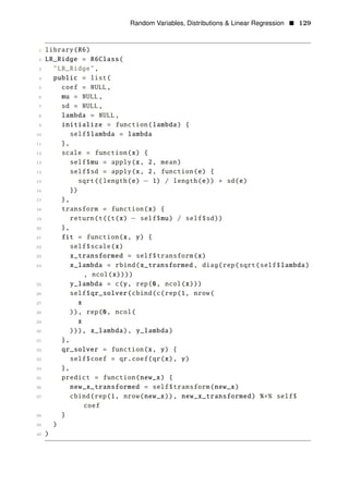
![130 • A Tour of Data Science: Learn R and Python in Parallel
Python chapter4/linear_regression_ridge.py
1 import numpy as np
2 from sklearn.preprocessing import StandardScaler
3
4
5 class LR_Ridge:
6 def __init__(self, l):
7 self.l = l
8 self.coef = None
9 self.scaler = StandardScaler()
10
11 def qr_solver(self, x, y):
12 q, r = np.linalg.qr(x)
13 p = np.dot(q.T, y)
14 return np.dot(np.linalg.inv(r), p)
15
16 def fit(self, x, y):
17 x_transformed = self.scaler.fit_transform(x)
18 x_lambda = np.vstack(
19 (x_transformed , np.diag([self.l∗∗0.5]∗x.shape[1])))
20 x_lambda = np.hstack(
21 (np.vstack((np.ones((x.shape[0], 1)), np.zeros((x.
shape[1], 1)))), x_lambda))
22 y_lambda = np.hstack((y, np.zeros((x.shape[1],))))
23 self.coef = self.qr_solver(x_lambda , y_lambda)
24
25 def predict(self, x):
26 new_x_transformed = self.scaler.transform(x)
27 new_x_transformed = np.hstack(
28 (np.ones((x.shape[0],1)), new_x_transformed)
29 )
30 return np.dot(new_x_transformed , self.coef)
In R, we implement our own scaler; but in the Python implementation, we use
StandardScaler from sklearn.preprocessing module, which is very handy. Please
pay attention to how we calculate the standard deviation14
in R - we are using the
formula of population standard deviation rather than the formula of sample standard
deviation. Actually it doesn’t matter which formula we use to calculate the standard
deviation. I made the choice to use population standard deviation formula in order
to generate consistent result of the StandardScaler since StandardScaler uses the
formula of population standard deviation.
The selection of best λ requires solving the OLS problem repeatedly with different
14
https://en.wikipedia.org/wiki/Standard_deviation](https://image.slidesharecdn.com/a-tour-of-data-science-learn-r-and-python-in-parallel-1st-edition-241027161058-87cda925/85/a-tour-of-data-science-learn-r-and-python-in-parallel-1st-edition-pdf-141-320.jpg)
![Random Variables, Distributions & Linear Regression • 131
values of λ, which implies the QR decomposition procedure would be called multiple
times. Using SVD decomposition could be more efficient in terms of selection of best
λ. But it won’t be covered in the current version of this book.
We are ready to run our own ridge regression on the Boston dataset.
R
1 > source(’linear_regression_ridge.R’)
2 >
3 > library(MASS) # load Boston data from this package
4 >
5 > # let’s try lmabda = 0.5
6 > ridge = LR_Ridge$new(0.5)
7 > ridge$fit(data.matrix(Boston[,−ncol(Boston)]),Boston$medv)
8 > print(ridge$coef)
9 crim zn indus chas
nox
10 22.53280632 −0.92396151 1.07393055 0.12895159 0.68346136
−2.04275750
11 rm age dis rad tax
ptratio
12 2.67854971 0.01627328 −3.09063352 2.62636926 −2.04312573
−2.05646414
13 black lstat
14 0.84905910 −3.73711409
15 > # let’s make prediction on the same data
16 > pred=ridge$predict(data.matrix(Boston[,−ncol(Boston)]))
17 > print(pred[1:5])
18 [1] 30.01652 25.02429 30.56839 28.61521 27.95385
Python
1 >>> from sklearn.datasets import load_boston
2 >>> from linear_regression_ridge import LR_Ridge
3 >>>
4 >>> boston = load_boston()
5 >>> X, y = boston.data, boston.target
6 >>> # first, let’s run our own linear regression
7 ...
8 >>> ridge = LR_Ridge(0.5)
9 >>> ridge.fit(X, y)
10 >>> print(ridge.coef)
11 [ 2.25328063e+01 −9.23961511e−01 1.07393055e+00 1.28951591e−01
12 6.83461360e−01 −2.04275750e+00 2.67854971e+00 1.62732755e−02
13 −3.09063352e+00 2.62636926e+00 −2.04312573e+00 −2.05646414e+00](https://image.slidesharecdn.com/a-tour-of-data-science-learn-r-and-python-in-parallel-1st-edition-241027161058-87cda925/85/a-tour-of-data-science-learn-r-and-python-in-parallel-1st-edition-pdf-142-320.jpg)
![132 • A Tour of Data Science: Learn R and Python in Parallel
14 8.49059103e−01 −3.73711409e+00]
15 >>> print(ridge.predict(X)[:5])
16 [30.01652397 25.02429359 30.56839459 28.61520864 27.95385422]
It’s exciting to see the outputs from R and Python are quite consistent.
Linear regression is not as simple as it seems. To learn more about it, I recommend
reading [10].](https://image.slidesharecdn.com/a-tour-of-data-science-learn-r-and-python-in-parallel-1st-edition-241027161058-87cda925/85/a-tour-of-data-science-learn-r-and-python-in-parallel-1st-edition-pdf-143-320.jpg)
![C H A P T E R 5
Optimization in Practice
We talk about mathematical optimization in this chapter. Mathematical op
timization is the selection of a best element from some set of available
alternatives. Why do we talk about optimization in this book on data science? Data
science is used to help make better decisions, and so is optimization. Operations re
search, with optimization at its core, is a discipline that deals with the application
of advanced analytical methods to make better decisions1
. I always feel data science
and operations research are greatly intertwined. The training of a variety of (super
vised) machine learning models is to minimize the loss functions, which is essentially
an optimization problem. In optimization, the loss functions are usually referred as
objective functions.
Mathematical optimization is a very broad field and we ignore its theories in this
book and only touch some of the simplest applications. Actually, in Chapter 4 we
have seen one of its important applications in linear regression.
5.1 CONVEXITY
The importance of convexity cannot be overestimated. A convex optimization prob
lem [3] has the following form
max f0(x)
x
(5.1)
subject to fi(x) ≤ bi; i = 1, ..., m,
where the vector x ∈ Rn
represents the decision variable; fi; i = 1, ..., m are convex
functions (Rn
→ R). A function fi is convex if
fi(αx + (1 − α)y) ≤ αfi(x) + (1 − α)fi(y), (5.2)
for all x, y ∈ Rn
, and all α ∈ R with 0 ≤ α ≤ 1. (5.1) implies that a convex
optimization problem requires both the objective function and the set of feasible
solutions to be convex. Why do we care about the convexity? Because a convex
optimization problem has a very nice property - a local minimum (which is minimal
1
https://en.wikipedia.org/wiki/Operations_research
133](https://image.slidesharecdn.com/a-tour-of-data-science-learn-r-and-python-in-parallel-1st-edition-241027161058-87cda925/85/a-tour-of-data-science-learn-r-and-python-in-parallel-1st-edition-pdf-144-320.jpg)
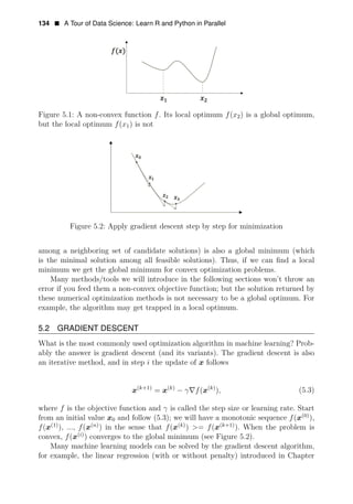
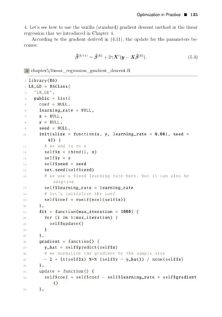
![136 • A Tour of Data Science: Learn R and Python in Parallel
34 predict = function(new_x) {
35 new_x %∗% self$coef
36 }
37 )
38 )
Accordingly, we have the Python implementation as follows.
Python chapter5/linear_regression_gradient_descent.py
1 class LR_GD:
2 """
3 linear regression with vanilla gradient descent
4 """
5
6 def __init__(self, x, y, learning_rate=0.005, seed=42):
7 # we put 1s in the first column of x
8 self.x = np.hstack((np.ones((x.shape[0], 1)), x))
9 self.y = y[:, None]
10 self.seed = seed
11 np.random.seed(self.seed)
12 self.coef = np.random.uniform(size=(self.x.shape[1], 1))
13 self.learning_rate = learning_rate
14
15 def predict(self, new_x):
16 # let’s use @ for matrix multiplication
17 return new_x @ self.coef
18
19 def gradient(self):
20 y_hat = self.predict(self.x)
21 return −2.0∗self.x.T @ (self.y−y_hat)/self.x.shape[0]
22
23 def update(self):
24 self.coef −= self.learning_rate∗self.gradient()
25
26 def fit(self, max_iteration=1000):
27 for _ in range(max_iteration):
28 self.update()
Let’s use simulated dataset to test our algorithm.
R Python
1 > source(’gradient_descent.R 1 >>> from gradient_descent
’) import LR_GD](https://image.slidesharecdn.com/a-tour-of-data-science-learn-r-and-python-in-parallel-1st-edition-241027161058-87cda925/85/a-tour-of-data-science-learn-r-and-python-in-parallel-1st-edition-pdf-147-320.jpg)
![Optimization in Practice • 137
2 > n = 1000 2 >>> import numpy as np
3 > set.seed(42) 3 >>> n = 1000
4 > x = cbind(rnorm(n), 4 >>> np.random.seed(42)
runif(n)) 5 >>> x = np.column_stack((np.
5 > b = 6 # intercept
random.normal(size=n), np
6 > coef = c(2, 3)
.random.uniform(size=n)))
7 > err = runif(n, 0, 0.2)
6 >>> b = 6 # intercept
8 > y = x %∗% coef + b + err
7 >>> coef = np.array([2, 3])
9 > lr_gd = LR_GD
8 >>> err = np.random.uniform(
$new(x = x, y = y,
size=n, low=0, high=0.2)
learning_rate = 0.05)
9 >>> y = x @ coef + b +
10 > lr_gd err
$fit(1000)
,
> >>> lr_gd = LR_GD(x=x y=y,
11 lr_gd$coef 10
learning_rate=0.05)
12 [,1]
13 [1,] it
6.106233 11 >>> lr_gd.f (1000)
rint(lr_gd.coef)
14 2,] >>> p
[ 2.001042 12
15 [3,] 2.992593 13 [[6.09887817]
14 [2.00028507]
15 [2.99996673]]
The results show that our implementation of gradient descent update works well
on the simulated dataset for linear regression.
However, when the loss function is non-differentiable, the vanilla gradient descent
algorithm (4.11) cannot be used. In Chapter 5, we added the 2
L norm (also referred
to as Euclidean norm2
) of β to the loss function to get the ridge regression. What if
we change the 2
L norm to 1
L norm in (4.14)?
p
min e1
e + λ |βi|, (5.5)
β̂ i=1
where λ > 0.
Solving the optimization problem specified in (5.5), we will get the Lasso solution
of linear regression. Lasso is not a specific type of machine learning model. Actually,
Lasso refers to least absolute shrinkage and selection operator. It is a method that
performs both variable selection and regularization. What does variable selection
mean? When we build up a machine learning model, we may collect as many data
points (also called features, or independent variables) as possible. However, if only a
subset of these data points are relevant for the task, we may need to select the subset
explicitly for some reasons. First, it’s possible to reduce the cost (time or money)
to collect/process these irrelevant variables. Second, adding irrelevant variables into
some machine learning models may impact the model performance. But why? Let’s
take linear regression as an example. Including an irrelevant variable into a linear
regression model is usually referred to as model misspecification. (Of course, omitting
a relevant variable also results in a misspecified model.) In theory, the estimator of
2
https://en.wikipedia.org/wiki/Norm_(mathematics)](https://image.slidesharecdn.com/a-tour-of-data-science-learn-r-and-python-in-parallel-1st-edition-241027161058-87cda925/85/a-tour-of-data-science-learn-r-and-python-in-parallel-1st-edition-pdf-148-320.jpg)
![138 • A Tour of Data Science: Learn R and Python in Parallel
coefficients is still unbiased (θ̂ is an unbiased estimator of θ if E(θ̂) = θ) when
an irrelevant variable is included. But in practice, when the irrelevant variable has
non-zero sample correlation coefficient with these relevant variables or the response
variable y, the estimate of coefficient may get changed. In addition, the estimator of
coefficients is inefficient3
. Thus, it’s better to select the relevant variables for a linear
regression.
The Lasso solution is very important in machine learning because of its sparsity,
which results in the automated variable selection. As for why the Lasso solution is
sparse, the theoretical explanation could be found from [9]. Let’s focus on how to solve
it. Apparently, gradient descent algorithm cannot be applied directly to solve (5.5)
although it is still a convex optimization problem since the regularized loss function
is non-differentiable because of ||.
Proximal gradient is one of the algorithms that can be used to solve (5.5) is
called proximal gradient descent [14]. Let’s skip the theory of proximal methods and
the tedious linear algebra, and jump to the solution directly. By proximal gradient
descent, the update is given as follows in each iteration
(k+1)
=
β Sλγ( (
β i)
− 2γ∇(e1
e)))
(5.6)
= Sλγ( (
β i)
+ 2γX1
(y − (
Xβ i)
)),
where Sθ(·) is called soft-thresholding operator given by
zi − θ zi > θ;
[Sθ(z)]i =
⎧
⎪
⎨
0 |zi| ≤ θ; (5.7)
zi + θ zi < −θ.
⎪
⎩
Now we are ready to implement the Lasso solution of linear regression via (5.7).
Similar to ridge regression, we don’t want to put penalty on the intercept, and a
natural estimate of the intercept is the mean of response, i.e., ȳ. The learning rate γ in
each update could be fixed or adapted (change over iterations). In the implementation
below, we use the largest eigenvalue of X1
X as the fixed learning rate.
R chapter5/lasso.R
1 library(R6)
2
3 # soft−thresholding operator
4 sto = function(z, theta){
5 sign(z)∗pmax(abs(z)−rep(theta,length(z)), 0.0)
6 }
7
8 Lasso = R6Class(
9 "LassoLinearRegression",
10 public = list(
3
https://en.wikipedia.org/wiki/Efficient_estimator](https://image.slidesharecdn.com/a-tour-of-data-science-learn-r-and-python-in-parallel-1st-edition-241027161058-87cda925/85/a-tour-of-data-science-learn-r-and-python-in-parallel-1st-edition-pdf-149-320.jpg)
![Optimization in Practice • 139
11 intercept = 0,
12 beta = NULL,
13 lambda = NULL,
14 mu = NULL,
15 sd = NULL,
16 initialize = function(lambda) {
17 self$lambda = lambda
18 },
19 scale = function(x) {
20 self$mu = apply(x, 2, mean)
21 self$sd = apply(x, 2, function(e) {
22 sqrt((length(e)−1) / length(e))∗sd(e)
23 })
24 },
25 transform = function(x) t((t(x) − self$mu) / self$sd),
26 fit = function(x, y, max_iter=100) {
27 if (!is.matrix(x)) x = data.matrix(x)
28 self$scale(x)
29 x_transformed = self$transform(x)
30 self$intercept = mean(y)
31 y_centered = y − self$intercept
32 gamma = 1/(eigen(t(x_transformed) %∗% x_transformed , only.
values=TRUE)$values[1])
33 beta = rep(0, ncol(x))
34 for (i in 1:max_iter){
35 nabla = − t(x_transformed) %∗% (y_centered −
x_transformed %∗% beta)
36 z = beta − 2∗gamma∗nabla
37 print(z)
38 beta = sto(z, self$lambda∗gamma)
39 }
40 self$beta = beta
41 },
42 predict = function(new_x) {
43 if (!is.matrix(new_x)) new_x = data.matrix(new_x)
44 self$transform(new_x) %∗% self$beta + self$intercept
45 }
46 )
47 )
Python chapter5/lasso.py
1
2 import numpy as np](https://image.slidesharecdn.com/a-tour-of-data-science-learn-r-and-python-in-parallel-1st-edition-241027161058-87cda925/85/a-tour-of-data-science-learn-r-and-python-in-parallel-1st-edition-pdf-150-320.jpg)
![140 • A Tour of Data Science: Learn R and Python in Parallel
3 from sklearn.preprocessing import StandardScaler
4
5 def sto(z, theta):
6 return np.sign(z)∗np.maximum(np.abs(z)−np.full(len(z),theta)
, 0.0)
7
8 class Lasso:
9 def __init__(self, l):
10 self.l = l # l is lambda
11 self.intercept = 0.0
12 self.beta = None
13 self.scaler = StandardScaler()
14
15 def fit(self, x, y, max_iter=100):
16 self.intercept = np.mean(y)
17 y_centered = y−self.intercept
18 x_transformed = self.scaler.fit_transform(x)
19 gamma = 1.0/np.linalg.eig(x_transformed.T.dot(
x_transformed))[0].max()
20 beta = np.zeros(x_transformed.shape[1])
21 for _ in range(max_iter):
22 nabla = − np.dot(x_transformed.T, y_centered−np.dot(
x_transformed , beta))
23 z = beta − 2∗gamma∗nabla
24 beta = sto(z, self.l∗gamma)
25 print(z)
26 self.beta = beta
27
28 def predict(self, new_x):
29 new_x_transformed = self.scaler.transform(new_x)
30 return np.dot(new_x_transformed , self.beta) + self.
intercept
Now, let’s see the application of our own Lasso solution of linear regression on
the Boston house-prices dataset.
R
1 > source(’lasso.R’)
2 > library(MASS)
3 > lr = Lasso$new(200)
4 > lr$fit(data.matrix(Boston[,−ncol(Boston)]), Boston$medv, 100)
5 > print(lr$beta)
6 [,1]
7 crim −0.34604592](https://image.slidesharecdn.com/a-tour-of-data-science-learn-r-and-python-in-parallel-1st-edition-241027161058-87cda925/85/a-tour-of-data-science-learn-r-and-python-in-parallel-1st-edition-pdf-151-320.jpg)
![Optimization in Practice • 141
8 zn 0.38537301
9 indus −0.03155016
10 chas 0.61871441
11 nox −1.08927715
12 rm 2.96073304
13 age 0.00000000
14 dis −1.74602943
15 rad 0.02111245
16 tax 0.00000000
17 ptratio −1.77697602
18 black 0.67323937
19 lstat −3.71677103
Python
1 >>> from lasso import Lasso
2 >>> from sklearn.datasets import load_boston
3 >>> boston = load_boston()
4 >>> X, y = boston.data, boston.target
5 >>> lr = Lasso(200.0)
6 >>> lr.fit(X, y, max_iter=100)
7 >>> lr.beta
8 array([−0.34604592, 0.38537301, −0.03155016, 0.61871441,
9
−1.08927715,
2.96073304, −0. , −1.74602943, 0.02111245, −0.
,
10 −1.77697602, 0.67323937, −3.71677103])
In the example above, we set the λ = 200.0 arbitrarily. The results show that the
coefficients of age and tax are zero. In practice, the selection of λ is usually done by
cross-validation which will be introduced later in this book. If you have used the off-
the-shelf Lasso solvers in R/Python you may wonder why the λ used in this example
is so big. One major reason is that in our implementation the first item in the loss
function, i.e., e1
e is not scaled by the number of observations.
In practice, one challenge to apply Lasso regression is the selection of parameter
λ. We will talk about that in Chapter 6 in more detail. The basic idea is to select
the best λ to minimize the prediction error on the unseen data.
5.3 ROOT-FINDING
There is a close relation between optimization and root-finding. To find the roots of
f(x) = 0, we may try to minimize 2
f (x) alternatively. Under specific conditions, to
minimize f(x) we may try to solve the root-finding problem of f1
(x) = 0 (e.g., see](https://image.slidesharecdn.com/a-tour-of-data-science-learn-r-and-python-in-parallel-1st-edition-241027161058-87cda925/85/a-tour-of-data-science-learn-r-and-python-in-parallel-1st-edition-pdf-152-320.jpg)
![142 • A Tour of Data Science: Learn R and Python in Parallel
linear regression in Chapter 5). Various root-finding methods are available in both R
and Python.
Let’s see an application of root-finding in finance.
Application - Internal rate of return
Internal rate of return(IRR) is a measure to estimate an investment’s potential profitability.
In fact, it is a discount rate which makes the net present value (NPV) of all future cashflows
(positive for inflow and negative for outflow) equal to zero. Given the discount rate r, NPV is
calculated as
T
Ci/(1 + r)t
, (5.8)
t=0
where Ci denotes the cashflow and t denotes the duration from time 0. Thus, we can solve
the IRR by finding the root of NPV.
Let’s try to solve IRR in R/Python.
R chapter5/xirr.R
1 NPV = function(cashflow_dates , cashflow_amounts , discount_rate){
2 stopifnot(length(cashflow_dates)==length(cashflow_amounts))
3 days_in_year = 365 # we assume there are 365 days in each year
4 times= as.numeric(difftime(cashflow_dates , cashflow_dates[1],
units="days"))/days_in_year
5 sum(cashflow_amounts/(1.0+discount_rate)^times)
6 }
7 # we name this function as ’xirr’ to follow the convention of MS
Excel
8 xirr = function(cashflow_dates , cashflow_amounts){
9 # we use uniroot function in R for root−finding
10 uniroot(f=function(x) NPV(cashflow_dates ,cashflow_amounts ,x),
interval= c(−1,100))$root
11 }
Python chapter5/xirr.py
1 from datetime import datetime
2 from scipy.optimize import root
3 def NPV(cashflow_dates , cashflow_amounts , discount_rate):
4 assert len(cashflow_dates)==len(cashflow_amounts), "
inconsistent lengths of cashflows dates and amounts"
5 days_in_year=365.0](https://image.slidesharecdn.com/a-tour-of-data-science-learn-r-and-python-in-parallel-1st-edition-241027161058-87cda925/85/a-tour-of-data-science-learn-r-and-python-in-parallel-1st-edition-pdf-153-320.jpg)
![Optimization in Practice • 143
6 times = [(e−cashflow_dates[0]).days/days_in_year for e in
cashflow_dates]
7 return sum(cashflow_amounts[i]/(1.0+discount_rate)∗∗e for i,e
in enumerate(times))
8 def xirr(cashflow_dates , cashflow_amounts):
9 # we use the scipy.optimize.root function to find the root
10 return root(fun=lambda x:NPV(cashflow_dates ,cashflow_amounts ,x
),x0=[0.0]).x
R Python
1 > source(’xirr.R’) 1 >>> from xirr import xirr
2 > cashflow_dates = c( 2 >>> from datetime
as.Date(’2010−01−01’), import datetime
as.Date(’2010 06 01’), 3 >>> cashflow_dates=[datetime
as.Date(’2012
−
01
−
− −01’))
(2010,1,1), datetime
3 > cashflow_amounts =
c(−1000, 200, 1000) (2010,6,1), datetime
4 > xirr(cashflow_dates , (2012,1,1)]
cashflow_amounts) 4 >>> cashflow_amounts=[ 1000,
5 [1] 0.1120706
−
200, 1000]
5 >>> xirr(cashflow_dates ,
cashflow_amounts)
6 array([0.1120734])
Please note the R function uniroot works on one-dimensional functions only,
while scipy.optimize.root function also works on multi-dimensional functions. scipy
.optimize.root requires an initial guess for the solution, but uniroot does not. To
find roots of multi-dimensional functions in R, the optim function introduced in the
next section can also be used. Also, the package rootSolve could be useful. There are
other useful features from both functions; for example, we can control the tolerance
for termination.
5.4 GENERAL PURPOSE MINIMIZATION TOOLS IN R/PYTHON
Implementing our own algorithms from scratch could be fun and may help us better
understand how the algorithms work, but they may not be always efficient and stable.
There are established packages ready to use for many algorithms. For general pur
pose minimization problems, we can use the optim function in R and scipy.optimize
.minimize function in Python as a black box. Various optimization algorithms have
been implemented as the workhorse of these two functions. Some of these optimiza
tion algorithms (e.g., Quasi-Newton methods4
) require the gradients, and some are
derivate-free (e.g., Nelder–Mead method5
). First, let’s see a simple example.
4
https://en.wikipedia.org/wiki/Quasi-Newton_method
5
https://en.wikipedia.org/wiki/Nelder-Mead_method](https://image.slidesharecdn.com/a-tour-of-data-science-learn-r-and-python-in-parallel-1st-edition-241027161058-87cda925/85/a-tour-of-data-science-learn-r-and-python-in-parallel-1st-edition-pdf-154-320.jpg)
![144 • A Tour of Data Science: Learn R and Python in Parallel
Application - Maximum likelihood estimation of normal distribution
Maximum likelihood 6
estimation (MLE) is a very important topic in statistics. I will give a
very brief introduction of what MLE is. To understand MLE, first we need to understand
the likelihood function. Simply speaking, the likelihood function L(θ|x) is a function of the
unknown parameters θ to describe the probability or odds of obtaining the observed data x
(x is a realization of random variable X). For example, when the random variable X follows a
continuous probability distribution with probability density function (pdf) fθ, L(θ|x) = fθ(x).
It’s common to observe a random sample consisting of multiple independent observations
rather than a single observation. In that case, the likelihood function is
n
L(θ|x) = fθ(xi). (5.9)
i=1
Given the observed data and a model on which the data are generated, we may minimize the
corresponding likelihood function to estimate the model parameters. There are some nice
properties of MLE, such as its consistency and efficiency. To better understand MLE and its
properties, I recommend reading [4].
In practice, it’s common to minimize the logarithm of the likelihood function, i.e.,
the log-likelihood function. When X ∼ N(μ, 2
σ ), the pdf of X is given as below
1 ( )2 2 2
f( 2
x|(μ, σ )) = √ e− x−μ / σ
. (5.10)
σ 2π
Taking the logarithm, the log-likelihood function is equal to
n
n 1
L( 2
θ|x) = − log(2π)
2
− n log σ − (
2
xi − μ) .
2 (5.11)
σ i=1
Since the first item in (5.11) is a constant, we can simply set the log-likelihood
function to
1 n
L( 2
θ|x) = −n log σ − (xi − μ) .
2 (5.12)
2σ i=1
It’s worth noting (5.12) is convex. Let’s implement the MLE for normal distribu
tion in R/Python.
R chapter5/normal_mle.R
1 log_lik = function(theta, x){
2 mu = theta[1]
3 sigma = theta[2]
6
https://en.wikipedia.org/wiki/Maximum_likelihood_estimation](https://image.slidesharecdn.com/a-tour-of-data-science-learn-r-and-python-in-parallel-1st-edition-241027161058-87cda925/85/a-tour-of-data-science-learn-r-and-python-in-parallel-1st-edition-pdf-155-320.jpg)
![Optimization in Practice • 145
4 # we return the negative log−likelihood since optim is for
minimization
5 −(−length(x)∗log(sigma) − 0.5/sigma^2∗sum((x−mu)^2))
6 }
7
8 normal_mle = function(x){
9 # par=c(0,1) as the initial values
10 # lower=c(−Inf, 1e−6) for the lower bounds
11 optim(par=c(0, 1), fn=log_lik , x=x, lower=c(−Inf, 1e−6),
method="L−BFGS−B")$par
12 }
Python chapter5/normal_mle.py
1 from scipy.optimize import minimize
2 from numpy.random import normal
3 from math import log
4
5 def log_lik(theta, x):
6 mu = theta[0]
7 sigma = theta[1]
8 # return the negative log−likelihood for minimization
9 return −(−len(x)∗log(sigma) − 0.5/sigma∗∗2∗sum((e−mu)∗∗2 for e
in x))
10
11 def normal_mle(x):
12 return minimize(fun=lambda e:log_lik(e,x),x0=[0,1],method=’L−
BFGS−B’,bounds=((None,None),(1e−6,None))).x
There is no bound set for the mean parameter μ, while we need to set the lower
bound for the standard deviation σ. We chose ’L-BFGS-B’ as the optimization algo
rithm in this example, which requires the gradient of the objective function. When the
gradient function is not provided, the gradient is estimated in the numeric approach.
In general, providing the gradient function may speed up the work. ’L-BFGS-B’ is
a quasi-Newton method. Newton method requires the Hessian matrix for optimiza
tion, but the calculation of Hessian matrix may be expensive or even unavailable
in some cases. The quasi-Newton methods approximate the Hessian matrix of the
objective function instead of calculation. Now let’s use these functions to estimate
the parameters of normal distribution.
R Python
1 > source(’normal_mle.R’) 1 >>> from numpy.random
import seed, normal](https://image.slidesharecdn.com/a-tour-of-data-science-learn-r-and-python-in-parallel-1st-edition-241027161058-87cda925/85/a-tour-of-data-science-learn-r-and-python-in-parallel-1st-edition-pdf-156-320.jpg)
![146 • A Tour of Data Science: Learn R and Python in Parallel
2 > n=100 # generate a random 2 >>> from normal_mle
sample with size = 100 import normal_mle.R
3 > set.seed(42) 3 >>> seed(42)
4 > x=rnorm(n, mean=1.5, 4 >>> n=100
sd=0.8) 5 >>> x=normal(1.5, 0.8, n)
5 > normal_mle(x) 6 >>> normal_mle(x)
6 [1] 1.5260111 0.8289101 7 array([1.41692178,
0.72289325])
Let’s see another application of the general purpose minimization - logistic re
gression.
Application - Logistic regression
We have seen how linear regression works in Chapter 4. Logistic regression works similarly
to linear regression. The major difference is that logistic regression is used in a classification
problem. Classification means to identify to which of a set of categories a new observation
belongs. Among classification problems, if each observation belongs to one of two disjoint
categories, it is a binary classification problem. Binary classification has lots of real-world
applications, such as spam email filter, loan default prediction, and sentiment analysis.
In logistic regression, the prediction output of an observation is the probability that the ob
servation falls into a specific category. Let X represent a n × (p + 1) matrix (n > p) of
independent variables (predictor) with constant vector 1 in the first column, and y repre
sent a column vector of the response variable (target). Please note y is a binary vector, i.e.,
yi ∈ {0, 1}. Formally, a logistic regression is specified as
1
Pr(yi = 1|xi, β) = ,
x
(5.13)
1 + − i
e β
where xi = [1, X1i, X2i, ..., Xpi] , and β denotes the parameter of the logistic model.
What does (5.13) mean? It implies the response variable yi given xi and β follows a
Bernoulli distribution. More specifically, yi ∼ Bern(1/(1 + exp(−xiβ))). Based on the
assumption that the observations are independent, the log-likelihood function is
n
( 1
L β|X, y) = log
(
Pr(yi = 1|xi, β)yi
Pr(y y
i = 0|xi, β) − i
i=1
n
)
=
(
yi log Pr(yi = 1|xi, β) + (1 − yi) log Pr(yi = 0|xi, β)
)
(5.14)
i=1
n
= yixiβ x
− log(1 + e β
i ) .
i=1
( )
Given the log-likelihood function, we can get the maximum likelihood estimate
of logistic regression by minimizing (5.14) which is also convex. The minimization
can be done similarly to linear regression via the iteratively re-weighted least square
method (IRLS) [9]. However, in this section we will not use the IRLS method and](https://image.slidesharecdn.com/a-tour-of-data-science-learn-r-and-python-in-parallel-1st-edition-241027161058-87cda925/85/a-tour-of-data-science-learn-r-and-python-in-parallel-1st-edition-pdf-157-320.jpg)
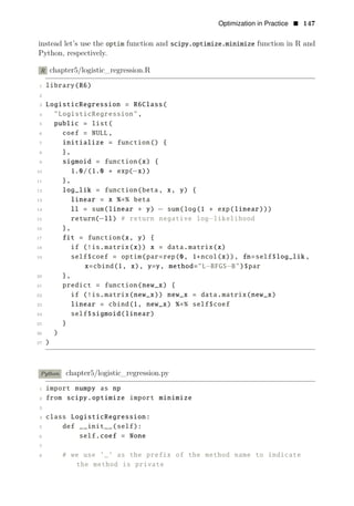
![148 • A Tour of Data Science: Learn R and Python in Parallel
9 def _sigmoid(self, x):
10 return 1.0/(1 + np.exp(−x))
11
12 def _log_lik(self, beta, x, y):
13 linear = np.dot(x, beta)
14 ll = np.sum(linear.dot(y)) − np.sum(np.log(1.0+np.exp(
linear)))
15 return −ll
16
17 def fit(self, x, y):
18 self.coef = minimize(fun=self._log_lik , args=(np.insert(
x, 0, 1.0, axis=1),y), method=’L−BFGS−B’, x0=np.
zeros(1+x.shape[1])).x
19
20 def predict(self, new_x):
21 linear = np.insert(new_x, 0, 1.0, axis=1) # add 1 to
new_x
22 return self._sigmoid(linear)
Now let’s see how to use our own logistic regression. We use the banknote dataset7
in this example. In the banknote dataset, there are four different predictors extracted
from the image of a banknote, which are used to predict if a banknote is genuine or
forged.
R
1 > library(Metrics)
2 > banknote_data = read.csv(’data_banknote_authentication.txt’,
header = FALSE)
3 > colnames(banknote_data) = c(’variance’, ’skewness’, ’curtosis’
, ’entropy’, ’class’)
4 >
5 > lr=LogisticRegression$new()
6 > lr$fit(banknote_data[,1:4], banknote_data$class)
7 > print(lr$coef)
8 [1] 7.3216635 −7.8590497 −4.1907866 −5.2872185 −0.6052346
9 > print(lr$predict(banknote_data[,1:4])[1:5]) # see the first 5
predictions
10 [1] 4.071505e−19 6.741755e 22 2.187781e 10 1.604733e 16
11
− − −
[5] 4.579230e−01
Python
7
https://archive.ics.uci.edu/ml/datasets/banknote+authentication](https://image.slidesharecdn.com/a-tour-of-data-science-learn-r-and-python-in-parallel-1st-edition-241027161058-87cda925/85/a-tour-of-data-science-learn-r-and-python-in-parallel-1st-edition-pdf-159-320.jpg)
![Optimization in Practice • 149
1 >>> from sklearn.metrics import log_loss
2 >>> from logistic_regression import LogisticRegression
3 >>> banknote_data=pd.read_csv(’data_banknote_authentication.txt’
,header=None)
4 >>> from logistic_regression import LogisticRegression
5 >>> lr=LogisticRegression()
6 >>> lr.fit(banknote_data.iloc[:,0:4].values ,banknote_data.iloc
[:,4])
7 >>> print(lr.coef)
8 [ 7.32157876 −7.8591774 −4.19090781 −5.28734934 −0.60536929]
9 >>> lr.predict(banknote_data.iloc[:,0:4].values)[:5] # predict
the probabilities of y=1
10 array([4.06674238e−19, 6.73409431e−22, 2.18663270e−10,
1.60365564e−16,
11 4.57910123e−01])
The above implementation of logistic regression works well. But it is only a ped
agogical toy to illustrate what a logistic regression is and how it can be solved with
general purpose optimization tool. In practice, there are fast and stable off-the-shelf
software tools to choose. It’s also worth noting most of the iterative optimization
algorithms allow to specify the max number of iterations as well as the tolerance.
Sometimes it’s helpful to tune these parameters.
In practice, the penalized ( 1 2
L , L ) versions of logistic regression are more com
monly used than the vanilla logistic regression we introduced above.
5.5 LINEAR PROGRAMMING
In linear programming (LP)8
both the objective function and the constraints are
linear. LP can be expressed as follows,
max c1
x
x
(5.15)
subject to Ax ≤ b,
where the vector x represents the decision variable; A is a matrix, b and c are vectors.
We can do minimization instead of maximization in practice. Also, it’s completely
valid to have equality constraints for LP problems. All LP problems can be con
verted into the form of (5.15). For example, the equality constraint Cx = d can be
transformed to inequality constraints Cx ≤ d and −Cx ≤ −d.
Every LP problem falls into three categories:
1. infeasible - no solution that satisfies all constraints exists;
8
https://en.wikipedia.org/wiki/Linear_programming](https://image.slidesharecdn.com/a-tour-of-data-science-learn-r-and-python-in-parallel-1st-edition-241027161058-87cda925/85/a-tour-of-data-science-learn-r-and-python-in-parallel-1st-edition-pdf-160-320.jpg)
![150 • A Tour of Data Science: Learn R and Python in Parallel
Table 5.1: Available investment opportunities
investment vintage maturity rate of return (annualized)
A year 1 year 2 0.08
B year 2 year 5 0.12
C year 3 year 5 0.16
D year 1 year 4 0.14
2. unbounded - for every feasible solution, there exists another feasible solution
that improves the objective function;
3. having an optimal solution - a unique maximum (or minimum) value of the
objective function exists.
When an LP problem has an optimal solution, there might be different sets of
decision variables that lead to the same optimal value of the objective function. LP
problems are also convex problems [3]. The algorithms to solve LP problems have
been well-studied. The basic and popular algorithm is Dantzig’s simplex method
which was invented in 1947 [7]. More recent interior point methods have better worst-
case complexity than the simplex method. In R/Python, we can find packages that
implement both algorithms.
LP has been extensively used in business, economics, and some engineering prob
lems. First, let’s see a simple application of LP in regression analysis.
Application - Portfolio construction
Let’s assume there are 4 different investment opportunities, A, B, C, and D, listed in Table ??.
There is no intermediate payment between the vintage year and the maturity year. Payments
received on maturity can be reinvested. We also assume the risk-free rate is 0. The goal is
to construct a portfolio using these investment opportunities with $10,000 at year 1 so that
the net asset value at year 5 is maximized.
Let x1, x2, x3 and x4 denote the amount to invest in each investment opportunity; and let
x0 denote the cash not invested in year 1. The problem can be formulated as
max + (1 + 0 08) + (1 + 0 12)3
+ (1 + 0 16)2
+ (1 + 0 14)3
x0 x1 . −x2 − x3 x2 . x3 . x4 .
x
subject to x0 + x1 + x4 = 10000; (5.16)
x0 + x1(1 + 0.08) ≥ x2 + x3;
xi ≥ 0; i = 0, ..., 4.
In Python, there are quite a few tools that can be used to solve LP, such as](https://image.slidesharecdn.com/a-tour-of-data-science-learn-r-and-python-in-parallel-1st-edition-241027161058-87cda925/85/a-tour-of-data-science-learn-r-and-python-in-parallel-1st-edition-pdf-161-320.jpg)
![Optimization in Practice • 151
9
ortools , 10
scipy.optimize.linprog , and 11
CVXPY . We will show the solution using
12
in Python and
ortools lpSolve in R.
R chapter5/portfolio_construction.R
1 library(lpSolve)
2
3 total = 10000.0
4 rate_of_return = c(0, 0.08, 0.12, 0.16, 0.14)
5 # define the objective function
6 f.obj = c(1, 1+rate_of_return[2], −1+(1+rate_of_return[3])^3,
−1+(1+rate_of_return[4])^2, (1+rate_of_return[5])^3)
7 # define the constraints
8 f.con = t(array(c(1, 1, 0, 0, 1, 1, 1+rate_of_return[2], −1, −1,
0), c(5, 2)))
9 # define the direction in the constraints
10 f.dir = c("=", ">=")
11 # define the right hand side of the constraints
12 f.rhs = c(total, 0)
13
14 solution = lp("max", f.obj, f.con, f.dir, f.rhs)
15 cat(’x:’, solution$solution , ’n’)
16 cat(’obj:’, solution$objval , ’n’)
Python chapter5/portfolio_construction.py
1 from ortools.linear_solver import pywraplp
2
3 total = 10000.0
4 rate_of_return = [0.0, 0.08, 0.12, 0.16, 0.14]
5 solver=pywraplp.Solver(’PortfolioConstruction’,pywraplp.Solver.
GLOP_LINEAR_PROGRAMMING)
6
7 # create the variables
8 x=[None]∗5
9 for i in range(5):
10 x[i]=solver.NumVar(0.0, solver.infinity(), ’x’+str(i))
11
12 # create the constraints
13 constraints = [None]∗2
14 # set the equality constraint
9
https://developers.google.com/optimization/
10
https://scipy.org/
11
https://www.cvxpy.org/
12
https://cran.r-project.org/web/packages/lpSolve/lpSolve.pdf](https://image.slidesharecdn.com/a-tour-of-data-science-learn-r-and-python-in-parallel-1st-edition-241027161058-87cda925/85/a-tour-of-data-science-learn-r-and-python-in-parallel-1st-edition-pdf-162-320.jpg)
![152 • A Tour of Data Science: Learn R and Python in Parallel
15 constraints[0] = solver.Constraint(total, total)
16 constraints[0].SetCoefficient(x[0], 1.0)
17 constraints[0].SetCoefficient(x[1], 1.0)
18 constraints[0].SetCoefficient(x[4], 1.0)
19 # set the inequality constraint
20 constraints[1] = solver.Constraint(0.0, solver.infinity())
21 constraints[1].SetCoefficient(x[0], 1.0)
22 constraints[1].SetCoefficient(x[1], 1.0+rate_of_return[1])
23 constraints[1].SetCoefficient(x[2], −1.0)
24 constraints[1].SetCoefficient(x[3], −1.0)
25
26 # set objective function
27 objective = solver.Objective()
28 objective.SetCoefficient(x[0], 1.0)
29 objective.SetCoefficient(x[1], 1.0+rate_of_return[1])
30 objective.SetCoefficient(x[2], −1.0+(1+rate_of_return[2])∗∗3)
31 objective.SetCoefficient(x[3], −1.0+(1+rate_of_return[3])∗∗2)
32 objective.SetCoefficient(x[4], (1+rate_of_return[4]) 3)
33
∗∗
# we want to maximize the objective function
34 objective.SetMaximization()
35 status = solver.Solve()
36 if status == solver.OPTIMAL:
37 sol = [e.solution_value() for e in x]
38 print("x: {0}".format(sol))
39 print("objective: {0}".format(objective.Value()))
Now let’s run our code to get the results.
R Python
1 > source(’ 1 chapter5 $python3.7
portfolio_construction.R portfolio_construction.py
’)
2 x: [0.0, 10800.0,
x: 0 10000.0,
10000 10800 0 0 2
0.0,
3 obj: 15173.22 0.0]
3 objective:
15173.222400000004
We see that the optimal portfolio allocation results in a net asset value of 15173.22
in year 5. You may notice that the Python solution is lengthy compared to the R
solution. That is because the ortools interface in Python is in an OOP fashion and
we add the constraint one by one. But for lpSolve, we utilize the compact matrix
form (5.15) to specify an LP problem. In ortools, we specify the bounds of a decision
variable during its declaration. In lpSolve, all decisions are non-negative by default.
LP also has applications in machine learning; for example, least absolute devia](https://image.slidesharecdn.com/a-tour-of-data-science-learn-r-and-python-in-parallel-1st-edition-241027161058-87cda925/85/a-tour-of-data-science-learn-r-and-python-in-parallel-1st-edition-pdf-163-320.jpg)
![Optimization in Practice • 153
tions (LAD) regression13
can be solved by LP. LAD regression is just another type
of linear regression. The major difference between LAD regression and the linear re
gression we introduced in Chapter 4 is that the loss function to minimize in LAD is
the sum of the absolute values of the residuals rather than the SSR loss.
5.6 MISCELLANEOUS
5.6.1 Stochasticity
The update schedule of gradient descent is straightforward. But what to do if the
dataset is too big to fit into memory? That is a valid question, especially in the era
of big data. There is a naive and brilliant solution - we can take a random sample
from all the observations and only evaluate the loss function on the random sample in
each iteration. Actually, this variant of gradient descent algorithm is called stochastic
gradient descent.
5.6.2 Coordinate descent
You may wonder that if we can randomly take a subset from all the observations,
can we also just take a subset of the variables x? Yes, and sometimes it is quite
useful. For example, in coordinate descent, in each iteration we can update a single
coordinate xj
rather than the entire x. Coordinate descent has been widely applied
for the Lasso solution of the generalized linear models [8].
5.6.3 Newton method
Newton method looks similar to gradient descent, but it requires the Hessian matrix
of the objective function (see (5.17)). In theory, the convergence of Newton method
is faster than the gradient descent algorithm. But not all differentiable objective
functions have second-order derivatives; and the evaluation of Hessian matrix may
also be computationally expensive.
(k+1)
x = (
x k) (k)
)
−1
γH(x f( (
x k)
) (5.17)
− ∇
We have seen the proximal gradient descent method for Lasso. Actually, the
second-order derivatives can also be incorporated into the proximal gradient descent
method, which leads to the proximal Newton method.
5.6.4 Constrained optimization
In general, constrained optimization has the following form.
max f(x)
x
subject to gi(x) ≤ bi; i = 1, ..., m, (5.18)
hi(x) = cj; j = 1, ..., k,
13
https://en.wikipedia.org/wiki/Least_absolute_deviations](https://image.slidesharecdn.com/a-tour-of-data-science-learn-r-and-python-in-parallel-1st-edition-241027161058-87cda925/85/a-tour-of-data-science-learn-r-and-python-in-parallel-1st-edition-pdf-164-320.jpg)
![154 • A Tour of Data Science: Learn R and Python in Parallel
where gi is the inequality constraint and hi is the equality constraint, both of which
could be linear or nonlinear. A constrained optimization problem may or may not
be convex. Although there are some tools existing in R/Python for constrained op
timization, they may fail if you just throw the problem into the tools. It is better
to understand the very basic theories for constrained optimization problems, such as
the Lagrangian, and the Karush-Kuhn-Tucker (KKT) conditions [3].
5.6.5 Quadratic programming
Quadratic programming (QP)14
is also commonly seen in machine learning. For ex
ample, the optimization problems in vanilla linear regression, ridge linear regression
and Lasso solution of linear regression all fall into the QP category. To see why the
Lasso solution of linear regression is also QP, let’s convert the optimization problem
from the unconstrained form (5.5) to the constrained form (5.19) similar to the ridge
regression.
min e1
e
β̂
p (5.19)
subject to λ |βi| ≤ t.
i=1
The || operator in the constraint in (5.19) can be eliminated by expanding the
constraint to 2p
linear constraints.
min e1
e
β̂
subject to
λβ1 + λβ2 + ...+λβn ≤ t (5.20)
−λβ1 + λβ2 + ...+λβn ≤ t
...
λβ1 λβ2 ... λβn t.
− − − − ≤
It is clear the problem specified in (5.20) is a QP problem. The optimization of
support vector machine (SVM) can also be formulated as a QP problem.
In R and Python, there are solvers15
designed specifically for QP problems, which
can be used as a black box.
5.6.6 Metaheuristic optimization
Some optimization algorithms are specific to problems. For example, simplex method
is mostly used for linear programming problems. In contrast, metaheuristic opti
mization algorithms are not problem-specific. Actually, metaheuristic algorithms are
14
https://en.wikipedia.org/wiki/Quadratic_programming
15
https://cran.r-project.org/web/views/Optimization.html, https://cvxopt.org](https://image.slidesharecdn.com/a-tour-of-data-science-learn-r-and-python-in-parallel-1st-edition-241027161058-87cda925/85/a-tour-of-data-science-learn-r-and-python-in-parallel-1st-edition-pdf-165-320.jpg)
![Optimization in Practice • 155
strategies to guide the search process for the solutions. There is a wide variety of meta
heuristic algorithms in the literature, and one of my favorites is simulated annealing
(SA) [16]. SA algorithm can be used for both continuous and discrete optimization
problems (or hybrid, such as mixed integer programming16
). The optim function in R
has the SA algorithm implemented (set method = ’SANN’) for general purpose min
imization with continuous variables. For discrete optimization problems, it usually
requires customized implementation. The pseudocode of SA is given as follows.
• define the cooling schedule Tk, an energy function E, and initial solution s0
• for k = 1, ..., m
– pick a random neighbor sk based on sk−1
– calculate the energy change δ = E(sk) − E(sk−1)
– calculate the acceptance probability P = e−δ/Tk
– if P < random(0, 1), sk = sk−1
• return sm.
Let’s see how we can apply SA for the famous traveling salesman problem.
Application - Traveling salesman problem
Given a list of cities, what is the shortest route that visits each city once and returns to
the original city? This combinatorial optimization problem is the traveling salesman problem
(TSP). When there are K cities, the number of feasible solutions is equal to (K − 1)!/2. It
is difficult to enumerate and evaluate all solutions for a large number of cities. SA algorithm
fits this problem quite well.
Let’s consider a problem with only 10 cities. To apply the SA algorithm, we need to determine
a cooling schedule. For simplicity, we chose Tk = T0αk
. As for the energy function, the
length of the route is a natural choice. For many problems, the challenge to apply SA is how
to generate new solutions from the incumbent. And most of the time there are various ways
to do that, but some may not be efficient. In this TSP problem, we adopt a simple strategy,
i.e., randomly select two different cities from the current route and switch them. If the switch
results in a shorter route we would accept the switch; if the new route is longer, we still could
accept the switch with the acceptance probability.
The implementation of SA with this simple strategy is implemented in both
R/Python as follows.
R chapter5/TSP.R
1 library(R6)
2
3 TSP = R6Class(
16
https://en.wikipedia.org/wiki/Integer_programming](https://image.slidesharecdn.com/a-tour-of-data-science-learn-r-and-python-in-parallel-1st-edition-241027161058-87cda925/85/a-tour-of-data-science-learn-r-and-python-in-parallel-1st-edition-pdf-166-320.jpg)
![156 • A Tour of Data Science: Learn R and Python in Parallel
Figure 5.3: TSP with 10 cities represented by blue dots
4 "TSP",
5 public = list(
6 cities = NULL,
7 distance = NULL,
8 initialize = function(cities, seed = 42) {
9 set.seed(seed)
10 self$cities = cities
11 self$distance = as.matrix(dist(cities))
12 },
13 calculate_length = function(path) {
14 l = 0.0
15 for (i in 2:length(path)) l = l+self$distance[path[i−1],
path[i]]
16 l + self$distance[path[1],path[length(path)]]
17 },
18 accept = function(T_k, energy_old , energy_new) {
19 delta = energy_new − energy_old
20 p = exp(−delta/T_k)
21 p>=runif(1)
22 },
23 solve = function(T_0, alpha, max_iter) {
24 T_k = T_0
25 # create the initial solution s0
26 s = sample(nrow(self$distance), nrow(self$distance),
replace=FALSE)
27 length_old = self$calculate_length(s)
28 for (i in 1:max_iter){](https://image.slidesharecdn.com/a-tour-of-data-science-learn-r-and-python-in-parallel-1st-edition-241027161058-87cda925/85/a-tour-of-data-science-learn-r-and-python-in-parallel-1st-edition-pdf-167-320.jpg)
![Optimization in Practice • 157
29 T_k = T_k∗alpha
30 # we randomly exchange 2 cities in the route
31 candidates = sample(nrow(self$distance), 2, replace=
FALSE)
32 temp = s[candidates[1]]
33 s[candidates[1]] = s[candidates[2]]
34 s[candidates[2]] = temp
35 length_new = self$calculate_length(s)
36 # check if we accept or reject the exchange
37 if (self$accept(T_k, length_old , length_new)){
38 # accept
39 length_old = length_new
40 }else{
41 # reject
42 s[candidates[2]] = s[candidates[1]]
43 s[candidates[1]] = temp
44 }
45 }
46 if (s[1]==1) return(list(’s’=s,’length’=length_old))
47 start = which(s==1)
48 s_reordered = c(s[start:length(s)], s[1:start−1])
49 list(’s’=s_reordered ,’length’=length_old)
50 }
51 )
52 )
Python chapter5/TSP.py
1 import numpy as np
2 from scipy.spatial.distance import cdist
3
4 class TSP:
5 def __init__(self, cities, seed=42):
6 np.random.seed(seed)
7 self.cities = cities
8 # let’s calculate the pairwise distance
9 self.distance = cdist(cities, cities)
10
11 def calculate_length(self, path):
12 l = 0.0
13 for i in range(1, len(path)):
14 l += self.distance[path[i−1], path[i]]
15 return l + self.distance[path[−1], path[0]]
16](https://image.slidesharecdn.com/a-tour-of-data-science-learn-r-and-python-in-parallel-1st-edition-241027161058-87cda925/85/a-tour-of-data-science-learn-r-and-python-in-parallel-1st-edition-pdf-168-320.jpg)
![158 • A Tour of Data Science: Learn R and Python in Parallel
17 def accept(self, T_k, energy_old , energy_new):
18 delta = energy_new − energy_old
19 p = np.exp(−delta/T_k)
20 return p >= np.random.uniform(low=0.0, high=1.0, size=1)
[0]
21
22 def solve(self, T_0, alpha, max_iter):
23 T_k = T_0
24 # let’s create an initial solution s0
25 s = np.random.permutation(len(self.cities))
26 length_old = self.calculate_length(s)
27 for i in range(max_iter):
28 T_k ∗= alpha
29 # we randomly choose 2 cities and exchange their
positions in the route
30 pos_1, pos_2 = np.random.choice(len(s), 2, replace=
False)
31 s[pos_1], s[pos_2] = s[pos_2], s[pos_1]
32 length_new = self.calculate_length(s)
33 # check if we want to accept the new solution or not
34 if self.accept(T_k, length_old , length_new):
35 # we accept the solution and update the old
energy
36 length_old = length_new
37 else:
38 # we reject the solution and reverse the switch
39 s[pos_1], s[pos_2] = s[pos_2], s[pos_1]
40 # let’s reorder the result
41 if s[0] == 0:
42 return s, length_old
43 start = np.argwhere(s == 0)[0, 0]
44 return np.hstack((s[start:], s[:start])), length_old
Let’s run our TSP solver to see the results.
R Python
1 > cities = read.csv(’ 1 >>> from TSP import TSP
chapter5/cities.csv’) 2 >>> cities = pd.read_csv(’
2 > cities = cities[,c(’x’,’y chapter5/cities.csv’)
’)] 3 >>> cities = list(
3 > tsp = TSP$new(cities) zip(cities.x, cities.y))
4 > tsp$solve(2000,0.99,2000) 4 >>> tsp = TSP(cities)
5 $s 5 >>> tsp.solve(2000, 0.99,
6 [1] 1 3 2 10 5 6 9 4 2000)
7 8 6 (array([1, 2, 0, 7, 6, 3, 8,](https://image.slidesharecdn.com/a-tour-of-data-science-learn-r-and-python-in-parallel-1st-edition-241027161058-87cda925/85/a-tour-of-data-science-learn-r-and-python-in-parallel-1st-edition-pdf-169-320.jpg)
![Optimization in Practice • 159
Figure 5.4: Route found by our TSP solver
7 5, 4, 9]),
8 $length 47.372551972154646)
9 [1] 47.37255
In the implementation above, we set the initial temperature to 2000, the cooling
rate α to 0.99. After 2000 iterations, we get the same routes from both implementa
tions. In practice, it’s common to see metaheuristic algorithms get trapped in local
optimums.](https://image.slidesharecdn.com/a-tour-of-data-science-learn-r-and-python-in-parallel-1st-edition-241027161058-87cda925/85/a-tour-of-data-science-learn-r-and-python-in-parallel-1st-edition-pdf-170-320.jpg)

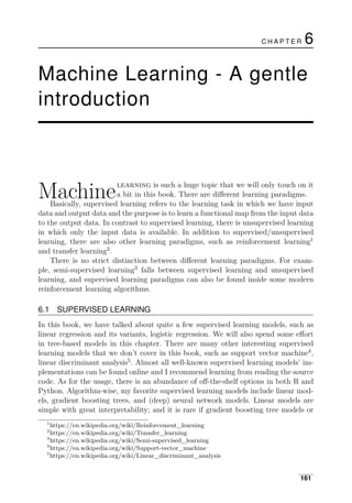
![162 • A Tour of Data Science: Learn R and Python in Parallel
deep neural network models cannot match the prediction accuracy of other models
for a specific problem.
6.1.1 Population & random sample
A population is a complete set of elements of interest for a specific problem. It is
usually defined by the researcher of the problem. A population can be either finite
or infinite. For example, if we define the set of real numbers as our population, it is
infinite. But if we are only interested in the integers between 1 and 100, then we get
a finite population.
A random sample is a set of elements selected from a population. The size of a
random sample could be larger than the population since an element can be taken
multiple times. Why do we care about random samples? Because we are interested
in the population from which the random sample is taken, and the random sample
could help to make inference on the population.
In supervised learning, each element in the population has a set of attributes
which are usually called features or covariates, as well as a label. For example, a
bank may use the mortgage applicant’s personal information (FICO score, years of
employment, debt to income ratio, etc.) as the covariates, and the status of the
mortgage (default, or paid off) as the label. A model can be used to predict the final
status of the mortgage for a new applicant, and such kinds of models are classification
models. When a mortgage is in default status, the applicant may have already made
payments partially. Thus, a model to predict the amount of loss for the bank is also
useful, and such kinds of models are regression models.
But why do we need supervised learning? If we know the labels of the entire
population, nothing is needed to learn. All we need is a database table or a dictionary
(HashMap) for lookup. The issue is that many problems in the real world don’t allow
us to have the labels of the entire population. And thus, we need to learn or infer
based on the random sample collected from the unknown population.
6.1.2 Universal approximation
The universal approximation theorem says that a single hidden layer neural network
can approximate any continuous functions (Rn
→ R) with sufficient number of
neurons under mild assumptions on the activation function (for example, the sigmoid
activation function) [1]. There are also other universal approximators, such as the
decision trees.
Not all machine learning models can approximate universally, for example, the
linear regression without polynomial items. If we have the data from the entire pop
ulation, we may fit the population with a universal approximator. But as we have
discussed earlier, when the entire population is available there is no need to fit a
machine learning model for prediction. But if only a random sample is available, is a
universal approximator still the best choice? It depends.](https://image.slidesharecdn.com/a-tour-of-data-science-learn-r-and-python-in-parallel-1st-edition-241027161058-87cda925/85/a-tour-of-data-science-learn-r-and-python-in-parallel-1st-edition-pdf-173-320.jpg)
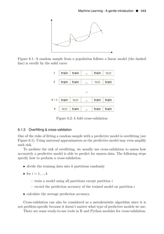
![164 • A Tour of Data Science: Learn R and Python in Parallel
But for pedagogical purposes, let’s do it step by step. We do the cross validation
using the Lasso regression we built in a previous chapter on the Boston dataset.
R
1 source(’../chapter5/lasso.R’)
2
3 library(caret)
4 library(MASS)
5 library(Metrics) # we use the rmse function from this package
6 k = 5
7
8 set.seed(42)
9 # if we set returnTrain = TRUE, we get the indices for train
partition
10 test_indices = createFolds(Boston$medv, k = k, list = TRUE,
returnTrain = FALSE)
11 scores = rep(NA, k)
12
13 for (i in 1:k){
14 lr = Lasso$new(200)
15 # we exclude the indices for test partition and train the
model
16 lr$fit(data.matrix(Boston[−test_indices[[i]], −ncol(Boston)]),
Boston$medv[−test_indices[[i]]], 100)
17 y_hat = lr$predict(data.matrix(Boston[test_indices[[i]], −ncol
(Boston)]))
18 scores[i] = rmse(Boston$medv[test_indices[[i]]], y_hat)
19 }
20 print(mean(scores))
Python
1 import sys
2 sys.path.append("..")
3
4 from sklearn.metrics import mean_squared_error
5 from sklearn.datasets import load_boston
6 from sklearn.model_selection import KFold
7 from chapter5.lasso import Lasso
8
9
10 boston = load_boston()
11 X, y = boston.data, boston.target
12](https://image.slidesharecdn.com/a-tour-of-data-science-learn-r-and-python-in-parallel-1st-edition-241027161058-87cda925/85/a-tour-of-data-science-learn-r-and-python-in-parallel-1st-edition-pdf-175-320.jpg)
![Machine Learning - A gentle introduction • 165
13 # create the partitions with k=5
14 k = 5
15 kf = KFold(n_splits=k)
16 # create a placeholder for the rmse on each test partition
17 scores = []
18
19 for train_index , test_index in kf.split(X):
20 X_train , X_test = X[train_index], X[test_index]
21 y_train , y_test = y[train_index], y[test_index]
22 # let’s train the model on the train partitions
23 lr = Lasso(200.0)
24 lr.fit(X_train , y_train , max_iter=100)
25 # now test on the test partition
26 y_hat = lr.predict(X_test)
27 # we calculate the root of mean squared error (rmse)
28 rmse = mean_squared_error(y_test , y_hat) ∗∗ 0.5
29 scores.append(rmse)
30
31 # average rmse from 5−fold cross−validation
32 print(sum(scores)/k)
Run the code snippets; we have the 5-fold cross-validation accuracy as follows.
R Python
1 chapter6 $r −f cv.R 1 chapter6 $python3.7 cv.py
2 [1] 4.978324 2 5.702339699398128
We add the line sys.path.append("..") in the Python code, otherwise it would
throw an error because of the import mechanism6
.
6.1.4 Evaluation metrics
In the example above, we measure the root of mean squared error (RMSE) as the
accuracy of the linear regression model. There are various metrics to evaluate the
accuracy of predictive models.
• Metrics for regression
For regression models, RMSE, mean absolute error (MAE)7
and mean absolute
percentage error (MAPE)8
are some of the commonly-used evaluation metrics.
You may have heard of the coefficient of determination ( 2
R or adjusted 2
R ) in
statistics. But from a predictive modelling perspective, 2
R is not a metric that
6
https://docs.python.org/3/reference/import.html
7
https://en.wikipedia.org/wiki/Mean_absolute_error
8
https://en.wikipedia.org/wiki/Mean_absolute_percentage_error](https://image.slidesharecdn.com/a-tour-of-data-science-learn-r-and-python-in-parallel-1st-edition-241027161058-87cda925/85/a-tour-of-data-science-learn-r-and-python-in-parallel-1st-edition-pdf-176-320.jpg)
![Machine Learning - A gentle introduction • 167
100% wrong, the resulting AUC is equal to 0. But if we know a binary-class
classification model always results in 100% wrong predictions, we can instead
use 1−ŷ as the corrected prediction and as a result we will get a perfect model
and the AUC based on the corrected prediction becomes 1. Actually, a model
using a completely random guess as the prediction leads to an AUC equal to
0.5. Thus, in practice the evaluated AUC is usually between 0.5 and 1.
There are also many other metrics, such as recalls, precisions, and F1 score10
.
The selection of evaluation metrics in predictive modelling is important but also
subjective. Sometimes we may also need to define a customized evaluation metric.
Many evaluation metrics can be found from the R package Metrics and the
Python module sklearn.metrics.
R Python
1 > set.seed(42) 1 >>> import numpy as np
2 > # regression metrics 2 >>> from sklearn.metrics
import mean_squared_error
3 > y = rnorm(n = 10,
, mean_absolute_error ,
mean = 10, sd = 2)
4 > y log_loss , roc_auc_score
5 [1] 12.741917 3
8.870604 >>> np.random.seed(42)
10.726257 11.265725 4 >>> # regression metrics
10.808537 9.787751 5 ...
6 [7] 13.023044 9.810682 6 >>> y = np.random.normal(10,
14.036847 9.874572 2, 10)
7 > # we use random numbers as 7 >>> y_hat = np.random.normal
the predictions (10.5, 2.2, 10)
8 > y_hat = rnorm(n = 10, 8 >>> mean_squared_error(y,
mean = 10.5, sd = 2.2)
y_hat) 0.5 #
9 > y_hat rmse
∗∗
10 [1] 13.370713 15.530620 9 3.0668667318485165
7.444506 9.886665 10 >>> mean_absolute_error(y,
10.206693 11.899091 y_hat) #
mae
11 [7] 9.874644 4.655798 11 2.1355703394788237
5.130973 13.404249 12 >>> # let’s define mape
12 > since it’s not available
13 > rmse(actual = y, predicted 13 ...
= y_hat) 14 >>> def mape(y, y_hat):
return np.mean(np.
14 [1] 4.364646 abs(y y_hat)/y_hat)
15 > mae(actual = y, predicted 15 ...
−
= y_hat) 16 >>> mape(y, y_hat)
16 [1] 3.540164 17 0.292059554974094
17 > mape(actual = y, predicted 18 >>> # classification metrics
= y_hat) 19 >>> y = np.random.binomial
18 [1] 0.3259014 (1, 0.25, 10)
10
https://en.wikipedia.org/wiki/Precision_and_recall](https://image.slidesharecdn.com/a-tour-of-data-science-learn-r-and-python-in-parallel-1st-edition-241027161058-87cda925/85/a-tour-of-data-science-learn-r-and-python-in-parallel-1st-edition-pdf-178-320.jpg)
![168 • A Tour of Data Science: Learn R and Python in Parallel
19 > # classification metrics 20 >>> y_hat = np.random.
20 > y = rbinom(n = 10, size = uniform(0, 1, 10)
1, prob=0.25) 21 >>> log_loss(y, y_hat)
21 > y 22 0.47071363776285635
22 [1] 0 0 0 1 0 1 1 0 1 0 23 >>> roc_auc_score(y, y_hat)
y_hat = runif(10, # auc
23 > 0, 1)
24 0.8095238095238095
24 > logLoss(y, y_hat)
25 [1] 0.4553994
26 > auc(y, y_hat)
27 [1] 0.8333333
6.1.5 Feature engineering & embedding
According to the explanation of feature engineering11
on wikipedia, feature engineer
ing is the process to use domain knowledge to create new features based on existing
features. In reality, it is not rare to see feature engineering leads to better prediction
accuracy. And sometimes I use feature engineering too. But I think feature engi
neering will be less and less useful in the future as the machine learning algorithms
become more and more intelligent.
Let’s consider three features x1, x2 and x3 and assume the actual model is spec
ified as y = f(x1, g(x2, x3)). After all, y is still a function of x1, x2 and x3, and
we can write it as y = h(x1, x2, x3). Thus, even without creating the new feature
x4 = g(x2, x3) explicitly, a universal approximator should be able to learn (i.e., ap
proximate) the function h from the data ideally. This idea is also supported by the
Kolmogorov–Arnold representation theorem12
which says any continuous real-valued
multivariate functions can be written as a finite composition of continuous functions
of a single variable.
2m m
) =
f(x1, ..., xm Φq
q=0 p
φq,p(xp) . (6.1)
=1
( )
As of today, since the machine learning algorithms are not that intelligent, it is
worth trying feature engineering especially when domain knowledge is available.
If you are familiar with dimension reduction, embedding can be considered as
something similar. Dimension reduction aims at reducing the dimension of X. It
sounds interesting and promising if we can transform the high-dimensional dataset
into a low-dimensional dataset and feed the dataset in a low dimension space to the
machine learning model. However, this may not be a good idea in general. For exam
ple, in supervised learning it is not guaranteed that the low-dimensional predictors
will keep all the information related to the response variable. Actually, many machine
learning models are capable of handling the high-dimensional predictors directly.
Embedding transforms the features into a new space, which usually has a lower
11
https://en.wikipedia.org/wiki/Feature_engineering
12
https://en.wikipedia.org/wiki/Kolmogorov-Arnold_representation_theorem](https://image.slidesharecdn.com/a-tour-of-data-science-learn-r-and-python-in-parallel-1st-edition-241027161058-87cda925/85/a-tour-of-data-science-learn-r-and-python-in-parallel-1st-edition-pdf-179-320.jpg)
![Machine Learning - A gentle introduction • 169
dimension. But generally embedding is not done by the traditional dimension re
duction techniques (for example, principal component analysis). In natural language
processing, a word can be embedded into a vector space by word2vec [12] (or other
techniques). When an instance is associated with an image, we may consider using
the penultimate layer’s output from a (deep) neural network-based image classifica
tion model to encode/embed the image into a space with lower dimension. It is also
popular to use embedding layers for embedding.
6.1.6 Collinearity
Collinearity is one of the cliches in machine learning. For non-linear models, collinear
ity is usually not a problem. For linear models, I recommend reading this discussion13
to see when it is not a problem.
6.1.7 Feature selection & parameter tuning
We have seen how the Lasso solutions of linear models can be used for feature se
lection in Chapter 6. What about non-linear models? There are some model-specific
techniques for feature selection. Also, there is a metaheuristic approach to select
features - cross-validation. Specifically, we can try different combinations of the fea
tures and use cross-validation to select the set of features which results in the best
cross-validation evaluation metric. However, the major problem of this approach is
its efficiency. When the number of features is too large, it is impossible to try all the
different combinations with limited computational resources. Thus, it is better to use
the model-specific feature selection techniques in practice.
To tune model parameters, such as the λ in Lasso, we can also use cross-validation.
But again, the efficiency is our major concern.
Can we have feature selection and parameter tuning done automatically? Actually,
automated machine learning14
has been a hot research topic in both academia and
industry. With the advance of machine learning theories, more intelligent algorithms
will be available which require less and less work on feature engineering and parameter
tuning (or neural network architecture searching).
6.2 GRADIENT BOOSTING MACHINE
In this section we will talk about one of the greatest supervised learning models
gradient boosting machine.
6.2.1 Decision tree
A decision tree consists of a bunch of nodes. In a decision tree there is a node with
no parent nodes, which is called root node. The node without any children is called
leaf node.
The length (number of nodes) of the longest path from the root node to a leaf
13
https://statisticalhorizons.com/multicollinearity
14
https://en.wikipedia.org/wiki/Automated_machine_learning](https://image.slidesharecdn.com/a-tour-of-data-science-learn-r-and-python-in-parallel-1st-edition-241027161058-87cda925/85/a-tour-of-data-science-learn-r-and-python-in-parallel-1st-edition-pdf-180-320.jpg)
![Machine Learning - A gentle introduction • 171
3 "Tree",
4 public = list(
5 left = NULL,
6 right = NULL,
7 variable_id = NULL,
8 break_point = NULL,
9 val = NULL,
10 initialize = function(left, right, variable_id , break_point ,
val) {
11 self$left = left
12 self$right = right
13 self$variable_id = variable_id
14 self$break_point = break_point
15 self$val = val
16 },
17 is_leaf = function() {
18 is.null(self$left) && is.null(self$right)
19 },
20 depth = function() {
21 if (self$is_leaf()) {
22 1
23 } else if (is.null(self$left)) {
24 1 + self$right$depth()
25 } else if (is.null(self$right)) {
26 1 + self$left$depth()
27 } else{
28 1 + max(self$left$depth(), self$right$depth())
29 }
30 },
31 predict_single = function(x) {
32 # if x is a vector
33 if (self$is_leaf()) {
34 self$val
35 } else{
36 if (x[self$variable_id] < self$break_point) {
37 self$left$predict_single(x)
38 } else{
39 self$right$predict_single(x)
40 }
41 }
42 },
43 predict = function(x) {
44 # if x is an array
45 preds = rep(0.0, nrow(x))
46 for (i in 1:nrow(x)) {](https://image.slidesharecdn.com/a-tour-of-data-science-learn-r-and-python-in-parallel-1st-edition-241027161058-87cda925/85/a-tour-of-data-science-learn-r-and-python-in-parallel-1st-edition-pdf-182-320.jpg)
![172 • A Tour of Data Science: Learn R and Python in Parallel
47 preds[i] = self$predict_single(x[i, ])
48 }
49 preds
50 },
51 print = function() {
52 # we can call print(tree), similar to the special method
in Python
53 cat("variable_id:", self$variable_id , "n")
54 cat("break at:", self$break_point , "n")
55 cat("is_leaf:", self$is_leaf(), "n")
56 cat("val:", self$val, "n")
57 cat("depth:", self$depth(), "n")
58 invisible(self)
59 }
60 )
61 )
Python chapter6/tree.py
1 class Tree:
2 def __init__(self, left, right, variable_id , break_point ,
val):
3 self.left = left
4 self.right = right
5 self.variable_id = variable_id
6 self.break_point = break_point
7 self.val = val
8
9 @property
10 def is_leaf(self):
11 return self.left is None and self.right is None
12
13 def _predict_single(self, x):
14 if self.is_leaf:
15 return self.val
16 if x[self.variable_id] < self.break_point:
17 return self.left._predict_single(x)
18 else:
19 return self.right._predict_single(x)
20
21 def predict(self, x):
22 return [self._predict_single(e) for e in x]
23
24 @property](https://image.slidesharecdn.com/a-tour-of-data-science-learn-r-and-python-in-parallel-1st-edition-241027161058-87cda925/85/a-tour-of-data-science-learn-r-and-python-in-parallel-1st-edition-pdf-183-320.jpg)
![174 • A Tour of Data Science: Learn R and Python in Parallel
4 > node_4 = Tree$new(NULL, 3 >>> node_3 = Tree(None, None
NULL, NULL, NULL, 4.5) , None, None, 2.4)
5 > node_1 = Tree$new(node_3 ,
4 >>> node_4 = Tree(None, None
node_4 , 1, 10.5,
, None, None, 4.5)
NULL)
> node_0 = Tree$new(node_1 , 5
6 >>> node_1 = Tree(node_3,
node_2 , 2, node_4, )
3. 0, 10.5,
2, None
NULL) 6 >>> node_0 = Tree(node_1,
7 > print(node_0) node_2, 1, 3.2, None)
8 variable_id: 2 7 >>>
9 break at: 3.2 8 >>> print(node_0)
10 is_leaf: FALSE 9 variable_id: 1
11 val: 10 break_at: 3.2
12 depth: 3 11 val: None
13 > print(node_4) 12 is_leaf: False
14 variable_id: 13 depth: 3
15 break at: 14 >>> print(node_4)
16 is_leaf: TRUE 15 variable_id: None
17 val: 4.5 16 break_at: None
18 depth: 1 17 val: 4.5
19 > x = array(c(10, 0.5), 18 is_leaf: True
c(1, 2))
19
20 > node_0$predict(x)
depth: 1
20 >>> x = [[10, 0.5]]
21 [1] 2.4
21 >>> node_0.predict(x)
22 [2.4]
It’s worth noting decision trees can approximate universally.
6.2.2 Tree growing in gradient boosting machine
What is a gradient boosting machine (GBM) (or gradient boosting regression)? Es
sentially, a GBM is just a forest of decision trees. If you have heard of random forest
(RF), you may know that a random forest is also a bunch of trees. What is the
difference between a GBM and RF?
Looking at the fitted trees from RF and GBM, there is no way to tell if the trees
are fitted by an RF or a GBM. The major difference is how these trees are trained,
rather than the trees themselves. A minor difference is how these trees are used for
prediction. In many RF implementations, the prediction for an instance is the average
prediction of each tree within the forest. If it is a classification task, there are two
ways to get the final prediction — (a) predict the class with majority voting directly,
i.e., the predicted class is the one with highest frequency among the predicted classes
of all trees; (b) predict the probability based on the frequencies, for example, if among
five trees there are three trees output class 1 then the predicted probability of class 1
is equal to 3/5. In many GBM implementations, the prediction (for regression tasks)
is the sum of the predictions of individual trees.
GBM fits trees sequentially, but RF fits trees independently. The obvious advan](https://image.slidesharecdn.com/a-tour-of-data-science-learn-r-and-python-in-parallel-1st-edition-241027161058-87cda925/85/a-tour-of-data-science-learn-r-and-python-in-parallel-1st-edition-pdf-185-320.jpg)
![176 • A Tour of Data Science: Learn R and Python in Parallel
n t 1
L(t)
−
= ( i) − ft( 2
yi − fl(x xi)) (6.4)
i=1 l=1
In practice, a regularized loss function (6.5) is used instead of (6.3) to reduce
overfitting.
n t 1
L(t)
−
= (yi − fl(xi) − ft(xi))2
+ Φ(ft). (6.5)
i=1 l=1
Let’s follow the paper [6] and use the number of leaves as well as the L2 penalty
of the values (also called weights) of the leaves for regularization. The loss function
then becomes
n t 1 T
L(t)
−
1
i
= (yi
=1
− fl(xi)
l=1
− 2
f ( 2
t xi)) + γT + λ ωj , (6.6)
2 j=1
where ωj is the value associated with the jth leaf of the current tree.
Again, we get an optimization problem, i.e., to minimize the loss function (6.6).
The minimization problem can also be viewed as a quadratic programming problem.
However, it seems different from the other optimization problems we have seen before,
in the sense that the decision tree ft is a non-parametric model. A model is non-
parametric if the model structure is learned from the data rather than pre-determined.
A common approach used in GBM is the second-order approximation. By second-
order approximation, the loss function becomes
n t 1 n T
L(t)
−
1 1
≈ (yi − fl(xi))2
+ ( (x ) + 2
gift i
2
hift(xi)2
) + γT +
2
λ ωj , (6.7)
i=1 l=1 i=1 j=1
where t−1
gi = 2(ft(xi)+ l=1 fl(xi)−yi) and hi = 2 are the first- and the second-order
derivatives of the function ( t−1
yi − l=1 fl(xi) − ft(xi))2
with respect to the function
ft(xi).
Let’s implement the function to calculate g and h and put them into util.py.
Python chapter6/util.py
1 import numpy as np
2
3 def gh_lm(actual , pred):
4 ’’’
5 gradient and hessian for linear regression loss
6 ’’’
7 return 2∗(pred−actual), 2.0
Since the first item is a constant, let’s ignore it.](https://image.slidesharecdn.com/a-tour-of-data-science-learn-r-and-python-in-parallel-1st-edition-241027161058-87cda925/85/a-tour-of-data-science-learn-r-and-python-in-parallel-1st-edition-pdf-187-320.jpg)
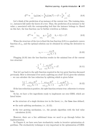
![178 • A Tour of Data Science: Learn R and Python in Parallel
More specifically, we apply the stochasticity both instance-wise and feature-wise.
Instance-wise, when we fit a new tree, we randomly get a subsample from the train
ing sample. And feature-wise, we randomly select a few features/variables when we fit
a new tree. The stochasticity technique could help to reduce overfitting. The extent
of the stochasticity can be controlled by arguments.
Like the gradient decent algorithm, in GBM there is also a learning rate parameter
which scales the values of the leaves after a tree is fitted.
In practice, we may also not want to have too few instances under a leaf, to reduce
potential overfitting. When there are two few instances under a leaf, we may just stop
the splitting process.
Now we have almost all the ingredients to make a working GBM. Let’s define the
split_node function in the code snippet below.
Python chapter6/grow.py
1 from tree import Tree
2 import numpy as np
3 import pdb
4
5
6 def split_node(f_in_tree , x_in_node , x_val_sorted ,
x_index_sorted , g_tilde , h_tilde , lam, gamma, min_instances)
:
7 ’’’
8 f_in_tree: a list of booleans indicating which variable/
feature is selected in the tree
9 x_in_ndoe: a list of booleans indicating which instance is
used in the tree
10 x_val_sorted: a nested list, x_val_sorted[feature index] is
a list of instance values
11 x_index_sorted: a nested list, x_index_sorted[feature index]
is a list of instance indexes
12 g_tilde: first order derivative
13 h_tilde: second order derivative
14 lam: lambda for regularization
15 gamma: gamma for regularization
16 min_instances: the minimal number of instances under a leaf
17 at the beginning we assume all instances are on the right
18 ’’’
19 if sum(x_in_node) < min_instances:
20 return False, None, None, None, None, None, None
21 best_break = 0.0
22 best_feature , best_location = 0, 0
23 ncol, nrow = len(f_in_tree), len(x_in_node)
24 g, h = 0.0, 0.0](https://image.slidesharecdn.com/a-tour-of-data-science-learn-r-and-python-in-parallel-1st-edition-241027161058-87cda925/85/a-tour-of-data-science-learn-r-and-python-in-parallel-1st-edition-pdf-189-320.jpg)
![Machine Learning - A gentle introduction • 179
25 for i, e in enumerate(x_in_node):
26 if e:
27 g += g_tilde[i]
28 h += h_tilde[i]
29 base_score = g∗g/(h+lam)
30 score_reduction = np.inf
31
−
best_w_left , best_w_right = None, None
32 for k in range(ncol):
33 if f_in_tree[k]:
34 # if the feature is selected for this tree
35 best_n_left_k = 0
36 n_left_k = 0
37 # feature is in the current tree
38 g_left , h_left = 0.0, 0.0
39 g_right , h_right = g−g_left , h−h_left
40 # score reduction for current feature k
41 score_reduction_k = −np.inf
42 for i in range(nrow):
43 # for each in sample , we try to split on it
44 index = x_index_sorted[k][i]
45 if x_in_node[index]:
46 n_left_k += 1
47 best_n_left_k += 1
48 g_left += g_tilde[index]
49 g_right = g−g_left
50 h_left += h_tilde[index]
51 h_right = h−h_left
52 # new score reduction
53 score_reduction_k_i = g_left∗g_left/(h_left+
lam) +
54 (g_right∗g_right)/(h_right+lam)−
base_score
55 if score_reduction_k <= score_reduction_k_i:
56 best_n_left_k = n_left_k
57 best_break_k = x_val_sorted[k][i]
58 best_location_k = i
59 score_reduction_k = score_reduction_k_i
60 w_left_k = −g_left/(h_left+lam)
61 w_right_k = −g_right/(h_right+lam)
62
63 # if the score reduction on feature k is a better
candidate
64 if score_reduction_k >= score_reduction:
65 score_reduction = score_reduction_k
66 best_feature = k](https://image.slidesharecdn.com/a-tour-of-data-science-learn-r-and-python-in-parallel-1st-edition-241027161058-87cda925/85/a-tour-of-data-science-learn-r-and-python-in-parallel-1st-edition-pdf-190-320.jpg)
![180 • A Tour of Data Science: Learn R and Python in Parallel
67 best_break = best_break_k
68 best_location = best_location_k
69 best_w_left = w_left_k
70 best_w_right = w_right_k
71 return 0.5∗score_reduction >= gamma, best_feature ,
best_break , best_location , best_w_left , best_w_right ,
score_reduction
72
73
74 def grow_tree(current_tree , f_in_tree , x_in_node , max_depth ,
x_val_sorted , x_index_sorted , y, g_tilde , h_tilde , eta, lam,
gamma, min_instances):
75 ’’’
76 current_tree: the current tree to grow, i.e., a node
77 f_in_tree , x_in_node , x_val_sorted , x_index_sorted: see
split_node function
78 max_depth: maximinum depth to grow
79 eta: learning rate
80 y: the response variable
81 ’’’
82 nrow = len(y)
83 if max_depth == 0:
84 return
85 # check if we need a split
86 do_split , best_feature , best_break , best_location , w_left ,
w_right , _ = split_node(
87 f_in_tree , x_in_node , x_val_sorted , x_index_sorted ,
g_tilde , h_tilde , lam, gamma, min_instances)
88
89 if do_split:
90 # update the value/weight with the learning rate eta
91 w_left_scaled = w_left∗eta
92 w_right_scaled = w_right∗eta
93 current_tree.variable_id = best_feature
94 current_tree.break_point = best_break
95 current_tree.val = None
96
97 # initialize the left subtree
98 current_tree.left = Tree(None, None, None, None,
w_left_scaled)
99 # initialize the right subtree
100 current_tree.right = Tree(None, None, None, None,
w_right_scaled)
101 # update if an instance is in left or right
102 x_in_left_node = [False]∗len(x_in_node)](https://image.slidesharecdn.com/a-tour-of-data-science-learn-r-and-python-in-parallel-1st-edition-241027161058-87cda925/85/a-tour-of-data-science-learn-r-and-python-in-parallel-1st-edition-pdf-191-320.jpg)
![Machine Learning - A gentle introduction • 181
103 x_in_right_node = [False]∗len(x_in_node)
104 for i in range(nrow):
105 index = x_index_sorted[best_feature][i]
106 if x_in_node[index]:
107 if i <= best_location:
108 x_in_left_node[index] = True
109 else:
110 x_in_right_node[index] = True
111 # recursively grow its left subtree
112 grow_tree(current_tree.left, f_in_tree , x_in_left_node ,
max_depth−1,
113 x_val_sorted , x_index_sorted , y, g_tilde ,
h_tilde , eta, lam, gamma, min_instances)
114 # recursively grow its right subtree
115 grow_tree(current_tree.right, f_in_tree , x_in_right_node
, max_depth−1,
116 x_val_sorted , x_index_sorted , y, g_tilde ,
h_tilde , eta, lam, gamma, min_instances)
117 else:
118 # current node is a leaf, so we update the value/weight
of the leaf
119 g, h = 0.0, 0.0
120 for i, e in enumerate(x_in_node):
121 if e:
122 g += g_tilde[i]
123 h += h_tilde[i]
124 w_left_scaled = −g/(h+lam)∗eta
125 current_tree.val = w_left_scaled
And the implementation of the GBM class is given below.
Python chapter6/gbm.py
1 from tree import Tree
2 from grow import grow_tree , split_node
3 from utils import gh_lm, rmse
4 import numpy as np
5
6
7 class GBM:
8 def __init__(self, x_train , y_train , depth, eta, lam, gamma,
sub_sample , sub_feature , min_instances=2):
9 ’’’
10 x_train , y_train: training data
11 depth: maximum depth of each tree](https://image.slidesharecdn.com/a-tour-of-data-science-learn-r-and-python-in-parallel-1st-edition-241027161058-87cda925/85/a-tour-of-data-science-learn-r-and-python-in-parallel-1st-edition-pdf-192-320.jpg)
![182 • A Tour of Data Science: Learn R and Python in Parallel
12 eta: learning rate
13 lam and gamma: regularization parameters
14 sub_sample: control the instance−wise stochasticity
15 sub_feature: control the feature−wise stochasticity
16 min_instances: control the mimimum number of instances
under a leaf
17 ’’’
18 self.n = len(x_train)
19 self.m = len(x_train[0])
20 self.x_train = x_train
21 self.y_train = y_train
22 self.x_test , self.y_test = None, None
23 self.depth = depth
24 self.eta = eta
25 self.lam = lam
26 self.gamma = gamma
27 self.sub_sample = sub_sample
28 self.sub_feature = sub_feature
29 self.min_instances = min_instances
30
31 self.y_tilde = [0]∗len(y_train)
32 self.g_tilde , self.h_tilde = [0] ∗
33 len(self.y_tilde), [0] len(self.y_tilde)
34
∗
for i in range(len(self.y_tilde)):
35 self.g_tilde[i], self.h_tilde[i] = gh_lm(
36 y_train[i], self.y_tilde[i])
37 x_columns = x_train.transpose()
38 self.nf = min(self.m, max(1, int(sub_feature∗self.m)))
39 self.x_val_sorted = np.sort(x_columns)
40 self.x_index_sorted = np.argsort(x_columns)
41 self.forest = []
42
43 def set_test_data(self, x_test , y_test):
44 self.x_test = x_test
45 self.y_test = y_test
46
47 def predict(self, x_new):
48 y_hat = np.array([0.0]∗len(x_new))
49 for tree in self.forest:
50 y_hat += np.array(tree.predict(x_new))
51 return y_hat
52
53 def fit(self, max_tree , seed=42):
54 np.random.seed(seed)
55 self.forest = []](https://image.slidesharecdn.com/a-tour-of-data-science-learn-r-and-python-in-parallel-1st-edition-241027161058-87cda925/85/a-tour-of-data-science-learn-r-and-python-in-parallel-1st-edition-pdf-193-320.jpg)
![Machine Learning - A gentle introduction • 183
56 i = 0
57 while i < max_tree:
58 # let’s fit tree i
59 # instance−wise stochasticity
60 x_in_node = np.random.choice([True, False], self.n,
p=[
61 self.sub_sample , 1−self
.sub_sample])
62 # feature−wise stochasticity
63 f_in_tree_ = np.random.choice(
64 range(self.m), self.nf, replace=False)
65 f_in_tree = np.array([False]∗self.m)
66 for e in f_in_tree_:
67 f_in_tree[e] = True
68 del f_in_tree_
69 # initialize the root of this tree
70 root = Tree(None, None, None, None, None)
71 # grow the tree from root
72 grow_tree(root, f_in_tree , x_in_node , self.depth−1,
self.x_val_sorted ,
73 self.x_index_sorted , self.y_train , self.
g_tilde , self.h_tilde , self.eta, self.
lam, self.gamma, self.min_instances)
74 if root is not None:
75 i += 1
76 self.forest.append(root)
77 else:
78 next
79 for j in range(self.n):
80 self.y_tilde[j] += self.forest[−1].
_predict_single(
81 self.x_train[j])
82 self.g_tilde[j], self.h_tilde[j] = gh_lm(
83 self.y_train[j], self.y_tilde[j])
84 if self.x_test is not None:
85 # test on the testing instances
86 y_hat = self.predict(self.x_test)
87 print("iter: {0:>4} rmse: {1:1.6f}".format(
88 i, rmse(self.y_test , y_hat)))
Now let’s see the performance of our GBM implemented from scratch.
Python chapter6/test_gbm.py
1 from gbm import GBM](https://image.slidesharecdn.com/a-tour-of-data-science-learn-r-and-python-in-parallel-1st-edition-241027161058-87cda925/85/a-tour-of-data-science-learn-r-and-python-in-parallel-1st-edition-pdf-194-320.jpg)
![184 • A Tour of Data Science: Learn R and Python in Parallel
2 import numpy as np
3 from sklearn import datasets
4 from sklearn.utils import shuffle
5
6
7 def get_boston_data(seed=42):
8 boston = datasets.load_boston()
9 X, y = shuffle(boston.data, boston.target , random_state=seed
)
10 X = X.astype(np.float32)
11 offset = int(X.shape[0] ∗ 0.8)
12 X_train , y_train = X[:offset], y[:offset]
13 X_test , y_test = X[offset:], y[offset:]
14 return X_train , y_train , X_test, y_test
15
16 if __name__ == "__main__":
17 X_train , y_train , X_test, y_test = get_boston_data(42)
18 gbm = GBM(X_train , y_train , depth=6, eta=0.05, lam=1.0,
19 gamma=1, sub_sample=0.5, sub_feature=0.7)
20 gbm.set_test_data(X_test , y_test)
21 gbm.fit(max_tree=200)
Running the code above, we have output as below.
Python
1 chapter6 $python3.7 test_gbm.py
2 iter: 1 rmse: 23.063019
3 iter: 2 rmse: 21.997972
4 iter: 3 rmse: 21.026602
5 iter: 4 rmse: 20.043397
6 iter: 5 rmse: 19.210746
7 ...
8 iter: 196 rmse: 2.560747
9 iter: 197 rmse: 2.544847
10 iter: 198 rmse: 2.541102
11 iter: 199 rmse: 2.537366
12 iter: 200 rmse: 2.535143
We don’t implement the model in R, but it is not difficult to do based on the
Python implementation above.
GBM can be used with various loss functions, and the major difference is the
implementation of the first-/second-order derivatives, i.e., g and h.
Regardless of the performance, there are two major missing features in our im
plementation: a) cross-validation and b) early stopping. We have talked about cross](https://image.slidesharecdn.com/a-tour-of-data-science-learn-r-and-python-in-parallel-1st-edition-241027161058-87cda925/85/a-tour-of-data-science-learn-r-and-python-in-parallel-1st-edition-pdf-195-320.jpg)
![Machine Learning - A gentle introduction • 185
validation, but what is early stopping? It is a very useful technique in GBM. Usually,
the cross-validated loss decreases when we add new trees at the beginning and at
a certain point, the loss may increase when more trees are fitted (due to overfit
ting). Thus, we may select the best number of trees based on the cross-validated loss.
Specifically, stop the fitting process when the cross-validated loss doesn’t decrease.
In practice, we don’t want to stop the fitting immediately when the cross-validated
loss starts increasing. Instead, we specify a number of trees, e.g., 50, as a buffer, after
which the fitting process should stop if cross-validated loss doesn’t decrease.
Early stopping is also used in other machine learning models, for example, neural
network. Ideally, we would like to have early stopping based on the cross-validated
loss. But when the training process is time-consuming, it’s fine to use the loss on a
testing dateset16
.
The commonly used GBM packages include XGBoost17
, LightGBM18
and CatBoost
19
. Let’s see how to use XGBoost for the same regression task on the Boston dataset.
R chapter6/xgb.R
1 library(xgboost)
2 library(MASS)
3 library(Metrics)
4 set.seed(42)
5 train_index = sample(nrow(Boston), floor(0.8 ∗ nrow(Boston)),
replace = FALSE)
6 Boston = data.matrix(Boston)
7 target_col = which(colnames(Boston) == ’medv’)
8 X_train = Boston[train_index , −target_col]
9 y_train = Boston[train_index , target_col]
10 X_test = Boston[−train_index , −target_col]
11 y_test = Boston[−train_index , target_col]
12 # prepare the data for training and testing
13 dTrain = xgb.DMatrix(X_train , label = y_train)
14 dTest = xgb.DMatrix(X_test)
15 params = list(
16 "booster" = "gbtree",
17 "objective" = "reg:linear",
18 "eta" = 0.1,
19 "max_depth" = 5,
20 "subsample" = 0.6,
21 "colsample_bytree" = 0.8,
22 "min_child_weight" = 2
23 )
16
https://en.wikipedia.org/wiki/Early_stopping
17
https://github.com/dmlc/xgboost
18
https://github.com/microsoft/LightGBM
19
https://github.com/catboost/catboost](https://image.slidesharecdn.com/a-tour-of-data-science-learn-r-and-python-in-parallel-1st-edition-241027161058-87cda925/85/a-tour-of-data-science-learn-r-and-python-in-parallel-1st-edition-pdf-196-320.jpg)
![186 • A Tour of Data Science: Learn R and Python in Parallel
24 # run the cross−validation
25 hist = xgb.cv(
26 params = params,
27 data = dTrain ,
28 nrounds = 500,
29 early_stopping_rounds = 50,
30 metrics = ’rmse’,
31 nfold = 5,
32 verbose = FALSE
33 )
34 # since we have the best number of trees from cv, let’s train
the model with this number of trees
35 model = xgb.train(params , nrounds = hist$best_iteration , data =
dTrain)
36 pred = predict(model, dTest)
37
38 cat(
39 "rmse on testing instances is",
40 rmse(y_test, pred),
41 "with",
42 hist$best_iteration ,
43 "trees"
44 )
Python chapter6/xgb.py
1 import xgboost as xgb
2 from sklearn import datasets
3 from sklearn.utils import shuffle
4 from sklearn.metrics import mean_squared_error
5 import numpy as np
6
7 seed = 42
8 boston = datasets.load_boston()
9 X, y = shuffle(boston.data, boston.target , random_state=seed)
10 X = X.astype(np.float32)
11 offset = int(X.shape[0] ∗ 0.8)
12 X_train , y_train = X[:offset], y[:offset]
13 X_test , y_test = X[offset:], y[offset:]
14
15 params = {’booster’: ’gbtree’, ’objective’: ’reg:linear’, ’
learning_rate’: 0.1,
16 ’max_depth’: 5, ’subsample’: 0.6, ’colsample_bytree’:
0.8, ’min_child_weight’: 2}](https://image.slidesharecdn.com/a-tour-of-data-science-learn-r-and-python-in-parallel-1st-edition-241027161058-87cda925/85/a-tour-of-data-science-learn-r-and-python-in-parallel-1st-edition-pdf-197-320.jpg)
![Machine Learning - A gentle introduction • 187
17
18 # prepare the data for training and testing
19 dtrain = xgb.DMatrix(data=X_train , label=y_train , missing=None)
20 dtest = xgb.DMatrix(X_test)
21
22 # run 5−fold cross−validation with maximum 1000 trees, and try
to minimize the metric rmse
23 # early stopping 50 trees
24 hist = xgb.cv(params , dtrain=dtrain , nfold=5,
25 metrics=[’rmse’], num_boost_round=1000, maximize=
False, early_stopping_rounds=50)
26
27 # find the best number of trees from the cross−validation
history
28 best_number_trees = hist[’test−rmse−mean’].idxmin()
29
30 # since we have the best number of trees from cv, let’s train
the model with this number of trees
31 model = xgb.train(params , dtrain , num_boost_round=
best_number_trees)
32 pred = model.predict(dtest)
33 print(
34 f"rmse on testing instances is {mean_squared_error(pred,
y_test)∗∗0.5:.6f} with {best_number_trees} trees")
The parameters subsample and colsample_bytree control the stochasticity, within
the range of [0, 1]. If we set these two parameters to 1, then all instances and all
features are selected for fitting every tree.
The two code snippets illustrate a minimal workflow of fitting a GBM model.
First, we conduct (hyper) parameter tuning (such as learning rate, number of trees,
regularization parameters, stochasticity parameters) with cross-validation, and next
we train the model with the tuned parameters.
Running the code snippets, we have the following results.
R Python
1 > source(’xgb.R’) 1 chapter6 $python3.7 xgb.py
2 rmse on testing instances 2 rmse on testing instances is
is 2.632298 with 83 trees 2.736038 with 179 trees
In XGBoost, we could also use linear regression models as the booster (or base
learner) instead of decision trees. However, when ’booster’:’gblinear’ is used, the
sum of the prediction from all boosters in the model is equivalent to the prediction](https://image.slidesharecdn.com/a-tour-of-data-science-learn-r-and-python-in-parallel-1st-edition-241027161058-87cda925/85/a-tour-of-data-science-learn-r-and-python-in-parallel-1st-edition-pdf-198-320.jpg)
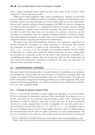
![�
Machine Learning - A gentle introduction • 189
Figure 6.4: Original vs. transformed data points via PCA
1
coordinate have the largest variance, and w1xi is called the first principal component.
And we can find the remaining transformations and principal components iteratively.
So now we see how the PCA is formulated as an optimization problem. However,
under the above setting, there are infinite solutions for wk. We usually add a con
straint on wk in PCA, i.e., |wk| = 1. The solution to this optimization problem is
surprisingly elegant - the optimal wk is the eigenvectors of the covariance matrix of
x. Now let’s try to conduct a PCA with eigen decomposition (it can also be done
with other decompositions).
R
1 > set.seed(42)
2 > n = 1000
3 > # we simulate some data points on a 2d plane
4 > x1 = rexp(n)
5 > x2 = x1∗3 + rnorm(n, 12, 2)
6 > x = cbind(x1, x2)
7 > # total marginal variance
8 > sum(diag(cov(x)))
9 [1] 15.54203
10 > pca_vectors = eigen(cov(x))$vectors
11 > # find the projection on the new coordinate system
12 > z = x %∗% pca_vectors
13 > # total marginal variance after transformation
14 > sum(diag(cov(z)))
15 [1] 15.54203
In fact, it does not matter if the raw data points are centered or not if the eigen
decomposition is on the covariance matrix. If you prefer to decompose x x directly,](https://image.slidesharecdn.com/a-tour-of-data-science-learn-r-and-python-in-parallel-1st-edition-241027161058-87cda925/85/a-tour-of-data-science-learn-r-and-python-in-parallel-1st-edition-pdf-200-320.jpg)
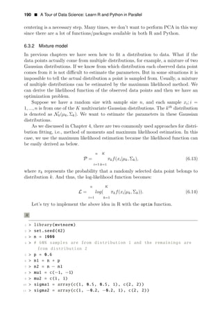
![Machine Learning - A gentle introduction • 191
12 > x1 = rmvnorm(n = n1, mean = mu1, sigma = sigma1)
13 > x2 = rmvnorm(n = n2, mean = mu2, sigma = sigma2)
14 > x = rbind(x1, x2)
15 > # let’s permute x
16 > x_permuted = x[sample(n), ]
17 >
18 >
19 > log_lik = function(theta, x) {
20 + # theta is a vector of length 9
21 + # first let’s reparametrize the parameters
22 + mu1 = theta[1:2]
23 + mu2 = theta[3:4]
24 + sigma1 = array(c(theta[5], theta[6], theta[6], theta[5]), c
(2, 2))
25 + sigma2 = array(c(theta[7], theta[8], theta[8], theta[7]), c
(2, 2))
26 + pi_1 = theta[9]
27 + pi_2 = 1 − pi_1
28 + # we return the negative log−likelihood
29 + − sum(log(pi_1 ∗ dmvnorm(x, mu1, sigma1) + pi_2 ∗ dmvnorm(x,
mu2, sigma2)))
30 + }
31 >
32 > gaussian_mixture_mle = function(x) {
33 + # par as the initial values
34 + optim(
35 + par = c(0, 0, 0, 0, 1, 0, 1, 0, 0.5),
36 + fn = log_lik ,
37 + x = x,
38 + method = "L−BFGS−B",
39 + control = list(trace = 1, maxit = 1000)
40 + )$par
41 + }
42 > res = gaussian_mixture_mle(x_permuted)
43 iter 10 value 3299.463920
44 final value 3299.463917
45 converged
46 > mu1_hat = res[1:2]
47 > mu2_hat = res[3:4]
48 > sigma1_hat = array(c(res[5], res[6], res[6], res[5]), c(2, 2))
49 > sigma2_hat = array(c(res[7], res[8], res[8], res[7]), c(2, 2))
50 > pi = res[9]
51 > print(mu1_hat)
52 [1] −0.2221727 −0.2171368
53 > print(mu2_hat)](https://image.slidesharecdn.com/a-tour-of-data-science-learn-r-and-python-in-parallel-1st-edition-241027161058-87cda925/85/a-tour-of-data-science-learn-r-and-python-in-parallel-1st-edition-pdf-202-320.jpg)
![192 • A Tour of Data Science: Learn R and Python in Parallel
54 [1] −0.2221727 −0.2171368
55 > print(sigma1_hat)
56 [,1] [,2]
57 [1,] 1.986965 1.196158
58 [2,] 1.196158 1.986965
59 > print(sigma2_hat)
60 [,1] [,2]
61 [1,] 1.986965 1.196158
62 [2,] 1.196158 1.986965
63 > print(pi)
64 [1] 0.5
The estimates of parameters are not satisfactory, why? Remember we have empha
sized the importance of convexity in Chapter 6. Actually, the log-likelihood function
given in (6.14) is not convex. For non-convex problems, the optim function may not
converge. In practice, EM algorithm22
is frequently applied for mixture model.
The theory of EM algorithm is out of the scope of this book. Let’s have a look
at the implementation for this specific problem. Basically, there are two steps, i.e.,
E-step and M-step which run in an iterative fashion. In the tth
E-step, we update
the membership probability wi,k that represents the probability that xi belongs to
distribution k, based on the current parameter estimates as follows.
(t)
(
(t)
Σ
(t)
(t) αk f xi|μk , k )
wi,k = .
K (t)
(
(
Σ
(
|
t) t)
(6.15)
k=1 αk f xi μk , k )
And in the tth
M-step, for each k we update the parameters as follows.
n (t)
(t+1)
=
i=1 wi,k
αk
n
(t+1)
μk =
n (t)
i=1 wi,kxi
(6.16)
n (t)
i=1 wi,k
(t+1)
n (t) (t) (t)
i=1 wi,k(xi − μk )(xi − μk )1
Σk =
The Python code below implements the
n (t)
i=1 wi,k
above EM update schedule for a Gaussian
mixture model.
Python chapter6/gmm.py
1 import numpy as np
2
3 class GaussianMixture:
22
https://en.wikipedia.org/wiki/Expectation-maximization_algorithm](https://image.slidesharecdn.com/a-tour-of-data-science-learn-r-and-python-in-parallel-1st-edition-241027161058-87cda925/85/a-tour-of-data-science-learn-r-and-python-in-parallel-1st-edition-pdf-203-320.jpg)
![Machine Learning - A gentle introduction • 193
4 """
5 X − n∗m array
6 K − the number of distributions/clusters
7 seed − random seed for reproducibility
8 """
9
10 def __init__(self, X, K):
11 self.X = X
12 self.K = K
13 self.n, self.p = X.shape
14 self.mu_list = [np.random.uniform(−1, 1, self.p)
15 for _ in range(self.K)]
16 self.sigma_list = [np.diag([1.0]∗self.p) for _ in range(
self.K)]
17 self.alphas = np.ones(self.K)/self.K
18
19 def E_step(self):
20 # first, we update the membership weight for each data
point, i.e., which distribution x_i belongs to
21 # we compute the pdf for each data point and each
distribution , stored in w(i,j)
22 pdf_list = np.zeros((self.n, self.K))
23 c = (2∗np.pi)∗∗(self.p/2)
24 for i in range(self.K):
25 x_centered = self.X − self.mu_list[i]
26 sigma_inversed = np.linalg.inv(self.sigma_list[i])
27 sigma_det = np.sqrt(np.linalg.det(self.sigma_list[i
]))
28 for j in range(self.n):
29 pdf_list[j, i] = 1.0/(c∗sigma_det)∗
30 np.exp(−0.5 ∗ x_centered[j, :][None, :] @
sigma_inversed @ x_centered[j, :][:,
None])
31 # we calculate the posterior probability
32 posterior_prob = pdf_list∗self.alphas
33 # now let’s update the memembership probability
34 w = posterior_prob/np.sum(posterior_prob , axis=1)[:,
None]
35 return w
36
37 def M_step(self, w):
38 # we update the mu and sigma based on the updated weight
from the E step
39 for i in range(self.K):
40 self.alphas[i] = np.mean(w[:, i])](https://image.slidesharecdn.com/a-tour-of-data-science-learn-r-and-python-in-parallel-1st-edition-241027161058-87cda925/85/a-tour-of-data-science-learn-r-and-python-in-parallel-1st-edition-pdf-204-320.jpg)
![194 • A Tour of Data Science: Learn R and Python in Parallel
41 self.mu_list[i] = np.sum(
42 self.X∗w[:, i][:, None], axis=0)/np.sum(w[:, i])
43 x_centered = self.X − self.mu_list[i]
44 self.sigma_list[i] = x_centered.transpose() @ (
45 x_centered∗w[:, i][:, None])/np.sum(w[:, i])
46
47 def fit(self, maxit=100, verbose=False):
48 for _ in range(maxit):
49 w = self.E_step()
50 self.M_step(w)
51 if verbose:
52 print("mu: {}".format(self.mu_list))
53 print("sigma: {}".format(self.sigma_list))
54
55 def __repr__(self):
56 return "mu: {}n, sigma: {}n, alpha: {}n".format(self.
mu_list , self.sigma_list , self.alphas)
For space-saving, we use a third-party package in R rather than implementing
from scratch.
R
1 > library(mixtools)
2 > fit = mvnormalmixEM(x_permuted , maxit = 1000, k = 2)
3 number of iterations= 278
4 > summary(fit)
5 summary of mvnormalmixEM object:
6 comp 1 comp 2
7 lambda 0.669674 0.330326
8 mu1 −0.893166 −0.859121
9 mu2 1.137988 1.084453
10 loglik at estimate: −3211.291
11 > print(fit$sigma)
12 [[1]]
13 [,1] [,2]
14 [1,] 1.1086853 0.6670415
15 [2,] 0.6670415 1.2275707
16
17 [[2]]
18 [,1] [,2]
19 [1,] 0.9821523 −0.3748227
20 [2,] −0.3748227 1.0194300
21
22 # let’s also infer the distribution for each data point](https://image.slidesharecdn.com/a-tour-of-data-science-learn-r-and-python-in-parallel-1st-edition-241027161058-87cda925/85/a-tour-of-data-science-learn-r-and-python-in-parallel-1st-edition-pdf-205-320.jpg)
![Machine Learning - A gentle introduction • 195
Figure 6.5: Data points clustered by a Gaussian mixture model
23 z = as.integer(
24 fit$lambda[1] ∗ dmvnorm(x_permuted , fit$mu[[1]], fit$sigma
[[1]]) > fit$lambda[2] ∗
25 dmvnorm(x_permuted , fit$mu[[2]], fit$sigma[[2]])
26 ) + 1
In the above code, zi represents the membership probability. We plot the data
points with their clusters in Figure 6.5.
6.3.3 Clustering
Clustering is the task of grouping similar objects together. Actually in the example
above we have used the Gaussian mixture model for clustering. There are many
clustering algorithms and one of the most famous clustering algorithms might be
23
K-means .
6.4 REINFORCEMENT LEARNING
Different from supervised/unsupervised learning, reinforcement learning (RL) is try
ing to learn a strategy which is used for decision-making. AlphaGo24
and OpenAI
Five25
are two of the most famous use cases in the real world. There are many good
23
https://en.wikipedia.org/wiki/K-means_clustering
24
https://deepmind.com/research/case-studies/alphago-the-story-so-far
25
https://openai.com/projects/five](https://image.slidesharecdn.com/a-tour-of-data-science-learn-r-and-python-in-parallel-1st-edition-241027161058-87cda925/85/a-tour-of-data-science-learn-r-and-python-in-parallel-1st-edition-pdf-206-320.jpg)
![196 • A Tour of Data Science: Learn R and Python in Parallel
resources for learning RL (for example, see [15]), and it is impossible to give an in-
depth introduction on RL in this short section. But we could learn from a specific
example for a first impression.
Application - A simple game
Let’s play a hypothetical game, in which the player is asked to make a sequence of decisions.
Each time, the decision is to choose one number from 1 and 2. If number 1 is chosen, the
next decision-making time would be 1 time unit later and number 2 is chosen, the next
decision-making time would be 2 time units later. No matter which number is chosen, the
player always get $1 as the reward immediately. The game would end in 100 time units, and
the goal is to collect as many rewards as possible.
The game seems very simple and the best strategy is to choose number 1 in
each step. This problem cannot be solved by supervised or unsupervised learning
techniques. And one obvious distinction in this problem is that we don’t have any
training data to learn from. This problem falls into the agent-environment interaction
paradigm.
agent
environment
In step t, the agent takes an action and the action a(t)
in turn would have an effect
(t+1)
on the environment. As a result, the state of the environment goes from s(t)
to s
and returns a reward r(t+1)
to the agent. Usually, the goal in RL is to pick up actions so
m
that the cumulative reward t=0 r(t+1)
is maximized. When m → ∞, the cumulative
reward may not be bounded. In that case, the future reward can be discounted by
∞
λ ∈ [0, 1] and we want to maximize t=0 λt
r(t+1)
. And in the following step, the agent
would pick up the next action a(t+1)
based on the information collected. In general,
the environment state and reward at step t are random variables. If the probability
distribution of the next state and reward only depends on the current environment
state and the action picked up, the Markov property holds which results in a Markov
decision process (MDP). A majority of RL studies focus on Markov decision process
MDP.
With the advance of deep learning, deep learning-based RL has made signifi
cant progress recently. Many DRL algorithms have been developed, such as deep
Q-networks (DQN) algorithm which we will discuss in more detail in the next sec
tion.
As we mentioned, usually there are no data to learn in RL. Both supervised and
unsupervised learning need data to perform optimization on some objective functions.
So does RL, in a different approach. RL can also be viewed as a simulation-based
optimization approach, because RL runs simulations for the agent-environment in
teraction.](https://image.slidesharecdn.com/a-tour-of-data-science-learn-r-and-python-in-parallel-1st-edition-241027161058-87cda925/85/a-tour-of-data-science-learn-r-and-python-in-parallel-1st-edition-pdf-207-320.jpg)
![Machine Learning - A gentle introduction • 197
There are many RL algorithms available online. In the next section we will have
a look at the DQN algorithm.
6.5 DEEP Q-NETWORKS
To introduce DQN we first define an action-value function Qπ(s, a) and the optimal
action-value function Q∗
(s, a). The action-value function is defined as
π
Qπ(s, a) = E[R|s, a, π], (6.17)
where R denotes the random cumulative (discounted) rewards to obtain if the agents
start from state s and take the action a and then always follow the policy (strategy)
π.
Based on the definition of the action-value function, the optimal action-value
function is defined as
Q∗
(s, a) = Qπ(s, a). (6.18)
π
The optimal action-value function represents the optimal expected cumulative
(discounted) rewards to obtain if the agent starts from state s, action a. If we know the
exact optimal action-value function, it is easy to derive the optimal policy π - we can
just choose the action that maximizes Q∗
(s, a). But how to get the optimal action
π
value function is the key problem. And DQN aims at approximating the optimal
action-value function by (deep) neural networks. Let Q(s, a; θ) denote the neural
networks parameterized by θ.
Compared with the vanilla DQN, double DQN is more commonly used due to its
advantages. The training of these neural networks is still done in a supervised man
ner, i.e., specify a loss function and update the parameters based on gradient-based
methods. An important idea to improve the performance of DQN is the experience
replay which is a brilliant idea and worth learning, but we will not cover it here.
Let’s see how to do RL in practice. Although there are some RL tools in R, I
recommend using Python because there are many mature tools in the deep learning
ecosystem. To find the optimal strategy of the game we discussed in the previous sec
tion, we will use two packages, i.e., gym26
and stable_baselines27
. The gym package
helps us define the environment and the stable_baselines package contains func
tionalities for building the DQN agent.
In gym there is a class Env based on which we can define our own environment
class. More specifically, our environment class has to have three methods customized
to fit the problem, i.e., the __init__ method, the reset method and the step method.
The reset method specifies how to reset the environment before we start the learning.
The step method specifies how the environment reacts to the action and it should
return the next state and the reward. Also, step method should return if the current
game is finished or not. Regarding our game, the state that the agent observes in
each step could be the current time in the game, and the reward is always 1. If the
26
https://gym.openai.com
27
https://stable-baselines.readthedocs.io/en/master](https://image.slidesharecdn.com/a-tour-of-data-science-learn-r-and-python-in-parallel-1st-edition-241027161058-87cda925/85/a-tour-of-data-science-learn-r-and-python-in-parallel-1st-edition-pdf-208-320.jpg)
![198 • A Tour of Data Science: Learn R and Python in Parallel
current environment time is greater than the time horizon, the game is finished. We
could define the environment class in the following code snippet.
Python chapter6/game_env.py
1 import numpy as np
2 from gym import Env, spaces
3
4 class GameEnv(Env):
5 """
6 H: the finite horizon of the game to specify
7 """
8 def __init__(self, H):
9 self.H = H
10 # there are two actions available − 0 and 1, thus we use
a discrete(2) space
11 self.action_space = spaces.Discrete(2)
12 # the observation/state has a single dimension to
reflect the current environment time
13 self.observation_space = spaces.Box(low=np.array([0]),
high=np.array([self.H]))
14 self.current_time = 0.0
15
16 def reset(self):
17 self.current_time = 0.0
18 return np.array([self.current_time])
19
20 def step(self, action):
21 if action == 0:
22 self.current_time += 1.0
23 elif action == 1:
24 self.current_time += 2.0
25 done = self.current_time >= self.H
26 reward = 1
27 info = {}
28 return np.array([self.current_time]), reward , done, info
And the code below shows how to use a DQN agent to play the game with the
help of the stable_baselines package.
Python chapter6/game_env_run.py
1 import numpy as np
2 from game_env_run import GameEnv
3 from stable_baselines import DQN
4 from stable_baselines.common.vec_env import DummyVecEnv](https://image.slidesharecdn.com/a-tour-of-data-science-learn-r-and-python-in-parallel-1st-edition-241027161058-87cda925/85/a-tour-of-data-science-learn-r-and-python-in-parallel-1st-edition-pdf-209-320.jpg)
![Machine Learning - A gentle introduction • 199
5 from stable_baselines.deepq.policies import MlpPolicy
6
7 if __name__ == "__main__":
8 # the horizon of the game is 100 time units
9 H = 100
10 # create the instance of our game environment
11 env = GameEnv(H)
12 env.reset()
13 # create the DQN agent with MlpPolicy which is a predefined
neural network and our env instance
14 model = DQN(MlpPolicy , env, gamma=1.0, verbose=0)
15 # let’s train the model with 20000 timesteps
16 model.learn(total_timesteps=20000)
17
18 # now let’s test our agent with 1000 games
19 n = 1000
20 env.reset()
21 r, a = [], []
22 for _ in range(n):
23 current_r = 0.0
24 obs = env.reset()
25 done = False
26 while not done:
27 action , _ = model.predict(obs)
28 obs, rewards , done, _ = env.step(action)
29 current_r += rewards
30 a.append(action)
31 r.append(current_r)
32 print("the average cumulative rewards from {0} games is {1}"
.format(
33 n, np.mean(r)))
By running the code above, we have the following output.
Python
1 chapter6 $python3.7 game_env_run.py
2 the average cumulative rewards from 1000 games is 100.0
In the game we discussed above, the environment does not have stochasticity
and the optimal policy does not depend on the environment’s state at all as it is
a simplified example to illustrate the usage of the tools. The real-world problems
are usually much more complicated than the example, but we could follow the same
procedure, i.e., define the environment for the problem and then build the agent for
learning.](https://image.slidesharecdn.com/a-tour-of-data-science-learn-r-and-python-in-parallel-1st-edition-241027161058-87cda925/85/a-tour-of-data-science-learn-r-and-python-in-parallel-1st-edition-pdf-210-320.jpg)
![200 • A Tour of Data Science: Learn R and Python in Parallel
6.6 COMPUTATIONAL DIFFERENTIATION
In Chapter 6 we talked about the gradient-based optimization algorithms, such as the
vanilla gradient descent. We implemented the gradient descent method for linear re
gression. If you have used modern machine learning frameworks such as TensorFlow28
and PyTorch29
, you may remember in TensorFlow there is no need to define the gradi
ent update step manually and instead the framework handled the update magically.
That is because these frameworks have automatic differentiation implemented.
It is worth distinguishing numerical differentiation, symbolic differentiation and
automatic differentiation. Symbolic differentiation30
aims at finding the derivative
of a given formula with respect to a specified variable. It takes a symbolic formula
as input and also returns a symbolic formula. For example, by using symbolic dif
ferentiation we could simplify ∂(x2
+ y2
)/∂x to 2x. Numerical differentiation is of
ten used when the expression/formula of the function is unknown (or in a black
box, for example, a computer program). Compared with symbolic differentiation,
numerical differentiation and automatic differentiation try to evaluate the deriva
tive of a function at a fixed point. For example, we may want to know the value of
∂f(x, y)/∂x when x = x0; y = y0. The most basic formula for numerical differentiation
is limh→0(f(x + h)) − f(x))/h. In implementation, this limit could be approximated
by setting h to a very small value, for example 1e − 6. Automatic differentiation also
aims at finding the numerical values of derivatives, in a more efficient approach based
on chain rule. However, unlike the numerical differentiation, automatic differentia
tion requires the exact function formula/structure. Also, automatic differentiation
does not need the approximation for the limit which is done in numerical differenti
ation. At the lowest level, it evaluates the derivatives based on symbolic rules. Thus
automatic differentiation is partly symbolic and partly numerical [2].
Let’s see an example of how to do symbolic differentiation in R and Python.
R
1 > D(expression(x^2 + y^2), "
x")
2 2 ∗ x
Python
1 >>> import sympy
2 >>> x = sym.Symbol(’x’)
3 >>> y = sym.Symbol(’y’)
4 >>> f = x∗∗2 + y∗∗2
5 >>> sym.diff(f, x)
6 2∗x
It’s worth noting there are many other symbolic operations we could do in
R/Python, for example, symbolic integration.
Automatic differentiation is extremely important in modern machine learning.
Many deep learning models can be viewed as function compositions. Let’s take a
two-hidden layer neural network illustrated below as an example. Let x denote the
28
https://www.tensorflow.org/
29
https://pytorch.org/
30
https://www.cs.utexas.edu/users/novak/asg-symdif.html](https://image.slidesharecdn.com/a-tour-of-data-science-learn-r-and-python-in-parallel-1st-edition-241027161058-87cda925/85/a-tour-of-data-science-learn-r-and-python-in-parallel-1st-edition-pdf-211-320.jpg)
![Machine Learning - A gentle introduction • 201
Figure 6.6: A neural network with two hidden layers f and g
input and fu, gv denote the first and second hidden layer, respectively. The output
y is written as y = gv(fu(x)). The learning task is to estimate the parameters u, v
in these hidden layers (see, Figure 6.6). If we use the gradient descent approach for
the parameter estimation, the evaluation of gradients for both u and v should be
calculated. However, there might be overlapped operations if we simply perform two
numerical differentiation operations independently. By utilizing automatic differenti
ation technique, it is possible to reduce the computational complexity.
Let’s see how we could utilize the automatic differentiation to simplify our linear
regression implementation.
Python chapter6/linear_regression_ad.py
1 from autograd import grad
2 import autograd.numpy as np
3
4 class LR_AD:
5 """
6 linear regression using automatic differentiation from
autograd
7 """
8 def __init__(self, x, y, learning_rate=0.005, seed=42):
9 self.seed = seed
10 self.learning_rate = learning_rate
11 self.x = np.hstack((np.ones((x.shape[0], 1)), x))
12 self.y = y
13 self.coef = None
14
15 def loss(self):
16 def loss_with_coef(coef):
17 y_hat = self.x @ coef
18 err = self.y − y_hat
19 return err @ err.T / self.x.shape[0]
20 # return the loss function with respect to the coef
21 return loss_with_coef](https://image.slidesharecdn.com/a-tour-of-data-science-learn-r-and-python-in-parallel-1st-edition-241027161058-87cda925/85/a-tour-of-data-science-learn-r-and-python-in-parallel-1st-edition-pdf-212-320.jpg)
![202 • A Tour of Data Science: Learn R and Python in Parallel
22
23 def fit(self, max_iteration=1000):
24 # create the gradient function with the help of
automatic differentiation
25 grad_func = grad(self.loss())
26 coef = np.random.uniform(size=(self.x.shape[1]))
27 for _ in range(max_iteration):
28 coef −= self.learning_rate∗grad_func(coef)
29 self.coef = coef
In the implementation above, we use autograd.numpy to replace the ordinary numpy
package in order to perform automatic differentiation on the functions of interest.
In the loss method, we return a function loss_with_coef which captures the data
required for the computation. This type of function is also called closure31
.
6.7 MISCELLANEOUS
In this chapter, we have talked about machine learning in a superficial manner. We
have seen some implementation of machine learning algorithms from scratch through
out this book, which is mainly for teaching and illustration purposes. When we work
on real-world data science projects we usually prefer to use the robust off-the-shelf
machine learning libraries unless there is a need to customize the existing models or
even to invent new models. In both R and Python, there are many such tools ready
to use. Particularly, the CRAN task view32
provides an up-to-date review of machine
learning tools in R.
Many popular machine learning tools have API available in both languages. There
also exist some tools for interoperability between Python and R. These tools allow
us to use R in Python and vice versa, for example, the 33
reticulate library in R.
It is worth noting that machine learning is not only about the learning theories.
It is also an engineering problem indeed.
31
https://en.wikipedia.org/wiki/Closure_(computer_programming)
32
https://cran.r-project.org/web/views/MachineLearning.html
33
https://rstudio.github.io/reticulate](https://image.slidesharecdn.com/a-tour-of-data-science-learn-r-and-python-in-parallel-1st-edition-241027161058-87cda925/85/a-tour-of-data-science-learn-r-and-python-in-parallel-1st-edition-pdf-213-320.jpg)
![Bibliography
[1] Andrew R Barron. Universal approximation bounds for superpositions of a
sigmoidal function. IEEE Transactions on Information Theory, 39(3):930–945,
1993.
[2] Atılım Günes Baydin, Barak A Pearlmutter, Alexey Andreyevich Radul, and
Jeffrey Mark Siskind. Automatic differentiation in machine learning: a survey.
The Journal of Machine Learning Research, 18(1):5595–5637, 2017.
[3] Stephen Boyd and Lieven Vandenberghe. Convex optimization. Cambridge Uni
versity Press, 2004.
[4] George Casella and Roger L Berger. Statistical inference, volume 2. Duxbury
Pacific Grove, CA, 2002.
[5] John M Chambers et al. Object-oriented programming, functional programming
and r. Statistical Science, 29(2):167–180, 2014.
[6] Tianqi Chen and Carlos Guestrin. Xgboost: A scalable tree boosting system.
In Proceedings of the 22nd acm sigkdd international conference on knowledge
discovery and data mining, pages 785–794. ACM, 2016.
[7] George Dantzig. Linear programming and extensions. Princeton University
Press, 2016.
[8] Jerome Friedman, Trevor Hastie, and Rob Tibshirani. glmnet: Lasso and elastic-
net regularized generalized linear models. R package version, 1(4), 2009.
[9] Jerome Friedman, Trevor Hastie, and Robert Tibshirani. The elements of statis
tical learning. Springer series in statistics New York, NY, USA:, second edition,
2009.
[10] William H Greene. Econometric analysis. Pearson Education India, 2003.
[11] Harold V Henderson and Paul F Velleman. Building multiple regression models
interactively. Biometrics, pages 391–411, 1981.
[12] Tomas Mikolov, Kai Chen, Greg Corrado, and Jeffrey Dean. Efficient estimation
of word representations in vector space. arXiv preprint arXiv:1301.3781, 2013.
[13] Floréal Morandat, Brandon Hill, Leo Osvald, and Jan Vitek. Evaluating the
design of the r language. In European Conference on Object-Oriented Program
ming, pages 104–131. Springer, 2012.
203](https://image.slidesharecdn.com/a-tour-of-data-science-learn-r-and-python-in-parallel-1st-edition-241027161058-87cda925/85/a-tour-of-data-science-learn-r-and-python-in-parallel-1st-edition-pdf-214-320.jpg)
![204 • Bibliography
[14] Neal Parikh, Stephen Boyd, et al. Proximal algorithms. Foundations and Trends
in Optimization, 1(3):127–239, 2014.
[15] Richard S Sutton and Andrew G Barto. Reinforcement learning: An introduction.
MIT Press, 2018.
[16] Peter JM Van Laarhoven and Emile HL Aarts. Simulated annealing. In Simulated
annealing: Theory and applications, pages 7–15. Springer, 1987.](https://image.slidesharecdn.com/a-tour-of-data-science-learn-r-and-python-in-parallel-1st-edition-241027161058-87cda925/85/a-tour-of-data-science-learn-r-and-python-in-parallel-1st-edition-pdf-215-320.jpg)


![Introduction to Datascience [R20DS501].pdf](https://cdn.slidesharecdn.com/ss_thumbnails/introductiontodatasciencer20ds501-251019152941-d61074d9-thumbnail.jpg?width=640&height=640&fit=bounds)


![Hacking-Uncovered-How-People-Get-Hacked-and-How-to-Stay-Safe[1].pptx](https://cdn.slidesharecdn.com/ss_thumbnails/hacking-uncovered-how-people-get-hacked-and-how-to-stay-safe1-260130170011-4883a9c7-thumbnail.jpg?width=640&height=640&fit=bounds)

