A Case Study of Interstellar Material Delivery: α Centauri

Draft version February 6, 2025
Typeset using L
A
TEX default style in AASTeX631
A Case Study of Interstellar Material Delivery: α Centauri
Cole R. Gregg 1, 2
and Paul A. Wiegert 1, 2
1Department of Physics and Astronomy
The University of Western Ontario
London, Canada
2Institute for Earth and Space Exploration (IESX)
The University of Western Ontario
London, Canada
(Received December 17, 2024; Revised Jan 24, 2025; Accepted January 31, 2025)
ABSTRACT
Interstellar material has been discovered in our Solar System, yet its origins and details of its trans-
port are unknown. Here we present α Centauri as a case study of the delivery of interstellar material to
our Solar System. α Centauri is a mature triple star system that likely harbours planets, and is moving
towards us with the point of closest approach approximately 28,000 years in the future. Assuming a
current ejection model for the system, we find that such material can reach our Solar System and may
currently be present here. The material that does reach us is mostly a product of low (< 2 km s−1
)
ejection velocities, and the rate at which it enters our Solar System is expected to peak around the time
of α Centauri’s closest approach. If α Centauri ejects material at a rate comparable to our own Solar
System, we estimate the current number of α Centauri particles larger than 100 m in diameter within
our Oort Cloud to be 106
, and during α Centauri’s closest approach, this will increase by an order of
magnitude. However, the observable fraction of such objects remains low as there is only a probability
of 10−6
that one of them is within 10 au of the Sun. A small number (∼ 10) meteors > 100 µm from
α Centauri may currently be entering Earth’s atmosphere every year: this number is very sensitive to
the assumed ejected mass distribution, but the flux is expected to increase as α Centauri approaches.
Keywords: Interstellar Objects(52) — Meteor Radiants(1033) — Meteor Streams(1035)
1. INTRODUCTION
To date, there have been two discoveries of macroscopic objects from outside our Solar System: 1I/’Oumuamua
(Meech et al. 2017) and 2I/Borisov (Guzik et al. 2020). At smaller sizes, in situ dust detectors on spacecraft (Grün
et al. 1997; Baguhl et al. 1995; Altobelli et al. 2003) have also unambiguously detected interstellar particles. At
intermediate sizes, the claims of interstellar meteors detected remain controversial. This is because usually the only
indicator of the interstellar nature of a particle is its hyperbolic excess velocity, which is very sensitive to measurement
error (Hajdukova et al. 2020; Hajduková et al. 2024).
In any case, the details of the travel of interstellar material as well as its original sources remain unknown. Under-
standing the transfer of interstellar material carries significant implications as such material could seed the formation
of planets in newly forming planetary systems (Grishin et al. 2019; Moro-Martı́n & Norman 2022), while serving as
a medium for the exchange of chemical elements, organic molecules, and potentially life’s precursors between star
systems - panspermia (Grishin et al. 2019; Adams & Napier 2022; Osmanov 2024; Smith & Sinapayen 2024).
Here we aim to increase our understanding of interstellar transport by performing a case study of one particular
nearby star system, α Centauri (α Cen), and focusing on transfer within the near term (last 100 Myr). The fundamental
questions guiding this study are: Can α Cen plausibly be ejecting material at the current time, and if so, would we
expect this material to arrive at our Solar System? What would be the expected characteristics of this material,
including arrival direction, velocity, and flux?
arXiv:2502.03224v1
[astro-ph.EP]
5
Feb
2025

2
The first question is whether α Cen can reasonably be expected to be ejecting material at the current time. As the
system is mature, we would expect much of its original protoplanetary disk to have dissipated, with some of the mass
possibly retained in asteroid/Kuiper belts, or an Oort cloud (OC). Our simulations examine the relatively recent past
(astronomically speaking, ∼ 100 Myr), well after any planet-forming phase and the disassociation of the birth cluster
α Cen formed in (typical lifetimes are ≲ 100s Myr (Adams 2010)). Therefore, the primary ejection mechanisms of
interest are gravitational scattering of leftover planetesimals by the stars and/or planets within the system, as well as
the loss of distant OC members to galactic tidal stripping. Work much along these lines was performed by Portegies
Zwart (2021), who modeled the evolution of OCs around the 200 nearest Gaia stars for 1 Gyr in the past to determine
the density of interstellar objects (ISO) around the Sun, though α Cen is not discussed in detail in that work. Here
we seek to extract the specific details of the material delivery from that system near the present time, though we do
not model the process of ejection in detail, but rather adopt a suitable ejection velocity distribution for the system.
Assuming that α Cen is currently ejecting material, we find that such material can reach our Solar System and may
currently be present here. This system is a good choice for this kind of case study for several reasons:
• It is the closest star to our Solar System, at 1.34 pc (Akeson et al. 2021). Its proximity increases the likelihood
that material from this system can reach us.
• It is approaching our Solar System at 22 km s−1
(Evans 1967; Kervella et al. 2017; Wenger et al. 2000) and will
pass within 200, 000 au of the Sun in 28,000 years. Thus we can expect that the amount of material delivered to
us is increasing as the effective cross-section of the Solar System increases (see Section 3 for more details).
• This is a mature (5 Gyr age (Akeson et al. 2021; Joyce & Chaboyer 2018; Thévenin et al. 2002)) triple star
system that likely harbours planets. Though mature star systems likely eject less material than those in their
planet-forming years, the presence of multiple stars and planets increases the likelihood of gravitational scattering
of members from any remnant planetesimal reservoirs, much as asteroid or comets are currently being ejected
from our Solar System.
• Two of the stars, α Cen A and B, are Sun-like stars (see below for details). Their larger than typical stellar
mass suggests that they likely formed from a more massive than typical protoplanetary disk, which might allow
more mass to remain in unaccumulated form. In particular, the system might have developed an OC, which
results from gravitational scattering of planetesimals from Neptune mass planets (Safronov 1972; Duncan et al.
1987; Tremaine 1993) which would provide a source of macroscopic bodies to eject via mechanisms much like
those seen in our Solar System today (see Section 4.2).
Though we will not model the ejection process from α Cen in detail here, for dynamical context we note that the
system contains a 1.1 M⊙ and 0.9 M⊙ binary (α Cen A and B, respectively: spectral types G2V, KV1 (Morel et al.
2000)) which has a highly eccentric orbit with a semi-major axis of 23.3 au and an orbital period of 80 yr (Cuello
& Sucerquia 2024). The third star in the system, and the closest stellar neighbour to the Sun, is Proxima Centauri,
a red dwarf orbiting the pair around 8200 au (0.12 M⊙; M5.5V) (Kervella et al. 2017; Ribas et al. 2017)). In 2016,
Anglada-Escudé et al. (2016) reported the discovery of an Earth-sized planet in the habitable zone around Proxima.
There have been other reports of planets in the Proxima system, including a possible sub-Earth-sized inner planet
and a super-Earth or mini-Neptune (Damasso et al. 2020; Faria et al. 2022; Gratton et al. 2020). The binary system
also has reported planetary candidates, but none confirmed (Rajpaul et al. 2015), although a planetary system is still
believed possible (Wagner et al. 2021).
The triple star system orbits the Milky Way and is currently approaching the Sun, with an expected closest approach
in ∼ 28, 000 yr. Thus, any material currently leaving that system at low speed would be heading more-or-less towards
the Solar System. Broadly speaking, if material is ejected at speeds relative to its source that are much lower than its
source system’s galactic orbital speed, the material follows a galactic orbit much like that of its parent, but disperses
along that path due to the effects of orbital shear (Dehnen & Hasanuddin 2018; Torres et al. 2019; Portegies Zwart
2021). This behaviour is analogous to the formation of cometary meteoroid streams within our Solar System, and
which can produce meteor showers at the Earth.
Next, in Section 2 we outline the methods used for this study; in Section 3 we discuss the results; then we turn to
Discussion and Conclusions in Sections 4 and 5.

3
2. METHODS
The study performs the numerical integration of particles released from α Centauri over the last 100 Myr to examine
the fastest dynamical pathways from that system to our Solar System. The simulations are performed under the
conditions described in the following sections.
2.1. Galactic Model
This work adopts a simple Galactic model for the Milky Way which includes only the overall time-independent
gravitational field. We neglect some known perturbations that affect small particles in particular, such as ISM drag
and magnetic forces. As a result, our model is only applicable to particles above a certain size, which will be addressed
in more detail later in this section and in the Discussion (Section 4.1).
Our simulations are conducted in a galactocentric reference frame, with the Galactic Center (GC) positioned at the
origin. A right-handed coordinate system has its x-axis extending through the Sun’s projected position on the Galactic
midplane towards the GC. The z-axis points towards the North Galactic Pole (NGP). The y-axis is perpendicular to
the xz-plane, with its positive direction determined by the right-hand rule.
The Galactic potential model we adopt is of Miyamoto & Nagai (1975), a three-component, time-independent,
axisymmetric potential. The potential is smooth and the force of gravity between individual stars is neglected.
Individual star potentials can be neglected because the relaxation time, trelax - the time for a body’s orbit around the
galaxy to be significantly perturbed by interactions with individual stars - is known to be very long in the Milky Way,
trelax ∼ 107
Gyr (Binney & Tremaine 2008). Significantly longer than the age of the Galaxy, indicating that the effect
can be neglected over the ∼ 100 Myr time scales considered here.
The Galactic gravitational potential is represented by the sum of the three Galactic components:
Φ = Φb + Φd + Φh. (1)
Provided in the galactocentric cartesian coordinate system:
Φb,h = −
GMb,h
q
x2 + y2 + z2 + b2
b,h
, (2)
Φd = −
GMd
q
x2 + y2 + (ad +
p
z2 + b2
d)
. (3)
In these equations, G is the universal gravitational constant, Mi is the total mass of the Galactic component, and
ai, bi are the scale lengths reflecting the geometries of the component. The bulge and halo are portrayed as spherically
symmetric, therefore only one scale length is required (bb,h). The disk is represented as a flattened spheroid, which
requires two scale lengths (ad and bd). The values we used to initialize our simulation are summarized in Table 1.
2.1.1. Particle sizes
Murray et al. (2004) provide a detailed discussion of the influence of galactic magnetic fields, interstellar medium
(ISM) drag, and grain destruction on interstellar particles, and all of these effects become increasingly important as the
particle size decreases. The applicability of our model to smaller particles depends on the time and distance traveled in
the ISM. We estimate that our model reliably describes rapid delivery (occurring over a fraction of a galactic rotation)
for particles 100 microns and larger. A notable size-independent effect not included here is the influence of giant
molecular clouds (GMC), which can accelerate the dispersion of galactic meteoroid streams. We will examine these
effects post-simulation in the discussion (Section 4.1).
2.2. Simulation
Our simulations are based on the Runge-Kutta-Fehlberg method (Fehlberg 1974), a fourth-order integrator with
variable time step, with an adopted error tolerance of 10−6
. The barycenter of α Cen is initialized into the simulation,
as well as a particle representing our Sun (Table 1).

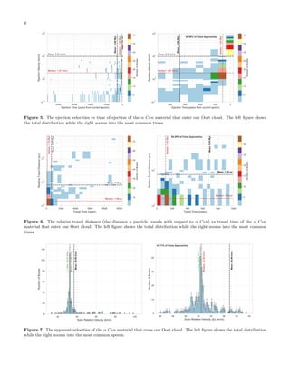
4
Table 1. The adopted values used to initialize our simulation, including the ICRS coordinates of α Centauri taken from
SIMBAD.
Parameter Units Value References
Mi, i = d, b, h 1010
M⊙ 7.91, 1.40, 69.80 [3]
ai, i = d, b, h pc 3500, 0, 0 [3]
bi, i = d, b, h pc 250, 350, 24000 [3]
r⊙ kpc 8.33±0.35 [4]
z⊙ pc 27±4 [2]
v⊙ (U, V, W) km s−1
(11.1+0.69
−0.75, 12.24+0.47
−0.47, 7.25+0.37
−0.36) [6]
v⊙,circ km s−1
218±6 [1]
Galactic Centre Equatorial Coordinates (α, δ) (hr:min:s, deg/’/”) (17:45:37.224, -28:56:10.23) [5]
α Centauri
Star System α µα δ µδ Parallax vr References
(deg) (mas yr−1
) (deg) (mas yr−1
) (mas) (km s−1
)
* alf Cen 219.873833 -3608 -60.83222194 686 742 -22.3 [7]
References— [1] Bovy (2015); [2] Chen et al. (2001); [3] Dauphole & Colin (1995); [4] Gillessen et al. (2009); [5] Reid
& Brunthaler (2004); [6] Schönrich et al. (2010); [7] Wenger et al. (2000)
We first simulate α Cen and the Sun backward from t = 0 (the current epoch) a total of 100 Myr, slightly less than
half of their galactic periods. From their positions and velocities at t ≈ −100 Myr, we allow the systems to progress
forward 110 Myr, ending t ≈ 10 Myr in the future, with a time step of ∼ 5000 yr. As we propagate the systems
forward again, their positions return to within the tolerance threshold at t = 0, the largest deviation observed being
7 × 10−5
au. As simulation time progresses, an additional 10,000 particles representing ejected material from α Cen
are added every 1 Myr. These particles play the role of both macroscopic telescopically observable km-class bodies
such as asteroids and comets, as well as smaller (sub-mm to m) sized particles that could be detected as meteors in
the Earth’s atmosphere.
2.2.1. Ejection model
Here we will assume that the particles ejected from α Cen leave the system with some excess velocity, but we will
not model their ejection in detail. Instead, we adopt a velocity distribution representative of the ejection process
plausibly at work in α Cen at the present time. Particles could be released by the gravitationally-driven ejection of
residual planetesimals by the multiple stars in the system (Bailer-Jones et al. 2018; Ćuk 2018; Smullen et al. 2016;
Jackson et al. 2018), or by known or unknown planets (Bailer-Jones et al. 2018; Brasser & Morbidelli 2013; Charnoz
& Morbidelli 2003; Correa-Otto & Calandra 2019; Duncan et al. 1987; Fernandez & Ip 1984; Portegies Zwart et al.
2018).
Bailer-Jones et al. (2018) produced an ejection speed distribution for the scattering of planetesimals by a giant
planet orbiting a single star, and by a binary star with masses 1 M⊙ and 0.1 M⊙. Though these parameters do not
exactly match α Cen’s, these models provide a reasonable first approximation to the speed distribution that we might
expect for planetary and stellar ejections. We adopt the binary star speed distribution (the red dashed line in Fig.
6 of Bailer-Jones et al. (2018)) as being most applicable here, and it is shown in Figure 1. Note that it includes a
low-velocity tail that covers the range of ejection speeds expected for planetary ejections as well, and indeed we will
see in Section 3 that low-speed ejections are favored in terms of reaching our Solar System.
This ejection speed is taken as the asymptotic speed with which the particles leave α Cen, v∞, and is multiplied
by a directional vector (chosen randomly from the surface of a unit sphere) and added to the velocity of the star to
determine the galactocentric velocity of the ejecta. The new ejected particle is placed within the simulation with the
same position as the origin system and with this new velocity vector.
Between each time step of integration, the minimum distance between any particle and the Sun is interpolated by
assuming a linear trajectory to avoid missing an encounter by stepping over it. If any particle passes within a specified

)UHTXHQF
0HDQ

N
P
V
0HGL
D
Q

N
P
V

(MHFWLRQ9HORFLWNPV

XPXO
D
WL
Y
H'L
V
WUL
E
XWL
R
Q)XQFWL
R
Q')

Figure 1. The ejection velocity distribution from our simulations, adapted from Figure 6 of Bailer-Jones et al. (2018) (their
red-dashed line). The right panel is our recreation of the Bailer-Jones et al. (2018) figure, showing the cumulative distribution of
ejection velocities caused from a binary star system with masses 1 M⊙ and 0.1 M⊙ on a circular orbit of with 10 au separation.
distance of the Sun (a heliocentric bubble of radius 100, 000 au, chosen more or less arbitrarily but representative of
the extent of the outer OC), the object is flagged as a close approach (CA), and all details are noted.
3. RESULTS
A total of 1.09×106
particles were ejected from the α Cen system throughout the simulation. As described in Section
2.2, the particles were ejected in random directions and their ejection speeds followed the distribution of Bailer-Jones
et al. (2018). The simulation began at t ≈ −100 Myr and ended at t ≈ 10 Myr (Figure 2 and the corresponding
animation).
Only a small fraction of the α Cen ejecta come within the CA distance of the Sun. In total, 350 particles had a
CA with the Solar System, ∼0.03% of the total ejecta. The first CA arrives at t ≈ −2.85 Myr. Material continues
to arrive for ∼ 10 Myr (Figure 3 and the corresponding animation) with the majority of CAs within ±200, 000 yr of
the current epoch (Figure 4). This peak is centered around α Cen’s time of closest approach to the Solar System in
∼ 28, 000 yr. In that figure we also include the effective cross-section of the Solar System (here taken to be of 105
au
radius) as viewed from α Cen and expressed as a solid angle. This cone reaches a maximum full-width of 37.5◦
when
α Cen is at its point of closest approach, and we see that the rate of arrivals broadly coincides with and peaks at
the same time. However, because the particle travel times are not zero, this is only an approximation of the effective
cross-section that they see and which depends on their relative velocity. Nevertheless, it illustrates that we expect
material to be transferred more efficiently as our Solar System’s apparent cross-section grows as we move towards our
point of closest approach with α Cen.
The ejection speed distribution from a giant planet peaks between 1 and 2 km s−1
(Bailer-Jones et al. 2018); while
in our simulations we find 52% of particles that arrive from α Cen have ejection speeds less than 2 km s−1
(with
a maximum around 77 km s−1
, Figure 5). Thus, the speeds that most effectively move material from α Cen to us
closely match those expected for ejection by a massive planet, such as might occur due to the planets around Proxima
Centauri, though no planets more massive than a mini-Neptune have yet been confirmed in the α Cen system.
The times of ejection (teject) that resulted in a CA ranged from teject ≈ −93 Myr to teject ≈ −12, 000 yr. The
majority of the CAs had ejection times closer to the current epoch (≈ 53% with teject −1 Myr; ≈ 84% with
teject −10 Myr), meaning that fresh ejecta was more likely to encounter the Solar System (Figure 5). This is as
expected, as the α Cen system is moving towards the Sun and the solid angle the Solar System subtends is largest when
their mutual distance is smallest. The majority (≈ 84%) of the CAs traveled for 10 Myr, a fraction of a galactic
orbit (Figure 6). These particles are therefore exposed to the ISM for a relatively short time, lessening any effects from

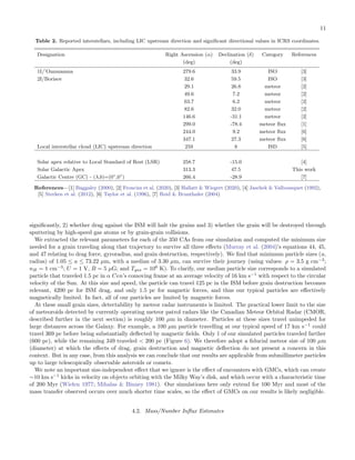
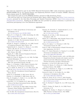
6
4000
3200
2400
1600
800
0
800
1600
2400
3200
4000
z
[pc]
24000
20000
16000
12000
8000
4000
0
4000
8000
12000
16000
20000
24000
x
[pc]
2800
2400
2000
1600
1200
800
400
0
400
800
1200
1600
2000
2400
z
rel
[pc]
8000
6000
4000
2000
0
2000
4000
6000
8000
10000
12000
14000
x
rel
[pc]
t=2,994 yr
Ejecta Positions Relative to Cen in Comoving Frame [pc]
Galactic Positions of Cen and 1,090,000 Ejecta [pc]
Figure 2. α Cen’s orbit about the Galactic Centre viewed on the xy and yz planes (top row), as well as the orbits of the
ejecta from α Cen viewed in a comoving frame (bottom row). Our Sun (Sol) is marked by a black hexagon and its orbital path
indicated by a grey solid line (top row only). α Cen’s location and path are shown by a yellow star and blue solid line (top
row only). In the bottom row, the comoving frame follows α Cen around its orbit while maintaining its orientation with the
y-axis pointing towards the Galactic Centre (blue arrow) and α Cen’s velocity pointing in the -x direction (black arrow). This
still frame is taken at t ≈ 3, 000 yr (that is, +3,000 years from the current epoch) after ∼ 100 Myr of integration. The colours
of the ejecta represent the 3rd dimension of position, except that any particle that will at any point come within 100, 000 au of
Sol are plotted in red. The full animation is available in the HTML version of this publication which shows the time evolution
from t ≈ −100 Myr to t ≈ 10 Myr. The duration of the animation is 11 s. https://youtu.be/YABoYgNKr-I
the galactic magnetic field, ISM drag, grain destruction, and perturbations from GMC encounters (discussed further
in Section 4.1).
When the CAs intercept the Solar System, their median apparent velocity relative to the Sun (∆v) observed at their
closest approach is 32.50 km s−1
, ranging from 13.75 km s−1
to 103.17 km s−1
(Figure 7). Due to the high fraction
of CAs that resulted from low ejection speeds, we see the solar relative velocities center around the current apparent
velocity of α Cen (∆v = 32.37 km s−1
) as expected.
As particles fall into the Solar System, their heliocentric speed vhel increases beyond the relative speed ∆v that they
have at large distances. If they are observed on Earth as meteors, their observed heliocentric speed will be given by
vhel =
s
∆v2 +
2GM⊙
r⊕
(4)

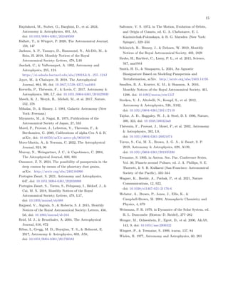
7
2800
2400
2000
1600
1200
800
400
0
400
800
1200
1600
z
rel
[pc]
8000
6000
4000
2000
0
2000
4000
6000
8000
10000
12000
14000
x
rel
[pc]
t=27,993 yr
Ejecta Positions Relative to Sol in Comoving Frame [pc]
Figure 3. The paths of the ejecta from α Cen viewed in a comoving frame with Sol. The comoving frame follows Sol around its
orbit maintaining the orientation with the y-axis pointing towards the Galactic Centre (blue arrow) and Sol’s velocity pointing
in the -x direction (black arrow). Our Sun (Sol) is indicated by a black hexagon and α Cen by a yellow star. This still frame
is taken at closest approach to our Solar System (t ≈ 28, 000 yr, years from the current epoch) after ∼ 100 Myr of integration.
The colours of the ejecta represent the 3rd dimension of position. The grey circle represents the extent of the Oort cloud
(100, 000 au), any particle that comes within this distance of Sol at any point is flagged as a close approach. These particles
are plotted in red. The full animation is available in the HTML version of this publication which shows the shower duration
from t ≈ −3 Myr to t ≈ 7 Myr. The duration of the animation is 44 s. https://youtu.be/qxd5kguXRWw
H H H H
$UULYDO7LPHHDUVIURPFXUUHQWHSRFK

1XPEHU
R
I

%
RGL
H
V
0HDQ

0
U
0HGL
D
Q

0
U

$UULYDO7LPHHDUVIURPFXUUHQWHSRFK

1XPEHU
R
I

%
RGL
H
V
0HDQ

HDUV
0HGL
D
Q

HDUV
RIORVH$SSURDFKHV

2RUW

O
R
XG
6
L
]
H

6RO
L
G

$
QJO
H

G
HJUHHV
2

Figure 4. The arrival times at the Solar System of the α Cen material. The left figure shows all close approaches while the
right zooms into the time of peak intensity. The green line shows the effective cross-section of the Solar System (the solid angle
subtended by our Oort cloud as seen from α Cen).
where ∆v is its velocity relative to the Sun when distant from our system and r⊕ is the Earth’s distance from the Sun.
Using our minimum, median, and maximum values found, we can determine an expected range of heliocentric speeds
in the inner Solar System, at 1 au from Sun, to be 44 ≲ vhel ≲ 111 km s−1
with a median around 53 km s−1
.
3.1. Meteor Radiants
The heliocentric equatorial radiant of CAs is plotted in Figure 8, and also plotted and animated for the resulting
“interstellar meteor shower” in Figure 9. The radiant would be the on-sky location from which the interstellar particle
would appear to originate if it appeared as a meteor in Earth’s sky. The figure converts the solar relative velocity

8
H H H H
(MHFWLRQ7LPHHDUVIURPFXUUHQWHSRFK

A Case Study of Interstellar Material Delivery: α Centauri

More Related Content

Similar to A Case Study of Interstellar Material Delivery: α Centauri

More from Sérgio Sacani

Recently uploaded

A Case Study of Interstellar Material Delivery: α Centauri