This thesis presents a benchmark suite for distributed stream processing systems to evaluate their performance across various applications and workloads. It addresses the need for comprehensive benchmarks, as existing ones cover only a limited range of applications, and proposes a framework to standardize application development and facilitate performance comparison. The research culminates in a validation of the benchmark through execution on multiple platforms, demonstrating its efficacy in aiding the selection of appropriate stream processing systems.

1. UNIVERSIDADE FEDERAL DO RIO GRANDE DO SUL
INSTITUTO DE INFORMÁTICA
PROGRAMA DE PÓS-GRADUAÇÃO EM COMPUTAÇÃO
MAYCON VIANA BORDIN
A Benchmark Suite for Distributed Stream
Processing Systems
Thesis presented in partial fulfillment
of the requirements for the degree of
Master of Computer Science
Advisor: Prof. Dr. Claudio Fernando Resin Geyer
Porto Alegre
May 2017

2. CIP — CATALOGING-IN-PUBLICATION
Bordin, Maycon Viana
A Benchmark Suite for Distributed Stream Processing Sys-
tems / Maycon Viana Bordin. – Porto Alegre: PPGC da UFRGS,
2017.
114 f.: il.
Thesis (Master) – Universidade Federal do Rio Grande do Sul.
Programa de Pós-Graduação em Computação, Porto Alegre, BR–
RS, 2017. Advisor: Claudio Fernando Resin Geyer.
1. Distributed systems. 2. Benchmark suite. 3. Stream pro-
cessing. 4. Real-time processing. 5. Big data. I. Geyer, Claudio
Fernando Resin. II. Título.
UNIVERSIDADE FEDERAL DO RIO GRANDE DO SUL
Reitor: Prof. Rui Vicente Oppermann
Vice-Reitora: Profa
. Jane Fraga Tutikian
Pró-Reitor de Pós-Graduação: Prof. Celso Giannetti Loureiro Chaves
Diretora do Instituto de Informática: Profa
. Carla Maria Dal Sasso Freitas
Coordenador do PPGC: Prof. Luigi Carro
Bibliotecária-chefe do Instituto de Informática: Beatriz Regina Bastos Haro

3. CONTENTS
LIST OF ABBREVIATIONS AND ACRONYMS........................................................5
LIST OF FIGURES.........................................................................................................6
ABSTRACT......................................................................................................................8
RESUMO..........................................................................................................................9
1 INTRODUCTION.......................................................................................................11
1.1 Motivation................................................................................................................11
1.2 Goals.........................................................................................................................12
1.3 Contributions...........................................................................................................12
1.4 Document Organization .........................................................................................13
2 EVENT-STREAM PROCESSING............................................................................15
2.1 Requirements...........................................................................................................15
2.2 Concepts...................................................................................................................16
2.3 History......................................................................................................................20
2.4 Operator Placement and Load Balancing ............................................................21
2.5 Fault Tolerance........................................................................................................24
2.6 Message Systems .....................................................................................................25
2.7 Platforms..................................................................................................................26
2.7.1 Storm......................................................................................................................26
2.7.2 S4 ...........................................................................................................................29
2.7.3 Spark Streaming.....................................................................................................30
2.7.4 Samza.....................................................................................................................32
2.7.5 Comparison............................................................................................................33
2.7.6 Other Platforms......................................................................................................34
2.8 Performance Evaluation.........................................................................................35
2.8.1 Benchmarks............................................................................................................35
2.8.2 SPS Comparisons...................................................................................................38
2.8.3 SPS Performance Tests ..........................................................................................39
2.8.4 Use Cases...............................................................................................................41
2.8.5 Benchmarks and Frameworks for CEP Systems....................................................41
2.8.6 Metrics ...................................................................................................................44
2.8.7 Evaluation of the Existing Benchmarks.................................................................45
2.9 Workload Characterization ...................................................................................46
2.10 Final Considerations.............................................................................................48
3 MODEL .......................................................................................................................52
3.1 Proposed Framework .............................................................................................52
3.1.1 Data Input...............................................................................................................53
3.1.2 Output ....................................................................................................................55
3.2 Methodology............................................................................................................56
3.2.1 Metrics ...................................................................................................................57
3.3 Application Selection ..............................................................................................59
3.4 Applications.............................................................................................................63
3.4.1 Word Count (WC)..................................................................................................63
3.4.2 Log Processing (LP) ..............................................................................................63
3.4.3 Traffic Monitoring (TM)........................................................................................64
3.4.4 Machine Outlier (MO)...........................................................................................65
3.4.5 Sentiment Analysis (SA)........................................................................................65
3.4.6 Spam Filter (SF).....................................................................................................67
3.4.7 Trending Topics (TT).............................................................................................67

4. 3.4.8 Click Analytics (CA) .............................................................................................68
3.4.9 Fraud Detection (FD).............................................................................................69
3.4.10 Spike Detection (SD)...........................................................................................69
3.4.11 Bargain Index (BI) ...............................................................................................70
3.4.12 Reinforcement Learner (RL)................................................................................72
3.4.13 Smart Grid Monitoring (SM)...............................................................................73
3.4.14 Telecom Spam Detection (VS) ............................................................................73
3.5 Workload Characterization ...................................................................................74
3.6 Configuration and Datasets....................................................................................76
4 RESULTS.....................................................................................................................82
4.1 Set-Up.......................................................................................................................82
4.2 Word Count .............................................................................................................83
4.3 Log Processing.........................................................................................................89
4.4 Traffic Monitoring ..................................................................................................96
4.5 Analysis of the Results..........................................................................................102
5 CONCLUSION .........................................................................................................104
REFERENCES.............................................................................................................105

5. LIST OF ABBREVIATIONS AND ACRONYMS
SMP Symmetric Multi-Processor
NUMA Non-Uniform Memory Access
SIMD Single Instruction Multiple Data
SPMD Single Program Multiple Data
ABNT AssociaÃ˘gÃˇco Brasileira de Normas TÃl’cnicas
SPS Stream Processing System
SPA Stream Processing Application
SPE Stream Processing Engine
ESP Event-Stream Processing
DSMS Data Stream Management System
CEP Complex Event Processing
IFP Information Flow Processing
CQ Continuous Query
PE Processing Element
ECA Event-Condition-Action
SQL Structured Query Language
DBMS Data Base Management System
ETL Extract/Transform/Load
DSL Domain Specific Language
VWAP Volume-Weighted Average Price
TAQ Trade And Quote

6. LIST OF FIGURES
Figure 2.1 Data stream and schema ................................................................................16
Figure 2.2 Types of parallelism in stream processing.....................................................19
Figure 2.3 Timeline of SPSs ...........................................................................................22
Figure 2.4 Replication of components ............................................................................24
Figure 2.5 Upstream backup ...........................................................................................25
Figure 2.6 Storm topology components and parallelism ................................................27
Figure 2.7 Example of a running topology in Storm ......................................................27
Figure 2.8 Storm cluster components .............................................................................28
Figure 2.9 Storm default scheduler.................................................................................28
Figure 2.10 Storm event tracking....................................................................................29
Figure 2.11 Structure of an S4 processing node .............................................................29
Figure 2.12 Example of application in Spark Streaming................................................31
Figure 2.13 Spark Components.......................................................................................31
Figure 2.14 A Samza Job executing a user-defined task.................................................32
Figure 2.15 Architecture of the Samza job execution on Hadoop YARN ......................33
Figure 3.1 Test Framework Architecture ........................................................................53
Figure 3.2 Relevance of application areas in the searched papers..................................62
Figure 3.3 Data flow of the Word Count application ......................................................63
Figure 3.4 Data flow of the Log Processing application.................................................64
Figure 3.5 Data flow of the Traffic Monitoring application............................................65
Figure 3.6 Data flow of the Machine Outlier application ...............................................65
Figure 3.7 Data flow of the Sentiment Analysis application ..........................................66
Figure 3.8 Data flow of the Spam Filter application.......................................................67
Figure 3.9 Data flow of the Trending Topics application................................................68
Figure 3.10 Data flow of the Click Analytics application...............................................69
Figure 3.11 Data flow of the Fraud Detection application..............................................70
Figure 3.12 Data flow of the Spike Detection application..............................................70
Figure 3.13 Data flow of the Bargain Index application.................................................71
Figure 3.14 Data flow of the Reinforcement Learner application. .................................72
Figure 3.15 Data flow of the Smart Grid Monitoring application...................................73
Figure 3.16 Data flow of the VoIPSTREAM application................................................74
Figure 3.17 Selectivity of operators................................................................................75
Figure 3.18 Tuple size per operator ................................................................................76
Figure 3.19 Memory usage per application (in MBytes)................................................77
Figure 3.20 Process time per tuple per operator .............................................................77
Figure 4.1 Cluster Azure.................................................................................................83
Figure 4.2 Storm Word Count Latencies.........................................................................84
Figure 4.3 Storm Word Count Best Latencies ................................................................84
Figure 4.4 Storm Word Count Throughput.....................................................................85
Figure 4.5 Storm Word Count Network Usage...............................................................85
Figure 4.6 Storm Word Count CPU and Memory Usage................................................86
Figure 4.7 Spark Word Count Latencies.........................................................................86
Figure 4.8 Spark Word Count Throughput .....................................................................87
Figure 4.9 Spark Word Count Network Usage ...............................................................87
Figure 4.10 Spark Word Count CPU and Memory Usage..............................................88
Figure 4.11 Storm Log Processing Latencies .................................................................89

7. Figure 4.12 Storm Log Processing Best Latencies .........................................................90
Figure 4.13 Storm Log Processing Throughput..............................................................90
Figure 4.14 Storm Log Processing Sink Throughput .....................................................91
Figure 4.15 Storm Log Processing Network Usage........................................................91
Figure 4.16 Storm Log Processing CPU and Memory Usage ........................................92
Figure 4.17 Spark Log Processing Latencies..................................................................93
Figure 4.18 Spark Log Processing Throughput ..............................................................93
Figure 4.19 Spark Log Processing Sink Throughput......................................................94
Figure 4.20 Spark Log Processing Network Usage ........................................................94
Figure 4.21 Spark Log Processing CPU and Memory Usage.........................................95
Figure 4.22 Storm Traffic Monitoring Latencies ............................................................97
Figure 4.23 Storm Traffic Monitoring Best Latencies ....................................................97
Figure 4.24 Storm Traffic Monitoring Throughput.........................................................98
Figure 4.25 Storm Traffic Monitoring Throughput without the Source Operator ..........98
Figure 4.26 Storm Traffic Monitoring Network Usage...................................................99
Figure 4.27 Storm Traffic Monitoring CPU and Memory Usage .................................100
Figure 4.28 Spark Traffic Monitoring Latencies...........................................................100
Figure 4.29 Spark Traffic Monitoring Throughput .......................................................101
Figure 4.30 Spark Traffic Monitoring Network Usage .................................................101
Figure 4.31 Spark Traffic Monitoring CPU and Memory Usage..................................102

8. ABSTRACT
Recently a new application domain characterized by the continuous and low-latency pro-
cessing of large volumes of data has been gaining attention. The growing number of
applications of such genre has led to the creation of Stream Processing Systems (SPSs),
systems that abstract the details of real-time applications from the developer. More re-
cently, the ever increasing volumes of data to be processed gave rise to distributed SPSs.
Currently there are in the market several distributed SPSs, however the existing bench-
marks designed for the evaluation this kind of system covers only a few applications and
workloads, while these systems have a much wider set of applications. In this work a
benchmark for stream processing systems is proposed. Based on a survey of several pa-
pers with real-time and stream applications, the most used applications and areas were
outlined, as well as the most used metrics in the performance evaluation of such appli-
cations. With these information the metrics of the benchmark were selected as well as a
list of possible application to be part of the benchmark. Those passed through a workload
characterization in order to select a diverse set of applications. To ease the evaluation
of SPSs a framework was created with an API to generalize the application development
and collect metrics, with the possibility of extending it to support other platforms in the
future. To prove the usefulness of the benchmark, a subset of the applications were ex-
ecuted on Storm and Spark using the Azure Platform and the results have demonstrated
the usefulness of the benchmark suite in comparing these systems.
Keywords: Distributed systems. benchmark suite. stream processing. real-time process-
ing. big data.

9. Um Benchmark Suite para Sistemas Distribuídos de Stream Processing
RESUMO
Um dado por si só não possui valor algum, a menos que ele seja interpretado, contextuali-
zado e agregado com outros dados, para então possuir valor, tornando-o uma informação.
Em algumas classes de aplicações o valor não está apenas na informação, mas também na
velocidade com que essa informação é obtida. As negociações de alta frequência (NAF)
são um bom exemplo onde a lucratividade é diretamente proporcional a latência (LOVE-
LESS; STOIKOV; WAEBER, 2013). Com a evolução do hardware e de ferramentas de
processamento de dados diversas aplicações que antes levavam horas para produzir resul-
tados, hoje precisam produzir resultados em questão de minutos ou segundos (BARLOW,
2013).
Este tipo de aplicação tem como característica, além da necessidade de processamento
em tempo-real ou quase real, a ingestão contínua de grandes e ilimitadas quantidades
de dados na forma de tuplas ou eventos. A crescente demanda por aplicações com esses
requisitos levou a criação de sistemas que disponibilizam um modelo de programação que
abstrai detalhes como escalonamento, tolerância a falhas, processamento e otimização de
consultas. Estes sistemas são conhecidos como Stream Processing Systems (SPS), Data
Stream Management Systems (DSMS) (CHAKRAVARTHY, 2009) ou Stream Processing
Engines (SPE) (ABADI et al., 2005).
Ultimamente estes sistemas adotaram uma arquitetura distribuída como forma de lidar
com as quantidades cada vez maiores de dados (ZAHARIA et al., 2012). Entre estes
sistemas estão S4, Storm, Spark Streaming, Flink Streaming e mais recentemente Samza
e Apache Beam.
Estes sistemas modelam o processamento de dados através de um grafo de fluxo com
vértices representando os operadores e as arestas representando os data streams. Mas
as similaridades não vão muito além disso, pois cada sistema possui suas particularida-
des com relação aos mecanismos de tolerância e recuperação a falhas, escalonamento e
paralelismo de operadores, e padrões de comunicação.
Neste senário seria útil possuir uma ferramenta para a comparação destes sistemas em
diferentes workloads, para auxiliar na seleção da plataforma mais adequada para um tra-
balho específico. Este trabalho propõe um benchmark composto por aplicações de di-
ferentes áreas, bem como um framework para o desenvolvimento e avaliação de SPSs

10. distribuídos.
Palavras-chave: sistemas distribuídos, benchmark suite, stream processing, processa-
mento em tempo-real, big data.

11. 11
1 INTRODUCTION
A data by itself holds no value unless it has been interpreted, contextualized and
aggregated with other data, then it has a value, which makes of it an information. In
some classes of applications the value is not only on the information, but also on the
speed with which it’s obtained. High Frequency Trading (HFT) is a great example of
applications where the profitability is directly proportional to the latency (LOVELESS;
STOIKOV; WAEBER, 2013). With the evolution of hardware and data processing tools
many applications that in the past took hours to give a response to a query, now need to
answer in a matter of minutes or seconds (BARLOW, 2013).
This kind of application has as a characteristic, beyond the need for real-time or
near real-time processing, the continuous ingestion of large and unbounded volumes of
data in the shape of tuples or events. The growing demand for applications that would
meet these requirements led to the creation of systems that provide a programming model
that take away from the programmer the responsibility with respect to details such as
scheduling, fault tolerance, processing and optimization of queries. These systems are
know as Stream Processing Systems (SPS), Data Stream Management Systems (DSMS)
(CHAKRAVARTHY, 2009) or Stream Processing Engines (SPE) (ABADI et al., 2005).
Lately these systems adopted a distributed architecture as a way to deal with ever
increasing volumes of data (ZAHARIA et al., 2012). Among them are S4, Storm, Spark
Streaming, Flink Streaming and more recently Samza and Apache Beam.
These systems model the data processing through a data flow graph with the ver-
tices being the operators and the edges the data streams. But the similarities don’t go
much further, as each of these systems has different mechanisms for fault tolerance and
recovery, scheduling and parallelism of operators, and communication patterns.
In this scenario it would be useful to have a tool for comparing these systems under
different workloads, to assist in the selection of the most suited for a specific job. We
propose a benchmark suite composed of applications from different fields of applications,
as well as a framework for the development and evaluation of distributed SPSs.
1.1 Motivation
Recently a new application domain characterized by the continuous and low-
latency processing of large volumes of data has been gaining attention. The growing

12. 12
number of applications of such genre has led to the creation of Stream Processing Sys-
tems (SPSs), systems that abstract details that have no direct relation to the problem at
hand.
More recently, the ever increasing volumes of data to be processed gave rise to
distributed SPSs. Currently there are in the market several distributed SPSs, however
the benchmarks that currently exist for these systems use only synthetic, very simple
applications or only applications from a few areas.Furthermore, benchmarks for other
types of Big Data systems, such as MapReduce, do use mostly real applications, as is the
case of BigDataBench ?? and HiBench ??.
1.2 Goals
The main goal of this work is the creation of a benchmark suite for SPSs composed
of real applications from different areas, workloads and data loads, defining metrics for
the measurement of the performance, scalability and reliability, and scenarios with the
occurrence of failures and bursts in the volume of data. With this benchmark suite we
expect to provide a reference point so that people interested in using an SPS can choose
the one that better fits its needs.
The second goal of this work is to create a framework for the execution of the
benchmark, as well as a low-level API for the unified development of applications, en-
abling applications to be written once and ran anywhere, as long as the driver for the
platform has been developed as well.
And a third goal is to apply the benchmark suite in a comparison between the main
distributed SPSs in the market. Through this comparison we expect to demonstrate the
usefulness of this benchmark suite, as well as provide a reference implementation of the
benchmark so that it can be applied in other SPSs.
1.3 Contributions
This research work expects to contribute with:
• Provide a set of real and meaningful benchmarks that can be reproduced.
The benchmarks are real and from diverse areas of applications, and their workload
has been characterized to ensure they have distinct behaviours. And the framework

13. 13
allows for applications to be executed on any supported platform, with the same set
of metrics and methodologies for its collection and summarization.
• Define a solid set of metrics for stream processing.
This work aims to research previous works, gather information on all metrics used
and then define the ones that are better suited for evaluating SPSs.
• Become a standard on SPS benchmarking.
Or at least improve the way these systems are evaluated, with higher quality bench-
marks that can better show how they perform in different scenarios.
• Provide a defined set of applications for benchmarking.
As well as a reference implementation for those applications, so that they can be
reproduced in other SPSs.
1.4 Document Organization
After this first Chapter, which contains a brief introduction of this research, the
rest of this document is organized as follows:
Chapter 2 introduces the basic concepts of Stream Processing on Sections 2.1 and
2.2. On Section 2.3 the history of Stream Processing and what came before it is described.
Then it moves to more specific areas of Stream Processing, such as operator placement
on Section 2.4, fault tolerance on Section2.5 and message systems on Section 2.6. We
introduce the main platforms of stream processing on Section 2.7 and then the main work
done in performance evaluation of these platforms on Section 2.8.
On Chapter 3 the model of this research is described, detailing the methodology
for benchmarking SPSs on Section 3.2, including the metrics that are going to be used for
evaluation of these systems. On Section 3.3 we describe how the selection of applications
took place and then on Section 3.4 we describe these applications in detail. In the end, at
Section 3.5, a workload characterization of these applications is described and finally the
configurations and datasets that can be used to execute these applications, on Section 3.6.
The results of the performance evaluation of Storm and Spark using a subset of
the applications of the benchmark are on Chapter 4. In Section 4.1 the set-up of the
environment is described, and in the subsequent sections the results of each application
evaluated are shown.
At last, in Chapter 5, are the conclusions of this research as well as the final con-

14. 14
siderations and future work.

15. 15
2 EVENT-STREAM PROCESSING
This chapter introduces the requirements and concepts that govern Stream Pro-
cessing Systems (SPSs), also known as Event-Stream Processing (ESP) or Stream Pro-
cessing Engines (SPEs), in Sections 2.1 and 2.2, respectively. Section 2.3 traces the his-
tory of SPSs back to the first Data Stream Management Systems (DSMSs), Complex
Event Processing systems (CEPs), Continuous Queries and Active Databases. In se-
quence, the architectural aspects of SPSs are explored, including techniques for schedul-
ing and load balancing jobs and tasks within jobs to Processing Elements (PEs) (Section
2.4), the methods employed for guaranteeing that messages are processed and the opera-
tor’s state is not lost in a failure (Section 2.5), as well as the different data transportation
middlewares and communication patterns used (Section 2.6).
In Section 2.7, the main platforms for stream processing are described in detail,
with the differences among them being highlighted. And lastly, the state of the art on
benchmarking and performance evaluation of SPSs is investigated (Section 2.8).
2.1 Requirements
Stream processing technologies have been created to fulfil a set of requirements
for a growing class of applications. Among these requirements, the most prominent is the
need for processing data in real time (or near real-time) and producing results in a timely
fashion.
In a paper by Stonebraker, Çetintemel and Zdonik (STONEBRAKER; ÇETINTEMEL;
ZDONIK, 2005), they also include as requirements the need to process data in-memory
in order to keep the latency low (1), the support for a high-level query language (2), the
ability to handle data imperfections (delays, missing and out-of-order data)(3), the gener-
ation of predictable and repeatable outcomes (4), the integration of real-time and stored
data (5), the guarantee of data safety and system availability (6), the automatic partition
and scalability of applications (7), and the last requirement is the one mentioned in the
beginning of this section.
To complement the requirements above, Chakravarthy (CHAKRAVARTHY, 2009)
also notes that an SPS has to be able to cope with the unpredictability of data stream rates
and also the large amount of data that may be required to be processed. Many applica-
tions have also very specific QoS requirements that must be met, such as response time

16. 16
(latency), precision, throughput and memory usage. The precision is regarding the results,
which means that some applications are willing to have approximate results in order to
increase or sustain other QoS requirements.
2.2 Concepts
The main abstraction of a SPS is the data stream. A stream is a continuous and
unbounded flow of data items arriving in some order (e.g. timestamp); the rate of ar-
rival may be fixed or unpredictable (e.g. tweets); with well-structured, semi-structured or
unstructured data. These data items are called tuples, events or messages, and they are
usually a set of key/value pairs. Tuples from the same data stream share the same data
schema, which describes its fields and respective data types (CHAKRAVARTHY, 2009).
Figure 2.1: Data stream and schema (BALAZINSKA, 2005)
Data streams are produced by external entities (in relation to the SPS) called data
sources. The data produced by a data source is made available for consumption through a
data pipeline, such as a socket, a file system or a more sophisticated message system. The
produced data is ingested by the SPS for processing through a component called source
or edge adaptor. This component receives the data in real-time and forwards it to the
downstream operators.
An operator, according to Andrade, Gedik and Turaga (ANDRADE; GEDIK;
TURAGA, 2014), is the basic functional unit of an application. An operator receives
as input one or more data streams, applies some function to a single tuple or a set of tu-
ples, and generates one or more output streams. Operators have input and output ports,
which are logical communication interfaces that allows them to receive and emit tuples to

17. 17
data streams, with each one port being associated to a single data stream.
Some of the more common tasks performed by operators are:
• Parsing/Filtering/ETL;
• Aggregation: collection and summarization of tuples;
• Merging: combining of streams with different schemas;
• Splitting: partitioning of stream into multiple ones for data/task parallelism of some
logical reason;
• Data mining/Machine Learning/Natural Language Processing: spam filtering, fraud
detection, recommendation systems, clustering, sentiment analysis;
• Others: relational algebra, artificial intelligence, computer vision, and other custom
operations.
According to Gulisano et al (GULISANO et al., 2010), operators can be classified
as stateless and stateful. Stateless operators only need the current tuple in order to produce
any results (e.g. map, filter), while stateful operators need more than one tuple (e.g.
join, aggregation). Stateful operators can be further classified as either blocking or non-
blocking. A non-blocking operator is one which, although storing data about past tuples,
can produce results after each new tuple processed.
A blocking operator, on the other hand, requires the whole dataset in order to
produce a result, such is the case of a join or frequent itemset operator. But since a data
stream is unbounded in size it is impossible for such operator to ever produce any results.
To overcome this restriction tuples can be grouped in windows based on a range of time
units or a number of tuples. Each window has a start (Ws), an end (We) and an advance
parameter (Advance). Different configurations for these parameters may create windows
of fixed or variable size, with or without overlap between windows (GULISANO, 2012).
Stream processing applications (SPAs) are also bound to other restrictions, such
as the limited processing time and memory, as they need to produce results in a timely
manner and to do so they must keep all data in memory, which is limited (and small if
compared to the hard disk), and the amount of processing lean. For some applications
these requirements were so important that they were willing to trade the accuracy of the
results for a smaller latency (time between ingestion of a tuple and production of results).
These approximate operators are usually based on synopsis structures (AGGAR-
WAL; PHILIP, 2007). The main examples of synopsis structures and their practical use
are:

18. 18
• Sampling: classification, query estimation, order statistics estimation, distinct value
queries;
• Wavelets: hierarchical decomposition and summarization;
• Clustering: knowledge discovery;
• Sketches: distinct count, heavy hitters, quantiles, change detection;
• Histograms: range queries, selectivity estimation.
On the other end of an application is the data sink, which is similar to a normal
operator, except for the fact that it does not produce any output streams. A data sink has
the purpose of exporting the results of a SPA, either to a database or to another system,
for visualization or further processing.
In stream processing an application is usually composed as a flow graph with
nodes as operators and directed edges as data streams and the communication follows the
publish-subscribe model. There are, however, different programming models for stream
processing:
• DAG (Directed Acyclic Graph): a directed graph without cycles.
• Actors model: an actor is a computational entity that can respond to a message by
sending messages to other actors, creating new actors and designating the behaviour
for the next message it receives, all in parallel.
• Monad: originated from functional programming, it is a structure that represents a
chain of operations.
The parallelism of SPAs (Figure 2.2) can be expressed in three ways: pipeline,
data or task parallelism. The pipeline parallelism works similarly to the way a CPU
processes instructions, with instructions being analogous to operators. In order for task
parallelism to work properly an application must have the right level of decomposition, in
order to accomplish a good usage of computational resources.
Data parallelism consists on the execution of the same task over different data
items or Single Instruction Multiple Data (SIMD). This type of parallelism depends on the
nature of the operator: stateless, partitioned-stateful or stateful. Obviously, the simpler
case lies in the stateless operators, because the workload can be evenly distributed among
their instances without any worries about dependencies between tuples. With partitioned-
stateful operators, however, some sort of consistency must be followed when splitting a
data stream among an operator’s instances. With stateful operators simply choosing a par-
titioning configuration is not enough, it usually involves operators dedicated specifically

19. 19
for splitting, merging and re-ordering the tuples.
The most common partitioning configurations are:
• Shuffling: tuples are randomly and evenly distributed.
• Group By: tuples are distributed accordingly to the value of one or more fields.
• Broadcast: the entire data stream is replicated to all subscribers.
• Directed: tuples are distributed directly to a selected subscriber.
Figure 2.2: Types of parallelism in stream processing (ANDRADE; GEDIK; TURAGA,
2014)
At last, the task parallelism is closely related to the nature of SPAs, as they are a
composition of tasks that, in many cases, work in parallel. But even if the task parallelism
is almost unavoidable in an SPA, it is paramount to ensure the balance between these tasks
in order to improve the performance and avoid waste of resources, such as extra memory
usage due to large queues of tuples waiting to be merged.
Another important aspect of SPSs is the way the processing of tuples is carried
out. The first approach used is the record-at-a-time, which means that each tuple is pro-
cessed by the operators individually, providing a very low latency. There are however
two main downsides of this approach: lower throughput and high overhead for tracking
message delivery. To overcome these shortcomings some SPSs process data streams in
mini-batches (MURALIDHARAN; KUMAR; BHASI, 2014), which tends to increase the
throughput, at the cost of an increase in latency. It also means that the system needs only
to track the delivery of the batches instead of individual tuples.

20. 20
2.3 History
Stream Processing is only one among a series of systems developed for processing
large volumes of data in real-time and giving information to act upon in a timely manner,
all of them part of what is called Information Flow Processing (IFP). The early IFP sys-
tems helped pave the way to the modern SPSs in the market which, according to Andrade,
Gedik and Turaga (ANDRADE; GEDIK; TURAGA, 2014), are:
• Active databases rely on ECA (Event-Condition-Action) rules in order to capture
events, the surrounding conditions and the actions to be taken in case the conditions
are met. Current DBMSs implement these active database features with triggers
defined using SQL.
• Continuous Queries are known as standing queries as opposed to relational database
queries (snapshot queries), because they continuously monitor incoming informa-
tion, producing a stream of results. A CQ is composed of a query, a trigger which
will activate the query, and a stop condition which will determine when the query
should stop to compute updates.
• Publish-subscribe system is composed of publishers that produce data and sub-
scribers that consume that data in the form of messages. The components of a
pub-sub system have no knowledge of each other, and the delivery of message lies
upon a broker network composed of brokers nodes. There are two categories of
pub-sub systems defined accordingly to how consumers subscribe to data.
In a topic-based pub-sub system, consumers simply subscribe to topics and receive
all data produced by publishers in those topics, a characteristic that simplifies the
routing of messages within the broker network. With a content-based pub-sub sys-
tem however, the routing is much more complex, because each message must be
evaluated in order to determine to which subscribers it is going to be delivered.
Each publication has a set of properties and each subscription defines a set of con-
ditions based on these properties.
• Complex Event Processing systems collect, filter, aggregate, combine and corre-
late events originated from multiple sources in order to create more complex events
and/or take action based on the detected events (ROBINS, 2010).
According to Heinze et al (HEINZE et al., 2014), the history of SPSs can be broken
in three generations:

21. 21
In the first generation, systems were devised to work in a single node (centralized)
with applications developed using query languages derived from SQL, but continuous
instead of snapshot-based, or visual languages (boxes and arrows). The use of SQL as
foundation happened in some cases because these systems were using relational database
engines underneath.
Among the first SPSs developed the most notable are the TelegraphCQ, developed
at the University of California, Berkeley; STREAM, developed at Stanford University;
and Aurora, developed by a collaboration between the Brandeis University, Brown Uni-
versity and MIT.
The second generation went a step further, with systems working on very large
networks, mainly for processing data from sensor networks, which means that the pro-
cessing must occur in a distributed fashion.
In this period a lot of research was built on all aspects surrounding SPSs, such as
job and resource management, scheduling, load balancing, high availability, monitoring,
fault tolerance, QoS, visualization, stream algorithms and query languages. In comparison
with the the first generation, now the systems have a much wider range of operators, as
well as the ability to build custom operators. Examples from this generation are: Borealis,
CEDR, System S and CAPE.
In the third generation there is a shift towards massively-parallel systems, working
on clusters instead of very large networks. These systems also favor general purpose
languages instead of DSLs (Domain Specific Languages), giving the developer a wide
range of possibilities for building applications. The focus is now on processing large
volumes of data as fast as possible using clusters of computing nodes, usually with Cloud
Computing. Examples from the third generation are: S4, Storm, Spark Streaming, Flink
Streaming, Samza and Apex.
2.4 Operator Placement and Load Balancing
Meeting QoS requirements is not an easy task as it usually involves balancing
aspects that most of the time work against each other. In a environment where data can
present bursts of volume, a system has to be able to cope with it, while maintaining the
established QoS.
In an SPS, the operators of a query will be spread across multiple computing
nodes, thus meeting the QoS requirements means finding a good operator placement and

22. 22
Figure 2.3: Timeline of SPSs (HEINZE et al., 2014)(VINCENT, 2014)
since stream loads can greatly vary along time, these systems should also employ good
load balancing techniques.
The processing graph is considered the logical representation of the query which
will be used by the scheduler in the placement of operators. The mapping of operators to
computing nodes will create the physical representation of the query, where the vertices
now represent the nodes (KOSSMANN, 2000; RUNDENSTEINER; LEI; GUTTMAN,
2013).
One of the main differences in the way the scheduler works depends on the type
of load partitioning supported by the system (JOHNSON et al., 2008). Data stream
partitioning allows an operator to be placed in several nodes, distributing the load among
them. Whereas in query plan partitioning one operator can live only in one node, with
the disadvantage that if an operator consumes more resources then a machine can offer,

23. 23
the only solution is to upgrade the machine or apply some technique of admission control.
Following the taxonomy defined by Casavant and Kuhl (CASAVANT; KUHL,
1988) another important aspect of schedulers for DSPSs is the time at which the operator
placement is made (statically or dynamically). Giving the variable nature of data streams
most schedulers proposed in the literature approach the problem with a initial operator
placement and an online load balancing, with special attention to the management of
bursts.
More recently a taxonomy was proposed (LAKSHMANAN; LI; STROM, 2008)
specifically for SPSs. The authors propose six core components that describe placement
algorithms:
• Architecture: whether is an independent module from the system, a distributed
one with each node executing an instance of it, or an hybrid of both approaches.
• Algorithm Structure: if the algorithm has knowledge of the entire network’s state
it is centralized, otherwise it is decentralized, using only local knowledge to make
decisions.
• Metrics: used in the objective functions in order to optimize the placement of oper-
ators. Commonly used metrics are the load, latency, bandwidth, machine resources
and operator importance.
• Operator-Level Operations: describes the operations supported by the operators
in order to improve the performance of the operator placement algorithm, such
as reusing an operator that appears in more than one query (operator reuse) and
replicating one operator to improve the performance (replication).
• Reconfiguration: ability of the algorithm to adapt in order to cope with changes in
the network, input rate or application components.
• Response Strategies: some algorithms requires the application to stop in order for
a new placement to be calculated, while other algorithms can dynamically respond
to changes by migrating operators or redistributing the load among the operators or,
if possible, using some technique such as load shedding.
• Change Triggers: operator migration can be triggered if certain performance thresh-
old has been trespassed, a constraint has been violated, or by periodically checking
if the gain from migrating an operator is greater that the cost of moving it.

24. 24
2.5 Fault Tolerance
Fault tolerance in SPSs is of utmost importance due to the fact that its applications
have to run for large periods of time. An SPS can suffer from node crashes and partitions,
component and networks failures.
It has to guarantee that the state of the system is consistent and that all messages
received are processed. In order to accomplish that some techniques can be employed.
In the next paragraphs the main techniques, according to Gradvohl et al (GRADVOHL et
al., 2014), will be described.
Replication of components, as the name suggests consists of replicating a com-
ponent of the system so that in case of a failure the replicated component can take over the
failed one. The replication can happen actively, meaning that the replicated component
receives the same input as the main component, and in case of a failure the replicated
component can take over immediately. The drawback is that the cost of the component
is also duplicated. The other approach is the passive replication, and in this case the
replicated component is dormant, and in case of a failure all the input processed by the
failed component has to be replayed to the replicated component. Depending on the size
of the input to be replayed the time required for the component to reach the same state
as the failed component can be intolerable. To overcome this, the technique that will be
described next can be used.
Figure 2.4: Replication of components (HEINZE et al., 2014)
Operator
Operator
Operator
Previousstage
Nextstage
State
State
State
Data
State implicitly synchronized by
ordered evaluation of same data
Active replication
Operator
Operator
(dormant)
Operator
(dormant)
Previousstage
Nextstage
State
State
State
Data
State periodically persisted on stable
storage and recovered on demand
Passive replication
Checkpoints
Checkpointing consists of saving the state of the system periodically to a stable
storage, enabling the recovery of the state in case of a failure. Checkpoints can be unco-

25. 25
ordinated, with each process deciding when to make the checkpoint, which can lead to
system inconsistencies; or coordinated, where all processes agree on when to checkpoint,
thus requiring the exchange of messages between them.
Figure 2.5: Upstream backup (BALAZINSKA; HWANG; SHAH, 2009)
Upstream backup requires a node to save the tuples it is sending to downstream
nodes in a queue until the downstream nodes have processed them (ack messages). In
case of a failure the node can send the tuples again. It can become a problem if the size
of the queue grows outside the main memory.
Recovery is classified as precise, when all tuples not processed by the downstream
nodes are sent, the failure is completely masked (except for the delay in processing); on
roll-back recovery the output may be different from that of a failure-free execution as
some tuple may be duplicated; and in gap recovery some tuples may be lost in order to
reduce the recovery time.
2.6 Message Systems
According to Bockermann (BOCKERMANN, 2014) a queueing or message pass-
ing component is one of the two main functionalities of an SPS, the other being the execu-
tion engine itself. The message system will be responsible for connecting the components
of an SPS, transporting tuples from producers to consumers, ensuring that the connections
are fault-tolerant and are performing well regarding throughput and latency (ANDRADE;
GEDIK; TURAGA, 2014).
Systems such as S4 used to rely solely on TCP, changing later to the Netty library.
Storm did something similar, changing from ZeroMQ to Netty. And while these systems
rely on libraries to handle their communication, some systems prefer to use a middleware,
as is the case of Apache Samza which uses Kafka as its message system. Other examples
of middlewares are RabbitMQ and ActiveMQ.

26. 26
2.7 Platforms
In this section the most prominent SPSs in the open source market are described.
It is assumed that the basic concepts of stream processing are known (Section 2.2). The
descriptions focuses mainly o programming and architectural characteristics. At the last
section there is a qualitative comparison of the platforms, highlighting their similarities
and differences.
2.7.1 Storm
Storm is an open source distributed real-time computation system. Applications
are called topologies and they are built as DAGs, with spouts as data sources and bolts
as operators, the communication between these components happens through streams.
Each component can declare the streams, and their respective schemas, that he is going to
produce, however, only bolts can subscribe to streams.
The data parallelism is provided by Storm through what is called stream grouping.
By default there are seven options:
1. Shuffle grouping: tuples are random and evenly distributed among bolt’s tasks.
2. Fields grouping: tuples are grouped by the specified fields, meaning that tuples
with the same value for the grouping field will always go to the same task.
3. All grouping: all tasks receive all the tuples, i.e. the stream is replicated.
4. Global grouping: the entire stream goes to the task with the lowest ID.
5. None grouping: currently it is the same as the shuffle, but eventually it will try to
put the subscriber task in the same thread as the publisher.
6. Direct grouping: the publisher of the tuples chooses the task to which the tuple
will be sent.
7. Local or shuffle grouping: if the subscriber has one or more tasks in the same
worker process as the publisher, the tuples will be shuffled only among them, oth-
erwise it will act just like a normal shuffle.
The parallelism of each component is defined at declaration, as seen in Figure
2.6. In Storm this is the number of executors or threads that will be spawned for each
component by a worker, which is a process that resides in one machine of a Storm cluster

27. 27
and runs executors of one topology. Executors run one or more tasks, which are the ones
that perform the data processing.
Figure 2.6: Storm topology components and parallelism (HEINZE et al., 2014)
Spout
Spout
Spout
Spout
Bolt Bolt
Bolt
BoltBolt
Bolt
Bolt
Bolt
x3
x8
x5
In Figure 2.7 it is possible to see an example of a running topology with two
workers, one spout configured with two executors and two tasks, a green bolt with two
executors and four tasks, and a yellow bolt with six executors and six tasks.
Figure 2.7: Example of a running topology in Storm (Apache Storm, 2014)
A Storm cluster (Figure 2.8) is composed of one Nimbus (the master) and a set of
supervisors (the workers). The Nimbus is responsible for assigning work to supervisors,
as well as starting and stopping workers accordingly; managing failures; and monitor-
ing resource usages (HEINZE et al., 2014). Supervisors have a parameter called slots,
which is the maximum number of workers that they can execute (ANIELLO; BALDONI;
QUERZONI, 2013). The coordination between the Nimbus and the supervisors relies on
a Zookeeper cluster. Moreover, all state of the nodes is kept on Zookeeper in order to
avoid data loss in case of a failure, enabling nodes to restart after a failure and continue
from where they left off (Apache Storm, 2014).

28. 28
Figure 2.8: Storm cluster components (HEINZE et al., 2014)
When the Nimbus receives a topology it has to use a scheduler in order to assign
executors to workers and workers to slots (ANIELLO; BALDONI; QUERZONI, 2013).
The default scheduler of Storm (EvenScheduler, Figure 2.9) employs a round robin strat-
egy for the assignment of executors to workers.
Figure 2.9: Storm default scheduler (HEINZE et al., 2014)
Storm guarantees that all messages emitted by the spouts will be fully processed
by keeping them on a queue until the confirmation that they have been processed, and
in case a message has failed the spout will send it again (GRADVOHL et al., 2014).
To understand what "fully processed" means in Storm a simple example can be seen in
Figure 2.10, it shows the tuple tree which is composed of the original tuple and all tuples
originated from that first tuple. After a tuple is processed in a bolt it is ack’ed, after all
tuples in the tuple tree have been ack’ed the message is considered fully processed.

29. 29
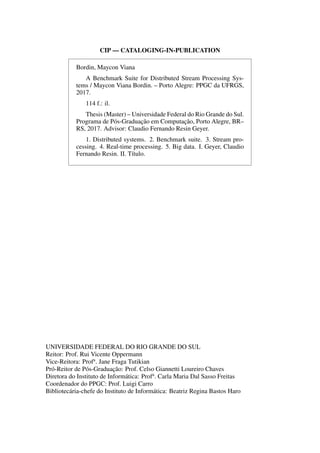
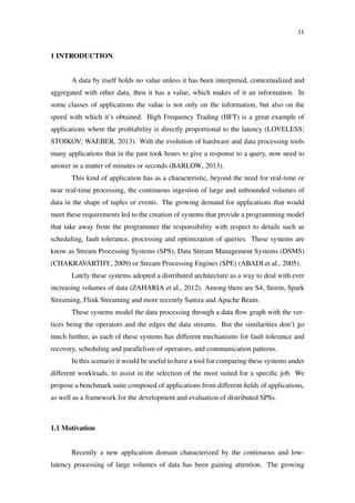
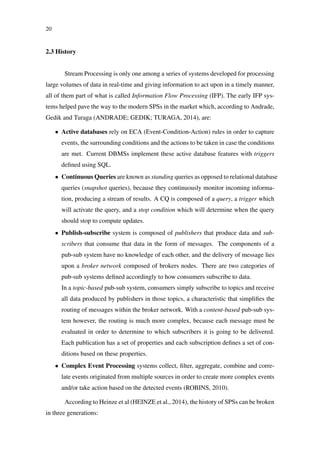
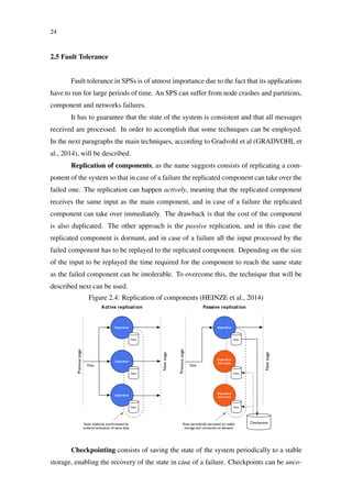
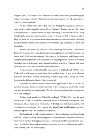
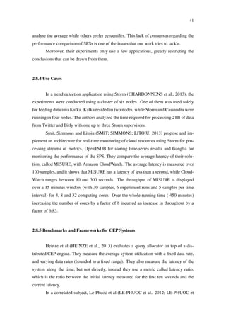
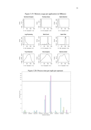
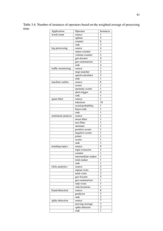
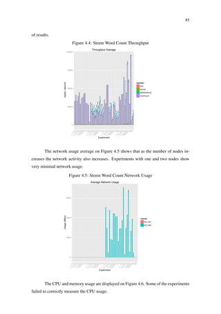
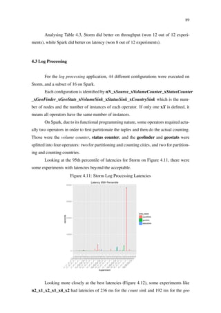
Figure 2.10: Storm event tracking (HEINZE et al., 2014)
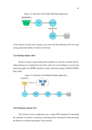
Spout
Splitter
bolt
Counter
bolt
“stay hungry, stay foolish”
text lines words
[“stay”,“hungry”,“stay”,“foolish”] [“stay”, 2]
[“hungry”, 1]
[“foolish”, 1]
“stay hungry, stay foolish”
“stay” [“stay”, 1]
“hungry”
“stay”
“foolish”
[“hungry”, 1]
[“foolish”, 1]
[“stay”, 2]
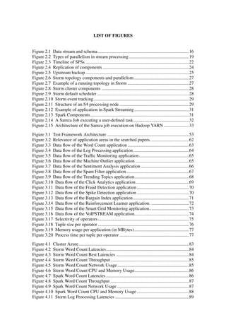
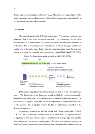
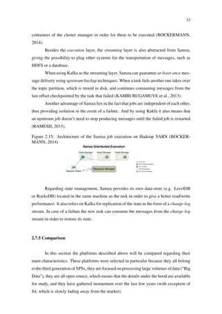
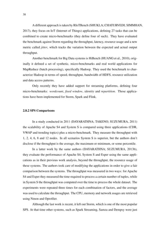
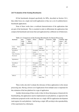
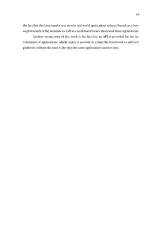
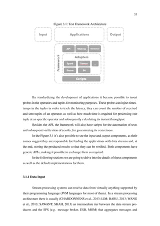
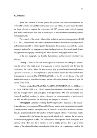
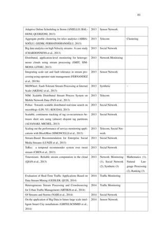
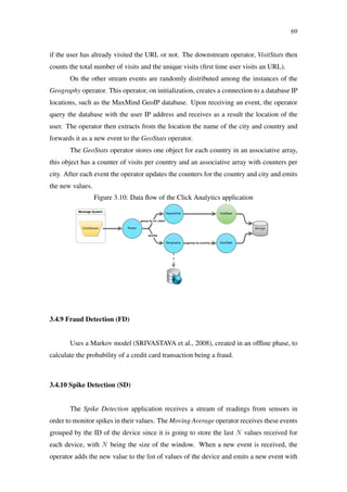
2.7.2 S4
S4 is a framework for distributed stream processing based on the Actors model.
Applications are built as a graph composed of processing elements (PEs) that process
events and streams that interconnect the PEs. Events are made of a key and a set of
attributes, and they are forwarded to a PE based on the value of the key, with exception of
keyless PEs.
In fact, the parallelism of S4 is based on event keys. Each key value will create a
new instance of an PE, meaning that large key domains will generate a large number of PE
instances. An S4 application is deployed in an S4 cluster composed of containers called
S4 nodes (see Figure 2.12) that execute PEs from multiple applications. These nodes
are coordinated using Apache Zookeeper and the communication between nodes happens
through TCP connections. One drawback of S4 is that a cluster has a fixed number of
nodes, meaning that to create a cluster with more nodes it is necessary to create a new S4
cluster.
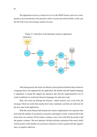
Figure 2.11: Structure of an S4 processing node (BOCKERMANN, 2014)
4.3 S4 – Distributed Stream Computing Platform
The S4 platform is a distributed stream processing framework that was initially developed
at Yahoo! and has been submitted to the Apache Software Foundation for incubation into
the Apache Software Repository. It is open sources under under the Apache 2 license.
Note: According to the Apache incubator report of March 2014, S4 has considered to
be retiring from incubation as the community is inactive and development efforts have
deceased.
The S4 system uses a cluster of processing nodes, each of which may execute the processing
elements (PE) of a data flow graph. The nodes are coordinated using Apache Zookeeper.
Upon deployment of a streaming application, the processing elements of the application’s
graph are instantiated at various nodes and the S4 system routes the events that are to
be processed to these instances. Figure 17 outlines the structure of a processing node in
the S4 system.
Each event in the S4 system is identified by a key. Based upon this key, streams can
be partitioned, allowing to scale the processing by parallelizing the data processing of
a single partitioned stream among multiple instances of processing elements. For this,
two types of processing elements exist: keyless PEs and keyed PEs. The keyless PEs can
be executed on every processing node and events are randomly distributed among these.
The keyed processing elements define a processing context by the key, which ensures all
events for a specific key to be routed to that exact PE instance.
The messaging between processing nodes of an S4 cluster is handled using TCP connec-
tions.
Processing Node
PE1 PE2 PEn
Event
Listener
Dispatcher Emitter
Figure 17: The structure of an S4 processing node executing multiple processing elements
(PEs). A node may execute the PEs of various applications.
Execution Semantics & High Availability
S4 focuses on a lossy failover, i.e. it uses a set of passive stand-by processing nodes
which will spawn new processing elements if an active node fails. No event buffering or
Regarding fault tolerance, S4 detects node failures using Zookeeper and reassign
tasks to other nodes (BOCKERMANN, 2014), passive stand-by processing nodes to be
exact, a technique called lossy failover (KAMBURUGAMUVE et al., 2013). The mes-

30. 30
sage semantics guarantees only at-most-once processing, which means that events may
be lost as no buffering or acknowledgement of events is provided (gap recovery).
S4 does however have a state management mechanism that periodically check-
points the state of PEs to a backend storage. In case of a failure the reassigned task will
load the last checkpointed state.
2.7.3 Spark Streaming
Spark Streaming is a stateful distributed stream processing system, part of the
Apache Spark cluster computing framework. One key difference of this platform is the
way it handles data streams, with events being processed in batches of fixed time intervals
instead of a record-at-a-time (Apache Spark, 2014).
Batches are also treated as Resilient Distributed Datasets (RDDs), a data structure
that keeps data in memory and can be recovered without the need of replication. Instead
it tracks the lineage graph of operations applied in order to build it, something possible
since the computations are deterministic (ZAHARIA et al., 2013).
In Spark Streaming streams are called D-Streams (discretized streams), sequences
of immutable and partitioned RDDs, with deterministic operations applied at them to
create new D-Streams.
The framework follows the monad programming model. The API provides func-
tionality for reading input data from outside the system in order to create the initial D-
Stream. There are two types of operations that can be applied to D-Streams: transforma-
tions and output operations. The framework provides the basic stateless operations com-
monly seen in batch processing frameworks (and functional programming languages), in
addition to windowing operations, incremental aggregations and state tracking.
An application is what can be called a D-Stream Graph, analogous to the dataflow
graph discussed in Section 2.2. At each batch interval the RDD graph is computed from
the D-Stream graph, each output operation will create a Spark action which will in turn
create a Spark job to compute the interval.
Spark Streaming can recover from failures by using RDDs. The input data is
replicated in memory and in case of a failure an RDD partition can be recomputed by
applying the transformations that built it to the input data. It also checkpoints the state of
RDDs periodically to an external storage (e.g. HDFS), and the recovery can be performed
in parallel.

31. 31
Figure 2.12: Example of application in Spark Streaming that reads input data from Twitter
Streaming API, extract the hashtags and saves them on an external storage (e.g. HDFS).
batch @ t+1batch @ t batch @ t+2Twitter Streaming API
flatMap flatMap flatMap
…
tweets DStream
hashTags Dstream
*#cat, #dog, … +
save save save
Figure 2.13: Spark Components
Worker
Task execution
Block manager
Input receiver
Worker
Task execution
Block manager
Input receiver
replication of
input & check-
pointed RDDs
Client
Client
Master
Task scheduler
Block tracker
RDD lineage
D-Stream lineage
Input tracker
Comm. Manager
Comm. Manager
New
Modified
(a) Components (ZAHARIA et al., 2013)
Execution Model – Receiving Data
Spark Streaming + Spark Driver Spark Workers
StreamingContext.start()
Network
Input
Tracker
Receiver
Data recvd
Block
Manager
Blocks replicated
Block
Manager
Master
Block
Manager
Blocks pushed
(b) Data Reception (DAS, 2013)
Spark Workers
Execution Model – Job Scheduling
Network
Input
Tracker
Job
Scheduler Spark’s
Schedulers
Receiver
Block
Manager
Block
Manager
Jobs executed on
worker nodes
DStream
Graph
Job
Manager
JobQueue
Spark Streaming + Spark Driver
Jobs
Block IDsRDDs
(c) Job Scheduling (DAS, 2013)
Its architecture (Figure 2.13 (a)) consists of three main components: a master
that manages the lineage graph of D-Streams and schedules tasks to compute new RDD
partitions; the worker nodes that receive data, store the partitions of input and computed
RDDs and execute tasks; and the client library that sends the data into the system.
In Spark the component responsible for receiving data from the network is the
Network Receiver (Figure 2.13 (b)), when it receives data it launches tasks in the workers
in order for transfer it to them. The Receiver then push the data blocks to the Block
Manager, the block will also be replicated and the Receiver will notify the master that
the blocks have been received and send to the Block Manager Master the location of the
block IDs.
The Job Scheduler (Figure 2.13 (c)) periodically queries the D-Stream graph in
order to create the jobs for the received data for the batch intervals. These jobs are stored

32. 32
in a queue by the Job Manager, also responsible for sending them to the Spark Scheduler
for execution in the worker nodes.
2.7.4 Samza
Samza is a framework for distributed stream processing built around Kafka. In
Samza an operator is a job, it can subscribe and publish to one or more streams. The par-
allelism is defined by the number of partitions of the Kafka’s topic that the job subscribes
to (if multiple topics, the one with more partitions).
A job is then broken down into tasks, each one responsible for consuming data
from one or more partitions, that operates independently of each other (RAMESH, 2015).
These tasks will be executed by Task Runners.
As a job is the equivalent of a single operator, more complex data flows can be cre-
ated by submitting more jobs to Samza, connected only by their input and output streams.
This particular characteristic makes it possible to change a data flow without stopping the
application.
Figure 2.14: A Samza Job executing a user-defined task with two input streams, each with
two partitions.
The architecture of Samza is divided in three layers: processing, execution and
streaming. While Samza is responsible for processing the data, the execution (distribu-
tion, scheduling and coordination) of tasks lies upon a cluster manager such as Apache
Mesos or Apache YARN (RAMESH, 2015). Samza places the Task Runners inside the

33. 33
containers of the cluster manager in order for them to be executed (BOCKERMANN,
2014).
Besides the execution layer, the streaming layer is also abstracted from Samza,
giving the possibility to plug other systems for the transportation of messages, such as
HDFS or a database.
When using Kafka as the streaming layer, Samza can guarantee at-least-once mes-
sage delivery using upstream backup techniques. When a task fails another one takes over
the topic partition, which is stored in disk, and continues consuming messages from the
last offset checkpointed by the task that failed (KAMBURUGAMUVE et al., 2013).
Another advantage of Samza lies in the fact that jobs are independent of each other,
thus providing isolation in the event of a failure. And by using Kakfa it also means that
an upstream job doesn’t need to stop producing messages until the failed job is restarted
(RAMESH, 2015).
Figure 2.15: Architecture of the Samza job execution on Hadoop YARN (BOCKER-
MANN, 2014)
Execution Semantics & High Availabilty
As Samza uses Kafka as message broker2
, all messages are stored on disk, providing per-
sistence of the streams consumed and produced by Samza’s stream tasks. This allows
for a restart of failed tasks by resuming at the last valid position in the data stream that
is provided by Kafka. Building on top of Kafka, Samza does provide an at-least-once se-
mantic for the processing of messages. Any further message guarantees (i.e. exactly-once)
requires custom handling, e.g. by keeping track of duplicates and discarding messages
that have already been processed.
Instead of implementing its own, fault tolerant process execution engine (i.e. like Storm),
Samza provides a context for its jobs by means of Task Runners and uses the Hadoop
YARN platform to distribute and execute these Task Runners on a cluster of machines.
Hadoop YARN is a continuation of the Apache Hadoop framework and provides a high-
level cluster API of loosely coupled machines. Worker machines in such a YARN cluster
run a Node Manager process which registers to a central Resource Manager to provide
computing resources. A YARN application is then a set of executing elements that are
distributed among the Node Manager processes of the cluster machines. Hadoop YARN
provides abstract means for handling fault tolerance by restarting processes.
For executing a Samza job, the job elements are provided to a Samza Application Master
(AM), which is allocated by requesting the Resource Manager to start a new instance
of the AM. The AM then queries the registered Resource Managers to create YARN
containers for executing Samza Task Runners. These Task Runners are then used to run
the Stream Tasks of the Samza job. As the allocation of distributed YARN containers
is provided by the Resource Manager, this results in a managed distributed execution of
Samza jobs completely taken care of by Hadoop YARN.
Samza Distributed Execution
Samza Client
job
Resource Manager
Node Manager Node Manager Node Manager
AM
Samza Job
Samza Application Master
Yarn Container
Yarn Node Manager
Yarn Resource Manager
Figure 15: Architecture of the Samza job execution on Hadoop YARN. The Samza client
requests the instantiation of an Application Master, which then distributes copies of the
task of a Samza job among YARN containers.
Scalability and Distribution
A Samza job that is defined by a Stream Task T and connected to an input stream I will
result in the parallel execution of multiple instances of the job task T for distinct parts
2
Use of Apache Kafka as message broker is the default setting. Samza claims to support different
messaging systems as replacement.
25
Regarding state management, Samza provides its own data-store (e.g. LevelDB
or RocksDB) located in the same machine as the task in order to give a better read/write
performance. It also relies on Kafka for replication of the state in the form of a change-log
stream. In case of a failure the new task can consume the messages from the change-log
stream in order to restore its state.
2.7.5 Comparison
In this section the platforms described above will be compared regarding their
main characteristics. These platforms were selected in particular because they all belong
to the third generation of SPSs, they are focused on processing large volumes of data ("Big
Data"), they are all open source, which means that the details under the hood are available
for study, and they have gathered momentum over the last few years (with exception of
S4, which is slowly fading away from the market).

34. 34
Table 2.1 summarizes the main characteristics of these platforms. These character-
istics were found in the documentation of the respective platforms and in previous works
(BOCKERMANN, 2014; GRADVOHL et al., 2014; KAMBURUGAMUVE et al., 2013)
that compared some of these platforms.
Most of the characteristics used for the comparison have been described in Section
2.2, considering that they are some of the building blocks of SPSs. Others however, are
more specific or technical and as such they will be detailed in the following paragraphs.
The distributed cluster characteristic refers to the support of the platform for
working in multiple computers as a distributed system, something that all the platforms
compared have. Directly related to the previous characteristic, the stream partitioning
represents the data partitioning features of the platforms, something necessary in order
to parallelize SPAs among nodes in a cluster. The difference is the way the partitioning
is implemented, and among these platforms Storm is the one with the widest range of
options.
Rebalacing is the capacity to rebalance the executing processes among the com-
puting nodes in order to cope with changes in the load. Together with a dynamic cluster,
i.e. the ability to add new nodes to a running cluster, it is possible to scale an application
as it requires more resources in order to honor the application’s QoS requirements.
Dynamic graph is the ability to make changes in an application (add or remove
operators) without having to restart it.
Regarding the communication characteristics, the message system refers to the
middleware or library used to create the channels between the components of an applica-
tion, whereas the data mobility indicates if the components control the flow rate (pull) of
messages or not (push).
The delivery guarantees on the other hand are closely related to the fault toler-
ance mechanisms implemented by the platforms, topic approached in Section 2.5. The
values for the available guarantees are: EO (exactly once), AMO (at most once), ALO (at
least once), OO (out of order).
2.7.6 Other Platforms
In the last three years a lot of platforms have been created or gained a lot of atten-
tion. Among those Flink and its streaming module is one of the most prominent. It is an
open source distributed batch and stream processing platform. It’s streaming engine has

35. 35
the record-at-a-time processing model with exactly-once delivery guarantees and support
for state persistence.
Among the open-source platforms that appeared in the last few of years are: Apache
Apex, a YARN-native platform that unifies batch and stream processing; Apache Beam, a
programming model for building and executing batch and stream applications in a num-
ber of supported platforms (Apex, Spark, Flink and Google Cloud Dataflow); Apache
Gearpump, a event/message based stream processing engine based on Akka; Apache Ig-
nite, a streaming and continuous event processing engine with focus on scalability and
fault-tolerance; hazelcast-jet, a distributed data processing engine that works on top of
Hazelcast; Heron, a distributed stream processing engine created by Twitter to replace
Storm, with a fully compatible API (WINGERATH et al., 2016).
2.8 Performance Evaluation
Of interest of this work are benchmarks specifically designed for SPSs, compar-
isons between SPSs, performance tests of new SPSs, use cases of applications that em-
ploy an SPS and perform some experiments to evaluate it, sometimes comparing against
a traditional solution; and benchmarks and frameworks from CEP systems, due to the
similarities that exist between these two areas.
In the end, in Section 2.8.6, a summary of the metrics employed by each of the
related works is given, as a way to find a consensus.
2.8.1 Benchmarks
The first benchmark designed specifically for stream processing systems that can
be found in the literature is the Linear Road Benchmark (ARASU et al., 2004b), adopted
by the Aurora (ABADI et al., 2003) and STREAM (ARASU et al., 2004a) systems. It
simulates a toll system in a fictitious city with the purpose of calculating the toll value
based on traffic jam and accident proximity, charging drivers greater values when there’s
more congestion as a way to discourage them from using the roads. In this simulation
there are express ways composed of four lanes, with vehicles reporting their position every
30 seconds and accidents happening in random locations every 20 minutes. The purpose
of the benchmark is to determinate the maximum L factor (number of express ways) that

36. 36
a system can process without violating the response time and precision requirements. The
queries defined by the benchmark are: accident detection, traffic congestion measurement,
toll calculation and historical queries. At the end of the paper a comparison between
a relational DBMS and Aurora is presented, with a measured L factor of 0.5 and 2.5,
respectively.
Besides the Linear Road Benchmark, there are benchmarks for SPSs that are
aimed at very specific cases, as is the case of PLR (KARACHI; DEZFULI; HAGHJOO,
2012) which is an extension of the Linear Road for probabilistic DSMSs, and the SR-
Bench (ZHANG et al., 2012) that defines a set of queries for the comparison of Streaming
RDF/SPARQL (strRS) engines.
The first benchmark suite for the 3rd generation of SPSs is StreamBench (LU
et al., 2014). It proposes a set of seven applications for the workload, based on three
dimensions of requirements for stream processing: data type, workload complexity and
use of historical data. The benchmark also defines four aspects that are going to be
measured: performance, with the input rate at its maximum with four input scales (5M,
10M, 20M and 50M); multi-recipient performance, where the input scale is fixed but the
number of nodes in the cluster that receive the input data varies (single node, half of the
nodes and all nodes of the cluster); fault tolerance, with half of the nodes as recipients, it
consists on failing one non-recipient node and measuring the performance under failure
and comparing to a failure free experiment; durability, uses only one application with
10K and 1M records per minute during 2 days, and measures the percentage of available
time of the framework.
The applications that compose the benchmark suite are: identity, sample, projec-
tion, grep, word count, distinct count and statistics. Six of them work with text data
types and one with numeric data type, four of them have only a single operator and are
stateless. One shortcoming of this benchmark suite is that all applications are synthetic,
leaving aside more complex operations and communication patterns that only occur with
more complex data flow graphs. It’s worth noting that the authors acknowledge this fact.
The datasets used by the benchmark suite are from real world scenarios and they
use them as seed for data generation. The seed data should be pre-loaded in memory in
order to increase the performance as the data generation speed should be superior to the
data consumption. The generated data, according to the proposed architecture, is feeded
into a message system, decoupling the data generation from data consumption. It is also
necessary that the message system should have a serving speed superior from the con-

37. 37
sumption speed. The authors claim that even if the SPSs could achieve greater throughput
without a message system, by being the common data transport for all experiments it
results in a fair comparison.
As most of the works below, they chose the average throughput and latency as
main metrics, and the penalties incurred from failures in this two metrics. They have
done experiments to compare Storm and Spark Streaming in a cluster of 6 nodes, using
Apache Kafka as the message system in a cluster of 6 nodes, with 5 of them as brokers.
They fail, however, to present the standard deviation of the results measured, something
essential for the comparison of systems known for their high variability in latency and
throughput.
Another benchmark for SPSs was Yahoo Streaming Benchmark (Yahoo Storm
Team, 2015), composed of an Ad campaign stream application and implementations for
Storm, Spark, Flink and Apex systems. They analyze the throughput and 99th percentile
of latency on those platforms with their default set-up configurations. Results showed that
Storm had a great performance and a throughput almost as good as Flink and with some
optimizations it could achieve an even better performance.
A later work on benchmarking Big Data systems is BigDataBench (WANG et al.,
2014), with a wide range of applications from multiple areas. It also has a subset of
five micro-benchmarks specific for streaming systems: grep, search, rolling top words,
k-means and collaborative filtering (for e-commerce).
It provides the specification of all benchmark applications as well as the data in-
puts, but it is not a framework in the sense that it does not provide an API that can be
extended for building new benchmarks. The micro-benchmarks have been implemented
for JStorm and Spark.
Another work specific for SPSs is StreamBench (WANG, 2016) (not the same
as (LU et al., 2014)), an extensible framework for the evaluation of these systems. The
benchmark defines three micro-benchmarks: AdvClick, for clickstream analysis with
correlation between ads and clicks on those ads; WordCount; and K-Means, applied to
a stream of points with a pre-defined set of centroids.
The benchmark provides implementations of those applications for Storm, Spark
and Flink, using the latency and throughput as evaluation metrics. One downside of the
framework is the fact that applications need to be implemented for each platform sepa-
rately. In addition, these applications do not represent real world and complex applica-
tions, and they don’t use realistic inputs.

38. 38
A different approach is taken by RIoTBench (SHUKLA; CHATURVEDI; SIMMHAN,
2017), they focus on IoT (Internet of Things) applications, defining 27 tasks that can be
combined to create micro-benchmarks (they define four of such). They have evaluated
the benchmark against Storm regarding the throughput, latency, resource usage and a new
metric called jitter, which tracks the variation between the expected and actual output
throughput.
Another benchmark for Big Data systems is HiBench (HUANG et al., 2010), orig-
inally it defined a set of synthetic, micro-benchmarks and real world applications for
MapReduce (batch processing), specifically Hadoop. They used the benchmark to char-
acterize Hadoop in terms of speed, throughput, bandwidth of HDFS, resource utilization
and data access patterns.
Only recently they have added support for streaming platforms, defining four
micro-benchmarks: wordcount, fixed window, identity and repartition. Those applica-
tions have been implemented for Storm, Spark and Flink.
2.8.2 SPS Comparisons
In a study conducted in 2011 (DAYARATHNA; TAKENO; SUZUMURA, 2011)
the scalability of Apache S4 and System S is compared using three applications (CDR,
VWAP and trending topics) plus a micro-benchmark. They measure the throughput with
1, 2, 4, 6, 8 and 12 nodes. In all scenarios System S is superior, but the authors don’t
disclose if the throughput is the average, the maximum or minimum, or some percentile.
In a latter work by the same authors (DAYARATHNA; SUZUMURA, 2013b),
they evaluate the performance of Apache S4, System S and Esper using the same appli-
cations as in their previous work analysis, beyond the throughput, the resource usage of
these systems. The authors took care of modifying the applications in order to give a fair
comparison between the systems. The throughput was measured in two ways: for Apache
S4 and Esper they measured the time required to process a certain number of tuples, while
in System S the throughput was computed over the time to process the whole dataset. The
experiments were repeated three times for each combination of factors, and the average
was used to calculate the throughput. The CPU, memory and network usages are retrieved
using Nmon and Oprofiler.
Although the last work is recent, it left out Storm, which is one of the most popular
SPS. At that time other systems, such as Spark Streaming, Samza and Dempsy were just

39. 39
in its infancy, but it means that there is no comparison between these systems in the
literature, nor even in white papers or technical reports.
2.8.3 SPS Performance Tests
In the Spark Streaming platform (ZAHARIA et al., 2012) they measure the maxi-
mum throughput achievable of the system with 1s and 2s of maximum latency for different
cluster sizes. They also introduce node failures and measure the processing time for each
job, before and after the failure.
In an evaluation of the performance of Apache S4 (CHAUHAN; CHOWDHURY;
MAKAROFF, 2012) a single application is used to observe its scalability, resource us-
age and fault tolerance. For the scalability analysis they use as factors the number of
nodes in the cluster (1 to 3), data size (10 and 100 megabytes), input rate (500 and 1000
events/sec), and number of keys. The metrics are the total number of events processed
(50k times number of keys) and the number of events lost. They do not use runtime as a
metric because an under provisioned setup would lead to high tuple loss and small run-
times, giving the false impression that using one node is better than two or more. The
resource usage is depicted for each node of the cluster with the CPU and memory usage,
while the network usage is summarized for the whole cluster and measured in packets per
second. The experiments that evaluate the fault tolerance of Apache S4 were conducted
by killing one (in a 2-node and 3-node cluster) and two (in a 3-node cluster) nodes lead-
ing, as expected, to a reduction in throughput, overwhelming the remaining nodes and
thus leading to higher tuple losses.
For MillWheel (AKIDAU et al., 2013), a distributed and fault tolerant SPS devel-
oped at Google, the main metric used to evaluate it is the latency. Regarding its scalability,
they look at the median, 95th and 99th percentiles. Results show that while the latency
median remains almost unchanged, the tail gets longer.
Another distributed SPS called TimeStream (QIAN et al., 2013) is evaluated re-
garding its scalability, fault tolerance, consistency and adaptability to load dynamics.
TimeStream packs events into batches for transportation, by varying the batch size they
measure the maximum throughput and latency with a distinct count application. They
pick five batch sizes and measure the throughput and latency with different number of
computing nodes and compare it with Apache Storm. In a sentiment analysis application
they use a dataset of 1.2 billion tweets, feeding the system at a rate of 600 tweets/s in

40. 40
average, with a peak of 2,000 tweets/s. To evaluate the fault tolerance of TimeStream the
authors use the same two applications. With the distinct count they only inject a failure
in one of the computing nodes and observe the recovery time for different window sizes
and checkpointing intervals. For the sentiment analysis application they inject failures by
selecting operators that form a chain in the DAG and killing one, three or the whole chain
of operators and measuring the recovery time for each operator.
Fernandez et al (FERNANDEZ et al., 2013a) implement a scalable SPS that ex-
poses operator’s internal state for checkpointing and backup purposes. For their experi-
ment they use dedicated VM instances (with large RAM memory available) to emit the
data streams and receive the results. Their system is able to scale as a result of an increas-
ing input rate. The latencies observed were very skewed for the Linear Road Benchmark,
as a result, the authors chose to use the 99th and 95th percentiles, besides the median. The
authors also observe the time required for an operator to recover after the willful failure
of the VM hosting the operator.
In the evaluation of Watershed (RAMOS et al., 2011), a distributed SPS, a com-
posed application for analysis of tweets is employed. The first experiment received data
at a fixed rate of 10 tweets/s with the number of instances of one operator (stopwords
remover) varying from 1 to 24. In this experiment only the throughput is measured over
a runtime of 2 minutes. In a second experiment, 10M tweets are pushed to the system
through a single instance of the collector operator (a spout), while the other operators of
the application have the number of instances ranging from 1 to 7. This time they measure
the execution time and calculate the speedup, but they don’t repeat their experiments.
The largest experiment in terms of computing infrastructure for a SPS was done
by (GULISANO, 2012). They used a cluster of 100 nodes to evaluate the scalability and
elasticity of StreamCloud, the distributed SPS the authors had proposed. Their evaluation
focus on the system’s ability to harness the computing power available to process an
increasing number of tuples. This ability is translated into the metrics of throughput and
CPU usage. The authors also evaluate the throughput and CPU usage for fixed number of
nodes, breaking down the metrics per operator. All the experiments were run three times,
and the measurements were taken in the steady phase of the running time, which lasted at
least 10 minutes.
These works were important in the selection of metrics and methodologies for the
benchmark suite. There are some similarities among them, mainly regarding latency and
throughput, although the way they have chosen to look to these metrics differs, some

41. 41
analyse the average while others prefer percentiles. This lack of consensus regarding the
performance comparison of SPSs is one of the issues that our work tries to tackle.
Moreover, their experiments only use a few applications, greatly restricting the
conclusions that can be drawn from them.
2.8.4 Use Cases
In a trend detection application using Storm (CHARDONNENS et al., 2013), the
experiments were conducted using a cluster of six nodes. One of them was used solely
for feeding data into Kafka. Kafka resided in two nodes, while Storm and Cassandra were
running in four nodes. The authors analyzed the time required for processing 2TB of data
from Twitter and Bitly with one up to three Storm supervisors.
Smit, Simmons and Litoiu (SMIT; SIMMONS; LITOIU, 2013) propose and im-
plement an architecture for real-time monitoring of cloud resources using Storm for pro-
cessing streams of metrics, OpenTSDB for storing time-series results and Ganglia for
monitoring the performance of the SPS. They compare the average latency of their solu-
tion, called MISURE, with Amazon CloudWatch. The average latency is measured over
100 samples, and it shows that MISURE has a latency of less than a second, while Cloud-
Watch ranges between 90 and 300 seconds. The throughput of MISURE is displayed
over a 15 minutes window (with 30 samples, 6 experiment runs and 5 samples per time
interval) for 4, 8 and 32 computing cores. Over the whole running time ( 450 minutes)
increasing the number of cores by a factor of 8 incurred an increase in throughput by a
factor of 6.85.
2.8.5 Benchmarks and Frameworks for CEP Systems
Heinze et al (HEINZE et al., 2013) evaluates a query allocator on top of a dis-
tributed CEP engine. They measure the average system utilization with a fixed data rate,
and varying data rates (bounded to a fixed range). They also measure the latency of the
system along the time, but not directly, instead they use a metric called latency ratio,
which is the ratio between the initial latency measured for the first ten seconds and the
current latency.
In a correlated subject, Le-Phuoc et al (LE-PHUOC et al., 2012; LE-PHUOC et

42. 42
al., 2013) proposes a framework for the evaluation of LSD engines (Linked Stream Data,
e.g. RDF stream data model). Their work includes a methodology for data generation,
system testing and analysis of results. The tests defined by the framework fall into one of
the three categories: functionality, correctness and performance tests. Functionalities are
covered through queries of increasing complexity, and the results assert if the functionality
is supported by the engine or not. The correctness tests evaluates the output of a query
for all engines given the same input and configuration. In cases of mismatch between
the outputs of different engines, a function for calculating the percentage of mismatch is
employed. In the performance tests the main metric is throughput, but in the case of LSD
engines, as the input rate increases the system may drop some tuples (load shedding),
which could lead to wrong results. To circumvent this problem, the authors proposed the
comparable maximum execution throughput.
Similar to the work described above, (SCHARRENBACH et al., 2013) gives a
few insights into how to benchmark SFP (Semantic Flow Processing, i.e. LSD engines)
systems. Of interest to this work is the three KPIs they have defined, they are: the re-
sponse time, measured by the average, xth percentile or the maximum; maximum input
throughput per unit of time; and other metrics including recall (reprocessing a lost tuple),
precision and error rate.
In 2007, Bizarro (BIZARRO, 2007) proposed the BiCEP project, a benchmark for
CEP engines. The paper identified the categories of applications for CEP engines based
on publications from a few conferences. It also defined a set of metrics: response time;
scalability, broken down into scale-up (increase system and load), speed-up (increase
system, maintain load) and load-up (maintain system, increase load); adaptivity, which
observes the behaviour of the engine in the face of changes in input rate, bursts in event
arrival, system overloads and instability; computation sharing, that evaluates the ability
of the engine to have multiple queries running concurrently; precision and recall.
In continuation to the BiCEP project, Mendes, Bizarro and Marques (MENDES;
BIZARRO; MARQUES, 2008) developed a framework for the performance evaluation of
CEP systems called FINCoS. The framework is language-agnostic, in the sense that it can
be used with any CEP product; and workload-agnostic, enabling the use of any dataset
and queries to evaluate a set of engines. The architecture of the framework is composed
of drivers that simulate streams of events, sinks that are going to receive the output from
the CEP engine, the controller used by the user to configure the environment (number of
drivers and sinks, rate of events, number of machines), the adapters that translate the input

43. 43
and output between the CEP engine and the standard format, and the validators that check
the output results as well as performance metrics (e.g. response time).
In a subsequent paper, the same authors put in practice their FINCoS framework
(MENDES; BIZARRO; MARQUES, 2009) using a set of micro-benchmarks to compare
the performance of three CEP engines (Esper and other two commercial engines). Their
benchmarks focus on simple operations (windowing, transformation, filtering, sorting,
grouping, merging, join, pattern detection) using as factors the content of the dataset,
window configurations, event rate, and number of queries (not all factors are used for a
single benchmark). Just like the work by Gulisano et al (GULISANO, 2012), they also
wait for the engine to warm-up before starting to measure the performance, for at least
ten minutes, depending on the application. Experiments were repeated two times with the
average being used. Most benchmarks use the throughput as their metric. In two cases
were the size of the window is a factor they also measure the memory consumption with
different input rates, window sizes and number of queries.
In another set of experiments their aim was to observe the engine’s performance
in the face of a burst. Like in the other experiments, the execution consisted of a warm-
up period of one minute in which the input rate was increased to λ such that the CPU
utilization were around 75%; in a steady phase of five minutes the rate was kept at the
λ rate; then during 10 seconds the injection rate was increased to 1.5λ; and finally in a
recovery phase the original input rate of λ was restored. To characterize the performance
of the engine the following metrics were introduced: maximum peak latency, the maxi-
mum latency during or immediately after the peak load; peak latency degradation ratio,
the ratio between the 99th percentiles of the latency in the peak phase and in the steady
phase; recovery time, which is the amount of time necessary for the engine to return to
the latency level of the steady phase after a peak; and post-peak latency variation ratio,
which is the ratio between the average latency after recovery and the steady phase.
Wahl and Hollunder (WAHL; HOLLUNDER, 2012) proposed an environment for
the comparison of CEP engines, focusing on the interchangeability of engines, repro-
ducibility and comparability of the test scenarios and automation of test execution and
measurement. They defined three test scenarios: latency test, which creates four events
that are emitted to the CEP engine to create a complex event, and once this result event is
received the latency is calculated; pollution test, based on a defined CEP rule, events that
fall into the rule are generated as well as events that don’t, the rate of events is constant,
but the number of irrelevant events is increased and the latency, CPU load and memory

44. 44
usage are monitored; and the load test that increases the number of event emitters and
observes the same parameters as the previous test.
The most recent work on CEP benchmarking is CEPBen (LI; BERRY, 2014),
which is both a benchmark as well as a framework. One key difference of this work is
that the smallest unit of data is not an event, but a batch of events. In practice there are
three factors that can be changed in the workload: the number of batches, i.e. the size of
the dataset; the size of the batch; and the interval between batches, i.e. the input rate. As
most benchmarks, the CEPBen also uses as metrics the throughput, subdivided into input
and output throughput, and the response time, i.e. (end-to-end) latency.
The authors of CEPBen define, instead of full-fledged applications, three groups
of tests based on functionalities that are the building blocks of event processing: filtering,
transformation and event pattern detection. The factors that weigh in the experiments
are, besides the workload, the number of query statements, as more statements means
more operations that need to be performed for each event; the amount of historical events
needed by the query, as it means more memory needs to be used to store these events; and
of course, the hardware where the CEP engine is running.
The framework developed for running the benchmarks is very similar to previous
works described here, with components for data generation and adaptation, event con-
sumers that receive the results, and the components for monitoring, storing and analysing
the engine’s metrics. At the end of the paper they present a performance study using their
benchmark with the Esper CEP engine.
2.8.6 Metrics
The Table 2.2 summarizes the metrics used by the works cited in the sections
above. The metric that appears the most is scalability, followed by throughput and latency.
The runtime is not so popular, mainly because SPAs in the real world usually don’t have
a limited execution time. The tuple loss and recovery time metrics are used in works that
study the tolerance of SPSs to faults.

45. 45
2.8.7 Evaluation of the Existing Benchmarks
Of the benchmarks designed specifically for SPSs, described on Section 2.8.1,
they either focus on a single real-world application or they use a set of synthetic/micro-
benchmark applications.
None of these works does a workload characterization of the applications that
are part of the benchmark. This is essential in order to differentiate the applications that
compose the benchmark and ensure that each application has a different set of behaviours.
Table 2.3: Comparison of the Existing Benchmarks for Stream Processing
Benchmark Real
World
Appli-
cations
Synthetic
/ Micro-
benchmarks
Metrics Platforms Framework Single
API
Workload
Charac-
teriza-
tion
Single
API
Level
Linear Road
Benchmark
1 - Aurora,
STREAM
No No No -
StreamBench
(2014)
- 7 Throughput,
Latency
Storm, Spark No No Yes -
Yahoo Streaming
Benchmark
1 - Throughput,
Latency
Storm,
Spark, Flink,
Apex
Yes No No -
BigDataBench - 5 JStorm,
Spark
Yes No No -
StreamBench
(2016)
- 3 Throughput,
Latency
Storm,
Spark, Flink
Yes Yes No High
RIoTBench - 4 Throughput,
Latency,
Resource
Usage,
Jitter
Storm No No Yes -
HiBench - 4 Latency Storm,
Spark, Flink
Yes No No -
These works also don’t evaluate the relevance of those applications in the stream
processing area. Having a diverse set of applications from multiple areas is important for
the evaluation of the best platform for a type of application.
Another shortcoming of these works is that, for those that propose a framework for
benchmarking, the applications need to implemented on each platform, as opposed to the
architecture proposed on this work that aims at a single API for application development
(and engines for each platform). And having a single API can help in the reproducibility
of the experiments by a third party.

46. 46
2.9 Workload Characterization
According to Bienia et al (BIENIA et al., 2008) the relevance of a benchmark suite
depends on the applications selected, as they need to represent the most significant use
cases as well as a broad and diverse range of behaviours.
The characterization of applications therefore plays a key role in the selection of
the workloads of a benchmark suite. In a paper by Balaprakash et al (BALAPRAKASH
et al., 2013), three techniques are employed in the characterization of applications: per-
formance measurement, instrumentation and source code analysis. They use them to
determine the instruction mix and memory access patterns for a set of scientific applica-
tions and extrapolate the results for exascale workloads per statistical models. Application
characteristics can also be obtained from traces of production environments (KHAN et al.,
2012).
The first step in the workload characterization of SPAs is to determine which as-
pects should be observed, taking into account that they must be relevant regarding its
influence in the performance of a SPS.
In the literature these aspects are usually explored in scheduling algorithms, as
they estimate the cost of an application and build an execution plan, seeking the best use
of resources while guaranteeing the QoS of the application.
In a paper by Bai and Zaniolo (BAI; ZANIOLO, 2008) the authors propose an
scheduling algorithm that is able to reduce the latency and memory consumption with
results very close to the optimal. The importance of memory usage was already acknowl-
edged by the early schedulers for DSMSs, e.g. Chain scheduler (BABCOCK et al., 2003).
Thus, the memory usage is one important aspect of an application that has to take part in
the characterization criteria.
Wei et al (WEI et al., 2006) presents a QoS management scheme that analyses
applications, predicts application workloads and adjusts the QoS levels to increase the
system utility. As part of their work, they analyse the cost of operators, in particular the
selection and join operators. Generalizing their analyses to expand any operator, the as-
pects observed in an operator to estimate its cost are: the input size in number of tuples,
n; the selectivity of the operator, s = size(output)/size(input), which can be the aver-
age for a filter(-like) operator (BABCOCK et al., 2004); the time to do the operation, Co;
and the time to send the output tuple, Ci, which could be zero depending on the message
system.

47. 47
Ideally, one of the aspects that characterize a stream processing application is the
input rate, as some applications may have more steady input rates while others present
a bursty nature. Instead, we decided to use the input rate as a factor in the experiments,
submitting all the applications to the same rates, both steady and bursty.
Regarding the input size, as we are dealing with a data stream, which is unbounded
by nature, there’s no reason to use it to characterize applications. The selectivity of the
operator, on the other hand, is very important, as it set volume of traffic for the down-
stream operators. With s > 1, for example, the operator will be increasing the volume of
tuples sent to the downstream operators. The selectivity of operators was also used in the
Chain scheduler (BABCOCK et al., 2003) as parameter for generating query plans.
Besides the aspects that directly influence the performance of an SPS, there are
other aspects that characterize an application and should be considered as they distin-
guish one application from another. These aspects are more concerned in describing
the different features displayed by these applications, much in the same way that (BAL-
APRAKASH et al., 2013) used the operation-type composition of the applications.
In stream processing there are two basic aspects that characterize an application:
the operator type and the communication pattern. The types of operators are those from
the relational algebra, such as selection, projection, join and aggregation. For more com-
plex operators, like the frequent itemset, a composition o relational algebra operators
would have to be employed, in this case an aggregation with group by.
As for the communication patterns, in an SPS an operator can basically send1
a
tuple to all subscribers (broadcast), to a random subscriber (shuffle), always to the same
subscriber based on values of the tuple (group by) or to a specific subscriber (see Section
2.2).
This is a very high-level characterization of the communication pattern, one that
can be realized through source code analysis. But there is a more detailed characterization,
obtained by means of instrumentation, that describes the temporal, spatial and volume
attributes of the communication (KIM; LILJA, 1998), obtained by the observation of the
distributions of message generation rates, message destinations, and message sizes and
average number of messages, respectively.
1
At the description of the application it is the subscriber who actually chooses the communication pat-
tern, but at runtime the pattern is usually employed at the publisher.

48. 48
2.10 Final Considerations
In this chapter we introduced the basic requirements and concepts of Event-Stream
Processing, a brief history of Stream Processing Systems, the main techniques for opera-
tor placement, load balancing and fault tolerance and an introduction to the main SPSs.
And at section 2.8 we have given an overview of other works that propose bench-
marks for SPSs or similar systems, as well as works that do comparisons and performance
tests of these systems, as well as use cases with SPSs. In the end we summarize the met-
rics used by those works in order to select the most relevant for the evaluation of SPSs.
The concepts and research approached on the sections above, together with the
research introduced on section 2.9 about workload characterization were a key for the
construction of the benchmark suite, depicted on the next chapter.
Table 2.4: Comparison of the Existing Benchmarks for Stream Processing
Benchmark Real
World
Appli-
cations
Synthetic
/ Micro-
benchmarks
Metrics Platforms Framework Single
API
Workload
Charac-
teriza-
tion
Single
API
Level
Linear Road
Benchmark
1 - Aurora,
STREAM
No No No -
StreamBench
(2014)
- 7 Throughput,
Latency
Storm, Spark No No Yes -
Yahoo Streaming
Benchmark
1 - Throughput,
Latency
Storm,
Spark, Flink,
Apex
Yes No No -
BigDataBench - 5 JStorm,
Spark
Yes No No -
StreamBench
(2016)
- 3 Throughput,
Latency
Storm,
Spark, Flink
Yes Yes No High
RIoTBench - 4 Throughput,
Latency,
Resource
Usage,
Jitter
Storm No No Yes -
HiBench - 4 Latency Storm,
Spark, Flink
Yes No No -
A Benchmark
Suite for Dis-
tributed Stream
Processing
Systems
12 2 Throughput,
Latency,
Resource
Usage,
Tuple
Loss
Storm,
Spark
Yes Yes Yes Low
Table 2.4 shows the related benchmarks for stream processing as well as this
benchmark, showing the strong points of it in comparison with other benchmarks. Mainly,

49. 49
the fact that this benchmarks uses mostly real world applications selected based on a thor-
ough research of the literature as well as a workload characterization of those applications.
Another strong point of this work is the fact that an API is provided for the de-
velopment of applications, which makes it possible to extend the framework to add new
platforms without the need to develop the same applications another time.

50. 50
Table 2.1: SPSs comparison
Name Storm Storm Trident Spark Streaming Samza S4
Year 2011 2012 2013 2013 2010
Creator BackType Apache AMPLab, UC
Berkeley
LinkedIn Yahoo!
Maintainer Apache Apache Apache Apache Apache
Category Open Source Open Source Open Source Open Source Open Source
Processing
Model
record-at-a-
time
micro-batches micro-batches record-at-a-
time
record-at-a-
time
Programming
Model
DAG DAG Monad DAG Actors
Stream Parti-
tioning
Yes Yes Yes Yes Yes
Distributed
Cluster
Yes Yes Yes Yes Yes
Rebalancing Yes Yes No (TOMASSI,
2014)
No Yes
Dynamic Clus-
ter
Yes Yes Yes Yes No
Resource Man-
agement
Standalone,
YARN,
Mesos
Standalone,
YARN, Mesos
Standalone,
YARN, Mesos
YARN,
Mesos
Standalone
Coordination Zookeeper Zookeeper Built-In Built-In Zookeeper
Programming
Language
Java, Any (w/
Thrift)
Java, Scala,
Python
JVM-
languages
Java
Implementation
Language
Java, Clojure Java Scala, Java Scala, Java Java, Groovy
Built-in Opera-
tors
No Yes Yes No No
Deterministic - - Yes - -
Message System Netty Netty Netty, Akka Kafka Netty
Data Mobil-
ity(KAMBURUGAMUVE
et al., 2013)
Pull Pull Pull Push
Delivery
Guaran-
tees(BOCKERMANN,
2014)
AMO, ALO EO, AMO, ALO EO EO AMO
Fault Toler-
ance(GRADVOHL
et al., 2014)
Rollback re-
covery using
upstream
backup
Coordinated peri-
odic checkpoint,
replication, paral-
lel recovery
Rollback
recovery
(KAMBU-
RUGA-
MUVE et al.,
2013)
Uncoordinated
periodic
checkpoint
Dynamic Graph No No Yes Yes
Persistent State No Yes Yes Yes Yes

51. 51
Table 2.2: Related work metrics
Work Scalability Latency Throughput Tuple
Loss
Runtime Resource
Usage
Recovery
Time
Other
(DAYARATHNA; TAKENO; SUZUMURA, 2011) • •
(DAYARATHNA; SUZUMURA, 2013b) • •
(ZAHARIA et al., 2012) • • •
(CHAUHAN; CHOWDHURY; MAKAROFF, 2012) • • • •
(AKIDAU et al., 2013) • •
(QIAN et al., 2013) • • • •
(FERNANDEZ et al., 2013a) • •
(RAMOS et al., 2011) • •
(GULISANO, 2012) • • •
(CHARDONNENS et al., 2013) •
(SMIT; SIMMONS; LITOIU, 2013) • • •
(HEINZE et al., 2013) •
(WAHL; HOLLUNDER, 2012) • •
(LE-PHUOC et al., 2012) • •
(LI; BERRY, 2014) • •
(SCHARRENBACH et al., 2013) • • recall, precision,
error rate
(BIZARRO, 2007) • • adaptivity,
precision, recall,
computation
sharing
(LU et al., 2014) • • •
(Yahoo Storm Team, 2015) • •
(WANG et al., 2014) •
(WANG, 2016) • •
(SHUKLA; CHATURVEDI; SIMMHAN, 2017) • • • jitter
(HUANG et al., 2010) • • •

52. 52
3 MODEL
This chapter describes the model defined for the benchmark suite, which includes
the framework with an API for developing applications; a methodology that includes a set
of main metrics to be measured as well as some auxiliary metrics; the set of applications
that compose the benchmark suite with an overview of each one of those applications,
followed by a workload characterization of them.
In the end we describe the datasets selected for each one of those application as
well as a suggestion for the configurations, based on the workload characterization.
3.1 Proposed Framework
In order to ease the development the benchmark suite as well as the execution of
experiments and analysis of results, we propose a framework for testing stream processing
systems. Its architecture is comprised of the components illustrated in the Figure 3.1.
Even though the programming model of the SPSs follows the same fundamentals,
ensuring that an application has the same behaviour across these systems requires some
effort. It happens mainly because each system implements the communication between
operators in a different way. Storm, for example, exposes three basic communication
patterns: broadcast, all the subscribers (instances of operators) receive all tuples; group
by field, the same field value goes always to the same subscriber; and shuffle, tuples are
randomly (and evenly) distributed among the subscribers.
One of the purposes of this framework is to provide these patterns across all the
systems. Another purpose is to enable the user to define the number of instances of
each operator, i.e. the operator’s parallelism. Again, with Storm that can be done in the
declaration of the operator, while in Samza, for example, it is done by setting the number
of partitions of a topic in Kafka, the message system used by Samza. And with Apache S4
and Dempsy the parallelism is determined by the number of unique keys in a data stream.
In another words, the main purpose of this framework is to provide a concise API
for stream processing applications while ensuring that they are executed in the same way
(within the system’s capabilities) across the SPSs.
The translation of the application agnostic code to the platform-specific code is
done by the adapters. An adapter is responsible for calling the API of the specific platform
and adjusting the application logic to its peculiarities.

53. 53
Figure 3.1: Test Framework Architecture
By standardizing the development of applications it became possible to insert
probes in the operators and tuples for monitoring purposes. These probes can inject times-
tamps in the tuples in order to track the latency, they can count the number of received
and sent tuples of an operator, as well as how much time is required for processing one
tuple at an specific operator and subsequently calculating its instant throughput.
Besides the API, the framework will also have scripts for the automation of tests
and subsequent verification of results, for guaranteeing its correctness.
In the Figure 3.1 it’s also possible to see the input and output components, as their
names suggest they are responsible for feeding the applications with data streams and, at
the end, storing the produced results so that they can be verified. Both components have
generic APIs, making it possible to exchange them as required.
In the following sections we are going to delve into the details of these components
as well as the default implementations for them.
3.1.1 Data Input
Stream processing systems can receive data from virtually anything supported by
their programming language (JVM languages for most of them). In a stream processing
architecture there is usually (CHARDONNENS et al., 2013; LIM; BABU, 2013; WANG
et al., 2013; SAWANT; SHAH, 2013) an intermediate tier between the data stream pro-
ducers and the SPS (e.g. message broker, ESB, MOM) that aggregates messages and

54. 54
delivers them to consumer systems. This intermediate layer should balance between low-
latency and high-throughput, while guaranteeing message delivery and fault tolerance.
There are examples of applications using RabbitMQ (YANG et al., 2013; BUM-
GARDNER; MAREK, 2014), Kafka (CHARDONNENS et al., 2013; LIM; BABU, 2013;
WANG et al., 2013) and ActiveMQ (APPEL et al., 2012; KRAWCZYK; KNOPA; PROFICZ,
2011) as their intermediate tier. The alternatives are broad, with implementations for JMS,
AMQP, DDS, STOMP, XMPP, MQTT and OpenWire.
While transitioning to a real-time activity data pipeline, LinkedIn (GOODHOPE
et al., 2012) found a few shortcomings in traditional message systems such as the focus on
low-latency instead of high-volume, the rich set of delivery guarantees (per-message), the
poor performance as the queues increase in size. Some of those systems also implement
the push model, which can be a problem because the consumer may not have control over
the rate of arrival of messages, as opposed to the pull model.
To overcome it they have built Kafka (KREPS; NARKHEDE; RAO, 2011), a
pub/sub message system organized in topics that are partitioned across brokers in a clus-
ter. Topic partitions are organized as logs, that are nothing more than a set of segment
files of the same size. New messages are appended to the last segment file and they are
flushed only after a certain number of messages or amount of time has elapsed. Instead
of acknowledging the reception of each message, Kafka only keeps track of the consumer
offset in the topic partition, information that can be updated lazily by the consumer. If
the consumer fails before acknowledging its position, it will only have to consume a few
messages again.
In a performance comparison between ActiveMQ, RabbitMQ and Kafka (KREPS;
NARKHEDE; RAO, 2011), the latter one was able to achieve 400,000 messages/s while
the first two message brokers were below 50,000 messages/s for the producer. For the
consumer, Kafka is able to consume 22,000 messages/s on average, 4 times that of the
other two systems.
While choosing a message system to aggregate distributed streams of logs that
amount for more than 2.75TB/day, the Wikimedia Foundation evaluated (Wikimedia Foun-
dation, 2014) several alternatives, and ultimately decided to go with Apache Kafka.
Ultimately, we have decided to trade strict message delivery guarantees for more
performance. It means that in our tests Kafka will be providing the input streams for the
applications of the benchmark suite. However, this does not prevent others from using
the benchmark suite with a different message system, as one of the goals of the proposed

55. 55
framework is to decouple the application not only from the SPS, but also from the input
source.
3.1.2 Output
In order to verify the results produced by the applications as well as the metrics
measured (latency and throughput, for instance) some kind of storage system is required.
Such system has to be able to cope with the throughput of the real-time applications.
For a high throughput storage we are willing to lose some of the guarantees of
traditional DBMS, as most of the applications don’t have deterministic results.
(COOPER et al., 2010) introduces the YCSB (Yahoo! Cloud Serving Benchmark),
a framework for the evaluation of the performance and scalability of cloud storage sys-
tems, using five workloads described by the distribution of records and division of opera-
tors (read, update and scan).
They also apply their framework to compare Cassandra, HBase, PNUTS and a
simple sharded MySQL. Results show that Cassandra and HBase are more performant at
write operations, with HBase always presenting lower latencies.
At (Datastax Corporation, 2013) there is a comparison of Cassandra, HBase and
MongoDB using the YCSB framework. Three years later it seems that Cassandra has
surpassed HBase both in throughput and latency for read and update operations.
In a qualitative comparison between Cassandra and HBase (MONIRUZZAMAN;
HOSSAIN, 2013) both have a lot of similarities, such as the support for atomicity, consis-
tency, lack of isolation and referential integrity, durability, secondary indexes, composite
keys and horizontal scalability. On the other hand HBase has also support for transactions
and revision control. But Cassandra doesn’t depend on HDFS.
There are in the literature two use cases of stream processing ((WANG et al., 2013)
and (CHARDONNENS et al., 2013)) where Cassandra is used as a sink, i.e. to output the
results from the application.
Although there are some similarities between Cassandra and HBase, at the end it
was decided that Cassandra was best suited, mainly because of the superior throughput,
but also for the fact that HBase has a dependency on HDFS.

56. 56
3.2 Methodology
The main goal of the benchmark suite is to provide a common reference for the
evaluation of SPSs. As such, all measurements should be taken independently of the
system at evaluation. If possible, metrics collected by the system itself should be disabled
to avoid unnecessary overhead.
Measuring the throughput requires one counter per operator instance and another
variable to store the current timestamp in the desired resolution, when the next timestamp
is reached the counter is reset. The latency on the other hand requires one timestamp at
the event arrival or creation and another at the end of the DAG path, in order to calculate
the latency and report it together with the arrival timestamp. For the lost tuples there are
two counters per operator instance, one for the number of input events and another for the
output events, the number of lost tuples is calculated at the end of the processing.
For each experiment a finite dataset will be defined. The system will be feeded
through a message queue system, such as Kafka and RabbitMQ, the same architecture
adopted by other works (CHARDONNENS et al., 2013; LIM; BABU, 2013; WANG et
al., 2013; SAWANT; SHAH, 2013). The end of the experiment will be detected by the
lack of activity at all operators for a specified period of time after the queue has been
emptied.
All the experiments will be conducted within a cluster. As one of the main met-
rics for the evaluation of distributed ESP systems will be the latency, it is expected that
the clocks of the computing nodes are synchronized, with differences of less than one
millisecond. As using the same machine for both the stream input and the output is in-
feasible, we have to rely on protocols such as the NTP. Both Chandramouli et al (CHAN-
DRAMOULI et al., 2011a) and Balazinska et al (BALAZINSKA et al., 2008) assume that
NTP is sufficiently good for measuring the latency of events.
Previous works haven’t used many repetitions for the experiments, and some haven’t
even repeated their experiments (3x (DAYARATHNA; SUZUMURA, 2013b), 2x (MENDES;
BIZARRO; MARQUES, 2009) and 1x (RAMOS et al., 2011)). As our metrics have al-
ready been defined with high variability in mind, a small number of repetitions together
with a large dataset may give enough confidence for the results.

57. 57
3.2.1 Metrics
Based on a research of several papers that perform performance comparisons be-
tween ESP systems, we listed the metrics they used (see Table 2.2) and selected those that
we found relevant to measure the performance of ESP systems, based on the frequency
with which those metrics were used by other works as well as empirical evidence gathered
from experiments.
The research of the metrics followed the analytical and browsing approaches (BEST
et al., 2014). With the first one, several query terms were formulated as well as synonyms
and variations in order to retrieve papers that matches those queries. And with the second
approach, an initial set of papers were selected and starting from them a path was followed
through their bibliography, until the point where no more new papers were found.
In the next paragraphs we describe these metrics and the reasons why they were
selected.
Latency. Latency is the time a message takes to traverse the DAG path. To mea-
sure the latency of a single event it is necessary to store a timestamp with the time the
event enters the system. Along the way an event may be transformed in multiple events
(operator selectivity), so it is important to give those new events the timestamp of their
first ancestor, as suggested by (CHANDRAMOULI et al., 2011a). At the end of the path
another timestamp is stored in the event, and the difference between them will give the
latency of the event.
Previous works (DAYARATHNA; TAKENO; SUZUMURA, 2011; AKIDAU et
al., 2013; FERNANDEZ et al., 2013a) observed the skewness of the latency, which ren-
ders the average useless, and gives place to the percentiles. Our own experiments also
observed very high variations in latency. As such, our recommendation is for the use of
the 95th and 99th percentiles for the display and analysis of latencies.
Throughput. Generally speaking, the throughput can be measured as the no.events
runtime
.
In a production environment an SPA wouldn’t have a runtime as it ingests data continually.
In an experiment, however, the input would be finite and as such there would be a runtime.
Still, the given formula hides the variation in the throughput, which is by no means steady.
As opposed to the latency, the majority of related works measure the average or
maximum throughput of an SPS. The reality is that some systems favor throughput over
latency, while others may favor latency, or seek a middle ground. But to get a better
picture of the relationship of the throughput with the latency, it is necessary to analyse the

58. 58
throughput over time slots instead of the whole runtime and put it side by side with the
latency.
The throughput is measured at each operator by counting the number of processed
tuples per time unit. In order to compare the throughput of different systems we use, in ad-
dition to the average, the 5th percentile, the latter also used in the measurement of network
performance (LITJENS; JORGUSESKI, 2010; LANDSTROM; MURAI; SIMONSSON,
2011), which is interested in the lower end of throughput. SPSs regarding this aspect have
similar requirements, making the 5th percentile a good throughput metric for it.
Scalability. The scalability will be evaluated by increasing the number of com-
puting nodes as well as the number of instances for each operator, and analyzing the
behaviour of the other metrics in face of these changes. As the amount of combinations
possible for the number of instances of each operator is overwhelming, we will rely on
the workload characteristics of each application to define a base value for each operator,
with a multiplier value as factor. Ideally, the total number of instances for the operators
should be such that there is one instance per node up to the same number of cores in a
node, as the best speedup is usually achieved at one process per processing core (RAVI;
AGRAWAL, 2009; CHAI; GAO; PANDA, 2007).
Tuple Loss. Measuring the number of lost tuples is important to ensure that the
system is behaving correctly. Some systems may count the lost tuples as part of the
throughput, leading to wrong conclusions. Other systems have fault tolerance mecha-
nisms that prevent tuple losses, which in turn will incur into recovery time. This metric
can be calculated by storing at each operator the number of tuples received and emitted.
At the end of the execution an operator should have received all tuples emitted by the
upstream operators, otherwise there was loss of tuples.
Resource Usage. The resources to be observed are CPU, memory and network.
As most SPSs keep all data in memory, monitoring its usage is essential in order to verify
which system does a better job at memory management. Similarly, the network usage can
tell which system has a better operator placement algorithm. The resource usage should
be analysed together with the other performance metrics, as we seek a system that doesn’t
waste resources at the same time that it delivers a good performance.

59. 59
3.3 Application Selection
As stated in Section 2.9, the relevance of a benchmark suite lies in the applications
that compose it. In order to select a set of applications that cover a wide and relevant range
of use cases, we first needed to determine the main areas where SPSs are employed.
We searched for papers that described new SPSs, performance comparisons be-
tween two or more SPSs and uses cases of an SPS in an specific area of application.
The research of the applications, just like with the metrics, followed the analytical and
browsing approaches (BEST et al., 2014). With the first one, several query terms were
formulated as well as synonyms and variations in order to retrieve papers that matches
those queries. And with the second approach, an initial set of papers were selected and
starting from them a path was followed through their bibliography, until the point where
no more new papers were found.
Out of 37 papers published in the last seven years, the main areas of application
of SPSs were: social networks, sensor networks, telecommunication, finance, network
monitoring, traffic monitoring, and advertising. Eight papers also made use of synthetic
applications, such as wordcount, sort and grep. The share of representation of each area
in the searched papers can be seen in Figure 3.2.
Along with the areas of application listed above, perhaps a more important cri-
teria for the selection of the applications is the computing techniques employed in the
applications. We identified the following techniques from the papers evaluated: natural
language processing, recommendation systems, text processing, classification, computer
vision, anomaly detection, clustering, complex event detection, prediction, ranking, math-
ematics, graph processing...
Table 3.1 shows the list of papers evaluated with the respective areas that the ap-
plications fall into and the techniques used to develop them. In the cases where more than
one application is used, the areas and techniques are numbered to differentiate them.
Paper Year Areas Techniques
SPADE: the system s declarative stream processing en-
gine (GEDIK et al., 2008)
2008 Finance, Sensor Net-
work
Mathematics
Scale-up strategies for processing high-rate data streams
in System S (ANDRADE et al., 2009)
2009 Finance
Stream data processing: a quality of service perspective
(CHAKRAVARTHY, 2009)
2009 Network Monitoring

60. 60
Adaptive multimedia mining on distributed stream pro-
cessing systems (TURAGA et al., 2010)
2010 Synthetic Computer Vision
From a stream of relational queries to distributed stream
processing (ZOU et al., 2010)
2010 Traffic Monitoring,
Social Network
Graph Processing
S4: Distributed stream computing platform
(NEUMEYER et al., 2010)
2010 Advertising Reinforcement
Learning
The HiBench Benchmark Suite: Characterization of the
MapReduce-Based Data Analysis (HUANG et al., 2010)
2010 Synthetic
A performance study on operator-based stream process-
ing systems (DAYARATHNA; TAKENO; SUZUMURA,
2011)
2011 Finance (1), Social
Network (2), Tele-
com (3), Synthetic
(4)
Ranking (2),
Mathematics (1,
3)
Adaptive rate stream processing for smart grid applica-
tions on clouds (SIMMHAN et al., 2011)
2011 Sensor Network
Design and evaluation of a real-time url spam filtering
service (THOMAS et al., 2011)
2011 Social Network Classification
Processing smart meter data streams in the cloud
(LOHRMANN; KAO, 2011)
2011 Sensor Network
Scaling the Mobile Millennium system in the cloud
(HUNTER et al., 2011)
2011 Traffic Monitoring
StreamRec: a real-time recommender system (CHAN-
DRAMOULI et al., 2011b)
2011 Social Network Recommendation
Systems
Watershed: A high performance distributed stream pro-
cessing system (RAMOS et al., 2011)
2011 Social Network Natural Lan-
guage Processing
Design and implementation of a scalable and qos-
aware stream processing framework: the quasit prototype
(BELLAVISTA; CORRADI; REALE, 2012)
2012 Synthetic Computer Vision
Discretized streams: an efficient and fault-tolerant model
for stream processing on large clusters (ZAHARIA et al.,
2012)
2012 Synthetic Text Processing,
Mathematics
Performance Evaluation of Yahoo! S4: A First Look
(CHAUHAN; CHOWDHURY; MAKAROFF, 2012)
2012 Synthetic -
Processing 6 billion CDRs/day: from research to produc-
tion (BOUILLET et al., 2012)
2012 Telecom
Streamcloud: An elastic and scalable data streaming sys-
tem (GULISANO, 2012)
2012 Telecom, Synthetic Mathematics
A performance analysis of system s, s4, and esper
via two level benchmarking (DAYARATHNA; SUZU-
MURA, 2013b)
2013 Finance, Telecom,
Social Network,
Synthetic

61. 61
Adaptive Online Scheduling in Storm (ANIELLO; BAL-
DONI; QUERZONI, 2013)
2013 Sensor Network
Aggregate profile clustering for telco analytics (ABBA-
SO ˘GLU; GEDIK; FERHATOSMANO ˘GLU, 2013)
2013 Telecom Clustering
Big data analytics on high Velocity streams: A case study
(CHARDONNENS et al., 2013)
2013 Social Network
Distributed, application-level monitoring for heteroge-
neous clouds using stream processing (SMIT; SIM-
MONS; LITOIU, 2013)
2013 Network Monitoring
Integrating scale out and fault tolerance in stream pro-
cessing using operator state management (FERNANDEZ
et al., 2013b)
2013 Sensor Network
MillWheel: Fault-Tolerant Stream Processing at Internet
Scale (AKIDAU et al., 2013)
2013 Synthetic -
NIM: Scalable Distributed Stream Process System on
Mobile Network Data (PAN et al., 2013)
2013 Telecom
Pollux: Towards scalable distributed real-time search on
microblogs (LIN; YU; KOUDAS, 2013)
2013 Social Network
Scalable, continuous tracking of tag co-occurrences be-
tween short sets using (almost) disjoint tag partitions
(ALVANAKI; MICHEL, 2013)
2013 Social Network
Scaling out the performance of service monitoring appli-
cations with BlockMon (SIMONCELLI et al., 2013)
2013 Telecom, Social Net-
work
Stream-Based Recommendation for Enterprise Social
Media Streams (LUNZE et al., 2013)
2013 Social Network
TeRec: a temporal recommender system over tweet
stream (CHEN et al., 2013)
2013 Social Network
Timestream: Reliable stream computation in the cloud
(QIAN et al., 2013)
2013 Network Monitoring
(1), Social Network
(2), Synthetic (3)
Mathematics (1),
Natural Lan-
guage Processing
(2), Ranking (3)
Evaluation of Real-Time Traffic Applications Based on
Data Stream Mining (GEISLER; QUIX, 2014)
2014 Traffic Monitoring
Heterogeneous Stream Processing and Crowdsourcing
for Urban Traffic Management (ARTIKIS et al., 2014)
2014 Traffic Monitoring
Of Streams and Storms (NABI et al., 2014) 2014 Social Network
On the application of Big Data in future large scale intel-
ligent Smart City installations (GIRTELSCHMID et al.,
2014)
2014 Sensor Network

62. 62
Scalable stateful stream processing for smart grids (FER-
NANDEZ et al., 2014)
2014 Sensor Network
BigDataBench: a Big Data Benchmark Suite from Inter-
net Services (WANG et al., 2014)
2014 Social Network,
E-Commerce, Search
Engine
Benchmarking Streaming Computation Engines at Ya-
hoo! (Yahoo Storm Team, 2015)
2015 Advertising
Stream Processing Systems Benchmark: StreamBench
(WANG, 2016)
2016 Advertising, Syn-
thetic
Machine Learn-
ing
RIoTBench: A Real-time IoT Benchmark for Dis-
tributed Stream Processing Platforms (SHUKLA;
CHATURVEDI; SIMMHAN, 2017)
2017 Sensor Network
Table 3.1: Papers analysed for selection of applications
Apart from the other areas of applications, synthetic applications fall into this
category because they are either too simple (at most two operators), don’t produce any
valuable information or have no use in real world applications.
Figure 3.2: Relevance of application areas in the searched papers.
8%
14%
6%
8%
29%
2%
14%
19%
Application Areas
Finance
Sensor Network
Network Monitoring
Traffic Monitoring
Social Network
Advertising
Telecom
Synthetic
Figure 3.2 shows the representation of each application area in the researched
papers.

63. 63
3.4 Applications
In this section is list all applications that compose the benchmark suite as well as
a description of each one of them and a chart displaying the data flow of the application
with streams, operators and sinks.
Fourteen applications were selected from the areas on Figure 3.2 based on the fol-
lowing criteria: the description of those applications on the researched papers; weather or
not these applications were used on other benchmarks; the availability of the application
on a source code repository; or the description of the application on papers about real-time
applications.
3.4.1 Word Count (WC)
Receives a stream of sentences, splits them into words and count the number of oc-
currences of each word using an associative array (Figure 3.3). Based on the value of the
word the tuple is sent to one instance of the Word Count operator, ensuring that the same
word goes always to the same instance in order to keep the consistency of the counters.
Dayarathna, Takeno and Suzumura (DAYARATHNA; TAKENO; SUZUMURA, 2011)
use a similar application to count hashtags from Twitter.
Figure 3.3: Data flow of the Word Count application
3.4.2 Log Processing (LP)
The Log Processing application receives as input logs of HTTP web servers. These
logs are usually in the Common Log Format and need to be parsed in order to extract the
relevant data fields, such as the timestamp, request verb, resource name, IP address of the
user and status code.
With the events parsed, the stream is duplicated to three operators. The Volume
Count operator counts the number of visits per minute, with each event received repre-

64. 64
senting a single visit. The Status Counter operator stores the number of occurrences of
each status code in an associative array. And the Geography operator get the location
of the user using its IP address by using an IP location database, such as the MaxMind
GeoIP, and emits a new event with the name of the country and city of the user, if found.
The subsequent operator, GeoStats, receives the location information and updates
the counter per country and city, emitting the new values.
Figure 3.4: Data flow of the Log Processing application
3.4.3 Traffic Monitoring (TM)
The Traffic Monitoring application receives events in real-time emitted from vehi-
cles, containing its IDentification, location (latitude and longitude from a GPS), direction,
current speed, and timestamp.
The Map Matching operator is responsible for receiving these events and identi-
fying the road that vehicle is riding. To do so, this operator is initialized with a bounding
box that corresponds to the borders of the city being monitored, enabling the component
to eliminate the events that occurred outside of the city limits. It also loads at initialization
a shapefile with all roads of the city, and with that it can lookup the road that the vehicle
is is by using its current location.
After finding the road, the component appends the road ID to the event and for-
wards it to the Speed Calculator operator. This component calculates the average speed

65. 65
Figure 3.5: Data flow of the Traffic Monitoring application
of the vehicles for each road, creating a new event with the timestamp, ID of the road,
average speed and number of vehicles on the road.
3.4.4 Machine Outlier (MO)
Receives resource usage readings from computer in a network, calculates the Eu-
clidean distance of a reading from the cluster center of a set of readings in a given time
period and applies the BFPRT algorithm to detect abnormal readings (YOON; KWON;
BAE, 2007).
Figure 3.6: Data flow of the Machine Outlier application
3.4.5 Sentiment Analysis (SA)
The Sentiment Analysis application uses a simple NLP technique for calculating
the sentiment of sentences, consisting of counting positive and negative words and using
the difference to indicate the polarity of the sentence.

66. 66
The application receives a stream of tweets in the JSON format, each tweet corre-
sponds to an event that has to be parsed in order to extract the relevant fields, in this case
the ID of the tweet, the language and the message.
Figure 3.7: Data flow of the Sentiment Analysis application
After being parsed, the tweets are filtered, removing those that have been written in
a language that is not supported by the application. By default only the English language
is supported, to extend the support the operators that load the negative/positive list of
words would have to switch lists between languages for each new event.
Next, the tweets go through the Stemmer, which removes stop words from the
message, which are words that usually don’t carry sentiment, and thus are irrelevant for
the next steps in the application.
With the tweets filtered and cleaned, the stream is duplicated to two operators that
will count the number of occurrences of positive and negative words. Using the ID of the
tweet these two streams will be joined, creating a new event with both the positive and
the negative counters. The next operator will then calculate sentiment of the tweet, which
will be positive if the number of occurrences of positive words is greater than the negative
ones, or negative otherwise.

67. 67
3.4.6 Spam Filter (SF)
The Spam Filter application uses Naive Bayes (ANDROUTSOPOULOS et al.,
2000) to analyse if email messages are spam (or ham). As opposed to other applications
that required an offline training phase, in this case there is a training stream that enables
the application to be trained in real-time. In a performance test however, the training and
analysis should be evaluated separately.
Alternatively, the application also supports offline training, which means that the
probabilities of words are pre-loaded in the Word Probability operator. In this case the
events emitted by the Tokenizer don’t need to be grouped by word, but shuffled since all
instances of the Word Probability operator will have the probabilities of all words.
The advantage of this approach is that the recovery of an operator after a failure
is very quick since it only needs to load the file containing the probabilities, instead of
having the be trained again. The only downside is that instances of this operator will
consume more memory since they will load the probabilities for all words.
Figure 3.8: Data flow of the Spam Filter application
3.4.7 Trending Topics (TT)
Extracts topics from a stream of tweets, count the occurrences for each topic in
a window of events (limited size) and emits only the popular topics (i.e. the trending
topics).

68. 68
The occurrences of topics is tracked by a sliding window which is advanced in
a fixed interval of time. The use of a sliding window reduces the memory usage since
only recent events are stored, it also makes since because the application is interested in
detecting only new trends. To increase scalability an Intermediate Ranking operator is
used to rank a subset of topics, and in a fixed interval of time these intermediate rankings
are sent to the Total Ranking operator, which will merge the intermediate rankings and
emit the final ranking of topics, i.e. the trending topics.
An example of such application is the TwitterMonitor (MATHIOUDAKIS; KOUDAS,
2010), a system that detects trends in real-time from Twitter. This application is also used
to compare the performance of a traffic monitoring and analysis tool called BlockMon
(SIMONCELLI et al., 2013) with Storm and Apache S4.
Figure 3.9: Data flow of the Trending Topics application
3.4.8 Click Analytics (CA)
Receives a clickstream from users accessing a website as input. These input events
are logs from the web server, usually in the Common Log Format, which means they have
to be parsed in order to extract the relevant data fields. The most common fields are the
timestamp, URL, IP address of the user, ID of the user (the IP address is used if the ID is
not available).
After the Parser operator the stream is splitted into two, with events being repli-
cated to both of them. In the RepeatVisit operator, events are grouped based on the URL
and ID of the user because these two fields are used as key in an associative array to verify

69. 69
if the user has already visited the URL or not. The downstream operator, VisitStats then
counts the total number of visits and the unique visits (first time user visits an URL).
On the other stream events are randomly distributed among the instances of the
Geography operator. This operator, on initialization, creates a connection to a database IP
locations, such as the MaxMind GeoIP database. Upon receiving an event, the operator
query the database with the user IP address and receives as a result the location of the
user. The operator then extracts from the location the name of the city and country and
forwards it as a new event to the GeoStats operator.
The GeoStats operator stores one object for each country in an associative array,
this object has a counter of visits per country and an associative array with counters per
city. After each event the operator updates the counters for the country and city and emits
the new values.
Figure 3.10: Data flow of the Click Analytics application
3.4.9 Fraud Detection (FD)
Uses a Markov model (SRIVASTAVA et al., 2008), created in an offline phase, to
calculate the probability of a credit card transaction being a fraud.
3.4.10 Spike Detection (SD)
The Spike Detection application receives a stream of readings from sensors in
order to monitor spikes in their values. The Moving Average operator receives these events
grouped by the ID of the device since it is going to store the last N values received for
each device, with N being the size of the window. When a new event is received, the
operator adds the new value to the list of values of the device and emits a new event with

70. 70
Figure 3.11: Data flow of the Fraud Detection application
the ID of the device, the current value (Vcurr) and the moving average (Vavg) of values.
The operator downstream (Spike Detection) receives these events randomly and
based on a threshold (t) value specified at initialization it checks if the current event is a
spike or not, using Formula 3.1.
isSpike =



true, if abs(Vcurr − Vavg) > t × Vavg
false, otherwise
(3.1)
Figure 3.12: Data flow of the Spike Detection application
3.4.11 Bargain Index (BI)
An application that seeks stocks that are for sell in quantity and with prices below
the mean observed in recent operations. The application calculates the bargain index, a

71. 71
scalar value that represents the magnitude of the bargain (GEDIK et al., 2008; ANDRADE
et al., 2009; DAYARATHNA; SUZUMURA, 2013a).
Figure 3.13: Data flow of the Bargain Index application
The dataflow of the bargain index application, seen in Figure 3.13, receives as
input TAQ (Trade and Quote) records, where a trade is a transaction that already occurred
and it is characterized by the price of the stock and the amount that was sold/bought.
Whereas a quote transaction can be a bid or an ask, the first being issued by someone
who is looking to buy stocks and the second by someone trying to sell them. The source
component receives both types of transactions and splits them into two different data
streams.
With the stream of trading transactions the first component calculates the product
of P (price) and V (volume). The second component does the summation of a sliding
window of 15 tuples ( Wsize
i=1 PiVi), with Advance = 1. The next component calculates
the Volume-Weighted Average Price (VWAP), one of the main metrics for evaluating the
performance of a trade (CHIO et al., 2010; KIM, 2010), as follows
PV WAP
=
N
i=1 PiVi
N
i=1 Vi
(3.2)
(KAKADE et al., 2004), where Pi and Vi are the price and trading volume, respectively,
of a transaction i = (1, 2, ..., N).
When the VWAP stream joins the quotes stream, the component can analyze each
stock offer to judge if the trade is good or not. If the ask price is lower than the VWAP

72. 72
price, then it is a good trade. The question is how good is this stock offer? This question
can be answered with the bargain index, defined as
bargainIndex =



exp(PV WAP
− Pask) × Vask, if PV WAP
> Pask
0, otherwise
(3.3)
(RANGANATHAN; RIABOV; UDREA, 2011), where Pask is the price of each stock
offered and Vask is the amount of stocks available for trade. The the last component can,
besides dropping zero indexes (which can be eliminated in the previous component to
save network), place orders to buy stocks if the bargain index is above a certain threshold.
3.4.12 Reinforcement Learner (RL)
An example of such application is in the paper the introduces the S4 system
(NEUMEYER et al., 2010), which uses an application that consumes events coming from
a search advertising system, measures its performance under the current parameters and
applies an adaptation algorithm to determine new parameters for improving the advertis-
ing performance.
Figure 3.14: Data flow of the Reinforcement Learner application.
The reinforcement learner operator uses the interval estimate (STREHL; LITTMAN,
2008) algorithm and to choose the action to take it uses second order statistics of the re-
ward distribution.
The algorithm can be characterized by two phases: exploration and exploitation.
In the beginning the reward distribution does not have enough data, so the the algorithm
will choose actions randomly. When enough data is available, the exploitation phase
begins, with the algorithm choosing actions with the highest mean reward.

73. 73
3.4.13 Smart Grid Monitoring (SM)
Monitoring of energy consumption for load prediction and outlier detection. The
application was proposed in the DEBS 2014 Grand Challenge1
.
Figure 3.15: Data flow of the Smart Grid Monitoring application.
The application produces two results: outliers per house and house/plug load pre-
dictions. The outlier detection is done by first calculating the global median of all houses
and then comparing it with the median of each house plug (values above global median
are considered outliers). And the prediction uses a the current average and median to
predict future loads.
3.4.14 Telecom Spam Detection (VS)
The application (called VoIPSTREAM) detects telemarketing users by analysing
call detail records (CDRs) using a set of filters based on time-decaying bloom filters
(BIANCHI; D’HEUREUSE; NICCOLINI, 2011). This application is used in the evalua-
tion of the BlockMon system (HUICI et al., 2012).
1
http://www.cse.iitb.ac.in/debs2014/?page_id=42

74. 74
Figure 3.16: Data flow of the VoIPSTREAM application
3.5 Workload Characterization
To characterize the selected applications, experiments were conducted in a single
machine in order to measure the selectivity of operators, the size of the tuples at each
operator (using the datasets listed at Section 3.6), the memory usage of the applications
and the time required to process one tuple per operator.
The selectivity (see Figure 3.17), as described before, is the ratio between the
total number of tuples received and emitted. The greater the selectivity of an operator,
the greater will be the number of tuples emitted, but it doesn’t necessarily mean that the
overhead will also increase, as some ESP systems group tuples together to send them in

75. 75
Figure 3.17: Selectivity of operators
batches. There are cases where although the selectivity is high, the tuple size is very small
as well as the variation.
The usual behaviour for the tuple size is for it to decrease along the DAG path,
which is why usually the source operator has the higher values for the tuple size. One
exception can be seen in Figure 3.18 were the size of the tuples for the machine outlier
application increases along the DAG path. This happens because the original tuple is
carried all the way to the end of the path while more information is aggregated. Another
observation made from the experiments is that a bigger tuple size doesn’t necessarily
mean a higher memory usage.
As the SPSs store all the data in memory to reduce the latency, it is important to
have applications with different patterns of memory usage for the benchmark suite. In
the Figure 3.19 it is possible to see the distribution of the memory usage, measured at
fixed time intervals during the application execution. The x-axis shows the amount of
memory (in bytes) used, while the y-axis shows the density of occurrences. The selected
applications exhibit five memory behaviours: fixed and variable memory usage; and low,
medium and high memory usages.

76. 76
Figure 3.18: Tuple size per operator
analysisSource tokenizer
040008000
Spam Filter
Operator
TupleSize(bytes)
predictor source
135145155165
Fraud Detection
Operator
TupleSize(bytes)
locator totalLocator
0100300
Click Analytics
Operator
TupleSize(bytes)
alertTrigger scorer
160200240
Machine Outlier
Operator
TupleSize(bytes)
counter source splitter
50100150200
WordCount
Operator
TupleSize(bytes)
geoLocator source
0100200300
Log Processing
Operator
TupleSize(bytes)
classifier source
1200015000
Sentiment Analysis
Operator
TupleSize(bytes)
movingAverage spikeDetector
100140180
Spike Detection
Operator
TupleSize(bytes)
counter source totalRanker
0500015000
Trending Topics
Operator
TupleSize(bytes)
The last characteristic observed was the time for an operator to process one tu-
ple. The results shown in Figure 3.20 correspond to the 99th percentiles obtained from
samples retrieved at fixed time intervals. There are applications with homogeneous pro-
cessing times across operators, while others have bigger differences between operators.
The highest processing time comes from the tokenizer operator (spam filter), which can
be explained by the high selectivity of the operator.
3.6 Configuration and Datasets
This section describes in detail the recommended datasets to be used by the se-
lected applications seen in Section 3.4. Most of the datasets consists of data from real-
world scenarios. In the case of the Fraud Detection and Reinforcement Learner a dataset
has not been found, instead a generator has to be used.
There are also cases where the size of the dataset is not big enough, i.e. the dataset
can be consumed by the application in a matter of minutes, requiring it to be replicated
until its size is acceptable. The amount of time required to consume a dataset is very

77. 77
Figure 3.19: Memory usage per application (in MBytes)
0 500 1000 1500
0.0000.010
Sentiment Analysis
N = 145 Bandwidth = 7.122
Density
0 500 1000 1500
0.0000.010
Trending Topics
N = 186 Bandwidth = 7.939
Density
0 500 1000 1500
0.0000.0030.006
Spike Detection
N = 37 Bandwidth = 22.85
Density
0 500 1000 1500
0.0000.0020.004
Log Processing
N = 359 Bandwidth = 33.71
Density
0 500 1000 1500
0.0000.0040.008
Word Count
N = 103 Bandwidth = 17.01
Density
0 500 1000 1500
0.0000.0030.006
Spam Filter
N = 1088 Bandwidth = 12.29
Density
0 500 1000 1500
0.00000.00060.0012
Fraud Detection
N = 40 Bandwidth = 113.2
Density
0 500 1000 1500
0e+004e−048e−04
Click Analytics
N = 44 Bandwidth = 151.2
Density
0 500 1000 1500
0e+006e−04
Machine Outlier
N = 41 Bandwidth = 134.5
Density
Figure 3.20: Process time per tuple per operator
0.1
0.2
0.3
0.4
0.5
0.6
Application's Operators
ProcessingTime(ms)
clickanalytics frauddetection logprocessing machineoutlier sentimentanalysis spamfilter spikedetection trendingtopics wordcount
1431
1432
1433
1434

78. 78
Table 3.2: Applications characterization
App Area Operator Type Mem. Sel. Time Comm.
WC Text Processing
SplitSentence Projector 1 - N Group By
WordCount Aggregator W - N Group By
BI Finance
VWAP Group By Ag-
gregator
S - N Group By
BargainIndex Stream Join S - N Shuffle
SD Sensor Network
MovingAverage Group By Ag-
gregator
D - N Group By
SpikeDetector Select 1 - N Shuffle
FD Finance Predictor Select Uw - N Shuffle
MO
Network
Monitoring
ObservationScore Group By Ag-
gregator
r - Nr Group By
AnomalyScore Group By Ag-
gregator
Mw - N Shuffle
AlertTrigger Select r - Nr Shuffle
RL Advertising Reinforcement
Learner
Stream Join m|S||A| - N Shuffle
CA Web Analytics
RepeatVisit Group By Ag-
gregator
U
i=0 vi - N Shuffle
VisitStats Aggregator 1 - N Shuffle
LocationFinder Join 1 - N Group By
GeoStats Group By Ag-
gregator
C + T - N Shuffle
LP Web Analytics
VolumeCount Projector 1 - N Shuffle
IPStatusParser Projector 1 - N Shuffle,
Group By
Status Counter Group By Ag-
gregator
S - N Shuffle
IPLocation Join 1 - N Group By
CountryStatus Join C + T N - Group By
SF –
Tokenizer Projector 1 - N Group By
WordProbability Join W - N and NW Group By
BayesRule Join Aggrega-
tor
M - N Shuffle
subjective, and will be influenced by the plataform in which the application is running as
well as the infrastructure where the platform has been deployed. The StreamBench (LU et
al., 2014), for example, uses datasets with the number of records in the order of millions.
It is important to note that replicating a dataset is not always as simple as making
copies of it. There are cases where some data fields have to be changed in order not
to break the semantics of the application. In the case of the applications that compose
this benchmark suite, the datasets that have date fields must be altered in order to follow
continuous timeline, instead of going back and forth if the dataset were simply duplicated.
One of the main factors that has to be explored is the parallelism of the operators.
There has to be a thorough planning of the applications that are going to be executed and
the amount of time available for executing the experiments, in order to select a reasonable
number of combinations for the parallelism.

79. 79
Table 3.3: Application’s datasets
Application Dataset Size Comments
Word Count
Project Gutenberg 2
8GB
Wikipedia Dumps 3
9GB text only
Log Processing / Click Analytics 1998 World Cup 4
104GB
Traffic Monitoring
Beijing Taxi Traces 5
280MB
Dublin Bus Traces 4GB
Machine Outlier Google Cluster Traces 6
36GB
Sentiment Analysis / Trending Topics Twitter Streaming API 7
-
Fraud Detection generated -
Spike Detection Intel Berkeley Research Lab 8
150MB
Bargain Index Yahoo Finance 9
, Google Finance 10
-
Reinforcement Learner generated -
Spam Filter
TREC 2007 11
547MB labeled
SPAM Archive 12
1.2GB spam only
Enron Email Dataset 13
2.6GB raw
Enron Spam Dataset 14
50MB labeled
Smart Grid Monitoring DEBS Grand Challenge 2014 100GB
Still, there is the matter of selecting the configurations that will display the best
performance in therms of throughput and latency. Depending on the platform, increasing
the parallelism may incur in an increase in memory usage, which will at some point lead
to loss of performance and even errors.
One approach taken by this work is to calculate the weighted average of processing
time required for one tuple for each operator in relation to the overall processing time of
one tuple for the application. The importance of the selectivity of operators can be seen
here, as it is the weight that indicates how many tuples it generates with one tuple given
as input.
Given an application with Nop operators, each with Nin input streams, the score
of each operator sop is given by Equation 3.4, with Tpi
as the 99th percentile for the
processing time of one tuple at the operator i and Sini
the selectivity of the upstream
operator that generated the input stream.
With the score of all operators calculated, the score of the application sapp is the
sum of the scores of the operators. At last, to calculate the number of instances per
operator Iopi
, the score of the operator is multiplied by 10 and divided by the score of the
app, the result is rounded up to the nearest integer so that the operator has at least one

80. 80
instance.
sop =
Nin
i=1
Tpi
× Sini
sapp =
Nop
i=1
sopi
Iopi
= ceil(
sopi
× 10
sapp
)
(3.4)
With the number of instances at hand (see Table 3.4), it can be used as one of the
configurations for the application. To experiment with more configurations these numbers
can be used as a base and a set of multipliers can be selected in order to try configurations
with a greater level of parallelism.
The second approach, much simpler than the first, consists of giving one instances
for all operators and then selecting the multipliers. And in a third one the number gen-
erated in the first approach is used, but instead of multiplying all operators, only the
parallelism of the source is increased.
There is another approach that has not been used in this work, which is simulation.
It could be an interesting approach as it could try many more configurations. In any case,
the fact is that it would be impossible to try all the possible combinations, and there is also
no guarantee that one configuration will behave in the same way in different platforms.

81. 81
Table 3.4: Number of instances of operators based on the weighted average of processing
time.
Application Operator Instances
word-count source 1
splitter 5
counter 6
sink 3
log-processing source 4
status-counter 1
volume-counter 2
geo-locator 4
geo-summarizer 2
sink 4
traffic-monitoring source 1
map-matcher 2
speed-calculator 2
sink 1
machine-outlier source 6
scorer 1
anomaly-scorer 1
alert-trigger 4
sink 1
spam-filter source 1
tokenizer 10
word-probability 1
bayes-rule 1
sink 1
sentiment-analysis source 1
tweet-filter 1
text-filter 1
stemmer 1
positive-scorer 1
negative-scorer 1
joiner 1
scorer 1
sink 1
trending-topics source 9
topic-extractor 2
counter 1
intermediate-ranker 1
total-ranker 1
sink 1
click-analytics source 2
repeat-visits 2
total-visits 2
geo-locator 5
geo-summarizer 1
sink-visits 1
sink-locations 1
fraud-detection source 8
predictor 3
sink 2
spike-detection source 7
moving-average 3
spike-detector 2
sink 1

82. 82
4 RESULTS
This chapter presents the results obtained by applying the benchmark model de-
fined on Chapter 3 in the comparison of two of main stream processing systems in the
market against a subset of the applications defined.
The SPSs chosen were Spark and Storm as they are the most prominent on their
category and also because they have different approaches on how to handle stream data
processing (tuple by tuple vs. batch).
Out of the 14 applications defined, due to time restrictions to the cluster for run-
ning the experiments, 3 were chosen: word count, log processing and traffic monitoring.
The first one has become a standard in Big Data benchmarks, while the second has a good
set of operations applied to logs as well as having the biggest dataset available at the time.
And the third application is a convergence of IoT and Big Data applied to what is know
as Smart Cities.
4.1 Set-Up
The experiments were executed in the Azure cloud computing service with a clus-
ter of 8 computing instances, one master instance and 3 data instances, all of type Medium
(Standard_A2) running Ubuntu Server 12.04. The configuration of those instances is de-
scribed on Table 4.2.
Table 4.2: Azure Medium instance configuration.
CPU Cores 2
Memory 3.5 GB
Local HDD 135 GB
Max data disk throughput 500 IOPS
The message system employed for the experiments was Apache Kafka 0.8.1.1
(Scala 2.9.2) installed on the 3 data instances of the cluster. The data producers that fed
Kafka were also installed on the data instances, thus avoiding network traffic.
Each data instance had one data producer reading data from a separate hard disk
and forwarding it to Kafka. On the application side, the number of Kafka partitions always
matched the number of instances of the source operator.
The Spark version used on the experiments was 1.3.1 on top of Hadoop YARN 2.6.
And for Storm it was version 0.9.2 running on top of Supervisord. Storm also depends

83. 83
on Zookeeper for coordination, in the cluster version 3.4.6 was installed on the master
instance, plus two of the three data instances.
Figure 4.1: Cluster Azure
4.2 Word Count
For the word count on Storm, 52 different configurations of number of instances
of operators were tried. While on Spark only 12 of those 52 configurations were able to
run effectively.
Each configuration is identified by nN_xSource_xSplitter_xCounter_xSink which
is the number of nodes and the number of instances of each operator. If only one xX is
defined, it means all operators have the same number of instances.
When analysing the 95th percentile of latency results on Storm some experiments
showed extremely high latencies as shown on Figure 4.2.

84. 84
Figure 4.2: Storm Word Count Latencies
0e+00
1e+05
2e+05
3e+05
n1_x1
n1_x1_x5_x6_x3n1_x2
n1_x2_x10_x12_x6
n1_x2_x5_x6_x3n1_x3
n1_x3_x15_x18_x9
n1_x3_x3_x6_x3
n1_x3_x5_x6_x3
n1_x3_x6_x12_x3n1_x4n1_x5n1_x6n2_x1
n2_x1_x5_x6_x3n2_x2
n2_x2_x10_x12_x6
n2_x2_x5_x6_x3n2_x3
n2_x3_x15_x18_x9
n2_x3_x3_x6_x3
n2_x3_x5_x6_x3
n2_x3_x6_x12_x3n2_x4n2_x5n2_x6n4_x1
n4_x1_x5_x6_x3n4_x2
n4_x2_x10_x12_x6
n4_x2_x5_x6_x3n4_x3
n4_x3_x15_x18_x9
n4_x3_x3_x6_x3
n4_x3_x5_x6_x3
n4_x3_x6_x12_x3n4_x4n4_x5n4_x6n8_x1
n8_x1_x5_x6_x3n8_x2
n8_x2_x10_x12_x6
n8_x2_x5_x6_x3n8_x3
n8_x3_x15_x18_x9
n8_x3_x3_x6_x3
n8_x3_x5_x6_x3
n8_x3_x6_x12_x3n8_x4n8_x5n8_x6
Experiment
seconds
sink_name
sink
Latency 95th Percentile
Looking more closely, the best experiments managed to perform latencies under
15 seconds as the Figure 4.3 shows. The best one was n2_x1 with a latency of 7.2 seconds,
followed by n2_x1_x5_x6_x3 with 9.9 seconds.
Figure 4.3: Storm Word Count Best Latencies
0
5
10
15
n1_x1_x5_x6_x3
n1_x2
n1_x3_x5_x6_x3
n2_x1
n2_x1_x5_x6_x3
n8_x1
n8_x2_x5_x6_x3
Experiment
seconds
sink_name
sink
Latency 95th Percentile
When looking at the throughput average on Figure 4.4, the best results occur on
the experiments with 8 nodes. The best one (n8_x4) was able to deliver an average of 95k
tuples per second on the splitter and counter, and 94k on the sink, which is the throughput

85. 85
of results.
Figure 4.4: Storm Word Count Throughput
0
25000
50000
75000
100000
n1_x1
n1_x1_x5_x6_x3n1_x2
n1_x2_x10_x12_x6
n1_x2_x5_x6_x3n1_x3
n1_x3_x15_x18_x9
n1_x3_x3_x6_x3
n1_x3_x5_x6_x3
n1_x3_x6_x12_x3n1_x4n1_x5n1_x6n2_x1
n2_x1_x5_x6_x3n2_x2
n2_x2_x10_x12_x6
n2_x2_x5_x6_x3n2_x3
n2_x3_x15_x18_x9
n2_x3_x3_x6_x3
n2_x3_x5_x6_x3
n2_x3_x6_x12_x3n2_x4n2_x5n2_x6n4_x1
n4_x1_x5_x6_x3n4_x2
n4_x2_x10_x12_x6
n4_x2_x5_x6_x3n4_x3
n4_x3_x15_x18_x9
n4_x3_x3_x6_x3
n4_x3_x5_x6_x3
n4_x3_x6_x12_x3n4_x4n4_x5n4_x6n8_x1
n8_x1_x5_x6_x3n8_x2
n8_x2_x10_x12_x6
n8_x2_x5_x6_x3n8_x3
n8_x3_x15_x18_x9
n8_x3_x3_x6_x3
n8_x3_x5_x6_x3
n8_x3_x6_x12_x3n8_x4n8_x5n8_x6
Experiment
tuples/second
operator
sink
source
splitSentence
wordCount
Throughput Average
The network usage average on Figure 4.5 shows that as the number of nodes in-
creases the network activity also increases. Experiments with one and two nodes show
very minimal network usage.
Figure 4.5: Storm Word Count Network Usage
0
3000
6000
9000
n1_x1
n1_x1_x5_x6_x3n1_x2
n1_x2_x10_x12_x6
n1_x2_x5_x6_x3n1_x3
n1_x3_x15_x18_x9
n1_x3_x3_x6_x3
n1_x3_x5_x6_x3
n1_x3_x6_x12_x3n1_x4n1_x5n1_x6n2_x1
n2_x1_x5_x6_x3n2_x2
n2_x2_x10_x12_x6
n2_x2_x5_x6_x3n2_x3
n2_x3_x15_x18_x9
n2_x3_x3_x6_x3
n2_x3_x5_x6_x3
n2_x3_x6_x12_x3n2_x4n2_x5n2_x6n4_x1
n4_x1_x5_x6_x3n4_x2
n4_x2_x10_x12_x6
n4_x2_x5_x6_x3n4_x3
n4_x3_x15_x18_x9
n4_x3_x3_x6_x3
n4_x3_x5_x6_x3
n4_x3_x6_x12_x3n4_x4n4_x5n4_x6n8_x1
n8_x1_x5_x6_x3n8_x2
n8_x2_x10_x12_x6
n8_x2_x5_x6_x3n8_x3
n8_x3_x15_x18_x9
n8_x3_x3_x6_x3
n8_x3_x5_x6_x3
n8_x3_x6_x12_x3n8_x4n8_x5n8_x6
Experiment
Usage(MB/s)
column
net_recv
net_sent
Average Network Usage
The CPU and memory usage are displayed on Figure 4.6. Some of the experiments
failed to correctly measure the CPU usage.

86. 86
Figure 4.6: Storm Word Count CPU and Memory Usage
0
25
50
75
100
n1_x1
n1_x1_x5_x6_x3n1_x2
n1_x2_x10_x12_x6
n1_x2_x5_x6_x3n1_x3
n1_x3_x15_x18_x9
n1_x3_x3_x6_x3
n1_x3_x5_x6_x3
n1_x3_x6_x12_x3n1_x4n1_x5n1_x6n2_x1
n2_x1_x5_x6_x3n2_x2
n2_x2_x10_x12_x6
n2_x2_x5_x6_x3n2_x3
n2_x3_x15_x18_x9
n2_x3_x3_x6_x3
n2_x3_x5_x6_x3
n2_x3_x6_x12_x3n2_x4n2_x5n2_x6n4_x1
n4_x1_x5_x6_x3n4_x2
n4_x2_x10_x12_x6
n4_x2_x5_x6_x3n4_x3
n4_x3_x15_x18_x9
n4_x3_x3_x6_x3
n4_x3_x5_x6_x3
n4_x3_x6_x12_x3n4_x4n4_x5n4_x6n8_x1
n8_x1_x5_x6_x3n8_x2
n8_x2_x10_x12_x6
n8_x2_x5_x6_x3n8_x3
n8_x3_x15_x18_x9
n8_x3_x3_x6_x3
n8_x3_x5_x6_x3
n8_x3_x6_x12_x3n8_x4n8_x5n8_x6
Experiment
Usage(%)
column
cpu_used
mem_used
CPU and Memory Usage
On Spark the 95th percentile of latencies (Figure 4.7) were more stable, with re-
sults ranging from 20 to 40 seconds. The batch size of the applications was configured to
1 second.
Figure 4.7: Spark Word Count Latencies
0
10
20
30
n1_x1_x5_x6_x3
n1_x2_x5_x6_x3
n1_x3_x5_x6_x3
n2_x1_x5_x6_x3
n2_x2_x5_x6_x3
n2_x3_x5_x6_x3
n4_x1_x5_x6_x3
n4_x2_x5_x6_x3
n4_x3_x5_x6_x3
n8_x1_x5_x6_x3
n8_x2_x5_x6_x3
n8_x3_x5_x6_x3
Experiment
seconds
sink_name
pairSink
Latency 95th Percentile
The average throughput of the applications (Figure 4.8) were inferior to Storm,
but they were more stable. On the sink, however, the throughput was much lower, with
results ranging from 2897 tuples per second on experiment n1_x1_x5_x6_x3 and 3933

87. 87
tuples per second on experiment n4_x3_x5_x6_x3.
Figure 4.8: Spark Word Count Throughput
0
25000
50000
75000
n1_x1_x5_x6_x3n1_x2_x5_x6_x3n1_x3_x5_x6_x3n2_x1_x5_x6_x3n2_x2_x5_x6_x3n2_x3_x5_x6_x3n4_x1_x5_x6_x3n4_x2_x5_x6_x3n4_x3_x5_x6_x3n8_x1_x5_x6_x3n8_x2_x5_x6_x3n8_x3_x5_x6_x3
Experiment
tuples/second
operator
CountSingleWords
CountWordPairs
KafkaParser
PairSink
Split
Throughput Average
The network usage, on Figure 4.9, also showed a more stable increase as the num-
ber of nodes were increased.
Figure 4.9: Spark Word Count Network Usage
0
1
2
3
n1_x1_x5_x6_x3
n1_x2_x5_x6_x3
n1_x3_x5_x6_x3
n2_x1_x5_x6_x3
n2_x2_x5_x6_x3
n2_x3_x5_x6_x3
n4_x1_x5_x6_x3
n4_x2_x5_x6_x3
n4_x3_x5_x6_x3
n8_x1_x5_x6_x3
n8_x2_x5_x6_x3
n8_x3_x5_x6_x3
Experiment
Usage(MB/s)
column
net_recv
net_sent
Average Network Usage
The CPU usage on the Spark applications shown on Figure 4.10 decreased as the
number of nodes increased, while the memory reached its peak at 90% on experiment
n4_x1_x5_x6_x3 and then decreased slightly.

88. 88
Figure 4.10: Spark Word Count CPU and Memory Usage
0
25
50
75
100
n1_x1_x5_x6_x3
n1_x2_x5_x6_x3
n1_x3_x5_x6_x3
n2_x1_x5_x6_x3
n2_x2_x5_x6_x3
n2_x3_x5_x6_x3
n4_x1_x5_x6_x3
n4_x2_x5_x6_x3
n4_x3_x5_x6_x3
n8_x1_x5_x6_x3
n8_x2_x5_x6_x3
n8_x3_x5_x6_x3
Experiment
Usage(%)
column
cpu_used
mem_used
CPU and Memory Usage
In general, Storm had a better performance than Spark, with better results for
throughput and latency, the latter was expected because of the batching of tuples that
happens on Spark. On the other hand, Spark seemed more stable regarding the usage of
resources.
Table 4.3: Comparison of Word Count results
Platform Experiment Latency (ms) Throughput (tps)
Spark 23625.82965848 2897.58773878276
Storm
n1_x1_x5_x6_x3
13273.488994646 40859.5828991725
Spark 33603.3111416812 2999.1589673913
Storm
n1_x2_x5_x6_x3
114488877.09637 44232.99535501
Spark 31052.7268609758 3081.00826446281
Storm
n1_x3_x5_x6_x3
16825.2406841784 42383.2321259843
Spark 30100.0515049 3283.37426356589
Storm
n2_x1_x5_x6_x3
9926.04326233308 30046.043963401
Spark 30220.6235703883 3493.33747547417
Storm
n2_x2_x5_x6_x3
124921.308943089 14865.7479338843
Spark 24463.1167392591 3849.35728542914
Storm
n2_x3_x5_x6_x3
1521321.05084746 15664.8291666667
Spark 22485.5769731385 3828.1811422778
Storm
n4_x1_x5_x6_x3
197766604.967704 29408.880794018
Spark 25924.7815501678 3689.2752534079
Storm
n4_x2_x5_x6_x3
36072.407363065 23171.9327135203
Spark 23613.5836153283 3933.79567956796
Storm
n4_x3_x5_x6_x3
742380.394572025 27387.705370844
Spark 26752.1967323336 3681.78756420063
Storm
n8_x1_x5_x6_x3
308494259.645302 33996.4117473039
Spark 23625.82965848 3879.84336645237
Storm
n8_x2_x5_x6_x3
14764.3578708167 65082.6187793427
Spark 23647.8457369693 3858.31215970962
Storm
n8_x3_x5_x6_x3
15670409.7215233 60261.0911764706
Latency = 95th percentile, Throughput = average, CPU and Memory Usage =
average %, Network Usage = average MBytes

89. 89
Analysing Table 4.3, Storm did better on throughput (won 12 out of 12 experi-
ments), while Spark did better on latency (won 8 out of 12 experiments).
4.3 Log Processing
For the log processing application, 44 different configurations were executed on
Storm, and a subset of 16 on Spark.
Each configuration is identified by nN_xSource_xVolumeCounter_xStatusCounter
_xGeoFinder_xGeoStats_xVolumeSink_xStatusSink_xCountrySink which is the num-
ber of nodes and the number of instances of each operator. If only one xX is defined, it
means all operators have the same number of instances.
On Spark, due to its functional programming nature, some operators required actu-
ally two operators in order to first partitionate the tuples and then do the actual counting.
Those were the volume counter, status counter, and the geofinder and geostats were
splitted into four operators: two for partitioning and counting cities, and two for partition-
ing and counting countries.
Looking at the 95th percentile of latencies for Storm on Figure 4.11, there were
some experiments with latencies beyond the acceptable.
Figure 4.11: Storm Log Processing Latencies
0
10000
20000
30000
40000
n1_x1
n1_x1_x2_x1_x4_x2
n1_x2
n1_x2_x2_x1_x4_x2
n1_x3
n1_x4
n1_x4_x2_x1_x4_x2
n1_x5
n1_x6
n1_x8_x2_x1_x4_x2
n1_x8_x4_x2_x8_x4
n2_x1
n2_x1_x2_x1_x4_x2
n2_x2
n2_x2_x2_x1_x4_x2
n2_x3
n2_x4
n2_x4_x2_x1_x4_x2
n2_x5
n2_x6
n2_x8_x2_x1_x4_x2
n2_x8_x4_x2_x8_x4
n4_x1
n4_x1_x2_x1_x4_x2
n4_x2
n4_x2_x2_x1_x4_x2
n4_x3
n4_x4
n4_x4_x2_x1_x4_x2
n4_x5
n4_x6
n4_x8_x2_x1_x4_x2
n4_x8_x4_x2_x8_x4
n8_x1
n8_x1_x2_x1_x4_x2
n8_x2
n8_x2_x2_x1_x4_x2
n8_x3
n8_x4
n8_x4_x2_x1_x4_x2
n8_x5
n8_x6
n8_x8_x2_x1_x4_x2
n8_x8_x4_x2_x8_x4
Experiment
seconds
sink_name
countSink
geoSink
statusSink
Latency 95th Percentile
Looking more closely at the best latencies (Figure 4.12), some experiments like
n2_x1_x2_x1_x4_x2 had latencies of 236 ms for the count sink and 192 ms for the geo

90. 90
sink.
Figure 4.12: Storm Log Processing Best Latencies
0
5
10
15
20
n1_x1
n1_x1_x2_x1_x4_x2n1_x2
n1_x2_x2_x1_x4_x2n1_x3n1_x4n1_x5n1_x6
n1_x8_x4_x2_x8_x4n2_x1
n2_x1_x2_x1_x4_x2n2_x2
n2_x2_x2_x1_x4_x2n2_x3n2_x4
n2_x4_x2_x1_x4_x2n2_x5n2_x6
n2_x8_x2_x1_x4_x2
n2_x8_x4_x2_x8_x4n4_x1
n4_x1_x2_x1_x4_x2n4_x2
n4_x2_x2_x1_x4_x2n4_x3n4_x4
n4_x4_x2_x1_x4_x2n4_x5n4_x6
n4_x8_x2_x1_x4_x2
n4_x8_x4_x2_x8_x4n8_x1
n8_x1_x2_x1_x4_x2n8_x2
n8_x2_x2_x1_x4_x2n8_x3n8_x4
n8_x4_x2_x1_x4_x2n8_x5n8_x6
n8_x8_x2_x1_x4_x2
n8_x8_x4_x2_x8_x4
Experiment
seconds
sink_name
countSink
geoSink
statusSink
Latency 95th Percentile
The throughput average on Figure 4.13 shows that a good configuration some-
times is better than adding more nodes to the application. At least 5 experiments with 4
nodes performed better than all but one experiment with 8 nodes, which is n8_x3, with
an average throughput of 8.6k tuples per second for geofinder, geostats and geo sink, and
around 10.4k tuples per second for the remaining operators.
Figure 4.13: Storm Log Processing Throughput
0
2500
5000
7500
10000
n1_x1
n1_x1_x2_x1_x4_x2
n1_x2
n1_x2_x2_x1_x4_x2
n1_x3
n1_x4
n1_x4_x2_x1_x4_x2
n1_x5
n1_x6
n1_x8_x2_x1_x4_x2
n1_x8_x4_x2_x8_x4
n2_x1
n2_x1_x2_x1_x4_x2
n2_x2
n2_x2_x2_x1_x4_x2
n2_x3
n2_x4
n2_x4_x2_x1_x4_x2
n2_x5
n2_x6
n2_x8_x2_x1_x4_x2
n2_x8_x4_x2_x8_x4
n4_x1
n4_x1_x2_x1_x4_x2
n4_x2
n4_x2_x2_x1_x4_x2
n4_x3
n4_x4
n4_x4_x2_x1_x4_x2
n4_x5
n4_x6
n4_x8_x2_x1_x4_x2
n4_x8_x4_x2_x8_x4
n8_x1
n8_x1_x2_x1_x4_x2
n8_x2
n8_x2_x2_x1_x4_x2
n8_x3
n8_x4
n8_x4_x2_x1_x4_x2
n8_x5
n8_x6
n8_x8_x2_x1_x4_x2
n8_x8_x4_x2_x8_x4
Experiment
tuples/second
operator
countSink
geoFinder
geoSink
geoStats
source
statusCounter
statusSink
volumeCounterOneMin
Throughput Average

91. 91
Figure 4.14 shows only the throughput of the sink operators, i.e. the throughput of
results.
Figure 4.14: Storm Log Processing Sink Throughput
0
2500
5000
7500
10000
n1_x1
n1_x1_x2_x1_x4_x2n1_x2
n1_x2_x2_x1_x4_x2n1_x3n1_x4
n1_x4_x2_x1_x4_x2n1_x5n1_x6
n1_x8_x2_x1_x4_x2
n1_x8_x4_x2_x8_x4n2_x1
n2_x1_x2_x1_x4_x2n2_x2
n2_x2_x2_x1_x4_x2n2_x3n2_x4
n2_x4_x2_x1_x4_x2n2_x5n2_x6
n2_x8_x2_x1_x4_x2
n2_x8_x4_x2_x8_x4n4_x1
n4_x1_x2_x1_x4_x2n4_x2
n4_x2_x2_x1_x4_x2n4_x3n4_x4
n4_x4_x2_x1_x4_x2n4_x5n4_x6
n4_x8_x2_x1_x4_x2
n4_x8_x4_x2_x8_x4n8_x1
n8_x1_x2_x1_x4_x2n8_x2
n8_x2_x2_x1_x4_x2n8_x3n8_x4
n8_x4_x2_x1_x4_x2n8_x5n8_x6
n8_x8_x2_x1_x4_x2
n8_x8_x4_x2_x8_x4
Experiment
tuples/second
operator
countSink
geoSink
statusSink
Throughput Average
When looking at the network usage on Figure 4.15 there is undoubtedly a resem-
blance with the throughput chart, with the most performant experiments were the ones
that used more network, as they pushed more tuples downstream.
Figure 4.15: Storm Log Processing Network Usage
0
5
10
15
n1_x1
n1_x1_x2_x1_x4_x2
n1_x2
n1_x2_x2_x1_x4_x2
n1_x3
n1_x4
n1_x4_x2_x1_x4_x2
n1_x5
n1_x6
n1_x8_x2_x1_x4_x2
n1_x8_x4_x2_x8_x4
n2_x1
n2_x1_x2_x1_x4_x2
n2_x2
n2_x2_x2_x1_x4_x2
n2_x3
n2_x4
n2_x4_x2_x1_x4_x2
n2_x5
n2_x6
n2_x8_x2_x1_x4_x2
n2_x8_x4_x2_x8_x4
n4_x1
n4_x1_x2_x1_x4_x2
n4_x2
n4_x2_x2_x1_x4_x2
n4_x3
n4_x4
n4_x4_x2_x1_x4_x2
n4_x5
n4_x6
n4_x8_x2_x1_x4_x2
n4_x8_x4_x2_x8_x4
n8_x1
n8_x1_x2_x1_x4_x2
n8_x2
n8_x2_x2_x1_x4_x2
n8_x3
n8_x4
n8_x4_x2_x1_x4_x2
n8_x5
n8_x6
n8_x8_x2_x1_x4_x2
n8_x8_x4_x2_x8_x4
Experiment
Usage(MB/s)
column
net_recv
net_sent
Average Network Usage
The memory usage (Figure 4.16) on the other hand decreased as more nodes were

92. 92
added. The CPU also had a similar trend, but looking more closely it is possible to
notice that the highest CPU usages (above 50%) are the ones that performed better on
throughput.
Figure 4.16: Storm Log Processing CPU and Memory Usage
0
25
50
75
100
n1_x1
n1_x1_x2_x1_x4_x2
n1_x2
n1_x2_x2_x1_x4_x2
n1_x3
n1_x4
n1_x4_x2_x1_x4_x2
n1_x5
n1_x6
n1_x8_x2_x1_x4_x2
n1_x8_x4_x2_x8_x4
n2_x1
n2_x1_x2_x1_x4_x2
n2_x2
n2_x2_x2_x1_x4_x2
n2_x3
n2_x4
n2_x4_x2_x1_x4_x2
n2_x5
n2_x6
n2_x8_x2_x1_x4_x2
n2_x8_x4_x2_x8_x4
n4_x1
n4_x1_x2_x1_x4_x2
n4_x2
n4_x2_x2_x1_x4_x2
n4_x3
n4_x4
n4_x4_x2_x1_x4_x2
n4_x5
n4_x6
n4_x8_x2_x1_x4_x2
n4_x8_x4_x2_x8_x4
n8_x1
n8_x1_x2_x1_x4_x2
n8_x2
n8_x2_x2_x1_x4_x2
n8_x3
n8_x4
n8_x4_x2_x1_x4_x2
n8_x5
n8_x6
n8_x8_x2_x1_x4_x2
n8_x8_x4_x2_x8_x4
Experiment
Usage(%)
column
cpu_used
mem_used
CPU and Memory Usage
Latencies on Spark, as seen on Figure 4.17, ranged from 2.5 seconds to a little
below 40 seconds. The best latencies occurred at experiment n1_x8_x2_x1_x4_x2 with
2.5 seconds for the volume counts sink, 6.8 seconds for the country counts sink and 9.3
seconds for the city counts sink.
The chart suggests that for experiments within a number of nodes, increasing the
number of source operators did improved the overall latency.

93. 93
Figure 4.17: Spark Log Processing Latencies
0
10
20
30
40
n1_x1_x2_x1_x4_x2
n1_x2_x2_x1_x4_x2
n1_x4_x2_x1_x4_x2
n1_x8_x2_x1_x4_x2
n2_x1_x2_x1_x4_x2
n2_x2_x2_x1_x4_x2
n2_x4_x2_x1_x4_x2
n2_x8_x2_x1_x4_x2
n4_x1_x2_x1_x4_x2
n4_x2_x2_x1_x4_x2
n4_x4_x2_x1_x4_x2
n4_x8_x2_x1_x4_x2
n8_x1_x2_x1_x4_x2
n8_x2_x2_x1_x4_x2
n8_x4_x2_x1_x4_x2
n8_x8_x2_x1_x4_x2
Experiment
seconds
sink_name
cityCountsSink
countryCountsSink
volumeCountsSink
Latency 95th Percentile
On the throughput for Spark (Figure 4.18) the best performant operator was the
common log parser (which is part of the source), but in general thr throughput was worse
than on Storm.
Figure 4.18: Spark Log Processing Throughput
0
5000
10000
15000
20000
n1_x1_x2_x1_x4_x2
n1_x2_x2_x1_x4_x2
n1_x4_x2_x1_x4_x2
n1_x8_x2_x1_x4_x2
n2_x1_x2_x1_x4_x2
n2_x2_x2_x1_x4_x2
n2_x4_x2_x1_x4_x2
n2_x8_x2_x1_x4_x2
n4_x1_x2_x1_x4_x2
n4_x2_x2_x1_x4_x2
n4_x4_x2_x1_x4_x2
n4_x8_x2_x1_x4_x2
n8_x1_x2_x1_x4_x2
n8_x2_x2_x1_x4_x2
n8_x4_x2_x1_x4_x2
n8_x8_x2_x1_x4_x2
Experiment
tuples/second
operator
CityCount
cityCountsSink
CitySingleCounter
CommonLogParser
CountPerMinute
CountryCount
countryCountsSink
CountSingleStatus
CountStatus
CountVolume
GeoFinder
KafkaParser
statusCountsSink
volumeCountsSink
Throughput Average
And if we look only at the throughput of the sinks results were much worse, with
the city counts sink operator showing the best results of those, but still very far from the
numbers that Storm was able to deliver.

94. 94
Figure 4.19: Spark Log Processing Sink Throughput
0
10
20
30
40
n1_x1_x2_x1_x4_x2
n1_x2_x2_x1_x4_x2
n1_x4_x2_x1_x4_x2
n1_x8_x2_x1_x4_x2
n2_x1_x2_x1_x4_x2
n2_x2_x2_x1_x4_x2
n2_x4_x2_x1_x4_x2
n2_x8_x2_x1_x4_x2
n4_x1_x2_x1_x4_x2
n4_x2_x2_x1_x4_x2
n4_x4_x2_x1_x4_x2
n4_x8_x2_x1_x4_x2
n8_x1_x2_x1_x4_x2
n8_x2_x2_x1_x4_x2
n8_x4_x2_x1_x4_x2
n8_x8_x2_x1_x4_x2
Experiment
tuples/second
operator
cityCountsSink
countryCountsSink
statusCountsSink
volumeCountsSink
Throughput Average
The network usage on Figure 4.20 shows a much lower traffic than the one of
Storm experiments.
Figure 4.20: Spark Log Processing Network Usage
0
1
2
3
n1_x1_x2_x1_x4_x2
n1_x2_x2_x1_x4_x2
n1_x4_x2_x1_x4_x2
n1_x8_x2_x1_x4_x2
n2_x1_x2_x1_x4_x2
n2_x2_x2_x1_x4_x2
n2_x4_x2_x1_x4_x2
n2_x8_x2_x1_x4_x2
n4_x1_x2_x1_x4_x2
n4_x2_x2_x1_x4_x2
n4_x4_x2_x1_x4_x2
n4_x8_x2_x1_x4_x2
n8_x1_x2_x1_x4_x2
n8_x2_x2_x1_x4_x2
n8_x4_x2_x1_x4_x2
n8_x8_x2_x1_x4_x2
Experiment
Usage(MB/s)
column
net_recv
net_sent
Average Network Usage
And the CPU usage (Figure 4.21) of the experiments show that it was being under
used. Some of the experiments had a failure on the component that collected resource
usage metrics.

95. 95
Figure 4.21: Spark Log Processing CPU and Memory Usage
0
25
50
75
100
n1_x1_x2_x1_x4_x2
n1_x2_x2_x1_x4_x2
n1_x4_x2_x1_x4_x2
n1_x8_x2_x1_x4_x2
n2_x1_x2_x1_x4_x2
n2_x2_x2_x1_x4_x2
n2_x4_x2_x1_x4_x2
n2_x8_x2_x1_x4_x2
n4_x1_x2_x1_x4_x2
n4_x2_x2_x1_x4_x2
n4_x4_x2_x1_x4_x2
n4_x8_x2_x1_x4_x2
n8_x1_x2_x1_x4_x2
n8_x2_x2_x1_x4_x2
n8_x4_x2_x1_x4_x2
n8_x8_x2_x1_x4_x2
Experiment
Usage(%)
column
cpu_used
mem_used
CPU and Memory Usage
The low resource usage by itself is not a bad sign, but together with the poor per-
formance of the application, it shows that this application has a pattern of communication
that is better suited for Storm, and it would have to be completely rethought for Spark
architecture.
It is clear that for this application Storm did better in all aspects, and some experi-
ments were able to deliver both high throughput as well as low latencies. It also evidenced
that fine tuning the configurations of the experiment can achieve better results than simply
increasing the number of nodes.

96. 96
Table 4.4: Comparison of Log Processing results
Platform Experiment Throughput (volume) Throughput (geo) Throughput (status) Latency (status) Latency (geo) Latency (volume)
Spark 1.93074324324324 1.45959595959596 9.58974358974359 39320.4078552146 32763.0934065934 10448.3701592624
Storm
n1_x1_x2_x1_x4_x2
1999.49816079874 1665.76307531381 1999.38707983193 25.4692708333333 210.478581979321 3.29776158250911
Spark 3.60240963855422 3.80722891566265 21.6270491803279 18844.2364011935 13988.976068038 4872.89626207476
Storm
n1_x2_x2_x1_x4_x2
2044.38279301746 1700.90633437175 2043.32107995846 1118.59902597403 726.931209415584 307.97442662878
Spark 4.04347826086957 5.6231884057971 27.0359712230216 11957.5660586572 9016.64420289855 3582.41756393001
Storm
n1_x4_x2_x1_x4_x2
1792.96754250386 1484.9984399376 1767.88682170543 111913.900306748 183408.307573416 102437.234662577
Spark 5.07407407407407 7.5875 31.8780487804878 9396.85105597401 6860.51700888753 2569.37347215935
Storm
n1_x8_x2_x1_x4_x2
1023.67365269461 808.489795918367 1020.39150943396 37971.9610849057 116636.56462585 59924.9356643357
Spark 1.80769230769231 2.08395061728395 12.1571072319202 25914.887547413 23388.7110609481 8541.72202998847
Storm
n2_x1_x2_x1_x4_x2
4942.92461252325 4115.75576493925 4942.86265030371 236.293664383562 192.08291549468 20281.1640988017
Spark 3.10795454545455 4.75852272727273 25.5498575498575 12859.9195729352 10726.1025669768 4156.42327150084
Storm
n2_x2_x2_x1_x4_x2
5381.4324017821 4479.3023331173 5381.44475048607 24743.644184007 362.858555254345 77.1451008530655
Spark 4.09375 7.04484304932735 35.6547085201794 10878.4345621221 7308.70540796964 2965.66518757564
Storm
n2_x4_x2_x1_x4_x2
5989.15232249965 4983.80786391523 5988.9188397713 3802019.8191937 1029.07190340524 4906.24301221167
Spark 4.10795454545455 7.17241379310345 35.4034090909091 9320.77174347363 7221.83235207536 3017.44391227628
Storm
n2_x8_x2_x1_x4_x2
5376.56247689464 4493.01784386617 5406.84413407821 15828.41322616 18999.1075740944 7807.59147129407
Spark 0.892212480660134 1.80051948051948 11.2502651113468 32319.1317641322 28642.2336169982 9776.59511012752
Storm
n4_x1_x2_x1_x4_x2
9208.31336622034 7650.84866515306 9208.85618100681 1864.90594402899 872.857142857143 629.973012568432
Spark 1.70675830469645 3.9495990836197 22.0826636050517 16595.0432314056 13604.8738597043 5243.91422227416
Storm
n4_x2_x2_x1_x4_x2
5083.0700677392 4171.86825329367 5254.0934856176 16218.1368464903 499.782032705444 27854.4848736013
Spark 2.33732876712329 5.01384083044983 27.2170138888889 12541.8374106345 9825.25911136464 3721.20620607347
Storm
n4_x4_x2_x1_x4_x2
8825.00245003224 7387.03734815198 8897.76182476092 3284.87131158196 382.610634425377 6472.52366135097
Spark 3.09714285714286 6.37677053824363 32.752808988764 9469.56498604163 7030.42323685283 2720.64934032745
Storm
n4_x8_x2_x1_x4_x2
1176.65731814198 1852.23063683305 1382.53546712803 34237.3238312429 19055.1666666667 44461.5660592255
Spark 0.757650695517774 2.18836993504485 15.2482225656878 31428.8288714711 28101.5933059909 9812.29875742842
Storm
n8_x1_x2_x1_x4_x2
3677.28770595691 2962.79001751313 3592.05783516095 318009.129168872 1262.60083960119 771.29125867901
Spark 1.09874759152216 3.16180758017493 21.2980068060282 21628.3989673364 18268.3719072365 6969.39617018106
Storm
n8_x2_x2_x1_x4_x2
3293.16665384319 2713.46872139152 3240.02567418508 4223.38037608671 2271.51888335298 4737.74523029485
Spark 1.81303116147309 5.28248587570621 32.0189393939394 12935.8142177238 10041.5958139964 3977.96003946719
Storm
n8_x4_x2_x1_x4_x2
3643.99029462738 1955.13460533194 1683.90825688073 51693.4150064683 569.368954165612 778856.216830933
Spark 2.32819722650231 6.72617246596067 40.58114374034 10026.1596979203 7610.76036029217 2867.36524861277
Storm
n8_x8_x2_x1_x4_x2
500.99245852187 690.335548172758 912.130870953032 25391.7222929936 3546.92970521542 38895.4339222615
On Table 4.4 it is possible to see that Storm did better on all throughput results,
while on latency results were more balanced, with Storm doing better on 25 out of 48
results, very close to Spark.
4.4 Traffic Monitoring
For the Traffic Monitoring application, 40 different configurations were executed
on Storm and a subset of 3 configurations on Spark.
Each configuration is identified by nN_xSource_xMapMatcher_xSpeedCalculator_xSink
which is the number of nodes and the number of instances of each operator. If only one
xX is defined, it means all operators have the same number of instances.
As expected, some experiments show very high latencies (Figure 4.22), with 6
experiments having the 95th percentile of latency above 10 thousand seconds.

97. 97
Figure 4.22: Storm Traffic Monitoring Latencies
0
10000
20000
30000
40000
50000
n1_x1
n1_x1_x2_x2
n1_x2
n1_x2_x2_x2
n1_x3
n1_x4
n1_x4_x2_x2
n1_x5
n1_x6
n1_x8_x2_x2
n2_x1
n2_x1_x2_x2
n2_x2
n2_x2_x2_x2
n2_x3
n2_x4
n2_x4_x2_x2
n2_x5
n2_x6
n2_x8_x2_x2
n4_x1
n4_x1_x2_x2
n4_x2
n4_x2_x2_x2
n4_x3
n4_x4
n4_x4_x2_x2
n4_x5
n4_x6
n4_x8_x2_x2
n8_x1
n8_x1_x2_x2
n8_x2
n8_x2_x2_x2
n8_x3
n8_x4
n8_x4_x2_x2
n8_x5
n8_x6
n8_x8_x2_x2
Experiment
seconds
sink_name
sink
Latency 95th Percentile
Looking at the best performers on latency there are 15 experiments with results
below 20 seconds of latency.
Figure 4.23: Storm Traffic Monitoring Best Latencies
0
5
10
15
20
n1_x3
n1_x4
n1_x4_x2_x2
n1_x6
n2_x2
n2_x3
n2_x5
n2_x6
n4_x3
n4_x4
n4_x6
n8_x2
n8_x4
n8_x5
n8_x6
Experiment
seconds
sink_name
sink
Latency 95th Percentile
The throughput average on Figure 4.24 shows that only the source operator is able
to deliver a high throughput.

98. 98
Figure 4.24: Storm Traffic Monitoring Throughput
0
10000
20000
30000
n1_x1
n1_x1_x2_x2
n1_x2
n1_x2_x2_x2
n1_x3
n1_x4
n1_x4_x2_x2
n1_x5
n1_x6
n1_x8_x2_x2
n2_x1
n2_x1_x2_x2
n2_x2
n2_x2_x2_x2
n2_x3
n2_x4
n2_x4_x2_x2
n2_x5
n2_x6
n2_x8_x2_x2
n4_x1
n4_x1_x2_x2
n4_x2
n4_x2_x2_x2
n4_x3
n4_x4
n4_x4_x2_x2
n4_x5
n4_x6
n4_x8_x2_x2
n8_x1
n8_x1_x2_x2
n8_x2
n8_x2_x2_x2
n8_x3
n8_x4
n8_x4_x2_x2
n8_x5
n8_x6
n8_x8_x2_x2Experiment
tuples/second
operator
mapMatcherBolt
sink
source
speedCalculatorBolt
Throughput Average
When looking at the other operators without the source on Figure 4.25 it is possible
to observer that the other operators deliver a very low throughput, which is something
expected for this application, as it is not always able to match a coordinate to a street in a
map.
The experiment with the best results was n8_x4 with 35 tuples per second for the
three operators.
Figure 4.25: Storm Traffic Monitoring Throughput without the Source Operator
0
10
20
30
n1_x1
n1_x1_x2_x2n1_x2
n1_x2_x2_x2n1_x3n1_x4
n1_x4_x2_x2n1_x5n1_x6
n1_x8_x2_x2n2_x1
n2_x1_x2_x2n2_x2
n2_x2_x2_x2n2_x3n2_x4
n2_x4_x2_x2n2_x5n2_x6
n2_x8_x2_x2n4_x1
n4_x1_x2_x2n4_x2
n4_x2_x2_x2n4_x3n4_x4
n4_x4_x2_x2n4_x5n4_x6
n4_x8_x2_x2n8_x1
n8_x1_x2_x2n8_x2
n8_x2_x2_x2n8_x3n8_x4
n8_x4_x2_x2n8_x5n8_x6
n8_x8_x2_x2
Experiment
tuples/second
operator
mapMatcherBolt
sink
speedCalculatorBolt
Throughput Average

99. 99
On the network usage chart of Figure 4.26, the highest usage was that of ex-
periment n8_x4_x2_x2, which suggests that some arrangements of number of operators
might lead to more communication among nodes without necessarily increasing the per-
formance. In fact, it could actually decrease the performance as more time is spent doing
communication.
Figure 4.26: Storm Traffic Monitoring Network Usage
0
2
4
6
n1_x1
n1_x1_x2_x2
n1_x2
n1_x2_x2_x2
n1_x3
n1_x4
n1_x4_x2_x2
n1_x5
n1_x6
n1_x8_x2_x2
n2_x1
n2_x1_x2_x2
n2_x2
n2_x2_x2_x2
n2_x3
n2_x4
n2_x4_x2_x2
n2_x5
n2_x6
n2_x8_x2_x2
n4_x1
n4_x1_x2_x2
n4_x2
n4_x2_x2_x2
n4_x3
n4_x4
n4_x4_x2_x2
n4_x5
n4_x6
n4_x8_x2_x2
n8_x1
n8_x1_x2_x2
n8_x2
n8_x2_x2_x2
n8_x3
n8_x4
n8_x4_x2_x2
n8_x5
n8_x6
n8_x8_x2_x2
Experiment
Usage(MB/s)
column
net_recv
net_sent
Average Network Usage
The CPU usage on Figure 4.27 also shows a trend for each node size, with the
usage increasing as the number of instances of each operator increases. While the memory
seemed more stable, with a few experiments peaking above the 75% line.

100. 100
Figure 4.27: Storm Traffic Monitoring CPU and Memory Usage
0
25
50
75
100
n1_x1
n1_x1_x2_x2
n1_x2
n1_x2_x2_x2
n1_x3
n1_x4
n1_x4_x2_x2
n1_x5
n1_x6
n1_x8_x2_x2
n2_x1
n2_x1_x2_x2
n2_x2
n2_x2_x2_x2
n2_x3
n2_x4
n2_x4_x2_x2
n2_x5
n2_x6
n2_x8_x2_x2
n4_x1
n4_x1_x2_x2
n4_x2
n4_x2_x2_x2
n4_x3
n4_x4
n4_x4_x2_x2
n4_x5
n4_x6
n4_x8_x2_x2
n8_x1
n8_x1_x2_x2
n8_x2
n8_x2_x2_x2
n8_x3
n8_x4
n8_x4_x2_x2
n8_x5
n8_x6
n8_x8_x2_x2
Experiment
Usage(%)
column
cpu_used
mem_used
CPU and Memory Usage
The latencies on Spark (Figure 4.28) were extremely high, all of them going over
20 thousand seconds.
Figure 4.28: Spark Traffic Monitoring Latencies
0
10000
20000
30000
40000
n1_x4_x2_x2
n4_x2_x2_x2
n4_x8_x2_x2
Experiment
seconds
sink_name
pairSink
Latency 95th Percentile
The throughput on Figure 4.29 shows that Spark did a little better on the Map-
Matcher operator, while on the SpeedCalculator and Sink the performance was under 10
tuples per second. A comparison of the experiments n1_x4_x2_x2, n4_x2_x2_x2 and
n4_x8_x2_x2 between Spark and Storm also confirms that at the sink operator Storm

101. 101
performed a little better than Spark, but the difference was very small.
Figure 4.29: Spark Traffic Monitoring Throughput
0
10
20
30
40
n1_x4_x2_x2
n4_x2_x2_x2
n4_x8_x2_x2
Experiment
tuples/second
operator
BeijingTaxiTraceParser
KafkaParser
MapMatcher
PairSink
SpeedCalculator
Throughput Average
The network usage of the experiments on Spark, seen on Figure 4.30 shows very
little traffic happening between the nodes, something compatible with the level of through-
put of the application.
Figure 4.30: Spark Traffic Monitoring Network Usage
0.000
0.005
0.010
0.015
0.020
n1_x4_x2_x2
n4_x2_x2_x2
n4_x8_x2_x2
Experiment
Usage(MB/s)
column
net_recv
net_sent
Average Network Usage
The CPU and memory usage (Figure 4.31) are much higher for a single node, than
for 4 nodes.

102. 102
Figure 4.31: Spark Traffic Monitoring CPU and Memory Usage
0
25
50
75
100
n1_x4_x2_x2
n4_x2_x2_x2
n4_x8_x2_x2
Experiment
Usage(%)
column
cpu_used
mem_used
CPU and Memory Usage
The results show that this application is not very CPU and network intensive, and
it also shows that both Spark and Storm showed similar performance results.
Table 4.5: Comparison of Traffic Monitoring results
Platform Experiment Throughput Latency
Spark 9.196423997131 43616859.3358191
Storm
n1_x4_x2_x2
15.8215599927611 12213831.6247981
Spark 5.80584934167926 35302215.9149239
Storm
n4_x2_x2_x2
10.17202268431 504721.903280067
Spark 7.2561553030303 21290498.8742954
Storm
n4_x8_x2_x2
9.4453125 109004.985135135
On Table 4.5 results show that Storm did better on all experiments.
4.5 Analysis of the Results
Storm did better generally than Spark on throughput, but on latency results were
more balanced between the two platforms.
When it comes to resource usage on Storm, results show that experiments that did
better on throughput also had the highest CPU, memory and network usages among the
experiments for a given number of nodes.
Spark also has a similar pattern on the resource usage, with the best results for a
given number of nodes having also the higher resource usage.
In the end, Storm showed higher resource usage, on the other hand it had also
showed better throughput in most of the experiments when comparing with Spark.

103. 103
One of the key conclusions from these experiments was the importance of the cor-
rect configuration selection for each applications, based on the selectivity of the operators.
Finding the best configuration might require multiple attempts, and it this work, more at-
tempts were done for Storm than Spark. Together with the fact that the same configuration
had very different behaviours on Storm and Spark, it is evident that more configurations
should have been tried on Spark.
The experiments executed in this work had the purpose of showing how well the
benchmark proposed did on the comparison of two of the main stream processing plat-
forms in the market. With the results above it is possible to conclude that the benchmark
is able to evaluate those platforms, extracting metrics that are useful for deciding which
one of them is better for each application.

104. 104
5 CONCLUSION
Event stream processing is an emerging set of technologies that already encom-
passes several application areas and system implementations. In this work we introduced
a benchmark suite designed specifically to evaluate SPSs, with a wide variety of applica-
tions, a well defined set of metrics for the correct interpretation of results and a method-
ology to guarantee the quality of the results.
The design and development a basic framework to help the execution and collec-
tion of results proved essential for this kind of experiments, as a lot of data is generated
and it needs to be processed, summarized and plotted into charts in order for a better
understanding of the results obtained.
The results from Chapter 4 show that the proposed framework provides the nec-
essary tools to properly execute, collect and compare stream processing frameworks.
Specifically, the results showed that Storm has a better performance than Spark when
it comes to throughput, even though Spark uses micro-batches. But on latency the results
showed more balanced results between Storm and Spark.
In the end, the configuration of the number of instances of each operator was key
to a good performance. And this work showed that knowing beforehand the selectivity of
each operator was helpful in the selection of good configurations.
As opposed to previous works, we have defined a set of applications from several
areas, ranging different types of workloads, communication patterns and inputs from real
world. We have also defined a framework in order to help the development and bench-
marking of stream applications without the necessity of rewriting the application for each
platform.
In the future, the comparison of SPSs could be expanded to encompass more plat-
forms as well as the whole set of applications defined in the benchmark. In addition, a
more extensive analysis of the metrics could have been done, which could lead to a new
set of metrics derived from the basic metrics defined in this benchmark.
Future comparisons could also try to introduce failures to analyse the resilience of
these systems, as well as the tuple loss in order to know how much load a system can take
without loosing information.
The stream processing landscape is full of challenges and it has plentiful of new
platforms, thus having a benchmark capable of evaluating them in meaningful ways is
going to be very useful.

105. 105
REFERENCES
ABADI, D. J. et al. The design of the borealis stream processing engine. In: CIDR. [S.l.:
s.n.], 2005. v. 5, p. 277–289.
ABADI, D. J. et al. Aurora: a new model and architecture for data stream management.
The VLDB Journal–The International Journal on Very Large Data Bases,
Springer-Verlag New York, Inc., v. 12, n. 2, p. 120–139, 2003.
ABBASO ˘GLU, M. A.; GEDIK, B.; FERHATOSMANO ˘GLU, H. Aggregate profile
clustering for telco analytics. Proceedings of the VLDB Endowment, VLDB
Endowment, v. 6, n. 12, p. 1234–1237, 2013.
AGGARWAL, C. C.; PHILIP, S. Y. A survey of synopsis construction in data streams.
In: Data Streams. [S.l.]: Springer, 2007. p. 169–207.
AKIDAU, T. et al. Millwheel: fault-tolerant stream processing at internet scale.
Proceedings of the VLDB Endowment, VLDB Endowment, v. 6, n. 11, p. 1033–1044,
2013.
ALVANAKI, F.; MICHEL, S. Scalable, continuous tracking of tag co-occurrences
between short sets using (almost) disjoint tag partitions. In: ACM. Proceedings of the
ACM SIGMOD Workshop on Databases and Social Networks. [S.l.], 2013. p. 49–54.
ANDRADE, H.; GEDIK, B.; TURAGA, D. Fundamentals of Stream Processing:
Application Design, Systems, and Analytics. Cambridge University Press, 2014.
ISBN 9781107015548. Disponível em: <http://books.google.com.br/books?id=
aRqTAgAAQBAJ>.
ANDRADE, H. et al. Scale-up strategies for processing high-rate data streams in system
s. In: IEEE. Data Engineering, 2009. ICDE’09. IEEE 25th International Conference
on. [S.l.], 2009. p. 1375–1378.
ANDROUTSOPOULOS, I. et al. An evaluation of naive bayesian anti-spam filtering.
arXiv preprint cs/0006013, 2000.
ANIELLO, L.; BALDONI, R.; QUERZONI, L. Adaptive online scheduling in storm.
In: ACM. Proceedings of the 7th ACM international conference on Distributed
event-based systems. [S.l.], 2013. p. 207–218.
Apache Spark. Spark Streaming Programming Guide. 2014. <http://spark.apache.org/
docs/latest/streaming-programming-guide.html>. Accessed: Nov 2014.
Apache Storm. Storm Documentation. 2014. <http://storm.apache.org/documentation/
Home.html>. Accessed: Nov 2014.
APPEL, S. et al. Eventlets: Components for the integration of event streams with soa.
In: IEEE. Service-Oriented Computing and Applications (SOCA), 2012 5th IEEE
International Conference on. [S.l.], 2012. p. 1–9.
ARASU, A. et al. Stream: The stanford data stream management system. Book chapter,
Stanford InfoLab, 2004.

106. 106
ARASU, A. et al. Linear road: a stream data management benchmark. In: VLDB
ENDOWMENT. Proceedings of the Thirtieth international conference on Very large
data bases-Volume 30. [S.l.], 2004. p. 480–491.
ARTIKIS, A. et al. Heterogeneous stream processing and crowdsourcing for urban traffic
management. In: EDBT. [S.l.: s.n.], 2014. p. 712–723.
BABCOCK, B. et al. Operator scheduling in data stream systems. The VLDB
Journal–The International Journal on Very Large Data Bases, Springer-Verlag New
York, Inc., v. 13, n. 4, p. 333–353, 2004.
BABCOCK, B. et al. Chain: Operator scheduling for memory minimization in data
stream systems. In: ACM. Proceedings of the 2003 ACM SIGMOD international
conference on Management of data. [S.l.], 2003. p. 253–264.
BAI, Y.; ZANIOLO, C. Minimizing latency and memory in dsms: a unified approach to
quasi-optimal scheduling. In: ACM. Proceedings of the 2nd international workshop
on Scalable stream processing system. [S.l.], 2008. p. 58–67.
BALAPRAKASH, P. et al. Exascale workload characterization and architecture
implications. In: SOCIETY FOR COMPUTER SIMULATION INTERNATIONAL.
Proceedings of the High Performance Computing Symposium. [S.l.], 2013. p. 5.
BALAZINSKA, M. Fault-tolerance and load management in a distributed stream
processing system. Tese (Doutorado) — MIT, 2005.
BALAZINSKA, M. et al. Fault-tolerance in the borealis distributed stream processing
system. ACM Transactions on Database Systems (TODS), ACM, v. 33, n. 1, p. 3,
2008.
BALAZINSKA, M.; HWANG, J.-H.; SHAH, M. A. Fault-tolerance and high availability
in data stream management systems. In: Encyclopedia of Database Systems. [S.l.]:
Springer, 2009. p. 1109–1115.
BARLOW, M. Real-Time Big Data Analytics: Emerging Architecture. O’Reilly
Media, 2013. ISBN 9781449364694. Disponível em: <http://books.google.com.br/
books?id=O_5I2fGzZgAC>.
BELLAVISTA, P.; CORRADI, A.; REALE, A. Design and implementation of a
scalable and qos-aware stream processing framework: the quasit prototype. In: IEEE.
Green Computing and Communications (GreenCom), 2012 IEEE International
Conference on. [S.l.], 2012. p. 458–467.
BEST, P. et al. Systematically retrieving research in the digital age: Case study on
the topic of social networking sites and young peopleâ ˘A´Zs mental health. Journal of
Information Science, Sage Publications Sage UK: London, England, v. 40, n. 3, p.
346–356, 2014.
BIANCHI, G.; D’HEUREUSE, N.; NICCOLINI, S. On-demand time-decaying bloom
filters for telemarketer detection. ACM SIGCOMM Computer Communication
Review, ACM, v. 41, n. 5, p. 5–12, 2011.

107. 107
BIENIA, C. et al. The parsec benchmark suite: Characterization and architectural
implications. In: ACM. Proceedings of the 17th international conference on Parallel
architectures and compilation techniques. [S.l.], 2008. p. 72–81.
BIZARRO, P. Bicep-benchmarking complex event processing systems. Event
Processing, n. 07191, 2007.
BOCKERMANN, C. A Survey of the Stream Processing Landscape. [S.l.], 2014.
Tech Report, TU Dortmund University. Available at: <http://sfb876.tu-dortmund.de/
PublicPublicationFiles/bockermann_2014b.pdf>.
BOUILLET, E. et al. Processing 6 billion cdrs/day: from research to production
(experience report). In: ACM. Proceedings of the 6th ACM International Conference
on Distributed Event-Based Systems. [S.l.], 2012. p. 264–267.
BUMGARDNER, V. K.; MAREK, V. W. Scalable hybrid stream and hadoop network
analysis system. In: ACM. Proceedings of the 5th ACM/SPEC international
conference on Performance engineering. [S.l.], 2014. p. 219–224.
CASAVANT, T. L.; KUHL, J. G. A taxonomy of scheduling in general-purpose
distributed computing systems. Software Engineering, IEEE Transactions on, IEEE,
v. 14, n. 2, p. 141–154, 1988.
CHAI, L.; GAO, Q.; PANDA, D. K. Understanding the impact of multi-core architecture
in cluster computing: A case study with intel dual-core system. In: IEEE. Cluster
Computing and the Grid, 2007. CCGRID 2007. Seventh IEEE International
Symposium on. [S.l.], 2007. p. 471–478.
CHAKRAVARTHY, S. Stream data processing: a quality of service perspective:
modeling, scheduling, load shedding, and complex event processing. [S.l.]: Springer,
2009.
CHANDRAMOULI, B. et al. Accurate latency estimation in a distributed event
processing system. In: IEEE. Data Engineering (ICDE), 2011 IEEE 27th
International Conference on. [S.l.], 2011. p. 255–266.
CHANDRAMOULI, B. et al. Streamrec: a real-time recommender system. In: ACM.
Proceedings of the 2011 ACM SIGMOD International Conference on Management
of data. [S.l.], 2011. p. 1243–1246.
CHARDONNENS, T. et al. Big data analytics on high velocity streams: A case study. In:
IEEE. Big Data, 2013 IEEE International Conference on. [S.l.], 2013. p. 784–787.
CHAUHAN, J.; CHOWDHURY, S. A.; MAKAROFF, D. Performance evaluation of
yahoo! s4: A first look. In: IEEE. P2P, Parallel, Grid, Cloud and Internet Computing
(3PGCIC), 2012 Seventh International Conference on. [S.l.], 2012. p. 58–65.
CHEN, C. et al. Terec: a temporal recommender system over tweet stream. Proceedings
of the VLDB Endowment, VLDB Endowment, v. 6, n. 12, p. 1254–1257, 2013.
CHIO, C. D. et al. Applications of Evolutionary Computation: EvoApplications
2010: EvoCOMNET, EvoENVIRONMENT, EvoFIN, EvoMUSART, and

108. 108
EvoTRANSLOG, Istanbul, Turkey, April 7-9, 2010, Proceedings. Springer,
2010. (Applications of Evolutionary Computation: EvoApplications 2010 : Istanbul,
Turkey, April 7-9, 2010 : Proceedings). ISBN 9783642122415. Disponível em:
<http://books.google.com.br/books?id=QcWdO7koNUQC>.
COOPER, B. F. et al. Benchmarking cloud serving systems with ycsb. In: ACM.
Proceedings of the 1st ACM symposium on Cloud computing. [S.l.], 2010. p.
143–154.
DAS, T. Deep Dive with Spark Streaming. 2013. <http://www.slideshare.net/
spark-project/deep-divewithsparkstreaming-tathagatadassparkmeetup20130617>. Spark
Meetup, Sunnyvale, CA.
Datastax Corporation. Bechmarking Top NoSQL Databases. 2013. Available
at: <http://www.datastax.com/resources/whitepapers/benchmarking-top-nosql-
databases>. Disponível em: <http://www.datastax.com/resources/whitepapers/
benchmarking-top-nosql-databases>.
DAYARATHNA, M.; SUZUMURA, T. Automatic optimization of stream programs via
source program operator graph transformations. Distributed and Parallel Databases,
Springer, v. 31, n. 4, p. 543–599, 2013.
DAYARATHNA, M.; SUZUMURA, T. A performance analysis of system s, s4, and
esper via two level benchmarking. In: Quantitative Evaluation of Systems. [S.l.]:
Springer, 2013. p. 225–240.
DAYARATHNA, M.; TAKENO, S.; SUZUMURA, T. A performance study on
operator-based stream processing systems. In: IEEE. Workload Characterization
(IISWC), 2011 IEEE International Symposium on. [S.l.], 2011. p. 79–79.
FERNANDEZ, R. C. et al. Integrating scale out and fault tolerance in stream processing
using operator state management. In: ACM. Proceedings of the 2013 international
conference on Management of data. [S.l.], 2013. p. 725–736.
FERNANDEZ, R. C. et al. Integrating scale out and fault tolerance in stream processing
using operator state management. In: Proceedings of the 2013 ACM SIGMOD
International Conference on Management of Data. New York, NY, USA: ACM, 2013.
(SIGMOD ’13), p. 725–736. ISBN 978-1-4503-2037-5.
FERNANDEZ, R. C. et al. Scalable stateful stream processing for smart grids. In: ACM.
Proceedings of the 8th ACM International Conference on Distributed Event-Based
Systems. [S.l.], 2014. p. 276–281.
GEDIK, B. et al. Spade: the system s declarative stream processing engine. In: ACM.
Proceedings of the 2008 ACM SIGMOD international conference on Management
of data. [S.l.], 2008. p. 1123–1134.
GEISLER, S.; QUIX, C. Evaluation of real-time traffic applications based on data stream
mining. In: Data Mining for Geoinformatics. [S.l.]: Springer, 2014. p. 83–103.
GIRTELSCHMID, S. et al. On the application of big data in future large scale
intelligent smart city installations. International Journal of Pervasive Computing and
Communications, Emerald Group Publishing Limited, v. 10, n. 2, p. 4–4, 2014.

109. 109
GOODHOPE, K. et al. Building linkedin’s real-time activity data pipeline. IEEE Data
Eng. Bull., v. 35, n. 2, p. 33–45, 2012.
GRADVOHL, A. L. S. et al. Comparing distributed online stream processing systems
considering fault tolerance issues. Journal of Emerging Technologies in Web
Intelligence, v. 6, n. 2, p. 174–179, 2014.
GULISANO, V. et al. Streamcloud: A large scale data streaming system. In:
IEEE. Distributed Computing Systems (ICDCS), 2010 IEEE 30th International
Conference on. [S.l.], 2010. p. 126–137.
GULISANO, V. M. StreamCloud: An Elastic Parallel-Distributed Stream Processing
Engine. Tese (Doutorado) — Facultad de Informà ˛atica, Universidad PolitÃl’cnica de
Madrid, 2012.
HEINZE, T. et al. Cloud-based data stream processing. In: ACM. Proceedings of the
8th ACM International Conference on Distributed Event-Based Systems. [S.l.],
2014. p. 238–245.
HEINZE, T. et al. Elastic complex event processing under varying query load. In: VLDB.
First International Workshop on Big Dynamic Distributed Data (BD3). [S.l.], 2013.
p. 25.
HUANG, S. et al. The hibench benchmark suite: Characterization of the mapreduce-
based data analysis. In: IEEE. Data Engineering Workshops (ICDEW), 2010 IEEE
26th International Conference on. [S.l.], 2010. p. 41–51.
HUICI, F. et al. Blockmon: a high-performance composable network traffic measurement
system. ACM SIGCOMM Computer Communication Review, ACM, v. 42, n. 4, p.
79–80, 2012.
HUNTER, T. et al. Scaling the mobile millennium system in the cloud. In: ACM.
Proceedings of the 2nd ACM Symposium on Cloud Computing. [S.l.], 2011. p. 28.
JOHNSON, T. et al. Query-aware partitioning for monitoring massive network data
streams. In: ACM. Proceedings of the 2008 ACM SIGMOD international conference
on Management of data. [S.l.], 2008. p. 1135–1146.
KAKADE, S. M. et al. Competitive algorithms for vwap and limit order trading. In:
ACM. Proceedings of the 5th ACM conference on Electronic commerce. [S.l.], 2004.
p. 189–198.
KAMBURUGAMUVE, S. et al. Survey of Distributed Stream Processing for Large
Stream Sources. [S.l.], 2013. PhD Qualifying Exam, Indiana University. Available at:
<http://grids.ucs.indiana.edu/ptliupages/publications/survey_stream_processing.pdf>.
KARACHI, A.; DEZFULI, M. G.; HAGHJOO, M. S. Plr: a benchmark for probabilistic
data stream management systems. In: Intelligent Information and Database Systems.
[S.l.]: Springer, 2012. p. 405–415.
KHAN, A. et al. Workload characterization and prediction in the cloud: A multiple
time series approach. In: IEEE. Network Operations and Management Symposium
(NOMS), 2012 IEEE. [S.l.], 2012. p. 1287–1294.

110. 110
KIM, J.; LILJA, D. J. Characterization of communication patterns in message-passing
parallel scientific application programs. In: Proceedings of the Second International
Workshop on Network-Based Parallel Computing: Communication, Architecture,
and Applications. London, UK, UK: Springer-Verlag, 1998. (CANPC ’98), p. 202–216.
ISBN 3-540-64140-8. Disponível em: <http://dl.acm.org/citation.cfm?id=646092.
680542>.
KIM, K. Electronic and Algorithmic Trading Technology: The Complete Guide.
Elsevier Science, 2010. (Complete Technology Guides for Financial Services).
ISBN 9780080548869. Disponível em: <http://books.google.com.br/books?id=
xYaW3l23h4sC>.
KOSSMANN, D. The state of the art in distributed query processing. ACM Computing
Surveys (CSUR), ACM, v. 32, n. 4, p. 422–469, 2000.
KRAWCZYK, H.; KNOPA, R.; PROFICZ, J. Basic management strategies on kaskada
platform. In: IEEE. EUROCON-International Conference on Computer as a Tool
(EUROCON), 2011 IEEE. [S.l.], 2011. p. 1–4.
KREPS, J.; NARKHEDE, N.; RAO, J. Kafka: A distributed messaging system for log
processing. In: ACM. Proceedings of the NetDB. [S.l.], 2011.
LAKSHMANAN, G. T.; LI, Y.; STROM, R. Placement strategies for internet-scale data
stream systems. Internet Computing, IEEE, IEEE, v. 12, n. 6, p. 50–60, 2008.
LANDSTROM, S.; MURAI, H.; SIMONSSON, A. Deployment aspects of lte pico
nodes. In: IEEE. Communications Workshops (ICC), 2011 IEEE International
Conference on. [S.l.], 2011. p. 1–5.
LE-PHUOC, D. et al. Linked stream data processing engines: Facts and figures. In: The
Semantic Web–ISWC 2012. [S.l.]: Springer, 2012. p. 300–312.
LE-PHUOC, D. et al. Elastic and scalable processing of linked stream data in the cloud.
In: The Semantic Web–ISWC 2013. [S.l.]: Springer, 2013. p. 280–297.
LI, C.; BERRY, R. Cepben: A benchmark for complex event processing systems. In:
Performance Characterization and Benchmarking. [S.l.]: Springer, 2014. p. 125–142.
LIM, H.; BABU, S. Execution and optimization of continuous queries with cyclops. In:
ACM. Proceedings of the 2013 international conference on Management of data.
[S.l.], 2013. p. 1069–1072.
LIN, L.; YU, X.; KOUDAS, N. Pollux: Towards scalable distributed real-time search
on microblogs. In: ACM. Proceedings of the 16th International Conference on
Extending Database Technology. [S.l.], 2013. p. 335–346.
LITJENS, R.; JORGUSESKI, L. Potential of energy-oriented network optimisation:
switching off over-capacity in off-peak hours. In: IEEE. Personal Indoor and Mobile
Radio Communications (PIMRC), 2010 IEEE 21st International Symposium on.
[S.l.], 2010. p. 1660–1664.

111. 111
LOHRMANN, B.; KAO, O. Processing smart meter data streams in the cloud. In:
IEEE. Innovative Smart Grid Technologies (ISGT Europe), 2011 2nd IEEE PES
International Conference and Exhibition on. [S.l.], 2011. p. 1–8.
LOVELESS, J.; STOIKOV, S.; WAEBER, R. Online algorithms in high-frequency
trading. Commun. ACM, ACM, New York, NY, USA, v. 56, n. 10, p. 50–56, out. 2013.
ISSN 0001-0782. Disponível em: <http://doi.acm.org/10.1145/2507771.2507780>.
LU, R. et al. Stream bench: Towards benchmarking modern distributed stream computing
frameworks. In: IEEE. Utility and Cloud Computing (UCC), 2014 IEEE/ACM 7th
International Conference on. [S.l.], 2014. p. 69–78.
LUNZE, T. et al. Stream-based recommendation for enterprise social media streams. In:
SPRINGER. Business Information Systems. [S.l.], 2013. p. 175–186.
MATHIOUDAKIS, M.; KOUDAS, N. Twittermonitor: trend detection over the twitter
stream. In: ACM. Proceedings of the 2010 ACM SIGMOD International Conference
on Management of data. [S.l.], 2010. p. 1155–1158.
MENDES, M.; BIZARRO, P.; MARQUES, P. A framework for performance
evaluation of complex event processing systems. In: ACM. Proceedings of the second
international conference on Distributed event-based systems. [S.l.], 2008. p. 313–316.
MENDES, M. R.; BIZARRO, P.; MARQUES, P. A performance study of event
processing systems. In: Performance Evaluation and Benchmarking. [S.l.]: Springer,
2009. p. 221–236.
MONIRUZZAMAN, A.; HOSSAIN, S. A. Nosql database: New era of databases for big
data analytics-classification, characteristics and comparison. International Journal of
Database Theory & Application, SERSC, v. 6, n. 4, 2013.
MURALIDHARAN, K.; KUMAR, G. S.; BHASI, M. Fault tolerant state management
for high-volume low-latency data stream workloads. In: IEEE. Data Science &
Engineering (ICDSE), 2014 International Conference on. [S.l.], 2014. p. 24–27.
NABI, Z. et al. Of streams and storms. IBM White Paper, 2014.
NEUMEYER, L. et al. S4: Distributed stream computing platform. In: IEEE. Data
Mining Workshops (ICDMW), 2010 IEEE International Conference on. [S.l.], 2010.
p. 170–177.
PAN, L. et al. Nim: Scalable distributed stream process system on mobile network
data. In: IEEE. Data Mining Workshops (ICDMW), 2013 IEEE 13th International
Conference on. [S.l.], 2013. p. 1101–1104.
QIAN, Z. et al. Timestream: Reliable stream computation in the cloud. In: ACM.
Proceedings of the 8th ACM European Conference on Computer Systems. [S.l.],
2013. p. 1–14.
RAMESH, R. Apache Samza, LinkedIn’s Framework for Stream Processing. 2015.
<http://thenewstack.io/apache-samza-linkedins-framework-for-stream-processing/>.
Published: 2015-01-07.

112. 112
RAMOS, T. L. A. de S. et al. Watershed: A high performance distributed stream
processing system. In: IEEE. Computer Architecture and High Performance
Computing (SBAC-PAD), 2011 23rd International Symposium on. [S.l.], 2011. p.
191–198.
RANGANATHAN, A.; RIABOV, A.; UDREA, O. Constructing and deploying
patterns of flows. Google Patents, 2011. US Patent App. 12/608,689. Disponível em:
<http://www.google.de/patents/US20110107273>.
RAVI, V. T.; AGRAWAL, G. Performance issues in parallelizing data-intensive
applications on a multi-core cluster. In: IEEE COMPUTER SOCIETY. Proceedings of
the 2009 9th IEEE/ACM International Symposium on Cluster Computing and the
Grid. [S.l.], 2009. p. 308–315.
ROBINS, D. Complex event processing. In: Second International Workshop on
Education Technology and Computer Science. Wuhan. [S.l.: s.n.], 2010.
RUNDENSTEINER, E. A.; LEI, C.; GUTTMAN, J. D. Robust distributed
stream processing. In: Proceedings of the 2013 IEEE International Conference
on Data Engineering (ICDE 2013). Washington, DC, USA: IEEE Computer
Society, 2013. (ICDE ’13), p. 817–828. ISBN 978-1-4673-4909-3. Disponível em:
<http://dx.doi.org/10.1109/ICDE.2013.6544877>.
SAWANT, N.; SHAH, H. Big data ingestion and streaming patterns. In: Big Data
Application Architecture Q & A. [S.l.]: Springer, 2013. p. 29–42.
SCHARRENBACH, T. et al. Seven commandments for benchmarking semantic flow
processing systems. In: The Semantic Web: Semantics and Big Data. [S.l.]: Springer,
2013. p. 305–319.
SHUKLA, A.; CHATURVEDI, S.; SIMMHAN, Y. Riotbench: A real-time iot benchmark
for distributed stream processing platforms. arXiv preprint arXiv:1701.08530, 2017.
SIMMHAN, Y. et al. Adaptive rate stream processing for smart grid applications on
clouds. In: ACM. Proceedings of the 2nd international workshop on Scientific cloud
computing. [S.l.], 2011. p. 33–38.
SIMONCELLI, D. et al. Scaling out the performance of service monitoring applications
with blockmon. In: SPRINGER. Passive and Active Measurement. [S.l.], 2013. p.
253–255.
SMIT, M.; SIMMONS, B.; LITOIU, M. Distributed, application-level monitoring for
heterogeneous clouds using stream processing. Future Generation Computer Systems,
Elsevier, v. 29, n. 8, p. 2103–2114, 2013.
SRIVASTAVA, A. et al. Credit card fraud detection using hidden markov model.
Dependable and Secure Computing, IEEE Transactions on, IEEE, v. 5, n. 1, p.
37–48, 2008.
STONEBRAKER, M.; ÇETINTEMEL, U.; ZDONIK, S. The 8 requirements of real-time
stream processing. ACM SIGMOD Record, ACM, v. 34, n. 4, p. 42–47, 2005.

113. 113
STREHL, A. L.; LITTMAN, M. L. An analysis of model-based interval estimation for
markov decision processes. Journal of Computer and System Sciences, Elsevier, v. 74,
n. 8, p. 1309–1331, 2008.
THOMAS, K. et al. Design and evaluation of a real-time url spam filtering service. In:
IEEE. Security and Privacy (SP), 2011 IEEE Symposium on. [S.l.], 2011. p. 447–462.
TOMASSI, M. Design your spark streaming cluster carefully. 2014. <http:
//metabroadcast.com/blog/design-your-spark-streaming-cluster-carefully>. Published:
2014-10-08. Accessed: Nov 2014.
TURAGA, D. S. et al. Adaptive multimedia mining on distributed stream processing
systems. In: IEEE. Data Mining Workshops (ICDMW), 2010 IEEE International
Conference on. [S.l.], 2010. p. 1419–1422.
VINCENT, P. CEP Tooling Market Survey 2014. 2014. <http://www.complexevents.
com/2014/12/03/cep-tooling-market-survey-2014/>. Accessed: 2015-02-09.
WAHL, A.; HOLLUNDER, B. Performance measurement for cep systems. In:
SERVICE COMPUTATION 2012, The Fourth International Conferences on
Advanced Service Computing. [S.l.: s.n.], 2012. p. 116–121.
WANG, L. et al. Bigdatabench: A big data benchmark suite from internet services.
In: IEEE. High Performance Computer Architecture (HPCA), 2014 IEEE 20th
International Symposium on. [S.l.], 2014. p. 488–499.
WANG, Y. Stream Processing Systems Benchmark: StreamBench. Tese (Doutorado)
— Aalto University, 2016.
WANG, Y. et al. A cluster-based incremental recommendation algorithm on stream
processing architecture. In: Digital Libraries: Social Media and Community
Networks. [S.l.]: Springer, 2013. p. 73–82.
WEI, Y. et al. Prediction-based qos management for real-time data streams. In: IEEE.
Real-Time Systems Symposium, 2006. RTSS’06. 27th IEEE International. [S.l.],
2006. p. 344–358.
Wikimedia Foundation. Logging Solutions Recommendation. 2014. <https://
wikitech.wikimedia.org/wiki/Analytics/Kraken/Logging_Solutions_Recommendation>.
Accessed: April 2014.
WINGERATH, W. et al. Real-time stream processing for big data. it-Information
Technology, v. 58, n. 4, p. 186–194, 2016.
Yahoo Storm Team. Benchmarking Streaming Computation Engines at Yahoo! 2015.
<https://yahooeng.tumblr.com/post/135321837876>. Accessed: Mar 2017.
YANG, W. et al. Big data real-time processing based on storm. In: IEEE. Trust, Security
and Privacy in Computing and Communications (TrustCom), 2013 12th IEEE
International Conference on. [S.l.], 2013. p. 1784–1787.

114. 114
YOON, K.-A.; KWON, O.-S.; BAE, D.-H. An approach to outlier detection of software
measurement data using the k-means clustering method. In: IEEE. Empirical Software
Engineering and Measurement, 2007. ESEM 2007. First International Symposium
on. [S.l.], 2007. p. 443–445.
ZAHARIA, M. et al. Discretized streams: an efficient and fault-tolerant model for stream
processing on large clusters. In: USENIX ASSOCIATION. Proceedings of the 4th
USENIX conference on Hot Topics in Cloud Ccomputing. [S.l.], 2012. p. 10–10.
ZAHARIA, M. et al. Discretized streams: Fault-tolerant streaming computation at
scale. In: ACM. Proceedings of the Twenty-Fourth ACM Symposium on Operating
Systems Principles. [S.l.], 2013. p. 423–438.
ZHANG, Y. et al. Srbench: a streaming rdf/sparql benchmark. In: The Semantic
Web–ISWC 2012. [S.l.]: Springer, 2012. p. 641–657.
ZOU, Q. et al. From a stream of relational queries to distributed stream processing.
Proceedings of the VLDB Endowment, VLDB Endowment, v. 3, n. 1-2, p. 1394–1405,
2010.