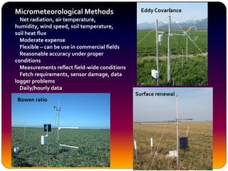
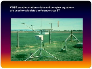
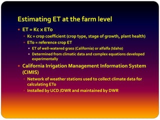
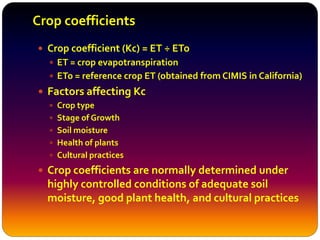
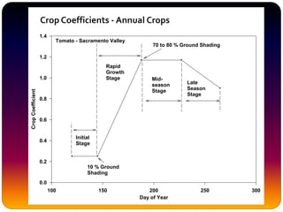
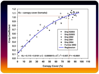
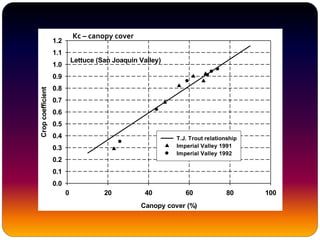
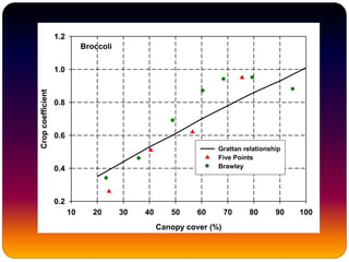
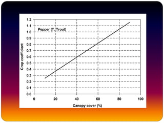
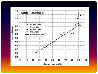
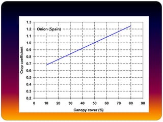
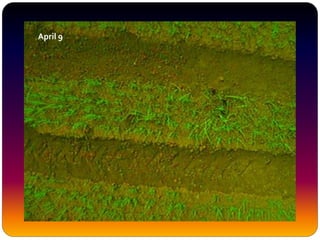
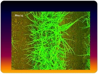
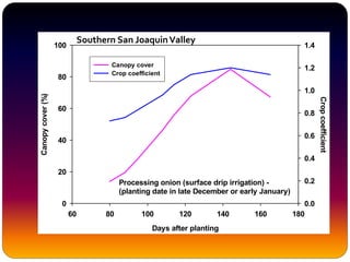
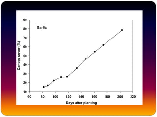
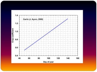
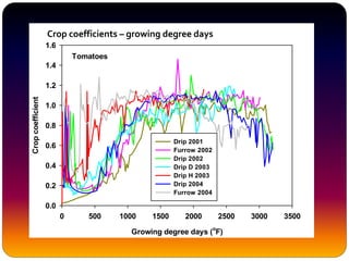
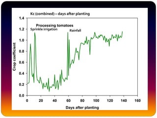
This document discusses crop coefficients, which are used to estimate crop evapotranspiration (ET) from reference evapotranspiration (ETo). It provides the following key points: - Crop coefficients (Kc) account for differences between a crop's ET and a reference crop's ET. Kc values vary by crop type, growth stage, and other factors. - Kc values can be expressed based on calendar day, days after planting, canopy cover percentage, or growing degree days. Expressing Kc as a function of canopy cover may provide more universal relationships. 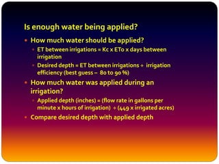- Proper estimation of a crop's Kc allows irrigation managers to determine the desired irrigation amount needed between irrigations based on

1. Crop Coefficients
Blaine Hanson
Department of Land, Air and Water Resources
University of California, Davis

2. Irrigation Water Management:
Science, Art, or Guess?
Blaine Hanson
University of California, Davis

3.  Evapotranspiration = crop water use
 Transpiration (T) - water evaporation from leaves
 Evaporation (E) - water evaporation from soil
 Small plant canopy – E greater thanT
 Large plant canopy -T greater than E
 Most of the evaporation occurs during stand
establishment
 More than 95% of the soil water uptake by plants
becomes transpiration
 Very difficult to separateT and E
 Very difficult to measure ET
Evapotranspiration (ET)

4. Units of evapotranspiration
 Depth of water = volume of water ÷ area
 1 inch of water = amount of water ponded one inch
deep over 1 acre
 1 foot of water = amount of water ponded one foot
deep over 1 acre
 Standardizes water
 Independent of field size
 Crop water use expressed in inches of water is the
same for all fields
 Volume of water (acre-inches) = inches of water x
acres irrigated

5. Crop Evapotranspiration (ET)
MaximumYield
Main cause of ET less than maximum ET
is insufficient soil moisture
Why is ET important?

6. Processing Onion (clay loam)
Applied water (inches)
0 2 4 6 8 10 12 14 16 18 20
Yield(tons/acre)
0
5
10
15
20
25
30
Yield = 0.956 x AW + 6.39; r
2
= 0.99
Note: applied water = ET

7. Measuring evapotranspiration (ET)
 Difficult and expensive to measure
 Even more difficult to separate transpiration and soil
evaporation
 Methods
 Lysimeter
 Meteorological methods
 Soil moisture measurements
 Other

8. Lysimeter
Very expensive
Not practical for commercial
field measurements
Soil/crop characteristics inside
lysimeter similar to those
in immediate vicinity
Potential for accurate
measurements
Daily/hourly values

9. Micrometeorological Methods
Net radiation, air temperature,
humidity, wind speed, soil temperature,
soil heat flux
Moderate expense
Flexible – can be use in commercial fields
Reasonable accuracy under proper
conditions
Measurements reflect field-wide conditions
Fetch requirements, sensor damage, data
logger problems
Daily/hourly data
Eddy Covariance
Bowen ratio
Surface renewal

10. Soil moisture measurements
Relatively inexpensive
Flexible – can be used in
commercial fields
Suitable method – accurate if properly
calibrated, volume of soil measured,
measurement location relative
to root distribution, etc.
Assumes change in soil
moisture over time equals ET (may
not be appropriate under shallow
ground water conditions)
Missing data due to inaccessibility
during and just after irrigation
Daily/hourly values not practical

11. Subsurface drip irrigation (processing tomato)
Days after planting
0 20 40 60 80 100 120 140 160
Dailyevapotranspiration(inchesperday)
0.0
0.1
0.2
0.3
0.4
Evapotranspirattion (ET)
Reference ET (ETo)

12. Subsurface drip irrigation (processing tomato)
Days after planting
0 20 40 60 80 100 120 140 160
YData
0.0
0.1
0.2
0.3
0.4
0.5
ET
E
T
ETo
Sprinkle irrigation
E = 8%;T= 92%

13. Furrow irrigation (processing tomato)
Days after planting
0 20 40 60 80 100 120 140
YData
0.0
0.1
0.2
0.3
0.4
0.5
ET
E
T
ETo
Sprinkle irrigation
Furrow irrigation
E = 15%;T = 85%

14. Sacramento Valley (CH2) 2006
Day of year
0 50 100 150 200 250 300 350 400
Dailyevapotranspiration(inches/day)
0.00
0.05
0.10
0.15
0.20
0.25
0.30
0.35
0.40
Reference ET
ET
Date
Jun 1
May 1 Jul 1
Aug 1
Sep 1
Apr 1
Mar 1
Oct 1
Nov 1
(Alfalfa)

15. Estimating ET at the farm level
 ET = Kc x ETo
 Kc = crop coefficient (crop type, stage of growth, plant health)
 ETo = reference crop ET
 ET of well-watered grass (California) or alfalfa (Idaho)
 Determined from climatic data and complex equations developed
experimentally
 California Irrigation Management Information System
(CIMIS)
 Network of weather stations used to collect climate data for
calculating ETo
 Installed by UCD /DWR and maintained by DWR

16. Crop coefficients
 Crop coefficient (Kc) = ET ÷ ETo
 ET = crop evapotranspiration
 ETo = reference crop ET (obtained from CIMIS in California)
 Factors affecting Kc
 Crop type
 Stage of Growth
 Soil moisture
 Health of plants
 Cultural practices
 Crop coefficients are normally determined under
highly controlled conditions of adequate soil
moisture, good plant health, and cultural practices

17. CIMIS weather station – data and complex equations
are used to calculate a reference crop ET

18. Day of Year
100 150 200 250 300
CropCoefficient
0.0
0.2
0.4
0.6
0.8
1.0
1.2
1.4
Tomato - Sacramento Valley
Initial
Stage
Rapid
Growth
Stage Mid-
season
Stage
Late
Season
Stage
10 % Ground
Shading
70 to 80 % Ground Shading
Crop Coefficients - Annual Crops

19. Types of crop coefficients
 Basil crop coefficients (Kcb)
 Dry soil surface conditions
 Transpiration only
 Dual crop coefficients
 Separate coefficients for evaporation (Kce) and transpiration
(Kcb) conditions
 Kc = Kce + Kcb
 Very little data exist on Kce
 Most evaporation occurs during stand establishment
 Not appropriate for farm level water management
 Combined crop coefficients (Kc)
 Evaporation and transpiration are not separated
 Most common type of crop coefficient

20. Processing tomatoes
Days after planting
0 20 40 60 80 100 120 140 160
Cropcoefficient
0.0
0.2
0.4
0.6
0.8
1.0
1.2
1.4
Kc (combined) – days after planting
Sprinkle irrigation Rainfall

21. Subsurface drip irrigation (processing tomato)
Days after planting
0 20 40 60 80 100 120 140 160
Cropcoefficient
0.0
0.2
0.4
0.6
0.8
1.0
1.2
Kce
Kcb

22. Expressing crop coefficients (Kc)
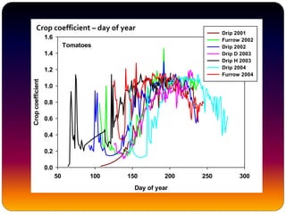
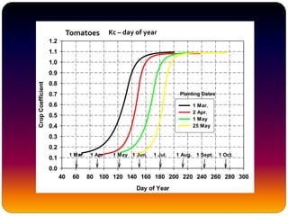
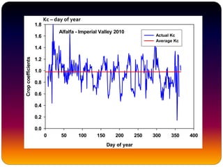
 Kc - calendar (day of year) basis: site, time, and climate
specific
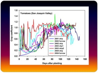
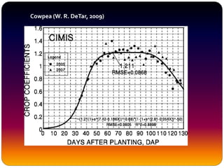
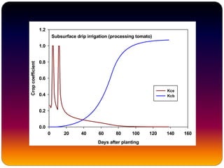
 Kc - days after planting: site, time, and climate specific
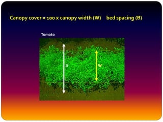
 Kc - canopy cover: universal?, limited data; requires
measuring canopy cover during the crop season
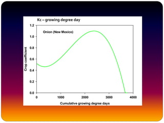
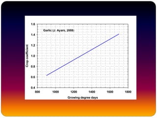
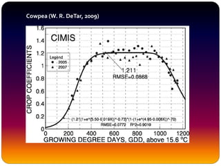
 Kc - growing degree days (heat units): universal?,
calculated values of growing degree days not available
in California
 GDD = [(Tmax –Tmin) ÷ 2] –Tbase
 Tmax = maximum daily temperature
 Tmin = minimum daily temperature
 Tbase = minimum temperature at which no plant growth occurs

23. Kc – day of year or days after planting
relationships

24. Tomatoes
Day of year
50 100 150 200 250 300
Cropcoefficient
0.0
0.2
0.4
0.6
0.8
1.0
1.2
1.4
1.6
Drip 2001
Furrow 2002
Drip 2002
Drip D 2003
Drip H 2003
Drip 2004
Furrow 2004
Crop coefficient – day of year

25. Day of Year
40 60 80 100 120 140 160 180 200 220 240 260 280 300
CropCoefficient
0.0
0.1
0.2
0.3
0.4
0.5
0.6
0.7
0.8
0.9
1.0
1.1
1.2
1 Mar.
2 Apr.
1 May
25 May
1 Mar. 1 Apr. 1 May 1 Jun. 1 Jul. 1 Aug. 1 Sept. 1 Oct.
Planting Dates
Tomatoes Kc – day of year

26. Kc – days after plantingTomatoes (San Joaquin Valley)
Days after planting
0 20 40 60 80 100 120 140 160
Cropcoefficient
0.0
0.2
0.4
0.6
0.8
1.0
1.2
1.4
1.6
2001 drip
2002 furrow
2002 drip
2003 drp1
2003 drip2
2004 drip
2004 furrow

27. Alfalfa - Imperial Valley 2010
Day of year
0 50 100 150 200 250 300 350 400
Cropcoefficients
0.0
0.2
0.4
0.6
0.8
1.0
1.2
1.4
1.6
1.8
Actual Kc
Average Kc
Kc – day of year

28. Cowpea (W. R. DeTar, 2009)

29. Kc – canopy cover (C) relationships
Canopy cover = percent of soil surface shaded by the plant
cover at mid-day

30. Canopy cover = 100 x canopy width (W) bed spacing (B)
B
Tomato

31. Canopy Cover (%)
0 10 20 30 40 50 60 70 80 90 100 110
CropCoefficient
0.0
0.1
0.2
0.3
0.4
0.5
0.6
0.7
0.8
0.9
1.0
1.1
1.2
Drip H2003
Drip D2003
Drip 2002
Drip 2001
Drip 2004
Furrow 2002
Regression
Kc = 0.115 + 0.0181 x C - 0.0000815 x C2
; r2
= 0.957; P = <0.0001
Kc – canopy cover (tomato)

32. Lettuce (San Joaquin Valley)
Canopy cover (%)
0 20 40 60 80 100
Cropcoefficient
0.0
0.1
0.2
0.3
0.4
0.5
0.6
0.7
0.8
0.9
1.0
1.1
1.2
T.J. Trout relationship
Imperial Valley 1991
Imperial Valley 1992
Kc – canopy cover

33. Broccoli
Canopy cover (%)
10 20 30 40 50 60 70 80 90 100
Cropcoefficient
0.2
0.4
0.6
0.8
1.0
1.2
Grattan relationship
Five Points
Brawley

34. Pepper (T. Trout)
Canopy cover (%)
0 20 40 60 80 100
Cropcoefficient
0.0
0.1
0.2
0.3
0.4
0.5
0.6
0.7
0.8
0.9
1.0
1.1
1.2

35. Cotton (R. Hutmacher)
Canopy cover (%)
0 10 20 30 40 50 60 70 80 90 100
Cropcoefficient
0.1
0.2
0.3
0.4
0.5
0.6
0.7
0.8
0.9
1.0
1.1
1.2
1.3
GC510 1992
Pima 1992
GC510 1993
Pima 1993
Regression line

36. Canopy cover (%)
0 10 20 30 40 50 60 70 80 90
Cropcoefficient
0.2
0.3
0.4
0.5
0.6
0.7
0.8
0.9
1.0
1.1
1.2
1.3
Onion (Spain)

37. April 9

38. May 15

39. Processing onion (surface drip irrigation) -
(planting date in late December or early January)
Days after planting
60 80 100 120 140 160 180
Canopycover(%)
0
20
40
60
80
100
Cropcoefficient
0.0
0.2
0.4
0.6
0.8
1.0
1.2
1.4
Canopy cover
Crop coefficient
Southern San JoaquinValley

40. Garlic
Days after planting
60 80 100 120 140 160 180 200 220
Canopycover(%)
10
20
30
40
50
60
70
80
90

41. Garlic (February 25)

42. Garlic (J. Ayars, 2008)
Day of year
40 60 80 100 120 140 160
Cropcoefficient
0.4
0.6
0.8
1.0
1.2
1.4

43. Kc – growing degree days relationships

44. Onion (New Mexico)
Cumulative growing degree days
0 1000 2000 3000 4000
Cropcoefficient
0.0
0.2
0.4
0.6
0.8
1.0
1.2
Kc – growing degree day

45. Garlic (J. Ayars, 2008)
Growing degree days
800 1000 1200 1400 1600 1800
Cropcoefficient
0.4
0.6
0.8
1.0
1.2
1.4
1.6

46. Cowpea (W. R. DeTar, 2009)

47. Tomatoes
Growing degree days (o
F)
0 500 1000 1500 2000 2500 3000 3500
Cropcoefficient
0.0
0.2
0.4
0.6
0.8
1.0
1.2
1.4
1.6
Drip 2001
Furrow 2002
Drip 2002
Drip D 2003
Drip H 2003
Drip 2004
Furrow 2004
Crop coefficients – growing degree days

48. Is enough water being applied?
 How much water should be applied?
 ET between irrigations = Kc x ETo x days between
irrigation
 Desired depth = ET between irrigations ÷ irrigation
efficiency (best guess – 80 to 90 %)
 How much water was applied during an
irrigation?
 Applied depth (inches) = (flow rate in gallons per
minute x hours of irrigation) ÷ (449 x irrigated acres)
 Compare desired depth with applied depth

49. Concerns
 The science part of irrigation water management
 ET and ETo data, crop coefficients
 Site and time specific
 Limited number of experiments
 Kc – canopy cover relationships appear to be more universal
than other crop coefficient relationships
 Problems
 Effect of field to field variability on ET and Kc – climate , soil,
cultural practices
 Effect of year to year variability on ET and Kc – year to year
climate changes, cultural practices
 The art and guess of irrigation water management
 Trying to make limited scientific data developed under a
particular time/site-specific situation fit a particular farm

50. Recommendation
 Use ETo and crop coefficients to
determine how much water should be
applied
 Use flow meters to determine if enough
water was applied
 Monitor soil moisture status with
Watermark sensors
 Determine adequacy of irrigation
 Wetting patterns

51. Onion - four inches from drip line
120 140 160 180 200 220
Soilmoisturetension(centibars)
0
20
40
60
80
100
120
140
160
180
200
6
12
18
24
Onion - 10 inches from drip line
Day of year
120 140 160 180 200 220
0
20
40
60
80
100
120
140
160
180
200
6
12
18
24
Depth (inches)
Depth (inches)
May 1 June 1 July 1 August 1

52. Life is Good