A Markov model assumes that the current state captures all relevant information for predicting the future. It can be used for language modeling by assigning probabilities to word sequences. Google's PageRank algorithm ranks web pages based on the principle that more authoritative pages, as determined by other pages linking to them, should rank higher. It models the probability of being on a page as a stationary distribution of a Markov chain defined by the link structure of the web.
Kernel functions allow measuring the similarity between objects without explicitly representing them as feature vectors. The kernel trick enables applying algorithms designed for explicit feature vectors, like support vector machines (SVMs), to implicit spaces defined by kernels. SVMs find a sparse set of support vectors that define the decision boundary by maximizing margin and minimizing error. They can perform both classification using a hinge loss function and regression using an epsilon-insensitive loss function.
This document discusses sparse linear models and Bayesian variable selection. It introduces the spike and slab model for Bayesian variable selection, which uses a binary vector γ to indicate whether features are relevant or not. Computing the posterior p(γ|D) involves calculating the marginal likelihood p(D|γ). Greedy search and stochastic search methods are discussed to approximate the posterior over models. L1 regularization, also known as lasso, is introduced as an optimization technique since computing the posterior for discrete γ is difficult. Lasso replaces the discrete priors with continuous priors to encourage sparsity. Coordinate descent is discussed as an algorithm to optimize the lasso objective function.
This document describes a simulation of kidney tumor growth to determine the probability that a tumor formed before a patient's retirement from the military. The simulation models tumor growth rates based on data from a medical study. It generates random growth rates from a fitted distribution and simulates tumor size over time. The results are cached in a joint distribution of size and age. Conditional distributions of age given size are extracted and percentiles plotted to summarize the results. Potential issues with the modeling assumptions are discussed, including the effects of non-spherical tumor shapes and serial correlation in growth rates over time.
This document describes using Bayesian inference to locate an opponent in a two-dimensional paintball arena based on the locations of paint spatters on the wall. It defines a joint distribution over all possible (x,y) coordinates of the opponent's location. Given observed spatter locations, it computes the posterior distribution, which provides the likelihood of each possible location. This allows extracting marginal and conditional distributions over each dimension, as well as computing credible intervals to identify likely regions where the opponent may be hiding.
EM 알고리즘을 jensen's inequality부터 천천히 잘 설명되어있다
이것을 보면, LDA의 Variational method로 학습하는 방식이 어느정도 이해가 갈 것이다.
옛날 Andrew Ng 선생님의 강의노트에서 발췌한 건데 5년전에 본 것을
아직도 찾아가면서 참고하면서 해야 된다는 게 그 강의가 얼마나 명강의였는지 새삼 느끼게 된다.
This document describes using a feature-based Markov Decision Process (MDP) and policy iteration to develop an algorithm that learns to play the game Tetris well. It formulates Tetris as an MDP with states defined by wall configurations and piece placement. An approximated value function is defined using features of the game state like column heights. Policy iteration is then used to iteratively update the weight vector of this approximated value function to learn an optimal policy. Simulation results show the learning algorithm achieves much higher scores on Tetris compared to a heuristic algorithm.
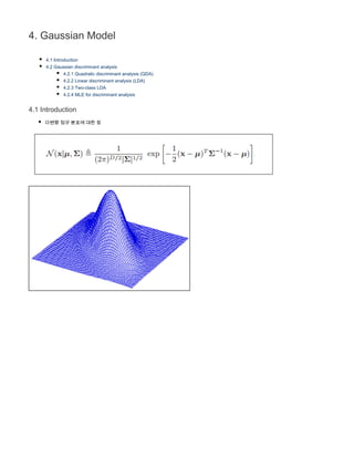
1. 4. Gaussian Model
4.1 Introduction
4.2 Gaussian discriminant analysis
4.2.1 Quadratic discriminant analysis (QDA)
4.2.2 Linear discriminant analysis (LDA)
4.2.3 Two-class LDA
4.2.4 MLE for discriminant analysis
4.1 Introduction
다변량 정규 분포에 대한 장
2.
3. 4.2 Gaussian discriminant analysis
Class가 주어졌을 때, feature vector는 Gaussian 분포라는 가정이 주어진다
(Gaussian) discriminant analysis: posterior
(2.13) //p(x|y)는 정규분포
예를 들어 2-class 문제의 경우
판별하는데 필요한 μc,Σc 는 MLE 추정으로 구한다(섹션 4.2.4), 즉 각 클래스마다 샘플 평균, 샘플 공분산
예를 들어 2-class의 경우, 데이터의 likelihood는
4. 파라메터 추정치는
Decision Rule: class 분류에 상관없는 분모는 지우고 log를 취해서 가장 큰 posterior를 갖는 class로 분류
모든 class가 균일한 prior 분포를 가졌다면, 위의 수식에서 첫번째 prior항은 없어지고 두번째 항에 정규 분포 수식을 대입
4.2.1 Quadratic discriminant analysis (QDA)
식 (2.13)에 likelihood와 prior에 각각 multinomial 분포식과 정규 분포식을 대입하면
(4.33)
위의 식을 class를 결정하는 x에 대한 함수로 본다면(p(y=1|x) - p(y=0|x) > 0 이면 y=1과 같은) 이차식(quadratic)의 형태이고 분류
평면(p(y=1|x) = p(y=0|x)인 지점)도 다음과 같이 곡선이 나오게 된다
5. 4.2.2 Linear discriminant analysis (LDA)
모든 class에 대해서 공분산을 공유한다면(또는 같다면)
즉
이라면
(4.33)은 다음과 같이 된다.
이차 항 xT
Σ-1
x은 모든 class에 대해서 동일하므로 분류에 영향을 끼치지 않기 때문에 사라지고, decision boundary는 linear해 진다.
라고 두면 식(4.35)는 다음과 같이 쓸 수 있고
(4.38)
이러한 모양의 함수는 soft한 max함수처럼 작용하기 때문에 S는 softmax 함수라고 불린다.
예를 들어 η = (3,0,1)이라면 다음과 같이 최대값인 3에 대해서 0.8정도의 확률이 할당된다
6. 4.2.3 Two-class LDA
2-class 문제를 가정하고 식 (4.38)에 log를 취해서 다음과 같이 linear한 평면을 유도할 수 있다.
βc'- βc항이 분류 평면의 법선 벡터가 되고 γc'- γc항이 분류 평면의 bias가 된다.
4.2.4 MLE for discriminant analysis
수식 (4.35)의 mu와 sigma는 다음과 같이 MLE로 추정할 수 있고 결과는 다음과 같다
즉, 각 class에 대해서 feature vector들의 평균과 분산이다.